spectral algorithms for supervised learning - dimadevito/pub_con/spectralneco.pdfspectral algorithms...

LETTER Communicated by David Hardoon

Spectral Algorithms for Supervised Learning

L. Lo [email protected]. [email protected]. [email protected] di Informatica e Scienze dell’Informazione, Universita di Genova,16146 Genoa, Italy

E. De [email protected] di Scienze per l’Architettura, Universita di Genova, and IstitutoNazionale di Fisica Nucleare, Genova, Italy

A. [email protected] di Informatica e Scienze dell’Informazione, Universita di Genova,16146 Genoa, Italy

We discuss how a large class of regularization methods, collectivelyknown as spectral regularization and originally designed for solvingill-posed inverse problems, gives rise to regularized learning algorithms.All of these algorithms are consistent kernel methods that can be easilyimplemented. The intuition behind their derivation is that the sameprinciple allowing for the numerical stabilization of a matrix inversionproblem is crucial to avoid overfitting. The various methods have a com-mon derivation but different computational and theoretical properties.We describe examples of such algorithms, analyze their classificationperformance on several data sets and discuss their applicability toreal-world problems.

1 Introduction

A large amount of literature has pointed out the connection between algo-rithms in learning theory and regularization methods in inverse problems(see, e.g., Vapnik, 1982, 1998; Poggio & Girosi, 1992; Evgeniou, Pontil, &Poggio, 2000; Hastie, Tibshirani, & Friedman, 2001; Scholkopf & Smola,2002; De Vito, Rosasco, Caponnetto, De Giovannini, & Odone, 2005).The main message is that regularization techniques provide stability with

Neural Computation 20, 1873–1897 (2008) C© 2008 Massachusetts Institute of Technology

1874 L. Lo Gerfo et al.

respect to noise and sampling, therefore ensuring good generalization prop-erties to the corresponding learning algorithms. Usually regularization inlearning is based on the minimization of a functional in a suitable hypothesisspace—for example, the penalized empirical error on a reproducing kernelHilbert space. Hence, theoretical analysis focuses mainly on the choice ofthe loss function, the penalty term, and the kernel (Vapnik, 1998; Evgeniouet al., 2000; Scholkopf & Smola, 2002; Hastie et al., 2001).

From the seminal work of Tikhonov and others (Tikhonov & Arsenin,1977), regularization has been rigorously defined in the theory of ill-posed inverse problems. In this context, the problem is to invert alinear operator (or a matrix) that might have an unbounded inverse (ora bad condition number). Regularization amounts to replacing the ori-ginal operator with a bounded operator, namely, the regularization opera-tor (Engl, Hanke, & Neubauer, 1996), whose condition number is controlledby a regularization parameter. The regularization parameter should be cho-sen according to the noise level in order to ensure stability. Many regu-larization algorithms are known; Tikhonov and truncated singular valuedecomposition (TSVD) are probably the most commonly used.

As Bertero and Boccacci (1998) noted, one can also regard regularizationfrom a signal processing perspective introducing the notion of filter. Thispoint of view gives a way of looking constructively at regularization;indeed, each regularization operator can be defined using spectral calculusas a suitable filter on the eigendecomposition of the operator definingthe problem. The filter is designed to suppress the oscillatory behaviorcorresponding to small eigenvalues. In this view, it is known, for example,that Tikhonov regularization can be related to the Wiener filter (Bertero &Boccacci, 1998).

Regularization has a long history in learning, and our starting point isthe theoretical analysis proposed in Bauer, Pereverzev, and Rosasco (2007),De Vito, Rosasco, and Verri (2005), Caponnetto and De Vito (2007), andCaponnetto (2006), showing that many regularization methods originallyproposed in the context of inverse problems give rise to consistent kernelmethods with optimal minimax learning rates. The analysis we propose inthis letter focuses on three points.

First, in contrast to Bauer et al. (2007), we propose a more intuitivederivation of regularization based on the notion of spectral filter. We start byintroducing the notion of filter functions and explain why, besides ensuringnumerical stability, they can also provide a way to learn with generalizationguarantees. This requires, in particular, discussing the interplay betweenfiltering and random sampling. Our analysis is complementary to the theorydeveloped in Bauer et al. (2007), De Vito, Rosasco, and Verri (2005), Yao,Rosasco, and Caponnetto (2007), and Caponnetto (2006). Note that the factthat algorithms ensuring numerical stability can also learn is not obviousbut confirms the deep connection between stability and generalization (for

Spectral Algorithms for Supervised Learning 1875

references, see Bousquet & Elisseeff, 2002; Poggio, Rifkin, Mukherjee, &Niyogi, 2004; Rakhlin, Mukherjee, & Poggio, 2005).

Second, we present and discuss several examples of filters inducingspectral algorithms for supervised learning. The filter function perspec-tive provides a unifying framework for discussing similarities and differ-ences among the various methods. Some of these algorithms, such as theν-method and iterated Tikhonov, are new to learning. Other algorithmsare well known: spectral cut-off (TSVD) is related to principal componentregression (PCR) and its kernel version; Landweber iteration is knownas L2-boosting (Buhlmann & Yu, 2002), and Tikhonov regularization isalso known as regularized least squares or ridge regression. Our analy-sis highlights the common regularization principle underlying algorithmsoriginally motivated by seemingly unrelated ideas: penalized empiricalrisk minimization, like regularized least squares; early stopping of iterativeprocedures, like gradient descent; and (kernel) dimensionality reductionmethods, like (kernel) principal component analysis.

Despite these similarities, spectral algorithms have differences from bothcomputational and theoretical points of view. One of the main differences re-gards the so-called saturation effect affecting some regularization schemes.This phenomenon, which is well known in inverse problem theory, amountsto the impossibility for some algorithms to exploit the regularity of the tar-get function beyond a certain critical value, referred to as the qualificationof the method. We try to shed light on this, which is usually not discussedin the literature of learning rates, using some theoretical considerations andnumerical simulations.

Another point that differentiates spectral algorithms concerns algorith-mic complexity. An interesting aspect is the built-in property of iterativemethods to recover solutions corresponding to the whole regularizationpath (Hastie, Rosset, Tibshirani, & Zhu, 2004).

Third, we evaluate the effectiveness of the proposed algorithms inlearning tasks with an extensive experimental study. The performance ofthese spectral algorithms is assessed on various data sets, and it is com-pared against state-of-the-art techniques, such as support vector machines(SVMs). The above algorithms often improve the state-of-the-art results andhave interesting computational properties, such as the fact that the imple-mentation amounts to a few lines of code. Optimization issues that mightbe interesting starting points for future work are beyond the scope of thisresearch (see the recent work of Li, Lee, & Leung, 2007, for references).

The plan of the letter is the following. Section 2 discusses previous worksin the context of filtering and learning, section 3 reviews the regularizedleast-squares algorithm from a filter function perspective, and section 4is devoted to extending the filter point of view to a large class of ker-nel methods. In section 5 we give several examples of such algorithmsand discuss their properties and complexity in section 6. Section 7 reports


results obtained with an experimental analysis on various data sets, andsection 8 contains a final discussion.

2 Previous Work on Learning, Regularization, and Spectral Filtering

The idea of using regularization in statistics and machine learning haslong been explored (see, e.g., Wahba, 1990; Poggio & Girosi, 1992), and theconnection between large margin kernel methods such as support vectormachines and regularization is well known (see Vapnik, 1998; Evgeniouet al., 2000; Scholkopf & Smola, 2002). Ideas coming from inverse prob-lems mostly used Tikhonov regularization and were extended to severalerror measures other than the quadratic loss function. The gradient descentlearning algorithm in Yao et al. (2007) can be seen as an instance of Landwe-ber iteration (Engl et al., 1996) and is related to the L2 boosting algorithm(Buhlmann & Yu, 2002). For iterative methods, some partial results, whichdo not take into account the random sampling, are presented in Ong andCanu (2004) and Ong, Mary, Canu, and Smola (2004). The interplay of ill-posedness, stability, and generalization is not new to learning (Poggio &Girosi, 1992; Evgeniou et al., 2000; Bousquet & Elisseeff, 2002; Rakhlin et al.,2005; Poggio et al., 2004; De Vito, Rosasco, Caponnetto, et al., 2005).

The notion of filter function was previously studied in machine learningand gives a connection to the literature of function approximation in signalprocessing and approximation theory. The pioneering work of Poggio andGirosi (1992) established the relation between neural networks, radial basisfunctions, and regularization. Though the notion of reproducing kernel isnot explicitly advocated, Green functions of second-order differential oper-ator are used to define penalties for penalized empirical risk minimization.Filtering and reweighing of the Fourier transform of Green functions areused de facto to design new kernels (see also for the relation between kerneland penalty term in Tikhonov regularization). Poggio and Girosi (1992), aswell as Girosi, Jones, and Poggio (1995), are suitable sources for referenceand discussion. An important aspect that we would like to stress is thatfrom a technical point of view, these works implicitly assume the data tobe sampled according to a uniform distribution and make extensive use ofFourier theory. Indeed the extension to general probability distribution isnot straightforward, and this is crucial since it is standard in learning theoryto assume the point to be drawn according to a general, unknown distri-bution. A mathematical connection between sampling theory and learningtheory has been recently proposed by Smale and Zhou (2004, 2005) whereasDe Vito, Rosasco, Caponnetto, et al. (2005) and De Vito et al. (2006) gavean inverse problem perspective on learning. The analysis we present canbe seen as a further step toward a deeper understanding of learning as afunction approximation problem.

Recently filtering of the kernel matrix has been considered in the con-text of graph regularization (see Hastie et al., 2001; Chapelle, Weston, &


Scholkopf, 2003; Zhu, Kandola, Ghahramani, & Lafferty, 2005; Smola &Kondor, 2003; Zhang & Ando, 2006). In this case, reweighing of a kernelmatrix (filters) on a set of labeled and unlabeled input points is used todefine new penalty terms, replacing the square of the norm in the adoptedhypothesis space. It has been shown (see, e.g., Zhang & Ando, 2006) thatthis is equivalent to standard regularized least squares with data-dependentkernels. Note that in graph regularization, no sampling is considered, andthe problem is truly a problem of transductive learning.

Our analysis relies on a different use of filter functions to define newalgorithms rather the new kernels. In fact, in our setting, the kernel isfixed, and each rescaling of the kernel matrix leads to a learning algorithm,which is not necessarily a penalized minimization. The dependence of therescaling on the regularization parameter allows us to derive consistencyresults in a natural way.

3 Regularized Least Squares as a Spectral Filter

In this section we review how the generalization property of the regular-ized least-squares algorithm is a consequence of the algorithm being seenas a filter on the eigenvalues of the kernel matrix. This point of view natu-rally suggests a new class of learning algorithms defined in terms of filterfunctions, whose properties are discussed in the next section.

In the framework of supervised learning, the regularized least-squaresalgorithm is based on the choice of a Mercer kernel1 K (x, t) on the inputspace X and a regularization parameter λ > 0. Hence, for each trainingset z = (x, y) = {(x1, y1), . . . , (xn, yn)} of n-examples (xi , yi ) ∈ X × R, regu-larized least squares amounts to

f λz (x) =

n∑i=1

αi K (x, xi ) with α = (K + nλI )−1y, (3.1)

where K is the n × n-matrix (K)i j = K (xi , xj ).Since λ > 0, it is clear that we are numerically stabilizing a matrix in-

version problem that is possibly ill conditioned (i.e., numerically unstable).Before showing that regularized least squares can be seen as a suitable fil-tering of the kernel matrix, able to ensure good generalization properties ofthe estimator, we first need to recall some basic concepts of learning theory.

We assume that the examples (xi , yi ) are drawn identically and in-dependently distributed according to an unknown probability measureρ(x, y) = ρ(y | x)ρX(x). Moreover, we assume that X is a compact subset ofR

d , and the labels yi belong to a bounded subset Y ⊂ R (e.g., in a binaryclassification problem Y = {−1, 1}). Finally, we assume that the kernel K

1This means that K : X × X → R is a symmetric continuous function, which is positivedefinite (Aronszajn, 1950).


is bounded by 1 and is universal (see Micchelli, Xu, & Zhang, 2006, andreferences therein), that is, the set of functions

H ={

N∑i=1

αi K (x, xi ) | xi ∈ X, αi ∈ R

}

is dense in L2(X), the Hilbert space of functions that are square-integrablewith respect to ρX.

With the choice of the square loss, the generalization property of the esti-mator means that the estimator f λ

z is a good approximation of the regressionfunction,

fρ(x) =∫

Yy dρ(y | x),

with respect to the norm of L2(X). In particular, the algorithm is (weakly)consistent (Vapnik, 1998) if, for a suitable choice of the parameter λ = λn asa function of the examples,

limn→∞

∫X

(f λz (x) − fρ(x)

)2dρX(x) = lim

n→∞∥∥ f λ

z − fρ∥∥2

ρ= 0,

with high probability (see, e.g., Vapnik, 1998).Notice that in classification, the goal is to approximate the Bayes rule sign

( fρ) = sign(ρ(1 | x) − 1/2) with the plug-in estimator sign( f λz ) with respect

to the classification error R( f λz ) = P(yf λ

z (x) < 0). In any case the followingbound holds,

R(

f λz

) − R( fρ) ≤ ∥∥ f λz − fρ

∥∥ρ

(3.2)

(see, e.g., Bartlett, Jordan, & McAuliffe, 2006), so in the following discussionwe consider only the square loss.

We start by rewriting equation 3.1 in a slightly different way:

(f λz (x1), . . . , f λ

z (xn)) = K

n

(Kn

+ λ

)−1

y. (3.3)

Observe that if v is an eigenvector of K/n with eigenvalue σ , then we haveKn ( K

n + λ)−1v = σσ+λ

v, so that the regularized least-squares algorithm is infact a filter on the eigenvalues of the kernel matrix.

The filter σσ+λ

ensures not only numerical stability but also the gen-eralization properties of the estimator. To obtain insight into this point,consider the population case when we have knowledge of the probability


distribution ρ generating the data. In this setting, the kernel matrix K/n isreplaced by the integral operator L K with kernel K ,

L K f (x) =∫

XK (x, s) f (s)dρX(s) f ∈ L2(X), (3.4)

and the data y is replaced by the regression function fρ , so that equation 3.3becomes

f λ = L K (L K + λI )−1 fρ. (3.5)

More explicitly, since L K is a positive compact operator bounded by 1 andH is dense in L2(X), there is basis (ui )i≥1 in L2(X) such that L K ui = σi ui

with 0 < σi ≤ 1 and limi→∞ σi = 0. Hence,

fρ =∞∑

i=1

〈 fρ, ui 〉ρui

f λ =∞∑

i=1

σi

σi + λ〈 fρ, ui 〉ρui .

A comparison of the two equations shows that f λ is a good approximationof fρ provided that λ is small enough. For such λ, the filter σ

σ+λselects only

the components of the fρ corresponding to large eigenvalues, which are afinite number since the sequence of eigenvalues goes to zero. Hence, if weslightly perturb both L K and fρ , the corresponding solution of equation 3.4is close to fρ provided that the perturbation is small. The key idea is thatnow we can regard the sample case K, y and the corresponding estima-tor f λ

z , as a perturbation of L K , fρ , and f λ, respectively. A mathematicalproof of the above intuition requires some work, and we refer to De Vito,Rosasco, and Verri (2005) and Bauer et al. (2007) for the technical details.The basic idea is that the law of large numbers ensures that the perturbationis small, provided that the number of examples is large enough and, as aconsequence, f λ

z is close to f λ and hence to fρ .The discussion suggests that one can replace σ

σ+λwith other functions

σgλ(σ ) that are filters on the eigenvalues of L K and obtain different regu-larization algorithms, as shown in the next section.

4 Kernel Methods from Spectral Filtering

In this section we discuss the properties of kernel methods based on spec-tral filtering. Our approach is inspired by inverse problems. A completetheoretical discussion of our approach can be found in De Vito, Rosasco,and Verri (2005), Bauer et al. (2007), and Caponnetto (2006).


Let K be a Mercer kernel as in the above section. Looking at equation 3.1suggests defining a new class of learning algorithm by letting

f λz (x) =

n∑i=1

αi K (x, xi ) with α = 1n

gλ

(Kn

)y, (4.1)

where gλ: [0, 1] → R is a suitable function and gλ( Kn ) is defined by spectral

calculus; that is, if v is an eigenvector of K/n with eigenvalue σ (sinceK is a Mercer kernel bounded by 1, 0 ≤ σ ≤ 1), then gλ( K

n )v = gλ(σ )v. Inparticular, on the given data, one has

(f λz (x1), . . . , f λ

z (xn)) = K

ngλ

(Kn

)y. (4.2)

We note that unlike regularized least squares, such an estimator is notnecessarily the solution of penalized empirical minimization. Clearly, toensure both numerical stability and consistency, we need to make someassumptions on gλ. Following De Vito, Rosasco, and Verri (2005) and Baueret al. (2007), we say that a function gλ : [0, 1] → R parameterized by 0 <

λ ≤ 1 is an admissible filter function if:

1. There exists a constant B such that

sup0<σ≤1

|gλ(σ )| ≤ Bλ

∀λ ∈ [0, 1]. (4.3)

2. There exists a constant D such that

limλ→0

σgλ(σ ) = 1 ∀σ ∈ ]0, 1]

sup0<σ≤1

|σgλ(σ )| ≤ D ∀λ ∈ [0, 1]. (4.4)

3. There is a constant ν > 0, namely, the qualification of the regulariza-tion gλ, such that

sup0<σ≤1

|1 − gλ(σ )σ |σ ν ≤ γνλν, ∀ 0 < ν ≤ ν, (4.5)

where the constant γν > 0 does not depend on λ.

A simple computation shows that gλ(σ ) = 1σ+λ

is an admissible filterfunction; indeed equations 4.3 and 4.4 hold with B = D = 1, condition 4.5is verified with γν = 1 for 0 < ν ≤ 1, and hence the qualification equals 1.Other examples are discussed in the next section. Here we give a heuristicmotivation of the above conditions, keeping in mind the discussion in the


previous section. First, observe that the population version of equation 4.1becomes

f λ =∑

i

σi gλ(σi )〈 fρ, ui 〉ρui . (4.6)

We can make the following observations.

1) Equation 4.3 ensures that eigenvalues of gλ(K) are bounded by Bλ

, sothat equation 4.1 is numerically stable. Moreover, looking at equa-tion 4.6, we see that it also implies that if σi is much smaller than λ,the corresponding Fourier coefficient 〈 f λui 〉 of f λ is small. Hence, f λ

has essentially only a finite number of nonzero Fourier coefficients onthe basis (ui )i≥1, and we can argue that by the law of large numbers,f λz is a good approximation of f λ when n is large enough.

2) Assumption 4.4 implies that f λ converges to fρ if λ goes to zero. Interms of the kernel matrix, this condition means that gλ(K) convergesto K−1 when λ goes to zero, avoiding oversmoothing.

3) Condition 4.5 is related to the convergence rates of the algorithm.These rates depend on how fast the Fourier coefficients 〈 fρ, ui 〉 con-verge to 0 with respect to the eigenvalues σi (Bauer et al., 2007). Thisinformation is encoded by a priori assumptions on fρ of the form

∞∑i=1

〈 fρ, ui 〉2ρ

σ 2ri

< R, (4.7)

where the parameter r encodes the regularity property of the regres-sion function. If r = 1/2, this corresponds to assuming fρ ∈ H and,more generally, the larger is r , the smoother is the function. Condi-tion 4.5 and the choice λn = 1

n2r+1 ensure that if r ≤ ν,∥∥ f λnz − fρ

∥∥ρ

≤ Cn− r2r+1 with high probability, (4.8)

whereas if r ≥ ν, the rate of convergence is always n− ν2ν+1 (for proof

and a complete discussion, see Bauer et al., 2007; Caponnetto, 2006).Hence, filter functions having a larger qualification ν give better rates,that is, the corresponding algorithms can better exploit the smooth-ness of fρ . This fact marks a big distinction among the various algo-rithms we consider, as we discuss in the following. Also, notice thatin the classification setting we will consider in our experiments, ifr ≤ ν bounds 3.2 and equation 4.8 give that

R(

f λz

) − inffR( f ) = O

(n− r

2r+1)

with high probability.


Considering the decomposition f λz − fρ = ( f λ

z − f λ) + ( f λ − fρ), fromthe above discussion, we have that the consistency of this class of learn-ing algorithms depends on two opposite terms: the approximation error‖ f λ − fρ‖ and the sample error ‖ f λ

z − f λ‖. The approximation error de-pends on the examples only through λ = λn, and it decreases if λ goes tozero, whereas the sample error is of a probabilistic nature and it increases ifλ goes to zero. The optimal choice of the regularization parameter λ will bea trade-off between these two errors (see De Vito, Caponnetto, & Rosasco,2005; Caponnetto & De Vito, 2006; Smale & Zhou, 2007; Wu, Ying, & Zhou,2006), about the rates for regularized least-squares. See De Vito, Rosasco,and Verri (2005), Bauer et al. (2007), and Caponnetto (2006), for arbitraryfilters.

Before giving several examples of algorithms that fit into the above gen-eral framework, we observe that the considered algorithms can be regardedas filters on the expansion of the target function on a suitable basis. In prin-ciple, this basis can be obtained from the spectral decomposition of theintegral operator L K and in practice is approximated by considering thespectral decomposition of the kernel matrix K. Interestingly, the basis thusobtained has a natural interpretation: if the data are centered (in the featurespace), then the elements of the basis are the principal components of theexpected (and empirical) covariance matrix in the feature space. In this re-spect, the spectral methods we discussed rely on the assumption that mostof the information is actually encoded in the first principal components.

5 The Proposed Algorithms

In this section we give specific examples of kernel methods based on spec-tral regularization. All of these algorithms are known in the context ofregularization for linear inverse problems, but only some of them havebeen used for statistical inference problems. These methods have many in-teresting features: from the algorithmic point of view, they are simple toimplement; usually they amount to a few lines of code. They are appealingfor applications: their model selection is simple since they depend on fewparameters, and overfitting may be dealt with in a very transparent way.Some of them represent a very good alternative to regularized least squares(RLS) because they are faster without compromising classification perfor-mance (see section 7). Note that for regularized least squares, the algorithmhas the following variational formulation,

minf ∈H

1n

n∑i=1

(yi − f (xi ))2 + λ ‖ f ‖2H ,

which can be interpreted as an extension of empirical risk minimiza-tion. In general, the class of regularization might not be described by a


variational problem so that the filter point of view provides us with a suit-able description.

More details on the derivation of these algorithms can be found in Englet al. (1996).

5.1 Iterative Landweber. Landweber iteration is characterized by thefilter function

gt(σ ) = τ

t−1∑i=0

(1 − τσ )i ,

where we identify λ = t−1, t ∈ N and take τ = 1 (since the kernel is boundedby 1). In this case, we have B = D = 1, and the qualification is infinite sinceequation 4.5 holds with γν = 1 if 0 < ν ≤ 1 and γν = νν otherwise. The abovefilter can be derived from a variational point of view. In fact, as shown inYao et al. (2007), this method corresponds to empirical risk minimizationvia gradient descent. If we denote with ‖·‖ n the norm in R

n, we can impose

∇‖Kα − y‖2n = 0,

and by a simple calculation, we see that the solution can be rewritten as thefollowing iterative map,

αi = αi−1 + τ

n(y − Kαi−1), i = 1, . . . , t,

where τ determines the step size. We may start from a very simple solution:α0 = 0. Clearly, if we let the number of iterations grow, we are simplyminimizing the empirical risk and are bound to overfit. Early stopping of theiterative procedure allows us to avoid overfitting; thus, the iteration numberplays the role of the regularization parameter. In Yao et al. (2007), the fixedstep size τ = 1 was shown to be the best choice among the variable stepsize τ = 1

(t+1)θ , with θ ∈ [0, 1). This suggests that τ does not play any role inregularization. Landweber regularization was introduced under the nameof L2-boosting for splines in a fixed design statistical model (Buhlmann &Yu, 2002) and eventually generalized to general RKH spaces and randomdesign in Yao et al. (2007).

5.2 Semi-Iterative Regularization. An interesting class of algorithmsconsists of the so-called semi-iterative regularization or acceleratedLandweber iteration. These methods can be seen as a generalization ofLandweber iteration where the regularization is now

gt(σ ) = pt(σ ),


with pt a polynomial of degree t − 1. In this case, we can identify λ = t−2, t ∈N. One can show that D = 1, B = 2, and the qualification of this class ofmethods is usually finite (Engl et al., 1996).

An example that turns out to be particularly interesting is the so-calledν method. The derivation of this method is fairly complicated and relies onthe use of orthogonal polynomials to obtain acceleration of the standardgradient descent algorithm (see Chapter 10 in Golub & Van Loan, 1996).Such a derivation is beyond the scope of this presentation and we referinterested readers to Engl et al. (1996). In the ν method, the qualification isν (fixed) with γν = c for some positive constant c. The algorithm amountsto solving (with α0 = 0) the following map,

αi = αi−1 + ui (αi−1 − αi−2) + ωi

n(y − Kαi−1), i = 1, . . . , t,

where

ui = (i − 1)(2i − 3)(2i + 2ν − 1)(i + 2ν − 1)(2i + 4ν − 1)(2i + 2ν − 3)

ωi = 4(2i + 2ν − 1)(i + ν − 1)(i + 2ν − 1)(2i + 4ν − 1)

t > 1.

The interest of this method lies in the fact that since the regularizationparameter here is λ = t−2, we just need the square root of the number ofiterations needed by Landweber iteration. In inverse problems, this methodis known to be extremely fast and is often used as a valid alternative to con-jugate gradient (see Engl et al., 1996, Chap. 6, for details). To our knowledge,semi-iterative regularization has not been previously used in learning.

5.3 Spectral Cut-Off. This method, also known as truncated singularvalues decomposition (TSVD), is equivalent to the so-called (kernel) prin-cipal component regression. The filter function is simply

gλ(σ ) ={

1σ

σ ≥ λ

0 σ < λ.

In this case, B = D = 1. The qualification of the method is arbitrary, andγν = 1 for any ν > 0. The corresponding algorithm is based on the followingsimple idea. Perform SVD of the kernel matrix K = USUT , where U is anorthogonal matrix and S = diag(σ1, . . . , σn) is diagonal with σi ≥ σi+1. Then


discard the singular values smaller than the threshold λ, and replace themwith 0. The algorithm is then given by

α = K−1λ y, (5.1)

where K−1λ = UT S−1

λ U and S−1λ = diag(1/σ1, . . . , 1/σm, 0, . . .) where σm ≥ λ

and σm+1 < λ. The regularization parameter is the threshold λ or, equiva-lently, the number m of components that we keep.

Finally, notice that if the data are centered in the feature space, thenthe columns of the matrix U are the principal components of the covariancematrix in the feature space, and the spectral cut-off is a filter that discards theprojection on the last principal components. The procedure is well knownin literature as kernel principal component analysis (see, e.g., Scholkopf &Smola, 2002).

5.4 Iterated Tikhonov. We conclude this section by mentioning amethod that is a mixture between Landweber iteration and Tikhonov reg-ularization. Unlike Tikhonov regularization, which has finite qualificationand cannot exploit the regularity of the solution beyond a certain regularitylevel, iterated Tikhonov overcomes this problem by means of the followingregularization:

gλ(σ ) = (σ + λ)ν − λν

σ (σ + λ)ν, ν ∈ N.

In this case, we have D = 1 and B = t, and the qualification of the methodis now ν with γν = 1 for all 0 < ν ≤ t. The algorithm is described by thefollowing iterative map,

(K + nλI )αi = y + nλαi−1 i = 1, . . . , ν,

choosing α0 = 0. It is easy to see that for ν = 1, we simply recover thestandard Tikhonov regularization, but as we let ν > 1, we improve thequalification of the method with respect to standard Tikhonov. Moreover,we note that by fixing λ, we can think of the above algorithms as an iterativeregularization with ν as the regularization parameter.

6 Different Properties of Spectral Algorithms

In this section, we discuss the differences of the proposed algorithms fromtheoretical and computational viewpoints.

6.1 Qualification and Saturation Effects in Learning. As we mentionedin section 4, one of the main differences among the various spectral methods


Figure 1: The behaviors of the residuals for Tikhonov regularization (left) andTSVD (right) as a function of σ for different values of r and fixed λ.

is their qualification. Each spectral regularization algorithm has a criticalvalue (the qualification) beyond which learning rates no longer improvedespite the regularity of the target function fρ . If this is the case, we saythat methods saturate. In this section, we recall the origin of this problemand illustrate it with some numerical simulations.

Saturation effects have their origin in analytical and geometrical prop-erties rather than in statistical properties of the methods. To see this, recallthe error decomposition f λ

z − fρ = ( f λz − f λ) + ( f λ − fρ), where the latter

term is the approximation error that, recalling equation 4.6, is related to thebehavior of

fρ − f λ =∑

i

〈 fρ, ui 〉ρui −∑

i

σi gλ(σi )〈 fρ, ui 〉ρui

=∑

i

(1 − σi gλ(σi ))σ ri〈 fρ, ui 〉ρ

σ ri

ui . (6.1)

If the regression function satisfies equation 4.7, we have

‖ fρ − f λ‖ρ ≤ R sup0<σ≤1

(|1 − gλ(σ )σ |σ r ).

The above formula clearly motivates condition 4.5 and the definition of qual-ification. In fact, it follows that if r ≤ ν, then ‖ fρ − f λ‖ρ = O(λr ), whereas ifr > ν, we have ‖ fρ − f λ‖ρ = O(λν). To avoid confusion, note that the indexr in the equation 6.1 encodes a regularity property of the target function,whereas ν in equation 4.5 encodes a property of the given algorithm.

In Figure 1, we show the behaviors of the residual (1 − σgλ(σ ))σ r

as a function of σ for different values of r and fixed λ. For Tikhonovregularization (see Figure 1, left), in the two top plots, where r < 1, the


Figure 2: The behaviors of the approximation errors for Tikhonov regulariza-tion (left) and TSVD (right) as a function of λ for different values of r .

maximum of the residual changes and is achieved within the interval0 < σ < 1, whereas in the two bottom plots, where r ≥ 1, the maximumof the residual remains the same and is achieved for σ = 1. For TSVD (seeFigure 1, right), the maximum of the residual changes for all the values ofthe index r and is always achieved at σ = λ. An easy calculation shows thatthe behavior of iterated Tikhonov is the same as Tikhonov, but the criticalvalue is now ν rather than 1. Similarly one can recover the behavior of theν method and Landweber iteration.

In Figure 2 we show the corresponding behavior of the approximationerror as a function of λ for different values of r . Again the difference betweenfinite (Tikhonov) and infinite (TSVD) qualification is apparent. For Tikhnovregularization (see Figure 2, right), the approximation error is O(λr ) forr < 1 (see the two top plots) and O(λ) for r ≥ 1 (the plots for r = 1 and r = 2overlap) since the qualification of the method is 1. For TSVD (Figure 2, left),the approximation error is always O(λr ) since the qualification is infinite.Again similar considerations can be done with iterated Tikhonov as well asfor the other methods.

To further investigate the saturation effect, we consider a regressiontoy problem and evaluate the effect of finite qualification on the expectederror. Clearly this is more difficult since the effect of noise and samplingcontributes to the error behavior through the sampling error as well. Inour toy example, X is simply the interval [0, 1] endowed with the uniformprobability measure dρX(x) = dx. The hypotheses space H is the Sobolevspace of absolutely continuous, with square integrable first derivative andboundary condition f (0) = f (1) = 0. This is a Hilbert space of functionendowed with the norm

‖ f ‖2H =

∫ 1

0| f ′(x)|2 dx


and it can be shown to be a reproducing Kernel Hilbert (RKH) space withkernel

K (x, s) = (x ≥ s)(1 − x)s + (x ≤ s)(1 − s)x,

where is the Heaviside step function. In this setting we compare theperformance of spectral regularization methods in two different learningtasks. In both cases, the output is corrupted by gaussian noise. The firsttask is to recover the regression function given by fρ(x) = K (x0, x) for afixed point x0 given a priori, and the second task is to recover the regressionfunction fρ(x) = sin(x). The two cases should correspond roughly to r = 1/2and r � 1. In Figure 3, we show the behavior, for various training set sizes,of

�(n) = minλ

∥∥ fρ − f λz

∥∥2ρ,

where we took a sample of cardinality N � n to approximate ‖ f ‖2ρ with

1N

∑Ni=1 | f (xi )|2. We considered 70 repeated trials and show the average

learning rates plus and minus one standard deviation. The results in Fig-ure 3 confirm the presence of a saturation effect. For the first learning task(top) the learning rates of Tikhonov and TSVD are essentially the same,but TSVD has better learning rates than Tikhonov in the second learningtask (bottom), where the regularity is higher. We performed similar simu-lations, not reported here, comparing the learning rates for Tikhonov anditerated Tikhonov regularization recalling that the latter has a higher qual-ification. As expected, iterated Tikhonov has better learning rates in thesecond learning task and essentially the same learning rates in the firsttask. Interestingly, we found the real behavior of the error to be betterthan the one expected from the probabilistic bound, and we conjecture thatthis behavior is due to the fact that our bound on the sample error is toocrude.

6.2 Algorithmic Complexity and Regularization Path. In this sectionwe comment on the properties of spectral regularization algorithms in termsof algorithmic complexity.

Having in mind that each of the algorithms we discuss depends on atleast one parameter,2 we are going to distinguish between (1) the compu-tational cost of each algorithm for one fixed parameter value and (2) thecomputational cost of each algorithm to find the solution corresponding tomany parameter values. The first situation corresponds to the case when a

2In general, besides the regularization parameter, there might be some kernel param-eter. In our discussion, we assume the kernel (and its parameters) to be fixed.


Figure 3: Comparisons of the learning rates for Tikhonov regularization andTSVD on two learning tasks with very different regularity indexes. In the firstlearning task (top), the regression function is less regular than in the secondlearning task (bottom). The continuous plots represent the average learningrates over 70 trials, while the dashed plots represent the average learning ratesplus and minus one standard deviation.

correct value of the regularization parameter is given a priori or has alreadybeen computed. The complexity analysis in this case is fairly standard, andwe compute it in a worst-case scenario, though for nicely structured kernelmatrices (e.g., sparse or block structured), the complexity can be drasticallyreduced.


The second situation is more interesting in practice since one usuallyhas to find a good parameter value; therefore, the real computational costincludes the parameter selection procedure. Typically one computes solu-tions corresponding to different parameter values and then chooses the oneminimizing some estimate of the generalization error, for example, hold-outor leave-one-out estimates (Hastie et al., 2001). This procedure is related tothe concept of the regularization path (Hastie et al., 2004). Roughly speak-ing, the regularization path is the sequence of solutions, corresponding todifferent parameters, that we need to compute to select the best parameterestimate. Ideally one would like the cost of calculating the regularizationpath to be as close as possible to that of calculating the solution for a fixedparameter value. In general, this is a strong requirement, but, for example,SVM algorithm has a step-wise linear dependence on the regularizationparameter (Pontil & Verri, 1998), and this can be exploited to efficiently findthe regularization path (Hastie et al., 2004).

Given the above premises, in analyzing spectral regularizationalgorithms, we notice a substantial difference between iterative methods(Landweber and ν method) and the others. At each iteration, iterativemethods calculate a solution corresponding to t, which is both the itera-tion number and the regularization parameter (as mentioned above, equalto 1/λ). In this view, iterative methods have the built-in property of com-puting the entire regularization path. Landweber iteration at each step iperforms a matrix-vector product between K and αi−1, so that at each iter-ation, the complexity is O(n2). If we run t iterations, the complexity is thenO(t ∗ n2). Similar to Landweber iteration, the ν method involves a matrix-vector product so that each iteration costs O(n2). However, as discussed insection 5, the number of iterations required to obtain the same solution ofLandweber iteration is the square root of the number of iterations neededby Landweber (see also Table 2). Such a rate of convergence can be shownto be optimal among iterative schemes (see Engl et al., 1996). In the case ofRLS, in general, one needs to perform a matrix inversion for each param-eter value that costs in the worst case O(n3). Similarly for spectral cut-off,the cost is that of finding the singular value decomposition of the kernelmatrix, which is again O(n3). Finally we note that computing solutions fordifferent parameter values is in general very costly for a standard imple-mentation of RLS, while for spectral cut-off, one can perform only one SVD.This suggests the use of SVD decomposition also for solving RLS in case aparameter tuning is needed.

7 Experimental Analysis

This section reports experimental evidence on the effectiveness of the algo-rithms discussed in section 5. We apply them to a number of classificationproblems, first considering a set of well-known benchmark data and com-paring the results we obtain with the ones reported in the literature; then we


Table 1: The Benchmark Data Sets Used: Size (Training and Test), SpaceDimension and Number of Splits in Training and Testing.

Number Trained Number Tested Dimension Number Resampled

1. Banana 400 4900 2 1002. Breast Cancer 200 77 9 1003. Diabetes 468 300 8 1004. Flare Solar 666 400 9 1005. German 700 300 20 1006. Heart 170 100 13 1007. Image 1300 1010 18 208. Ringnorm 400 7000 20 1009. Splice 1000 2175 60 2010. Thyroid 140 75 5 10011. Titanic 150 2051 3 10012. Twonorm 400 7000 20 10013. Waveform 400 4600 21 100

consider a more specific application, face detection, analyzing the resultsobtained with a spectral regularization algorithm and comparing them withSVM, which many authors in the post have applied with success. For theseexperiments, we consider both a benchmark data set available on the Weband a set of data acquired by a video-monitoring system designed in our lab.

7.1 Experiments on Benchmark Data Sets. In this section we analyzethe classification performance of the regularization algorithms on variousbenchmark data sets. In particular we consider the IDA benchmark, con-taining one toy data set (banana; see Table 1), and several real data sets(available at http://ida.first.fraunhofer.de/projects/bench/). These datasets have been previously used to assess many learning algorithms, includ-ing AdaBoost, RBF networks, SVMs, and kernel projection machines. Thebenchmarks Web page reports the results obtained with these methods, andwe compare them against the results obtained with our algorithms.

For each data set, 100 resamplings into training and test sets are availablefrom the Web site. The structure of our experiments follows the one reportedon the benchmarks Web page: we perform parameter estimation with five-fold cross-validation on the first five partitions of the data set; then wecompute the median of the five estimated parameters and use it as anoptimal parameter for all the resamplings. As for the choice of parameterσ (i.e., the standard deviation of the RBF kernel), first we set the valueto the average of square distances of training set points of two differentresamplings: let it be σc . Then we compute the error on two randomlychosen partitions on the range [σc − δ, σc + δ] for a small δ on several valuesof λ and choose the most appropriate σ . After we select σ , the parameter t(corresponding to 1/λ) is tuned with 5-CV on the range [1,∞]. Regarding


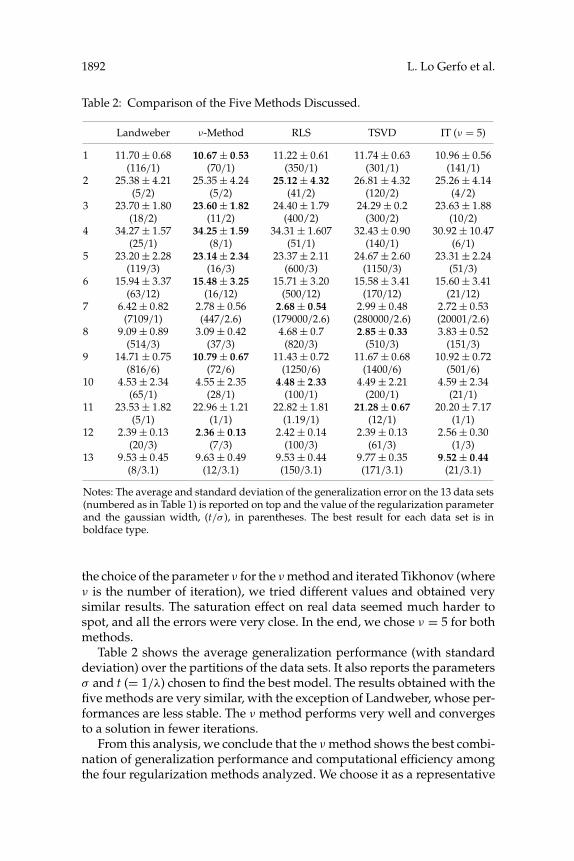
Table 2: Comparison of the Five Methods Discussed.

Landweber ν-Method RLS TSVD IT (ν = 5)

1 11.70 ± 0.68 10.67 ± 0.53 11.22 ± 0.61 11.74 ± 0.63 10.96 ± 0.56(116/1) (70/1) (350/1) (301/1) (141/1)

2 25.38 ± 4.21 25.35 ± 4.24 25.12 ± 4.32 26.81 ± 4.32 25.26 ± 4.14(5/2) (5/2) (41/2) (120/2) (4/2)

3 23.70 ± 1.80 23.60 ± 1.82 24.40 ± 1.79 24.29 ± 0.2 23.63 ± 1.88(18/2) (11/2) (400/2) (300/2) (10/2)

4 34.27 ± 1.57 34.25 ± 1.59 34.31 ± 1.607 32.43 ± 0.90 30.92 ± 10.47(25/1) (8/1) (51/1) (140/1) (6/1)

5 23.20 ± 2.28 23.14 ± 2.34 23.37 ± 2.11 24.67 ± 2.60 23.31 ± 2.24(119/3) (16/3) (600/3) (1150/3) (51/3)

6 15.94 ± 3.37 15.48 ± 3.25 15.71 ± 3.20 15.58 ± 3.41 15.60 ± 3.41(63/12) (16/12) (500/12) (170/12) (21/12)

7 6.42 ± 0.82 2.78 ± 0.56 2.68 ± 0.54 2.99 ± 0.48 2.72 ± 0.53(7109/1) (447/2.6) (179000/2.6) (280000/2.6) (20001/2.6)

8 9.09 ± 0.89 3.09 ± 0.42 4.68 ± 0.7 2.85 ± 0.33 3.83 ± 0.52(514/3) (37/3) (820/3) (510/3) (151/3)

9 14.71 ± 0.75 10.79 ± 0.67 11.43 ± 0.72 11.67 ± 0.68 10.92 ± 0.72(816/6) (72/6) (1250/6) (1400/6) (501/6)

10 4.53 ± 2.34 4.55 ± 2.35 4.48 ± 2.33 4.49 ± 2.21 4.59 ± 2.34(65/1) (28/1) (100/1) (200/1) (21/1)

11 23.53 ± 1.82 22.96 ± 1.21 22.82 ± 1.81 21.28 ± 0.67 20.20 ± 7.17(5/1) (1/1) (1.19/1) (12/1) (1/1)

12 2.39 ± 0.13 2.36 ± 0.13 2.42 ± 0.14 2.39 ± 0.13 2.56 ± 0.30(20/3) (7/3) (100/3) (61/3) (1/3)

13 9.53 ± 0.45 9.63 ± 0.49 9.53 ± 0.44 9.77 ± 0.35 9.52 ± 0.44(8/3.1) (12/3.1) (150/3.1) (171/3.1) (21/3.1)

Notes: The average and standard deviation of the generalization error on the 13 data sets(numbered as in Table 1) is reported on top and the value of the regularization parameterand the gaussian width, (t/σ ), in parentheses. The best result for each data set is inboldface type.

the choice of the parameter ν for the ν method and iterated Tikhonov (whereν is the number of iteration), we tried different values and obtained verysimilar results. The saturation effect on real data seemed much harder tospot, and all the errors were very close. In the end, we chose ν = 5 for bothmethods.

Table 2 shows the average generalization performance (with standarddeviation) over the partitions of the data sets. It also reports the parametersσ and t (= 1/λ) chosen to find the best model. The results obtained with thefive methods are very similar, with the exception of Landweber, whose per-formances are less stable. The ν method performs very well and convergesto a solution in fewer iterations.

From this analysis, we conclude that the ν method shows the best combi-nation of generalization performance and computational efficiency amongthe four regularization methods analyzed. We choose it as a representative


Table 3: Comparison of the ν Method Against the Best of the Seven MethodsTaken from the Benchmark Web Page on the Benchmark Data Sets.

Best of Seven SVM ν-Method

Banana LP REG-Ada10.73 ± 0.43 11.53 ± 0.66 10.67 ± 0.53

Breast Cancer KFD24.77 ± 4.63 26.04 ± 4.74 25.35 ± 4.24

Diabetes KFD23.21 ± 1.63 23.53 ± 1.73 23.60 ± 1.82

Flare Solar SVM-RBF32.43 ± 1.82 32.43 ± 1.82 34.25 ± 1.59

German SVM-RBF23.61 ± 2.07 23.61 ± 2.07 23.14 ± 2.08

Heart SVM-RBF15.95 ± 3.26 15.95 ± 3.26 15.48 ± 3.25

Image ADA REG2.67 ± 0.61 2.96 ± 0.6 2.78 ± 0.56

Ringnorm ADA REG1.58 ± 0.12 1.66 ± 0.2 3.09 ± 0.42

Splice ADA REG9.50 ± 0.65 10.88 ± 0.66 10.79 ± 0.67

Thyroid KFD4.20 ± 2.07 4.80 ± 2.19 4.55 ± 2.35

Titanic SVM-RBF22.42 ± 1.02 22.42 ± 1.02 22.96 ± 1.21

Twonorm KFD2.61 ± 0.15 2.96 ± 0.23 2.36 ± 0.13

Waveform KFD9.86 ± 0.44 9.88 ± 0.44 9.63 ± 0.49

Note: The middle column shows the results for SVM from the same Web page.

for comparisons with other approaches. Table 3 compares the results ob-tained with the ν method with an SVM with RBF kernel and, for eachdata set, with the classifier performing best among the seven methods con-sidered on the benchmark page (including RBF networks, AdaBoost andRegularized AdaBoost, Kernel Fisher Discriminant, and SVMs with RBFkernels). The results obtained with the ν method compare favorably withthe ones achieved by the other methods.

7.2 Experiments on Face Detection. This section reports the analysiswe carried out on the problem of face detection in order to evaluate theeffectiveness of the ν method in comparison to SVMs. The structure ofthe experiments, including model selection and error estimation, follows theone reported above. The data we consider are image patches. We representthem in the simplest way, unfolding the patch matrix in a one-dimensionalvector of integer values—the gray levels. All the images of the two data setsare 19 × 19; thus, the size of our data is 361.


Table 4: Average and Standard Deviation of the Classification Error of SVMand ν-Method Trained on Training Sets of Increasing Size.

Number Trained PlusNumber TestedClassifier 600 + 1400 700 + 1300 800 + 1200

RBF-SVM 2.41 ± 1.39 1.99 ± 0.82 1.60 ± 0.71σ = 800 C = 1 σ = 1000 C = 0.8 σ = 1000 C = 0.8

ν-method 1.63 ± 0.32 1.53 ± 0.33 1.48 ± 0.34σ = 341 t = 85 σ = 341 t = 89 σ = 300 t = 59

Note: The data are the CBCL-MIT benchmark data set of frontal faces (see text).

The first data set we used for training and testing is the well-known CBCLdata set for frontal faces composed of thousands of small images of positiveand negative examples of size (available online at http://cbcl.mit.edu/software-datasets/FaceData2.html). The face images obtained from thisbenchmark are clean and nicely registered.

The second data set we consider is made of low-quality images acquiredby a monitoring system installed in our department (the data set is avail-able on request). The data are very different from the previous set sincethey have been obtained from video frames (therefore, they are noisy andoften blurred by motion), faces have not been registered, and gray valueshave not been normalized. The RBF kernel may take into account slightdata misalignment due to the intraclass variability, but in this case, modelselection is more crucial, and the choice of an appropriate parameter for thekernel is advisable.

The experiments performed on these two sets follow the structure dis-cussed in the previous section. Starting from the original set of data, in bothcases we randomly extracted 2000 data that we use for most of our experi-ments: for a fixed training set size, we generate 50 resamplings of trainingand test data. Then we vary the training set size from 600 (300 + 300) to 800(400 + 400) training examples. The results obtained are reported in Tables 4and 5. The tables show a comparison between the ν method and SVM asthe size of the training set grows. The results obtained are slightly different:while on the CBCL data set the ν method performance is clearly above theSVM classifier, in the second set of data, the performance of the ν methodincreases as the training set size grows.

At the end of this evaluation process, we retrained the ν-method on thefull set of 2000 data and again tuned the parameters with KCV, obtainingσ = 200 and t = 58. Then we used this classifier to test a batch of newlyacquired data (the size of this new test set is of 6000 images), obtaining aclassification error of 3.67%. These results confirm the generalization abilityof the algorithm. For completeness, we report that the SVM classifier trainedand tuned on the entire data set (σ = 600 and C = 1) leads to an error rateof 3.92%.


Table 5: Average and Standard Deviation of the Classification Error of SVMand ν-Method Trained on Training Sets of Increasing Size.

Number Trained PlusNumber TestedClassifier 600 + 1400 700 + 1300 800 + 1200

RBF-SVM 3.99 ± 1.21 3.90 ± 0.92 3.8 ± 0.58σ = 570 C = 2 σ = 550 C = 1 σ = 550 C = 1

ν-method 4.36 ± 0.53 4.19 ± 0.50 3.69 ± 0.54σ = 250 t = 67 σ = 180 t = 39 σ = 200 t = 57

Note: The data have been acquired by a monitoring system developed in our laboratory(see text).

8 Conclusion

In this letter, we present and discuss several spectral algorithms for su-pervised learning. Starting from the standard regularized least squares,we show that a number of methods from inverse problems theory lead toconsistent learning algorithms. We provide a unifying theoretical analy-sis based on the concept of filter function showing that these algorithms,which differ from the computational viewpoint, are all consistent ker-nel methods. The iterative methods, like the ν method and the iterativeLandweber, and projections methods, like spectral cut-off or PCA, give riseto regularized learning algorithms in which the regularization parameteris the number of iterations or the number of dimensions in the projection,respectively.

We report an extensive experimental analysis on a number of data setsshowing that all the proposed spectral algorithms are a good alternative,in terms of generalization performances and computational efficiency, tostate-of-the-art algorithms for classification like SVM and AdaBoost. Oneof the main advantages of the methods we propose is their simplicity: eachspectral algorithm is an easy-to-use linear method whose implementationis straightforward. Indeed, our experience suggests that this helps deal-ing with overfitting in a transparent way and makes the model selectionstep easier. In particular, the search for the best choice of the regulariza-tion parameter in iterative schemes is naturally embedded in the iterationprocedure.

Acknowledgments

We thank S. Pereverzev for useful discussions and suggestions and A.Destrero for providing the faces data set. This work has been partiallysupported by the FIRB project LEAP RBIN04PARL and by the EU IntegratedProject Health-e-Child IST-2004-027749.


References

Aronszajn, N. (1950). Theory of reproducing kernels. Trans. Amer. Math. Soc., 68,337–404.

Bartlett, P. L., Jordan, M. I., & McAuliffe, J. D. (2006). Convexity, classification, andrisk bounds. J. Amer. Statist. Assoc., 101(473), 138–156.

Bauer, F., Pereverzev, S., & Rosasco, L. (2007). On regularization algorithms in learn-ing theory. Journal of Complexity, 1, 52–72.

Bertero, M., & Boccacci, P. (1998). Introduction to inverse problems in imaging. Bristol:IOP Publishing.

Bousquet, O., & Elisseeff, A. (2002). Stability and generalization. Journal of MachineLearning Research, 2, 499–526.

Buhlmann, P., & Yu, B. (2002). Boosting with the l2-loss: Regression and classification.Journal of American Statistical Association, 98, 324–340.

Caponnetto, A. (2006). Optimal rates for regularization operators in learning theory(Tech. Rep. CBCL Paper 264/CSAIL-TR 2006-062). Cambridge, MA: MIT. Avail-able online at http://cbcl.mit.edu/projects/cbcl/publications/ps/MIT-CSAIL-TR-2006-062.pdf.

Caponnetto, A., & De Vito, E. (2007). Optimal rates for regularized least-squaresalgorithm. Found. Comput. Math., 3, 331–368.

Chapelle, O., Weston, J., & Scholkopf, B. (2003). Cluster kernels for semisupervisedlearning. In S. Becker, S. Thrun, & K. Obermayer (Eds.), Neural information pro-cessing systems, 15 (pp. 585–592). Cambridge, MA: MIT Press.

De Vito, E., Caponnetto, A., & Rosasco, L. (2005). Model selection for regularizedleast-squares algorithm in learning theory. Found. Comput. Math., 5(1), 59–85.

De Vito, E., Rosasco, L., & Caponnetto, A. (2006). Discretization error analysis forTikhonov regularization. Anal. Appl., 4(1), 81–99.

De Vito, E., Rosasco, L., Caponnetto, A., De Giovannini, U., & Odone, F. (2005). Learn-ing from examples as an inverse problem. Journal of Machine Learning Research, 6,883–904.

De Vito, E., Rosasco, L., & Verri, A. (2005). Spectral methods for regularization in learningtheory (Tech. Rep.). DISI, Universita degli Studi di Genova, Italy.

Engl, H. W., Hanke, M., & Neubauer, A. (1996). Regularization of inverse problems.Dordrecht: Kluwer Academic.

Evgeniou, T., Pontil, M., & Poggio, T. (2000). Regularization networks and supportvector machines. Adv. Comp. Math., 13, 1–50.

Girosi, F., Jones, M., & Poggio, T. (1995). Regularization theory and neural networksarchitectures. Neural Computation, 7(2), 219–269.

Golub, G. H., & Van Loan, C. F. (1996). Matrix computations (3rd ed.). Baltimore, MD:Johns Hopkins University Press.

Hastie, S. T., Rosset, S., Tibshirani, R., & Zhu, J. (2004). The entire regularization pathfor the support vector machine. JMLR, 5, 1391–1415.

Hastie, T., Tibshirani, R., & Friedman, J. (2001). The elements of statistical learning. NewYork: Springer.

Li, W., Lee, K.-H., & Leung, K.-S. (2007). Large-scale RLSC learning without agony.In ICML ’07: Proceedings of the 24th International Conference on Machine Learning(pp. 529–536). New York: ACM Press.


Micchelli, C. A., Xu, Y., & Zhang, H. (2006). Universal kernels. JMLR, 7, 2651–2667.Ong, C., & Canu, S. (2004). Regularization by early stopping (Tech. Rep.). Computer

Sciences Laboratory and RSISE, Australian National University. Available onlineat http://asi.insa-rouen.fr/scanu/.

Ong, C., Mary, X., Canu, S., & Smola, A. (2004). Learning with nonposi-tive kernels. In Proceedings of the 21st International Conference on MachineLearning. New York: ACM Press. Available online at http://www.aicml.cs.ualberta.ca/ banff04/icml/pages/papers/392.pdf.

Poggio, T., & Girosi, F. (1992). A theory of networks for approximation and learning.In C. Lau (Ed.), Foundation of neural networks (pp. 91–106). Piscataway, NJ: IEEEPress.

Poggio, T., Rifkin, R., Mukherjee, S., & Niyogi, P. (2004). General conditions forpredictivity in learning theory. Nature, 428, 419–422.

Pontil, M., & Verri, A. (1998). Properties of support vector machines. Neural Compu-tation, 10, 977–996.

Rakhlin, A., Mukherjee, S., & Poggio, T. (2005). Stability results in learning theory.Analysis and Applications, 3, 397–419.

Scholkopf, B., & Smola, A. (2002). Learning with kernels. Cambridge, MA: MIT Press.Smale, S., & Zhou, D.-X. (2004). Shannon sampling and function reconstruction from

point values. Bull. Amer. Math. Soc. (N.S.), 41(3), 279–305.Smale, S., & Zhou, D.-X. (2005). Shannon sampling. II. Connections to learning theory.

Appl. Comput. Harmon. Anal., 19(3), 285–302.Smale, S., & Zhou, D.-X. (2007). Learning theory estimates via integral operators and

their approximations. Constructive Approximation, 26(2), 153–172.Smola, A., & Kondor, R. (2003). Kernels and regularization on graphs. In Learning

theory and kernel machines. Berlin: Springer-Verlag.Tikhonov, A., & Arsenin, V. (1977). Solutions of ill posed problems. Washington, DC:

Winston.Vapnik, V. (1982). Estimation of dependences based on empirical data. New York: Springer-

Verlag.Vapnik, V. N. (1998). Statistical learning theory. New York: Wiley.Wahba, G. (1990). Spline models for observational data. Philadelphia: SIAM.Wu, Q., Ying, Y., & Zhou, D.-X. (2006). Learning rates of least-square regularized

regression. Found. Comput. Math., 6(2), 171–192.Yao, Y., Rosasco, L., & Caponnetto, A. (2007). On early stopping in gradient descent

learning. Constructive Approximation, 26, 289–315.Zhang, T., & Ando, R. (2006). Analysis of spectral kernel design based semi-

supervised learning. In Y. Weiss, B. Scholkopf, & J. Platt (Eds.), Advances in neuralinformation processing systems, 18 (pp. 1601–1608). Cambridge, MA: MIT Press.

Zhu, X., Kandola, J., Ghahramani, Z., & Lafferty, J. (2005). Nonparametric transformsof graph kernels for semi-supervised learning. In L. K. Saul, Y. Weiss, & L. Bottou(Eds.), Neural information processing systems, 17. Cambridge, MA: MIT Press.

Received May 9, 2007; accepted October 30, 2007.

spectral algorithms for supervised learning - dimadevito/pub_con/spectralneco.pdfspectral algorithms...

Documents