working paper

department

of economics

SPECIFICATION TESTS IN ECONOMETRICS

J. A. Hausman

Number 185

•MASS. INS i.TSCH

OCT 13 1975

June 1976

Revised August 1976

massachusetts

institute of

technology

50 memorial drive

Cambridge, mass. 02139

SPECIFICATION TESTS IN ECONOMETRICS

J. A. Hausman

MA3S.lN3i.T; r;

J

OCT 13 1975

Number 185

DEWEY LIBRARY

June 1976Revised August 1976

I would like to thank D, W. Carlton, G. Chamberlain, F. M. Fisher,R, H. Gordon, R. E, Hall, and R, L. White for helpful discussions.A. S. Kelso and E. R. Rosenthal provided research assistance.Research support has been provided by the NSF.

The views expressed in this paper are the author's sole responsibilityand do not reflect those of the Department of Economics, the MassachusettsInstitute of Technology, or the National Science Foundation.

Digitized by the Internet Archive

in 2011 with funding from

Boston Library Consortium Member Libraries

http://www.archive.org/details/specificationtesOOhaus

1. Introduction

Specification tests form one of the most important areas for research

in econometrics. In the standard regression framework, y = X$ + e, the

two stochastic specifications are first that e is independent of X (or

for fixed X, £ has expectation zero) and that e has a spherical covariance

matrix

(1.1) a. E(e|x) =

b. V(e|x) = a2I

Failure of the first assumption, sometimes called the orthogonality

assumption, leads to biased estimates while failure of the second assump-

tions, sometimes called the sphericality assumption, leads to loss of

efficiency although the central tendency of the estimator is still correct.

While in many problems the payoff to detecting failure of assumption (1.1. a.)

is presumably greater than detecting failure of assumption (l.l.b.), most

of the attention in the econometric literature has been paid to devising

tests for the latter assumption. Theil's [1957] famous specification test

for left out variables is almost the only exception. Yet, the problem is

so important that increased attention should be paid, especially since

efficient estimators are now used in almost all situations; and these

estimators are often quite sensitive to failures of the first assumption.

In this paper a general form of specification test is proposed which

attempts to provide powerful tests of assumption (1.1. a.). A main stumbling

block to specification tests has been a lack of precisely specified

alternative hypotheses. Here, I point out that in many situations, in-

cluding time series - cross section specifications, errors in variables

7^5H

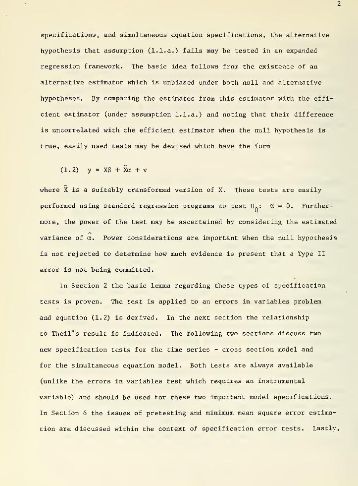
specifications, and simultaneous equation specifications, the alternative

hypothesis that assumption (1.1. a.) fails may be tested in an expanded

regression framework. The basic idea follows from the existence of an

alternative estimator which is unbiased under both null and alternative

hypotheses. By comparing the estimates from this estimator with the effi-

cient estimator (under assumption 1.1. a.) and noting that their difference

is uncorrelated with the efficient estimator when the null hypothesis is

true, easily used tests may be devised which have the form

(1.2) y = XB + Xa + v

where X is a suitably transformed version of X. These tests are easily

performed using standard regression programs to test H_: a = 0. Further-

more, the power of the test may be ascertained by considering the estimated

variance of a. Power considerations are important when the null hypothesis

is not rejected to determine how much evidence is present that a Type II

error is not being committed.

In Section 2 the basic lemma regarding these types of specification

tests is proven. The test is applied to an errors in variables problem

and equation (1.2) is derived. In the next section the relationship

to Theil's result is indicated. The following two sections discuss two

new specification tests for the time series - cross section model and

for the simultaneous equation model. Both tests are always available

(unlike the errors in variables test which requires an instrumental

variable) and should be used for these two important model specifications.

In Section 6 the issues of pretesting and minimum mean square error estima-

tion are discussed within the context of specification error tests. Lastly,

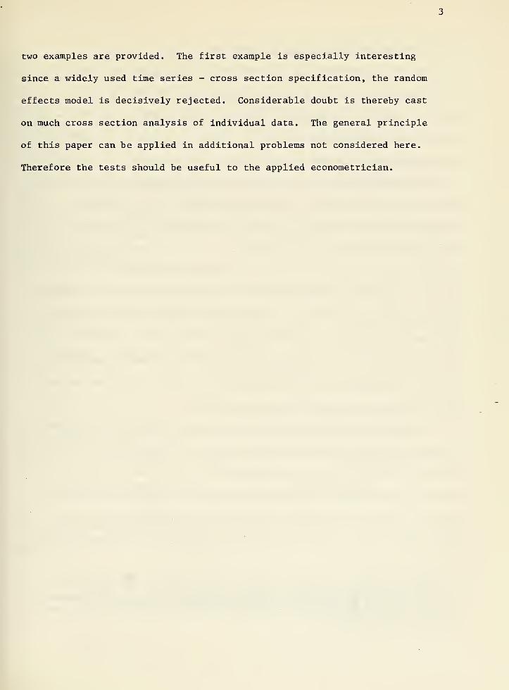
two examples are provided. The first example is especially interesting

since a widely used time series - cross section specification, the random

effects model is decisively rejected. Considerable doubt is thereby cast

on much cross section analysis of individual data. The general principle

of. this paper can be applied in additional problems not considered here.

Therefore the tests should be useful to the applied econometrician.

2. Theory and a Test of Errors in Variables

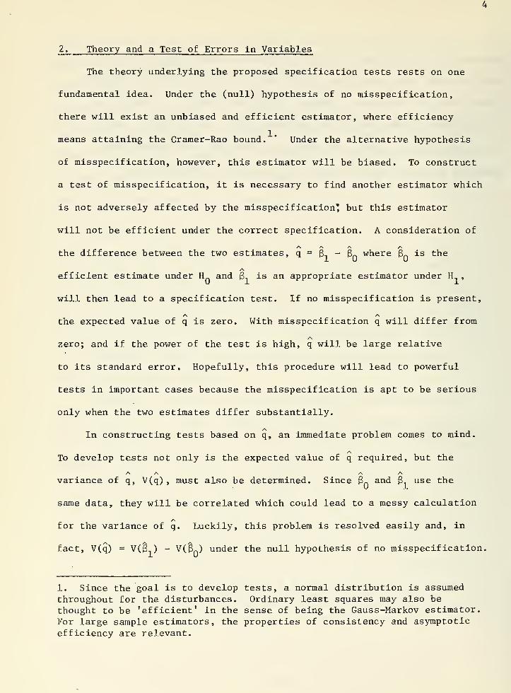
The theory underlying the proposed specification tests rests on one

fundamental idea. Under the (null) hypothesis of no misspecification,

there will exist an unbiased and efficient estimator, where efficiency

means attaining the Cramer-Rao bound. ' Under the alternative hypothesis

of misspecification, however, this estimator will be biased. To construct

a test of misspecif ication, it is necessary to find another estimator which

is not adversely affected by the misspecif ication* but this estimator

will not be efficient under the correct specification. A consideration of

the difference between the two estimates, q = $-1 - $ where 3nis the

efficient estimate under Hn and 3-. is an appropriate estimator under H-. ,

will then lead to a specification test. If no misspecification is present,

the expected value of q is zero. With misspecif ication q will differ from

zero; and if the power of the test is high, q will be large relative

to its standard error. Hopefully, this procedure will lead to powerful

tests in important cases because the misspecif ication is apt to be serious

only when the two estimates differ substantially.

In constructing tests based on q, an immediate problem comes to mind.

To develop tests not only is the expected value of q required, but the

variance of q, V(q) , must also be determined. Since 3n and 3., use the

same data, they will be correlated which could lead to a messy calculation

for the variance of q. Luckily, this problem is resolved easily and, in

fact, V(q) = V( 3-. ) - v (i3(0 under the null hypothesis of no misspecif ication.

1. Since the goal is to develop tests, a normal distribution is assumedthroughout for the disturbances. Ordinary least squares may also bethought to be 'efficient' in the sense of being the Gauss-Markov estimator.

For large sample estimators, the properties of consistency and asymptoticefficiency are relevant.

Thus, the construction of specification error tests is simplified since

the estimators may be considered separately without regard to their in-

teraction. The intuitive reasoning behind this result is simple although

it appears to have remained unnoticed in the general case. The idea rests

on the fact that the efficient estimator, 6 , must be uncorrelated with

q under the null hypothesis for any other unbiased estimator 3, . If this

were not the case, a linear combination of 3nand q could be taken which

would lead to an unbiased estimator B. which would have smaller variance

than $„ which is assumed efficient. To prove the result formally, consider

the following lemma:

/\ /\

(2.1) Lemma : Consider two estimators 3n , 3, which are both unbiased

and normally distributed with 3nattaining the Cramer-Rao bound

(alternatively, both consistent and asymptotically normal with 3~

/\ /\

attaining the CR bound asymptotically '). Consider q = 3, - 3Q

.

/s. /\

Then 3nand q have zero covariance, C(3 , q) = 0.

Proof: Suppose 3nand q are not orthogonal. Since Eq = define

a new estimator 3?

= Bn+ rAq where r is a scalar and A is an arbitrary

matrix to be chosen. The new estimator is unbiased and normal with variance

(2.2) V(32) = V(3

Q) + rAC(3

Q , q) + rC(3Q , q)A' + r

2AV(q)A'

.

Now consider the difference between the variance of the new estimator

and the old efficient estimator

1. Besides consistency and asymptotic normality, uniform convergenceis also required to rule out superef ficiency. See Rao [1973» P- 284].

(2.3) F(r) = V(62) - V(3

Q) = rAC + rCA* + r

2AV(q)A'

Taking derivatives with respect to r yields

(2. A) F'(r) = AC + CA* + 2rAV(q)A'.

Then choose A = -C' and noting that C is symmetric leads to

(2.5) F'(r) = -2C'C + 2rC'V(q)C.

Therefore at r = 0, F'(0) = -2C'C < in the sense of being nonpositive

definite. But F(0) = so for r small there is a contradiction unless

C = C(Bn , q) = since 3n is efficient.

Once it has been shown that the efficient estimator is uncorrelated

with q, the variance of q is easily calculated.

/\ /\ y\

(2.6) Corollary : V(q) = V(3-.) - V(6n ) > in the sense of being nonnegative

definite.

/\ /\

Proof: Since q + 3Q

= 3,, V(q) + V(3Q

) = V(3,)- Furthermore,

3„ attains the CR bound.

Given this result a general misspecif ication test can be specified by

considering the statistic

(2.7) m = q'V(q)1q ^ KF

K,T-K

where K is the number of unknown parameters in 3, and F is distributed as

Snedecor's central F distribution with K and T-K degrees of freedom when no

misspecification is present.

1. In forming V(q) the estimate of O used must be independent of q for

m to be distributed exactly as F. To insure this property and also for

2the analysis of the noncentral F considered below the estimate of O

/-, 2 ^from 3-, , s , is used. For the case where other elements of V(q) are

estimated, e.g., the simultaneous equation problem of section 5, then2

large sample properties are used and m is distributed as v •

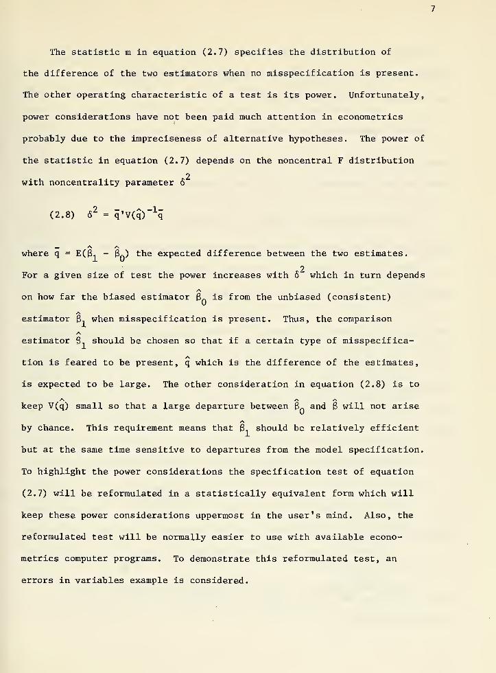
The statistic m in equation (2.7) specifies the distribution of

the difference of the two estimators when no misspecification is present.

The other operating characteristic of a test is its power. Unfortunately,

power considerations have not been paid much attention in econometrics

probably due to the impreciseness of alternative hypotheses. The power of

the statistic in equation (2.7) depends on the noncentral F distribution

2with noncentrality parameter 6

(2.8) S2

= q'V(q)-1

q

where q = E(3i - 3n ) the expected difference between the two estimates.

2For a given size of test the power increases with 6 which in turn depends

on how far the biased estimator $nis from the unbiased (consistent)

estimator 3-, when misspecif ication is present. Thus, the comparison

estimator $ should be chosen so that if a certain type of misspecif ica-

tion is feared to be present, q which is the difference of the estimates,

is expected to be large. The other consideration in equation (2.8) is to

keep V(q) small so that a large departure between 3nand 3 will not arise

by chance. This requirement means that 3-, should be relatively efficient

but at the same time sensitive to departures from the model specification.

To highlight the power considerations the specification test of equation

(2.7) will be reformulated in a statistically equivalent form which will

keep these power considerations uppermost in the user's mind. Also, the

reformulated test will be normally easier to use with available econo-

metrics computer programs. To demonstrate this reformulated test, an

errors in variables example is considered.

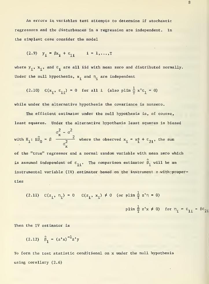
An errors in variables test attempts to determine if stochastic

regressors and the disturbances in a regression are independent. In

the simplest case consider the model

(2.9) y±= 3x

±+ e

lii - 1 T

where v., x., and e. are all iid with mean zero and distributed normally.

Under the null hypothesis, x. and r\. are independent

(2.10) C(x., e ) = for all i (also plim -^ x'e = 0)

while under the alternative hypothesis the covariance is nonzero.

The efficient estimator under the null hypothesis is, of course,

least squares. Under the alternative hypothesis least squares is biased

2 2a - ax

2with H-. : EBn

= 3 5 where the observed x. = x* + £„., the sumaX

of the "true" regressor and a normal random variable with mean zero which

is assumed independent of £.. . . The comparison estimator 3, will be an

instrumental variable (IV) estimator based on the instrument z with proper-

ties

(2.11) C(z±

, n±) = C( Z;L , x

±) * (or plim ^ z'n = 0)

plim — z'x ^ 0) for T). = £.. . - 3e2

-

Then the IV estimator is

(2.12) g1

= (z'x)_1

z'y

To form the test statistic conditional on x under the null hypothesis

using corollary (2.6)

/\ S\

(2.13) q = Bx- B

Q~ N(0, B)

2 ~ ^ —i -1 ~ -1where B = V(q) = a [(x'x) - (x'x) ] where x = z(z'z) z'x. Again

/s _]_* 2using the corollary q'B q is distributed as X-, • To derive an F test

2 2use s

1the IV estimator of to form B. Then the test of misspecification

is

(2.14) m = q*B_1

q ^ ^ ^2 2 2

Choice of an alternative estimate of o , say s^ the OLS estimate of a ,

2leads to a similar test which is distributed as X-i in large samples

under the null hypothesis. * The large sample approximation to the power

of the test depends primarily on the numerator of equation (2.14) as shown

- 2 2in equation (2.8). Under H

1, the expected value of q, q = 3'Cf /a so the

power depends on the magnitude of the two coefficients and the correlation

of the right hand side variable with the disturbance. To compute the

power as a function of 3, equation (2.8) can be used. The IV estimates,

" 2BT„ and s

1, are unbiased under both the null and alternative hypotheses

/v 2as is V(q) . An unbiased estimate of O follows from the data using

2the formula for the sample variance, and an estimate of cr is derived

2/%2 "" A y%2 —

from the equation = (1 - 3mc /6T„)<7 . Then q may be calculated forc-n ULiO i.V X^

2any choice of 3 and the noncentrality parameter 6 is a quadratic function

around 3 - 0, 6 = (3 /o V(q)). The tables of the noncentral F test2

X

in Scheffe [1959] can be consulted to find the probability of the null

hypothesis being rejected for a given value of 3 if the alternative

1. Under the alternative hypothesis, the power of the test is difficult

to analyze since B is now an inconsistent estimate of B.

10

hypothesis is true conditional on the estimates of the incidental param-

eters of the problem. This type of IV (instrumental variable) tests for

errors in variables was first proposed by Liviatan [1963]. Wu [1973]

generalizes the test and considers tests with different estimates of the

2nuisance parameter a . He also calculates the power of the different

tests.

The IV test for errors in variables is known in the literature,

but an alternative formulation of test leads to easier implementation.

Also, the alternative formulation demonstrates the general format of mis-

specification tests. Consider the regression specification with 2 arbitrary

scalar parameters B and a

(2.15) y = x3 + xa + v.

where as before x = z(z'z) z'x=Px. Define Q = I-P where P = x(x'x) x'z x x x

and project the model of equation (2.15) into the subspace orthogonal to x

(2.16) Qxy = Qx

xg + O^xCX + Q^v

Taking expectations of equation (2.16) under the null hypothesis where

from equation (2.9), EQ y = y - x3 and EQ xB = 0,X A

(2.17) Ey = xB + 0^:xa.

1. The instrumental variable test can also be considered a formalizationand an improvement of a suggestion by Sargan [ ] who recommended checkingwhether the least squares estimates lie outside the confidence regionsof the IV estimates. For individual coefficients the procedure used here

is to see whether the least squares estimate lies outside the confidenceregions centered at the IV estimate and with length formed from the square

root of the difference of the IV variance minus the OLS variance. Thus

shorter confidence intervals follow from the current procedure than from

Sargan' s suggestion. The F test on all the coefficients in equation

(2.14), however, is the preferred test of the null hypothesis rather than

separate consideration of each confidence interval.

11

so that the expectation of the second term should be zero if the null

hypothesis is true. Then estimating a from using OLS on equation (2.15)

leads to an estimate

(2.18) aQ

= (x'Q^xr^'Q^.

A test of a = from equation (2.17) under the null hypothesis is then

based on the statistic a x = a'(x'Q x)aQ

. But — (x'Q x)~ =

(x'x) B (x x) and a = (x'Q x) (x'x)q. Thus, this formulation is

equivalent to the IV test of equation (2.14) since

(2.19)^2

a (x,Qxx)a =

2 I'^'^^'V5 <X '*)<1

= q'B q.

A simple t-test on a on the OLS estimate a from equation (2.15) yields

a test on whether errors in variables is present and is equivalent to

2the large sample test using s_ under the null hypothesis since equation

(2.17) shows that a equals zero under the null hypothesis of no errors

in variables. Besides ease of computation another advantage is present.

Three outcomes of the test will be encountered leading to simple power

interpretations which may not be as evident using the previous formulation

of the test. First, ot may be large relative to its standard error. This

result points to rejection of the hypothesis of no misspecif ication. The

other clear cut case is a small a with a small standard error which pre-

sents little evidence against H_. The last result is a large standard

error relative to the size of ol. This finding points to lack of power of

the test and arises when x and x in equation (2.15) are "multicollinear"

leading to a small (x Q x) . If z is not a very good instrument because it

12

is not highly correlated with x, then the estimated standard error will be

large relative to cL. The lack of power will be very evident to the user

since he will not have a precise estimate of a.

Two immediate generalizations of the errors in variables specification

test can be made. The test can be used to test any potential failure

of Assumption (1.1. a.) that the right hand side variables are orthogonal

to the error term so long as instrumental variables are available. First,

additional right hand side variables can be present

(2.20) y = X±$1+ X

2e2+ e.

where the X.. variables are possibly correlated with e while the X„ variables

are known to be uncorrelated. Given a matrix of variables Z (which should

include X ) , q will again be the difference between the IV estimator

and the efficient OLS estimator. Letting X = P„X1

leads to the regression

(2.21) y = X1B1+ X

262+ X

xa + v

where a test of L: a = is a test for errors in variables. The last

orthogonality test involves a lagged endogenous variable which may be

correlated with the disturbance. In this case, however, if the specification

of the error process is known such as first order serial correlation, a

1.more powerful test may be available.'

1. For the true regression problem (no lagged endogenous variables)

under both the null hypothesis of no serial correlation and the alternative

hypothesis 3 , the OLS estimator, is unbiased since only Assumption

l.l.b. is violated. Therefore, if the null hypothesis of serial correla-

tion is tested with an autoregressive estimator B-. , Eq = q = under

both hypotheses. If q is large relative to its standard error, misspecifica-

tion is likely to be present.

13

In this section the general nature of the misspecif ication problem has

been discussed when there exists an alternative estimator which provides

consistent estimates under misspecif ication. By demonstrating that the

efficient estimator is uncorrelated with the difference between the con-

sistent and efficient estimator, a simple expression for the variance of

the test is found. Then by applying it to the errors in variables problem,

a very easy method to apply the test is demonstrated which also makes power

considerations clearer. Before going on to discuss additional specifica-

tion tests, "the" original specification test of Theil is discussed, and

the current approach is shown to be a generalization of Theil' s analysis.

14

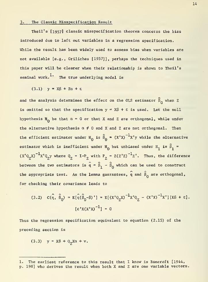
3. The Classic Misspecif ication Result

Theil's [1957] classic misspecif ication theorem concerns the bias

introduced due to left out variables in a regression specification.

While the result has been widely used to assess bias when variables are

not available [e.g., Griliches [1957]], perhaps the techniques used in

this paper will be clearer when their relationship is shown to Theil's

seminal work. " The true underlying model is

(3.1) y = XB + Za + e

and the analysis determines the effect on the OLS estimator Bnwhen Z

is omitted so that the specification y = XB + £ is used. Let the null

hypothesis H_ be that a = or that X and Z are orthogonal, while under

the alternative hypothesis a ^ and X and Z are not orthogonal. Then

/v -1the efficient estimator under Hn is Bn

= (X'X) X'y while the alternative

estimator which is inefficient under Hn

but unbiased under H is B, =

(X'Q X)_1X'Q y where Q = I-P with P = Z(Z , Z)~

1Z'. Thus, the difference

Zi Zi Cm Lt Li

/\ /\

between the two estimators is q = B-, - 3nwhich can be used to construct

the appropriate test. As the lemma guarantees, q and Bnare orthogonal,

for checking their covariance leads to

(3.2) C(q, 6 ) = E[q(3Q-3)'] = E[ (X'Q

ZX)

_1X'Q

Z- (X'X)

_1X' ] [XB + e]

[e , X(X'X)~1

]=

Thus the regression specification equivalent to equation (2.15) of the

preceding section is

(3.3) y = XB + Q„Xa + v.L*

1. The earliest reference to this result that I know is Bancroft [1944,

p. 198] who derives the result when both X and Z are one variable vectors,

15

The test of a = from this regression is then equivalent to testing

whether bias will be introduced due to Theil's misspecif ication theorem.

This misspecif ication test is often difficult to apply because ob-

servations on Z are not available either because data has not been col-

lected or because Z is an unobservable variable. The next misspecification

test, however, always can be done since the necessary data is available.

It is a test on the random effects model which has been widely used in

econometrics.

16

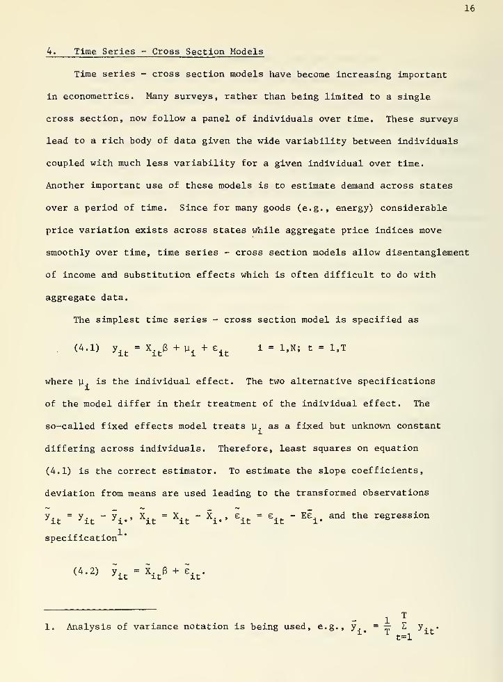
4. Time Series - Cross Section Models

Time series - cross section models have become increasing important

in econometrics. Many surveys, rather than being limited to a single

cross section, now follow a panel of individuals over time. These surveys

lead to a rich body of data given the wide variability between individuals

coupled with much less variability for a given individual over time.

Another important use of these models is to estimate demand across states

over a period of time. Since for many goods (e.g., energy) considerable

price variation exists across states while aggregate price indices move

smoothly over time, time series - cross section models allow disentanglement

of income and substitution effects which is often difficult to do with

aggregate data.

The simplest time series - cross section model is specified as

(4.1) y.t

= X±t

B + V±+ e

±ti = 1,N; t = 1,T

where u. is the individual effect. The two alternative specifications

of the model differ in their treatment of the individual effect. The

so-called fixed effects model treats U . as a fixed but unknown constanti

differing across individuals. Therefore, least squares on equation

(4.1) is the correct estimator. To estimate the slope coefficients,

deviation from means are used leading to the transformed observations

yit= yit

" yi-'Xit

= Xit

" V* £it

= eit

~ Eii-

and the re§ression

... .. 1.specification

(4.2) y.t= X.

t3 + e

lt.

T1

i

1. Analysis of variance notation is being used, e.g., y. = — £ y-*-'1 * l

t=l

17

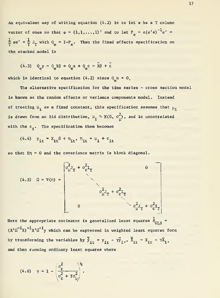
An equivalent way of writing equation (4.2) is to let e be a T column

vector of ones so that e = (1,1,...,1)' and to let P = e(e'e) e' =

— ee' = — Jm with Q = I-P . Then the fixed effects specification onT T T e e

the stacked model is

(4.3) Qey = Qe

Xg + Qea + Q&

e = XB + e

which is identical to equation (4.2) since Q a = 0.

The alternative specification for the time series - cross section model

is known as the random effects or variance components model. Instead

of treating y . as a fixed constant, this specification assumes that^i

is drawn from an iid distribution, V. ^ N(0, O ), and is uncorrelatedi y

with the e . The specification then becomes

(4.4) y.t

= x±t

B + nit , n

it= u. + e

it

so that Er| = and the covariance matrix is block diagonal.

2 2la J + a iiy T e T

(4.5) n = v(n) =

2 2

VI T £ T

S 2 2

y T e T

Here the appropriate estimator is generalized least squares (3 =

(X'fi X) X'$7 y which can be expressed in weighted least squares form

by transforming the variables by y. = y - Yy.,.> X = X. - YX..

and then running ordinary least squares where

(4.6) y = 1 " \

\4+ <j

'

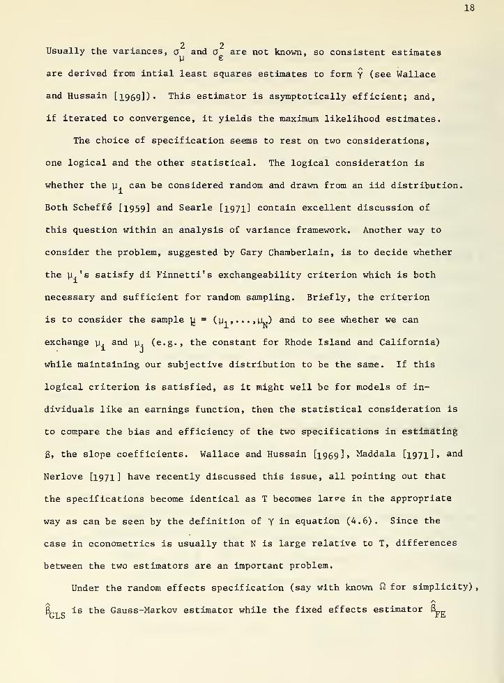
18

2 2Usually the variances, a and a are not known, so consistent estimatesy £

are derived from intial least squares estimates to form y (see Wallace

and Hussain [l969D« This estimator is asymptotically efficient; and,

if iterated to convergence, it yields the maximum likelihood estimates.

The choice of specification seems to rest on two considerations,

one logical and the other statistical. The logical consideration is

whether the y can be considered random and drawn from an iid distribution.

Both Scheffe [1959] and Searle [1971] contain excellent discussion of

this question within an analysis of variance framework. Another way to

consider the problem, suggested by Gary Chamberlain, is to decide whether

the y.'s satisfy di Finnetti's exchangeability criterion which is both

necessary and sufficient for random sampling. Briefly, the criterion

is to consider the sample y = (y..,...,y^) and to see whether we can

exchange y. and y. (e.g., the constant for Rhode Island and California)

while maintaining our subjective distribution to be the same. If this

logical criterion is satisfied, as it might well be for models of in-

dividuals like an earnings function, then the statistical consideration is

to compare the bias and efficiency of the two specifications in estimating

3, the slope coefficients. Wallace and Hussain [1969], Maddala [1971], and

Nerlove tl97l] have recently discussed this issue, all pointing out that

the specifications become identical as T becomes lar^e in the appropriate

way as can be seen by the definition of y in equation (4.6). Since the

case in econometrics is usually that N is large relative to T, differences

between the two estimators are an important problem.

Under the random effects specification (say with known £2 for simplicity)

,

(L T „ is the Gauss-Markov estimator while the fixed effects estimator &GLS tt

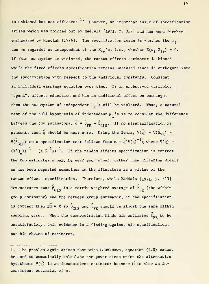
19

is unbiased but not efficient. * However, an important issue of specification

arises which was pointed out by Maddala [1971, p. 357] and has been further

emphasized by Mundlak [1976]. The specification issue is whether the y.

can be regarded as independent of the X. 's, i.e., whether E(u. |x. ) = 0.

If this assumption is violated, the random effects estimator is biased

while the fixed effects specification remains unbiased since it orthogonalizes

the specification with respect to the individual constants. Consider

an individual earnings equation over time. If an unobserved variable,

"spunk", affects education and has an additional effect on earnings,

then the assumption of independent y. 's will be violated. Thus, a natural

test of the null hypothesis of independent y . 's is to consider the difference

/v /v

between the two estimators, q = B - & . If no misspecification isr E CjLS

present, then q should be near zero. Using the lemma, V(q) = V(& ) -iE

V($ ) so a specification test follows from m = q'V(q) q where V(q) =VjLib

(X'Q X) - (X'fl X) . If the random effects specification is correct

the two estimates should be near each other, rather than differing widely

as has been reported sometimes in the literature as a virtue of the

random effects specification. Therefore, while Maddala [1971, p. 343]

demonstrates that 3„ T „ is a matrix weighted average of $ (the within

group estimator) and the between group estimator, if the specification

/\ v\ /\

is correct then Eq = so (3 and $_,_ should be almost the same withinuLo rE

sampling error. When the econometrician finds his estimates & to be

unsatisfactory, this evidence is a finding against his specification,

not his choice of estimator.

1. The problem again arises that with fi unknown, equation (2.8) cannot

be used to numerically calculate the power since under the alternative

hypothesis V(q) is an inconsistent estimator because Q is also an in-

consistent estimator of 0,.

20

The equivalent test in the regression format is to test a = from

doing least squares on

(4.7) y = X(3 + xa + v.

where y and X are the Y transformed random effects variables while X

are the deviations from means variables from the fixed effects specification.

The tests can be shown to be equivalent using the methods of the previous

two sections and the fact that Q y = Q y. This test is easy to perform

since X and X differ only in the choice of Y from equation (4.6) while

X has Y = 1.

The regression specification of equation (4.7) again makes power

considerations evident. The noncentrality parameter of the F-test is

proportional to the correlation of X and a which is the null hypothesis

being tested. If Y is near unity, then the two estimators will give

similar results and q will be near zero. The test of a from equation

(4.7) will depend on q and also on how close X and X and X are. If

they are quite different, V(q) will be small and then ot will be precisely

estimated. When they are similar, the specification test will not have

much power, but this case is not so important since the two estimates

of 6 will also be similar.

It will often be the case in econometrics that Y will not be near

unity. In many applications 0~ is small relative to O • and the problemU c,

sometimes arises that when o~ is estimated from the data it turns out

to be negative. For a panel followed over time the X. are often nearly

constant or trend smoothly with time so that much of the interindividual

variation disappears into the individual constants when the fixed effects

21

estimator is used. However, it seems preferable to have unbiased estimates

of the remaining slope coefficients by using a fixed effects specification

and then attempt to sort out the effects of education, "spunk", and their

interaction through a parametrization of the individual constants. The

misspecification test from equation (4.7) thus seems a desirable test of

the two different specifications.

In this section a test of the implicit assumption behind the random

effects specification has been considered. This test should follow the

logical specification of whether the y. are truly random. Thus, the

situation is very similar to simultaneous equation estimation which

follows the logical question of identification. In the next section,

the specification of simultaneous equation systems is considered, and

a test is developed for correct system specification.

22

5. Specification of Simultaneous Equation Systems

Most estimation associated with simultaneous equation models has

used single equation, limited information estimators. Thus, two stage

least squares (2SLS) is by far the most widely used estimator. If a

simultaneous equation system is estimated equation by equation, no check

on the "internal consistency" of the entire specification is made. An

important potential source of information on misspecif ication is thus

neglected. This neglect is not total; one class of tests compares estimates

of the unrestricted reduced form model with the estimates of the structural

model as a test of the overidentifying restrictions. * Unfortunately,

this type of test has not been been widely used. Perhaps the reason has

been the inconvenience of calculating the likelihood value or the nonlinear

expansions which are required to perform the statistical comparison.

In this section a test of system specification is proposed within a more

simple framework. The test rests on a comparison of 2SLS to 3SLS estimates.

Under the null hypothesis of correct specification, 3SLS is efficient but

yields inconsistent estimates of all equations if any equation is mis-

specified. 2SLS is not as efficient as 3SLS, but only the incorrectly

specified equation is inconsistently estimated if misspecification is

present in the system.

Consider the standard linear simultaneous equation model

(5.1) yb + zr = U

1. Within the single equation context this test has been proposed by

Anderson and Rubin [1949], Basmann [1957], and Hood and Koopmans [1953].Within the full information context the likelihood ratio (LR) test has

been used. Recently, Byron [1972, 1974] has simplified this test byadvocating use of the Lagrange multiplier test or the Wald test both of

which are asymptotically equivalent to the LR test under the null hypothesis.

For further details see Silvey [l970> Ch. 7],

23

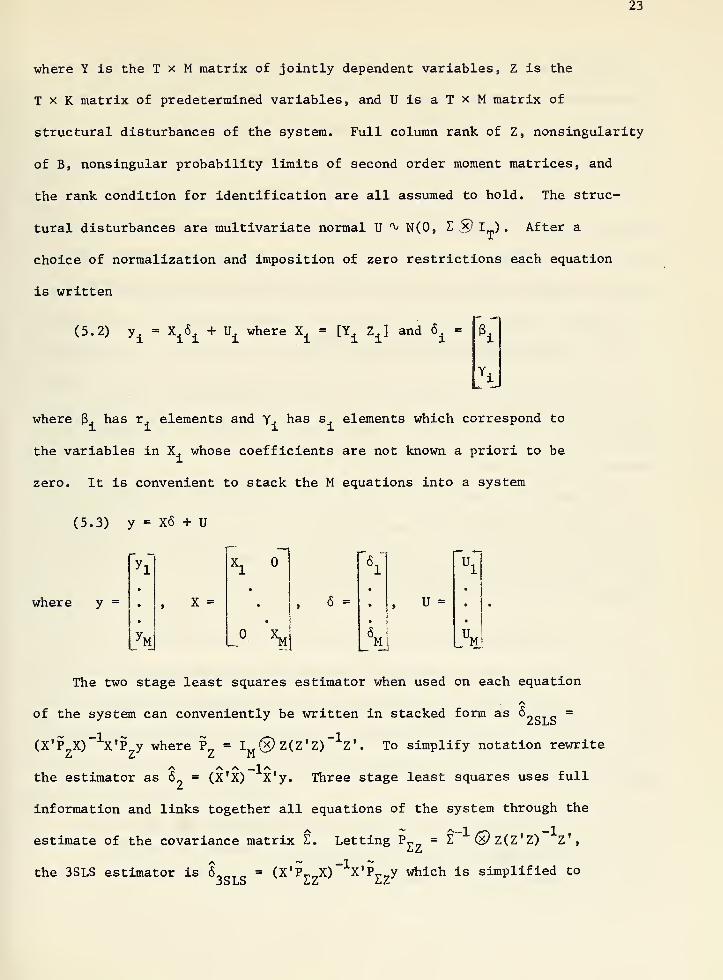
where Y is the T x M matrix of jointly dependent variables, Z is the

T x K matrix of predetermined variables, and U is a T x M matrix of

structural disturbances of the system. Full column rank of Z, nonsingularity

of B, nonsingular probability limits of second order moment matrices, and

the rank condition for identification are all assumed to hold. The struc-

tural disturbances are multivariate normal U ^ N(0, E %) I ) . After a

choice of normalization and imposition of zero restrictions each equation

is written

(5.2) y. = X.6. + U. where X. = [Y. Z .] and 6. =

J ± ii i lii i3,

Y,

where 3. has r. elements and Y.. has s. elements which correspond tox i i i

the variables in X, whose coefficients are not known a priori to be

zero. It is convenient to stack the M equations into a system

(5.3) y = X6 + U

where y =

~

yl~

Xl \ \

•

• , X =•

, 6 =• , H- •

•

yM

•

lj» I- Al

The two stage least squares estimator when used on each equation

of the system can conveniently be written in stacked form as 6„ =

(X'P X) X*P y where P = IM(x) Z(Z'Z) Z\ To simplify notation rewrite

the estimator as 6_ = (X'X) X'y* Three stage least squares uses full

information and links together all equations of the system through the

estimate of the covariance matrix £. Letting P^ = E~ (S)z(Z'Z)" Z',

the 3SLS estimator is 5 = (X'P^, X) X'P^ y which is simplified to

24

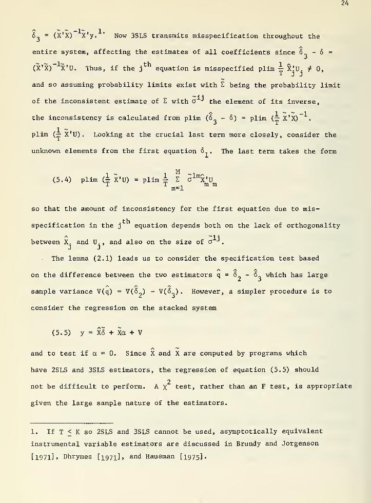
6„ = (X'X) X'y. " Now 3SLS transmits misspecification throughout the

entire system, affecting the estimates of all coefficients since 6 - 6 =

(X'X) X'U. Thus, if the j equation is misspecif ied plim ^ X!u. t 0,

and so assuming probability limits exist with E being the probability limit

of the inconsistent estimate of E with o -1 the element of its inverse,

the inconsistency is calculated from plim (6 - 6) = plim (—X'X)

plim (— X'U). Looking at the crucial last term more closely, consider the

unknown elements from the first equation 5 . The last term takes the form

M(5.4) plim (i X'U) = plim ± E a^X'U

T T . m mm=l

so that the amount of inconsistency for the first equation due to mis-

specification in the j equation depends both on the lack of orthogonality

~libetween X. and U., and also on the size of O .

3 J

The lemma (2.1) leads us to consider the specification test based

/\ /^

on the difference between the two estimators q = 6 - 6 which has large

/\ /\ /s

sample variance V(q) = V(6 ) - V(6 ) . However, a simpler procedure is to

consider the regression on the stacked system

(5.5) y = X6 + Xa + V

and to test if a = 0. Since X and X are computed by programs which

have 2SLS and 3SLS estimators, the regression of equation (5.5) should

2not be difficult to perform. A X test, rather than an F test, is appropriate

given the large sample nature of the estimators.

1. If T < K so 2SLS and 3SLS cannot be used, asymptotically equivalent

instrumental variable estimators are discussed in Brundy and Jorgenson

tl97l]» Dhrymes [1971], and Hausman [1975].

25

2The noncentrality parameter of the x distribution will be proportional

1 ~to plim — X'U. for any equation which is misspecif ied and also the magnitude

of the covariance elements o . If the inverse covariance elements are

large, then X and X will not be highly correlated so that the test will

be powerful for a given size of inconsistency. As the O -"'s go to zero,

then 3SLS approaches 2SLS and the test will have little power. Since

the misspecification represented by the alternative hypothesis is not

specific, the appropriate action to take in the case of rejection of

H„ is not clear. One only knows that misspecification is present somewhere

in the system. If one were confident that one or more equations are

correctly specified, then the specification of other equations could be

checked by using them, say one at a time, to form a 3SLS type estimator.

That is, if equation 1 is correct and equation 2 is to be tested, then

2SLS on equation 1 could be compared to 3SLS on equation 1 where O..

is set to zero for i £ j except for i = 1, j = 2 and vice-versa in the

3SLS estimator. Using this method the misspecification might be isolated;

but, unfortunately, the size of the test is too complicated to calculate

when done on a sequence of equations.

The simultaneous equations specification test is the last to be

presented although the same principle may be applied to further cases.

Before presenting two examples of the test, the issue of minimum mean

square estimators (MMSE) is discussed. These estimators might be thought

to be appropriate to use if the null hypothesis is rejected when the condi-

tion of unbiasedness is relaxed.

26

6. Pretesting and Minimum Mean Square Error Estimation

All the specification tests discussed so far have a single purpose:

to test whether the specification of the statistical model is correct.

The sample at hand is used for this purpose; and with respect to formal

received theory, that should be the end of the story. However, upon

deciding whether or not to reject Hn , the same data is often used to attempt

further inferences utilizing the estimator which the specification test

indicated is "correct". For example, the regression specification y = XB + £

may have an associated test of the hypothesis Hn : R3 = r (Theil's specifica-

tion theorem concerns a subvector of 3 being zero) . After using an F test

to determine whether to reject Hn , either the restricted or unrestricted

least squares estimator is used to provide estimates for further inference.

The properties of these so-called "pretest" estimators were first studied

in a classic paper by Bancroft [1944] who showed that both bias and loss

of efficiency may be introduced using such procedures. A long list of

papers on pretest estimators has followed which will not be reviewed

here. The point of this discussion is to mention the fact that only if

the restrictions are imposed a priori, presumably because they are known

to be true without any pretesting, do the classical statistical properties

hold.

Besides the problem of pretesting, the other issue common to specifica-

tion tests is minimum mean square error (MMSE) estimators. The mean

square error (MSE) of an estimator is the bias squared plus the variance.

The classical estimators of econometrics are all limited to unbiased

estimators which then minimize the variance under appropriate statistical

assumptions. In fact, one interpretation of the specification tests

proposed here is to determine if the models satisfy these statistical

27

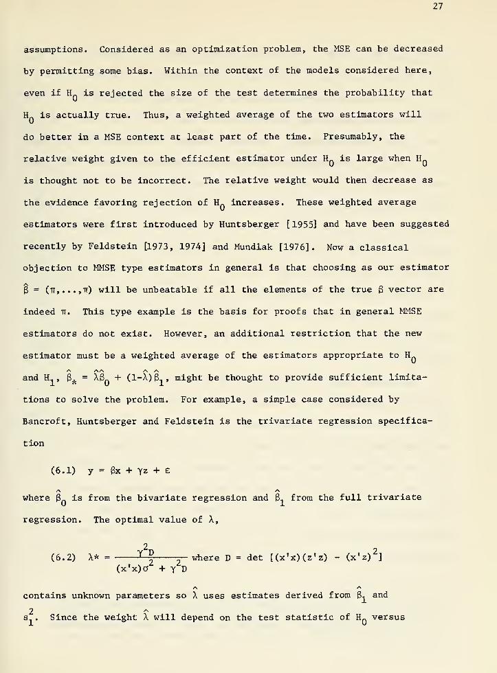
assumptions. Considered as an optimization problem, the MSE can be decreased

by permitting some bias. Within the context of the models considered here,

even if H_ is rejected the size of the test determines the probability that

Hn is actually true. Thus, a weighted average of the two estimators will

do better in a MSE context at least part of the time. Presumably, the

relative weight given to the efficient estimator under H„ is large when HQ

is thought not to be incorrect. The relative weight would then decrease as

the evidence favoring rejection of Hn

increases. These weighted average

estimators were first introduced by Huntsberger [ 1955] and have been suggested

recently by Feldstein [1973, 1974] and Mundlak [1976]. Now a classical

objection to MMSE type estimators in general is that choosing as our estimator

3 = (it it) will be unbeatable if all the elements of the true 3 vector are

indeed it. This type example is the basis for proofs that in general MMSE

estimators do not exist. However, an additional restriction that the new

estimator must be a weighted average of the estimators appropriate to H~

and H.. , 3* = A3,, + (1-A) 3, , might be thought to provide sufficient limita-

tions to solve the problem. For example, a simple case considered by

Bancroft, Huntsberger and Feldstein is the trivariate regression specifica-

tion

(6.1) y = 3x + yz + E

where 3n is from the bivariate regression and 3-, from the full trivariate

regression. The optimal value of A,

(6.2) X* = *-| _ where D = det [(x'x)(z'z) - (x'z)2

]

(x'x)a + YD

contains unknown parameters so A uses estimates derived from 3i and

2s . Since the weight A will depend on the test statistic of H~ versus

28

H1which is consistent, X will go to zero as the sample becomes large if

HQ

is not true. Thus, in large samples the estimate is consistent but

the MSE properties of interest will usually be finite sample properties

since for large samples the pretest estimator (X = or X = 1) will

lead to the correct estimator. For finite samples, even within the

restricted class of weighted average estimators no MMSE estimator will

exist in general. This result can be seen easily since X is a statistic

and for H being nearly true the weighted average estimator will not give

enough weight to 3ndue to the uncertainty of the true X. Statements

which attempt to give guidance about which estimator to use (i.e., a priori

choice of X) conditional on the researcher's "confidence" about the size

of unknown parameters or unknown test statistics seem an undesirable

form of "back-door Bayesianism" . The correct use of prior knowledge

is provided by Bayesian analysis which is superior to such "rules of thumb"

estimators.

The other rationale sometimes advocated in the use of such estimators

is that the researcher is not interested in certain of the parameters.

With unbiased estimators, Gauss-Markov or minimum variance estimation

assures us that c'B is the best estimator of c'3 for 3 minimum variance

and c an arbitrary vector. For certain choices of c within the MSE

framework, it is true that unbiased minimum variance estimators are no

longer uniformly best. But, neither will MMSE estimator be best in all

situations just as before. Furthermore, since other researchers are un-

likely to have the same c, the correct procedure is to report both 3~ and

1. It is interesting to note that for any unknown 3, the unbiased OLS

estimator may be uniformly improved upon for any quadratic loss function

if the unknown t statistic for y is known to be bounded. While Feldstein

[1973] advocates use of the t statistic as a rule of thumb, his estimator

is not the one which offers this uniform improvement. For details see

Perlman [1972 ].

29

3, along with their associated covariance matrices. Users of the research

can then decide if they are convinced by the tests conducted and apply

their own weights to form their favorite estimates. Reporting only the

weighted estimates is condensing the original data too far since the re-

sults depend on either the original researcher's confidence about A or

choice of c which are unlikely to be shared by his readers.

30

7 . Empirical Examples

Comparing two alternative estimators as a means of constructing

misspecif ication tests has been applied to a number of situations in

the preceding sections. In this section two empirical examples are

presented. Both examples are new tests of misspecification and likely

to be of interest to the applied econometrician. The first example is

the time series - cross section specification test discussion in Section 4.

This type of data set is becoming increasingly common for econometric

studies such as individuals' earnings, education, and labor supply. How-

ever, added interest in this test comes from the fact that it also im-

plicitly tests much cross section analysis of similar specifications.

Cross section analysis can allow for no individual constant but must as-

sume, as does random effect analysis, that the right hand side variables

are orthogonal to the residual: If the random effect specification is

rejected serious doubt may be cast therefore on much similar cross section

analysis. The second empirical example is the simultaneous equations

specification test of Section 5. The famous Klein Model I is used as an

example since it has been thoroughly analyzed in the past and is a con-

venient example. Previous tests of the model have been tests mainly of the

overidentifying restrictions on the structural form. Here by comparing

2SLS and 3SLS estimates of the model, the correctness of the overall speci-

fication is tested.

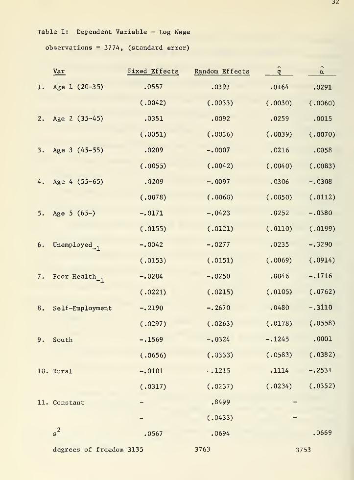
For the time series - cross section specification test a wage equation

is estimated for male high school graduates in the Michigan Income Dynamics

Study. ' The sample consists of 629 individuals for whom all six years

1. The specification used is based on research by Gordon [1976] who also

kindly helped me construct this example.

31

of observations are present . A wage equation has been chosen due to its

importance in "human capital" analysis. The specification used follows

from equation (4.1). The right hand side variables include a piecewise

linear representation of age, the presence of unemployment or poor health

in the previous year, and dummy variables for self-employment, living

/*.

in the South or in a rural area. The fixed effects estimates, 3t™» arer E

calculated from equation (4.3). They include an individual constant

for each person and are unbiased under both the null hypothesis of no

misspecification and the alternative hypothesis. The random effects

estimates, 3GT c» are calculated from equations (4.4)-(4.6). The estimate

of y from equation (4.6) is .72736 which follows from least squares esti-

~2 ~2mates of the individual variance a = .12594 and the residual variance a =

y e

.06068. Under the null hypothesis the GLS estimate is asymptotically

efficient, but under the alternative hypothesis it is inconsistent.

The specification test consists of seeing how large the difference in

estimates is, q = g_„ - B~ T , in relation to its variance V(q) = V(6„„) -rb uLo ft

V($ ) which follows from Lemma (2.1). In comparing the estimates in

column 1 and column 2 of Table 1 it is apparent that substantial differ-

ences are present in the two sets of estimates relative to their standard

errors which are presented in column 3. The effects of unemployment,

self-employment, and geographical location differ widely in the two models.

For instance, the effect of unemployment in the previous year is seen

1. Note that the elements of q and its standard errors are simply cal-

culated given the estimates of g and 3~TC, and their standard errorsr E (jLS ry

making sure to adjust to use the fixed effects estimate of a . The

main computational burden involves forming and inverting V(q)

.

il

Table I: Dependent Variable - Log Wage

observations = 3774, (standard error)

Var

1. Age 1 (20-35)

2. Age 2 (35-45)

3. Age 3 (45-55)

4. Age 4 (55-65)

5. Age 5 (65-)

6. Unemployed,

7. Poor Health,

8. Self-Employment

9. South

10. Rural

11. Constant

2s

degrees of freedom 3135

Fixed Effects Random Effects

.0393

q a

.0557 .0164 .0291

(.0042) (.0033) (.0030) (.0060)

.0351 .0092 .0259 .0015

(.0051) (.0036) (.0039) (.0070)

.0209 -.0007 .0216 .0058

(.0055) (.0042) (.0040) (.0083)

.0209 -.0097 .0306 -.0308

(.0078) (.0060) (.0050) (.0112)

-.0171 -.0423 .0252 -.0380

(.0155) (.0121) (.0110) (.0199)

-.0042 -.0277 .0235 -.3290

(.0153) (.0151) (.0069) (.0914)

-.0204 -.0250 .0046 -.1716

(.0221) (.0215) (.0105) (.0762)

-.2190 -.2670 .0480 -.3il0

(.0297) (.0263) (.0178) (.0558)

-.1569 -.0324 -.1245 .0001

(.0656) (.0333) (.0583) (.0382)

-.0101 -.1215 .1114 -.2531

(.0317) (.0237) (.0234) (.0352)

- .8499

- (.0433)

.0567 .0694 .0669

3135 3763 3753

33

to be much less important in effecting the wage in the fixed effects

specification. Thus, unemployment has a more limited and transitory

effect once permanent individual differences are accounted for. The test

of misspecification follows from Lemma 2.1 is

(7.1) m =q' V

ff"^

= 12.99.

Since m is distributed approximately as F(10, °°) which has a critical

value of 2.32 at the 1% level, very strong evidence of misspecification

in the random effects model is present. The right hand side variables

X. are not orthogonal to the individual constant u. so that the null

hypothesis is decisively rejected. Considerable doubt about much previous

cross section work on wage equations arises from this example.

The reason for this doubt about previous cross section estimation

is that ordinary least squares on a cross section of one year will have

/\

the same expectation as $ , the random effects estimate, on the timeCjLo

series - cross section data. For example, cross section estimates of

the wage equation have no individual constants and make Assumption (1.1. a.)

that the residual is uncorrelated with the right hand side variables.

However, this example demonstrates that in the Michigan Survey important

individual effects are present which are not uncorrelated with the right

hand variables. Since the random effects estimates seem significantly

biased with high probability, then previous cross section estimates

of wage and earnings equations may also be significantly biased. This

problem can only be resolved within a time series - cross section frame-

1. Direct estimates of the effect of education are not possible in thefixed effects approach, but the example shows that models which usethis specification may well be misspecif ied.

34

work using a specification which allows testing of an important maintained

hypothesis of much cross section estimation in econometrics.

An equivalent formulation of the specification test is provided

by the regression framework of equation (A. 7). Instead of having to

manipulate 10 x 10 matrices, y is regressed on both X and X. The test

of the null hypothesis is then whether a = 0. As is apparent from column 4

of Table 1 many of the elements of a are well over twice their standard

error so that misspecif ication is clearly present. The misspecif ication

2test follows easily from comparing s , the estimated variance, from the

2random effects specification to s from the augmented specification

/-, on .06938 - .06689 3754 ., __.(7,2) m ^6689 JQ-

=13.974.

Again m well exceeds the approximate critical F value of 2.32. Since this

form of the test is so easy to implement when using a random effects speci-

fication as only one additional weighted least squares regression is re-

quired, hopefully applied econometricians will find it a useful device for

testing specification.

The second empirical example is a test of Klein Model I. This seminal

model has 3 equations for consumption, investment, and labor and is estimated

on annual data from 1920-1941. It is known that the hypothesis of the

overidentifying restrictions is rejected for the model. Thus, the mis-

specification test may not have great power since under just identification

the 2SLS and 3SLS estimates are identical. Still, the test may allow

us to derive further evidence about the model. Here 2SLS estimates will

be consistent for all but the misspecified equation under the alternative

35

specification while the 3SLS estimates for all equations will be incon-

sistent. Another determinant of the power of the test is the covariance

matrix E since if it is diagonal 2SLS and 3SLS estimates are again identical.

The 2SLS estimate E, however, shows substantial covariance between the

equations.

1.044

.4378 1.383

-.3852 .1926 .4764

(7 ' 3>

Z2SLS

!

When comparing the 2SLS and 3SLS estimates in Table 2, the estimated

coefficients are quite similar relative to their standard errors as seen

in column 3. Thus q = 6„ - 6 does not present much evidence of misspeci-

2 /> /v

fication. Forming a x test from q and its estimated variance V(q) =

/\ /\

V(6 ) - V(<5„) leads to a value

(7.4) m = q*V(q)-1

q = 12.71

2Since m is distributed as Xi o » the test presents little evidence in favor

of misspecif ication since the expected value of m under the null hypothesis

is 12. Whenever the null hypothesis is not rejected, the power of the test

is of considerable interest. Here power considerations are evident in

using the stacked regression formulation of equation (5.5) to check the

estimates of relative to their standard errors. With this alternative

2approach m is calculated to be 5.78 which is distributed as x7

so no evi-

dence of misspecification is present. " However, by considering the stand-

ard errors the test is seen not to have great power since a from equation

1. In the combined regression framework of equation (5.5) constantsare eliminated from X and each right hand side variable appears only

once. Therefore, in the stacked framework, the operating characteristicsof the alternative tests are not identical.

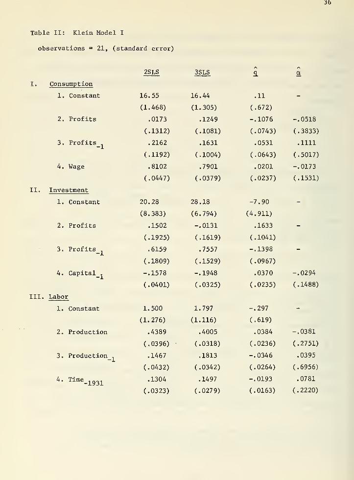
Table II: Klein Model I

observations = 21, (standard error)

36

2SLS 3SLS a

I. Consumption

1. Constant 16.55 16.44 .11 -

(1.468) (1.305) (.672)

2. Profits .0173 .1249 -.1076 -.0518

(.1312) (.1081) (.0743) (.3833)

3. Profits .2162 .1631 .0531 .1111

(.1192) (.1004) (.0643) (.5017)

4. Wage .8102 .7901 .0201 -.0173

(.0447) (.0379) (.0237) (.1531)

II. Investment

1. Constant 20.28 28.18 -7.90 -

(8.383) (6.794) (4.911)

2. Profits .1502 -.0131 .1633 -

(.1925) (.1619) (.1041)

3. Profits .6159 .7557 -.1398 -

(.1809) (.1529) (.0967)

4. Capital1

-.1578 -.1948 .0370 -.0294

(.0401) (.0325) (.0235) (.1488)

III. Labor

1. Constant 1.500 1.797 -.297 -

(1.276) (1.116) (.619)

2. Production .4389 .4005 .0384 -.0381

(.0396) (.0318) (.0236) (.2751)

3. Production1

.1467 .1813 -.0346 .0395

(.0432) (.0342) (.0264) (.6956)

4. Time_1931

.1304

(.0323)

.1497

(.0279)

-.0193

(.0163)

.0781

(.2220)

37

(5.5) is not at all precisely estimated. Some of the elements of a are

large relative to their estimated value in 6 from equation (5.5), e.g.

profits, but the estimated standard errors are so large that the test

cannot determine if this result follows from misspecif ication or from

statistical fluctuation.

The two empirical examples presented in this section illustrate

use of the misspecif ication test. The first example rejects an applica-

tion of the random effects specification and thereby casts doubt on much

cross section work in this area. I feel that this finding is probably

quite general, and that the random effects model is not well suited to

most econometric applications. The two requirements of exchangeability

and orthogonality are not likely to be met in our applied problems.

Certainly, these specifications should be tested for correct specification.

The second example demonstrates how power considerations are evident when

the null hypothesis is not rejected. Also, it demonstrates the potential

usefulness of full information estimators in determining the correctness of

specification in simultaneous equation models.

38

8. Conclusion

By using the result that under the null hypothesis of no misspecif ica-

tion, an efficient estimator must be uncorrelated with its difference

from an unbiased but inefficient estimator, specification tests are de-

vised for a number of important model specifications in econometrics.

New tests for the cross section - time series model and for the simul-

taneous equation model are presented. The possibility of combining the

two estimators into a MMSE estimator is discussed, and it is pointed out

that the type of knowledge needed for such estimators is better used within

a proper Bayesian framework. Lastly, two empirical examples are provided.

The first example provides strong evidence against a specification commonly

used in time series - cross section work and also provides evidence

questioning much cross section analysis currently being done on individual

data in econometrics.

39

References

Anderson, T.W. and Rubin, H., "Estimation of the Parameters of a Single

Stochastic Equation in a Complete System of Stochastic Equations",

Annals of Mathematical Statistics , 20, 1949, pp. 46-63

Bancroft, T.A. , "On Biases in Estimation due to the Use of Preliminary

Tests of Significance", Annals of Mathematical Statistics , 15, 1944,

pp. 190-204

Basmann, R.L., "A Generalized Classical Method of Linear Estimation

of Coefficients in a Structural Equation", Econometrica , 25, 1957,

pp. 77-83

Brundy, J. and Jorgenson, D.W., "Efficient Estimation of Simultaneous

Equation Systems by Instrumental Variables, Review of Economics

and Statistics , 53, 1971, pp. 207-224

Byron, R.P., "Testing for Misspecif ication in Econometric Systems Using

Full Information", International Economic Review , 13, 1972, pp. 745-756

, "Testing Structural Specification Using the Unrestricted

Reduced Form", Econometrica , 42, 1974, pp. 869-883

Dhrymes, P.J., "A Simplified Structural Estimator for Large-Scale Econometric

Models", Australian Journal of Statistics , 13, 1971, pp. 168-175

Feldstein, M., "Multicollinearity and the Mean Square Error of Alternative

Estimators", Econometrica , 41, 1973, pp. 337-346

, "Errors in Variables: A Consistent Estimator

with Smaller Mean Square Error in Finite Samples", Journal of American

Statistical Association , 69, 1974, pp. 990-996

4U

Gordon, R., "Essays on the Causes and Equitable Treatment of Differences

in Earnings and Ability", MIT PhD Thesis, June 1976

Griliches, Z„, "Specification Bias in Estimates of Production Functions",

Journal of Farm Economics , 39, 1957, pp. 8-20

Hausman, J., "An Instrumental Variable Approach to Full-Information

Estimators for Linear and Certain Nonlinear Econometric Models",

Econometrica , 43, 1975, pp. 727-738

Huntsberger, D.V., "A Generalization of a Preliminary Test Procedure

for Pooling Data, Annals of Mathematical Statistics , 26, 1955,

pp. 734-743

Koopmans, T.C. and Hood, W. , "The Estimation of Simultaneous Economic

Relationships", in Hood and Koopmans (eds.), Studies in Econometric

Method , New Haven, 1953, pp. 113-199

Liviatan, N., "Tests of the Permanent Income Hypothesis Based on a Re-

interview Savings Study", in Measurement in Economics , C. Christ,

ed., Stanford, 1963, pp. 29-59

Maddala, G.S., "The Use of Variance Components Models in Pooling Cross

Section and Time Series Data", Econometrica , 39, 1971, pp. 341-358

Mundlak, Y., "On the Pooling of Time Series and Cross Section Data",

1976, mimeo.

Nerlove, M. , "A Note on Error Component Models", Econometrica , 39, 1971,

pp. 383-396

41

Perlman, M.D. , "Reduced Mean Square Error Estimation for Several Parameters",

Sankhya , B, 34, 1972, pp. 89-93

Rao, C.R. , Linear Statistical Inference , New York, 1973

Sargan, J.D„, "The Estimation of Economic Relationships Using Instrumental

Variables", Econometrica , 26, 1958, pp. 393-415

Scheffe, H., Analysis of Variance , New York, 1959

Searle, P., Linear Models , New York, 1971

Silvey, S.D., Statistical Inference , London, 1970

Theil, H., "Specification Errors and the Estimation of Economic Relation-

ships", Review of the International Statistical Institute , 25,

1957,. pp. 41-51

Wallace, T.D. and Hussain, A., "The Use of Error Components Models in

Combining Cross Section with Time Series Data", Econometrica ,

37, 1969, pp. 57-72

Wu, D., "Alternative Tests of Independence Between Stochastic Regressors

and Disturbances", Econometrica, 41, 1973, pp. 733-750