species distribution modeling - central web server 2...

Species Distribution Modeling

Day 1: GLMs and GAMs

Outline 1.  Species Distribution Models (SDMs) 2.  Generalized Linear Models (GLMs) 3.  Generalized Additive Models (GAMs)

What is a Species Distribution Model (SDM)?

  Predicts where a species probably is and probably isn’t

  Predict the probability of presence (or tries to)

  Input data   Presence/Absence (for probability of presences)

OR   Presence only (for relative probability of presence)

+   Environmental covariates at sample sites (to fit a model)

OR   Environmental covariates on a map (to predict)

What is a Species Distribution Model (SDM)?

Why SDMs?   Predictive Models:

  Predict species presence at unsampled locations   Predict occurrence under new conditions, like under climate

change or invasion

  Explanatory Models:   Determines what environmental covariates that drive species

abundance   Determine shape of response to environmental covariates

  Make pretty maps

What is an SDM?   Correlative   Non-mechanistic   Static in time   Potential distribution, not realized distribution

Some subtleties   Presence/Absence Data vs. Presence Data   Absences vs. Pseudo absences   Relative numbers of presences and absences   What does the probability of presence mean?

  If p=0.6 given the environmental covariates X that means 60% of the sites exactly like X have the species

  Thresholding   Spatial mismatch of occurrence and environmental data   Physioloigical importance of commonly available climatic

variables   Projecting outside the range of observed independent

variables (e.g. no-analogue climates)

Today’s Modeling Methods

  Generalized Linear Models (GLMs)

  Generalized Additive Models (GAMs)

€

logit(pi) = b0 + b1x1i + b2x2i ++ε i

€

logit(pi) = b0 + f1(x1i) + b2x2i ++ε i

€

yi ~ Binomial(pi,ni)Logistic regression

yi are summaries of ni Bernoulli trials

Smoothing spline

Logistic regression in ecology   For anything where the response is binary   Population growth – logistic function includes carrying

capacity   Presence/absence – species distributions   Survival – demographic models   Germination

Generalized Linear Models   What’s generalized about them?

  In linear regression we assume the residuals are normally distributed with constant variance. GLMs generalize this assumption by allowing for other types of error distributions

  We use logistic regression for SDMs because we have binary data   Binary data is binomially distributed and residuals have

NONconstant variance p(1-p)   Others nonconstant error distributions are possible

  Poisson for count data has residual variance equal to the mean value of the response (larger # counts => larger variance in observation)

€


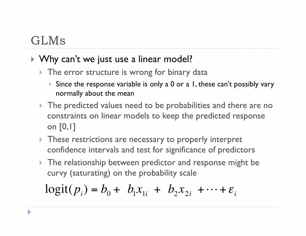
GLMs   Why can’t we just use a linear model?

  The error structure is wrong for binary data   Since the response variable is only a 0 or a 1, these can’t possibly vary

normally about the mean

  The predicted values need to be probabilities and there are no constraints on linear models to keep the predicted response on [0,1]

  These restrictions are necessary to properly interpret confidence intervals and test for significance of predictors

  The relationship between predictor and response might be curvy (saturating) on the probability scale

€


What does logistic regression model?   We provide 1’s and 0’s as response variables and we want

p, the probability of a 1 (i.e. observing the species)   For logistic regression we transform the linear predictor

using a link function   Link functions transform the expectation value to the same

interval that the response is on   Link functions

  Poisson - Log   Binomial – Logit, Probit   Gaussian- Uniform

€


What does logistic regression model?   Logistic regression uses the log of the odds ratio   Odds ratio = P(presence)/P(absence) = p/(1-p)

  Why use an odds ratio?   For a finite number (N) of categorical outcomes there are are

N-1 independent parameters to estimate. Modeling this ratio also ensures that P(presence) + P(absence) =1.

  The response variable is log( p/(1-p) ) = logit (p)

€


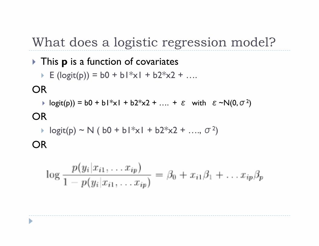
What does a logistic regression model?   This p is a function of covariates

  E (logit(p)) = b0 + b1*x1 + b2*x2 + ….

OR   logit(p)) = b0 + b1*x1 + b2*x2 + …. + ε with ε~N(0,σ2)

OR   logit(p) ~ N ( b0 + b1*x1 + b2*x2 + …., σ2)

OR

Interpreting GLMs   We interpret GLMs by looking at the values coefficients

associated with each predictor   Standardize predictors so coefficients comparable   A unit change in predictor xij results in a change of bj in

the response pi on the logit scale

  You must invert the logit transform to understand how changes in coefficients change on the probability scale

  Trick: divide a coefficient fit on the logit scale by 4 to get the maximum change in pi on the probability scale

€


Evaluating GLMs   How good is the fit, and are predictors significant?   How do we compare GLMs?

  In linear regression we ask about the Residual Sum of Squares (RSS)   e.g. we ask whether including an additional predictor reduces the RSS

by more than a we would expecet by chance

  In GLMs we ask the same questions about changes in the deviance

  Deviance   -2 * log ( likelihood )   See example in exercises

Evaluating GLMs   How do we use a deviance?

  The deviance is distributed as a chi-squared distribution with number of degrees of freedom equal to the number of data points minus the number of fitted parameters

  Given a deviance statistic, we compare it to the percentiles of the right chi-squared distribution

Statistical significance   How does one assess the statistical significance of something?

  You need a null hypothesis and a hypothesis to test it against   Model 1 is good enough (Null) vs. Model 2 is better (H1)

  You need a statistic that summarizes quantity you’re interested in   Deviance summarizes the difference in fit between the models

  You need to know how this statistic is distributed   Chi-squared with the right degrees of freedom

  If the statistic falls in the tail of the distribution, we can reject the null hypothesis.   If model 2 reduces the deviance * a lot * then it’s probably better

  P-values give the percentile of the distribution where the statistic falls   e.g. p gives the proportion of time we’d be wrong by taking model 2

  Fortunately statisticians love to figure out what the right statistic and its associated statistical distribution for a particular model so we just have to read their books sometimes

Exercise 1 - GLMs 1. Download the exercises here under Day 1:

http://web2.uconn.edu/cyberinfra/module3/outline.html

2. Get crackin’

3. In 45 minutes or so we’ll reconvene and discuss GAMs

Generalized Additive Models (GAMs)   Can be used wherever you’d normally use linear or

generalized linear models   More flexible than LM or GLM because very wiggly

response curves allowed

Generalized Additive Models (GAMs)   Instead of y ~ Σ xj βj we use y ~ Σf( xj) where f(xj) is

some wiggly function of the xj estimated from scatterplots

  Smoothing functions include: smoothing splines, locally weighted regression, kernel smoothers, or running mean/median smoothers but this choice seems relatively unimportant for our applications

  ‘Additive’ because no interaction terms

GAMs

Linear model vs. Cubic spline

Which line seems like a better fit?

Which has more assumptions?

GAMs

How wiggly is too wiggly?

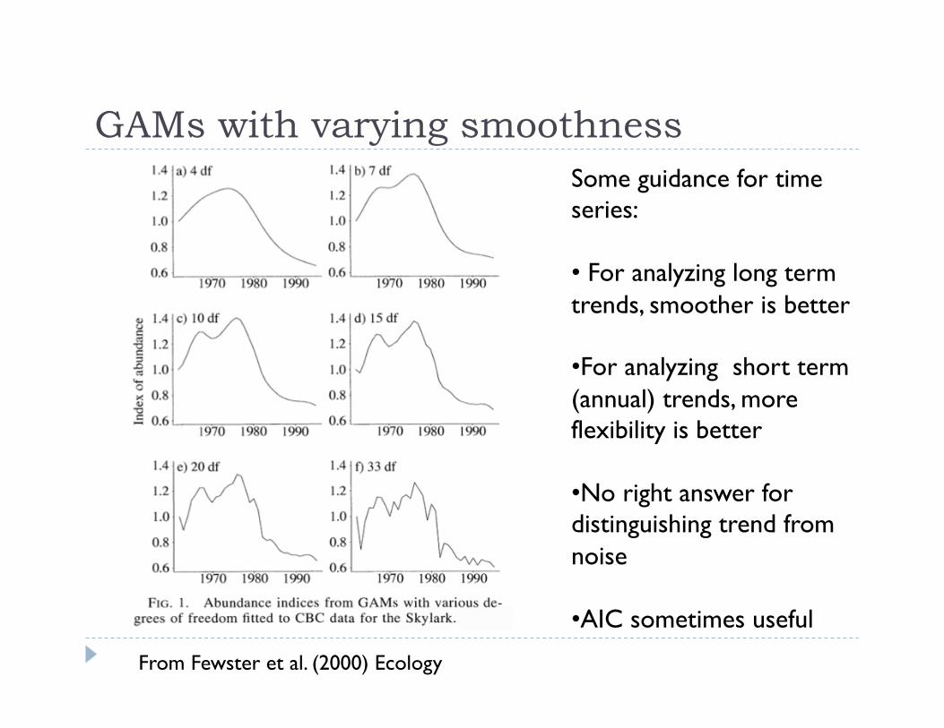
GAMs with varying smoothness Some guidance for time series:

•  For analyzing long term trends, smoother is better

• For analyzing short term (annual) trends, more flexibility is better

• No right answer for distinguishing trend from noise

• AIC sometimes useful

From Fewster et al. (2000) Ecology

GAMs – Bad example

This can be a bad idea sometime– what do you think?

GAMs – Is this one ok?

Time effects from single species CBC data. From Fewster et al. (2000) Ecology

GAMs in ecology

  Wiggly functions   Ecological theory suggests that ecological responses

should be unimodal, and not linear, hence GAMs   Presence/absence – species distributions   Physiological response to environment   Average community trait values along gradients   Modeling extremes   Temporal trends   List of GAM papers in ecology:

http://www.mendeley.com/research-papers/tag/generalized+additive+model/

GAMs – Good idea?   Pros:

  Some think this a very ‘pure’ approach to modeling because the data does all the talking

  Probably ok for explanatory models   Allows for complex response curves (e.g. bimodality)   Seems ok (to me) when you think there are other important

predictors omitted   Cons:

  Some people think this is ridiculous over fitting   A priori specification of amount of smoothness   Bad for interaction terms   Probably bad for predictions

Smoothers   Many types of scatterplot smoothers   Splines are piecewise polynomials that are popular for

their simplicity   Match 2 polynomials (e.g. two cubics) at a ‘knot’ and make

sure the derivatives are continuous   Running averages are also nice

How to make a GAM   Most smoothers making polynomials that fit subsets of

the data and splice them together–   include linear coefficient for each power of x   A cubic spline for y(x) is

y(x) = b0 + b1*x + b2*x2 + b3*x3

  Most algorithms fit these sort of cubic functions locally   Can choose which predictors you want linear functions

for and which you want smoothers for   Use AIC to choose which models are best since this

penalizes for the number of parameters   AIC doesn’t require nested models like analyses of deviance so

more flexible model comparison

Exercise 2 - GAMs 1. Continue with the exercises

2. Start on homework

3. Email me homework before next class

species distribution modeling - central web server 2...

Documents