J. Broida UCSD Fall 2009

Phys 130B QM II

Supplementary Notes on

Special Relativity and Maxwell’s Equations

1 The Lorentz Transformation

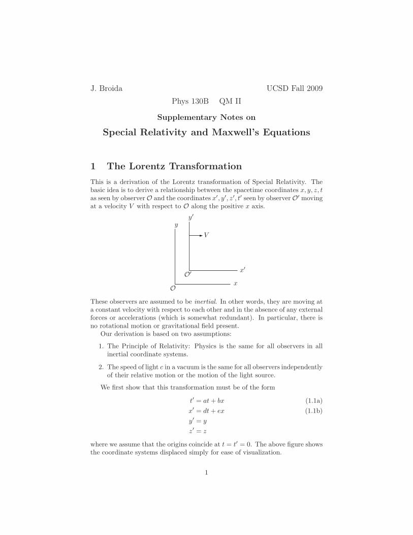
This is a derivation of the Lorentz transformation of Special Relativity. Thebasic idea is to derive a relationship between the spacetime coordinates x, y, z, tas seen by observer O and the coordinates x′, y′, z′, t′ seen by observer O′ movingat a velocity V with respect to O along the positive x axis.

x

y

x′

y′

O

O′

V

These observers are assumed to be inertial. In other words, they are moving ata constant velocity with respect to each other and in the absence of any externalforces or accelerations (which is somewhat redundant). In particular, there isno rotational motion or gravitational field present.

Our derivation is based on two assumptions:

1. The Principle of Relativity: Physics is the same for all observers in allinertial coordinate systems.

2. The speed of light c in a vacuum is the same for all observers independentlyof their relative motion or the motion of the light source.

We first show that this transformation must be of the form

t′ = at + bx (1.1a)

x′ = dt + ex (1.1b)

y′ = y

z′ = z

where we assume that the origins coincide at t = t′ = 0. The above figure showsthe coordinate systems displaced simply for ease of visualization.

1

The first thing to note is that the y and z coordinates are the same for bothobservers. (This is only true in this case because the relative motion is alongthe x axis only. If the motion were in an arbitrary direction, then each spatialcoordinate of O′ would depend on all of the spatial coordinates of O. However,this is the case that is used in almost all situations, at least at an elementarylevel.) To see that this is necessary, suppose there is a yardstick at the origin ofeach coordinate system aligned along each of the y- and y′-axes, and supposethere is a paintbrush at the end of each yardstick pointed towards the other.If O′’s yardstick along the y′-axis gets shorter as seen by O, then when theorigins pass each other O’s yardstick will get paint on it. But by the Principleof Relativity, O′ should also see O’s yardstick get shorter and hence O′ wouldget paint on his yardstick. Since this clearly can’t happen, there can be nochange in a direction perpendicular to the direction of motion.

The next thing to notice is that the transformation equations are linear.This is a result of space being homogeneous. To put this very loosely, “thingshere are the same as things there.” For example, if there is a yardstick lyingalong the x axis between x = 1 and x = 2, then the length of this yardstickas seen by O′ should be the same as another yardstick lying between x = 2and x = 3. But if there were a nonlinear dependence, say ∆x′ goes like ∆x2,then the first yardstick would have a length that goes like 22 − 12 = 3 while thesecond would have a length that goes like 32 − 22 = 5. Since this is also not theway the world works, equations (1.1) must be linear as shown. We now want tofigure out what the coefficients a, b, d and e must be.

First, let O look at the origin of O′ (i.e., x′ = 0). Since O′ is moving at aspeed V along the x-axis, the x coordinate corresponding to x′ = 0 is x = V t.Using this in (1.1b) yields x′ = 0 = dt + eV t or d = −eV . Similarly, O′ looksat O (i.e., x = 0) and it has the coordinate x′ = −V t′ with respect to O′ (sinceO moves in the negative x′ direction as seen by O′). Then from (1.1b) we have−V t′ = dt and from (1.1a) we have t′ = at, and hence t′ = −dt/V = at so that−aV = d = −eV and thus also a = e and d = −aV . Using these results inequations (1.1) now gives us

t′ = a

(

t +b

ax

)

(1.2a)

x′ = a(x − V t) (1.2b)

y′ = y

z′ = z.

Now let a photon move along the x-axis (and hence also along the x′-axis)and pass both origins when they coincide at t = t′ = 0. Then the x coordinateof the photon as seen by O is x = ct, and the x′ coordinate as seen by O′

is x′ = ct′. Note that the value of c is the same for both observers. This isassumption (2). Using these in equations (1.2) yields

t′ = a

(

t +b

act

)

= at

(

1 +bc

a

)

2

x′ = a(ct − V t) = cat

(

1 − V

c

)

so that

cat

(

1 − V

c

)

= x′ = ct′ = cat

(

1 +bc

a

)

and therefore −V/c = bc/a orb

a= −V

c2.

So now equations (1.2) become

t′ = a

(

t − V

c2x

)

(1.3a)

x′ = a(x − V t) (1.3b)

y′ = y

z′ = z.

We still need to determine a. To do this, we will again use the Principle ofRelativity. Let O look at a clock situated at O′. Then ∆x = V ∆t and from(1.3a), O and O′ will measure time intervals related by

∆t′ = a

(

∆t − V

c2∆x

)

= a

(

1 − V 2

c2

)

∆t.

Now let O′ look at a clock at O (so ∆x = 0). Then ∆x′ = −V ∆t′ so (1.3b)yields

−V ∆t′ = ∆x′ = a(0 − V ∆t) = −aV ∆t

and hence

∆t =1

a∆t′.

By the Principle of Relativity, the relative factors in the time measurementsmust be the same in both cases. In other words, O sees O′’s time related to hisby the factor a(1 − V 2/c2), and O′ sees O’s time related to his by the factor1/a. This means that

1

a= a

(

1 − V 2

c2

)

or

a =1

√

1 − V 2

c2

3

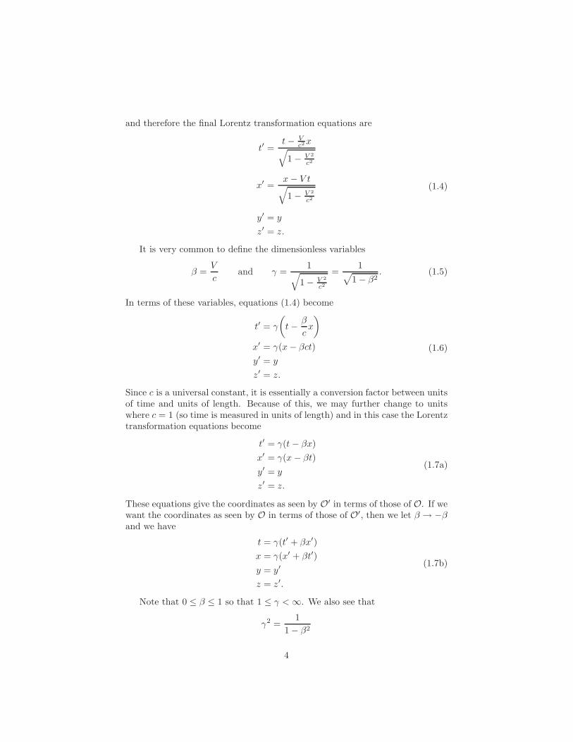
and therefore the final Lorentz transformation equations are

t′ =t − V

c2 x√

1 − V 2

c2

x′ =x − V t

√

1 − V 2

c2

y′ = y

z′ = z.

(1.4)

It is very common to define the dimensionless variables

β =V

cand γ =

1√

1 − V 2

c2

=1

√

1 − β2. (1.5)

In terms of these variables, equations (1.4) become

t′ = γ

(

t − β

cx

)

x′ = γ(x − βct)

y′ = y

z′ = z.

(1.6)

Since c is a universal constant, it is essentially a conversion factor between unitsof time and units of length. Because of this, we may further change to unitswhere c = 1 (so time is measured in units of length) and in this case the Lorentztransformation equations become

t′ = γ(t − βx)

x′ = γ(x − βt)

y′ = y

z′ = z.

(1.7a)

These equations give the coordinates as seen by O′ in terms of those of O. If wewant the coordinates as seen by O in terms of those of O′, then we let β → −βand we have

t = γ(t′ + βx′)

x = γ(x′ + βt′)

y = y′

z = z′.

(1.7b)

Note that 0 ≤ β ≤ 1 so that 1 ≤ γ < ∞. We also see that

γ2 =1

1 − β2

4

so thatγ2 − γ2β2 = 1.

Then recalling the hyperbolic trigonometric identities

cosh2 θ − sinh2 θ = 1

and1 − tanh2 θ = sech2 θ

we may define a parameter θ (sometimes called the rapidity) by

β = tanh θ

so thatγ = cosh θ

andγβ = sinh θ.

In terms of θ, equations (1.7a) become

t′ = (cosh θ)t − (sinh θ)x

x′ = −(sinh θ)t + (cosh θ)x

y′ = y

z′ = z

(1.8)

which looks very similar to a rotation in the xt-plane, except that now we havehyperbolic functions instead of the usual trigonometric ones. However, notethat both sinh terms have the same sign.

Next, let us consider motion as seen by both observers. In this case we writedisplacements in both space and time as

dt′ = γ(dt − βdx)

dx′ = γ(dx − βdt)

dy′ = dy

dz′ = dz.

Then the velocity v′x of a particle along the x′-axis as seen by O′ is

v′x =dx′

dt′=

dx − βdt

dt − βdx=

dx/dt − β

1 − β(dx/dt)=

vx − β

1 − βvx. (1.9a)

Alternatively, we may write

vx =dx

dt=

dx′ + βdt′

dt′ + βdx′=

dx′/dt′ + β

1 + β(dx′/dt′)=

v′x + β

1 + βv′x. (1.9b)

These last two equations are called the relativistic velocity addition law. Itshould be obvious that for motion along the x-axis we have v′y = vy and v′z = vz .

5

Be sure to understand what these equations mean. They relate the velocity ofan object as seen by two different observers whose relative velocity along theircommon x-axis is β. Note that even if v′x = 1 (corresponding to v′x = c), thevelocity as seen by O is still just vx = 1. This is quite different from the classicalGalilean addition of velocities, because nothing can go faster than light (c = 1).

One of the most important aspects of Lorentz transformations is that theyleave the quantity t2 − x2 − y2 − z2 invariant. In other words, using equations(1.7a) you can easily show that

t′2 − x′2 − y′2 − z′2 = t2 − x2 − y2 − z2. (1.10)

Note that setting this equal to zero, we get the equation of an outgoing sphere oflight as seen by either observer. (Don’t forget that if c 6= 1, then t becomes ct.)We refer to this as the invariance of the interval because it can be writtenas

(∆t′)2 − (∆x′)2 − (∆y′)2 − (∆z′)2 = (∆t)2 − (∆x)2 − (∆y)2 − (∆z)2.

If the primed frame is the rest frame of a particle, then we have dx′ = dy′ =dz′ = 0 and dt′ measures the time interval as seen by the particle, called theproper time. Because of this, we sometimes write

dτ2 := dt2 − dx2 − dy2 − dz2.

This is frequently also called the proper distance (or proper length) andwritten ds2. The difference between dτ and ds is if c 6= 1, we have

ds2 = c2dt2 − dx2 = c2dt2(1 − v2/c2) = c2dt2/γ2 := c2dτ2

so that dτ2 = ds2/c2. Since we are working with c = 1, we will write properdistance as

ds2 = dt2 − dx2 − dy2 − dz2.

Now let’s go to some modern notation. In units with c = 1, we first defineour four spacetime components as the vector

xµ =

x0

x1

x2

x3

=

txyz

.

(If c 6= 1 then x0 = ct.) This vector is an element of a 4-dimensional vectorspace called Minkowski space. Then we have

ds2 = (dx0)2 − (dx1)2 − (dx2)2 − (dx3)2

or, defining the Lorentz (or Minkowski) metric

gµν =

1−1

−1−1

(1.11)

6

we write (using the summation convention)

ds2 = gµνdxµdxν . (1.12)

Let me note that most particle physicists use this metric, which we can alsowrite as simply gµν = diag(1,−1,−1,−1), but most relativists us the metricgµν = diag(−1, 1, 1, 1), and you need to be careful when reading equations.Many physicists also use the symbol ηµν rather than gµν when dealing with theLorentz metric (as opposed to more general metrics used in general relativity).

Vectors xµ in Minkowski space are classified as timelike if xµxµ > 0, space-

like if xµxµ < 0 and null (or lightlike) if xµxµ = 0. Light rays are null, andhence we see that there are nonzero vectors with zero norm. Because of this,the Minkowski metric is not positive definite, and we say that Minkowski spaceis semi-Riemannian.

From linear algebra we know that the metric defines an inner product, andwe can use this to raise or lower indices, for example, xµ = gµνxν . In the caseof the Lorentz metric, we have the inverse metric with components gµν = gµν .Furthermore, there is no difference between x0 and x0, but xi = −xi for i =1, . . . , 3. (Again, be careful because this is the opposite of what you get if youuse the other metric.)

Using this notation, equation (1.10) is written

gµνx′µx′ν = gµνxµxν

where the metric is the same in both frames. Lowering indices, we write this inits most compact form as

x′µx′µ = xµxµ

and we say that the length x2 = xµxµ is an invariant. It is also important tounderstand the the scalar product of two vectors aµ and bµ is written in theequivalent forms

a · b = gµνaµbν = aνbν = a0b0 + aib

i = a0b0 −

3∑

i=1

aibi = a0b0 − a · b.

Note that the summation convention means that repeated Greek indices are tobe summed from 0 to 3, and repeated Latin indices are to be summed from 1to 3.

We now write our Lorentz transformation equations as

x′µ = Λµνxν (1.13)

where we have defined the Lorentz transformation matrix

Λµν =

γ −βγ 0 0−βγ γ 0 0

0 0 1 00 0 0 1

. (1.14)

7

(You should be aware that some authors put the prime on the indices andwrite this in the form xµ′

= Λµ′

νxν .) Using this, we write the invariant x2 asx′

µx′µ = ΛµαΛµβxαxβ . But this must equal xαxα, and hence we have

ΛµαΛµβ = (ΛT )αµΛµ

β = (ΛT )ανgνµΛµ

β = gαβ (1.15)

which can be written in matrix form as

ΛT gΛ = g.

In fact, this can be taken as the definition of a Lorentz transformation Λ. Sincegα

β = δαβ , we can write equation (1.15) as (ΛT )α

µΛµβ = δα

β which shows that

Λ is an orthogonal transformation, i.e., ΛT = Λ−1. This is actually just whatequations (1.8) say—a Lorentz transformation is a rotation in Minkowski space.

Since (Λ−1)µν = (ΛT )µ

ν = Λνµ, we see from equation (1.13) that

(Λ−1)αµx′µ = (Λ−1)α

µΛµνxν = xα

orxα = Λµ

αx′µ. (1.16)

Equations (1.13) and (1.16) then give us the very useful results

Λµν =

∂x′µ

∂xνand Λµ

ν = (Λ−1)νµ =

∂xν

∂x′µ. (1.17)

In order to define velocity in an invariant manner, we define the 4-velocity

in terms of the proper time by

uµ :=dxµ

dτ. (1.18)

Note we can write dτ2 = dt2 − dx2 = dt2(1 − v2). Here v is the velocity of aparticle as seen by O. If we let O′ be the particle rest frame, then v is just β

and we have dτ2 = dt2(1 − v2) = dt2/γ2 so that

dt

dτ= γ.

Then

uµ =dxµ

dτ=

dt

dτ

dxµ

dt= γ

dxµ

dt

and we can write the 4-velocity as the vector

uµ =

[

γ

γv

]

(1.19)

which has the magnitude

uµuµ = γ2 − γ2v2 = γ2(1 − v2) = 1.

8

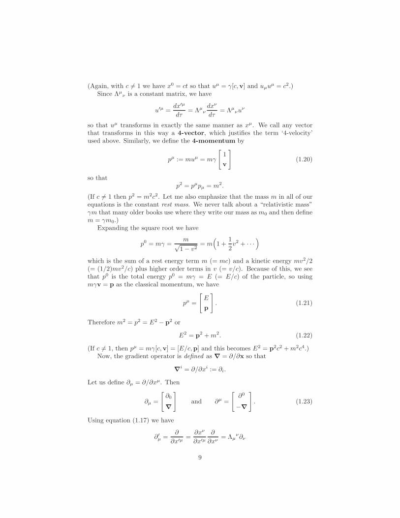
(Again, with c 6= 1 we have x0 = ct so that uµ = γ[c,v] and uµuµ = c2.)Since Λµ

ν is a constant matrix, we have

u′µ =dx′µ

dτ= Λµ

νdxν

dτ= Λµ

νuν

so that uµ transforms in exactly the same manner as xµ. We call any vectorthat transforms in this way a 4-vector, which justifies the term ‘4-velocity’used above. Similarly, we define the 4-momentum by

pµ := muµ = mγ

[

1

v

]

(1.20)

so thatp2 = pµpµ = m2.

(If c 6= 1 then p2 = m2c2. Let me also emphasize that the mass m in all of ourequations is the constant rest mass. We never talk about a “relativistic mass”γm that many older books use where they write our mass as m0 and then definem = γm0.)

Expanding the square root we have

p0 = mγ =m√

1 − v2= m

(

1 +1

2v2 + · · ·

)

which is the sum of a rest energy term m (= mc) and a kinetic energy mv2/2(= (1/2)mv2/c) plus higher order terms in v (= v/c). Because of this, we seethat p0 is the total energy p0 = mγ = E (= E/c) of the particle, so usingmγv = p as the classical momentum, we have

pµ =

[

E

p

]

. (1.21)

Therefore m2 = p2 = E2 − p2 or

E2 = p2 + m2. (1.22)

(If c 6= 1, then pµ = mγ[c,v] = [E/c,p] and this becomes E2 = p2c2 + m2c4.)Now, the gradient operator is defined as ∇ = ∂/∂x so that

∇i = ∂/∂xi := ∂i.

Let us define ∂µ = ∂/∂xµ. Then

∂µ =

[

∂0

∇

]

and ∂µ =

[

∂0

−∇

]

. (1.23)

Using equation (1.17) we have

∂′µ =

∂

∂x′µ=

∂xν

∂x′µ

∂

∂xν= Λµ

ν∂ν

9

or, equivalently,∂′µ = Λµ

ν∂ν

which shows that indeed ∂µ transforms as a 4-vector (which is implied by thenotation). The operator

∂µ∂µ = (∂0)2 + ∂i∂

i = (∂t)2 − ∇

2 =∂2

∂t2− ∇

2

is called the d’Alembertian, and is frequently written as �.In quantum mechanics we have the momentum operator defined by p =

−i~∇ and the energy operator defined by E = i~(∂/∂t). Then pi = −i~∇i =

−i~∂i = +i~∂i and we can define the relativistic momentum operator

pµ = i~∂µ.

Using units with ~ = 1, the expression E2 −p2 −m2 = 0 becomes −∂2t + ∇

2 −m2 = 0 or

(∂2t − ∇

2 + m2)φ(x) = (� + m2)φ(x) = 0

which is known as the Klein-Gordon equation.Even though the two reference frames relative to which we are describing

motion must be inertial, there is no reason we can’t describe the motion of anaccelerated object. As you might guess, we define the 4-acceleration of anobject by

aµ =duµ

dτ.

Since uµuµ = 1, it follows that the 4-acceleration is always orthogonal to the4-velocity because

0 =d

dτuµuµ = 2uµ

duµ

dτ= 2uµaµ.

We also define the 4-force

fµ =dpµ

dτ= maµ

so that

fµ =dpµ

dτ= γ

dpµ

dt= γ

[

d(γm)/dt

dp/dt

]

=

[

f0

γfc

]

(1.24)

where fc = dp/dt is the classical force on the particle. Since the 4-force obviouslyobeys fµuµ = 0, we have

0 = fµuµ = γf0 − γ2fc · v

and thereforef0 = γfc · v (1.25)

which, to within the factor of γ, is just the classical power (i.e., the rate atwhich work is done). (And if c 6= 1 we have 0 = fµuµ = f0γc − γ2fc · v so thatf0 = (γ/c)fc · v.)

10

2 Maxwell’s Equations

Experimentally, it is found that the charge to mass ratio e/mγ of a particlemoving at velocity β obeys the law

e

mγ=

e

m(1 − β2)1/2 .

(The two sides of this equation refer to different measurements, so it’s not as triv-ial of a statement as it looks at first.) Therefore, e is a constant, and we have thatcharge is an invariant quantity. What we would now like to know is how chargedensity and electric current behave. Since charge density is charge/volume, wemust find out how volumes transform.

Let frame 2 (the primed frame) be in motion with respect to frame 1 (theunprimed frame) along their mutual x-axis, and consider a small cube of sidel0 at rest in frame 2. In its rest frame, this cube has volume dτ0 (not to beconfused with proper time). From (1.7a) we have

dτ1 = dxdydz =1

γdx′dy′dz′ =

1

γdτ0 (2.1)

where we used dx′ = γ(dx− βdt) together with dt = 0 for a measurement madein frame 1. Thus we have

dτ1 = dτ0(1 − β2)1/2 .

Now suppose the volume is also moving with respect to frame 2, and let thismotion be along the x2 axis. Letting v2x be the velocity of the box with respectto frame 2, and similarly for v1x, we have

dτ2 = dτ0(1 − v22x)1/2 and dτ1 = dτ0(1 − v2

1x)1/2 .

But from (1.9b) we have

v1x =v2x + β

1 + βv2x

and therefore

dτ1 = dτ0

[

1 −(

v2x + β

1 + βv2x

)2]1/2

= dτ0

[

1 + 2βv2x + β2v22x − v2

2x − 2βv2x − β2

(1 + βv2x)2

]1/2

= dτ0

[

(1 − β2)(1 − v22x)

(1 + βv2x)2

]1/2

= dτ0[(1 − β2)(1 − v2

2x)]1/2

1 + βv2x

=(1 − β2)1/2

1 + βv2xdτ2

11

where in going to the last line we used dτ2 = dτ0(1− v22x)1/2. Rearranging, this

is

dτ1 =dτ2

γ(1 + βv2x). (2.2a)

Reversing the frame point of view, we clearly also have

dτ2 =dτ1

γ(1 − βv1x). (2.2b)

Be sure to understand what these equations say. The velocities v1x and v2x arethe observed velocities of a box with rest volume dτ0 moving along the commonx-axis as seen in frames 1 and 2, which are moving with velocity β with respectto each other.

Now suppose that we have dn charges of Q coulombs each. As we statedabove, Q is an invariant. Obviously, dn is also an invariant since it is just thenumber of charges. Then the charge densities as observed in frames 1 and 2 are

ρ1 =Q dn

dτ1and ρ1 =

Q dn

dτ1

so thatρ1 dτ1 = ρ2 dτ2

where dτ1 and dτ2 are the same volume containing the charge Q dn as observedin the two different reference frames. Then, using equations 2.2, we have

ρ1 = ρ2dτ2

dτ1= ρ2γ(1 + βv2x)

ρ2 = ρ1dτ1

dτ2= ρ1γ(1 − βv1x) .

(2.3)

The current density J := ρv is defined as the charge per area-time, so wecan write J1x = ρ1v1x and J2x = ρ2v2x. Using these definitions in equations(2.3) yields the transformation of charge density

ρ1 = γ(ρ2 + βJ2x)

ρ2 = γ(ρ1 − βJ1x) .(2.4)

Now using equations (1.9) and (2.3) we also have

J1x = ρ1v1x = ρ2γ(1 + βv2x)v2x + β

1 + βv2x

or

J1x = γ(J2x + βρ2)

J2x = γ(J1x − βρ1) .(2.5a)

Similarly,J1y = ρ1v1y = ρ2γ(1 + βv2x)v1y .

12

But

v1y =dy1

dt1=

dy2

γ(dt2 + βdx2)=

v2y

γ(1 + βv2x).

HenceJ1y = ρ2v2y = J2y and similarly J1z = J2z . (2.5b)

Comparing equations (2.4) and (2.5) with equations (1.7), we see that we havea 4-current density

Jµ =

[

ρ

J

]

. (2.6)

(And again, if c 6= 1 this becomes Jµ = [ρc,J].)Now that we have shown that Jµ does indeed define a 4-vector, let me show

another way to arrive at this conclusion that is analogous to the definition of4-momentum. From (2.1) we can write dτ = dτ0/γ where dτ0 is at rest in frame2, and γ = (1−β2)−1/2 where β is the velocity of frame 2 with respect to frame1. Then the invariance of charge implies ρdτ = ρ0dτ0 or ρdτ0/γ = ρ0dτ0, andhence

ρ = γρ0 .

This is analogous to the expression mrelativistic = γmrest or simply m = γm0.Now we also have J = ρv = ρ0γv. Recalling that the 4-velocity is given by

uµ =

[

γ

γv

]

we see that letting v be the velocity of the charge, i.e., v = β, then (2.6) is thesame as

Jµ = ρ0uµ

which is analogous to pµ = muµ. In other words, we have shown

Jµ =

[

ρ

J

]

= ρ0

[

γ

γv

]

= ρ0uµ . (2.7)

Since we saw earlier that the derivative operator ∂µ transforms as a 4-vector(technically, a co-vector), and we just showed that Jµ is a 4-vector, it followsthat ∂µJµ is a Lorentz scalar. But

∂µJµ = ∂0ρ + ∂iJi =

∂ρ

∂t+ ∇ · J

and therefore the continuity equation may be written in the covariant form

∂µJµ = 0 . (2.8)

13

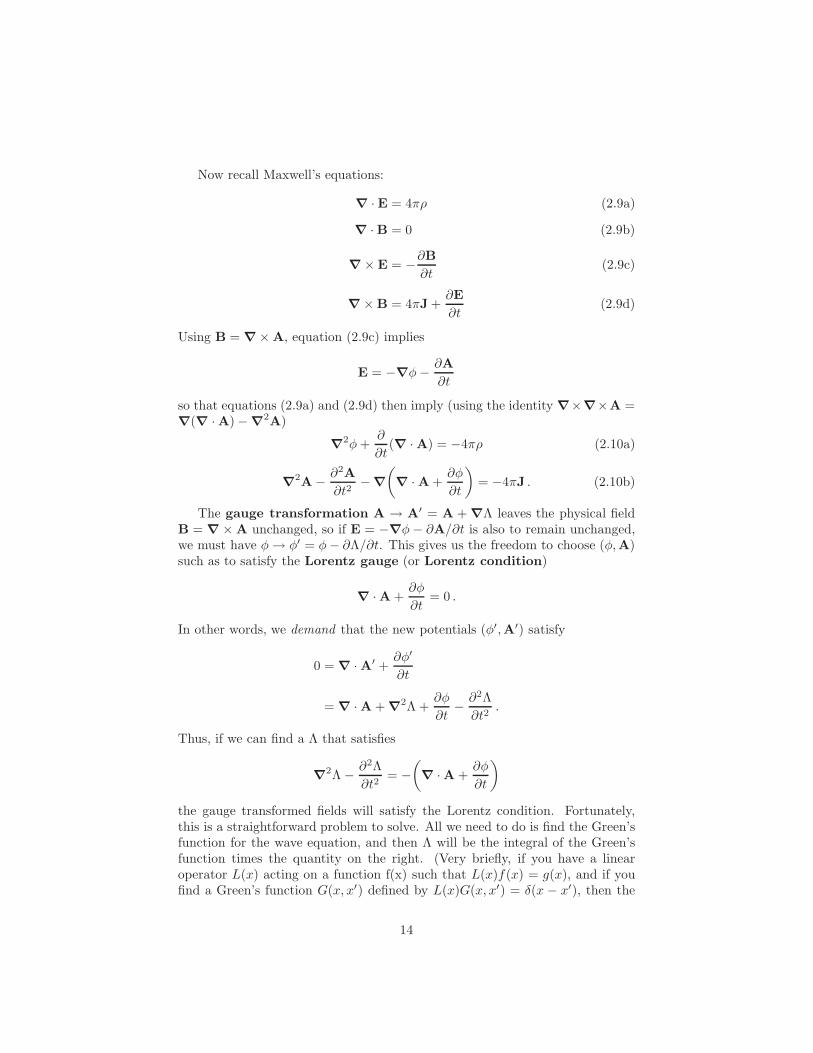
Now recall Maxwell’s equations:

∇ ·E = 4πρ (2.9a)

∇ ·B = 0 (2.9b)

∇ × E = −∂B

∂t(2.9c)

∇ × B = 4πJ +∂E

∂t(2.9d)

Using B = ∇ × A, equation (2.9c) implies

E = −∇φ − ∂A

∂t

so that equations (2.9a) and (2.9d) then imply (using the identity ∇×∇×A =∇(∇ ·A) − ∇

2A)

∇2φ +

∂

∂t(∇ · A) = −4πρ (2.10a)

∇2A − ∂2A

∂t2− ∇

(

∇ · A +∂φ

∂t

)

= −4πJ . (2.10b)

The gauge transformation A → A′ = A + ∇Λ leaves the physical fieldB = ∇ × A unchanged, so if E = −∇φ − ∂A/∂t is also to remain unchanged,we must have φ → φ′ = φ − ∂Λ/∂t. This gives us the freedom to choose (φ,A)such as to satisfy the Lorentz gauge (or Lorentz condition)

∇ ·A +∂φ

∂t= 0 .

In other words, we demand that the new potentials (φ′,A′) satisfy

0 = ∇ · A′ +∂φ′

∂t

= ∇ · A + ∇2Λ +

∂φ

∂t− ∂2Λ

∂t2.

Thus, if we can find a Λ that satisfies

∇2Λ − ∂2Λ

∂t2= −

(

∇ ·A +∂φ

∂t

)

the gauge transformed fields will satisfy the Lorentz condition. Fortunately,this is a straightforward problem to solve. All we need to do is find the Green’sfunction for the wave equation, and then Λ will be the integral of the Green’sfunction times the quantity on the right. (Very briefly, if you have a linearoperator L(x) acting on a function f(x) such that L(x)f(x) = g(x), and if youfind a Green’s function G(x, x′) defined by L(x)G(x, x′) = δ(x − x′), then the

14

solution to the problem is essentially f(x) =∫

G(x, x′)g(x′) dx′. You can easilyverify that acting on this with L(x) will yield L(x)f(x) = g(x).)

In any case, choosing the Lorentz gauge, equations (2.10) become the well-known wave equations

∇2φ − ∂2φ

∂t2= −4πρ (2.11a)

∇2A− ∂2A

∂t2= −4πJ . (2.11b)

Note that an equivalent way of writing these is

�φ = −4πJ0

�A = −4πJ .

So if we define the 4-potential Aµ by

Aµ =

[

φ

A

]

then the wave equations may be written in the concise form

�Aµ = −4πJµ (2.12)

where the Lorentz condition becomes

∂µAµ = 0 .

That Aµ is indeed a 4-vector follows because � is a Lorentz invariant quantityand Jµ is a 4-vector. Thus Aµ must transform as a 4-vector so that (2.12)is covariant (i.e., so that both sides transform the same way). Also, Aµ isunchanged even if c 6= 1. This is because the right side of (2.11b) becomes(−4π/c)J and J0 = ρc.

Now we need a bit of terminology. Recall that a 4-vector was defined as aquantity vµ that under a Lorentz transformation transformed as

vµ → v′µ = Λµνvν .

As we shall see below, it is also possible to have quantities with more than oneindex such that under a Lorentz transformation, each index transforms like a4-vector. For example, a quantity Fµν (not necessarily the electromagnetic fieldtensor) with two indices that transforms like

Fµν → F ′µν = ΛµαΛν

βFαβ

is called a (second rank) tensor. Higher rank tensors are defined in the obviousmanner. Note also that all of the indices need not be superscripts (such indices

15

are called contravariant). We can equally have subscripts (called covariant)that transform like

F ′µν = Λµ

αΛνβFαβ .

And we can have a mixed tensor like Fµν . Indices are raised and lowered by

using the metric gµν and its inverse gµν .At last we are ready to write Maxwell’s equations in covariant form. It is

not hard to show that even though ∂µ transforms as a 4-vector under a Lorentztransformation Λµ

ν , as does Aµ, the quantity ∂µAν does not transform as asecond-rank tensor. However, the antisymmetric quantity Fµν defined by

Fµν := ∂µAν − ∂νAµ (2.13a)

does indeed transform as a tensor. This is called the electromagnetic field

tensor. Equivalently, we may consider the contravariant version

Fµν = ∂µAν − ∂νAν . (2.13b)

I claim that equations (2.9a) and (2.9d) can be written in the form

∂µFµν = Jν . (2.14)

To see this, first recall that we are using the metric g = diag(1,−1,−1,−1)so that ∂/∂t = ∂/∂x0 = ∂0 = ∂0 and ∇

i := ∂/∂xi = ∂i = −∂i. UsingE = −∇ϕ − ∂A/∂t we have

Ei = ∂iA0 − ∂0Ai = F i0

and also B = ∇ × A so that

B1 = ∇2A3 − ∇

3A2 = −∂2A3 + ∂3A2 = −F 23

plus cyclic permutations 1 → 2 → 3 → 1. Then the electromagnetic field tensoris given by

Fµν =

0 −E1 −E2 −E3

E1 0 −B3 B2

E2 B3 0 −B1

E3 −B2 B1 0

. (2.15)

(Be sure to note that this is the form of Fµν for the metric diag(1,−1,−1,−1).If you use the metric diag(−1, 1, 1, 1) then all entries of Fµν change sign. Inaddition, you frequently see the matrix Fµ

ν which also has different signs.)Now, for the ν = 0 component of (2.14) we have

J0 = ∂µFµ0 = ∂iFi0 = ∂iE

i

which is Coulomb’s law∇ · E = ρ .

16

Next consider the ν = 1 component of (2.14). This is

J1 = ∂µFµ1 = ∂0F01 + ∂2F

21 + ∂3F31

= −∂0E1 + ∂2B

3 − ∂3B2

= −∂tE1 + (∇ × B)1

and therefore we have

∇ × B− ∂E

∂t= J .

Finally, I leave it as an exercise for you to show that equations (2.9b) and(2.9c) can be written as (note the superscripts are cyclic permutations)

∂µF νσ + ∂νF σµ + ∂σFµν = 0

or simply∂[µF νσ] = 0 . (2.16)

Remark: There is another interesting way to arrive at the electromagnetic fieldtensor that we now describe, but you are free to skip over it. First we need togive a more careful definition of a tensor. To begin, given a vector space V , wecan define the dual space V ∗ as the vector space of linear functionals on V .In other words, α ∈ V ∗ means that α : V → R is a linear map from V to R.(We restrict consideration to real vector spaces.) Members of the dual spaceare frequently called covectors. If V has a basis {e1, . . . , en}, we define the nlinear functionals {ω1, . . . , ωn} by

ωi(ej) = δij .

I will show that these n linear functionals form a basis for V ∗, i.e., that theyare linearly independent and span V ∗.

To show this, let α ∈ V ∗ be arbitrary but fixed. Note that for any v ∈ V ,using the linearity of α we have

α(v) = α(viei) = viα(ei) = aivi

where we have defined the scalars ai by ai = α(ei). On the other hand,

ωi(v) = ωi(vjej) = vjωi(ej) = vjδij = vi

and hence we see that α(v) = aivi = aiω

i(v) so that α = aiωi. This shows that

the ωi span V ∗.To show they are linearly independent, suppose we have ciω

i = 0 for someset of scalars ci. Then for any j = 1, . . . , n we have 0 = ciω

i(ej) = ciδij = cj

which proves linear independence. Thus we have shown that any α ∈ V ∗ canbe written in the form

α = aiωi = α(ei)ω

i .

17

As an example, consider the space V = R2 consisting of all column vectors

of the form

v =

[

v1

v2

]

.

Relative to the standard basis we have

v = v1

[

10

]

+ v2

[

01

]

= v1e1 + v2e2.

If φ ∈ V ∗, then φ(v) =∑

φivi, and we may represent φ by the row vector

φ = (φ1, φ2). In particular, if we write the dual basis as ωi = (ai, bi), then wehave

1 = ω1(e1) = (a1, b1)

[

10

]

= a1

0 = ω1(e2) = (a1, b1)

[

01

]

= b1

0 = ω2(e1) = (a2, b2)

[

10

]

= a2

1 = ω2(e2) = (a2, b2)

[

01

]

= b2

so that ω1 = (1, 0) and ω2 = (0, 1). Note, for example,

ω1(v) = (1, 0)

[

v1

v2

]

= v1

as it should.As another very important example, let V be an inner product space. If

a, b ∈ V , then the inner product of a and b is the number 〈a, b〉. Then given afixed vector a, the quantity 〈a, ·〉 is a linear functional on V because it takes avector b ∈ V and gives back a number:

〈a, ·〉 : b → 〈a, b〉 ∈ R .

Since 〈a, ·〉 is in V ∗, let us denote it by α, so that α(b) = 〈a, b〉.Given a basis {ei} for V , let us define the numbers gij by

gij := 〈ei, ej〉 = 〈ej , ei〉 = gji .

This is the proper definition of the metric. Then

〈a, b〉 = 〈aiei, bjej〉 = aibj〈ei, ej〉 = aibjgij = bjgjia

i .

But we also haveα(b) = α(bjej) = bjα(ej) = bjaj

18

and thereforebjaj = α(b) = 〈a, b〉 = bjgjia

i .

Hence we defineaj = gjia

i .

This is called lowering an index.Since the inner product is nondegenerate by definition, the metric gij must

be nonsingular, and hence we can define its inverse which we denote by gij .Multiplying this last equation by gkj we then have

gkjaj = gkjgjiai = δk

i ai = ak

and thus we define raising an index by

ak = gkjaj .

Now that we have an understanding of dual spaces, we are in a position todefine tensors carefully. So, a tensor T is just a multilinear map

T : V ∗s × V r = V ∗ × · · · × V ∗ × V × · · · × V → R .

By multilinear, we mean that it is linear in each variable separately. This tensoris said to have covariant order r, and contravariant order s, or simply to be atensor of type (s, r). In other words, T takes as its argument s covectors andr vectors. Since it is multilinear, we see that

T (α(1), . . . , α(s), v(1), . . . ,v(r))

= T (a(1)i1

ωi1 , . . . , a(s)is

ωis , vj1(1)ej1 , . . . , v

ir

(r)eir)

= a(1)i1

· · · a(s)is

vj1(1) · · · v

jr

(r)T (ωi1 , . . . , ωis , ej1 , . . . , ejr)

= a(1)i1

· · · a(s)is

vj1(1) · · · v

jr

(r)Ti1···is

j1···jr

where the last line defines the components of T . Thus we see that if we know thecomponents of T , then we know the result of T acting on an arbitrary collectionof vectors and covectors.

What happens to the components of T under a change of coordinates? Froma practical standpoint, this is what really defines a tensor. A change of basis inV is of the form

ei → ei = ejpji

where (pji) is called the transition matrix. Then any x ∈ V can be written

in terms of its components with respect to either ei or ei, and we have

x = xjej = xiei = xiejpji

and therefore we must havexj = pj

ixi

19

orxi = (p−1)i

jxj .

From these we easily see that

pij =

∂xi

∂xjand (p−1)i

j =∂xi

∂xj.

When V undergoes a change of basis, what about V ∗? Let us write in generalωi → ωi = bi

jωj . Since we must also have ωi(ej) = δi

j , we see that

δij = ωi(ej) = ωi(ekpk

j) = pkjω

i(ek) = pkjb

ilω

l(ek) = pkjb

ilδ

lk = bi

kpkj

so that bik = (p−1)i

k. In other words,

ωi → ωi = (p−1)ijω

j .

Finally we are in a position to derive the general transformation law of atensor. We have

Ti1···is

j1···jr= T (ωi1 , . . . , ωis , ej1 , . . . , ejr

)

= T ((p−1)i1k1

ωk1 , . . . , (p−1)is

ks

ωks , el1pl1

j1 , . . . , elrplr

jr

)

= (p−1)i1k1

· · · (p−1)is

ks

pl1j1 · · · plr

jr

T (ωk1 , . . . , ωks , el1 , . . . , elr)

= (p−1)i1k1

· · · pl1j1 · · ·T

k1···ks

l1···lr

or

Ti1···is

j1···jr=

∂xi1

∂xk1

· · · ∂xis

∂xks

∂xl1

∂xj1· · · ∂xlr

∂xjr

T k1···ks

l1···lr .

This is the classical transformation law of a type (s, r) tensor.In the particular case of a second rank tensor Fµν under a Lorentz transfor-

mation, we havexµ = Λµ

νxν

so that∂xµ

∂xν= Λµ

ν

and therefore

Fµν

=∂xµ

∂xα

∂xν

∂xβFαβ = Λµ

αΛνβFαβ .

Let us now return to the physics. We know that the Lorentz force law is

F = q(E + v × B) =dp

dt

so consider (now τ is the proper time again)

dp

dτ=

dt

dτ

dp

dt= γ

dp

dt.

20

In terms of the 4-velocity

uµ =

[

γ

γv

]

=

[

u0

u

]

we can write

dp

dτ= γq(E + v × B) = q(γE + γv × B)

= q(u0E + u× B) . (2.17)

Also note that if W = p0 is the energy of the particle, then the change inenergy is the rate at which work is done, so that

dW

dt= F · dr

dt= F · v = q(E + v × B) · v = qE · v

and thereforedp0

dτ=

dW

dτ= γ

dW

dt= qE · γv = qE · u . (2.18)

Combining equations (2.17) and (2.18), we see that we can define a linearmap uµ → dpµ/dτ of a 4-vector to another 4-vector, and hence there exists asecond rank mixed tensor Fµ

ν such that

dpµ

dτ= qFµ

νuν . (2.19)

Comparing (2.19) with (2.17) and (2.18) allows us to pick out the componentsof Fµ

ν :

Fµν =

0 Ex Ey Ez

Ex 0 Bz −By

Ey −Bz 0 Bx

Ez By −Bx 0

.

Finally, we note that we can also write Fµν in the alternate forms Fµν = gµαFα

ν

and Fµν = gναFµα.

Now that we have the electromagnetic field tensor, it is straightforward toderive the transformation laws for the E and B fields. Starting from Fµν whichdefines the fields E and B, we have F ′µν = Λµ

αΛνβFαβ which then gives the

fields E′ and B′ in terms of E and B. In matrix notation, we can write this as

F ′ = ΛFΛT .

Using equations (1.14) and (2.15), it is easy to multiply out the matrices and

21

show that

F ′µν =

0 −E′1 −E′2 −E′3

E′1 0 −B′3 B′2

E′2 B′3 0 −B′1

E′3 −B′2 B′1 0

=

0 −E1 −γ(E2 − βB3) −γ(E3 + βB2)

E1 0 −γ(B3 − βE2) γ(B2 + βE3)

γ(E2 − βB3) γ(B3 − βE2) 0 −B1

γ(E3 + βB2) −γ(B2 + βE3) B1 0

.

This was for the special case of a boost along the x-axis, i.e., β = βx. itis not hard to see that we can write down the field transformation laws for aboost β in an arbitrary direction (but with the coordinate axes still parallel) ifwe write this in terms of components parallel and perpendicular to the boost.This yields

E′⊥ = γ(E⊥ + β × B) E′

‖ = E‖ (2.20a)

B′⊥ = γ(B⊥ − β × E) B′

‖ = B‖ (2.20b)

22