special issue on leonhard paul euler’s: functional and...
TRANSCRIPT

Special Issue on Leonhard Paul Euler’s:
Functional and Differential Equations (F. D. E.)
Volume 9 Number J07 June 2007
ISSN 0973-1377 (Print)ISSN 0973-7545 (Online)

International Journal of AppliedMathematics & Statistics
ISSN 0973-1377 (Print), ISSN 0973-7545 (Online)
Editorial Board
Executive Editor:
Tanuja Srivastava Department of Mathematics,
Indian Institute of Technology Roorkee-247667,INDIA
Email: [email protected]
Editors-in-Chief:
Florentin Smarandache Department of Mathematics & Sciences, University of New Mexico, USA. E-mail: [email protected]
R. K. S. Rathore
Department of Mathematics, Indian Institute of Technology, Kanpur, INDIA E-mail: [email protected]
Editors
Delfim F. M. Torres University of Aveiro Portugal Alexandru Murgu British Tel. Net. Research Centre UK Edward Neuman Southern Illinois University USA Hans Gottlieb Griffith University Australia Akca Haydar United Arab Emiartes University UAE Somesh Kumar Indian Institute of Technology, Kharagpur India
Associate Editors:
Alexander Grigorash University of Ulster U.K.
Bogdan G. Nita Montclair State University USA
Sukanto Bhattacharya Alaska Pacific University USA
Rogemar S Mamon University of Western Ontario Canada
Ferhan Atici Western Kentucky University USA
Karen Yagdjian University of Texas-Pan American USA
Rui Xu University of West Georgia USA
Alexander A. Katz St. John's University USA

Associate Editors: Contd….
Eduardo V. Teixeira Rutgers University USA
Weijiu Liu University of Central Arkansas USA
Wieslaw A. Dudek Wroclaw University of Technology Poland
Ki-Bong Nam University of Wisconsin, Whitewater USA
Diego Ernesto Dominici State University of New York at New Paltz USA
Ming Fang Norfolk State University USA
Hemant Pendharkar Worcester State College USA
Wen-Xiu Ma University of South Florida USA
V. Ravichandran University Sains Malaysia Malaysia
Piotr Matus Institute of Mathematics of NASB Belarus
Mustafa Bayram Yildiz Teknik Üniversitesi Turkey
Rodrigo Capobianco Guido University of S.ao Paulo Brazil
Song Wang University of Western Australia Australia
Tianzi Jiang Institute of Automation, CAS PR China
Henryk Fuks Brock University Canada
Nihal Yilmaz Ozgur Balikesir University Turkey
Muharem Avdispahic University of Sarajevo Bosnia
Xiao-Xiong Gan Morgan State University USA
Assistant Editors:
Irene Sciriha University of Malta Malta Doreen De Leon California State University USA Anahit Ann Galstyan University of Texas-Pan American USA Oliver Jones California State University USA Jose Almer T. Sanqui Appalachian State University USA Miranda I. Teboh-Ewungkem Lafayette College USA Guo Wei University of North Carolina at Pembroke USA Michael D. Wills Weber State University USA Alain S. Togbe Purdue University North Central USA Samir H. Saker Mansoura University Egypt Ganatsiou V. Chrysoula University of Thessaly Greece Bixiang Wang New Mexico Institute of Mining & Technology USA Andrei Volodin University of Regina Canada Mohammad Sal Moslehian Ferdowsi University Iran Ashwin Vaidya University of North Carolina - Chapel Hill USA Anna Karczewska University of Zielona Góra Poland Xiaoli Li University of Birmingham UK Guangyi Chen Canadian Space Agency Canada Clemente Cesarano University of Roma Italy Rãzvan Rãducanu Al. I. Cuza University Romania Fernando M. Lucas Carapau University of Évora Portugal Alireza Abdollahi University of Isfahan Iran Ay e Altın Hacettepe University Turkey

Special Issue on Leonhard Paul Euler’s:
Functional and Differential Equations (F. D. E.)
Special Editor-in-Chief
John Michael Rassias
Professor of Mathematics, National and Capodistrian, University of Athens, Greece
Guest Editors
Jewgeni H. Dshalalow Florida Institute of Technology, Division of Mathematical Sciences,
College of Science, Melbourne, FL 32901, U. S. A.
Valerii A. Faiziev Tver State Agricultural Academy, Tver Sakharovo, RUSSIA
David Goss The Ohio State University, Department of Mathematics
231 W. 18th Ave., Columbus, Ohio 43210, U. S. A.
Johnny Henderson Baylor University, Department of Mathematics
Waco, Texas 76798-7328, U. S. A.
T. Kusano Fukuoka University, Department of Applied Mathematics,
Faculty of Science, Fukuoka, 814-0180, JAPAN
Alexander G. Kuz’min St Petersburg State University
Institute of Mathematics and Mechanics 28 University Ave., 198504 St Petersburg, RUSSIA
Xuerong Mao University of Strathclyde
Department of Statistics and Modelling Science, Glasgow G1 1XH, U. K.
Shuji Watanabe Gunma University
Department of Mathematics, Faculty of Engineering 4-2 Aramaki-machi, Maebashi 371-8510, JAPAN
Guochun Wen Peking University
School of Mathematical Sciences, Beijing 100871, CHINA

International Journal of Applied Mathematics & Statistics
Contents
Volume 9 Number J07 June 2007
Preface 6
An Iterative Method for the Computation of Eigenpairs of Singular Sturm-Liouville Problems
B.S. Attili
8
Euler-type Boundary Value Problems in Quantum Calculus
Martin Bohner and Thomas Hudson
19
Positive Solutions of Third Order Boundary Value Problems
Abdelkader Boucherif
24
Controllability of Nondensely Defined Impulsive Functional Semilinear Differential Inclusions in Frechet Spaces
Johnny Henderson and Abdelghani Ouahab
35
Asymptotic properties of nonoscillatory proper solutions of the Emden-Fowler equation
N. A. Izobov and V. A. Rabtsevich
55
Comparison Theorems for Perturbed Half-linear Euler Differential Equations
T. Kusano, J. Manojlovic and T. Tanigawa
77
Almost Sure Asymptotic Estimations for Solutions of Stochastic Differential Delay Equations
Xuerong Mao and Matina John Rassias
95
A Class of Second Order Difference Equations Inspired by Euler’s Discretization Method
H. Sedaghat and M. Shojaei
110
Extended Oligopoly Models and Their Asymptotical Behavior
F. Szidarovszky
124
PREFACE
This Euler’s commemorating volume entitled : Functional Equations , Integral Equations, Differential Equations and Applications (F. I. D. A),is a forum for exchanging ideas among eminent mathematicians and physicists, from many parts of the world, as a tribute to the tri-centennial birthday anniversary of Leonhard Paul Euler (April 15,1707 A.D., b. in Basel – September 18, 1783 A.D., d. in St. Petersburg). This 998 pages long collection is composed of outstanding contributions in mathematical and physical equations and inequalities and other fields of mathematical, physical and life sciences. In addition, this anniversary volume is unique in its target, as it strives to represent a broad and highly selected participation from across and beyond the scientific and technological country regions. It is intended to boost the cooperation among mathematicians and physicists working on a broad variety of pure and applied mathematical areas. Moreover, this new volume will provide readers and especially researchers with a detailed overview of many significant insights through advanced developments on Euler’s mathematics and physics. This transatlantic collection of mathematical ideas and methods comprises a wide area of applications in which equations, inequalities and computational techniques pertinent to their solutions play a core role.Euler’s influence has been tremendous on our everyday life, because new tools have been developed, and revolutionary research results have been achieved , bringing scientists of exact sciences even closer, by fostering the emergence of new approaches, techniques and perspectives. The central scope of this commemorating 300birthday anniversary volume is broad, by deeper looking at the impact and the ultimate role of mathematical and physical challenges, both inside and outside research institutes, scientific foundations and organizations. We have recently observed a more rapid development in the areas of research of Euler worldwide. Leonhard P. Euler (1707-1783) was actually the most influential mathematician and prolific writer of the eighteenth century, by having contributed to almost all the fundamental fields of mathematics and mathematical physics. In calculus of variations, according to C. Caratheodory, Euler’s work: Methodus inveniendi lineas curves…(1740 A.D.) was one of the most beautiful works ever written. Euler was dubbed Analysis Incarnate by his peers for his incredible ability. He was especially great from his writings and that produced more academic work on mathematics than anyone. He could produce an entire new mathematical paper in about thirty minutes and had huge piles of his works lying on his desk. It was not uncommon to find Analysis Incarnate ruminating over a new subject with a child on his lap. This volume is suitable for graduate students and researchers interested in functional equations, integral equations and differential equations and would make an ideal supplementary reading or independent study research text. This item will also be of interest to those working in other areas of mathematics and physics. It is a work of great interest and enjoyable read as well as unique in market.
This Euler’s volume (F. I. D. A.) consists of six (6) issues containing various parts of contemporary pure and applied mathematics with emphasis to Euler’s mathematics and physics. It contains sixty eight (68) fundamental research papers of one hundred one (101) outstanding research contributors from twenty seven (27) different countries. In particular, these contributors come from: Algerie (1 contributor); Belgique (2); Bosnia and Herzegovina (2); Brazil (2); Bulgaria (3); China (9); Egypt (1); France (3); Greece (2); India (8); Iran (3); Italy (1); Japan (7); Korea (7); Morocco (3); Oman (2); Poland (3); R. O. Belarus (8); Romania (2); Russia (3); Saudi Arabia (1); Serbia and Montenegro (5); The Netherlands (3); U. A. Emirates (1);U. K. (2); U. S. A. (15); Uzbekistan (2).
First Issue (F. E. I.) consisting of 14 research papers, 181 pages long, contains various parts of Functional Equations and Inequalities,namely:Euler’s Life and Work, Ulam stability, Hyers – Ulam stability and Ulam – Gavruta - Rassias stability of functional equations, Euler – Lagrange type and Euler – Lagrange – Rassias quadratic mappings in Banach and Hilbert spaces, Aleksandrov and isometry Ulam stability problems, stability of Pexider and Drygas functional equations, alternative of fixed point, and Hyers - Ulam stability of differential equations.
International Journal of Applied Mathematics & Statistics,ISSN 0973-1377 (Print), ISSN 0973-7545 (Online)Copyright © 2007 by IJAMAS, CESER IJAMAS: June 2007, Vol. 9, No. J07, 6-7

Second Issue (MT. PDE) consisting of 9 research papers, 117 pages long, contains various parts of Mixed Type Partial Differential Equations,namely:Tricomi - Protter problem of nD mixed type partial differential equations, solutions of generalized Rassias’ equation, degenerated elliptic equations, mixed type oblique derivative problem, Cauchy problem for Euler – Poisson - Darboux equation, non - local boundary value problems, non-uniqueness of transonic flow past a flattened airfoil, multiplier methods for mixed type equations. Third Issue (F . D . E.) consisting of 9 research papers, 146 pages long, contains various parts of Functional and Differential Equations,namely:Iterative method for singular Sturm - Liouville problems, Euler type boundary value problems in quantum mechanics, positive solutions of boundary value problems, controllability of impulsive functional semi-linear differential inclusions in Frechet spaces, asymptotic properties of solutions of the Emden-Fowler equation, comparison theorems for perturbed half-linear Euler differential equations, almost sure asymptotic estimations for solutions of stochastic differential delay equations, difference equations inspired by Euler’s discretization method, extended oligopoly models. Fourth Issue (D. E. I.) consisting of 9 research papers, 160 pages long, contains various parts of Differential Equations and Inequalities,namely:New spaces with wavelets and multi-fractal analysis, mathematical modeling of flow control and wind forces, free convection in conducting fluids, distributions in spaces, strong stability of operator– differential equations, slope – bounding procedure, sinc methods and PDE, Fourier type analysis and quantum mechanics. Fifth Issue (DS. IDE.) consisting of 9 research papers, 159 pages long, contains various parts of Dynamical Systems and Integro - Differential Equations,namely:Semi-global analysis of dynamical systems, nonlinear functional-differential and integral equations, optimal control of dynamical systems, analytical and numerical solutions of singular integral equations, chaos control of classes of complex dynamical systems, second order integro-differential equation, integro-differential equations with variational derivatives generated by random partial integral equations, inequalities for positive operators, strong convergence for a family of non-expansive mappings. Sixth Issue (M. T. A.) consisting of 18 research papers, 231 pages long, contains various parts of Mathematical Topics and Applications,namely:Maximal subgroups and theta pairs in a group, Euler constants on algebraic number fields, characterization of modulated Cox measures on topological spaces, hyper-surfaces with flat r-mean curvature and Ribaucour transformations, Leonhard Euler’s methods and ideas live on in the thermodynamic hierarchical theory of biological evolution, zeroes of L-series in characteristic p, Beck’s graphs, best co-positive approximation function, Convexity in the theory of the Gamma function, analytical and differential – algebraic properties of Gamma function, Ramanujan’s summation formula and related identities, ill – posed problems, zeros of the q-analogues of Euler polynomials, Eulerian and other integral representations for some families of hyper-geometric polynomials, group C*-algebras and their stable rank, complementaries of Greek means to Gini means, class of three- parameter weighted means, research for Bernoulli’s inequality.
Deep gratitude is due to all those Guest Editors and Contributors who helped me to carry out this intricate project. My warm thanks to my family: Matina- Mathematics Ph. D. candidate of the Strathclyde University (Glasgow, United Kingdom), Katia- Senior student of Archaeology and History of Art of the National and Capodistrian University of Athens (Greece), and Vassiliki- M. B. A. of the University of La Verne, Marketing Manager in a FMCG company (Greece). Finally I express my special appreciation to: The Executive Editor of the International Journal of Applied Mathematics & Statistics (IJAMAS)Dr. Tanuja Srivastava for her nice cooperation and great patience.
John Michael Rassias
Special Editor-in-Chief of Euler’s volume F. I. D. A. – IJAMAS.National and Capodistrian University of Athens, Greece E-mail: [email protected]; [email protected] URL: http://www.primedu.uoa.gr/~jrassias/
Int. J. Appl. Math. Stat.; Vol. 9, No. J07, June 2007 7
An Iterative Method for the Computation of Eigenpairs ofSingular Sturm-Liouville Problems
B.S. Attili
Mathematical Sciences DepartmentUnited Arab Emirates University
P. O. Box 17551, Al-Ain, [email protected]
ABSTRACT
We propose an iterative method coupled with simple shooting for computing the eigenpairs
of singular Sturm-Liouville problems. The problem is first transformed into a regular initial
value problem which is then solved using standard numerical methods. The accuracy of
the proposed iterative method per step is the same as that of the IVP solver. Numerical
examples will be presented to demonstrate the efficiency of the method.
Keywords: Eigenpairs, Sturm-Liouville, Singular B. V. P’s.
2000 Mathematics Subject Classification: 65N25.
1 Introduction
It is well known that the study of Sturmian theory is an important aid in solving numerous
problems in mathematical physics, thermodynamics, electrostatics, quantum mechanics and
statistics. These sciences are rich source of the eigenvalue problems that are termed ”Sturm-
Liouville” two point boundary value problems of the form
− (py′)′ + qy = λwy (1.1)
on some interval (a, b) of the real line subject to some boundary conditions. Very often and in
applications singularities are encountered at one or more points in that interval. For example
equations having the form given in (1.1) appears when separation of variables is attempted on
the heat equation in a solid sphere or the electrostatic potential in the sphere. The source of
the singularity in this case is the vanishing of the function p at the endpoints.
When applied to the singular problems of the form (1.1), standard numerical methods designed
for regular ordinary differential equations will have difficulties in terms of convergence and
suffer from a loss of accuracy. In some cases they may even fail to converge [2]. For that
reason, special numerical methods have been proposed to handle the singular problem. Such
proposed methods converge, some with a lesser order of convergence due to the singularity
and some under various assumptions on the data, may retain the standard rate of convergence
in the regular case. We refer to [3, 6, 8] and the references therein for more on this point.
International Journal of Applied Mathematics & Statistics,ISSN 0973-1377 (Print), ISSN 0973-7545 (Online)Copyright © 2007 by IJAMAS, CESER IJAMAS: June 2007, Vol. 9, No. J07, 8-18
Many authors considered the Sturm-Liouville problem both the singular and the regular cases.
For example polynomial Sturm-Liouville problems were considered by [1], singular problems
with rational coefficients was considered by [10] while regular and singular problems were
studied extensively by [11, 12, 13, 16, 17]. Some theoretical results can be found for example
[2, 7, 14, 15].
In this work we propose an iterative method, coupled with simple shooting for the numerical
solution of (1.1). In each step of the iteration we solve a regular ODE and, therefore, may use
standard numerical methods. Thus the accuracy of the proposed iterative method per step is
the same as the accuracy of the numerical ODE solver used, see [8].
The outline of the paper is as follows. In Section 2 some preliminary results are given to set up
the terminology and state the class of the boundary value problems to be numerically treated.
We discuss the applicability of the simple shooting method to this class of singular boundary
value problems in Section 3. In Section 4 we introduce the iterative method and discuss its
justification. Some numerical examples are given in the last section.
2 Preliminaries
Before considering the Sturm-Liouville eigenvalue problem further, it is worth mentioning that
a general second order linear ordinary differential equation of the form
P (x)u′′ + Q(x)u′ + (R(x) + λ)u = 0
can be transformed to Sturm-Liouville problem which has the form
− (p(x)u′)′ + [q(x) + λw(x)]u = 0. (2.1)
This can be done by first dividing by P (x) and then multiplying by the integrating factor given
by e∫ x Q
Pdt.
It is amazing how much information one can infer about the eigenvalues and eigenfunctions
of a Surm-Liouville problem without actually solving the differential equation explicitly. Thus
from very general and simple considerations, one can discover that the eigenvalues are real,
are discrete if the domain is finite, have a lowest member, increase without limit, and that the
corresponding eigenfunctions are orthogonal to each other, oscillate, oscillate more rapidly
the larger the eigenvalue, to mention just a few pieces of useful information. In practice this
kind of information is quite often the primary thing of interest. In other words, the philosophy
quite often is that one verifies that a certain system is of the Surm-Liouville types, thus having
at one’s immediate disposal a concomitant list of properties of the system, properties whose
qualitative nature is quite sufficient to answer the questions one had about the system in the
first place. The standard existence theory for solutions of the differential equation given by
(2.1) can be found in for example Reid [15] and Naimark [14]
In considering this equation (2.1), which can be written in the form
(u) = λw(x)u on I, (2.2)
where
(u) = − (p(x)u′)′ + q(x)u
Int. J. Appl. Math. Stat.; Vol. 9, No. J07, June 2007 9
I = (a, b), −∞ < a < b < ∞,
we will make the following assumptions:
p, q, w : I → R. (2.3)
p−1, q, w ∈ Lloc (I) (2.4)
p(x) > 0, w(x) > 0 almost everywhere on I. (2.5)
We mean by Lloc (I) the set of real-valued functions on I which are Lebesgue integrable on
each compact subintervals of I. When additional assumptions are needed they will be speci-
fied. Standard terminology associated with singular differential operators will be used here.
Definition 2.1. The endpoint a ∈ I is said to be regular if a is finite and p−1, q, w ∈ L[a, c] for
some c ∈ (a, b). An endpoint is called singular if it is not singular.
Note that this definition implies that an end point is singular if it is infinite or the end point is
finite but one of p−1, q, w is not in L[a, c] in any neighborhood of the endpoint.
By a solution of (2.2) we mean a function u and pu′ are both absolutely continuous on all
compact subintervals of I (the classical derivative u′ may not be absolutely continuous) and
in this case (2.2) holds a.e. on I and its left hand side is defined a.e. on I. The reader is
referred to for details. Throughout this paper we will assume that the endpoint a is regular and
the endpoint b to be singular, limit circle (LC). Under the foregoing assumptions, all solutions
of (2.2) are L2w (I) . For x ∈ I and H,Q : I → C define the ”generalized” Wronskian by
Wx (H,Q) =
∣∣∣∣∣ H (x) Q (x)p (x) H ′ (x) p (x) Q′ (x)
∣∣∣∣∣ . (2.6)
This Wonskian is needed since for all solutions H,Q, we have the well known Green’s formula∫ d
c(H(Q) − Q(H)) = Wx (H,Q) |dc ; c, d ∈ I.
Note that if Wx (H,Q) = 1, then H and Q are in L2w (I) . If we let
U =
(u1
pu2
), P =
(0 1/p
q 0
)and W =
(0 0w 0
),
then (H (x) Q (x)
p (x) H ′ (x) p (x) Q′ (x)
)is a fundamental solution matrix of
U = (P − λW ) U.
Having this, choose real valued solutions θ(x, λ) and ϕ (x, λ) satisfying the initial conditions
θ(a, λ) = p (a) ϕ′(a, λ) = 1, (2.7)
p (a) θ′(a, λ) = ϕ(a, λ) = 0, (2.8)
10 International Journal of Applied Mathematics & Statistics
and Wx (θ, ϕ) = 1 for all x ∈ I. Such choice is possible since for example θ(x, λ) and ϕ (x, λ)can be two linearly independent solutions of (2.2) for any real λ. Now, there exists a meromor-
phic function m(λ), known as the Weyle’s m-function, with simple poles on the real axis such
that the linear combination
ψ(x, λ) = θ(x, λ) + m(λ)ϕ (x, λ)
satisfies
Wb− (u, ψ) = 0, (2.9)
where u is a solution of,
( − λw)u = wf
for any f ∈ L2w (I) as long as λ is not a pole of m(λ). Condition (2.9) is the only boundary
condition that can be assumed at b, similar discussions can be found in [8], [11] and [12],
an arbitrary boundary condition may be imposed at a. As mentioned before, assuming that
λ = 0 is not a pole of m(λ) is equivalent to the solvability of (2.2) subject to (2.9). This means
this assumption is needed and hence assumed from now on. As a result the boundary value
problem can be stated as follows:
For a given f ∈ L2w (I) , find u ∈ L2
w (I) such that
(u) = wf on I,
u(a) = A Wb− (u, ψ) = 0.(2.10)
3 The Shooting Method
The shooting method constructs a solution of a boundary value problem by iteratively solving
a sequence of initial value problems where the initial conditions are modified in each step.
Since the problem we are considering is linear, the shooting method usually converges in
two iterations. We will review the simple shooting method for solving systems of ODEs. In
particular, we will present a version of the method that is particularly useful to us in the next
section.
Suppose we are required to solve a boundary value problem of the form
Y ′ = PY + G on I (3.1)
where Y =
(y1
y2
), P ∈ M2(Loc(I)) and G ∈ M2,1(Loc(I)), together with the boundary
conditions
y1(a) = α, y2(b) = γ. (3.2)
The shooting method starts by solving the initial value problem (IVP) consisting of (3.1) together
with the initial conditions
Y (a) =
(α
β
)(3.3)
for arbitrary β. Then we try to fix β such that the boundary condition y2(b) = γ is satisfied. In
the linear case, β can be exactly determined. We will use the notation Y (x, η) for the solution
Int. J. Appl. Math. Stat.; Vol. 9, No. J07, June 2007 11

of the IVP (3.1) such that Y (a, η) = η. Assuming all the necessary conditions for the existence
and uniqueness of solutions of the IVP (3.1), (3.3), β can be determined as follows.
Let β be an arbitrary real number
1. Set η0 =
(α
β
).
2. Solve the IVPsY ′ = PY,
Y (a) = ei, i = 1, 2
(3.4)
where ei is the i-th standard unit vector in R2.
2.1 Set
Φ = (Y (b, e1) Y (b, e2)) (3.5)
3. SolveY ′ = PY + G,
Y (a) = 0
. (3.6)
3.1 Set
C = Φη0 + Y (b, 0). (3.7)
4. Set η =
(α
β
), C =
(α
γ
)where α, β are computed from
Φ(η − η0) = C − C (3.8)
5. The solution of the boundary value problem (3.1), (3.2) is given by
Y (x) = (Y (x, e1)Y (x, e2))η + Y (x, 0). (3.9)
Now Y (x) solves (3.1) since if we differentiate both sides of (3.9) and using (3.4) and (3.6) we
get
Y ′(x) = P (Y (x, e1)Y (x, e2))η + PY (x, 0) + G
= P [(Y (x, e1)Y (x, e2))η + Y (x, 0)] + G
= PY (x) + G
i.e. Y (x) is a solution of (3.1). To satisfy the boundary conditions; that is, y1(a) = α, y2(b) = γ.
Using the initial conditions in (3.4), (3.5) and (3.6) we get
Y (a) = (Y (a, e1)Y (a, e2)η = η.
Hence y1(a) = α. Using (3.9), (3.5), (3.7) and (3.8) we get
Y (b) = Φη + Y (b, 0)
= Φ(η − η0) + C
= C,
so that y2(b) = γ. This means to obtain the solution of the boundary value problem (3.1), (3.2)
will requires solving the three initial value problems given in (3.4) and (3.6).
12 International Journal of Applied Mathematics & Statistics
To apply the shooting method to the singular problem, we proceed as in the regular shooting
method; that is, find the solution of the initial value problem
(u) = wf on I,
u(a) = A pu′ (a) = s(3.10)
and try to fix s such that Wb− (u, ψ) = 0. To be able to use an initial value solver like Runge-
Kutta method, transform (3.10) into a first order system that has the form
u1 = u2 − p
pu1
u2 =q
pu1 − wf
subject to the initial conditions
u1(a) = pA, u2(a) = s.
Using the method of variation of parameters, we can write the solution of (3.10) as
u(x) = Aψ(x) + sϕ(x) + ϕ(x)∫ x
aψ(t)f(t)w(t)dt + ψ(x)
∫ b
xϕ(t)f(t)w(t)dt.
(Here, ψ(x) = ψ(x, 0), ... etc.) Therefore,
Wb− (u, ψ) = AWb− (ψ, ψ) + sWb− (ϕ, ψ) + Wb− (ϕ, ψ)∫ b
aψ(t)f(t)w(t)dt
= −s −∫ b
aψ(t)f(t)w(t)dt.
Thus, letting τ = −Wb− (u, ψ) − s and u1 the solution of (3.10) with s replaced by τ we get
Wb− (u, ψ) = 0. In other words, u1 solves the boundary value problem (2.10) and the shooting
method converges in two steps.
4 The Iterative Method
We will employ the shooting method presented in the previous section to reduce the BVP (2.10)
to a regular IVP given by (3.10) away from the singular the singular point b. When near b, the
solution may become unbounded or oscillatory. This poses a difficult problem which needs
curing. Notice that for a certain class of problems, while the solution u may become infinite or
oscillates, the quantity pu remains finite or vanishes at b. We will take advantage of this fact to
develop an iterative method for solving the IVP given by (3.10). Assuming that the function p
is differentiable on I. Introduce the change of variables y1 = pu and y2 = pu′ and rewrite the
boundary value problem as the system
Y ′ = MY + Nu + F, (4.1)
where
Y =
(y1
y2
), M =
(0 10 0
), N =
(p′
q
)and F =
(0−f
). (4.2)
Int. J. Appl. Math. Stat.; Vol. 9, No. J07, June 2007 13

Then, assuming that u is known for the moment, equation (4.1) together with the initial condition
Y (a) = η ≡(
pM
β
), (4.3)
where β is arbitrary, form a regular initial value problem amenable to numerical methods for
regular IVPs. The boundary value problem (2.10) is equivalent to the following problem: Find
u, β and Y such that
(a) Y satisfies (4.1), (4.3)
(b) y2(b−) = 0
(c) y1(x) = p(x)u(x) for all x ∈ I.
According to the setting (4.1), (4.3), we will derive the iterative method for the solution of the
IVP. To do so rewrite (4.1) as (eMxY
)′= eMx(Nu + F ) (4.4)
and let
z = e−MxY.
Then (3.1), (3.3) are transformed into
z′ = P (x)z + F ,
z(a) = η
(4.5)
where
P (x) =1
p(x)e−MxN(x)
(10
)eMx =
⎛⎝ p′−xqp
xp′−x2qp
qp
xqp
⎞⎠ ,
F = e−MxF
and
η = e−Maη.
Thus our iterative method is equivalent to
z0(a) = η
z′n+1 = p(x)zn + F
zn+1(a) = η
which in turn is equivalent to
zn+1(x) = η +∫ x
a[p(s)zn(s) + F (s)]ds, x ∈ I. (4.6)
This discussion leads to the following Algorithm:
Suppose u0 is an initial guess satisfying the initial conditions at α and ε is a given tolerance.
(1) For n = 0, 1, 2, . . . do
14 International Journal of Applied Mathematics & Statistics
(2) SolveY ′
n+1 = AYn+1 + Bun + F,
Yn+1(a) = η
(3) If ‖Yn+1 − Yn‖ < ε, then a solution is obtained. Stop;
else, set n = n + 1, un = 1py
(n)1 and go to (2).
Finally, convergence of the scheme given by (4.6) follows from the following theorem whose
proof can be found in [16] p. 5.
Theorem 4.1. Let I = [a, b), p(t) ∈ M2(Loc(I)), F ∈ M2,1(Ll0c(I)). Then the iterative process
(4.6) converges uniformly on any compact subinterval of I to the unique solution of the IVP
(4.5).
One final remark is that from a computational point of view, the singularity of the problem (3.10)
is dealt with in a purely algebraic way, namely, in solving the equation
pun+1 = y1,n+1
for un+1.
Since p(b) = 0 and u(b−) exists, then y1(b−) = 0. Therefore, in order to find the value of un+1(b)one may use an extrapolation method of order comparable to the order of the numerical method
used to solve the IVP numerically. The same approach as in the previous remark can be used
to find values of u in case p(x) has zeros inside the interval I. Again since this is done
algebraically, the cost is minimal.
5 Numerical Results:
In this section, we will present some numerical examples to illustrate the theory developed in
the previous sections. The initial value problems involved will be solved using Runge-Kutta
Schemes of order 4 (RK-4) and in some cases of order 2 (RK-2).
Example 1. (The Legendre Equation). This is the equation
− ((1 − x2)y(x)
)+
14y(x) = λy(x); 0 < x < 1,
with I = (0, 1). For λ = 14 two linearly independent solutions are (see (2.7) and (2.8))
θ(x) = 1 and φ(x) = ln1 + x
1 − x; xεI
with boundary conditions
y(0) = 0 and W (y, ϕ)(1−) = 0.
This is the classical case whose eigenfunctions are the classical Legendre polynomials and
whose eigenvalues are known to be
λn = n(n + 1) +14; n = 0, 1, 2, 3, .....
Int. J. Appl. Math. Stat.; Vol. 9, No. J07, June 2007 15
Table 4.1 shows the computed eigenvalues with the value of the Wronskian using the iterative
method in addition to results of Baily et al [4, 5] using an advanced code SLEIGN2.
n λ−iterative W (y, ϕ)(1−) λ−SLEIGN2
0 0.2500000 0.0 0.2500000
1 2.250027 6.897943-8 2.250000
2 6.250152 3.605173-8 6.250000
The computed values were done with a step size h = 116 and the initial value problems were
solved using Runge-Kutta of order 4. The iterative method also produced eigenvalues for n > 3but we reported the first 3 for the sake of comparison.
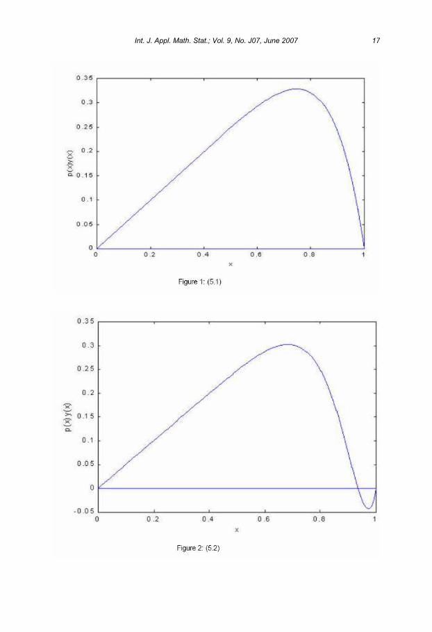
Example 2. The Latzko equation: It has the form
− 1x7
(py′)′ + y = λy; 0 < x < 1
with p(x) =(1 − x7
). This is a historical differential equation associated with a heat conduction
problem studied for the first time by Latzko in 1920. For details on the problem see Fichera [9].
The endpoint 0 is clearly regular while the endpoint 1 is singular since 10(1− x7)−1dx = ∞. For
boundary conditions we can take
θ(x) = 1 and φ(x) = ln(1
x − 1), I = (0, 1).
This means the boundary conditions are
y(0) = 0; W (y, ψ)(1−) = 0.
We solve the above singular boundary value problem for the eigenvalues λ using Algorithm 1.
n λ−iterative λ−SLEIGN2 λ−Durfee W (y, ψ)(1−)
0 8.727820 8.7274702 8.72747 3.634088-8
1 152.4451 152.423014 152.423 6.131883-7
2 435.1673 435.060768 435.060 -3.656848-7
3 855.9708 855.681700 855.680 -9.60201-7
Again the computed values were done with a step size h = 116 and the initial value problems
were solved using Runge-Kutta of order 4. The solutions corresponding to the first two eigen-
values are shown in figures 5.1 and 5.2.
ftbpF5.5677in3.3261in0infig1.gifftbpF5.8297in3.7455in0infig2.gif
References
[1] Agamaliyeva, A., and Nabiyevb, A., On Eigenvalues of Some Boundary Value Problems
for a Polynomial Pencil of Sturm–Liouville Equation, Appl. Math. and Comput., 165(2005),
503-515.
16 International Journal of Applied Mathematics & Statistics
Int. J. Appl. Math. Stat.; Vol. 9, No. J07, June 2007 17
References:
[1] Agamaliyeva, A., and Nabiyevb, A., On Eigenvalues of Some Boundary Value Problems for a Polynomial Pencil of Sturm–Liouville Equation, Appl. Math. and Comput., 165(2005), 503-515.
[2] Ascher, U. M., Matthheij, R. M., Russell, R. D. Numerical Solution Of Boundary Value Problems for Ordinary Differential Equations, Classics In Applied Mathematics, 13, 1995.
[3] Attili, B.S., Elgindi, M.B., Elgebeily, M.A. ”Initial Value Methods for the Eigenelements of Singular Two-Point Boundary Value Problems”, AJSE, 22 No.2C (1997), pp 67-77.
[4] Bailey, P. B., Everitt, W. N. and Zettl, A., Algorithm 810: The SLEIGN2 Sturm-Liouville Code - ACM Transactions on Mathematical Software (TOMS) archive, 27(2001), 143 -192.
[5] Bailey, P. B., Garbow, B. S., Kaper, G. H. and Zettl, A., Eigenvalue and Eigenfunction Computation of Sturm-Liouville Problems, ACM Trans. Math. Software, 17 (1991), 491-499.
[6] Ciarlet, P.G., Schultz, M.H., Varga, R.S., Numerical Methods of High-Order Accuracy for Nonlinear Boundary Vale Problems. I. One Dimensional Problem, Numer. Math., 9(1967), 394-430.
[7] Chu, Ch., Some Comparison Theorems for Sturm–Liouville Eigenvalue Problems*1, J. Math. Anal. Appl., 262(2001), 376-387.
[8] El-Gebeily, M. A. and Attili, B. S., An Iterative Shooting Method for a Certain Class of Singular Two-Point Boundary Value Problems, Comput. Math. Applic., 45(2003), 69-76.
[9] Fichera, G., Numerical and Quantitative Analysis (Pitman, London: 1978).
[10] Hassi, S., M650ller, M., and De Snoo, H., Singular Sturm–Liouville Problems Whose Coefficients Depend Rationally on the Eigenvalue Parameter, J. of Math. Anal. Appl., 295(2004), 258-275.
[11] Kong, Q., Moller, M., Wu, H. and Zettl, A., Indefinite Sturm–Liouville Problems, Proc. Roy. Soc. Edinburgh Sect. A 133 (2003), 639–652.
[12] Kong, Q., Wu, H. and Zettl, A., Singular Left-Definite Sturm–Liouville Problems, J. Diff. Equ., 206(2004), 1-29.
[13] Mukhtarov, O. Sh., Kadakal, M. and Muhtarov, F. S., Eigenvalues and Normalized Eigenfunctions of Discontinuous Sturm-Liouville Problem with Transmission Conditions, Rep. Math. Phys., 54(2004), 41-56.
[14] M. A. Naimark, Linear Differential Operators, Part II, Ungar, New York, 1968.
[15] Reid, W. T., Sturmian Theory for Ordinary Differential Equations, Springer Verlag, New York, 1980.
[16] Zettl, A., ”Sturm-Liouville Problems”, in ”Spectral Theory and Computational Methods of Sturm-Liouville Problems”, Don Hinton, Philip Schaefer, Ed, Lecture Notes in Pure and Applied Mathematics, 191, Marcel Dekker, Inc. 1997.
[17] Zettl, A., Sturm–Liouville problems, Spectral Theory and Computational Methods of Sturm–Liouville Problems (Knoxville, TN, 1996), Lecture Notes in Pure and Applied Mathematics, 191, Dekker, New York, 1997, 1–104.
18 International Journal of Applied Mathematics & Statistics
Euler-type Boundary Value Problems in Quantum Calculus
Martin Bohner1 and Thomas Hudson2 ∗
University of Missouri–Rolla, Rolla, MO 65401, [email protected] and [email protected] of Mathematics and Statistics
2Department of Mechanical and Aerospace Engineering
ABSTRACT
We study a boundary value problem consisting of a second-order q-difference equation to-
gether with Dirichlet boundary conditions. Separation of variables leads us to an eigenvalue
problem for a second-order Euler q-difference equation. We determine the exact number of
eigenvalues.
Keywords: Euler–Cauchy dynamic equation, quantum calculus.
2000 Mathematics Subject Classification: 39A13, 34K10, 65N25.
1 Introduction
While in ordinary calculus we study differential equations and in discrete calculus we study
difference equations, we study so-called q-difference equations in quantum calculus. Let
q > 1 and T = qk : k ∈ N0. (1.1)
For a function u : T × T → R, we define the Jackson derivatives of u with respect to the first
and the second variable, respectively, by
ux(x, t) =u(qx, t) − u(x, t)
(q − 1)xand ut(x, t) =
u(x, qt) − u(x, t)(q − 1)t
.
Let N ∈ N. In this paper, we consider the boundary value problem
x2uxx = t2utt, u(1, t) = u(qN , t) = 0, (1.2)
which is a second-order q-difference equation together with Dirichlet boundary conditions. For
material on quantum calculus we refer to the monograph by Kac and Cheung (Kac and Cheung
2002), the paper by Bohner and Unal (Bohner and Unal 2005), and the books about dynamic
equations on time scales by Bohner and Peterson (Bohner and Peterson 2001, Bohner and
Peterson 2003).∗Research supported by UMR’s OURE program
International Journal of Applied Mathematics & Statistics,ISSN 0973-1377 (Print), ISSN 0973-7545 (Online)Copyright © 2007 by IJAMAS, CESER IJAMAS: June 2007, Vol. 9, No. J07, 19-23
Now we rewrite the second-order q-difference equation in (1.2) as a second-order q-recursion
relation. By the definition of the Jackson derivative, the second-order partial of u with respect
to x is given by
uxx(x, t) =ux(qx, t) − ux(x, t)
(q − 1)x. (1.3)
When we expand equation (1.3), we obtain
uxx(x, t) =u(q2x,t)−u(qx,t)
(q−1)qx − u(qx,t)−u(x,t)(q−1)x
(q − 1)x.
Similarly we can compute the partial utt. Thus, the second-order q-difference equation in (1.2)
is equivalent to
x2
(u(q2x, t) − (q + 1)u(qx, t) + qu(x, t)
x2
)= t2
(u(x, q2t) − (q + 1)u(x, qt) + qu(x, t)
t2
),
i.e.,
u(q2x, t) − (q + 1)u(qx, t) + qu(x, t) = u(x, q2t) − (q + 1)u(x, qt) + qu(x, t). (1.4)
The setup of this paper is as follows. In the next section, we use separation of variables to
arrive at a certain eigenvalue problem. Finally, in Section 3 we determine the eigenvalues and
the number of eigenvalues of the resulting eigenvalue problem. An example is given as well.
2 Separation of Variables
We let u(x, t) = f(x)g(t) so that u(qx, t) = f(qx)g(t) and u(q2x, t) = f(q2x)g(t). This is also
applied to the terms u(x, qt) and u(x, q2t). When we substitute these values into the partial
q-difference equation (1.4), we get
f(q2x)g(t) − (q + 1)f(qx)g(t) + qf(x)g(t) = f(x)g(q2t) − (q + 1)f(x)g(qt) + qf(x)g(t). (2.1)
Now we divide each side of (2.1) by f(x)g(t) to gather like terms and then set both sides equal
to a constant λ to arrive at
f(q2x) − (q + 1)f(qx) + qf(x)f(x)
=g(q2t) − (q + 1)g(qt) + qg(t)
g(t)= λ. (2.2)
Hence, from (1.2) and (2.2), the eigenvalue problem for f is
f(q2x) − (q + 1)f(qx) + (q − λ)f(x) = 0, f(1) = f(qN ) = 0. (2.3)
The second-order q-difference equation in (2.3) is an Euler–Cauchy q-difference equation as
studied in (Bohner and Unal 2005). We let f(x) = αlogq x, which in return gives us
f(qx) = αlogq qx = αf(x) and f(q2x) = f(q(qx)) = αf(qx) = α2f(x).
Now we make these substitutions into the Euler–Cauchy equation in (2.3) and get
α2f(x) − (q + 1)αf(x) + (q − λ)f(x) = 0.
20 International Journal of Applied Mathematics & Statistics

The characteristic equation therefore reads
α2 − (q + 1)α + (q − λ) = 0. (2.4)
We solve (2.4) for α and get
α =q + 1 ±√(q + 1)2 − 4(q − λ)
2=
q + 12
±√(
q − 12
)2
+ λ.
Hence we let
α1 =q + 1
2+
√(q − 1
2
)2
+ λ and α2 =q + 1
2−√(
q − 12
)2
+ λ.
We distinguish the following three cases:
Case I. λ > −(
q − 12
)2
;
Case II. λ = −(
q − 12
)2
;
Case III. λ < −(
q − 12
)2
.
The general solution of the Euler–Cauchy equation in (2.3) for each case is found in (Bohner
and Unal 2005) as follows:
Case I: f(x) = c1αlogq x
1 + c2αlogq x
2 , (2.5)
Case II: f(x) = (c1 lnx + c2)(
q + 12
)logq x
, (2.6)
Case III: f(x) = |α|logq x(c1 cos (θ logq x) + c2 sin (θ logq x)), (2.7)
where θ = arccos(
Re α|α|)
and c1, c2 ∈ R.
3 Finding Eigenvalues
Our next step is to look at the three different cases and thus find the eigenvalues of (2.3).
Case I
We apply the first Dirichlet condition f(1) = 0 to (2.5) to obtain
f(1) = c1αlogq 1
1 + c2αlogq 1
2 = c1 + c2 = 0 so that c := c1 = −c2.
Now we use the relationship between c1 and c2 and apply it to the general solution and then
use the other Dirichlet condition f(qN ) = 0 to find
0 = f(qN ) = c
(α
logq qN
1 − αlogq qN
2
)= c
(αN
1 − αN2
).
Int. J. Appl. Math. Stat.; Vol. 9, No. J07, June 2007 21

Since c = 0 results in the trivial solution, we shall discuss
αN1 = αN
2 .
This can occur if α1 = α2 or (for even N ) if α1 = −α2. First, α1 = α2 implies
q + 12
+
√(q − 1
2
)2
+ λ =q + 1
2−√(
q − 12
)2
+ λ,
i.e.,
2
√(q − 1
2
)2
+ λ = 0 so that λ = −(
q − 12
)2
,
which is not a valid value for λ in Case I. Next, α1 = −α2 implies
q + 12
+
√(q − 1
2
)2
+ λ = −q + 12
+
√(q − 1
2
)2
+ λ
which results in q = −1, contradicting (1.1). Thus there are no eigenvalues in this case.
Case II
Now we look at the case where λ = −( q−12 )2 and use equation (2.6) with the first Dirichlet
condition to find
0 = f(1) = (c1 ln 1 + c2)(
q + 12
)logq 1
= c2.
We let c := c1 and apply the second Dirichlet condition, which gives
0 = f(qN ) = c ln qN
(q + 1
2
)logq qN
= cN ln q
(q + 1
2
)N
.
For this to be true either c = 0, N = 0, q = 1, or q = −1, which would all not lead to any
eigenvalues. Hence there are no eigenvalues in this case also.
Case III
Finally we look at the case where λ < −( q−12 )2 and use equation (2.7) with the first Dirichlet
condition to find
0 = f(1) = |α|logq 1(c1 cos(θ logq 1) + c2 sin(θ logq 1)) = c1.
We let c := c2 and apply the other Dirichlet condition to obtain
0 = f(qN ) = |α|logq qN(c sin(θ logq qN )) = c|α|N sin(θN). (3.1)
Note now that
|α| =√
q − λ and θ = arccos(
Re α
|α|)
= arccos(
q + 12√
q − λ
).
Therefore we obtain from (3.1) that
0 = f(qN ) = c√
q − λN
sin(θN). (3.2)
22 International Journal of Applied Mathematics & Statistics
When looking at (3.2), we can see that λ = q would work, but this is not in the range of values
we are looking at for this case. So we consider the only other possible solution, which is
sin(θN) = 0. This leads us to θmN = mπ, which gives us the values λm, m ∈ N0, where
arccos(
q + 12√
q − λm
)=
mπ
N. (3.3)
Solving for λm provides
λm = q −(
q + 12 cos (mπ
N )
)2
(3.4)
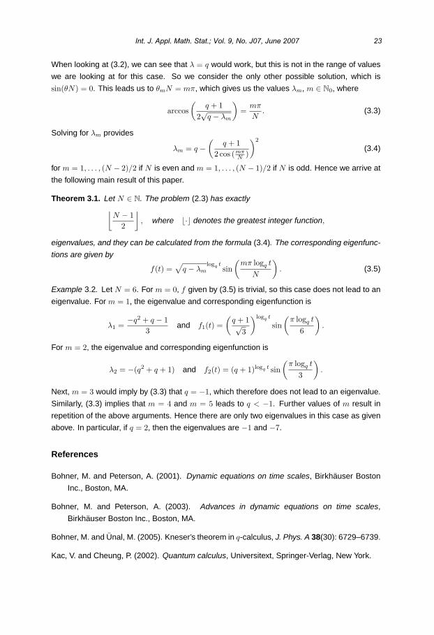
for m = 1, . . . , (N − 2)/2 if N is even and m = 1, . . . , (N − 1)/2 if N is odd. Hence we arrive at
the following main result of this paper.
Theorem 3.1. Let N ∈ N. The problem (2.3) has exactly⌊N − 1
2
⌋, where · denotes the greatest integer function,
eigenvalues, and they can be calculated from the formula (3.4). The corresponding eigenfunc-
tions are given by
f(t) =√
q − λmlogq t
sin(
mπ logq t
N
). (3.5)
Example 3.2. Let N = 6. For m = 0, f given by (3.5) is trivial, so this case does not lead to an
eigenvalue. For m = 1, the eigenvalue and corresponding eigenfunction is
λ1 =−q2 + q − 1
3and f1(t) =
(q + 1√
3
)logq t
sin(
π logq t
6
).
For m = 2, the eigenvalue and corresponding eigenfunction is
λ2 = −(q2 + q + 1) and f2(t) = (q + 1)logq t sin(
π logq t
3
).
Next, m = 3 would imply by (3.3) that q = −1, which therefore does not lead to an eigenvalue.
Similarly, (3.3) implies that m = 4 and m = 5 leads to q < −1. Further values of m result in
repetition of the above arguments. Hence there are only two eigenvalues in this case as given
above. In particular, if q = 2, then the eigenvalues are −1 and −7.
References
Bohner, M. and Peterson, A. (2001). Dynamic equations on time scales, Birkhauser Boston
Inc., Boston, MA.
Bohner, M. and Peterson, A. (2003). Advances in dynamic equations on time scales,
Birkhauser Boston Inc., Boston, MA.
Bohner, M. and Unal, M. (2005). Kneser’s theorem in q-calculus, J. Phys. A 38(30): 6729–6739.
Kac, V. and Cheung, P. (2002). Quantum calculus, Universitext, Springer-Verlag, New York.
Int. J. Appl. Math. Stat.; Vol. 9, No. J07, June 2007 23
Positive Solutions of Third Order Boundary Value Problems
Abdelkader Boucherif
Differential Equations Research Lab.Department of Mathematical Sciences
King Fahd University of Petroleum and MineralsBox 5046, Dhahran, 31261, Saudi Arabia
e-mail: [email protected]
ABSTRACT
We investigate the existence of positive solutions of third order boundary value problems
with changing sign Caratheodory nonlinearities of the form. We provide simple sufficient
conditions on the nonlinearity f in order to obtain a priori bounds on solutions of a one-
parameter family of problems, related to the original one. We then rely on the topological
transversality theorem to prove the existence of positive solutions of the given problem. As
a byproduct, we shall obtain a multiplicity result.
Keywords: Third order differential equations, three-point boundary value problems, a priori
bound on solutions, positive solutions, Granas topological transversality theorem.
2000 Mathematics Subject Classification: 34B15, 34B18.
1 Introduction
In this paper, we are concerned with the existence of positive solutions of three-point boundary
value problems for third order differential equations,
u′′′(t) = f(t, u(t), u′(t), u′′(t)) 0 < t < 1 (1)
u(0) = u′(a) = u(1) = 0, 0 < a < 1. (2)
Problems of this type arise naturally in the description of physical phenomena, where only
positive solutions, i.e. solutions u satisfying u(t) > 0 for all t ∈ (0, 1), are meaningful. It is well
known that Krasnoselskii’s fixed point theorem in a cone (see [14],) has been instrumental in
proving existence of positive solutions of problem (1), (2).
In the last decade or so, several papers have been devoted to the study of positive solutions to
third order differential equations with two-point or three-point boundary conditions. Most of the
previous works assume that f is nonnegative, depends only on u, and some other conditions.
See for instance[1], [3], [4], [5],[8], [9], [12], [14], [15] and [16]. It should be pointed out that
even in the case of second order boundary problems, only few papers have dealt with changing
International Journal of Applied Mathematics & Statistics,ISSN 0973-1377 (Print), ISSN 0973-7545 (Online)Copyright © 2007 by IJAMAS, CESER IJAMAS: June 2007, Vol. 9, No. J07, 24-34

sign nonlinearities, that also depend on the first derivative of u. We refer the interested reader
to [2] and [6].
Our aim, in this paper, is to establish sufficient conditions on the nonlinearity f that will allow
us to obtain a priori bounds on solutions of a one-parameter family of problems related to (1),
(2). We, then, rely on the topological transversality theorem of Granas (see [10] for definitions
and details) to prove the existence of at least one positive solution of problem (1), (2).
Our assumptions are simple and more general than the conditions found in the literature. In
fact, we obtain a multiplicity result as a byproduct of our main result, with no extra assumptions.
We exploit the fact that the nonlinearity changes sign with respect to its second argument. We
do not rely on cone preserving mappings, and the sign of the Green’s function, see see [4],
of the corresponding linear homogeneous problem plays no role in our analysis. We assume,
however, the existence of positive upper and lower solutions. For general results, not neces-
sarily on positive solutions, see [7], [9] and [11].
2 Preliminaries
Let I denote the real interval [0, 1]. AC(I) is the Banach space of real-valued absolutely
continuous functions on I, equipped with the norm ||u||0 := max|u(t)|; t ∈ I. For k =1, 2, . . . ACk(I) is the Banach space of absolutely continuous functions defined on I together
with their derivatives up to order k, with the norm ||u||(k) = ‖u‖0 + ‖u′‖0 + . . .+ ‖u(k)‖0. AC20 (I)
is the space of functions u ∈ AC2(I) satisfying u(0) = u′(a) = u(1) = 0; L1(I) is the space
of Lebesgue integrable functions on I with its usual norm.
We say that f : I × R3 → R is a Caratheodory function, if f satisfies the following conditions
(i) f(t, ., ., .) is continuous for almost every t ∈ I,
(ii) f(., u, v, w) is measurable for all (u, v, w) ∈ R3,
(iii) for every R > 0, there exists hR ∈ L1(I) such that |u| +|v|+|w| ≤ R implies |f(t, u, v, w)| ≤hR(t) for almost all t ∈ I.
Since our arguments are based on the topological transversality theorem we consider the
following one-parameter family of problems
u′′′(t) = λ f(t, u(t), u′(t), u′′(t)) 0 < t < 1 (3)
u(0) = u′(a) = u(1) = 0, 0 < a < 1 (4)
for 0 ≤ λ ≤ 1.
For λ = 0 problem (3), (4) has only the trivial solution.
Proof. Obvious.
It follows that the corresponding Green’s function G(t, s) exists. To construct G(t, s) we proceed
as follows (for a general nth order problem see [13] ). Let uj(t), 1 ≤ j ≤ 3 be solutions of y′′′ = 0
Int. J. Appl. Math. Stat.; Vol. 9, No. J07, June 2007 25

such that the following boundary conditions are satisfied
u1(0) = 1, u′1(a) = 0, u1(1) = 0
u2(0) = 0, u′2(a) = 1, u2(1) = 0
u3(0) = 0, u′3(a) = 0, u3(1) = 1.
Simple computations give
u1(t) = 1 − t2 − 2at
1 − 2a, u2(t) =
−t2 + t
1 − 2a, u3(t) =
t2 − 2at
1 − 2a.
On the other hand consider the function v(t, s) :=(t − s)2
2. Then
∂3v
∂t3= 0.
Let v1(s) := v(0, s), v2(s) := v(a, s) and v3(s) := v(1, s), so that
v1(s) =s2
2, v2(s) =
(a − s)2
2, v3(s) =
(1 − s)2
2.
Now, let ϕ(t, s) = u1(t)v1(s) + u2(t)v2(s) + u3(t)v3(s). One can easily show that ϕ(., s) is a
solution of y′′′ = 0, for each fixed s. Moreover ϕ(0, s) = v(0, s), ϕ′(a, s) = v(a, s) and ϕ(1, s) =v(1, s). It follows from the uniqueness of solutions of a linear homogeneous boundary value
problem that ϕ(t, s) = v(t, s), that is
u1(t)v1(s) + u2(t)v2(s) + u3(t)v3(s) =(t − s)2
2, ∀ (t, s) ∈ I2.
We define G(t, s) as follows.
For 0 ≤ s ≤ a, we let
G(t, s) =
⎧⎪⎨⎪⎩−u2(t)v2(s) − u3(t)v3(s) 0 ≤ t ≤ s
u1(t)v1(s) s ≤ t ≤ a
and for a ≤ s ≤ 1, we let
G(t, s) =
⎧⎪⎨⎪⎩−u3(t)v3(s) a ≤ t ≤ s
u1(t)v1(s) + u2(t)v2(s) s ≤ t ≤ 1.
If f : I × R3 → R is a Caratheodory function, then u ∈ A C2(I) is a solution of (3), (4) if and
only if u is a solution of the integral equation
u(t) = λ
∫ 1
0G(t, s)f(s, u(s), u′(s), u′′(s))ds. (5)
Assume that f : I × R3 → R is a Caratheodory function. Then, the operator T : AC20 → AC2
0 ,
defined by Tu(t) =∫ 10 G(t, s)f(s, u(s), u′(s), u′′(s))ds, is continuous and completely continu-
ous.
Proof. (i) T is continuous. For, let un → u in AC20 (I). Then, for k = 0, 1, 2, u
(k)n → u(k) uniformly
on I. Given that f is continuous with respect to its second, third and fourth arguments, and for
26 International Journal of Applied Mathematics & Statistics

k = 0, 1,∂k
∂tkG(., .) is uniformly continuous on I × I, and also
∂2
∂t2G(., .) is continuous on I × I
except on the set (t, t); t ∈ I, which has measure zero, we have
∂k
∂tkG(t, s)f(s, un(s), u′
n(s), u′′n(s)) → ∂k
∂tkG(t, s)f(s, u(s), u′(s), u′′(s)), as n → +∞,
for almost every s ∈ I, and k = 0, 1, 2. Now, there exists M > 0, independent of n ∈ N, such
that |un|+ |u′n|+ |u′′
n| ≤ M for all n ∈ N. Hence, there is hM ∈ L1(I) such that for all n ∈ N, we
have ∣∣f(s, un(s), u′n(s), u′′
n(s))∣∣ ≤ hM (s) for almost all s ∈ I.
The Lebesgue dominated convergence theorem implies that, as n → +∞∫ 1
0
∂k
∂tkG(t, s)f(s, un(s), u′
n(s), u′′n(s))ds →
∫ 1
0
∂k
∂tkG(t, s)f(s, u(s), u′(s), u′′(s))ds.
This shows that for k = 0, 1, 2, and all t ∈ I
(Tun)(k) (t) → (Tu)(k) (t) as n → +∞.
Therefore
‖Tun‖(2) → ‖Tu‖(2) as n → +∞.
(ii) T is completely continuous. For, let B = B(0, r) be a ball in AC20 (I), and let u ∈ B. Then
‖u‖(2) ≤ r.
Since f is a Caratheodory function there exits hr ∈ L1(I) such that∣∣f(t, u(t), u′(t), u′′(t))∣∣ ≤ hr(t) for almost all t ∈ I.
Thus
‖Tu‖(2) ≤ max|G(t, s)| +∣∣∣∣ ∂
∂tG(t, s)
∣∣∣∣+ ∣∣∣∣ ∂2
∂t2G(t, s)
∣∣∣∣ ; (t, s) ∈ I2 ‖hr‖L1 .
This shows that T (B) is uniformly bounded. To show that T (B) is equicontinuous, let u ∈ B
and 0 < t1 < t2 < 1. Then
Tu(t2) − Tu(t1) =∫ 1
0[G(t2, s) − G(t1, s)]f(s, u(s), u′(s), u′′(s))ds
so that
|Tu(t2) − Tu(t1)| ≤∫ 1
0|G(t2, s) − G(t1, s)|hr(s)ds
≤ maxs∈I
|G(t2, s) − G(t1, s)| ‖hr‖L1 .
Since G(., .) is uniformly continuous on I × I, it follows that |Tu(t2) − Tu(t1)| → 0 whenever
|t2 − t1| → 0. The conclusion follows from Arzela-Ascoli’s theorem.
Int. J. Appl. Math. Stat.; Vol. 9, No. J07, June 2007 27
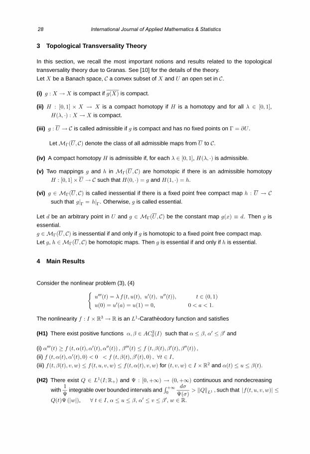
3 Topological Transversality Theory
In this section, we recall the most important notions and results related to the topological
transversality theory due to Granas. See [10] for the details of the theory.
Let X be a Banach space, C a convex subset of X and U an open set in C.
(i) g : X → X is compact if g(X) is compact.
(ii) H : [0, 1] × X → X is a compact homotopy if H is a homotopy and for all λ ∈ [0, 1],H(λ, ·) : X → X is compact.
(iii) g : U → C is called admissible if g is compact and has no fixed points on Γ = ∂U .
Let MΓ(U, C) denote the class of all admissible maps from U to C.
(iv) A compact homotopy H is admissible if, for each λ ∈ [0, 1], H(λ, ·) is admissible.
(v) Two mappings g and h in MΓ(U, C) are homotopic if there is an admissible homotopy
H : [0, 1] × U → C such that H(0, ·) = g and H(1, ·) = h.
(vi) g ∈ MΓ(U, C) is called inessential if there is a fixed point free compact map h : U → Csuch that g|Γ = h|Γ. Otherwise, g is called essential.
Let d be an arbitrary point in U and g ∈ MΓ(U, C) be the constant map g(x) ≡ d. Then g is
essential.
g ∈ MΓ(U, C) is inessential if and only if g is homotopic to a fixed point free compact map.
Let g, h ∈ MΓ(U, C) be homotopic maps. Then g is essential if and only if h is essential.
4 Main Results
Consider the nonlinear problem (3), (4)u′′′(t) = λ f(t, u(t), u′(t), u′′(t)), t ∈ (0, 1)u(0) = u′(a) = u(1) = 0, 0 < a < 1.
The nonlinearity f : I × R3 → R is an L1-Caratheodory function and satisfies
(H1) There exist positive functions α, β ∈ AC20 (I) such that α ≤ β, α′ ≤ β′ and
(i) α′′′(t) ≥ f (t, α(t), α′(t), α′′(t)) , β′′′(t) ≤ f (t, β(t), β′(t), β′′(t)) ,
(ii) f (t, α(t), α′(t), 0) < 0 < f (t, β(t), β′(t), 0) , ∀t ∈ I,
(iii) f(t, β(t), v, w) ≤ f(t, u, v, w) ≤ f(t, α(t), v, w) for (t, v, w) ∈ I × R2 and α(t) ≤ u ≤ β(t).
(H2) There exist Q ∈ L1(I; R+) and Ψ : [0, +∞) → (0, +∞) continuous and nondecreasing
with1Ψ
integrable over bounded intervals and∫ +∞0
dσ
Ψ(σ)> ‖Q‖L1 , such that |f(t, u, v, w)| ≤
Q(t)Ψ (|w|), ∀ t ∈ I, α ≤ u ≤ β, α′ ≤ v ≤ β′, w ∈ R.
28 International Journal of Applied Mathematics & Statistics
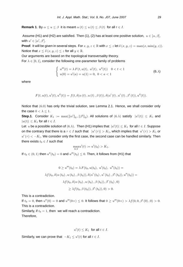
Remark 1. By α ≤ u ≤ β it is meant α (t) ≤ u (t) ≤ β (t) for all t ∈ I.
Assume (H1) and (H2) are satisfied. Then (1), (2) has at least one positive solution, u ∈ [α, β],with u′ ∈ [α′, β′].Proof. It will be given in several steps. For x, y, z ∈ R with x ≤ z let δ (x, y, z) = max(x,min(y, z)).Notice that x ≤ δ (x, y, z) ≤ z for all y ∈ R.
Our arguments are based on the topological transversality theory.
For λ ∈ [0, 1], consider the following one-parameter family of problemsu′′′(t) = λ F (t, u(t), u′(t), u′′(t)) 0 < t < 1u(0) = u′(a) = u(1) = 0, 0 < a < 1
(6.λ)
where
F (t, u(t), u′(t), u′′(t)) = f(t, δ(α (t) , u (t) , β (t)), δ(α′ (t) , u′ (t) , β′ (t)), u′′(t)).
Notice that (6.0) has only the trivial solution, see Lemma 2.1. Hence, we shall consider only
the case 0 < λ ≤ 1.
Step.1. Consider K1 := max(‖α′‖0 , ‖β′‖0). All solutions of (6.λ) satisfy |u′(t)| ≤ K1 and
|u(t)| ≤ K1 for all t ∈ I.
Let u be a possible solution of (6.λ). Then (H1) implies that |u′(t)| ≤ K1 for all t ∈ I. Suppose
on the contrary that there is a τ ∈ I such that |u′ (τ)| > K1, which implies that u′ (τ) > K1 or
u′ (τ) < −K1. We consider only the first case, the second case can be handled similarly. Then
there exists t0 ∈ I such that
maxt∈I
u′(t) := u′(t0) > K1.
If t0 ∈ (0, 1) then u′′(t0) = 0 and u′′′(t0) ≤ 0. Then, it follows from (H1) that
0 ≥ u′′′(t0) = λ F (t0, u(t0), u′(t0), u′′(t0)) =
λf(t0, δ(α (t0) , u (t0) , β (t0)), δ(α′ (t0) , u′ (t0) , β′ (t0)), u′′(t0)) =
λf(t0, δ(α (t0) , u (t0) , β (t0)), β′ (t0) , 0)
≥ λf(t0, β (t0)), β′ (t0)), 0) > 0.
This is a contradiction.
If t0 = 0, then u′′(0) = 0 and u′′′(0+) ≤ 0. It follows that 0 ≥ u′′′(0+) > λf(0, 0, β′ (0) , 0) > 0.
This is a contradiction.
Similarly, if t0 = 1, then we will reach a contradiction.
Therefore,
u′(t) ≤ K1 for all t ∈ I.
Similarly, we can prove that −K1 ≤ u′(t) for all t ∈ I.
Int. J. Appl. Math. Stat.; Vol. 9, No. J07, June 2007 29
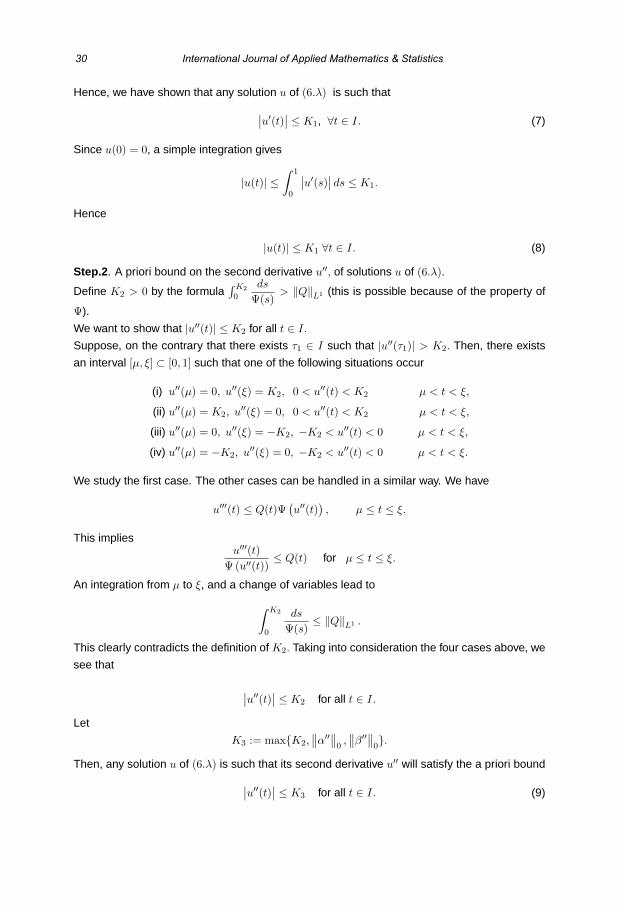
Hence, we have shown that any solution u of (6.λ) is such that∣∣u′(t)∣∣ ≤ K1, ∀t ∈ I. (7)
Since u(0) = 0, a simple integration gives
|u(t)| ≤∫ 1
0
∣∣u′(s)∣∣ ds ≤ K1.
Hence
|u(t)| ≤ K1 ∀t ∈ I. (8)
Step.2. A priori bound on the second derivative u′′, of solutions u of (6.λ).
Define K2 > 0 by the formula∫K2
0
ds
Ψ(s)> ‖Q‖L1 (this is possible because of the property of
Ψ).
We want to show that |u′′(t)| ≤ K2 for all t ∈ I.
Suppose, on the contrary that there exists τ1 ∈ I such that |u′′(τ1)| > K2. Then, there exists
an interval [µ, ξ] ⊂ [0, 1] such that one of the following situations occur
(i) u′′(µ) = 0, u′′(ξ) = K2, 0 < u′′(t) < K2 µ < t < ξ,
(ii) u′′(µ) = K2, u′′(ξ) = 0, 0 < u′′(t) < K2 µ < t < ξ,
(iii) u′′(µ) = 0, u′′(ξ) = −K2, −K2 < u′′(t) < 0 µ < t < ξ,
(iv) u′′(µ) = −K2, u′′(ξ) = 0, −K2 < u′′(t) < 0 µ < t < ξ.
We study the first case. The other cases can be handled in a similar way. We have
u′′′(t) ≤ Q(t)Ψ(u′′(t)
), µ ≤ t ≤ ξ.
This impliesu′′′(t)
Ψ (u′′(t))≤ Q(t) for µ ≤ t ≤ ξ.
An integration from µ to ξ, and a change of variables lead to∫ K2
0
ds
Ψ(s)≤ ‖Q‖L1 .
This clearly contradicts the definition of K2. Taking into consideration the four cases above, we
see that
∣∣u′′(t)∣∣ ≤ K2 for all t ∈ I.
Let
K3 := maxK2,∥∥α′′∥∥
0,∥∥β′′∥∥
0.
Then, any solution u of (6.λ) is such that its second derivative u′′ will satisfy the a priori bound∣∣u′′(t)∣∣ ≤ K3 for all t ∈ I. (9)
30 International Journal of Applied Mathematics & Statistics
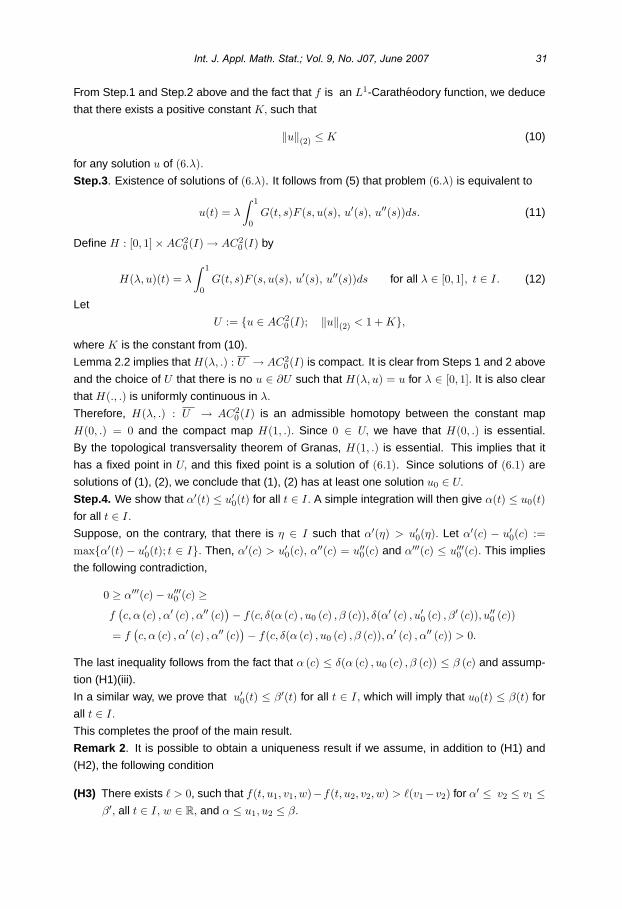
From Step.1 and Step.2 above and the fact that f is an L1-Caratheodory function, we deduce
that there exists a positive constant K, such that
‖u‖(2) ≤ K (10)
for any solution u of (6.λ).Step.3. Existence of solutions of (6.λ). It follows from (5) that problem (6.λ) is equivalent to
u(t) = λ
∫ 1
0G(t, s)F (s, u(s), u′(s), u′′(s))ds. (11)
Define H : [0, 1] × AC20 (I) → AC2
0 (I) by
H(λ, u)(t) = λ
∫ 1
0G(t, s)F (s, u(s), u′(s), u′′(s))ds for all λ ∈ [0, 1], t ∈ I. (12)
Let
U := u ∈ AC20 (I); ‖u‖(2) < 1 + K,
where K is the constant from (10).
Lemma 2.2 implies that H(λ, .) : U → AC20 (I) is compact. It is clear from Steps 1 and 2 above
and the choice of U that there is no u ∈ ∂U such that H(λ, u) = u for λ ∈ [0, 1]. It is also clear
that H(., .) is uniformly continuous in λ.
Therefore, H(λ, .) : U → AC20 (I) is an admissible homotopy between the constant map
H(0, .) = 0 and the compact map H(1, .). Since 0 ∈ U, we have that H(0, .) is essential.
By the topological transversality theorem of Granas, H(1, .) is essential. This implies that it
has a fixed point in U, and this fixed point is a solution of (6.1). Since solutions of (6.1) are
solutions of (1), (2), we conclude that (1), (2) has at least one solution u0 ∈ U.
Step.4. We show that α′(t) ≤ u′0(t) for all t ∈ I. A simple integration will then give α(t) ≤ u0(t)
for all t ∈ I.
Suppose, on the contrary, that there is η ∈ I such that α′(η) > u′0(η). Let α′(c) − u′
0(c) :=maxα′(t) − u′
0(t); t ∈ I. Then, α′(c) > u′0(c), α′′(c) = u′′
0(c) and α′′′(c) ≤ u′′′0 (c). This implies
the following contradiction,
0 ≥ α′′′(c) − u′′′0 (c) ≥
f(c, α (c) , α′ (c) , α′′ (c)
)− f(c, δ(α (c) , u0 (c) , β (c)), δ(α′ (c) , u′0 (c) , β′ (c)), u′′
0 (c))
= f(c, α (c) , α′ (c) , α′′ (c)
)− f(c, δ(α (c) , u0 (c) , β (c)), α′ (c) , α′′ (c)) > 0.
The last inequality follows from the fact that α (c) ≤ δ(α (c) , u0 (c) , β (c)) ≤ β (c) and assump-
tion (H1)(iii).
In a similar way, we prove that u′0(t) ≤ β′(t) for all t ∈ I, which will imply that u0(t) ≤ β(t) for
all t ∈ I.
This completes the proof of the main result.
Remark 2. It is possible to obtain a uniqueness result if we assume, in addition to (H1) and
(H2), the following condition
(H3) There exists > 0, such that f(t, u1, v1, w)−f(t, u2, v2, w) > (v1−v2) for α′ ≤ v2 ≤ v1 ≤β′, all t ∈ I, w ∈ R, and α ≤ u1, u2 ≤ β.
Int. J. Appl. Math. Stat.; Vol. 9, No. J07, June 2007 31

Assume that the conditions (H1), (H2) and (H3) hold. Then Problem (1), (2) has a unique
positive solution u ∈ [α, β] with u′ ∈ [α′, β′].Proof. Theorem 4.1 guarantees the existence of at least one solution u ∈ [α, β] with u′ ∈[α′, β′].Suppose there are two solutions u1, u2 ∈ [α, β]. We exhibit that u′
1(t) = u′2(t) for all t ∈ I. A
simple integration will give u1(t) = u2(t) for all t ∈ I. Suppose on the contrary that u′1(ξ) = u′
2(ξ)for some ξ ∈ I. Let z(t) := u′
1(t) − u′2(t) for all t ∈ I. Suppose, first, that z(ξ) > 0. Let z(η) =
maxz(t); t ∈ I. Then, z(η) > 0, z′(η) = 0 and z′′(η) ≤ 0.
Since
z′′(t) = u′′′1 (t) − u′′′
2 (t) = f(t, u1(t), u′1(t), u
′′1(t)) − f(t, u2(t), u′
2(t), u′′2(t))
and
z′(η) = u′′1(η) − u′′
2(η) = 0
we have
0 ≥ z′′(η) = f(t, u1(η), u′1(η), u′′
1(η)) − f(t, u2(η), u′2(η), u′′
2(η)) =
= f(t, u1(η), u′1(η), u′′
1(η)) − f(t, u2(η), u′2(η), u′′
1(η)) > z (η) > 0.
This is a contradiction.
Similarly, if we assume z(ξ) < 0, we will arrive at a contradiction.
Therefore
u′1(t) = u′
2(t) for all t ∈ I.
This yields
u1(t) = u2(t) for all t ∈ I,
proving uniqueness.
5 Multiplicity of Solutions
In this section we use Theorem 4.1 to get multiplicity of solutions of problem (1), (2).
Assume f : I × R3 → R is a Caratheodory function and satisfies
(H4) there are sequences αj, βj of positive functions in AC20 (I) such that for all j = 1, 2, ...
(i) 0 ≤ αj ≤ βj ≤ αj+1, and α′j ≤ β′
j ≤ α′j+1,
(ii) α′′′j (t) ≥ f(t, αj (t) , α′
j (t) , α′′j (t)), β′′′
j (t) ≤ f(t, βj (t) , β′j (t) , β′′
j (t)),
(iii) f(t, αj (t) , α′j (t) , 0) < 0 < f(t, βj (t) , β′
j (t) , 0) , t ∈ I,
(iv) f(t, βj (t) , v, w) ≤ f(t, u, v, w) ≤ f(t, αj (t) , v, w) for (t, v, w) ∈ I × R2, αj(t) ≤ u ≤ βj(t),
(v) The condition (H2) holds on I × [ αj , βj ] × [α′j , β
′j ] × R.
Then, Problem (1), (2) has infinitely many positive solutions uj such that αj ≤ uj ≤ βj , and
α′j ≤ u′ ≤ β′
j .
32 International Journal of Applied Mathematics & Statistics
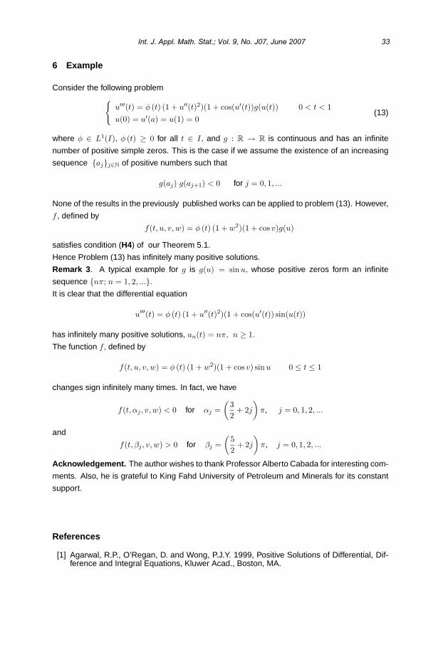
6 Example
Consider the following problemu′′′(t) = φ (t) (1 + u′′(t)2)(1 + cos(u′(t))g(u(t)) 0 < t < 1u(0) = u′(a) = u(1) = 0
(13)
where φ ∈ L1(I), φ (t) ≥ 0 for all t ∈ I, and g : R → R is continuous and has an infinite
number of positive simple zeros. This is the case if we assume the existence of an increasing
sequence ajj∈N of positive numbers such that
g(aj) g(aj+1) < 0 for j = 0, 1, ...
None of the results in the previously published works can be applied to problem (13). However,
f , defined by
f(t, u, v, w) = φ (t) (1 + w2)(1 + cos v)g(u)
satisfies condition (H4) of our Theorem 5.1.
Hence Problem (13) has infinitely many positive solutions.
Remark 3. A typical example for g is g(u) = sinu, whose positive zeros form an infinite
sequence nπ; n = 1, 2, ....It is clear that the differential equation
u′′′(t) = φ (t) (1 + u′′(t)2)(1 + cos(u′(t)) sin(u(t))
has infinitely many positive solutions, un(t) = nπ, n ≥ 1.
The function f, defined by
f(t, u, v, w) = φ (t) (1 + w2)(1 + cos v) sin u 0 ≤ t ≤ 1
changes sign infinitely many times. In fact, we have
f(t, αj , v, w) < 0 for αj =(
32
+ 2j
)π, j = 0, 1, 2, ...
and
f(t, βj , v, w) > 0 for βj =(
52
+ 2j
)π, j = 0, 1, 2, ...
Acknowledgement. The author wishes to thank Professor Alberto Cabada for interesting com-
ments. Also, he is grateful to King Fahd University of Petroleum and Minerals for its constant
support.
References
[1] Agarwal, R.P., O’Regan, D. and Wong, P.J.Y. 1999, Positive Solutions of Differential, Dif-ference and Integral Equations, Kluwer Acad., Boston, MA.
Int. J. Appl. Math. Stat.; Vol. 9, No. J07, June 2007 33
[2] Agarwal, R.P., O’Regan, D. and Stanek, S. 2003, Positive solutions of singular problemswith sign changing Caratheodory nonlinearities depending on x′, Journal of MathematicalAnalysis and Applications, 279 , 597-616.
[3] Anderson, D.R. 1998, Multiple positive solutions for a three-point boundary value problem,Math.Comput. Modeling 27, 49-57.
[4] Anderson, D.R. 2003, Green’s function for a third order generalized right focal problem,Journal of Mathematical Analysis and Applications, 288, 1-14.
[5] Boucherif, A. and Dahmane, M. 2000, Positive solutions of third order boundary valueproblems, Panamerican Mathematical Journal, 10, 79-103.
[6] Boucherif, A. and Henderson, J. 2005, Positive solutions of second order boundary valueproblems with changing sign Caratheodory nonlinearities, Submitted.
[7] Cabada, A., 1994, The method of upper and lower solutions for second, third, fourth andhigher order boundary value problems, Journal of Mathematical Analysis and Applica-tions, 185, 302-320.
[8] J. Chu, J. and Zhou, Z., 2006, Positive solutions for singular non-linear third order periodicboundary value problems, Nonlinear Analysis, 64, 1528-1542.
[9] Du, Z., Ge, W. and Lin, X. 2004, Existence of solutions for a class of third order nonlinearboundary value problems, Journal of Mathematical Analysis and Applications, 294, 104-112.
[10] Granas, A. and Dugundji, J. 2003, Fixed Point Theory, Springer Verlag, Berlin.
[11] Grossinho, M.R. and Minhos, F.M. 2001, Existence result for some third order separatedboundary value problems, Nonlinear Analysis 47, 2407-2418.
[12] Guo, D. and Lakshmikantham, V., 1988, Nonlinear Problems in Abstract Cones, AcademicPress, New York.
[13] Jackson, L.K. 1977, Boundary value problems for ordinary differential equations, in Hale,J. (Ed.), Studies in Differential Equations, The Mathematical Association of America, Vol.14, 93-127.
[14] Krasnoselskii, M.A. 1964, Positive Solutions of Operator Equations, Noordhoff, Holland.
[15] Sun, Y., 2005, Positive solutions of singular third order three-point boundary value prob-lem, Journal of Mathematical Analysis and Applications, 306, 589-603.
[16] Yang, Q. 2003, On the existence of positive solutions for nonlinear third order three-pointboundary value problem, Northeast Mathematical Journal, 19, 244-248.
34 International Journal of Applied Mathematics & Statistics

Controllability of Nondensely Defined Impulsive FunctionalSemilinear Differential Inclusions in Frechet Spaces
Johnny Henderson1 and Abdelghani Ouahab2
1Department of MathematicsBaylor University
Waco, TX 76798-7328 USAJohnny [email protected]
2Laboratoire de MathematiquesUniversite de Sidi Bel Abbes
BP 89, 22000 Sidi Bel Abbes, [email protected]
ABSTRACT
Frigon nonlinear alternative for multivalued admissible contractions in Frechet spaces, com-bined with integral semigroup theory, is used to investigate the controllability of someclasses of impulsive semilinear functional and neutral functional differential inclusions inFrechet spaces.
Key words and phrases: Impulsive functional differential inclusions, controllability, integralsolution, fixed point, Frechet space, admissible contraction.
AMS (MOS) Subject Classifications: 34G25, 34K25, 93B05
1 INTRODUCTION
This paper is concerned with an application of a recent Frigon nonlinear alternative, for admis-sible contraction maps in Frechet spaces (Frigon, 2002), to the existence of integral solutions offirst order controllability associated with impulsive semilinear functional and neutral functionaldifferential inclusions in Frechet spaces. In Section 3, we will consider first order controllabilityfor the impulsive semilinear functional differential inclusion,
y′(t) − Ay(t) ∈ F (t, yt) + (Bu)(t), a.e. t ∈ J := [0,∞) \ t1, t2, . . ., (1.1)
y(t+k ) − y(t−k ) = Ik(y(t−k )), k = 1, 2, . . . , (1.2)
International Journal of Applied Mathematics & Statistics,ISSN 0973-1377 (Print), ISSN 0973-7545 (Online)Copyright © 2007 by IJAMAS, CESER IJAMAS: June 2007, Vol. 9, No. J07, 35-54
y(t) = φ(t), t ∈ [−r, 0], (1.3)
where r > 0, F : J×D → P(E) is a multivalued map with compact values (P (E) is the family ofall nonempty subsets of E), A : D(A) ⊂ E → E is a nondensely defined closed linear operatoron E, B is a bounded linear operator from D(A) into D(A), D = ψ : [−r, 0] → D(A) : ψ is con-tinuous everywhere except for a countable number of points t at which ψ(t−) and ψ(t+) exist,ψ(t−) = ψ(t) and sup
θ∈[−r,0]|ψ(θ)| < ∞, (0 < r < ∞), 0 = t0 < t1 < . . . < tm < . . . , lim
n→∞ tn = ∞,
y(t+k ) = limh→0+
y(tk + h) and y(t−k ) = limh→0−
y(tk − h), and Ik ∈ C(D(A), D(A)), k ∈ 1, 2, . . ..In Section 4 we study the first order controllability of impulsive semilinear neutral functionaldifferential inclusions of the form,
d
dt[y(t) − g(t, yt)] − Ay(t) ∈ F (t, yt) + (Bu)(t), a.e. t ∈ [0,∞) \ t1, t2, . . ., (1.4)
y(t+k ) − y(t−k ) = Ik(y(t−k )), k = 1, . . . , (1.5)
y(t) = φ(t), t ∈ [−r, 0], (1.6)
where F, A, Ik and φ d are as in problem (1.1)–(1.3), and g : J ×D → D(A).
Impulsive differential and partial differential equations have become more important in re-cent years in some mathematical models of real phenomena, especially in control, biolog-ical or medical domains; see the monographs of Lakshmikantham et al (Lakshmikanthamand Simeonov, 1989) and Samoilenko and Perestyuk (Samoilenko and Perestyuk, 1995), thepapers of Ahmed (Ahmed, 2001; Ahmed, 2000) and Liu (Liu, 1999), and the survey pa-per by Rogovchenko (Rogovchenko, 1997) and the references therein. In the case whereIk = Ik ≡ 0, k = 1, . . ., and A is a densely defined linear operator generating a semigroup,the controllability of differential inclusions with different conditions was studied by Benchohraet al (Benchohra and Ntouyas, 2003a; Benchohra and Ntouyas, 2003b), Balachandran andManimegolai (Balachandran and Manimegalai, 2002) and Li and Xue (Li and Xue, 2003). Veryrecently, Guo et al (Guo and Li, 2004) initiated the study of controllability of impulsive evolu-tion inclusions with nonlocal conditions, where they considered a class of first order evolutioninclusions with a convex valued right side. For the non-convexity of the right side, the control-lability of first order impulsive functional differential inclusions, with a fixed number of impulses,was studied by Benchohra et al (Benchohra and Ouahab, 2004). As we know, the investiga-tion of many properties of solutions for a given equation, such as stability or oscillation, needsits guarantee of global existence. Thus, it is important and necessary to establish sufficientconditions for global existence of solutions for impulsive differential equations. For the casewhere A = B ≡ 0, the global existence results for impulsive differential equations and inclu-sions with different conditions were studied by Benchohra et al (Benchohra and Ouahab, (inpress)a), Cheng and Yan (Cheng and Yan, 2001), Graef and Ouahab (Graef and Ouahab, (in
36 International Journal of Applied Mathematics & Statistics
press)), Guo (Guo, 1999; Guo, 2002), Guo and Liu (Guo and Liu, 1996), Henderson andOuahab (Henderson and Ouahab, 2005b), Marino et al (Marino and Muglia, 2004), Ouahab(Ouahab, (in press)), Stamov and Stamova (Stamov and Stamova, 1996), Weng (Weng, 2002)and Yan (Yan, 1997; Yan, 1999).
On infinite intervals, and still when A is a densely defined linear operator generating C0-semigroup families of linear bounded operators and F is a single valued map, the problems(1.1)-(1.3) and (1.4)-(1.6) were studied by Arara, Benchohra and Ouahab (Arara and Oua-hab, 2003) by means of the nonlinear alternative for contraction maps in Frechet spaces dueto Frigon and Granas (Frigon and Granas, 1998). For the case where the impulses are ab-sent, Ik = Ik ≡ 0, k = 1, . . ., an application of a recent nonlinear alternative due to Frigon(Frigon, 2002) was applied by Benchohra and Ouahab (Benchohra and Ouahab, (in press)b).
Recently, the existence of integral solutions on compact intervals for the problem (1.1), (1.3)with periodic boundary conditions in a Banach space was considered by Ezzinbi and Liu(Ezzinbi and Liu, 2002). For more details on nondensely defined operators and the con-cept of integrated semigroups, we refer to the monograph (Ahmed, 2001) and to the papers(Arendt, 1987a; Arendt, 1987b; Busenberg and Wu, 1992; Da Prato and Sinestrari, 1987;Neubrander, 1988; Thieme, 1990). Very recently, global exact controllability for semilinear dif-ferential inclusions with nondensely defined operators was studied by Henderson and Ouahab(Henderson and Ouahab, 2005a). For more details and examples on nondensely defined oper-ators, we refer to the survey paper by Da Prato and Sinestrari (Da Prato and Sinestrari, 1987)and the paper by Ezzinbi and Liu (Ezzinbi and Liu, 2002).
Our goal here is to give existence results for the above problems by using this nonlinear alter-native for multivalued admissible contractions in Frechet spaces, and to extend some resultsconsidered very recently by Arara et al (Arara and Ouahab, 2003), Benchohra et al (Benchohraand Ouahab, 2004), Benchohra and Ouahab (Benchohra and Ouahab, (in press)b), and Hen-derson and Ouahab (Henderson and Ouahab, 2005a).
2 PRELIMINARIES
In this section, we introduce notations, definitions, and preliminary facts which are used through-out this paper.
Let [0, b] be a interval in IR, and C([0, b], E) is the Banach space of all continuous functionsfrom [0, b] into E with the norm,
‖y‖∞ = sup|y(t)| : 0 ≤ t ≤ b.
B(E) is the Banach space of all bounded linear operators from E into E with norm,
‖N‖B(E) = sup|N(y)| : |y| = 1.
Int. J. Appl. Math. Stat.; Vol. 9, No. J07, June 2007 37
A measurable function y : [0, b] → E is Bochner integrable if and only if |y| is Lebesgue inte-grable. (For properties of the Bochner integral, see for instance, Yosida (Yosida, 1980)).L1([0, b], E) denotes the Banach space of functions y : [0, b] −→ E which are Bochner inte-grable and normed by,
‖y‖L1 =∫ b
0|y(t)|dt.
Definition 2.1 ((Arendt, 1987a)). We say that a family S(t) : t ∈ IR of operators in B(E) isan integrated semigroup family if,
(1) S(0) = 0.
(2) t → S(t) is strongly continuous.
(3) S(s)S(t) =∫ s
0(S(t + r) − S(r))dr for all t, s ≥ 0.
Definition 2.2 ((Kellermann and Hieber, 1989)). An operator A is called a generator of anintegrated semigroup, if there exists ω ∈ IR such that (ω,∞) ⊂ ρ(A) (ρ(A) is the resolvent setof A), and there exists a strongly continuous exponentially bounded family (S(t))t≥0 of bounded
operators such that S(0) = 0 and (λI − A)−1 = λ
∫ ∞
0e−λtS(t)dt exists for all λ, with λ > ω.
Lemma 2.1 ((Arendt, 1987a)). Let A be the generator of an integrated semigroup (S(t))t≥0.
Then, for all x ∈ E and t ≥ 0,∫ t
0S(s)xds ∈ D(A) and S(t)x = A
∫ t
0S(s)xds + tx.
Definition 2.3. We say that a linear operator A satisfies the ”Hille-Yosida condition” if thereexist M ≥ 0 and ω ∈ IR such that (ω,∞) ⊂ ρ(A), and
sup(λ − ω)n|(λI − A)−n| : n ∈ IN, λ > ω ≤ M.
If A is the generator of an integrated semigroup (S(t))t≥0 which is locally Lipschitz, then from(Arendt, 1987a), S(·)x is continuously differentiable if and only if x ∈ D(A) and (S′(t))t≥0 is aC0- semigroup on D(A).
Here and hereafter, we assume,
(H1) A satisfies the Hille-Yosida condition.
Let (S(t))t≥0 be the integrated semigroup generated by A. Then we have the following.
Theorem 2.2 ((Arendt, 1987a), (Kellermann and Hieber, 1989)). Let f : [0, T ] → E be acontinuous function. Then, for y0 ∈ D(A), there exists a unique continuous function y : [0, T ] →E such that,
(i)∫ t
0y(s)ds ∈ D(A), t ∈ [0, T ],
38 International Journal of Applied Mathematics & Statistics
(ii) y(t) = y0 + A
∫ t
0y(s)ds +
∫ t
0f(s)ds, t ∈ [0, T ],
(iii) |y(t)| ≤ Meωt(|y0| +∫ t
0e−ωs|f(s)|ds), t ∈ [0, T ].
Moreover, y satisfies the variation of constants formula,
y(t) = S′(t)y0 +d
dt
∫ t
0S(t − s)f(s)ds, t ≥ 0. (2.1)
Let Bλ = λR(λ,A), where R(λ,A) := (λI − A)−1. Then for all x ∈ D(A), Bλx → x as λ → ∞.
As a consequence, if y satisfies (2.1), then
y(t) = S′(t)y0 + limλ→∞
∫ t
0S′(t − s)Bλf(s)ds, t ≥ 0.
Throughout this paper we will use the following notations. P(X) = Y ⊂ X : Y = ∅,Pcl(X) = Y ∈ P(X) : Y closed, Pb(X) = Y ∈ P(X) : Y bounded. We denote byDα, α ∈ ∧, the Hausdorff pseudo-metric induced by dα; that is, for A,B ∈ P(X),
Dα(A,B) = inf
ε > 0 : ∀x ∈ A, ∀y ∈ B, ∃x ∈ A, y ∈ B such that
dα(x, y) < ε, dα(x, y) < ε
with inf Ø = ∞. In the particular case where X is a complete locally convex space, we say thata subset A ⊂ X is bounded if Dα(0, A) < ∞ for every α ∈ ∧ . More details can be found in(Frigon, 2002).
Definition 2.4. A multivalued map F : X → P(E) is called an admissible contraction withconstants kαα∈∧ if, for each α ∈ ∧, there exists kα ∈ (0, 1) such that,
i) Dα(F (x), F (y)) ≤ kαdα(x, y) for all x, y ∈ X.
ii) For every x ∈ X and every ε ∈ (0,∞)∧
, there exists y ∈ F (x) such that
dα(x, y) ≤ dα(x, F (x)) + εα for every α ∈∧
.
Lemma 2.3. (Nonlinear Alternative, (Frigon, 2002)). Let E be a Frechet space and U anopen neighborhood of the origin in E, and let N : U → P(E) be an admissible multivaluedcontraction. Assume that N is bounded. Then one of the following statements holds:
(C1) N has at least one fixed point.
(C2) There exist λ ∈ [0, 1), n ∈ IN, and x ∈ ∂U such that x ∈ λN(x).
For applications of Lemma 2.3, we consider Hd : P(X) ×P(X) −→ IR+ ∪ ∞ given by,
Hd(A,B) = max
supa∈A
d(a,B), supb∈B
d(A, b)
,
Int. J. Appl. Math. Stat.; Vol. 9, No. J07, June 2007 39
where d(A, b) = infa∈A
d(a, b), d(a, B) = infb∈B
d(a, b). Then (Pb,cl(X),Hd) is a metric space and
(Pcl(X),Hd) is a generalized metric space.
In what follows, we will assume that the function F : [0,∞)×D → P(E) is an L1loc- Caratheodory
function; that is,
(i) t −→ F (t, x) is measurable for each x ∈ D;
(ii) x −→ F (t, x) is continuous for almost all t ∈ [0,∞);
(iii) For each q > 0, there exists hq ∈ L1loc([0,∞), IR+) such that
‖F (t, x)‖ ≤ hq(t) for all ‖x‖ ≤ q, for each x ∈ D and for almost all t ∈ [0,∞).
For more details on multivalued maps, we refer the reader to the books of Casting and Valaadin(Castaing and Valadier, 1977), Deimling (Deimling, 1992), Gorniewicz (Gorniewicz, 1999), Huand Papageorgiou (Hu and Papageorgiou, 1997), Kamenskii (Kamenskii and Zecca, 2001) andTolstonogov (Tolstonogov, 2000).
3 CONTROLLABILITY OF IMPULSIVE FDIS
In this section we shall establish sufficient conditions for the controllability of the first orderfunctional semilinear differential inclusions (1.1)-(1.3). We shall first consider the space,
PC = y : [0,∞) → D(A) | yk ∈ C(Jk,D(A)), k = 0, . . . , m, and there exist y(t−k )
and y(t+k ), k = 1, . . . , m, with y(t−k ) = y(tk).
SetΩ = y : J1 → D(A) : y ∈ D ∩ Ω, J1 = [−r, 0] ∪ J.
Definition 3.1. A function y ∈ Ω is said to be an integral solution of (1.1)-(1.3) if there exists afunction v ∈ L1(J,D(A)) such that v(t) ∈ F (t, yt) a.e t ∈ [0,∞), and
y(t) = S′(t)φ(0) + A
∫ t
0y(s)ds +
∫ t
0v(s)ds +
∫ t
0Bu(s)ds +
∑0<tk<t
S′(t − tk)Ik(y(t−k )),
∫ t
0y(s)ds ∈ D(A), for t ∈ [0,∞), and y(t) = φ(t), t ∈ [−r, 0].
Before stating and proving our main result of this section, we give also the definition of control-lability on the interval J1.
Definition 3.2. The system (1.1)–(1.3) is said to be infinite controllable on the interval J1, if forevery initial function φ ∈ D and every y1 ∈ D(A), and for each n ∈ IN, there exists a controlu ∈ L2([0, tn], U), such that the integral solution y(t) of (1.1)–(1.3) satisfies y(tn) = y1.
40 International Journal of Applied Mathematics & Statistics
Let us introduce the following hypotheses:
(H2) φ(0) ∈ D(A) and there exist constants ck, such that |Ik(y)| ≤ ck, for each y ∈ E.
(H3) F : [0,∞) ×D −→ P(D(A)) is a nonempty compact-valued, multivalued map, and for allR > 0, there exists lR ∈ L1
loc([−r,∞), IR+) such that
Hd(F (t, x), F (t, x)) ≤ lR(t)‖x − x‖ for all x, u ∈ D with ‖x‖, ‖x‖ ≤ R,
andd(0, F (t, 0)) ≤ lR(t) for a.e. t ∈ J.
(H4) There exist a continuous nondecreasing function ψ : [0,∞) −→ (0,∞) and p ∈ L1(J, IR+)such that
‖F (t, u)‖ ≤ p(t)ψ(‖u‖D) for a.e. t ∈ J and each u ∈ D,
with ∫ ∞
c
du
u + ψ(u)= ∞.
(H5) For every n > 0, the linear operator W : L2(Jn, U) → E (Jn = [0, tn]) defined by,
Wu =∫ tn
0S′(tn − s)Bu(s)ds,
has an invertible operator W−1 which takes values in L2(Jn, U)\KerW , and there existpositive constants M, M1 such that ‖B‖ ≤ M and ‖W−1‖ ≤ M1.
(H6) There exist constants bk ≥ 0, k = 1, . . . , m, such that
‖Ik(y) − Ik(x)‖ ≤ bk‖x − x‖ for each x, x ∈ D(A).
Remark 3.1. For the construction of W , see (Carmichael and Quinn, 1984-1985).
Theorem 3.1. Assume that hypotheses (H1)-(H6) hold. If∞∑
k=1
Mbk < 1, then the IVP (1.1)–(1.3)
has at least one integral solution.
Proof. We begin by defining a family of semi-norms on Ω, thus rendering Ω into a Frechetspace. Let τ be sufficiently large. Then, for each n ∈ IN, we define in Ω the semi-norms by
‖y‖n = supe−|ω|t−τLn(t)|y(t)| : −r ≤ t ≤ tn,
where Ln(t) =∫ t
0ln(s)ds and
ln(t) = maxtnMM2M1e|ω|tn ln(t), MM2M1e
|ω|tn ,Mln(t).
Thus Ω =⋃
n≥1 Ωn, where
Ωn = y : [−r, tn] → D(A) : y ∈ D ∩ PCn(J,D(A)),
Int. J. Appl. Math. Stat.; Vol. 9, No. J07, June 2007 41

and PCn = y : [0, tn] → D(A) such that y(t) is continuous everywhere except for some tk atwhich y(t−k ) and y(t+k ) exist, and y(t−k ) = y(tk), k = 1, 2, . . . , n − 1. Then Ω is a Frechet spacewith the family of semi-norms ‖ · ‖n.
Now, using hypothesis (H5) for each y(·) and
v ∈ SF,y = v ∈ L1(J,D(A)) : v(t) ∈ F (t, yt) a.e t ∈ J,
define the control,
uy(t) = W−1[y1 − S′(tn)φ(0) − limλ→+∞
∫ tn
0S′(tn − s)Bλv(s)ds
−∑
0<tk<t
S′(tn − tk)Ik(y(t−k ))](t).
Now, transform the problem (1.1)–(1.3) into a fixed point problem. Consider the operator N :Ω → P(Ω) defined by,
N(y) =
⎧⎪⎪⎪⎪⎪⎪⎪⎪⎪⎪⎪⎨⎪⎪⎪⎪⎪⎪⎪⎪⎪⎪⎪⎩h ∈ Ω : h(t) =
⎧⎪⎪⎪⎪⎪⎪⎪⎪⎪⎪⎪⎨⎪⎪⎪⎪⎪⎪⎪⎪⎪⎪⎪⎩
φ(t), if t ∈ [−r, 0],
S′(t)φ(0) +d
dt
∫ t
0S(t − s)v(s)ds
+ ddt
∫ t
0S(t − s)(Buy)(s)ds
+∑
0<tk<t
S′(t − tk)Ik(y(t−k )), if t ∈ J,
⎫⎪⎪⎪⎪⎪⎪⎪⎪⎪⎪⎪⎬⎪⎪⎪⎪⎪⎪⎪⎪⎪⎪⎪⎭where v ∈ SF,y. Clearly, the fixed points of the operator N are solutions of the problem (1.1)–(1.3).
Let y be a possible solution of the problem (1.1)–(1.3). Given n ∈ IN and t ≤ tn, then y ∈ N(y),and there exists v ∈ SF,y such that for each t ∈ [0,∞), we have
|y(t)| ≤ Me|ω|t|φ(0)| + Me|ω|t∫ t
0e−|ω|sp(s)ψ(‖ys‖)ds
+Me|ω|t∫ t
0e−|ω|s‖(Buy(s)‖ds + Me|ω|t
n∑k=1
e−|ω|tkck
≤ Me|ω|t|φ(0)| + Me|ω|t∫ t
0e−|ω|sp(s)ψ(‖ys‖)ds
+MMe|ω|tM1tn
(‖y1‖ + Me|ω|tn |φ(0)| + Me|ω|tn
n∑k=1
e−|ω|tkck
+Me|ω|tn∫ t
0e−|ω|sp(s)ψ(‖ys‖)ds
)+ Me|ω|t
n∑k=1
e−|ω|tkck.
We consider the function µ defined by
µ(t) = sup|y(s)| : −r ≤ s ≤ t, 0 ≤ t ≤ tn.
42 International Journal of Applied Mathematics & Statistics
Let t∗ ∈ [−r, t] be such that µ(t) = |y(t∗)|. If t∗ ∈ [0, tn], then by the previous inequality we havefor t ∈ [0, tn],
e−|ω|tµ(t) ≤ M |φ(0)| + M
n∑k=1
e−ωtkck + MMM1tn‖y1‖
+MMM1tn[Me|ω|tn |φ(0)| + Me|ω|tnn∑
k=1
e−|ω|tkck]
+∫ t
0e−|ω|sm(t)ψ(µ(s))ds,
wherem(t) = [M + MMM1tne|ω|tn ]p(t).
If t∗ ∈ [−r, 0], then µ(t) = ‖φ‖ and the previous inequality holds. Let us take the right-handside of the above inequality as v(t). Then we have
µ(t) ≤ eωtv(t) for all t ∈ [0, tn],
and
v(0) =
(MMM1tn‖y1‖ + [MM2M1tn + M ]|φ(0)| + [MM2M1tn + M ]
n∑k=1
e−|ω|tkck
),
andv′(t) = Me−|ω|tm(t)ψ(µ(t)), t ∈ [0, tn].
Using the increasing character of ψ we get
v′(t) ≤ Me−|ω|tm(t)ψ(e|ω|tv(t)) a.e. t ∈ [0, tn].
Then for each t ∈ [0, tn] we have
(e|ω|tv(t))′ = |ω|e|ω|tv(t) + v′(t)e|ω|t
≤ |ω|e|ω|tv(t) + Mp(t)ψ(e|ω|tv(t))
≤ m(t)[e|ω|tv(t) + ψ(e|ω|tv(t))], t ∈ [0, tn].
Thus ∫ e|ω|tv(t)
v(0)
du
u + ψ(u)≤∫ tn
0m(s)ds <
∫ ∞
v(0)
du
u + ψ(u).
Consequently, there exists a constant dn such that v(t) ≤ dn, t ∈ [0, tn], and hence ‖y‖n ≤max(‖φ‖, dn) := Kn. Set
U = y ∈ Ω : ‖y‖n < Kn + 1 for all n ∈ IN.
Clearly, U is a open subset of Ω.
Int. J. Appl. Math. Stat.; Vol. 9, No. J07, June 2007 43
We shall show that N : U → P(Ω) is an admissible contraction operator; that is, there existsγ < 1, such that
Hd(N(y), N(y)) ≤ γ‖y − y‖n for each y, y ∈ PCn.
Let y, y ∈ PCn and h ∈ N(y). Then there exists v(t) ∈ F (t, yt), so that
h(t) = S′(t)φ(0) +d
dt
∫ t
0S(t − s)v(s)ds
+d
dt
∫ t
0S(t − s)(Buy)(s)ds +
∑0<tk<t
S′(t − tk)Ik(y(t−k )).
By (H3) and (H6), it follows that
Hd(F (t, yt), F (t, yt)) ≤ ln(t)‖yt − yt‖D.
Hence, there is w ∈ F (t, yt) such that
|v(t) − w| ≤ ln(t)‖yt − yt‖D, t ∈ Jn.
Consider U : Jn → P(E), given by
U(t) = w ∈ E : |v(t) − w| ≤ ln(t)‖yt − yt‖D.Since the multivalued operator V (t) = U(t) ∩ F (t, yt) is measurable (see Proposition III.4in (Castaing and Valadier, 1977)), there exists a function t → v(t), which is a measurableselection for V . So, v(t) ∈ F (t, yt) and
|v(t) − v(t)| ≤ ln(t)‖yt − yt‖D for each t ∈ Jn.
Let us define, for each t ∈ Jn,
h(t) = S′(t)φ(0) +d
dt
∫ t
0S(t − s)v(s)ds
+d
dt
∫ t
0S(t − s)(Buy)(s)ds +
∑0<tk<t
S′(t − tk)Ik(y(t−k )).
Then we have
‖h(t) − h(t)‖ =∥∥∥ d
dt
∫ t
0S(t − s)[(Buy)(s) − (Buy)(s)]ds
+d
dt
∫ t
0S(t − s)[v(s) − v(s)]ds
+∑
0<tk<tn
S′(t − tk)[Ik(y(tk)) − Ik((y(tk)))]∥∥∥
≤ Me|ω|t∫ t
0e−|ω|s‖B‖‖uy(s) − uy(s)‖ds
+Me|ω|t∫ t
0ln(s)e−|ω|s‖ys − ys‖ds
+Meωtn∑
k=1
e−ωtk‖Ik(y(tk)) − Ik((y(tk)))‖
44 International Journal of Applied Mathematics & Statistics
≤ tnM1M2Me|ω|t
∫ t
0e−|ω|se|ω|tn‖v(s) − v(s)‖ds
+M1M2Me|ω|t
∫ t
0
n∑k=1
e|ω|(tn−tk)bk‖y(tk) − y(tk)‖ds
+e|ω|t∫ t
0e−|ω|sln(s)‖ys − ys‖ds
+Me|ω|tn∑
k=1
e−|ω|tkbk‖y(tk) − y(tk)‖
≤ e|ω|t∫ t
0tnM1M
2Meωtn ln(s)e−|ω|s‖ys − ys‖ds
+eωt
∫ t
0M1M
2Me|ω|tnn∑
k=1
e|ω|tkbk‖y(s) − y(s)‖ds
+e|ω|t∫ t
0Mln(s)e−|ω|s‖ys − ys‖Dds
+e|ω|tn∑
k=1
Mbke−|ω|tk‖y(s) − y(s)‖
≤ e|ω|t∫ t
0ln(s)e−|ω|s‖ys − ys‖ds
+eωt
∫ t
0ln(s)
n∑k=1
e|ω|tkbk‖y(s) − y(s)‖ds
+e|ω|t∫ t
0ln(s)e−|ω|s‖ys − ys‖Dds
+e|ω|tn∑
k=1
Mbke−|ω|tk‖y(s) − y(s)‖
≤ e|ω|t∫ t
0ln(s)eτLn(s)e−|ω|se−τLn(s)‖ys − ys‖ds
+eωt
∫ t
0ln(s)eτLn(s)
n∑k=1
e−|ω|tke−τLn(s)bk‖y(tk) − y(tk)‖ds
+e|ω|t∫ t
0ln(s)eτLn(s)e−|ω|se−τLn(s)‖ys − ys‖Dds
+e|ω|tn∑
k=1
MbkeτLn(t)e−τLn(t)e−|ω|tk‖y(tk) − y(tk)‖
≤ e|ω|t∫ t
0(eτLn(s))′ds‖y − y‖n + eωt
∫ t
0(eτLn(s))′ds
n∑k=1
bk‖y − y‖n
+e|ω|t∫ t
0(eτLn(s))′ds‖y − y‖n + e|ω|t
n∑k=1
MbkeτLn(t)‖y − y‖n
≤ e|ω|t+τLn(t) 2τ‖y − y‖n + e|ω|t+Ln(t)
n∑k=1
bk
τ‖y − y‖n
+e|ω|t+τLn(t)n∑
k=1
Mbk‖y − y‖n.
Int. J. Appl. Math. Stat.; Vol. 9, No. J07, June 2007 45

Thus,
e−|ω|t−τLn(t)‖h(t) − h(t)‖ ≤(
2τ
+n∑
k=1
bk
τ+
n∑k=1
Mbk
)‖y − y‖n.
Therefore,
‖h − hn‖n ≤(
2τ
+n∑
k=1
bk
τ+
n∑k=1
Mbk
)‖y − y‖n.
By an analogous relation, obtained by interchanging the roles of y and y, it follows that
Hd(N(y), N(y)) ≤(
2τ
+n∑
k=1
bk
τ+
n∑k=1
Mbk
)‖y − y‖n.
Let y ∈ Ω, and ε ∈ (0,∞). Consider N : Ωn → Pcl(Ωn) given by,
N(y) =
⎧⎪⎪⎪⎪⎪⎪⎪⎪⎪⎪⎪⎨⎪⎪⎪⎪⎪⎪⎪⎪⎪⎪⎪⎩h ∈ Ωn : h(t) =
⎧⎪⎪⎪⎪⎪⎪⎪⎪⎪⎪⎪⎨⎪⎪⎪⎪⎪⎪⎪⎪⎪⎪⎪⎩
φ(t), if t ∈ [−r, 0],
S′(t)φ(0) + ddt
∫ t
0S(t − s)v(s)ds
+ ddt
∫ t
0S(t − s)(Buy)(s)ds
+∑
0≤tk<t
S′(t − tk)Ik(y(tk)), if t ∈ [0, n],
⎫⎪⎪⎪⎪⎪⎪⎪⎪⎪⎪⎪⎬⎪⎪⎪⎪⎪⎪⎪⎪⎪⎪⎪⎭where v ∈ Sn
F,y = h ∈ L1([0, tn],D(A)) : v ∈ F (t, yt) a.e. t ∈ [0, tn]. By (H3) and (H5)-(H6),and since F is compact valued, we can prove that, for every y ∈ Ωn, N(y) ∈ Pcp(Ωn) and thereexists y∗ ∈ Ωn such that y∗ ∈ N(y∗).
Let h ∈ Ωn, y ∈ U and ε > 0. Assume that y∗ ∈ N(y). Then we have
‖y(t) − y∗(t)‖ ≤ ‖y(t) − h(t)‖ + ‖y∗(t) − h(t)‖
≤ ‖y − Ny‖ne−ωt−τLn(t) + ‖y∗(t) − h(t)‖.Since h is arbitrary, we may suppose that h ∈ B(y∗, ε) = h ∈ Ωn : ‖h − y∗‖n ≤ ε. Therefore,
‖y − y∗‖n ≤ ‖y − Ny‖n + ε.
If y∗ ∈ N(y), then ‖y∗ − N(y)‖ = 0. Since N(y) is compact, there exists x ∈ N(y) such that‖y∗ − N(y)‖ = ‖y∗ − x‖. Then we have
‖y(t) − x(t)| ≤ ‖y(t) − h(t)‖ + ‖x(t) − h(t)‖
≤ ‖y − Ny‖ne−|ω|t−τLn(t) + ‖x(t) − h(t)‖.
Thus,‖y − x‖n ≤ ‖y − Ny‖n + ε.
So, N is an admissible contraction operator by Lemma 2.3, and N has a fixed point y, which isan integral solution to (1.1)–(1.2).
46 International Journal of Applied Mathematics & Statistics
4 CONTROLLABILITY OF IMPULSIVE NEUTRAL FDIS
In this section we study the problem (1.4)–(1.6). We give first the definition of an integralsolution of the problem (1.4)–(1.6).
Definition 4.1. A function y ∈ Ω is said to be an integral solution of (1.4)–(1.6), if there existsv ∈ L1(J,D(A)) such that v(t) ∈ F (t, yt) a.e. t ∈ J , and y(t) satisfies the integral equation,
y(t) = φ(0) − g(0, φ(0) + g(t, yt) + A
∫ t
0y(s)ds +
∫ t
0v(s)ds
+∫ t
0(Bu)(s)ds +
∑≤tk<t
S′(t − tk)Ik(y(t−k )),
and y(t) = φ(t), t ∈ [−r, 0],∫ t
0y(s)ds ∈ D(A), t ∈ [0,∞).
Definition 4.2. The system (1.4)–(1.6) is said to be controllable on the interval [−r,∞), if forevery continuous initial function φ ∈ D and every y1 ∈ D(A), and for each n ∈ IN, there exists acontrol u ∈ L2([0, tn], U), such that the integral solution y(t) of (1.4)–(1.6) satisfies y(tn) = y1.
For our next result, we will invoke some hypotheses unique to the problem.
(A1) There exist constants 0 ≤ d1 < 1 and d2 ≥ 0 such that
|g(t, u)| ≤ d1‖u‖D + d2 t ∈ [0,∞), u ∈ D.
(A2) For each R > 0, there exists a function c∗R > 0 such that
|g(t, x) − g(t, x)| ≤ c∗R‖x − x‖D, t ∈ [0,∞), x, x ∈ D, with ‖x‖, ‖x‖ ≤ R.
Let Ln(t) =∫ t
0ln(s)ds where
ln(t) = maxtnMM2M1e|ω|tn ln(t), MM2M1e
|ω|tn , MMM1,Mln(t).
For each n ∈ IN we define in Ω the semi-norms by
‖y‖n = supe−|ω|t−τLn(t)|y(t)| : −r ≤ t ≤ tn.
Then Ω is a Frechet space with a family of semi-norms ‖ · ‖n.
Theorem 4.1. Assume (H1)–(H6) and (A1)-(A2) are satisfied. If, for each n > 0, we have
c∗n + M∞∑
k=1
bk < 1, then the IVP (1.4)-(1.6) is controllable on [−r,∞).
Proof. By using hypothesis (H5), for each y(·) and
v ∈ SF,y = v ∈ L1(J,D(A)) : v(t) ∈ F (t, yt) a.e t ∈ J,
Int. J. Appl. Math. Stat.; Vol. 9, No. J07, June 2007 47
define the control,
uy(t) = W−1[y1 − S′(tn)[φ(0) − g(0, φ(0))] − g(tn, ytn)
− limλ→+∞
∫ tn
0S′(tn − s)Bλv(s)ds −
∑0<tk<t
S′(tn − tk)Ik(y(t−k ))
⎤⎦ (t).
Transform the problem (1.4)–(1.6) into a fixed point problem. Consider the operator N1 : Ω →P(Ω) defined by,
N1(y) :=
⎧⎪⎪⎪⎪⎪⎪⎪⎪⎪⎪⎪⎪⎪⎪⎪⎨⎪⎪⎪⎪⎪⎪⎪⎪⎪⎪⎪⎪⎪⎪⎪⎩
h ∈ Ω : h(t) =
⎧⎪⎪⎪⎪⎪⎪⎪⎪⎪⎪⎪⎪⎪⎪⎪⎨⎪⎪⎪⎪⎪⎪⎪⎪⎪⎪⎪⎪⎪⎪⎪⎩
φ(t), if t ∈ [−r, 0],
S′(t)[φ(0) − g(0, φ(0))] + g(t, yt)
+d
dt
∫ t
0S(t − s)v(s) ds
+d
dt
∫ t
0S(t − s)(Buy)(s)ds
+∑
0<tk<t
S′(t − tk)Ik(y(t−k )) if t ∈ [0,∞) , v ∈ SF,y.
⎫⎪⎪⎪⎪⎪⎪⎪⎪⎪⎪⎪⎪⎪⎪⎪⎬⎪⎪⎪⎪⎪⎪⎪⎪⎪⎪⎪⎪⎪⎪⎪⎭Remark 4.1. It is clear that the fixed points of N1 are integral solutions to (1.4)–(1.6).
Let y be a possible solution of the problem (1.4)–(1.6). Given n ∈ IN and t ≤ tn, then y ∈ N1(y),and there exists v ∈ SF,y such that for each t ∈ [0,∞), we have
|y(t)| ≤ Me|ω|t[‖φ(0)‖ + ‖g(, φ(0))‖] + d1‖yt‖D + d2
+Me|ω|t∫ t
0e−|ω|sp(s)ψ(‖ys‖)ds
+Me|ω|t∫ t
0e−|ω|s‖(Buy(s)‖ds + Me|ω|t
n∑k=1
e−|ω|tkck
≤ Me|ω|t[‖φ(0)‖ + ‖g(0, φ(0))‖] + d1‖yt‖D + d2
+Me|ω|t∫ t
0e−|ω|sp(s)ψ(‖ys‖)ds + MMe|ω|tM1tn
∫ t
0d1‖ytn‖ds
+MMe|ω|tM1tn
(‖y1‖ + Me|ω|tn [‖φ(0)‖ + ‖g(0, φ(0))‖ + d2
+Me|ω|tnn∑
k=1
e−|ω|tkck
+Me|ω|tn∫ t
0e−|ω|sp(s)ψ(‖ys‖)ds
)+ Me|ω|t
n∑k=1
e−|ω|tkck.
We consider the function µ defined by
µ(t) = sup|y(s)| : −r ≤ s ≤ t, 0 ≤ t ≤ tn.
Let t∗ ∈ [−r, t] be such that µ(t) = |y(t∗)|. If t∗ ∈ [0, tn], then by the previous inequality, we
48 International Journal of Applied Mathematics & Statistics
have for t ∈ [0, tn],
µ(t) ≤ e|ω|tnM [‖φ(0)‖ + ‖g(0, φ(0))‖] + d1µ(t) + d2
+Me|ω|tn∑
k=1
e−ωtkck + MMe|ω|tnM1tn
∫ t
0d1µ(s)ds
+MMe|ω|tnM1tn
(‖y1‖ + Me|ω|tn [‖φ(0)‖ + ‖g(0, φ(0))‖
+d2 + Me|ω|tnn∑
k=1
e−|ω|tkck + Me|ω|tn∫ t
0e−|ω|sp(s)ψ(µ(s))ds
)+Me|ω|tn
∫ t
0e−|ω|sp(s)ψ(µ(s))ds
≤ e|ω|tnM [‖φ(0)‖ + ‖g(0, φ(0))‖] + d1µ(t) + d2 + Me|ω|tnn∑
k=1
e−ωtkck
+MMe|ω|tnM1tn
(‖y1‖ + Me|ω|tn [‖φ(0)‖ + ‖g(0, φ(0))‖
+d2 + Me|ω|tnn∑
k=1
e−|ω|tkck
)+∫ t
0m(s)ψ(µ(s))ds.
Then
µ(t) ≤ 11 − d1
(e|ω|tnM [‖φ(0)‖ + ‖g(0, φ(0))‖] + d2 + Me|ω|tn
n∑k=1
e−ωtkck
)
+MMe|ω|tnM1tn
1 − d1
(‖y1‖ + Me|ω|tn [‖φ(0)‖ + ‖g(0, φ(0))‖]
)+
MMe|ω|tnM1tn1 − d1
(d2 + Me|ω|tn
n∑k=1
e−|ω|tkck
)+∫ t
0m(s)[µ(s) + ψ(µ(s))]ds,
where
m(t) =1
1 − d1[M2MMM1tne2|ω|tn ]e−|ω|tp(t) + Me|ω|tne−|ω|tp(t) + MMe|ω|tnM1tnd1.
If t∗ ∈ [−r, 0], then µ(t) = ‖φ‖ and the previous inequality holds. Let us take the right-handside of the above inequality as v(t). Then we have
µ(t) ≤ v(t) for all t ∈ [0, tn],
and
v(0) =1
1 − d1
(e|ω|tnM [‖φ(0)‖ + ‖g(0, φ(0))‖] + d2 + Me|ω|tn
n∑k=1
e−ωtkck
)
+MMe|ω|tnM1tn
1 − d1
(‖y1‖ + Me|ω|tn [‖φ(0)‖ + ‖g(0, φ(0))‖ + d2
+Me|ω|tnn∑
k=1
e−|ω|tkck
),
Int. J. Appl. Math. Stat.; Vol. 9, No. J07, June 2007 49

andv′(t) = m(t)[µ(t) + ψ(µ(t))], t ∈ [0, tn].
Using the increasing character of ψ we get
v′(t) ≤ m(t)ψ(v(t)) a.e. t ∈ [0, tn].
Then for each t ∈ [0, tn], we have∫ v(t)
v(0)
du
u + ψ(u)≤∫ tn
0m(s)ds <
∫ ∞
v(0)
du
u + ψ(u).
Consequently, there exists a constant dn such that v(t) ≤ dn, t ∈ [0, tn], and hence ‖y‖n ≤max(‖φ‖, dn) := Kn. Set
U1 = y ∈ Ω : ‖y‖n < Kn + 1 for all n ∈ IN.
Clearly, U1 is a open subset of Ω. As in Theorem 3.1, we can show that N1 : U1 → P(Ω)is an admissible contraction operator. From the choice of U1 there is no y ∈ ∂U1 such thaty ∈ λN1(y) for some λ ∈ (0, 1). As a consequence of the nonlinear alternative (Frigon, 2002),we deduce that N1 has at least one fixed point which is an integral solution to (1.4)–(1.6).
5 AN EXAMPLE
As an application of our results, we consider the following impulsive partial functional differentialinclusion,
∂z(t, x)∂t
− d∆z(t, x) ∈ Q(t, z(t − r, x)) + (Bu)(t), t ∈ [0,∞) \ t1, t2, . . ., x ∈ Γ, (5.1)
bkz(t−k , x) = z(t+k , x) − z(t−k , x), k = 1, 2, . . . , x ∈ ∂Γ, (5.2)
z(t, x) = 0, t ∈ [0,∞) \ t1, t2, . . ., x ∈ ∂Γ, (5.3)
z(t, x) = φ(t, x), −r ≤ t ≤ 0, x ∈ Γ, (5.4)
where d, r, bk > 0, Γ is a bounded open in IRn with regular boundary ∂Γ, B is as in (1.1),
∆ =n∑
i=1
∂2
∂x2i
, φ ∈ D([−r, 0] × Γ, IRn) = ψ : [−r, 0] × Γ → IRn : ψ is continuous everywhere
except for a countable number of points t at which ψ(t−, .) and ψ(t+, .) exist, ψ(t−, .) =ψ(t, .), and sup
(θ,x)∈[−r,0]×Γ
|ψ(θ, x)| < ∞, (0 < r < ∞), 0 = t0 < t1 < . . . < tm < . . . , z(t+k , x) =
lim(h,x)→(0+,x)
z(tk + h, x), and z(t−k , x) = lim(h,x)→(0−,x)
z(tk − h, x), Ik(z) = bkz k ∈ 1, 2, . . .,Q : [0,∞)× IRn → P(IRn) is a multivalued map with compacts values, and there exist constantskp > 0 such that
50 International Journal of Applied Mathematics & Statistics
Hd(Q(t, x), Q(t, y)) ≤ kq‖x − y‖ for all x, y ∈ [0, π], t ∈ [0,∞),
andHd(0, Q(t, 0)) ≤ kq.
Consider E = C(Γ, IRn) the Banach space of continuous functions on Γ with values in IRn.Define the linear operator A on E by Az = d∆z, where
D(A) = z ∈ E : ∆z ∈ Eand z|∂Γ = 0.
Now we haveD(A) = z ∈ E : z|∂Γ = 0 = E.
It is well known from (Da Prato and Sinestrari, 1987) that ∆ satisfies the properties,
(i) (0,∞) ⊂ ρ(∆),
(ii) ‖R(λ, ∆)‖ ≤ 1λ
, for some λ > 0.
It follows that ∆ satisfies (H1), and hence it generates an integrated semigroup (S(t))t, t ≥ 0,and that |S′(t)| ≤ e−µt, for t ≥ 0 and some constant µ > 0. Let
F (t, wt)(x) = Q(t, w(t − x)), 0 ≤ x ≤ π.
Then problem (5.1)-(5.4) takes the abstract form (1.1)-(1.3). We can easily see that all hy-potheses of Theorem 3.1 are satisfied. Hence from Theorem 3.1 the problem (5.1)-(5.4) hasat last one integral solution on [−r,∞).
References
Ahmed, N. 2000. Optimal control for impulsive systems in banach spaces, Int. J. Differ. Equ.Appl. 1(1): 37–52.
Ahmed, N. 2001. Systems governed by impulsive differential inclusions on hilbert spaces,Nonlinear Anal. 45: 693–706.
Arara, A., B. M. and Ouahab, A. 2003. Some uniqueness results for the controllability offunctional semilinear differential equations in frechet space, Nonlinear Oscil. 6(3): 287–303.
Arendt, W. 1987a. Resolvent positive operators and integrated semigroups, Proc. LondonMath. Soc. 3(54): 321–349.
Arendt, W. 1987b. Vector valued laplace transforms and cauchy problems, Israel J. Math.59: 327–352.
Int. J. Appl. Math. Stat.; Vol. 9, No. J07, June 2007 51
Balachandran, K. and Manimegalai, P. 2002. Controllability of nonlinear abstract neutral evo-lution integrodifferential systems, Nonlinear Funct. Anal. Appl. 7: 85–100.
Benchohra, M., G. E. G. L. and Ntouyas, S. 2003a. Controllability results for evolution inclu-sions with nonlocal conditions, Z. Anal. Anwendungen 22: 411–431.
Benchohra, M., G. L. N. S. and Ouahab, A. 2004. Controllability results for impulsive functionaldifferential inclusions, Rep. Math. Phys. 54: 211–288.
Benchohra, M., H. J. N. S. and Ouahab, A. (in press)a. Boundary value problems for impulsivefunctional differential equations with infinite delay, Inter. J. Math. Comput. Science .
Benchohra, M. and Ntouyas, S. 2003b. Existence and controllability results for multivaluedsemilinear differential equations with nonlocal conditions, Soochow J. Math. 29: 157–170.
Benchohra, M. and Ouahab, A. (in press)b. Controllability results for functional semilineardifferential inclusions in frechet spaces, Nonlinear Anal. .
Busenberg, S. and Wu, B. 1992. Convergence theorems for integrated semigroups, DifferentialIntegral Equations 5(3): 509–520.
Carmichael, N. and Quinn, M. 1984-1985. An approach to nonlinear control problems usingthe fixed point methods, degree theory and pseudo-inverses, Numer. Funct. Anal. Optim.7: 197–219.
Castaing, C. and Valadier, M. 1977. Convex Analysis and Measurable Multifunctions, Vol. 580of Lecture Notes in Mathematics, Springer-Verlag, Berlin-Heidelberg-New York.
Cheng, D. and Yan, J. 2001. Global existence and asymptotic behavior of solutions of secondorder nonlinear impulsive differential equations, Int. J. Math. Math. Sci. 25: 175–182.
Da Prato, G. and Sinestrari, E. 1987. Differential operators with non-dense domains, Ann.Scuola Norm. Sup. Pisa Sci. 14: 285–344.
Deimling, K. 1992. Multivalued Differential Equations, Walter De Gruyter, Berlin-New York.
Ezzinbi, K. and Liu, J. 2002. Periodic solutions of non-densely defined evolution equations, J.Appl. Math. Stochastic Anal. 15(2): 113–123.
Frigon, M. 2002. Fixed point results for multivalued contractions on gauge spaces, set valuedmappings with applications in nonlinear analysis, Vol. 4 of Ser. Math. Anal. Appl., Taylor &Francis, London.
Frigon, M. and Granas, A. 1998. Resultats de type leray-schauder pour des contractions surdes espaces de frechet, Ann. Sci. Math. Quebec 22(2): 161–168.
Gorniewicz, L. 1999. Topological Fixed Point Theory of Multivalued Mappings, Vol. 495 ofMathematics and its Applications, Kluwer Academic Publishers, Dordrecht.
52 International Journal of Applied Mathematics & Statistics
Graef, J. and Ouahab, A. (in press). Some existence results and uniqueness solutions forfunctional impulsive differential equations with variable times in frechet spaces, Dynam.Contin. Discrete Impuls. Systems .
Guo, D. 1999. Boundary value problems for impulsive integro-differential equations on un-bounded domains in a banach space, Appl. Math. Comput. 99: 1–15.
Guo, D. 2002. A class of second-order impulsive integro-differential equations on unboundeddomains in a banach space, Appl. Math. Comput. 125: 59–77.
Guo, D. and Liu, X. 1996. Impulsive integro-differential equations on unbounded domain inbanach space, Nonlinear Stud. 3: 49–57.
Guo, M., X. X. and Li, R. 2004. Controllability of impulsive evolutions inclusions with nonlocalconditions, J. Optim. Theory Appl. 120: 355–374.
Henderson, J. and Ouahab, A. 2005a. Existence results for nondensely defined semilinearfunctional differential inclusions in frechet spaces, Electron. J. Qual. Theory Differ. Equ.(11): 1–17.
Henderson, J. and Ouahab, A. 2005b. Global existence results for impulsive functional differ-ential inclusions with multiple delay in frechet spaces, PanAmer. Math. J. 15: 73–89.
Hu, S. and Papageorgiou, N. 1997. Handbook of Multivalued Analysis, Volume I: Theory,Kluwer, Dordrecht.
Kamenskii, M., O. V. and Zecca, P. 2001. Condensing Multivalued Maps and Semilinear Differ-ential Inclusions in Banach Spaces, de Gruyter, Berlin.
Kellermann, H. and Hieber, H. 1989. Integrated semigroups, J. Funct. Anal. 84: 160–180.
Lakshmikantham, V., B. D. and Simeonov, P. 1989. Theory of Impulsive Differential Equations,World Scientific, Singapore.
Li, G. and Xue, X. 2003. Controllability of evolution inclusions with nonlocal conditions, Appl.Math. Comput. 141: 375–384.
Liu, J. 1999. Nonlinear impulsive evolution equations, Dynam. Contin. Discrete Impuls. Sys-tems 6(1): 77–85.
Marino, G., P. P. and Muglia, L. 2004. Impulsive neutral integrodifferential equations on un-bounded intervals, Mediterr. J. Math. 1: 3–42.
Neubrander, F. 1988. Integrated semigroups and their applications to the abstract cauchyproblems, Pacific J. Math. 135: 111–155.
Ouahab, A. (in press). Local and global existence and uniqueness results for impulsive differ-ential equtions with multiple delay, J. Math. Anal. Appl. .
Int. J. Appl. Math. Stat.; Vol. 9, No. J07, June 2007 53

Rogovchenko, Y. 1997. Impulsive evolution systems: Main results and new trends, Dynam.Contin. Discrete Impuls. Systems 3(1): 57–88.
Samoilenko, A. and Perestyuk, N. 1995. Impulsive Differential Equations, World Scientific,Singapore.
Stamov, G. and Stamova, I. 1996. Second method of lyapunov and existence of integral mani-folds for impulsive differential equations, SUT J. Math. 32: 101–107.
Thieme, H. 1990. Integrated semigroups and integrated solutions to abstract cauchy problems,J. Math. Anal. Appl. 152: 416–447.
Tolstonogov, A. 2000. Differential Inclusions in a Banach Space, Kluwer, Dordrecht.
Weng, P. 2002. Global existence in integrable space for impulsive fde with p-delay, Dynam.Discrete Impulse. Systems 9: 321–337.
Yan, B. 1997. On lploc-solutions of nonlinear impulsive volterra integral equations in banachspaces, SUT J. Math. 33: 121–137.
Yan, B. 1999. The existence of positive solutions of nonlinear impulsive fredholm integralequations in banach spaces, Dynam. Contin. Discrete Impuls. Systems 6: 289–300.
Yosida, K. 1980. Functional Analysis, 6th edn., Springer-Verlag, Berlin.
54 International Journal of Applied Mathematics & Statistics

Asymptotic Properties of Nonoscillatory Proper Solutionsof the Emden-Fowler Equation
N. A. Izobov1 and V. A. Rabtsevich2
1Institute of MathematicsNational Academy of Sciences of Belarus
2Department of Higher MathematicsBelorussian State Economic University
rabtsevich [email protected]
ABSTRACT
The paper is an overview of the selected results of the authors devoted to a solutionof two problems by I. T. Kiguradze concerning to existence of nonoscillatory properKneser and strongly increasing solutions of the Emden – Fowler equation. Some newexact conditions of existence and asymptotic estimations of such solutions are given.
Keywords: Emden – Fowler equation, nonoscillatory solutions, asymptotic properties,strongly increasing solutions, Kneser solutions.
2000 Mathematics Subject Classification: 34C05, 34C11.
1 Introduction and preliminaries
The paper contains a survey of the authors’ results devoted to solutions of two well knownI. T. Kiguradze’s problems on the existence of nonoscillatory infinitely continuable to the rightstrongly increasing solutions and Kneser solutions vanishing at infinity of the following Emden– Fowler type equation
u(n) = p(t)|u|λsignu, 0 < λ = 1, n ≥ 2, t > a > 0, (1.1)
with a locally integrable function p, that is nonzero on a set of positive measure in every neigh-bourhood of +∞.
1.1 Basic definitions and notations
Definition 1.1. A solution u of the equation (1.1) is called proper if it is infinitely continuableto the right and for all sufficiently large t satisfies condition sup |u(s)| : s > t > 0; it is calledsingular otherwise (Kiguradze and Chanturia, 1990; Kiguradze and Chanturia, 1993).
Definition 1.2. A maximally prolonged to the right solution u : [t0, tu) → R of the equation(1.1) is called nonoscillatory if it has no zero on some interval [t1, tu) ⊂ [t0, tu), and oscillatoryotherwise (Kiguradze and Chanturia, 1990; Kiguradze and Chanturia, 1993).
International Journal of Applied Mathematics & Statistics,ISSN 0973-1377 (Print), ISSN 0973-7545 (Online)Copyright © 2007 by IJAMAS, CESER IJAMAS: June 2007, Vol. 9, No. J07, 55-76

We shall consider nonoscillatory solutions of the equation (1.1) of various types such as properKneser solutions vanishing at infinity, singular Kneser solutions of the first type, strongly in-creasing solutions and singular solutions of the second type.
Definition 1.3. A solution u : [t0,+∞) → R of the equation (1.1) satisfying conditions
(−1)iu(i)(t)u(t) > 0, i = 1, . . . , n − 1, t ∈ [t0, t∗), limt→t∗
u(t) = 0, (1.2)
is called a proper Kneser solution vanishing at infinity if t∗ = +∞, and a singular solution of thefirst type, if t∗ < +∞ and u(t) ≡ 0 for t ≥ t∗ > t0 (Kiguradze and Chanturia, 1990; Kiguradzeand Chanturia, 1993).
Definition 1.4. A solution u : [t0, tu) → R of the equation (1.1) satisfying conditions
u(i)(t)u(t) > 0, i = 1, . . . , n − 1, t ∈ [t0, tu), limt→tu−0
|u(n−1)(t)| = +∞, (1.3)
is said to be: 1) a strongly increasing solution, if tu = +∞; 2) a singular solution of the secondtype if tu < +∞ (Kiguradze and Chanturia, 1990; Kiguradze and Chanturia, 1993).
1.2 Problem statements
The second order equation (1.1) with power function p for the first time has arose at the be-ginning of XX century in astrophysical researches of R. Emden and then was explicitly inves-tigated by R. Fowler, R. Bellman, G. Sansone and many other authors. The general case ofthe equation (1.1) has the rich history which was comprehensively stated by I. T. Kiguradzein his monograph (Kiguradze and Chanturia, 1990; Kiguradze and Chanturia, 1993). The ma-jor results in studying of asymptotic properties of solutions of this equation and their variousgeneralizations also belong to I. T. Kiguradze and representatives of his school.
1.2.1 Kneser solutions
Let us assume the condition
(−1)np(t) ≥ 0, t ≥ 0, λ ∈ (0, 1) (1.4)
holds.The basic results here are the following two general assertions
The first Kiguradze’s theorem (Kiguradze, 1975) Let (1.4) hold. The equation (1.1) withfunction p, differing from zero on a set of positive measure, has Kneser singular solutions ofthe first type. Moreover, if (−1)np(t) > ct−n > 0, t > t0, then each solution of the (1.2) type ofthe equation (1.1) is a singular solution of the first type.
Kvinikadze condition (Kvinikadze, 1978) Let function p : [0, +∞) → R satisfy conditions (1.4)and
+∞∫t
|p(τ)|τn−1dτ < +∞. (1.5)
56 International Journal of Applied Mathematics & Statistics
Then equation (1.1) has proper vanishing at infinity Kneser solutions u : [0, +∞) → R andeach of them admits the asymptotic estimation
|u(t)| < c
⎡⎣ +∞∫t
|p(τ)|(τ − t)n−1dτ
⎤⎦1/(1−λ)
for large t.
In connection with the sufficient condition (1.5) the following problem has arisen.
The first Kiguradze’s problem (Kiguradze, 1975) Let 0 < λ < 1. Suppose that that thefunction p satisfies the condition (1.4) and is not identical zero in every neighbourhood of +∞.
Is the condition (1.5) necessary for the equation (1.1) to have at least one proper solution ofthe (1.2) type?
The solution of this problem and some new necessary conditions of the existence of specifiedsolutions are given in the Section 2 of the paper.
1.2.2 Strongly increasing solutions
Let λ > 1 and function p : [0, +∞) → [0, +∞) is no zero on a set of positive measure in anyneighbourhood of +∞.
The basic results here are the following two statements.
The second Kiguradze theorem (Kiguradze, 1975) Equation (1.1) with parameter λ > 1and function p : [0, +∞) → [0, +∞), that is nonzero on a set of positive measure, has an−parametrical set of singular solutions of the second type. If p(t) > ct−1−(n−1)λ > 0, t > t0
then this equation has no any proper solutions of the (1.3) type.
Kiguradze – Kvinikadze’s condition (Kiguradze and Kvinikadze, 1982) Equation (1.1) withparameter λ > 1 and function p : [0, +∞) → [0, +∞), differing from zero on a set of positivemeasure in any neighbourhood of +∞ and satisfying the condition
J(a, +∞) ≡+∞∫a
p(τ)τ (n−1)λdτ < +∞, (1.6)
has (n − 1)−parametrical set of nonoscillatory strongly increasing solutions and each of themin some neighbourhood of +∞ supposes the estimation
|u(n−1)(t)| ≥ c( +∞∫
t
τ (n−1)λp(τ)dτ)1/(1−λ)
.
In connection with these results the following problem has arisen
The second Kiguradze’s problem (Kiguradze, 1983; Kiguradze, 1978) Let λ > 1. Supposethat that the non-negative function p is not identical zero in every neighbourhood of +∞. Is the
Int. J. Appl. Math. Stat.; Vol. 9, No. J07, June 2007 57
condition (1.6) necessary for the equation (1.1) to have at least one proper solution of the (1.3)type?
The Section 3 gives both the solution of this problem and some new exact necessary existenceconditions and asymptotic estimations for such solutions.
2 Kneser solutions
Let λ ∈ (0, 1) and function p : [0, +∞) → [0, +∞) is nonzero on a set of positive measure inevery neighbourhood of +∞. The results on studying nonoscillatory proper Kneser solutions(1.2) vanishing at infinity of the Emden – Fowler type equation (1.1) satisfying the condition(1.4) are stated here in terms of convergence of the integral (Izobov, 1985b)
Jµ(p, ϕ) ≡+∞∫1
|p(τ)|µϕ(τ)dτ
with various constants µ > 0 and piecewise continuous functions ϕ : [0,+∞) → (0, +∞). Initialhere is the article (Izobov, 1985b) in which the solution of the first Kiguradze’s problem for thesecond order equation (1.1) is given and integral conditions of the existence or the absenceof proper Kneser solutions to the equation (1.1) of an arbitrary order are received. This workcontains also an algorithm of simultaneous building both the second order Emden – Fowlerequation with admissible piecewise constant function p and its corresponding Kneser solution.In the work (Izobov and Rabtsevich, 1990) which has appeared later the solution of the firstKiguradze problem for the equation of an arbitrary order n ≥ 2 is received.A sufficient condition of the absence of proper Kneser solutions for the equation (1.1) of anarbitrary order establishes the following theorem.
Theorem 2.1. (Izobov, 1985b) Equation (1.1) with the parameter λ ∈ (0, 1) and the function p
satisfying (1.4) and the condition
+∞∫1
|p(τ)|µτn2ν−1dτ = +∞, ν < µ ∈ (0, n−11 ), (2.1)
where ni = ni(n) ≡ (n − i)λ + i, i = 1, 2, has no proper nonoscillatory Kneser solutions (1.2.)
Proof. For any positive number α < (2n1)−1 min1 − n1µ, 1 − λ we introduce other numbersas follows µ1 = α + λn−1
1 , µ2 = −α + n−11 , if n = 2; µk+1 = kβ + λn−1
1 , k = 0, 1, . . . , n − 2,
µn = −α + n−11 , where β = 2α/((n− 1)(n− 2)), if n > 2. These numbers satisfy the conditions
λµ < λµn < µ1 < . . . < µn,n∑
i=1µi = 1.
Let us rewrite the condition (2.1) in the more convenient and equivalent form
+∞∫1
τ−1−ε [|p(τ)|τn2 ]µ dτ = +∞, ε = n2(µ − ν). (2.11)
58 International Journal of Applied Mathematics & Statistics
It is clear, the divergence of the integral (2.11) implies also the divergence of the integral
+∞∫1
τ−1−nδ [|p(τ)|τn2 ]µn dτ = +∞, δ ∈ (0, ε/n). (2.12)
Assume now, the equation (1.1) has a proper Kneser solution u : [t0, +∞) → R. Then, ac-cording to (1.2), the inequalities u(i)(t)u(i+1)(t) < 0 hold for i = 0, 1, . . . n − 2 and t ≥ t0 ≥ 1.
Without loss of generality it is possible to suppose, that the solution u satisfies conditions
(−1)iu(i)(t) > 0, i = 0, 1, . . . n − 1, t ≥ t0. (2.2)
Since the obvious representation u(i)(t) = u(i)(t0)+t∫
t0
u(i+1)(τ)dτ, t ≥ t0, and the inequalities
(2.2) are valid, then the inequality
|u(i+1)(t)|(t − t0) ≤ |u(i)(t0)|, t ≥ t0, (2.31)
holds for all t ≥ t0 ≥ 0, and, hence, the estimations
|u(i+1)(t)| ≤ |u(i)(t0)|(2/t), i = 0, 1, . . . n − 2, t ≥ t1 = 2t0, (2.32)
are valid also.
For the function v(t) ≡ (−1)[n/2]n−1∏i=0
u(i)(t) > 0, t ≥ t1, we calculate their derivative and then
using estimation (2.32), the inequality (Beckenbach and Bellman, 1960)
n∑i=1
βixi ≥n∏
i=1
xiβi, xi ≥ 0, βi > 0,
n∑i=1
βi = 1,
and the choice of numbers µi and α we finally find the upper estimation for this derivative inthe form
v′(t) = −n−1∑k=0
|u(k+1)(t)|n−1∑
i=0,=k
|u(i)(t)| ≤ −c
n−1∏k=0
⎡⎣|u(k+1)(t)|n−1∏
i=0, =k
|u(i)(t)|⎤⎦µk+1
≤ −c|p(t)|µnv(t)uλµn−µ1(t)n−1∏i=1
|u(i)(t)|µi−µi+1 ≤ −c|p(t)|µntµn−µ1−nδv1−δ(t), t ≥ t1. (2.4)
The number δ here is chosen to satisfy the condition δ < minε/n, λα,−2α + (1 − λ)n−11 and
also to the condition δ < β in the case n > 2, c is a universal positive constant.Since for the exponent t in (2.4) the inequalities µn − µ1 − nδ ≥ (1 − λ)n−1
1 − 2α − nδ
= −1−nδ+(n−2)λα+n2µn ≥ −1−nδ+n2µn hold, the inequality v′(t) ≤ −f(t)v1−δ(t), f(t)≡ ct−1−nδ[|p(t)|tn2 ]µn , t ≥ t1 also is true. Integrating it from t1 up to t, we have the estimation
vδ(t) − vδ(t1) ≤ −δt∫
t1
f(τ)dτ, t ≥ t1, where in accordance to the (2.12) right term tends to
−∞ as t → +∞. This fact contradicts to the inequality v(t) > 0 for all t ≥ t1 derived from initialassumptions. This contradiction proves the theorem.
Int. J. Appl. Math. Stat.; Vol. 9, No. J07, June 2007 59

Corollary 2.2. (Izobov and Rabtsevich, 1990) The statement of the theorem 2.1 remains validafter replacement of the condition (2.1) by the weaker condition
+∞∫1
|p(τ)|µτnν−1dτ = +∞, ν < µ ∈ (0, n−11 ). (2.13)
Proof. Putting t0 = t/2 in the estimation (2.31), yields the obvious inequalities |u(i+1)(t)|≤ 2|u(i)(t/2)|/t, i = 0, 1, . . . n − 2, t ≥ t1 = 2t0. Their sequential application allows to specifythe estimation (2.32) as follows
|u(i)(t)| ≤ 2(i−1)i/2|u(t0)|t−i, i = 1, . . . n − 1, t ≥ 2n−1t0.
Using the obtained estimation we get the inequalityn−1∏i=1
|u(i)(t)|µi−µi+1 ≥ const · tnµn−1 > 0 for
the product in (2.4), which together with (2.13) proves the corollary.
Corollary 2.3. (Izobov and Rabtsevich, 1990) Let λ ∈ (0, 1) and the condition (1.4) hold. If theequation (1.1) has a proper Kneser solution of the (1.2) type, then
+∞∫1
|p(τ)|µτnν−1dτ < +∞ for all ν < µ ∈ (0, n−11 (n)).
The condition (2.1) and the weaker condition (2.13) are exact with respect to the parameter µ.
This fact establishes 1
Theorem 2.4. (Izobov, 1985b; Izobov and Rabtsevich, 1990) For any natural n ≥ 2, piecewisecontinuous function ϕ : [0, +∞) → (0, +∞) and numbers µ ≥ 1/n1(2) in the case n = 2 andµ > 1/n1(n) in the case n > 2 there exists such piecewise continuous function p(t) ≡ pn,ϕ,µ(t),satisfying (1.4) and the condition
+∞∫1
|p(τ)|µϕ(τ)dτ = +∞, (2.5)
that the equation (1.1) has proper Kneser solutions of the (1.2.) type.
Proof. The proof of this theorem consists of two parts. In the first part will be constructedthe second order equation with function p satisfying the condition (2.5) at µ = 1/n1(2) whichhas proper Kneser solutions. In the second part similar construction is made in the caseµ ∈ (1/n1(n), +∞), leaving thus not investigated the case µ = 1/n1(n), n > 2.
1. As it was marked above, from the proof of this theorem for the second order equation (1.1)presented in (Izobov, 1985b) we shall consider the most important case µ = 1/n1(2) = (1+λ)−1. The construction of the desired piecewise continuous function p and the proper Knesersolution u of the equation (1.1) with this function we will realise the step-by-step procedure withthe increasing number of steps at each of the following stage.
1Without loss of generality it is assumed that the function ϕ(t) > 0 has the exact lower boundary infτ≤t≤τ+1
ϕ(t)
≡ ϕτ > 0 on the every unit segment [τ, τ + 1].
60 International Journal of Applied Mathematics & Statistics

Let’s consider the constructions of the k-th stage, that acts on some segment [tk, tk+1] whichlength is ≥ 1. Pick the auxiliary constants and the functions of the natural argument i ≥ 3 as
follows: 1) the number γ ∈ (0, 1) and the corresponding number R ≡+∞∑j=3
γj−3jλ/(1−λ) < +∞;
2) the number α ∈ (1, 1 + λ) and the functions
ai = i−1i−1∏j=2
(1 − j−1−λ)(1−λ)/(1+λ), 1 > iai > a0 ∈ (0, 1),
bi = (iαa1+λi )1/(1−λ) > bi+1, 1 > b
(1+λ−α)/(1−λ)i > b0 = a
(1+λ)/(1−λ)0 ∈ (0, 1),
for i ≥ 3. The introduced functions satisfy the inequality
bi − bi+1 ≥ bλi a1+λ
i , i ≥ iα, (2.6)
which was proved in (Izobov, 1985b). Let at the initial moment t = tk the following inequalitiesfulfill
0 < u(tk), 0 < (γ − 1)b−10 Ru(tk)u−1(tk) < 1. (2.7)
At the i-th step of the current stage considered on some segment [τi−1, τi], i ≥ 3, τ2 = tk,
realize the equalities
u(τi) = γu(τi−1) > 0, u(τi) = bib−1i−1u(τi−1) < 0, i ≥ 3 (2.8)
for the solution u of the equation (1.1) with the function
p(t) = pi ≡ 1 + λ
21 − (bi/bi−1)2
1 − γ1+λ
u2(τi−1)u1+λ(τi)
.
From the relations (2.8) and the inequality (γ − 1)u(τi−1) =τi∫
τi−1
u(τ)dτ ≤ u(τi)(τi − τi−1)
= bib−1i−1u(τi−1)(τi − τi−1) an estimation for the length of the segment [τi−1, τi] τi − τi−1
≤ (1 − γ)γi−3b−1i u(tk)|u(tk)|−1, i ≥ 3 follows. This estimation together with the condition (2.7)
leads to inequalities
τi − tk ≤ (1 − γ)u(tk)|u(tk)|
i∑j=3
γj−3b−1j < (1 − γ)b−1
0 Ru(tk)|u(tk)| < 1, i ≥ 3. (2.9)
On the other hand, the following opposite estimation for length of the segment [τi, τi+1]
τi+1 − τi ≥ (1 − bi+1bi−1)p−1i+1|u(τi)|u−λ(τi) (2.10)
follows from the evident representation u(τi+1) − u(τi) =τi+1∫τi
pi+1uλ(τ)dτ.
For some l ≥ 3 by the equalities (2.8) and by the inequalities (2.6), (2.9) and (2.10) we canreceive now the desired estimation of the integral:
τl+1∫τk
pµ(τ)ϕ(τ)dτ ≥ ϕtk
l∑i=2
pµi+1(τi+1 − τi) ≥ ϕtk
l∑i=2
p−λ/(1+λ)i+1 (τi+1 − τi)
Int. J. Appl. Math. Stat.; Vol. 9, No. J07, June 2007 61
≥(
1 − γ1+λ
1 + λ
) λ1+λ
|u(tk)|1−λ1+λ
l∑i=2
ai ≥ a0c(k)l∑
i=iα
i−1 → +∞
as l → +∞. Therefore there exists a number l(k) > iα such that
θk∫tk
pµ(τ)ϕ(τ)dτ ≥ 1, θk ≡ τl(k)+1. (2.11)
At the penultimate step of the considered k-th stage, that acts on the segment [θk, ηk], usingthe function
p(t) = p1 ≡ 1 + λ
21 − β2
1
1 − β1+λ0
u2(θk)u1+λ(θk)
we realize equalities u(ηk) = β0u(θk) > 0, u(ηk) = β1u(θk) < 0 with those constantsβ0, β1 ∈ (0, 1) such that the inequality
u(ηk)|u(ηk)|−1 ≥ 2 (2.12)
is fulfilled.On the last step of the current stage we shall put p(t) ≡ 0 on the interval (ηk, tk+1]. We shallchoose the end point tk+1 of this interval (and the start moment of the following (k + 1)-thstage) to satisfy to the following conditions: inequalities (2.7) with replacement k on k + 1 andthe condition 0 < u(tk+1) < γu(ηk)/2. The last condition together with the inequality (2.12)ensures also the second necessary alongside with (2.11) the estimation tk+1 − ηk ≥ 1.
So, we have constructed the piecewise constant function p(t) ≥ 0 on the interval (tk, tk+1] withlength ≥ 1, such that the inequality
tk+1∫tk
pµ(τ)ϕ(τ)dτ ≥ 1, µ = 1/(1 + λ),
holds and the solution u of the second order equation (1.1) admits the estimation
0 < u(t), u(t) < 0, t ∈ (tk, tk+1], u(tk+1) < γu(tk), |u(tk+1)| < γ|u(tk)|.
To complete the proof of the theorem in the considered case it is enough to extend theseconstructions to the all semiaxis t ≥ 0.
2. This part of the proof (Izobov and Rabtsevich, 1990) also has the constructive character. Theconstruction of the necessary equation (1.1) of the order n > 2 with the function p satisfyingthe condition (2.5) with parameter µ ∈ (1/n1(n),+∞) such that it has the proper solution u ofthe (1.2) type we perform by a number of steps. Each of the stages consists of two steps. Thealgorithm is arranged such that the end point of the interval on which the constructions of theprevious stage operate, serves as the beginning point for the interval at the following stage.Thus, let at the moment t2k, that is the end point for the previous k-th stage of the givenconstructions the following conditions are fulfilled:1) for the function ϕ the estimation
ϕ(t) ≥ ϕk = const > 0, t ∈ [t2k, t2k + (δ + 1)|βk|]; (2.13)
62 International Journal of Applied Mathematics & Statistics

holds for some positive number δ to be determine below (see the lemma 2.1), which dependson the number n only;2) for the solution u the equalities
u(i)(t2k) = αkβn−i−1k (i = 0, . . . , n − 1), |βk| < (n + 1)−1, (2.14)
are true, in which and everywhere below in this part of the proof the elements of the sequencesαk and βk satisfy the inequalities (−1)n−1αk > 0, βk < 0.
Now we give the needed constructions for the (k + 1)-th stage.
Step 1. The following Lemma is a base for the proposed constructions.
Lemma 2.1 Let arbitrary numbers n ≥ 2, αk, βk be chosen along with the segment [t2k, t2k+1]the length of which is not less δ|βk|, where δ = δ(n) ≥ n. Then for all αk+1 and βk+1 which areclose enough to zero, there exists a function p of the (1.4) type and a solution u defined on thissegment such that
(−1)iu(i)(t) > 0, u(i)(tj) = αjβn−i−1j (i = 0, . . . , n − 1, j = 2k, 2k + 1). (2.15)
Following this lemma, put t2k+1 = t2k + δ|βk| and choose the numbers αk+1 and βk+1 suchthat the following condition
ϕk|αk+1|(1−λ)µ|βk+1|1−µn1(n) exp[µ(1 − λ)] > 1 (2.16)
holds. This is possible according to the assumption µn1(n) > 1.
Step 2. It is easy to check, that the function y(t) = αk+1βn−1k+1 exp[β−1
k+1(t − t2k+1)] is thesolution of the equation y(n) = β−n
k+1y, satisfying the conditions y(i)(t2k+1) = αk+1βn−i−1k+1 ,
0 < (−1)iy(i)(t), t > t2k+1, i = 0, . . . , n − 1. Then the equation (1.1) with the functionp(t) = β−n
k+1y1−λ(t) has the solution u(t) = y(t), t > t2k+1. Choose the moment t2k+2 satisfying
the condition (2.13) where k is replaced by k +1 and such that t2k+2 > t2k +1. By monotonicityof the function p, the equalities t2k+1 = t2k + δ|βk| and the conditions (2.15), (2.16) the fol-
lowing estimation of the integralt2k+2∫t2k+1
|p(τ)|µϕ(τ)dτ > 1 holds and it ensures the validity of the
condition (2.5).Thus the constructions of the (k + 1)-th stage, acting on the segment [t2k, t2k+2] the length ofwhich is > 1, are completed. In accordance with the conditions (2.13) and (2.14) where k isreplaced by k + 1 the moment t2k+2 can serve as the beginning point for the following stage ofthe proposed constructions. The theorem is completely proved.
The first author of this paper proved a stronger statement in the form
Theorem 2.5. For any natural number n ≥ 2 and piecewise continuous function ϕ : [0, +∞)→ (0, +∞) there exists a piecewise continuous function p(t) ≡ pn,ϕ(t), satisfying the inequality(1.4) and the condition (2.5) for every µ ≥ n−1
1 (2) in the case n = 2 and µ > n−11 (n) in the case
n > 2 such that the n-th order equation (1.1) has proper Kneser solutions.
I.T. Kiguradze extended the approach used in (Izobov, 1985b). He received both more exactnecessary existence condition of such solutions and their asymptotic estimations.
Int. J. Appl. Math. Stat.; Vol. 9, No. J07, June 2007 63

Theorem 2.6. (Kiguradze and Chanturia, 1993) Let the equation (1.1) has a proper nonoscil-latory Kneser vanishing at infinity solution u. Then for every number µ ∈ [2/(n1 + n), 1/n1),n1 = n1(n),
limt→+∞ tν
+∞∫t
τnµ−ν−1|p(τ)|µdτ = 0, (2.17)
where ν = 1 − µn1, and the following estimation
|u(t)| ≥ γ0(n, λ, µ)
⎡⎢⎣ +∞∫t
(τ − t)n−2
⎛⎝ +∞∫τ
|p(x)|µdx
⎞⎠(n−1)/(nµ−1)
dτ
⎤⎥⎦(nµ−1)/((n−1)(1−λ)µ)
(2.18)
holds in some neighbourhood of +∞
After improvements of some parameters in (Rabtsevich, 1993) this statement was modified tothe form:
Theorem 2.7. Let the equation (1.1) has a proper nonoscillatory Kneser solution u vanishing atinfinity. Then for any numbers µ ∈ [1/n, 1/n1) and ν ∈ (0, σ0], where σ0 = minnµ−1, 1−n1µ,the equality (2.17) holds and the estimation (2.18) is valid in some neighbourhood of +∞.
The second author of this paper proved also the following statements (Rabtsevich, 2000c).
Theorem 2.8. If the equation (1.1) has a proper nonoscillatory Kneser solution u vanishing atinfinity then for any nonincreasing function ϕ(t) > 0, satisfying the condition t|ϕ(t)|/ϕ(t) ≤ 1for all t > t0 and any numbers µ ∈ (0, 1/n1) and ε > 0 the following equality
limt→+∞Φµ,ε(ϕ(t)) = 0
holds, and, since some moment tu > t0, the estimate sn−1(t) > γ[Φµ,ε(ϕ(t))]1/((1−λ)µ) is valid,
where Φµ,ε(ϕ(t)) = ϕ−ε(t)+∞∫t
(p(τ)τn−1)µϕε(τ)(|ϕ(τ)|/ϕ(τ))1−µdτ, sn−1(t) =n−1∑i=0
|u(i)(t)|ti/i!
and γ is a positive constant depending on n, λ, µ only.
Theorem 2.9. In the case 0 < (−1)np(t) ≤ ct−n, t > t0, the condition (1.6) is necessary andsufficient for proper Kneser solutions u : [0,+∞) → R vanishing at infinity of the equation (1.1)to exist and each of them admits the asymptotic estimation
|u(t)| > c
⎡⎣ +∞∫t
|p(τ)|τn−1dτ
⎤⎦1/(1−λ)
in some neighbourhood of +∞.
3 Strongly increasing solutions
In this paragraph some results concerning the study of strongly increasing solutions (1.3) ofthe equation (1.1) with parameter λ > 1 and nonnegative locally integrable function p are givenin terms of divergence of the integral Jµ(p, ϕ) (its definition see in previous Section). These
64 International Journal of Applied Mathematics & Statistics
results are connected with the sufficient condition (1.6) for the equation (1.1) to have properunbounded solutions and are initiated by the I. T. Kiguradze’s problem about the necessity ofthis condition. This problem was stated by him in the survey (Kiguradze, 1978) and at the 6-thsession of the joint seminar by name I. G. Petrovsky and the Moscow mathematical society(Kiguradze, 1983).The fact, that the condition (1.6) is not a necessary one for the equation (1.1) to have stronglyincreasing solutions, is the simple consequence of the following theorem.
Theorem 3.1. (Izobov, 1984c; Izobov, 1984a; Izobov, 1984b; Izobov, 1985a) For any numberµ ≥ 1/n and piecewise continuous function ϕ : [0, +∞) → (0,+∞) there exists piecewisecontinuous function p : [0, +∞) → [0, +∞) satisfying the condition Jµ(p, ϕ) = +∞, such thatequation (1.1) with parameter λ > 1 has a n-parametrical family of strongly increasing solutionswith initial values
0 = U(0) ≡ (u(0), u(1)(0), . . . , u(n−1)(0)) ∈ X1 ≡ x ∈ Rn : 0 ≤ xi ≤ 1. (3.1)
Proof. Put δ1/n = 1/2 and δµ = exp[(1 + n)µ − 1](1 − nµ)−1 ln 2
at nµ > 1. For some num-
bers θ > 0 and δ ∈ (0, δµ) we introduce the time moments as
τk+1 = τk + δ1+k, τ1 = θ, k = 1, . . . , m = [δ−1], (3.2)
and for the interval (τ1, τm+1] the length which satisfies τm+1 − τ1 < 2δ2 < 1/2 define thefunction p by equality
pµ(t) = δ−kϕ−1(t), t ∈ (τk, τk+1], k = 1, . . . , m. (3.3)
For this function the evident inequality
τm+1∫τ1
pµ(τ)ϕ(τ)dτ = mδ > 2/3 (3.4)
is fulfilled. Let’s receive now the upper estimation of the integral
1(n − 1)!
τm+1∫τ1
p(τ)(τm+1 − τ)n−1dτ ≤ 1(n − 1)!
m∑k=1
(τm+1 − τk)n−1
τk+1∫τk
p(τ)dτ
≤ 1(n − 1)!
δn(1 − δ)1−nϕ−1/µθ
m∑k=1
δk(n−1/µ) ≤ 2mδnϕ−1/µθ ≤ 2δn−1ϕ
−1/µθ , (3.5)
where without loss of generality it is assumed ϕθ > 0 for all θ ≥ 0 where ϕθ ≡ inf ϕ(τ) > 0,
τ ∈ [θ, θ + 1].The required piecewise continuous function p(t) ≥ 0 we shall build by step-to-step procedure.At the first step choose the needed values θ = θ1 > θ0 = 0, δ = δ1 by putting p(t) ≡ 0 on thesegment [θ0, θ1], where the moment θ1 is unknown. This moment t = θ1 must be so large toprovide the inequalities
θ1 − θ0 > 4(n − 1)!, δ1 ≡ 14λ
u1−λ(θ1)(1 + ϕ−1/µθ1
)−1 < δµ, (3.6)
Int. J. Appl. Math. Stat.; Vol. 9, No. J07, June 2007 65

where u(θ1) ≡ supu(θ1) : U(θ0) ∈ X1 > 1.
For the chosen θ = θ1 and δ = δ1 calculate the moment τk and number m1 = [δ−11 ] by the
formula (3.2) ([ · ] means the integer part of number) and then define the function p by formula(3.3).Establish now that every solution u of such defined equation (1.1) with initial conditions (3.1)exists on the whole segment [θ0, θ2], θ2 = τm1+1. Let’s suppose to the contrary that somesolution u exists on the interval [θ0, t∗), t∗ ∈ (θ1, θ2] and u(t) ↑ +∞ at t → t∗ − 0. From the
representation u(k)(t) =n−1∑i=k
u(i)(θ0)(t− θ0)i−k/(i− k)!, k ∈ 0, 1, . . . , n− 1, t ∈ [θ0, θ1], by the
first condition (3.6) we obtain the inequality 4u(l)(θ1) < u(k)(θ1) for any 0 ≤ k < l ≤ n − 1. Forderivative of this solution the following representation
u(t) =n−1∑i=1
u(i)(θ1)(t − θ1)i−1/(i − 1)! +1
(n − 2)!
t∫θ1
p(τ)(t − τ)n−2uλ(τ)dτ, t ∈ [θ1, t∗),
holds. Due to the inequalities 4α1[u(θ1)] ≡ 4 max1≤i≤n−1
u(i)(θ1) < u(θ1), t∗ − θ1 < 2δ21 < 1/2 and
(3.5) we have the estimations
u(t) ≤⎡⎣2α1[u(θ1)]u−λ(θ1) +
1(n − 2)!
t∫θ1
p(τ)(t − τ)n−2dτ
⎤⎦uλ(t)
<
⎡⎣u1−λ(θ1) +1
(n − 2)!
t∫θ1
p(τ)(t − τ)n−2dτ
⎤⎦uλ(t), t ∈ [θ1, t∗).
Integration the last differential inequality from θ1 up to t (u(t) > 0 for t ∈ [θ1, t∗)) yields theinequality
R(t) ≡ 1− (λ− 1)
⎡⎣t − θ1 +uλ−1(θ1)(n − 1)!
t∫θ1
p(τ)(t − τ)n−1dτ
⎤⎦ ≤[u(θ1)u(t)
]λ−1
, t ∈ [θ1, t∗). (3.7)
On the other hand, by virtue of the condition (3.6) and inequalities (3.5) we have the estimation
R(t) ≥ 1− (λ−1)[2δ2
1 + 2uλ−1(θ1)δn−11 ϕ
−1/µθ1
]> 1−4uλ−1(θ1)(1+ϕ
−1/µθ1
) = λ−1, t ∈ [θ1, t∗),
which contradicts to the fact that right part of the inequality (3.7) tends to +0 as t → t∗ − 0.
Thus, all solutions u of the equation (1.1) with the initial conditions U(θ0) ∈ X1 exist on wholesegment [θ0, θ2]. The constructions of the first step are completed.Let’s assume now, the function p(t) ≥ 0 is constructed on the segment [θ0, θ2k] the lengthof which is greater 4k(n − 1)!. Then all solutions of the equation (1.1) with initial conditions(3.1) exist on this segment. Now we realize the constructions that are needed to design theadmissible function p(t) for the (k +1)-th step. For this purpose similar to the first step we shallchoose the moments θ = θ2k+1 and δ = δk+1. Put p(t) ≡ 0 on the interval (θ2k, θ2k+1]. Themoment t = θ2k+1 we shall take so large that conditions
θ2k+1 − θ2k > 4(n − 1)!, δk+1 ≡ 14λ
u1−λ(θ2k+1)(1 + ϕ−1/µθ2k+1
)−1 < δµ, (3.61)
66 International Journal of Applied Mathematics & Statistics

have been satisfied where u(θ2k+1) ≡ supu(θ2k+1) : U(θ0) ∈ X1.It is obvious, as well as on the first step, at such θ2k+1 for any solution u of the equation (1.1)with initial values (3.1) the inequality 4α1[u(θ2k+1)] < u(θ2k+1) is true. For the chosen θ and δ
calculate the number mk+1 and the corresponding moments τi, i = 1, . . . , mk+1 by formulas(3.2). Then define function p(t) according to the equality (3.3). All solutions of the equation(1.1) with the initial values (3.1) exist on the whole segment [θ2k, θ2k+2], θ2k+2 = τmk+1
+1. Theproof of this fact repeats the similar proof of the first step with replacement of θ0, θ1 and δ1 byθ2k, θ2k+1 and δk+1, respectively.It remains to note that inequalities of the type (3.4) guarantee the validity of the conditionJµ(p, ϕ) = +∞. The theorem 3.1 is proved.
At µ = 1 and ϕ(t) = t(n−1)λ this theorem gives the solution of the second Kiguradze problem(Izobov, 1984a; Izobov, 1984b; Izobov, 1985a):
Corollary 3.2. The inequality (1.6) is not a necessary condition for the n-th order equation(1.1) with parameter λ > 1 and function p : [0,+∞) → [0,+∞) to have strongly increasingsolutions.
The necessary condition for existence of strongly increasing solutions of the n-th order equa-tion (1.1) follows from the next theorem (Izobov, 1984a; Izobov, 1984b; Izobov, 1985a).
Theorem 3.3. The equation (1.1) with function p(t) ≥ 0 satisfying condition
Jµ[p, τn1ν−1] = +∞, ν < µ ∈ (0, 1/n), (3.8)
has no proper solutions of the (1.3) type.
Proof. For β = n−2 min1 − λ−1, 1 − nµ define numbers µk+1 = 1/n at n = 2k + 1, µi
= −µn−i+1 + 2/n = ([n/2] + 1 − i)β + 1/n, 1 ≤ i ≤ [n/2], satisfying the conditions λµn
> µ1 > . . . > µn > µ,n∑
i+1µi = 1, and pick the number α by means of inequalities 0 < α
< β min1, λ − 1, n2α ≤ ε = n1(µ − ν). From the condition (3.8) follows the equality
Jµ[p, τn1µ−1−ε] = +∞. (3.9)
Since the integral with function t−ε−1[p(t)tn1 ]γ converges on the set T ≡ t ≥ 1 : p(t)tn1 ≤ 1for any γ ≥ 0, then from divergence of the integral (3.9) under proper choice of numbers µn
and α follows a divergence of the integral
Jµn [τn1µn−nα−1] = +∞. (3.10)
Now, assume to the contrary that the equation (1.1) with the function p(t) ≥ 0 satisfying thecondition (3.10) has a proper solution of the (1.3) type. Then due to the well known relationshipbetween the arithmetic and geometric average, obvious estimations u(i)(t) > ctn−i−1, c > 0,
i = 0, 1, . . . , n− 1, t > t2, and the choice of numbers µi and α for the derivative of the auxiliary
function v(t) =n−1∏i=0
u(i)(t) we have the estimations
v(t) =n−1∑k=0
u(k+1)(t)n−1∏
i=0, =k
u(i)(t) ≥ c
n−1∏k=0
⎡⎣u(k+1)(t)n−1∏
i=0,=k
u(i)(t)
⎤⎦µk+1
≥
Int. J. Appl. Math. Stat.; Vol. 9, No. J07, June 2007 67
≥ cv(t)pµn(t)uλµn−µ1(t)n−1∏i=1
[u(i)(t)]µi−µi+1 ≥ cpµn(t)t(n−1)λµn+µn−nα−1v1+α(t), t > t2.
From here by the condition (3.10) follows the existence of a such moment t∗, for whichv(t) → +∞ as t → t∗ − 0, that contradicts to our assumption. The theorem is proved.
Remark 3.1. The accuracy of the condition (3.8) with respect to parameter µ follows from thetheorem 3.1. This accuracy of (3.8) with parameter ν is confirmed by the consideration of thefunction p(t) = t−n1 lnε−1/µ t, ε ∈ (0, 1/2), µ ∈ (0, 1/n), t ≥ e, satisfying both to the constructedintegral condition and the sufficient condition (1.6).
Corollary 3.4. (Izobov, 1984a; Izobov, 1984b; Izobov, 1985a) If the equation (1.1) has a propersolution of the (1.3) type then the function p satisfies condition Jµ[p, τn1ν−1] < +∞ for everyparameters ν < µ ∈ (0, 1/n).
Corollary 3.5. (Izobov, 1984a; Izobov, 1984b; Izobov, 1985a) In the class P = p : 0 ≤ p(t)≤ cp(1 + tmp), t ≥ 0 of piecewise continuous functions p with a power majorant the conditionJ1/n[tα] = +∞ at α < (λ − 1)(1 − n−1) guaranties the absence of any proper solutions of the(1.3) type for the equation (1.1)
To the theorems 3.1 and 3.2 above it had preceded the following theorem proved in (Izobov,1984c) for the second order equation (1.1) with the concrete admissible value of parameter ν.
Theorem 3.0. The second order equation (1.1) with an arbitrary function p(t) ≥ 0, satisfyingthe condition
+∞∫a
t−2[p(t)tλ+3
]µ= +∞ (3.11)
with µ ∈ (0, 1/2) has no proper solutions of the (1.3) type. Nevertheless, for any µ > 1/2 thereexists the piecewise continuous function p(t) ≥ 0 satisfying conditions (3.11) and J(a, +∞)= +∞ such that the equation (1.1) has a two-parametrical family of proper solutions of the(1.3) type. In the special case µ = 1/2 there exist both satisfying the condition (3.11) func-tions p(t) ≥ 0, for which the equation (1.1) has no unbounded proper solutions, and functionsp(t) ≥ 0 satisfying (1.6), for which this equation (1.1) has a two-parametrical family of suchsolutions.
Corollary 3.6. For any piecewise continuous function ϕ(t) ↑ +∞ as t ↑ +∞ there exists apiecewise continuous function p satisfying the condition
+∞∫a
ϕ(τ)√
p(τ)τ (λ−1)/2dτ = +∞
such that the equation (1.1) has a two-parametrical family of proper solutions of the (1.3) type.Nevertheless, there are also such continuous functions ϕ(t) ↓ 0 at t ↑ +∞ and p(t) ≥ 0satisfying the condition (3.11), that this equation has also the same family of solutions .
Note, that in (Izobov, 1984c) linear extension of the integral (1.6) J1[p, τ (n−1)λ/ϕ(τ)] with a non-decreasing positive function ϕ (see formulated below the theorem 3.3) was firstly considered.
68 International Journal of Applied Mathematics & Statistics

By means of a recurrent algorithm of parallel construction of the function p and the solutionpossessing the needed properties the following theorems are proved. They also solve thesecond Kiguradze problem.
Theorem 3.7. (The case n = 2 see in (Izobov, 1984c) and n > 2 see in (Izobov and Rabt-sevich, 1987b; Rabtsevich, 1986; Rabtsevich, 1990c; Rabtsevich, 1990b). For any piecewisecontinuous function ϕ(t) > 1 nondecreasing and unbounded on the semiaxis t ≥ a and fornumber α > 1 there exists a function p(t) ≥ 0 satisfying the condition J1[p, τ (n−1)λ/ϕ(τ)] = +∞such that the equation (1.1) has n-parametrical family of strongly increasing solutions possess-ing additional differential property
0 < u(n−1)(t)/u(t) < (n − 1)!ϕα(t)t1−n (3.12)
in some neighbourhood of +∞.
Theorem 3.8. (n = 2 see in (Izobov, 1984a), n > 2 see in (Izobov and Rabtsevich, 1987a;Rabtsevich, 1990c; Rabtsevich, 1990b). There exist piecewise continuous function p(t) ≥ 0and monotonous unbounded function ϕ(t) > 1, united by the equality J1[p, τ (n−1)λ/ϕ(τ)] = +∞and such that the equation (1.1) has n-parametrical family of strongly increasing solutions, pos-sessing the additional differential property (3.12) with parameter α = 1 in some neighbourhoodof +∞.
The case α < 1 is stated by the next theorem
Theorem 3.9. (n = 2 see in (Izobov, 1984c), n > 2 see in (Rabtsevich, 1986)) Let ϕ(t) > 1be an arbitrary nondecreasing function. Then the equation (1.1) with any function p(t) ≥ 0,
satisfying the condition J1[p, τ (n−1)λ/ϕ(τ)] = +∞, does not have solutions with property (3.12)for α < 1.
This theorem strenthes the following assertion.
Theorem 3.10. (Izobov and Rabtsevich, 1987a; Rabtsevich, 1990c; Rabtsevich, 1990b) Letϕ(t) > 1 be an arbitrary nondecreasing function possessing a power majorant. Then theequation (1.1) with function p(t) ≥ 0, satisfying the condition J1[p, τ (n−1)λ/ϕ(τ)] = +∞, has noany solutions with property (3.12) at α = 1.
From the theorems 3.1 and 3.3 in obvious way follows that the condition (1.6) is not obligedto be carried out in the case of presence at the equation (1.1) of the proper solutions of the(1.3) type. Moreover, the subintegral expression must be nonlinear with respect to function p(t)in any prospective integral condition of the absence of nonoscillatory unbounded solutions forthe equation (1.1). Nevertheless, the set of functions p, defined by the linear on p conditionJ1[p, τ (n−1)λ/ϕ(τ)] < +∞ such that the equation (1.1) has no proper solutions of the (1.3) typeis not empty. It is established by the following theorem.
Theorem 3.11. (Izobov and Rabtsevich, 1987a; Rabtsevich, 1990c; Rabtsevich, 1990b) Forany piecewise continuous unbounded (not necessarily monotonous) on semiaxis t ≥ 0 func-tion ϕ(t) > 0 there exists a piecewise continuous function p(t) > 0 satisfying the conditionJ1[p, τ (n−1)λ/ϕ(τ)] < +∞ such that the equation (1.1) has no proper solutions of the (1.3.)type.
Int. J. Appl. Math. Stat.; Vol. 9, No. J07, June 2007 69
Also, I. T. Kiguradze has received new necessary conditions of the existence of proper solutionsof the (1.3) type and their a priori upper asymptotic estimations, too.
Theorem 3.12. (Kiguradze and Chanturia, 1993) Let the equation (1.1) has a proper solutionof the (1.3) type. Then for all µ ∈ [2/(n + n1), 1/n) the equality
limt→+∞ t1−nµ
+∞∫t
pµ(τ)τ [n+n1]µ−2dτ = 0
holds and the inequality
|u(t)| ≤ γ(n, λ, µ)(tnµ−1
+∞∫t
pµ(τ)dτ)1/((1−λ)µ)
is fulfilled in some neighbourhood of +∞.
Next, in the papers (Rabtsevich, 1994; Rabtsevich, 1996) a more exact condition and an es-timation are received in the maximal area of change of parameters, using the monotony anddifferential properties of the auxiliary functions vδ,i(t) = u(i)(t)ti−n+1+δ (i = 0, . . . , n), δ > 0.
Theorem 3.13. If the equation (1.1) has a strongly increasing solution u, then for allµ ∈ (0, 1/n), σ > 0 the condition
limt→+∞Fµ σ(t) = 0, Fµ σ(t) ≡ tσ
+∞∫t
pµ(s)sn1µ−1−σ ds,
holds and the estimation|u(t)| ≤ ctn−1 (Fµ σ(t)) 1/(1−λ)µ
is valid in some neighbourhood of +∞.
Nevertheless, the function p(t) = t−n1ϕ(t) with the piecewise continuous function ϕ(t) → +0as t → +∞ does not satisfy any of maintained above necessary conditions rather the equation(1.1) with the ϕ(t) = lnγ t for γ ∈ (−1, 0) has no any such solutions. This fact for the case n = 2is established by
Theorem 3.14. (Izobov, 1996a; Izobov, 1996b) Let the function pµ(t) ≡ t−1[p(t)t1+λ]µ satisfythe condition
Jεµα(p) ≡+∞∫t0
t−εpµ(t) exp α
t∫t0
pµ(τ)( τ∫
t0
p(ξ)ξλdξ)µm
dτdt = +∞, t0 > 0,
for some ε > 0, α > 0, µ ∈ (0, 1/2) and µn ≡ min1 − 2µ, (λ − 1)µ. Then the equation (1.1)has no proper nonoscillatory unbounded solutions .
Due to the condition (1.6) the equation (1.1) with the function p(t) ≤ const × t−1−λ lnγ t,
γ < −1, t ≥ t0, has a two-parametrical family of proper nonoscillatory unbounded solutions.It is natural to assume, that this equation with function p(t) ≥ const × t−1−λ lnγ t, γ > −1,t ≥ t0, has no any solutions specified above. This particular statement contains the followingtheorem
70 International Journal of Applied Mathematics & Statistics

Theorem 3.15. (Izobov, 1996a; Izobov, 1996b) Let for some numbers ε > 0, α > 0,
µ ∈ (0, 1/2), q ∈ N and 0 < ω < Ω < 1 the condition
Jεµαq(p) ≡+∞∫t0
t−εpµ(t) exp α t∫
tΩ
pµ(ξ)dξ
q∏i=1
( ∫tΩω(i)
tω(i)p(ξ)ξλdξ)µ(λ−1)λi−1
dt = +∞
holds, where ω(i) ≡ ωi. Then the equation (1.1) has no proper nonoscillatory unboundedsolutions .
Corollary 3.16. Equation (1.1) with function p(t) ≥ ct−1−λ lnγ t, c > 0, γ > −1, t ≥ t0 > 1,
has no proper nonoscillatory unbounded solutions.
Remark 3.2. An example of the function for which the integral Jεµα(p) diverges for small µ > 0and converges for small 1/2 − µ > 0 is the function p(t) = t−1−λ lnγ t where γ = (1 − λ)/(2λ).
Remark 3.3. Splitting the segment [t0, t] by points τi = τi(t) = tωi and θi = θi(t) = tΩωi,
0 < ω < Ω < 1, i = 0, 1, . . . , q, that used in the theorem 3.11, is adapted to catch thelogarithmic component of the function p. Using other methods of splitting of the segment leadsto the more general in comparison with the theorem 3.11 criterion of the absence of unboundedproper solutions of the equation (1.1).
The following two criterion are proved in the same way:
Theorem 3.17. (Izobov, 1996b) Let for functions p(t) and pµ(t, n) ≡ t−1[p(t)tn1 ]µ the condition
+∞∫t0
t−εpµ(t, n) exp α
t∫t0
pµ(τ, n)( θτ∫
t0
p(ξ)ξ(n−1)λdξ)µ(λ−1)
dτdt = +∞
holds for some ε > 0, α ≥ 0, µ ∈ (0, 1/n) and θ ∈ (0, 1). Then the equation (1.1) has nounbounded nonoscillatory solutions .
Theorem 3.18. (Izobov, 1996b) Let for some numbers ε > 0, α ≥ 0, µ ∈ (0, 1/n) and 0 < ω
< Ω < 1 the condition+∞∫t0
t−εpµ(t, n) exp α t∫
tΩ
pµ(ξ, n)dξ∏
l∈L(t)
( tω(l)∫tΩω(l)
p1(ξ, n)dξ)µ(λ−1)λl−1
dt = +∞,
holds, where ω(l) ≡ ωl and L(t) =1, . . . , 1 +
[ | lnω|−1 ln(ln t/ ln t0)]
, t0 ≥ e. Then theequation (1.1) has no proper unbounded nonoscillatory solutions .
The theorem 3.13 presents an exact condition: function p(t) ≥ const × t−n1 lnγ t, t ≥ t0,
with number γ ≥ −1 satisfies to this condition while according to the Kiguradze – Kvinikadzecondition (1.6) the equation (1.1) with non-negative function p(t) ≤ const × t−n1 lnγ t, t ≥ t0,
at γ < −1 already has (n − 1)-parametrical family of unbounded solutions. Then the secondauthor shown that the more general necessary conditions of existence of those solutions andtheir estimations can be obtained by introduction of auxiliary functions vϕ,i(t) = ui(t)t1−nϕ(t)with any nondecreasing function ϕ(t) > 0.
For an arbitrary function ϕ : [a,+∞) → [0, +∞) introduce the following sets Aϕ(t) = x > a :(x − t)ϕ(x) > 0, Aϕ = Aϕ(a); ϕ1(t) = mint−1, ϕ(t)/ϕ(t) for t > a. The following generaltheorem is true.
Int. J. Appl. Math. Stat.; Vol. 9, No. J07, June 2007 71
Theorem 3.19. (Rabtsevich, 1997b; Rabtsevich, 1997a) Let u be the solution of the problem(1.1), (1.3), and ϕ : [0, +∞) → [0, +∞) be any nondecreasing absolutely continuous func-tion having the limited variation on the set [a, +∞) \ Ap. Then for any numbers ν ∈ [0, 1),µ ∈ (2(1 − ν)/(n + n1), (1 − ν)/n) and ε > 0 the equality
limt→+∞Fν,µ,ε(ϕ(t)) = 0, Fν,µ,ε(ϕ(t)) ≡ ϕε(t)
+∞∫t
(p(τ)τ (n−1)λ)µ
ϕε(τ)
(ϕ(τ)ϕ(τ)
)ν
ϕ1−µ−ν1 (τ)dτ (3.13)
and, since some moment tu > a, the estimation
|u(t)| < γtn−1[Fν,µ,ε(ϕ(t))]1/((1−λ)µ)
hold, where γ is a positive constant depending of n, λ, µ.
A slight modification of this theorem with smaller amount of parameters is given as follows
Theorem 3.20. (Rabtsevich, 1997b; Rabtsevich, 1997a) Let u be the solution of the problem(1.1), (1.3), ϕ : [0, +∞) → [0, +∞) be any nondecreasing absolutely continuous functionhaving the limited variation on the set [a, +∞) \Ap and satisfying almost everywhere on Ap tothe condition tϕ(t)/ϕ(t) ≤ 1. Then for any numbers µ ∈ (0, 1/n) and ε > 0 the equality
limt→+∞Gµ,ε(ϕ(t)) = 0, Gµ,ε(ϕ(t)) ≡ ϕε(t)
+∞∫t
(p(τ)τ (n−1)λ)µϕ−ε(τ)(ϕ(τ)/ϕ(τ))1−µdτ (3.131)
is fulfilled and, since some moment tu > a, the estimation
|u(t)| < γtn−1[Gµ,ε(ϕ(t))]1/((1−λ)µ)
holds, where γ is a positive constant depending on n, λ, µ.
By means of (3.13) it is found a wide class of functions p (in particular, having a power majorant)for which the (1.6) is the necessary and sufficient condition of solvability of the mentioned aboveproblem (1.1), (1.3). Then, the question on necessary and sufficient conditions of existence ofstrongly increasing solutions of the equation (1.1) with function p(t) < ct−n1 , t > a, partiallystudied in (Rabtsevich, 1990c; Rabtsevich, 1990b), completely considers the following theorem
Theorem 3.21. (Rabtsevich, 1997b) If the equation (1.1) with function p satisfying the condition
δp(t)tn1 < 1, t > a, δ > 0, (3.14)
has a strongly increasing solution, then the condition (1.6) holds.In addition, if the condition δp(t)tn1 < J(t; +∞) < 1, t > a, δ > 0, holds then each stronglyincreasing solution u of the equation (1.1) admits the estimation
0 < c∗ < |u(t)|t1−nJ−1/(λ−1)(t; +∞) < c∗ < +∞
in some neighbourhood +∞, where the constants c∗ and c∗ depend of n and λ only.
72 International Journal of Applied Mathematics & Statistics

The complete solution of the problem stated in (Izobov, 1996a) about the existence of stronglyincreasing solutions of the equation (1.1) with function p monotonously decreasing on the semi-axis t > a, which defined by the equality
p(t) = ct−n1(lk−1(t))−1(lnk t)−1−σ, σ ∈ R, k ∈ N, (3.15)
where ln0 t = t, lnk+1 t = ln(lnk t), lk(t) =k∏
i=0lni t, gives the following
Corollary 3.22. Let the function p be defined by the equality (3.15). In the case σ ≥ 0 allsolutions of the type (1.3) of the equation (1.1) are the singular solutions of the second type.If σ ≤ 0 then the equation (1.1) has strongly increasing solutions and each of them admitstwo-sided asymptotic estimation c∗ < |u(t)|t1−n(lnk t)σ/(λ−1) < c∗ where the constants c∗ andc∗ depend of n and λ only.
The case in which the function p is a nonmonotone or unbounded function is considered by thefollowing
Theorem 3.23. (Rabtsevich, 1997b) Let the function p satisfies the inequality p(t)tn1f(t)< δJf (a; t) for all t ∈ Ap where δ > 0 and function f : Ap → [0, 1]. If the equation (1.1)has a proper solution of the (1.3) type then integral condition Jf (a; +∞) < +∞ holds, where
Jf (a; t) ≡t∫
ap(τ)τ (n−1)λf(τ)dτ.
In the case of divergence of the integral Jf (a; +∞) the following statements are valid:
Corollary 3.24. Let the integral Jf (a; +∞) diverges. If the equation (1.1) has a strongly in-creasing solution, then for any δ > 0 the set Mδ = t > a : p(t)t(n−1)λf(t) > δJf (a; t)/t hassubsets of a positive measure in every neighbourhood of +∞ and the integral condition∫
Mδ
p(t)tn1f(t)dt < +∞
holds.
One of the more general situations describes
Theorem 3.25. (Rabtsevich, 1997b) Let the function p satisfies the condition p(t)tn1f(t)≤ ψ(Jf (a; t)) for all t ∈ Ap where ψ : R+ → [1,+∞) and f : Ap → [0, 1] are the given functions.If the equation (1.1) has a proper solution of the (1.3) type then the integral condition
+∞∫a
p(t)tn1f(t)/ψ(Jf (a; t))dt = +∞
holds.
Moreover, if
+∞∫1
dx
xψ(x)= +∞ then the integral Jf (a; +∞) converges.
Remark 3.4. Many of the listed above results are extended to the more general equationsand systems of the Emden – Fowler type in the papers (Rabtsevich, 1990a; Rabtsevich,1993; Rabtsevich, 2000d; Rabtsevich, 1998). Asymptotic properties of nonoscillatory singu-lar solutions of the Emden – Fowler equation was studied in (Rabtsevich, 2000b; Rabtse-vich, 2000a; Rabtsevich, 2001; Rabtsevich, 2003).
Int. J. Appl. Math. Stat.; Vol. 9, No. J07, June 2007 73

References
Beckenbach, E. F. and Bellman, R. 1960. Inequalities, Ergeb. Math.
Izobov, N. A. 1984a. On continuable and noncontinuable solutions of the Emden - Fowlerequation (in Russian), Mat. Zametki 35(6): 829–839.
Izobov, N. A. 1984b. On continuable and noncontinuable solutions of the Emden - Fowlerequation (in Russian), Uspechi Mat. Nauk 39(4): 137.
Izobov, N. A. 1984c. On the Emden - Fowler equations with unbounded infinitely continuablesolutions (in Russian), Mat. Zametki 35(2): 189–198.
Izobov, N. A. 1985a. On continuable and noncontinuable solutions of the Emden - Fowlerequation (in Russian), Proc. of extended sessions of seminar of the Vekua Institute ofApplied Mathematics, Tbilisi University, Tbilisi 1(3): 43–46.
Izobov, N. A. 1985b. On Kneser solutions (in Russian), Differentsialnye Uravneniya 21(4): 581–588.
Izobov, N. A. 1996a. On the absence of unbounded proper solutions of the second orderEmden - Fowler equation (in Russian), Differentsialnye Uravneniya 32(3): 311–316.
Izobov, N. A. 1996b. Unimprovable conditions of the absence of unbounded nonoscillatorysolutions of the Emden - Fowler equation (in Russian), Uspechi Mat. Nauk 51(5): 187.
Izobov, N. A. and Rabtsevich, V. A. 1987a. About unimprovability of the I. T. Kiguradze – G. G.Kvinikadze’s condition of existence of unbounded proper solutions of the Emden - Fowlerequation (in Russian), Differentsialnye Uravneniya 23(11): 1872–1881.
Izobov, N. A. and Rabtsevich, V. A. 1987b. Unimprovability of the condition of the absence ofunbounded nonoscillatory solutions of the Emden - Fowler equation (in Russian), Materi-als of All-Union Symposium. ”Modern. Probl. of Math. Physics”, Tbilisi pp. 20–21.
Izobov, N. A. and Rabtsevich, V. A. 1990. On vanishing Kneser solutions of the Emden - Fowlerequation (in Russian), Differentsialnye Uravneniya 26(4): 578–585.
Kiguradze, I. T. 1975. Some singular boundary value problems for ordinary differential equa-tions (in Russian), Tbilisi Univ. Press, Tbilisi.
Kiguradze, I. T. 1978. On the oscillatory and monotone solutions of ordinary differential equa-tions, Arch. Math. 14(1): 21–44.
Kiguradze, I. T. 1983. About non-local continuability of solutions of the Emden - Fowler equation(in Russian), Uspechi Mat. Nauk 38(5): 171.
Kiguradze, I. T. and Chanturia, T. A. 1990. Asymptotic properties of solutions of nonau-tonomous ordinary differential equations (Russian), Nauka, Moscow.
74 International Journal of Applied Mathematics & Statistics

Kiguradze, I. T. and Chanturia, T. A. 1993. Asymptotic properties of solutions of nonau-tonomous ordinary differential equations, Kluwer Academic Publishers, Dordrecht-Boston-London.
Kiguradze, I. T. and Kvinikadze, G. G. 1982. On strongly increasing solutions of nonlinearordinary differential equations, Ann. Mat. pura et appl. 130: 67–87.
Kvinikadze, G. G. 1978. Some notes on solutions of Kneser’s problem (in Russian), Differ-entsialnye Uravneniya 14(10): 1775–1783.
Rabtsevich, V. A. 1986. On unbounded proper solutions of the Emden - Fowler equation (inRussian), Differentsialnye Uravneniya 22(5): 780–789.
Rabtsevich, V. A. 1990a. On Kneser solutions of the generalised Emden - Fowler equation (inRussian), Differentsialnye Uravneniya 26(5): 910–912.
Rabtsevich, V. A. 1990b. On monotone proper solutions of the Emden - Fowler equation (inRussian), Differentsialnye Uravneniya 26(6): 1078–1079.
Rabtsevich, V. A. 1990c. On unbounded proper solutions of the generalised Emden - Fowlerequation (in Russian), Proc. of extended sessions of seminar of the Vekua Institute ofApplied Mathematics, Tbilisi University, Tbilisi 5(3): 156–159.
Rabtsevich, V. A. 1993. To conditions of existence of proper Kneser solutions of the generalizedEmden - Fowler equation with delay (in Russian), Dokl. Akad. Nauk of Belarus 37(6): 18–19.
Rabtsevich, V. A. 1994. On proper strongly increasing solutions of the generalised Em-den - Fowler equation with advanced argument (in Russian), Differentsialnye Uravneniya30(3): 400–404.
Rabtsevich, V. A. 1996. On strongly increasing solutions of the generalised Emden - Fowlerequation (in Russian), Differentsialnye Uravneniya 32(6): 335–338.
Rabtsevich, V. A. 1997a. On a criterion of the absence of strongly increasing solutions of theEmden-Fowler equation, Mem. Diff. Equations Math Phys. 11: 178–182.
Rabtsevich, V. A. 1997b. On conditions of the absence of strongly increasing solutions of theEmden - Fowler equation (in Russian), Differentsialnye Uravneniya 33(5): 678–683.
Rabtsevich, V. A. 1998. About successive approximations of strongly increasing solutionsof the second order Emden - Fowler systems (in Russian), Differentsialnye Uravneniya34(12): 1604–1608.
Rabtsevich, V. A. 2000a. On nondecreasing singular solutions of the Emden - Fowler equation,Mem. Diff. Equations Math Phys. 21: 146–150.
Rabtsevich, V. A. 2000b. On nonincreasing singular solutions of the Emden - Fowler equation,Mem. Diff. Equations Math Phys. 20: 149–153.
Int. J. Appl. Math. Stat.; Vol. 9, No. J07, June 2007 75

Rabtsevich, V. A. 2000c. On nonoscillatory Kneser solutions of the Emden - Fowler equation(in Russian), Differentsialnye Uravneniya 36(12): 1642–1652.
Rabtsevich, V. A. 2000d. On nonoscillatory unbounded solutions of the Emden - Fowler sys-tems of arbitrary order (in Russian), Differentsialnye Uravneniya 36(1): 85–93.
Rabtsevich, V. A. 2001. On nondecreasing singular solutions of the Emden - Fowler systems(in Russian), Dokl. Akad. Nauk of Belarus 45(1): 13–16.
Rabtsevich, V. A. 2003. The lower asymptotic estimation of explosive Kneser solutions ofEmden - Fowler systems (in Russian), Differentsialnye Uravneniya 39(11): 1579.
76 International Journal of Applied Mathematics & Statistics

Comparison Theorems for Perturbed Half-linear EulerDifferential Equations
T. KUSANO1, J. MANOJLOVIC2∗, T. TANIGAWA3
†
1Department of Applied Mathematics, Faculty of Science,
Fukuoka University, Fukuoka, 814 − 0180, Japan
E–mail: [email protected] of Nis, Faculty of Science and Mathematics,
Department of Mathematics and Computer Science,
Visegradska 33, 18000 Nis, Serbia and Montenegro
E–mail : [email protected] of Mathematics, Faculty of Science Education,
Joetsu University of Education,
Joetsu, 943 − 8512, Japan,
E-mail: [email protected]
ABSTRACT
We consider perturbed half-linear Euler differential equations
(A)(ϕ(x′ )
)′+ E(α)
tα+1 [α + f(t)]ϕ(x) = 0 ,
(B)(ϕ(x′ )
)′+ E(α)
tα+1 [α + g(|x|)]ϕ(x) = 0 ,
where α > 0, ϕ(u) = |u|α−1u and E(α) = αα/(α + 1)α+1. Our objective is to establish
comparison principles which enable us to deduce the oscillation or nonoscillaiton of (B)
from that of (A), and vice versa.
Keywords. Comparison, Oscillation, Half-linear Euler Differential Equation
MSC (Mathematical Subject Classification): 34C10, 34C15
1. INTRODUCTION
The oscillatory and nonoscillatory behavior of the Euler differential equation x′′ + γ t−2 x = 0
has been well analyzed. It is known that all nontrivial solutions of this equation are oscillatory
∗This research was done during six months stay of the author at the Department of Applied Mathematics of the
Fukuoka University in Japan, supported by the Matsumae International Foundation. The author wishes to express
her gratitude for a warm hospitality of the host scientist Professor Naoki Yamada.†Supported in part by Grant-in-Aid for Young Scientist (B) (No. 16740084) the Ministry of Education, Culture,
Sports, Science and Technology, Japan.
International Journal of Applied Mathematics & Statistics,ISSN 0973-1377 (Print), ISSN 0973-7545 (Online)Copyright © 2007 by IJAMAS, CESER IJAMAS: June 2007, Vol. 9, No. J07, 77-94
for γ > 1/4 and nonoscillatory for γ ≤ 1/4. Consider the half-linear differential equation
(ϕ(x′ )
)′+
α γ
tα+1ϕ(x) = 0, t > 0 , (1.1)
where α > 0 and γ are constants and ϕ(x) = |x|α−1 x, which may well be called the half-linear
(or generalized) Euler differential equation. The asymptotic behavior of (1.1) is investigated by
Elbert in [3]. It is established that the value
E(α) =αα
(α + 1)α+1,
plays a crusical role in determining the oscillatory behavior of solutions of the equation (1.1).
Namely, for γ > E(α) all nontrivial solutions of (1.1) are oscillatory, while for γ ≤ E(α) all non-
trivial solutions of (1.1) are nonoscillatory. It should be noticed that this is not the single case of
similarity between the second order linear differential equation (p(t)x′(t))′+q(t)x(t) = 0 and the
half-linear differential equation(ϕ(x′ )
)′+ q(t) ϕ(x) = 0. Generally, there is a striking similarity
between these two types of differential equations. This similarity was first observed for the first
time by Elbert [2], who extended the classical Sturmian comparison and separation theorems
for the linear differential equation to the corresponding half-linear differential equation. Among
numerous papers, we choose to refer to the papers [6] - [11].
Elbert and Schneider [5] considered a perturbed version of the equation (1.1)
(ϕ(x′ )
)′+
E(α)tα+1
[α + δ(t)]ϕ(x) = 0 , (1.2)
where δ(t) is a continuous function on (t0,∞) for some t0 > 0. They proved that under the
condition that
limt→∞
t∫t0
δ(s)s
ds
exists as a finite number and
limt→∞
∞∫t
δ(s)s
ds ≥ 0 for t ≥ t1 > t0 ,
in the superlinear case, i.e. for α > 1, the nonoscillation of the linear differential equation
z′′(t) + δ(es) z(t) = 0 (1.3)
78 International Journal of Applied Mathematics & Statistics
implies that of the half-linear differential equation (1.2), whereas in the sublinear case, i.e.
for 0 < α < 1, the nonoscillation of the half-linear equation (1.2) implies that of the linear
differential equation (1.3). Moreover, under the same condition for the function δ(t) they proved
the following oscillation criterion for the equation (1.2).
Theorem A. The equation (1.2) is oscillatory if
lim inft→∞ t
∞∫t
δ(eη) dη >α + 1
2(1.4)
and nonoscillatory if
lim supt→∞
t
∞∫t
δ(eη) dη <α + 1
2. (1.5)
In order to prove this theorem they used Riccati technique combined with the notion of the prin-
cipal solution of the half-linear equation introduced by Elbert and Kusano [4] and its asymptotic
form.
Our objective here is to compare the half-linear differential equation (1.2) with its “nonlin-
ear”perturbation of the form
(ϕ(x′ )
)′+
E(α)tα+1
α + g(|x|)ϕ(x) = 0, (1.6)
establishing comparison principles which enable us to deduce the oscillation or nonoscillation
of (1.6) from that of (1.2), and vice versa. For this purpose we need to give a more compact
and straightforward proof of Theorem A, which will be our first task in this paper.
This paper is organized as follows. In Section 2 we prove some auxiliary lemmas which will
be used in the proofs of our main results. After providing an alternative proof of Theorem A in
Section 3, we establish in Section 4 the main comparison theorems connecting (1.2) with (1.6).
Some examples illustrating our main results will also be presented.
We note that in the proofs of our main results including Theorem A we are going to use the
Schauder-Tychonoff fixed point theorem, for whose formulation and proof we refer the reader
to the book of Coppel [1] (pp. 9-10).
2. AUXILIARY LEMMAS
In this section we collect auxiliary lemmas which will be used later.
Int. J. Appl. Math. Stat.; Vol. 9, No. J07, June 2007 79
The first lemma due to Elbert [2] is a nonoscillation principle presenting a close connection
between second order half-linear differential equations and the first order nonlinear differential
equations called the generalized Riccati equation.
Lemma 0.1.. The half-linear differential equation
(ϕ(x′ )
)′+ q(t)ϕ(x) = 0
is nonoscillatory if and only if the generalized Riccati equation
u′ + q(t) + α |u|1+1/α = 0
has a solution defined for all sufficiently large t.
Lemma 0.2.. The function
Fα() = ||1+ 1α − + E(α), ∈ R (2.1)
has the following properties:
(i) it is nonnegative for all ∈ R;
(ii) Fα() = 0 if and only if = D(α) =(
α
α + 1
)α
;
(iii) lim→D(α)
Fα()( − D(α))2
=1
2α D(α).
PROOF: Since
Fα′() =
α + 1α
||1/α sgn − 1 , Fα′(D(α)) = 0 ,
Fα′′() =
α + 1α2
|| 1α−1 , Fα
′′(D(α)) =1
αD(α),
we conclude that Fα() takes its absolute minimum at 0 = D(α). Accordingly, Fα() ≥
Fα(D(α)) = 0 for all ∈ R and we see that Fα() = 0 if and only if = D(α). Moreover,
by L’Hospital’s rule we have
lim→D(α)
Fα()( − D(α))2
= lim→D(α)
F ′α()
2( − D(α))= lim
→D(α)
F ′′α()2
=1
2 αD(α),
completing the proof of the lemma.
80 International Journal of Applied Mathematics & Statistics
Lemma 0.3.. Let x(t) be a positive function on [t0,∞) satisfying
(ϕ(x′ )
)′+
α E(α)tα+1
ϕ(x) ≤ 0 , t ≥ t0 . (2.2)
Then
limt→∞x(t) = ∞, lim
t→∞x′(t) = 0 (2.3)
and
limt→∞ t
x′(t)x(t)
=α
α + 1. (2.4)
PROOF: From the inequality (2.2) it is obvious that x′(t) is decreasing on [t0,∞). Using the
fact that if a function x(t) ∈ C2[t0,∞) satisfies x′(t) < 0 and x′′(t) < 0 for all large t, then
x(t) → −∞ as t → ∞, we conclude that x′(t) > 0 for all t ≥ t0. Since x′(t) is positive and
decreasing it tends to a finite limit x′(∞) ≥ 0. If we integrate (2.2) from t to ∞, we get
(x′(t)
)α ≥(x′(∞)
)α+ α E(α)
∫ ∞
t
xα(s)sα+1
ds, t ≥ t0 , (2.5)
from which, using the increasing property of x(t), we see that
(x′(t)
)α ≥ E(α) xα(t0)tα
, t ≥ t0 ,
or
x′(t) ≥(E(α)
)1/α x(t0)t
, t ≥ t0 .
Integrating again the above inequality over [t0, t], we get
x(t) ≥ x(t0) +(E(α)
)1/αx(t0) log
t
t0, t ≥ t0 ,
from which it follows that limt→∞x(t) = ∞.
Suppose now that x′(∞) > 0. Then, limt→∞x(t)/t = x′(∞), so that there exists constant c > 0
such that x(t) ≥ c t for t ≥ t0. Then, from (2.5), we have
(x′(t0)
)α> α E(α)
∫ ∞
t0
xα(s)sα+1
ds ≥ α E(α) cα
∫ ∞
t0
ds
s= ∞ .
This is impossible, so that we prove that limt→∞x′(t) = 0.
Now, for t ≥ t0, we define
f(t) = −[(
ϕ(x′ ))′
+α E(α)tα+1
ϕ(x)]≥ 0, Φ(t) = tα+1 f(t)
xα(t)≥ 0 .
Int. J. Appl. Math. Stat.; Vol. 9, No. J07, June 2007 81
Then, (2.2) can be rewritten in the form
(ϕ(x′ )
)′+
1tα+1
(α E(α) + Φ(t)
)ϕ(x) = 0 , t ≥ t0 . (2.6)
The function u(t) defined for t ≥ t0 with
u(t) =(
x′(t)x(t)
)α
,
satisfies the generalized Riccati equation
u′(t) + α(u(t)
)α+1α +
1tα+1
(α E(α) + Φ(t)
)= 0 , t ≥ t0 . (2.7)
Since, by (2.3), u(t) → 0 as t → ∞, from (2.7) we obtain
u(t) = α
∫ ∞
t
(u(s)
)α+1α
ds +∫ ∞
t
Φ(s)sα+1
ds +E(α)tα
, t ≥ t0 . (2.8)
Accordingly,(u(t)
)α+1α ∈ L1[t0,∞).
If we put v(t) = tα u(t), from (2.7) we have
v′(t) +α
tFα
(v(t)
)+
Φ(t)t
= 0 , t ≥ t0, (2.9)
where the function Fα() is defined by (2.1). Also, from (2.8) we obtain the following Riccati
integral equality for the function v(t)
v(t) = α tα∫ ∞
t
(v(s))α+1
α
sα+1ds + tα
∫ ∞
t
Φ(s)sα+1
ds + E(α) , t ≥ t0 . (2.10)
By Lemma 0.2, we have Fα(v(t)) ≥ 0, so that from (2.9) we see that
v′(t) +Φ(t)
t≤ 0, t ≥ t0. (2.11)
Consequently, v(t) is positive and decreasing, so that there exists limt→∞ v(t) = V < ∞.
Integrating (2.11) over [t0,∞) we conclude that Φ(t)/t ∈ L1[t0,∞), so that
limt→∞ tα
∫ ∞
t
Φ(s)sα+1
ds = 0.
We now let t → ∞ in (2.10), obtaining
V = Vα+1
α + E(α) i.e. Fα(V ) = 0 .
82 International Journal of Applied Mathematics & Statistics

Applying Lemma 0.2 (ii), we conclude that V = D(α). Accordingly,
limt→∞
(tx′(t)x(t)
)α
=(
α
α + 1
)α
,
which proves (2.4).
Lemma 0.4.. If a positive function x(t) satisfies (2.2) for all large t, then for any ε > 0 we have
limt→∞ tε−
αα+1 x(t) = ∞ and lim
t→∞ t−ε− αα+1 x(t) = 0 . (2.12)
PROOF: Let x(t) be a positive function satisfying (2.2). Then, we have (2.4) by Lemma 0.3,
which implies that
tx′(t)x(t)
=α
α + 1+ δ(t) , lim
t→∞ δ(t) = 0 . (2.13)
If we denote σ = αα+1 and integrate (2.13) over [t0, t], we get
x(t) = x(t0) exp( t∫
t0
σ + δ(s)s
ds
), t ≥ t0 . (2.14)
For any λ ∈ R, we have tλ = exp(λ log t) = tλ0 exp(λ∫ tt0
dss
), which combining with (2.14)
yields
tλ x(t) = c1 exp( t∫
t0
σ + λ + δ(s)s
ds
), t ≥ t0 ,
where c1 = tλ0 x(t0). If we now take λ = −σ + ε or λ = −σ − ε, we get
t−σ+ε x(t) = c1 exp( t∫
t0
ε + δ(s)s
ds
), t ≥ t0 ,
t−σ−ε x(t) = c1 exp( t∫
t0
δ(s) − ε
sds
), t ≥ t0 .
Letting t → ∞ and noting that δ(t) → 0 as t → ∞, we have the desired conclusion (2.12).
3. OSCILLATION AND NONOSCILLATION OF THE PERTURBED HALF-LINEAR EULER
EQUATION
The purpose of this section is to present a proof of Theorem A, different from that of Elbert
and Schneider [5], for the half-linear perturbed Euler differential equation (1.2). We begin by
transforming (1.2) into the following equivalent form
(E)(ϕ(x′ )
)′+
E(α)tα+1
[α +
f(t)(log t)2
]ϕ(x) = 0, t ≥ a
Int. J. Appl. Math. Stat.; Vol. 9, No. J07, June 2007 83
where f : [a,∞) → (0,∞) is a continuous function. Then, Theorem A formulated for (E) reads
as follows.
Theorem 3.5.. The equation (E) is oscillatory if
lim inft→∞ log t
∞∫t
f(s)s(log s)2
ds >α + 1
2, (3.1)
and nonoscillatory if
lim supt→∞
log t
∞∫t
f(s)s(log s)2
ds <α + 1
2. (3.2)
PROOF: Suppose that the equation (E) has a positive solution x(t) on [t0,∞). Since (E) is of
the form (2.6), as in the proof of Lemma 2.3, we see that the function u(t) and v(t) defined by
u(t) =(
x′(t)x(t)
)α
and v(t) = tαu(t) ,
satisfy (2.7), (2.8), (2.9) and (2.10) with Φ(t) = E(α)f(t)
(log t)2.
Furthermore, we define U(t) = v(t) − D(α) and V (t) = U(t) · log t. Then, according to (2.9),
U(t) satisfies
U ′(t) +α
tFα(U(t) + D(α)) +
E(α) f(t)t(log t)2
= 0, t ≥ t0 . (3.3)
Since limt→∞ U(t) = 0 by Lemma 0.3, integrating (3.3) from t to ∞ we obtain
U(t) = α
∞∫t
Fα
(U(s) + D(α)
)ds
s+
∞∫t
E(α) f(s)s(log s)2
ds, t ≥ t0 , (3.4)
or
V (t) = log t
∞∫t
α
sFα
(V (s)log s
+ D(α))
ds + log t
∞∫t
E(α) f(s)s(log s)2
ds, t ≥ t0 .
Let ε be an arbitrary positive number such that 0 < ε < 12αD(α) . Since U(t) → 0 as t → ∞,
using the property (iii) of the function Fα() in Lemma 0.2, we see that there exists δ > 0 and
some t1 ≥ t0, such that 0 < U(t) < δ and
Fα
(U(t) + D(α)
) ≥ ( 12αD(α)
− ε
)U2(t) (3.5)
for all t ≥ t1. This combined with (3.3) yields
U ′(t) +(
12αD(α)
− ε
)α
tU2(t) ≤ 0, t ≥ t1 . (3.6)
84 International Journal of Applied Mathematics & Statistics
Integrating (3.6) on [t1, t] and then taking the upper limit as t → ∞, we have
lim supt→∞
U(t) · log t ≤ 2D(α) or lim supt→∞
V (t) < ∞ . (3.7)
Combining (3.4) and (3.5), we obtain
U(t) ≥(
12αD(α)
− ε
)α
∞∫t
U2(s)s
ds +
∞∫t
E(α) f(s)s(log s)2
ds, t ≥ t1 ,
which implies, for all t ≥ t1, that
V (t) ≥(
12αD(α)
− ε
)α log t
∞∫t
V 2(s) ds
s(log s)2+ log t
∞∫t
E(α) f(s)s(log s)2
ds . (3.8)
Put V = lim inft→∞ V (t), V ∈ [0,∞). Taking the lower limit as t → ∞ in (3.8), we find that V
satisfies
V ≥(
12αD(α)
− ε
)α V 2 + lim inf
t→∞ log t ·∞∫t
E(α) f(s)s(log s)2
ds ,
which is a quadratic inequality of the form K V 2 − V + L ≤ 0, with
K =(
12αD(α)
− ε
)α, L = lim inf
t→∞ log t ·∞∫t
E(α) f(s)s(log s)2
ds.
Since K > 0, the above inequality is satisfied only if 1 − 4 K L ≥ 0, or L ≤ 1/4K, that is,
lim inft→∞ log t
∞∫t
f(s)s(log s)2
ds ≤ 1
E(α)(
2D(α) − 4α ε
) .
Since ε is arbitrary, it follows that
lim inft→∞ log t
∞∫t
f(s)s(log s)2
ds ≤ α + 12
,
which contradicts the assumption (3.1). This proves the oscillatory part of the theorem.
Our next task is to show that the equation (E) is nonoscillatory if condition (3.2) is satisfied.
Assume that (3.2) holds. Then, there exist 0 < η < α+12 and some t1 ≥ t0, such that
lim supt→∞
log t
∞∫t
f(s)s(log s)2
ds ≤ η for t ≥ t1 . (3.9)
With the choice of ε > 0 such that
0 < ε <α+1
2 − η
2α D(α) η,
Int. J. Appl. Math. Stat.; Vol. 9, No. J07, June 2007 85

the quadratic equation
α
(1
2αD(α)+ ε
)X2 − X + η E(α) = 0 (3.10)
has two distinct positive roots. Denote the smaller root by σ. Using once more the property (iii)
of the function Fα() in Lemma 0.2, we see that there exists δ > 0 such that 0 ≤ − D(α) < δ
implies
Fα() ≤(
12αD(α)
+ ε
)( − D(α))2 . (3.11)
Let T > t1 be so large that
σ
log t< δ for t ≥ T . (3.12)
Let C[T,∞) be the set of all continuous functions v : [T,∞) → R with the topology of uniform
convergence on compact subintervals of [T,∞). Define the set Ψ ⊂ C[T,∞) and the operator
G : Ψ → C[T,∞) by
Ψ = v ∈ C[T,∞) : 0 ≤ v(t) ≤ σ, t ≥ T
and
Gv(t) = log t
∞∫t
α
sFα
(v(s)log s
+ D(α))
ds + log t
∞∫t
E(α) f(s)s(log s)2
ds, t ≥ T .
For every v ∈ Ψ, using (3.9), (3.10), (3.11) and (3.12), we have
0 ≤ Gv(t) ≤ log t
∞∫t
α
s
(1
2αD(α)+ ε
)(v(s)log s
)2
ds + log t
∞∫t
E(α) f(s)s(log s)2
ds
≤ α
(1
2αD(α)+ ε
)σ2 + E(α) η = σ , t ≥ T .
Thus, G(Ψ) ⊂ Ψ. Let vn be a sequence in Ψ which converges to v0 ∈ Ψ in the topology of
C[T,∞). Using the Lebesgue dominated convergence theorem, we see that∞∫t
α
sFα
(vn(s)log s
+ D(α))
ds converges to
∞∫t
α
sFα
(v0(s)log s
+ D(α))
ds
uniformly on [T,∞), which shows that G is a continuous operator. Since G(Ψ) ⊂ Ψ and Ψ
is uniformly bounded on [T,∞), it is evident that G(Ψ) is also uniformly bounded on [T,∞).
Moreover, we have
0 ≤ (Gv)′(t) =1t
∞∫t
α
sFα
(v(s)log s
+ D(α))
ds +1t
∞∫t
E(α) f(s)s(log s)2
ds
− αlog t
tFα
(v(t)log t
+ D(α))− E(α) f(t)
t log t,
86 International Journal of Applied Mathematics & Statistics
which ensures that G(Ψ) is locally equicontinuous on [T,∞). This implies, via the Ascoli-Arzela
lemma, that G(Ψ) is relatively compact in C[T,∞).
Therefore, all the hypotheses of the Schauder-Tychonoff fixed point theorem are fulfilled, so
that there exists v1 ∈ Ψ such that Gv1 = v1. Accordingly, v1(t) satisfies on [T,∞) the integral
equation
v1(t) = log t
∞∫t
α
sFα
(v1(s)log s
+ D(α))
ds + log t
∞∫t
E(α) f(s)s(log s)2
ds .
Then the function u1(t) defined by
u1(t) =1tα
(v1(t)log t
+ D(α))
, t ≥ T ,
satisfies the equation
u′1 + α u
α+1α
1 +E(α)tα+1
[α +
f(t)(log t)2
]= 0, t ≥ T . (3.13)
Since (3.13) is the generalized Riccati equation associated with the equation (E), we conclude
from Lemma 0.1 that (E) is nonoscillatory. This proves Theorem A.
4. COMPARISON THEOREMS
Our main results developed in this section answer the question as to the similarity in the oscil-
latory behavior existing between the half-linear differential equation
(ϕ(x′ )
)′+
1tα+1
(α E(α) + f(t)
)ϕ(x) = 0 , t ≥ a , (4.1)
and its “nonlinear”perturbation of the form
(ϕ(x′ )
)′+
1tα+1
(α E(α) + f(|x|δ)
)ϕ(x) = 0 , t ≥ a . (4.2)
Theorem 4.1.. Let the function f : [a,∞) → (0,∞) be continuous. Suppose that there exists a
constant L > 0 such that f(t) is nonincreasing for t ≥ L and
tα f(t
α+1α
)is nondecreasing for all t ≥ L > 0. (4.3)
If the equation (4.1) is nonoscillatory, then there exists a nonoscillatory solution of the equation
(4.2) for every δ > α+1α .
Int. J. Appl. Math. Stat.; Vol. 9, No. J07, June 2007 87
PROOF: Let X(t) be a positive solution of the equation (4.1) on [t0,∞) and let ε be any constant
such that 0 < ε < αα+1 . Then, X ′(t) is positive and decreasing, and since X(t) satisfies (2.2),
we have by lemma 0.3
limt→∞X(t) = ∞ and lim
t→∞X ′(t) = 0 . (4.4)
By applying Lemma 0.4, we also have
limt→∞ tε−
αα+1 X(t) = ∞ .
Consequently, there exists T ≥ maxt0, L such that
X(t) > tα
α+1−ε for t ≥ T . (4.5)
Denote µ = α+1α−ε(α+1) and notice that µ > α+1
α . Then, by the nonincreasing property of f(t),
from (4.5), we obtain
f(t) > f([
X(t)]µ), t ≥ T . (4.6)
Integrating the equation (4.1) twice, first from t to ∞ and then from T to t, and using (4.4), we
obtain
X(t) = X(T ) +
t∫T
∞∫s
1ξα+1
(α E(α) + f(ξ)
)Xα(ξ) dξ
1/α
ds , (4.7)
for t ≥ T , which, combined with (4.6), yields
X(t) ≥ X(T ) +
t∫T
∞∫s
1ξα+1
(α E(α) + f
(Xµ(ξ)
))Xα(ξ) dξ
1α
ds , (4.8)
for t ≥ T .
Define the set Ω ⊂ C[T,∞) and the operator F1 : Ω → C[T,∞) by
Ω = x ∈ C[T,∞) : X(T ) ≤ x(t) ≤ X(t), t ≥ T (4.9)
F1x(t) = X(T ) +
t∫T
∞∫s
1ξα+1
(α E(α) + f
([x(ξ)
]µ))
xα(ξ) dξ
1α
ds, t ≥ T .
Because of (4.8), using the assumption (4.3), we see that
X(T ) ≤ F1 x(t) ≤ X(t) for t ≥ T, i.e. F1 x ∈ Ω for x ∈ Ω .
Using the Lebesgue dominated convergence theorem it can be shown that F1 is continuous
mapping. We now show that F1(Ω) is relatively compact in C[T,∞). From the Ascoli-Arzela
88 International Journal of Applied Mathematics & Statistics
lemma it suffices to verify that it is locally uniformly bounded and locally equicontinuous on
[t0,∞). Let t∗ > T be fixed. If x ∈ Ω, then X(T ) ≤ x(t) ≤ X(t) ≤ X(t∗) for t ∈ [T, t∗]. This
shows that F1(Ω) is uniformly bounded on [T, t∗]. Also, if x ∈ Ω, then for all t ∈ [T, t∗]
0 ≤ (F1 x)′(t) = ∞∫
t
1ξα+1
(α E(α) + f
([x(ξ)
]µ))
xα(ξ) dξ
1/α
≤ ∞∫
s
1ξα+1
(α E(α) + f
([X(ξ)
]µ))
Xα(ξ) dξ
1/α
≤ ∞∫
s
1ξα+1
(α E(α) + f(ξ)
)Xα(ξ) dξ
1/α
= X ′(t) ≤ X ′(t∗) .
This shows that F1(Ω) is equicontinuous on [T, t∗]. Consequently, F1(Ω) is a relatively compact
subset of C[T,∞).
Therefore, by the Schauder-Tychonoff fixed point theorem, there exists an element y ∈ Ω such
that F1 y = y, or equivalently
y(t) = X(T ) +
t∫T
∞∫s
1ξα+1
(α E(α) + f
([y(ξ)
]µ))
yα(ξ) dξ
1α
ds , t ≥ T .
Differentiating this integral equation, we find that y(t) is a solution of the differential equation(ϕ(y′)
)′+
1tα+1
(α E(α) + f(|y|µ)
)ϕ(y) = 0 , t ≥ T,
which implies that equation (4.2) possesses a nonoscillatory solution for all δ > α+1α .
Theorem 4.2.. Consider the equations(ϕ(x′ )
)′+
1tα+1
(α E(α) + f(|x|)
)ϕ(x) = 0 , t ≥ a , (4.10)
and (ϕ(x′ )
)′+
1tα+1
(α E(α) + f(tδ)
)ϕ(x) = 0 , t ≥ a . (4.11)
where the function f : [a,∞) → (0,∞) is continuous. Let there exist an L > 0 such that f(t) is
nonincreasing for t ≥ L. If the equation (4.10) has a nonoscillatory solution, then the equation
(4.11) is nonoscillatory for every δ > αα+1 .
PROOF: Let X(t) be a positive solution of the equation (4.10) on [t0,∞). Let ε > 0 be an
arbitrary constant. By Lemma 0.4, we have
limt→∞ t−ε− α
α+1 X(t) = 0 ,
Int. J. Appl. Math. Stat.; Vol. 9, No. J07, June 2007 89

so that, there exists T ≥ maxt0, L such that
L ≤ X(t) < tα
α+1+ε for t ≥ T . (4.12)
Denote µ = αα+1 + ε > α
α+1 . Integrating (4.10) from t to ∞, we have
X ′(t) = ∞∫
t
1sα+1
(α E(α) + f
(X(s)
))Xα(s) ds
1α
, t ≥ T . (4.13)
We then integrate (4.13) on [T, t] and obtain
X(t) = X(T ) +
t∫T
∞∫s
1ξα+1
(α E(α) + f
(X(ξ)
))Xα(ξ) dξ
1α
ds , (4.14)
for all t ≥ T . Therefore, from (4.12) and (4.14), using the nonincreasing nature of f(t), we have
the integral inequality
X(t) ≥ X(T ) +
t∫T
∞∫s
1ξα+1
(α E(α) + f
(ξ µ))
Xα(ξ) dξ
1/α
ds , t ≥ T .
We now define the operator F2 : Ω → C[T,∞), Ω is being given by (4.9), as follows
F2 x(t) = X(T ) +
t∫T
∞∫s
1ξα+1
(α E(α) + f
(ξ µ))
xα(ξ) dξ
1/α
ds , t ≥ T .
Then it can be verified as in the proof of Theorem 4.1 that F2 sends Ω continuously into a
relatively compact subset of Ω. It follows from the Schauder-Tychonoff fixed point theorem that
F2 has a fixed point z in Ω, which satisfies
z(t) = X(T ) +
t∫T
∞∫s
1ξα+1
(α E(α) + f
(ξ µ))
zα(ξ) dξ
1/α
ds , t ≥ T.
Since z(t) a positive solution of the half-linear equation
(ϕ(z′ )
)′+
1tα+1
(α E(α) + f(tµ)
)ϕ(z) = 0 ,
we conclude via the Sturm comparison theorem that the perturbed Euler equation (4.11) is
nonoscillatory for all δ > αα+1 .
Moreover, we are able to prove a comparison theorem between the two nonlinear second order
differential equations of the form (4.10), namely
(A)(ϕ(x′ )
)′+
1tα+1
(α E(α) + f(|x|)
)ϕ(x) = 0 ,
90 International Journal of Applied Mathematics & Statistics
(B)(ϕ(x′ )
)′+
1tα+1
(α E(α) + g(|x|)
)ϕ(x) = 0 ,
where f, g : (0,∞) → (0,∞) are continuous functions.
Theorem 4.3.. Let there exists a constant L > 0 such that
g(ξ) is nonincreasing, ξα g(ξ) is nondecreasing for ξ ≥ L , (4.15)
f(ξ) ≥ g(ξ) for ξ ≥ L . (4.16)
If the equation (A) has a nonoscillatory solutions, then so does the equation (B).
PROOF: Let X(t) be a positive solution of the equation (A) on [t0,∞). Then, since
(ϕ(X ′(t)
))′+
α E(α)tα+1
ϕ(X(t)) = −f(|X(t)|)tα+1
ϕ(X(t)) ≤ 0, t ≥ t0 ,
by Lemma 0.3 we have
limt→∞X(t) = ∞, lim
t→∞X ′(t) = 0 ,
so that there exists some T > t0, such that X(t) ≥ L for all t ≥ T . Proceeding as in the proof
of Theorem 4.2 we find that X(t) satisfies the integral equation (4.14), which in view of (4.16)
leads to the following inequality holding for t ≥ T
X(t) ≥ X(T ) +
t∫T
∞∫s
1ξα+1
(α E(α) + g
(X(ξ)
))Xα(ξ) dξ
1α
ds . (4.17)
Define the set Ω ⊂ C[T,∞) by (4.9) and the operator F3 : Ω → C[T,∞) by
F3 x(t) = X(T ) +
t∫T
∞∫s
1ξα+1
(α E(α) + g
(x(ξ)
))xα(ξ) dξ
1/α
ds, t ≥ T .
Because of (4.17), using the assumption (4.15), we have
X(T ) ≤ F3 x(t) ≤ X(t) for all t ≥ T, i.e. F3 x ∈ Ω for x ∈ Ω .
In addition, it can be proved in a routine manner that F3 is a continuous mapping and that the
set F3(Ω) is relatively compact in C[T,∞). Therefore, by the Schauder-Tychonoff fixed point
theorem, there exists an element x ∈ Ω such that F3 x = x, which is equivalent to
x(t) = X(T ) +
t∫T
∞∫s
1ξα+1
(α E(α) + g
(x(ξ)
))xα(ξ) dξ
1/α
ds .
Int. J. Appl. Math. Stat.; Vol. 9, No. J07, June 2007 91
This function x(t) provides a positive solution of the equation (B). This completes the proof.
Our main results developed in the previous sections will be illustrated by the following two
examples.
. Consider the equation
(ϕ(x′ )
)′+
E(α)tα+1
[α +
λ
(log t)β
]ϕ(x) = 0, t ≥ a , (4.18)
where α, β, λ are positive constants. By Theorem 3.5 we conclude that:
(i) if β < 2, then (4.18) is oscillatory for all λ > 0;
(ii) if β = 2, then (4.18) is oscillatory for all λ > α+12 and nonoscillatory for all λ ≤ α+1
2 ;
(iii) if β > 2, then (4.18) is nonoscillatory for all λ > 0.
We now use Theorem 4.1 and 4.2 to obtain fairly good information about the oscillatory and nonoscilla-
tory behavior of solutions of the nonlinear differential equation
(ϕ(x′ )
)′+
E(α)tα+1
[α +
µ
(log |x|)β
]ϕ(x) = 0, t ≥ a . (4.19)
(i) If β > 2, Theorem 4.1 implies that (4.19) has a nonoscillatory solution for all µ > 0;
(ii) If β = 2, Theorem 4.1 implies that (4.19) has a nonoscillatory solution for all µ < α+12
(α
α+1
)2;
(iii) If β = 2, we claim that all solutions of (4.19) are oscillatory for every µ > α+12
(α
α+1
)2. Assume
to the contrary that the equation (4.19) has a positive solution for some µ > α+12
(α
α+1
)2. Applying
Theorem 4.2, we see that the half-linear equation
(ϕ(x′ )
)′+
E(α)tα+1
(α +
µ
δ2
1(log t)2
)ϕ(x) = 0 (4.20)
is nonoscillatory for all δ > αα+1 . But this is impossible, since in this case we have µ
δ2 > α+12 for all δ
sufficiently close to αα+1 , and this forces the equation (4.20) to be oscillatory (see the statement (ii) for
(4.18)).
Similarly, we have the following statement
(iv) If β < 2, every solution of (4.19) are oscillatory for all µ > 0.
Consider the nonlinear differential equation
(4.21)(ϕ(x′ )
)′+
E(α)tα+1
[α +
µ
(log |x|)2 +ν
(log |x| · log log |x|)2]ϕ(x) = 0
92 International Journal of Applied Mathematics & Statistics
where α, µ, ν are positive constants.
By comparing (4.21) with the case β = 2 of the equation (4.19) on the basis of the comparison theorem,
Theorem 4.3, we conclude that:
(i) If µ < α+12
(α
α+1
)2, then (4.21) has a nonoscillatory solution for all ν > 0;
(ii) If µ > α+12
(α
α+1
)2, then all solutions of (4.21) are oscillatory for all ν > 0;
Indeed, let µ < α+12
(α
α+1
)2. Choose µ0 such that
µ < µ0 <α + 1
2
( α
α + 1
)2
and put
f(ξ) =µ0
(log ξ)2, g(ξ) =
µ
(log ξ)2+
ν
(log ξ · log log ξ)2.
From Example 4.1 the equation (4.19) with β = 2 and µ = µ0 has a nonoscillatory solution. Noting
that, for ξ large enough, f(ξ) ≥ g(ξ), g(ξ) is decreasing and ξαg(ξ) is increasing, applying Theorem
4.3, we conclude that the equation (4.21) possesses a nonoscillatory solution.
Let µ > α+12
(α
α+1
)2. Assume to the contrary that (4.21) has a nonoscillatory solution for some ν > 0.
We now use Theorem 4.2 to assert that the half-linear equation
(ϕ(x′ )
)′+
E(α)tα+1
(α +
µ
δ2
1(log t)2
+ν
(log tδ · log log tδ)2
)ϕ(x) = 0
is nonoscillatory for all δ > αα+1 . Since ν > 0, the Strum comparison theorem for half-linear differential
equations implies that (4.20) is nonoscillatory for all δ > αα+1 . However, as we have observed in
Example 4.1, this is impossible. This establishes the truth of the statement (ii).
References
[1] W.A. COPPEL, Stability and Asymptotic Behavior of Differential equations, D.C. Heath and
Company, Boston, 1965
[2] A. ELBERT, A half-linear second order differential equations, Colloq. Math. Soc. Janos
Bolyai 30: Qualitative Theory of Differential Equations, Szeged (1979), 153–180
[3] A. ELBERT, Asymptotic behaviour of autonomous half-linear differential system on the
plain, Stud. Sci. Math. Hung. 19 (1984), 447–464
[4] A. ELBERT, T. KUSANO, Principal solution of non-oscillatory half-linear differential equa-
tions, Adv. Math. Sci. Appl. 8 (1998), 745–759
Int. J. Appl. Math. Stat.; Vol. 9, No. J07, June 2007 93

[5] A. ELBERT, A. SCHNEIDER, Perturbation of the half-linear Euler differential equation, Re-
sult. Math. 37 (2000), 56–83
[6] H. HOSHINO, R. IMABAYASHI, T. KUSANO, T. TANIGAWA, On seond-order half-linear os-
cillation, Adv. Math. Sci. Appl. 8 (1998), 199–216
[7] J. JAROS, T. KUSANO, T. TANIGAWA, Nonoscillation theory for second order half-linear
differential equations in the framework of regular variation, Result. Math. 43 (2003), 129–
149
[8] T. KUSANO, Y. NAITO, A. OGATA, Strong oscillation and nonoscillation of quasilinear dif-
ferential equations of second order, Differ. Equ. Dyn. Syst. 2 (1994), 1–10
[9] H.J.LI, C.C.YEH, Sturmian comparison theorem for half-linear second-order differential
equations, Proc. R. Soc. Edinb. 125A (1995), 1193–1204
[10] H.J.LI, C.C.YEH, Nonoscillation criteria for second-order half-linear differential equations,
Appl. Math. Lett. 8 (1995), 63–70
[11] J.V. MANOJLOVIC, Oscillation criteria for second-order half-linear differential equations,
Math. Comput. Modelling 30 (1999) 109–119
94 International Journal of Applied Mathematics & Statistics

Almost Sure Asymptotic Estimations for Solutions ofStochastic Differential Delay Equations
Xuerong Mao, Matina John RassiasDepartment of Statistics and Modelling Science
University of StrathclydeGlasgow G1 1XH, U.K.
E-mail: [email protected]; [email protected]
ABSTRACT
The classical Khasminskii theorem (see [7]) on the non-explosion solutions of stochas-
tic differential equations (SDEs) is very important since it gives a powerful test for SDEs
to have non-explosion solutions without the linear growth condition. Recently, we [15] es-
tablished a more general Khasminskii-type test for stochastic differential delay equations
(SDDEs) which covers a wide class of highly non-linear SDDEs. We also give some inter-
esting and useful moment estimations. This paper is a continuation of our earlier one and
the main aim is to establish almost sure asymptotic estimations.
Key words: Brownian motion, stochastic differential delay equation, Ito’s formula, Gron-
wall inequality, asymptotic estimation.
2000 Mathematics Subject Classification: 60H10, 65J15
1 Introduction
One of the main problems in the study of stochastic differential equations is to find sufficient
conditions for the existence and uniqueness of the solution. The classical existence-and-
uniqueness theorem requires that the coefficients of the underlying SDEs obey the local Lips-
chitz condition and the linear growth condition (see e.g. [1, 4, 7, 17, 18]). However, there are
many SDEs that do not satisfy the linear growth condition. Therefore, lot of researches have
been devoted to proving the existence and uniqueness by replacing the linear growth condi-
tion with more general conditions. One of the most powerful results is the Khasminskii test
[7] for the SDEs to have non-explosion solutions without the satisfaction of the linear growth
condition.
In this paper we will consider an n-dimensional stochastic differential delay equation (SDDE)
dx(t) = f(x(t), x(t − τ), t)dt + g(x(t), x(t − τ), t)dB(t), (1.1)
on t ≥ 0 with initial data x(t) : −τ ≤ t ≤ 0 ∈ C([−τ, 0];Rn). Here
f : Rn × Rn × R+ → Rn and g : Rn × Rn × R+ → Rn×m
and τ is a positive constant. It is also known that if both f and g obey the local Lipschitz
condition and the linear growth condition, then the SDDE has a unique global solution (see
International Journal of Applied Mathematics & Statistics,ISSN 0973-1377 (Print), ISSN 0973-7545 (Online)Copyright © 2007 by IJAMAS, CESERIJAMAS: June 2007, Vol. 9, No. J07, 95-109
e.g. [8, 9, 11, 12, 16]). Nevertheless, a lot of SDDEs appeared in engineering, finance and
population dynamics etc. (see e.g. [2, 3, 5, 14]) do not satisfy the linear growth condition. In
2002, Mao [13] established the following useful result (the notations used will be explained in
Section 2 below).
Theorem 1.1. (Mao’s test) Let both coefficients f and g be locally Lipschitz continuous on
Rn × Rn × R+. Assume moreover that there is a function V ∈ C2,1(Rn × [−τ,∞); R+) and a
positive constant K such that
lim|x|→∞
inf0≤t<∞
V (x, t) = ∞, (1.2)
and
LV (x, y, t) := Vt(x, t) + Vx(x, t)f(x, y, t) +12
trace[gT (x, y, t)Vxx(x, t)g(x, y, t)] (1.3)
≤ K[1 + V (x, t) + V (y, t − τ)], ∀(x, y, t) ∈ Rn × Rn × R+.
Then the SDDE (1.1) has a unique global solution on t ∈ [−τ,∞) for any given initial data
x(t) : −τ ≤ t ≤ 0 ∈ C([−τ, 0];Rn).
Theorem 1.2. [15, Theorem 2.4] Let both coefficients f and g be locally Lipschitz continuous
on Rn ×Rn ×R+. Assume moreover that there are two functions V ∈ C2,1(Rn × [−τ,∞); R+)and U ∈ C(Rn × [−τ,∞); R+) as well as two positive constants λ1 and λ2 such that
lim|x|→∞
inf0≤t<∞
V (x, t) = ∞, (1.4)
and
LV (x, y, t) ≤ λ1[1 + V (x, t) + V (y, t − τ) + U(y, t − τ)] − λ2U(x, t), (1.5)
∀(x, y, t) ∈ Rn × Rn × R+. Then the SDDE (1.1) has a unique global solution on t ∈ [−τ,∞)for any given initial data x(t) : −τ ≤ t ≤ 0 ∈ C([−τ, 0];Rn). Moreover, the solution has the
properties that
EV (x(t), t) < ∞ and E
∫ t
0U(x(s), s)ds < ∞ (1.6)
for any t ≥ 0.
As demonstrated in [15], Theorem 1.2 does not only give sufficient conditions for many highly
non-linear SDDEs to have unique global solutions but also gives many interesting and useful
moment estimations for the solutions. In this paper, we will concentrate on the almost sure
asymptotic estimations for the solutions.
2 Preliminary Results
Throughout this paper, unless otherwise specified, we use the following notation. Let | · |be the Euclidean norm in Rn. If A is a vector or matrix, its transpose is denoted by AT .
If A is a matrix, its trace norm is denoted by |A| =√
trace(AT A). Let R+ = [0,∞) and
96 International Journal of Applied Mathematics & Statistics

τ > 0. Denote by C([−τ, 0];Rn) the family of continuous functions from [−τ, 0] to Rn with
the norm ‖ϕ‖ = sup−τ≤θ≤0 |ϕ(θ)|. Denote by C(Rn × [−τ,∞];R+) the family of continuous
functions from Rn × [−τ,∞] to R+. Let (Ω,F , Ftt≥0, P ) be a complete probability space with
a filtration Ftt≥0 satisfying the usual conditions (i.e. it is increasing and right continuous while
F0 contains all P -null sets). Let B(t) = (B1(t), · · · , Bm(t))T be an m-dimensional Brownian
motion defined on the probability space.
As a standing hypothesis we will impose the following local Lipschitz condition on the coeffi-
cients of the SDDE (1.1).
Assumption 2.1. For each integer i ≥ 1 there is a positive constant Ki such that
|f(x, y, t) − f(x, y, t)|2 ∨ |g(x, y, t) − g(x, y, t)|2 ≤ Ki(|x − x|2 + |y − y|2)
for those x, y, x, y ∈ Rn with |x| ∨ |y| ∨ |x| ∨ |y| ≤ i and any t ∈ R+.
Let C2,1(Rn × [−τ,∞); R+) denote the family of all continuous non-negative functions V (x, t)defined on Rn × [−τ,∞) such that they are continuously twice differentiable in x and once in t.
Given V ∈ C2,1(Rn × [−τ,∞); R+), we define the operator LV : Rn × Rn × R+ → R by (1.3),
where
Vt(x, t) =∂V (x, t)
∂t, Vx(x, t) =
(∂V (x, t)∂x1
, · · · ,∂V (x, t)
∂xn
),
Vxx(x, t) =(∂2V (x, t)
∂xi∂xj
)n×n
.
Let us emphasize that LV is thought as a single notation and is defined on Rn×Rn×R+ while
V is only defined on Rn × [−τ,∞).The following result from [10, Lemma 2.1] will be of great use in the paper.
Lemma 2.2. Let M(t), t ≥ 0 be a continuous real-valued local martingale with initial value
M(0) = 0. Let 〈M(t),M(t)〉 be its quadratic variation. Let ρ > 1 be a number while τkk≥1
and γkk≥1 be two sequences of positive numbers such that τk → 0 as k → ∞. Then for
almost all ω ∈ Ω, there is a random integer k0 = k0(ω) such that for all k ≥ k0,
M(t) ≤ γk
2〈M(t),M(t)〉 +
ρ
γklog k on 0 ≤ t ≤ τk.
3 Almost Sure Asymptotic Estimations
Let us now begin to discuss the almost sure asymptotic estimations for the solution of the
SDDE (1.1). Let us emphasize that the additional conditions imposed in each theorem below
plus the standing Assumption 2.1 will guarantee the existence of the unique global solution
of the SDDE (1.1) as shown later in the Appendix. Hence we will only prove the asymptotic
estimations in this section.
Theorem 3.1. Let Assumption 2.1 hold. Assume that there are real numbers α1 ≥ 0, α2 >
α3 ≥ 0, r ≥ 0, θ > 2 + r and K > 0 such that
xT f(x, y, t) ≤ α1 − α2|x|θ + α3|y|θ (3.1)
and
|g(x, y, t)|2 ≤ K(1 + |x|r + |y|r) (3.2)
Int. J. Appl. Math. Stat.; Vol. 9, No. J07, June 2007 97
for all (x, y, t) ∈ Rn × Rn × R+. Then the unique global solution x(t) of equation (1.1) has the
property that
limt→∞
|x(t)|p√
log t= 0 a.s. (3.3)
for every p ∈ [2, θ − r).
Proof. Fix any p ∈ [2, θ − r) and choose γ > 0 sufficiently small for
α2 >α3(p − 2 + θepγτ )
p − 2 + θ. (3.4)
Define
V (x, t) = epγt |x|p, (x, t) ∈ Rn × R+.
It is easy to show that
LV (x, y, t) ≤ pγepγt|x|p + pepγt|x|p−2xT f(x, y, t)
+ 12p(p − 1)epγt|x|p−2|g(x, y, t)|2.
By Ito’s formula, we then have
V (x(t), t) − V (x(0), 0)
≤∫ t
0epγs
[pγ|x(s)|p + p|x(s)|p−2xT (s)f(x(s), x(s − τ), s)
+12p(p − 1)|x(s)|p−2|g(x(s), x(s − τ), s)|2
]ds + M(t), (3.5)
where
M(t) = p
∫ t
0epγs|x(s)|p−2xT (s)g(x(s), x(s − τ), s)dB(s).
It is easy to see that M(t) is a real-valued continuous local martingale vanishing at 0 and its
quadratic variation is given by
〈M(t),M(t)〉 = p2
∫ t
0e2pγs|x(s)|2(p−2)|xT (s)g(x(s), x(s − τ), s)|2ds
≤ p2
∫ t
0e2pγs|x(s)|2(p−1)|g(x(s), x(s − τ), s)|2ds.
Now, assigning β > 0 and ρ = 2 arbitrarily and applying Lemma 2.2 with τk = k and γk =βe−pγk, we observe that for almost all ω ∈ Ω there exists a random integer k0(ω) such that for
all k ≥ k0 and 0 ≤ t ≤ k,
M(t) ≤ 12βe−pγk 〈M(t),M(t)〉 + (β−1epγk)2 log k
≤ (β−1epγk)2 log k
+12βe−pγkp2
∫ t
0e2pγs|x(s)|2(p−1)|g(x(s), x(s − τ), s)|2ds.
98 International Journal of Applied Mathematics & Statistics

Substituting this into (3.5) yields that, with probability one, if k ≥ k0 and 0 ≤ t ≤ k, then
|x(t)|pepγt ≤ |x(0)|p + (β−1epγk)(2 log k)
+∫ t
0epγs [ pγ|x(s)|p + p|x(s)|p−2xT (s)f(x(s), x(s − τ), s)
+12
p(p − 1) |x(s)|p−2 |g(x(s), x(s − τ), s)|2 ]ds
+12βe−pγkp2
∫ t
0e2pγs|x(s)|2(p−1)|g(x(s), x(s − τ), s)|2ds.
By conditions (3.1) and (3.2) we hence have that with probability one, if k ≥ k0 and 0 ≤ t ≤ k,
epγt|x(t)|p ≤ |x(0)|p + (2 log k) (β−1epγk)
+∫ t
0epγs [ pγ|x(s)|p + p|x(s)|p−2(α1 − α2|x(s)|θ + α3|x(s − τ)|θ)
+12p(p − 1)K|x(s)|p−2(1 + |x(s)|r + |x(s − τ)|r)]ds
+12
βp2
∫ t
0epγs|x(s)|2(p−1)K(1 + |x(s)|r + |x(s − τ)|r)ds. (3.6)
Recall the well-known Young’s inequality (see e.g. [6]):
acb1−c ≤ ca + (1 − c)b, ∀a, b ≥ 0, c ∈ [0, 1]. (3.7)
The application of this inequality gives
|x(s)|p−2|x(s − τ)|θ ≤ p − 2p − 2 + θ
|x(s)|p−2+θ +θ
p − 2 + θ|x(s − τ)|p−2+θ,
|x(s)|p−2|x(s − τ)|r ≤ p − 2p − 2 + r
|x(s)|p−2+r +r
p − 2 + r|x(s − τ)|p−2+r,
|x(s)|2(p−1)|x(s − τ)|r ≤ 2(p − 1)2(p − 1) + r
|x(s)|2(p−1)+r +r
2(p − 1) + r|x(s − τ)|2(p−1)+r.
Substituting these into (3.6) implies that, with probability one, if k ≥ k0 and 0 ≤ t ≤ k,
epγt|x(t)|p ≤ |x(0)|p + (2 log k)(β−1epγk)
+∫ t
0epγs
pγ|x(s)|p + α1p|x(s)|p−2 − α2p|x(s)|p−2+θ
+ α3pp − 2
p − 2 + θ|x(s)|p−2+θ + α3p
θ
p − 2 + θ|x(s − τ)|p−2+θ
+12p(p − 1)K|x(s)|p−2 +
12p(p − 1)K|x(s)|p−2+r
+12p(p − 1)K
p − 2p − 2 + r
|x(s)|p−2+r +12p(p − 1)K
r
p − 2 + r|x(s − τ)|p−2+r
+12βp2K|x(s)|2(p−1) +
12βp2K|x(s)|2(p−1)+r
+12βp2K
2(p − 1)2(p − 1) + r
|x(s)|2(p−1)+r +12βp2K
r
2(p − 1) + r|x(s)|2(p−1)+r
ds.
In view of the fact that∫ t
0epγs|x(s − τ)|wds ≤
∫ 0
−τepγ(s+τ)|x(s)|wds +
∫ t
0epγ(s+τ)|x(s)|wds
Int. J. Appl. Math. Stat.; Vol. 9, No. J07, June 2007 99

for w = (p − 2 + θ), (p − 2 + r) and [2(p − 1) + r] respectively, we obtain that, with probability
one, if k ≥ k0 and 0 ≤ t ≤ k,
epγt|x(t)|p ≤ C + (2 log k)(β−1epγk)
+∫ t
0epγs
p(α1 +
12p(p − 1)K)|x(s)|p−2 + pγ|x(s)|p
+12p(p − 1)K(1 +
p − 2p − 2 + r
+r
p − 2 + repγτ )|x(s)|p−2+r
+12βp2K|x(s)|2(p−1)
+12βp2K(1 +
2(p − 1)2(p − 1) + r
+r
2(p − 1) + repγτ )|x(s)|2(p−1)+r
− p(α2 − α3
p − 2 + θ(p − 2 + θepγτ ))|x(s)|p−2+θ
ds,
where
C = |x(0)|p +∫ 0
−τepγ(s+τ)p
[ α3θ
p − 2 + θ|x(s)|p−2+θ +
r(p − 1)K2(p − 2 + r)
|x(s)|p−2+r
+rβpK
2(2(p − 1) + r)|x(s)|2(p−1)+r
]ds.
Recalling (3.4) as well as θ > 2 + r and p ∈ [2, θ − r), it is easy to see that the following
polynomial is bounded upper by, say Λ, in Rn. That is, for all x ∈ Rn,
p(α1 +12p(p − 1)K)|x(s)|p−2 + pγ|x|p
+12p(p − 1)K(1 +
p − 2p − 2 + r
+r
p − 2 + repγτ )|x|p−2+r
+12βp2K|x|2(p−1) +
12βp2K(1 +
2(p − 1)2(p − 1) + r
+r
2(p − 1) + repγτ )|x|2(p−1)+r
−p(α2 − α3
p − 2 + θ(p − 2 + θepγτ ))|x|p−2+θ
≤ Λ.
Hence, with probability one, if k ≥ k0 and 0 ≤ t ≤ k, then
epγt|x(t)|p ≤ C + (2 log k)(β−1epγk) +∫ t
0epγsΛds
≤ C + (2 log k)(β−1epγk) +Λpγ
epγt.
In particular, with probability one, if k ≥ k0 and k − 1 ≤ t ≤ k, we have
|x(t)|p ≤ Ce−pγ(k−1) + (2 log k)(β−1epγ) +Λpγ
,
which gives
|x(t)|plog t
≤
Ce−pγ(k−1) + (2 log k)(β−1epγ) +Λpγ
× [ log (k − 1) ]−1.
100 International Journal of Applied Mathematics & Statistics
Letting t → ∞ (forcing k → ∞) we obtain that
lim supt→∞
|x(t)|plog t
≤ (epγ)(2β−1) a.s.
That is
lim supt→∞
|x(t)|p√
log t≤ (eγ) p
√2β−1 a.s.
Finally, letting β → ∞ we have
lim supt→∞
|x(t)|p√
log t≤ 0 a.s.
and hence the required assertion (3.3) must hold. The above theorem shows that almost every sample path of the solution will not grow faster
than p√
log t. The following theorem further reveals that the average in time of almost every
sample path of the solution is bounded.
Theorem 3.2. Assume that all conditions of Theorem 3.1 hold except (3.1) which is replaced
by the following more general condition
xT f(x, y, t) ≤ α1 − α2|x|θ + α3|y|θ − U(x) + U(y), (3.8)
wherer U ∈ C(Rn; R+). Then the unique global solution x(t) of equation (1.1) has the property
that
lim supt→∞
1t
∫ t
0|x(s)|ds ≤ Λ a.s. (3.9)
where Λ is a positive constant independent of the initial data.
Before we prove this theorem, let make a quick remark. It is easy to see that if we set U ≡ 0then condition (3.8) reduces to condition (3.1). Hence under the conditions of Theorem 3.1,
the solution of equation (1.1) also has property (3.9) in addition to (3.3).
Proof. Define
V (x, t) := V (x) = |x|2, (x, t) ∈ Rn × R+.
Obviously, the operator LV has the form
LV (x, y, t) = 2xT f(x, y, t) + |g(x, y, t)|2, (x, y, t) ∈ Rn × Rn × R+.
Hence, by the Ito formula,
|x(t)|2 − |x(0)|2
=∫ t
0[2xT (s)f(x(s), x(s − τ), s) + |g(x(s), x(s − τ), s)|2]ds + M(t), (3.10)
where
M(t) = 2∫ t
0xT (s)g(x(s), x(s − τ), s)dB(s),
Int. J. Appl. Math. Stat.; Vol. 9, No. J07, June 2007 101
is a real-valued continuous local martingale vanishing at 0. By condition (3.2) we compute its
quadratic variation
〈M(t),M(t)〉 = 4∫ t
0|xT (s)g(x(s), x(s − τ), s)|2ds
≤ 4∫ t
0|x(s)|2|g(x(s), x(s − τ), s)|2ds
≤ 4K
∫ t
0|x(s)|2(1 + |x(s)|r + |x(s − τ)|r)ds.
By Lemma 2.2 with ρ = 2, γk = 2 and τk = k, we see that for almost all ω ∈ Ω, there is a
random integer k0 = k0(ω) such that
M(t) ≤ log k + 4K
∫ t
0|x(s)|2(1 + |x(s)|r + |x(s − τ)|r)ds (3.11)
for 0 ≤ t ≤ k whenever k ≥ k0. But, by Young’s inequality (3.7),
|x(s)|2|x(s − τ)|r ≤ 22 + r
|x(s)|2+r +r
2 + r|x(s − τ)|2+r.
Hence, ∫ t
0|x(s)|2(1 + |x(s)|r + |x(s − τ)|r)ds
≤∫ t
0
[|x(s)|2 + (1 +
22 + r
)|x(s)|2+r +r
2 + r|x(s − τ)|2+r
]ds
≤ r
2 + r
∫ 0
−τ|x(s)|2+rds +
∫ t
0[|x(s)|2 + 2|x(s)|2+r]ds
for ∫ t
0|x(s − τ)|2+rds ≤
∫ 0
−τ|x(s)|2+rds +
∫ t
0|x(s)|2+rds.
Therefore, we see from (3.11) that, with probability one,
M(t) ≤ log k +4Kr
2 + r
∫ 0
−τ|x(s)|2+rds + 4K
∫ t
0[ |x(s)|2 + 2|x(s)|2+r ]ds
for 0 ≤ t ≤ k whenever k ≥ k0. Substituting this into (3.10) and then using condition (3.8) we
obtain that, with probability one,
|x(t)|2 ≤ |x(0)|2 +4Kr
2 + r
∫ 0
−τ|x(s)|2+rds + log k
+∫ t
0
[2α1 − 2α2|x(s)|θ + 2α3|x(s − τ)|θ − 2U(x(s)) + 2U(x(s − τ))
+K(1 + |x(s)|r + |x(s − τ)|r) + 4K|x(s)|2 + 8K|x(s)|2+r]ds
≤ C + log k +∫ t
0
[(2α1 + K) − 2(α2 − α3)|x(s)|θ
+2K|x(s)|r + 4K|x(s)|2 + 8K|x(s)|2+r]ds
for 0 ≤ t ≤ k whenever k ≥ k0, where
C = |x(0)|2 +∫ 0
−τ[
4Kr
2 + r|x(s)|2+r + 2α3|x(s)|θ + K|x(s)|r + 2U(x(s)) ]ds.
102 International Journal of Applied Mathematics & Statistics
Consequently, with probability one,
(α2 − α3)∫ t
0|x(s)|θds ≤ C + log k +
∫ t
0
[(2α1 + K) − (α2 − α3)|x(s)|θ
+2K|x(s)|r + 4K|x(s)|2 + 8K|x(s)|2+r]ds
for 0 ≤ t ≤ k whenever k ≥ k0. Recalling that α2 > α3 and θ > 2 + r, we see that there is a
positive constant Λ such that
(2α1 + K) + 4K|x|2 + 2K|x|r + 8K|x|2+r − (α2 − α3)|x|θ ≤ Λ, ∀x ∈ Rn.
So, with probability one,
(α2 − α3)∫ t
0|x(s)|θds ≤ C + log k + Λt
for 0 ≤ t ≤ k whenever k ≥ k0. Hence, for almost all ω ∈ Ω, if (k − 1) ≤ t ≤ k and k ≥ k0,
1t
∫ t
0|x(s)|θds ≤ 1
α2 − α3[C + log k
k − 1+ Λ].
Letting t → ∞ yields
lim supt→∞
1t
∫ t
0|x(s)|θds ≤ Λ
α2 − α3a.s.
However, it is easy to show by the Holder inequality that
1t
∫ t
0|x(s)|ds ≤
(1t
∫ t
0|x(s)|θds
) 1θ.
Thus
lim supt→∞
1t
∫ t
0|x(s)|ds ≤ θ
√Λ
α2 − α3:= Λ a.s.
as required.
Theorem 3.3. Let Assumption 2.1 hold. Assume that there is a function U ∈ C(Rn; R+) and
two positive constants α, K such that
2xT f(x, y, t) ≤ α − U(x) + U(y) (3.12)
and
|g(x, y, t)|2 ≤ K (3.13)
for all (x, y, t) ∈ Rn × Rn × R+. Then the unique global solution of equation (1.1) has the
property that
limt→∞ sup
|x(t)|√2t log log t
≤√
eK a.s. (3.14)
Int. J. Appl. Math. Stat.; Vol. 9, No. J07, June 2007 103
Proof. By the Ito formula,
|x(t)|2 − |x(0)|2 =∫ t
0(2xT (s)f(x(s), x(s − τ), s) + |g(x(s), x(s − τ), s)|2)ds
+ 2∫ t
0xT (s)g(x(s), x(s − τ), s)dB(s)
≤∫ t
0[α + K − U(x(s)) + U(x(s − τ))]ds + M(t)
≤ (α + K)t +∫ 0
−τU(x(s))ds + M(t),
where
M(t) = 2∫ t
0xT (s)g(x(s), x(s − τ), s)dB(s),
is a real-valued continuous local martingale vanishing at 0 and
〈M(t),M(t)〉 ≤ 4K
∫ t
0|x(s)|2ds.
Assign β > 0 and ρ > 1 arbitrarily. Applying Lemma 2.2 with γk = βρ−k and τk = ρk, we see
that for almost all ω ∈ Ω, there is a random integer k0 = k0(ω) such that
M(t) ≤ β−1ρk+1 log k + 2Kβρ−k
∫ t
0|x(s)|2ds
for 0 ≤ t ≤ ρk whenever k ≥ k0. Hence, with probability one,
|x(t)|2 ≤ ξ + β−1ρk+1 log k + (α + K)ρk + 2βρ−kK
∫ t
0|x(s)|2ds
for 0 ≤ t ≤ ρk whenever k ≥ k0, where ξ = |x(0)|2+∫ 0−τ U(x(s))ds. By the well-known Gronwall
inequality, then have that, with probability one,
|x(t)|2 ≤ [ ξ + (α + K)ρk + β−1ρk+1 log k]e2βK ,
for 0 ≤ t ≤ ρk whenever k ≥ k0. In particular, with probability one, if ρk−1 ≤ t ≤ ρk and k ≥ k0,
then
|x(t)|22t log log t
≤ [ξ + (α + K)ρk + β−1ρk+1 log k]e2βK
2ρk−1 log ((k − 1) + log ρ).
Letting t → ∞ yields
lim supt→∞
|x(t)|22t log log t
≤ ρ2
2βe2βK a.s.
Finally, letting ρ → 1 and setting β = 12K we obtain the assertion
lim supt→∞
|x(t)|√2t log log t
≤√
eK a.s.
as desired.
104 International Journal of Applied Mathematics & Statistics
Theorem 3.4. Let Assumption 2.1 hold. Assume there are non-negative constants α1, α2, α3
and K such that α2 + α3 > 0,
xT f(x, y, t) ≤ α1 + α2|x|2 + α3|y|2 (3.15)
and
|g(x, y, t)|2 ≤ K (3.16)
for all (x, y, t) ∈ Rn × Rn × R+. Then the unique global solution x(t) of equation (1.1) has the
property that
limt→∞
|x(t)|e(α2+α3)t
√log log t
= 0 a.s. (3.17)
Proof. Define
V (x, t) = e−2(α2+α3)t|x|2, (x, t) ∈ Rn × R+.
Hence the operator LV has the form
LV (x, y, t) = −2(α2 + α3)e−2(α2+α3)t|x|2 + 2e−2(α2+α3)txT f(x, y, t)
+ e−2(α2+α3)t|g(x, y, t)|2.
By Ito’s Formula and the conditions we compute
e−2(α2+α3)t|x(t)|2 − |x(0)|2
=∫ t
0e−2(α2+α3)s
[− 2(α2 + α3)|x(s)|2 + 2xT (s)f(x(s), x(s − τ), s)
+|g(x(s), x(s − τ), s)|2]ds + M(t)
≤∫ t
0e−2(α2+α3)s
[− 2α3|x(s)|2 + 2α3|x(s − τ)|2 + (2α1 + K)]ds + M(t),
where
M(t) = 2∫ t
0e−2(α2+α3)sxT (s)g(x(s), x(s − τ), s)dB(s).
Noting ∫ t
0e−2(α2+α3)s|x(s − τ)|2ds ≤
∫ 0
−τ|x(s)|2ds +
∫ t
0e−2(α2+α3)s|x(s)|2ds,
we have
e−2(α2+α3)t|x(t)|2 ≤ C + M(t), (3.18)
where
C = |x(0)|2 + 2α3
∫ 0
−τ|x(s)|2ds +
2α1 + K
2(α2 + α3).
Clearly, M(t) is a real-valued local martingale vanishing at 0 and
〈M(t),M(t)〉 ≤ 4K
∫ t
0e−4(α2+α3)s|x(s)|2ds.
Int. J. Appl. Math. Stat.; Vol. 9, No. J07, June 2007 105

Let δ > 1 be arbitrary. Applying Lemma 2.2 with ρ = 2, γk = 1 and τk = 2kδ, we observe that
for almost all ω ∈ Ω, there is a random integer k0 = k0(ω) such that
M(t) ≤ 12〈M(t),M(t)〉 + 2 log k
≤ 2 log k + 2K
∫ t
0e−4(α2+α3)s|x(s)|2ds
for 0 ≤ t ≤ 2kδwhenever k ≥ k0. Substituting this into (3.18) gives that, with probability one,
e−2(α2+α3)t|x(t)|2 ≤ C + 2 log k + 2K
∫ t
0e−2(α2+α3)s[e−2(α2+α3)s|x(s)|2]ds
for 0 ≤ t ≤ 2kδwhenever k ≥ k0. Applying the Gronwall inequality, we get that, with probability
one,
e−2(α2+α3)t|x(t)|2 ≤ [ C + 2 log k ] exp [2K
∫ t
0e−2(α2+α3)sds]
≤ [ C + 2 log k ] exp (K
α2 + α3)
for 0 ≤ t ≤ 2kδwhenever k ≥ k0. Hence, with probability one, if 2(k−1)δ ≤ t ≤ 2kδ
and k ≥ k0,
|x(t)|2e2(α2+α3)t log log t
≤ [ C + 2 log (k) ] × exp (K
α2 + α3) × [δ log (k − 1) + log log 2]−1.
Letting t → ∞ implies
lim supt→∞
|x(t)|2e2(α2+α3)t log log t
≤ 2δ
exp (K
α2 + α3).
Since δ > 1 is arbitrary, we must have that
limt→∞
|x(t)|2e2(α2+α3)t log log t
= 0 a.s.
which is the same as the required assertion.
4 Examples
Let us now discuss four examples to illustrate our theory. In the first two example, the SDDEs
are scalar and the Brownian motion B(t) is scalar too.
Example 4.1. Let
f(x, y, t) = 1 − 2x5 + y5 and g(x, y, t) = 1 + x + y, (x, y, t) ∈ R × R × R+.
It is easy to show that
xf(x, y, t) ≤ 1.5 − 86x6 +
56y6 and |g(x, y, t)|2 ≤ 3(1 + |x|2 + |y|2).
By Theorems 3.1 and 3.2, we can conclude that for any given initial data x(s) : −τ ≤ s ≤ 0 ∈C([−τ, 0];R), the unique global solution of the SDDE
dx(t) = [1 − 2x5(t) + x5(t − τ)]dt + [1 + x(t) + x(t − τ)]dB(t)
106 International Journal of Applied Mathematics & Statistics

obeys that
limt→∞
|x(t)|p√
log t= 0 a.s
for any p ∈ [2, 4), and
lim supt→∞
1t
∫ t
0|x(s)|ds ≤ Λ a.s.
where Λ is a positive constant independent of the initial data.
Example 4.2. Let
f(x, y, t) = 1 − 2x5 + y5 − x7 + y7 and g(x, y, t) = 1 + x + y
for (x, y, t) ∈ R × R × R+. It is easy to show that
xf(x, y, t) ≤ 1.5 − 86x6 +
56y6 − 7
8x8 +
78
and |g(x, y, t)|2 ≤ 3(1 + |x|2 + |y|2).
By Theorem 3.2 we can conclude that for any given initial data x(s) : −τ ≤ s ≤ 0 ∈ C([−τ, 0];R),the unique global solution of the SDDE
dx(t) = [1 − 2x5(t) + x5(t − τ) − x7(t) + x7(t − τ)]dt + [1 + x(t) + x(t − τ)]dB(t)
obeys that
lim supt→∞
1t
∫ t
0|x(s)|ds ≤ Λ a.s
where Λ is a positive constant independent of the initial data.
Example 4.3. Let us now consider an n-dimensional linear SDDE
dx(t) = [a + A1x(t) + A2(t − τ)]dt + A3dB(t), (4.1)
where a ∈ Rn, A1, A2 ∈ Rn×n and A3 ∈ Rn×m while B(t) is an m-dimensional Brownian motion.
Denote by ‖A1‖ the operator norm of A1, namely ‖A1‖ = sup|A1x| : x ∈ Rn, |x| = 1 and similarly,
‖A2‖ and ‖A3‖. Fix any ε > 0 and compute, for x, y ∈ Rn,
xT [a + A1x + A2y] ≤ |a||x| + ‖A1‖|x|2 + ‖A2‖|x||y|≤ |a|2
4ε+ (ε + ‖A1‖ + 1
2‖A2‖)|x|2 + 12‖A2‖|y|2.
By Theorem 3.4, we can conclude that for any given initial data x(s) : −τ ≤ s ≤ 0 ∈ C([−τ, 0];Rn),the unique global solution of the linear SDDE (4.1) obeys that
limt→∞
|x(t)|e(ε+‖A1‖+‖A2‖)t√log log t
= 0 a.s. (4.2)
for any ε > 0.
Example 4.4. Let us still consider the linear SDDE (4.1). Assume that the symmetric matrix A1 + AT1
is negative-definite and
− 12λmax(A1 + AT
1 ) > ‖A2‖, (4.3)
Int. J. Appl. Math. Stat.; Vol. 9, No. J07, June 2007 107
where λmax(A1 + AT1 ) < 0 is the largest eigen-value of A1 + AT
1 . Let
ε = −12λmax(A1 + AT
1 ) − ‖A2‖ > 0.
Compute, for x, y ∈ Rn,
xT [a + A1x + A2y] ≤ |a||x| + 12xT (A1 + AT
1 )x + ‖A2‖|x||y|
≤ |a|24ε
+[ε + 1
2λmax(A1 + AT1 ) + 1
2‖A2‖]|x|2 + 1
2‖A2‖|y|2
=|a|24ε
− 12‖A2‖|x|2 + 1
2‖A2‖|y|2.
By Theorem 3.3, we can conclude that for any given initial data x(s) : −τ ≤ s ≤ 0 ∈ C([−τ, 0];Rn),the unique global solution of the linear SDDE (4.1) obeys that
limt→∞ sup
|x(t)|√2t log log t
≤ ‖A3‖√
e a.s. (4.4)
5 APPENDIX
In this appendix, we will show that under the conditions of any theorem in Section 3, the SDDE
(1.1) has a unique global solution. In fact, under the conditions of Theorem 3.4, the existence
and uniqueness of the solution follows easily from Mao’s test (i.e. Theorem 1.1) by using
V (x, t) = |x|2. We also note that the conditions of Theorem 3.2 are more general than those
of either Theorem 3.1 or Theorem 3.3 so we only need to show the existence and uniqueness
of the solution under the conditions of Theorem 3.2. In this case, we still let V (x, t) = |x|2.
Compute the operator LV :
LV (x, y, t) = 2xT f(x, y, t) + |g(x, y, t)|2
≤ 2[α1 − α2|x|θ + α3|y|θ − U(x) + U(y)] + K(1 + |x|r + |y|r).
By the Young inequality, it is easy to show that
K(1 + |x|r + |y|r) ≤ C1 + α2(|x|θ + |y|θ)
where C1 and following C2 etc. are all positive constants. Hence
LV (x, y, t) = C2 + (a2 + 2α3)|y|θ + 2U(y) − (α2|x|θ + 2U(x))
≤ C3[1 + (α2|y|θ + 2U(y))] − (α2|x|θ + 2U(x)).
By Theorem 1.2, we see easily that the SDDE (1.1) has a unique global solution.
References
[1] Arnold, L., 1974, Stochastic Differential Equations: Theory and Applications, John Wiley
and Sons.
[2] Bahar, A. and Mao, X., 2004, Stochastic delay Lotka-Volterra model, J. Math. Anal. Appl.,
292, 364–380.
108 International Journal of Applied Mathematics & Statistics
[3] Bahar, A. and Mao, X., 2004, Stochastic delay population dynamics, International J. Pure
and Applied Math., 11, 377–400.
[4] Friedman, A., 1975, Stochastic Differential Equations and Applications, Vol.1 and 2, Aca-
demic Press.
[5] Gard, T.C., 1988, Introduction to Stochastic Differential Equations, Marcel Dekker.
[6] Kazarinoff, N.D., 2003, Analytic Inequalities, Dover Publications.
[7] Khasminskii, R.Z., 1980, Stochastic Stability of Differential Equations, Alphen: Sijtjoff and
Noordhoff (translation of the Russian edition, Moscow, Nauka 1969).
[8] Kolmanovskii, V. and Myshkis, A., 1992, Applied Theory of Functional Differential Equa-
tions, Kluwer Academic Publishers.
[9] Mao, X., 1991, Stability of Stochastic Differential Equations with Respect to Semimartin-
gales, Longman Scientific and Technical, London.
[10] Mao, X., 1992, Almost sure asymptotic bounds for a class of stochastic differential equa-
tions, Stochastics and Stochastics Reports, 41, 59–69.
[11] Mao, X., 1994, Exponential Stability of Stochastic Differential Equations, Marcel Dekker,
New York.
[12] Mao, X., 1997, Stochastic Differential Equations and Applications, Horwood Publishing,
Chichester.
[13] Mao, X., 2002, A note on the LaSalle-type theorems for stochastic differential delay
equaitons, J. Math. Anal. Appl., 268, 125–142.
[14] Mao, X., Yuan, C. and Zou, J., 2005, Stochastic differential delay equations of population
dynamics, J. Math. Anal. Appl., 304, 296–320.
[15] Mao, X. and Rassias, M.J., 2005, Khasminskii-type theorems for stochastic differential
delay equations, J. Stoch. Anal. Appl., 23, No. 5, 1045–1069.
[16] Mohammed, S–E. A., 1984, Stochastic Functional Differential Equations, Longman Sci-
entific and Technical.
[17] Oksendal, B., 1995, Stochastic Differential Equations: An Introduction with Applications,
4th Ed., Springer.
[18] Protter, P. E., 1977, On the existence, uniquenness, convergence and explosion of solu-
tions of stochastic integral equations, Ann. Probab., 5, 243–261.
Int. J. Appl. Math. Stat.; Vol. 9, No. J07, June 2007 109

A Class of Second Order Difference Equations Inspired byEuler’s Discretization Method
H. Sedaghat1 and M. Shojaei2
1Department of MathematicsVirginia Commonwealth University
Richmond, Virginia 23284-2014, [email protected]
2Department of Applied MathematicsAmirkabir University of Technology
No. 424, Hafez Ave. Tehran 15914, Iranm [email protected]
ABSTRACT
In this paper we study a multiparameter, nonlinear second order difference equation that
is motivated by the Euler discretization of derivatives in the autonomous, second order
differential equation derived from Newton’s second law in mechanics. Our objective is
mainly to analyze qualitative properties of the second order difference equation such as
convergence, periodicity and chaos. With proper restrictions, two different semiconjugate
factorizations facilitate our work.
Keywords: Euler’s forward method, difference equation, global stability, persistent oscilla-
tions, periodicity, chaos, semiconjugates
2000 Mathematics Subject Classification: 39A10, 39A11.
1 Introduction
Euler’s simple method of rendering derivatives discrete in time has, over the centuries led to
interesting classes of difference equations that have inspired a significant amount of research.
The bulk of this research has been done during the past 30 years when digital computing has
been available and increasingly accessible.
We start with the differential equation
x′′ = φ(x, x′) (1.1)
of classical mechanics. Using Euler’s forward difference method (1.1) may be transformed into
a second order difference equation. The time axis is made discrete as t0, t1, t2, . . . with a fixed
step size τ so that for each n = 0, 1, 2, . . . we have tn+1 − tn = τ. Then we estimate the first
International Journal of Applied Mathematics & Statistics,ISSN 0973-1377 (Print), ISSN 0973-7545 (Online)Copyright © 2007 by IJAMAS, CESERIJAMAS: June 2007, Vol. 9, No. J07, 110-123

and second derivatives of the function x(t) using forward differences as
x′(tn) ≈ x(tn + τ) − x(tn)τ
=xn+1 − xn
τ,
x′′(tn) ≈ x′(tn + τ) − x′(tn)τ
=1τ
[xn+2 − xn+1
τ− xn+1 − xn
τ
].
Inserting these into (1.1) yields
1τ
[xn+2 − xn+1
τ− xn+1 − xn
τ
]= φ
(xn,
xn+1 − xn
τ
). (1.2)
This is the Euler discretization of (1.1) with a fixed step size. For sufficiently small τ and a wide
range of functions φ Eq.(1.2) gives good estimates of the solutions of (1.1) over a chosen time
interval [a, b], in which case t0 = a and tN = b where N is the largest index that one would
consider. For more details on Euler’s and other methods for solving differential equations a
standard numerical analysis text such as [4] may be consulted.
In this paper we consider a slightly more general form of (1.2) that is capable of producing
a much richer variety of asymptotic behavior through parameter adjustments. Our discussion
is focused on the asymptotics of that general difference equation rather than on estimating
solutions of (1.1) using (1.2).
Relabling xn+1/τ as yn and rearranging terms in Equation (1.2) gives
yn+1 = 2yn − yn−1 + τφ(τyn−1, yn − yn−1). (1.3)
This is a special case of the second order difference equation
xn+1 = axn + bxn−1 + f(xn−1, xn − cxn−1) (1.4)
where the parameters a, b, c are given real numbers and f : R2 → R is a given function. This
equation may also be written succinctly as
xn+1 = F (xn, xn−1)
which is reminicent of (1.1) but with
F (u, v) = au + bv + f(v, u − cv). (1.5)
It may be mentioned in passing that difference equations may be used directly as equations of
motion in mechanics. An interesting study of this approach is given in [7].
2 General Concepts and Results
Each fixed point or equilibrium x of Eq.(1.4) is given by the equation
x = ax + bx + f(x, (1 − c)x)
or equivalently,
(1 − a − b)x = f(x, (1 − c)x). (2.1)
Int. J. Appl. Math. Stat.; Vol. 9, No. J07, June 2007 111
For example, if f is a homogeneous function of degree k, i.e. f(tu, tv) = tkf(u, v) then the
origin x = 0 is a fixed point (if the domain of f contains it) and for k = 1 another isolated fixed
point
x =[
1 − a − b
f(1, 1 − c)
]1/(k−1)
may exist provided that the various quantities are well defined. For k = 1 if 1−a−b = f(1, 1−c)then all points on the diagonal (and in the domain of f ) are fixed and thus none are isolated;
otherwise, origin is the unique isolated fixed point if it is in the domain of f. We refer the
reader to texts such as [1], [6], [12], [13] and [17] for basic background material, including the
definitions of stability, asymptotic stability and instability for fixed points and cycles of difference
equations.
2.1 Global stability
Let x be an isolated fixed point of (1.4) and let F be the function defined in (1.5). If f is
continuously differentiable, then so is F and through linearization it may be shown that x is
locally stable if ∣∣∣∣∂F
∂u(x, x)
∣∣∣∣ < 1 +∂F
∂v(x, x) < 2.
If x is the only fixed point of (1.4) then we also have the following general result in which f is
only assumed to be continuous.
Theorem 1. Assume that f is continuous on R2 and define g(u, v) = f(v, u − cv). If x is the
only fixed point of (1.4) and there is δ ∈ (0, 1) such that
|a| + |b| + δ < 1
and
|g(u, v) − g(x, x)| ≤ δ max|u − x|, |v − x|, (u, v) ∈ R2 (2.2)
then x is globally asymptotically stable.
Proof. Note that
|F (u, v) − x| = |F (u, v) − F (x, x)|≤ |a||u − x| + |b||v − x| + |f(v, u − cv) − f(x, (1 − c)x)|≤ (|a| + |b| + δ) max|u − x|, |v − x|.
Therefore, by Corollary 4.3.5 in [17] x is globally asymptotically stable.
Example 1. Consider the difference equation
xn+1 = 0.5xn−1 + 1 + 3√
xn + 1. (2.3)
which is a special case of (1.4) with a = c = 0, b = 0.5 and f(v, u) = 1 + 3√
u + 1. Equation
(2.3) has a unique fixed point x with a value of approximately 5.8. Inequality (2.2) holds for
112 International Journal of Applied Mathematics & Statistics
(2.3) because
|g(u, v) − g(x, x)| = |f(v, u) − f(x, x)|= | 3
√u + 1 − 3
√x + 1|
=|u − x|∣∣∣ 3
√(u + 1)2 + 3
√u + 1 3
√x + 1 + 3
√(x + 1)2
∣∣∣and using the approximate value of x we find that the denominator of the fraction above ex-
ceeds 5/2 for all real u, so we may set δ = 2/5 = 0.4 in Theorem 1 and conclude that the
unique fixed point x of (2.3) is globally asymptotically stable.
Remark. Condition (2.2) in particular holds if f is a contraction on the plane, i.e.
|f(x, y) − f(s, t)| ≤ γ max|x − s|, |y − t|, γ <1
1 + |c| . (2.4)
If (2.4) holds then
|g(u, v) − g(x, x)| = |f(v, u − cv) − f(x, (1 − c)x)|≤ γ max|v − x|, |u − cv − (1 − c)x|≤ γ max|v − x|, |u − x| + c|v − x|≤ γ(1 + |c|) max|u − x|, |v − x|
and (2.2) follows if γ(1 + |c|) < 1.
Inequality (2.2) is essentially weaker than (2.4) because the latter inequality is assumed to
hold globally whereas the former only requires sufficient flatness of the graph of g near the
point (x, x). For instance, in Example 1 above the function f(v, u) is not a contraction on the
plane (in fact, f is not differentiable when u = −1), but near the point (x, x) the cylindrical
surface 1 + 3√
u + 1 flattens out significantly. See [17, Sec.4.3] for further general remarks with
regard to the geometric aspects of Theorem 1.
2.2 Persistent oscillations
Suppose that x is an isolated fixed point of F. Then the following inequalities imply that both
eigenvalues of the linearization of (1.4) have modulus greater than 1 (see, e.g. [17, p.168]):∣∣∣∣∂F
∂v(x, x)
∣∣∣∣ > 1,
∣∣∣∣∂F
∂v(x, x) − 1
∣∣∣∣ >
∣∣∣∣∂F
∂u(x, x)
∣∣∣∣ . (2.5)
These inequalities and a basic result from [17, p.166] imply the next theorem. We say that a
bounded solution of (1.4) will oscillate persistently if it has at least two distinct limit points.
Theorem 2. Suppose that inequalites (2.5) hold at an isolated fixed point x of (1.4) and further,
the equation
ax − bv + f(v, x − cv) = x (2.6)
has no real solution v = x. Then all bounded, non-constant solutions of (1.4) oscillate persis-
tently.
Int. J. Appl. Math. Stat.; Vol. 9, No. J07, June 2007 113
Example 2. In Equation (1.4) let c = 1 and assume that f(v, u − cv) = g(u − v) − bv for some
real function g so that (1.4) takes the form
xn+1 = axn + g(xn − xn−1). (2.7)
We make the following additional assumptions:
(a) 0 ≤ a < 1;(b) g is continuous, nondecreasing and bounded below on R;(c) There is α ∈ (0, 1) and t0 > 0 such that g(t) ≤ αt for all t > t0;Then (2.7) has a unique fixed point x = g(0)/(1 − a) and all of its solutions are bounded ([17,
T4.1.1]). If we also assume that:
(d) g is continuously differentiable at 0 with g′(0) > 1,
then every solution of (2.7) with at least one initial value different from x oscillates persistently.
To prove this last assertion, we note with regard to (2.5) that if F (u, v) = au + g(u − v) then∣∣∣∣∂F
∂v(x, x)
∣∣∣∣ = g′(0) > 1,∣∣∣∣∂F
∂v(x, x) − 1
∣∣∣∣ = | − g′(0) + 1| > |a + g′(0)| =∣∣∣∣∂F
∂u(x, x)
∣∣∣∣ .Further, Eq.(2.6) takes the form
g(x − v) = g(0)
whose only solution by assumptions (b) and (d) is v = x. Thus by Theorem 2 all nontrivial
solutions of (2.7) oscillate persistently. A specific example of g that satisfies (a)-(d) above is
g(t) = tan−1 βt with β > 1.
3 Semiconjugate factorizations
A second order equation such as (1.4) may be viewed as a mapping of the two dimensional
space upon unfolding in vector form. Such an equation in principle admits factorizations into
two mappings of the real line ([17]). When a difference equation is stated in scalar form as
(1.4) is, we may obtain the semiconjugate factors through substitutions. We obtain our first
(of two) such factorization by subtracting the term cxn from both sides of (1.4) and rearrange
terms to obtain
xn+1 − cxn = (a − c)xn + bxn−1 + f(xn−1, xn − cxn−1).
We now make two assumptions:
(SC1) f is linear in the first coordinate, i.e., f(u, v) = du + g(v) where d is a real
number (possibly 0) and g is a function.
Then the terms on the right hand side of the preceding expression may be rearranged to give
xn+1 − cxn = (a − c)xn + (b + d)xn−1 + g(xn − cxn−1). (3.1)
Our second assumption is as follows:
114 International Journal of Applied Mathematics & Statistics

(SC2) The constants a, b, c, d satisfy
b + d = c(c − a). (3.2)
Note that the constant values in Eq.(1.3) namely, a = 2, b = −1, c = 1 satisfy condition (3.2) if
we assume hypothesis (SC1) above with d = 0. The case d = 0 corresponds to the function φ
in (1.1) being “space independent”.
Under assumptions (SC1) and (SC2), we substitute tn = xn − cxn−1 into Eq.(3.1) and obtain
the equivalent system of first order difference equations
tn+1 = (a − c)tn + g(tn) (3.3a)
xn+1 = cxn + tn+1 (3.3b)
These two first order equations represent the first semiconjugate factorization of (1.4) that we
discuss here. We may call this type of factorization semiconjugacy by sums. For reference, we
note that under the assumptions (SC1) and (SC2) Eq.(1.4) takes the following form:
xn+1 = axn + c(c − a)xn−1 + g(xn − cxn−1). (3.4)
The second type of semiconjugate factorization requires the following assumption:
(SC3) f is homogeneous of degree one, i.e. f(tu, tv) = tf(u, v) for all real values
of t for which f is defined.
Examples of mappings that satisfy (SC3) include linear maps f(u, v) = αu + βv as well as the
following:
|αu + βv|,√
αu2 + βuv + γv2,αu2 + βuv + γv2
δu + ξv
under suitable domain restrictions where necessary. Under (SC3) we may divide both sides of
(1.4) by xn to obtain
xn+1
xn= a + b
xn−1
xn+
1xn
f(xn−1, xn − cxn−1)
= a + bxn−1
xn+
xn−1
xnf(1,
xn
xn−1− c).
In the preceding expression we substitute
rn =xn
xn−1(3.5)
to obtain
rn+1 = a +b + f(1, rn − c)
rn.
Note that this is a first order difference equation that together with (3.5) gives the following
factorization of (1.4) that we call semiconjugacy by ratios:
rn+1 = a +b + f(1, rn − c)
rn(3.6a)
xn+1 = rn+1xn (3.6b)
Int. J. Appl. Math. Stat.; Vol. 9, No. J07, June 2007 115
The essential or structural difference between (3.3) and (3.6) is in their second equations (3.3b)
and (3.6b), respectively. These latter equations translate the dynamics of fibers given by equa-
tions (3.3a) and (3.6a) in different ways into behaviors for solutions of (1.4). For instance, even
if in both (3.3a) and (3.6a) all solutions converge to a unique fixed point, the resulting behav-
iors for (1.4) will be quite different in the two cases because (3.3b) and (3.6b) give different
outcomes.
We note that these two semiconjugate types are essentially complementary, becasuse if both
of the assumptions (SC1) and (SC3) hold then f is linear, which reduces (1.4) to a linear
equation. It may also be mentioned that equations (3.3) and (3.6) are examples of “triangular”
systems; these types of systems have been studied at a general level for their periodic struc-
ture; see, e.g. [2] and [11]. Since we are dealing with somewhat specific systems, we can
obtain substantial information (some of which go beyond periodicity) without having to appeal
to the more general results.
3.1 Semiconjugacy by sums
Throughout this section, we assume that (SC1) and (SC2) hold. We demonstrate that solu-
tions of Eq.(3.4) exhibit a wide variety of dynamic behaviors ranging from periodic to chaotic.
Solutions of Eq.(3.3a) are orbits, or sequences of iterates tn = hn(t0) where
h(t) = (a − c)t + g(t), t0 = x0 − cx−1.
For each given sequence of real numbers tn, the general solution of (3.3b) is
xn = cnx0 +n∑
j=1
cn−jtj , n ≥ 1. (3.7)
For nontriviality, we assume that c = 0 in the sequel. The sum in (3.7) is of convolution type
but here the sequence tn is rarely given in explicit form. Often we only know some of the
qualitative features of tn as a solution of (3.3a), e.g. whether it is stable or periodic. We use
(3.7) to translate those qualitative properties into properties of solutions of Eq.(3.4).
Lemma 1. Assume that |c| = 1.
(a) Let tn be a periodic sequence of real numbers with period p, and let τ0, . . . , τp−1 be
one cycle of tn. If
ξi =1
1 − cp
p−1∑j=0
cp−j−1τ(i+j)mod p i = 0, 1, . . . , p − 1 (3.8)
then the solution xn of Eq.(3.3b) with x0 = ξ0 and t1 = τ0 has period p and ξ0, . . . , ξp−1 is
a cycle of xn.(b) If for a given sequence tn of real numbers Eq.(3.3b) has a solution xn of period p then
tn is periodic with period p.
Proof. (a) With x0 = ξ0 and t1 = τ0 we find that
x1 = cx0 + t1 = cξ0 + τ0
116 International Journal of Applied Mathematics & Statistics

which upon using (3.8) for ξ0 gives
x1 =c
1 − cp
⎛⎝p−1∑j=0
cp−j−1τj
⎞⎠+ τ0 =1
1 − cp
⎛⎝p−2∑j=0
cp−j−1τj+1 + τ0
⎞⎠ = ξ1
Proceeding in an inductive fashion, we show in this way that xi = ξi for i = 0, . . . , p − 1. Next,
we show that xp = x0. Using (3.7) we have
xp = cpξ0 +p−1∑j=0
cp−j−1τj =cp
1 − cp
p−1∑j=0
cp−j−1τj +p−1∑j=0
cp−j−1τj = ξ0 = x0.
Hence xn is a solution with period p, as claimed.
(b) Suppose that for a given sequence tn of real numbers, the corresponding solution of
(3.3b) is periodic with period p. Let t1 = x1 − cx0 and from (3.3b) obtain
tp+1 = xp+1 − cxp = x1 − cx0 = t1.
It follows that tn is periodic with period p.
Theorem 2 (periodic solutions) Assume that |c| = 1 and let tn be a periodic solution of the
first order equation (3.3a) with prime period p. If τ0, . . . , τp−1 is one cycle of tn then (3.4)
has a solution xn of prime period p with a cycle ξ0, . . . , ξp−1 given by (3.8).
Proof. By Lemma 1(a) the periodic sequence tn generates a periodic solution of (3.3b). By
construction, this periodic solution is also a solution of (3.4) if tn is a solution of (3.3a). It
remains to show that p is the prime or minimal period. Let q be the prime period of xn so
that q ≤ p. Then by Lemma 1(b) tn has period q ≥ p since p is the prime period for tn.Therefore, q = p.
The periodic orbits in iterates of a continuous one dimensional map of an interval satisfy the
following ordering known as the Sharkovski ordering of cycles; see [5], [17], [20].
3 5 7 · · · 2 · 3 2 · 5 · · · 22 · 3 22 · 5 · · · 2k 2k−1 · · · 2 1.
In particular, if a continuous mapping has an orbit with period 3, then it has periodic orbits with
all possible periods. The following is an immediate consequence of Theorem 2.
Corollary 1. (coexisting periods) If Eq.(3.3a) has a solution of period 3 (e.g. satisfies the
Li-Yorke conditions; see[14]) then Eq.(3.4) has periodic solutions with all possible periods that
are arranged in the Sharkovski ordering.
Lemma 2 (boundedness) Let |c| < 1. If tn is a bounded sequence with |tn| ≤ B for some
B > 0, then the corresponding solution xn for Eq.(3.3b) is also bounded and |xn| < |x0| +B/(1 − |c|) for all n ≥ 1. Further, there is a positive integer N such that
|xn| ≤ 1 +B
1 − |c| for all n ≥ N. (3.9)
Proof. From (3.7) we obtain
|xn| ≤ |c|n|x0| +n∑
j=1
|c|n−jB < |x0| + B∞∑
k=0
|c|k = |x0| + B
1 − |c| .
Int. J. Appl. Math. Stat.; Vol. 9, No. J07, June 2007 117
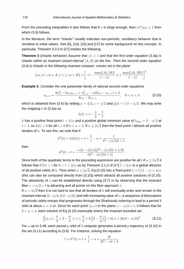
From the preceding inequalities it also follows that if n is large enough, then |c|n|x0| ≤ 1 from
which (3.9) follows.
In the literature, the term “chaotic” usually indicates non-periodic, oscillatory behavior that is
sensitive to initial values. See [5], [14], [15] and [17] for some background on this concept. In
particular, Theorem 3.3.3 in [17] implies the following:
Theorem 3 (chaotic behavior) Assume that |c| < 1 and that the first order equation (3.3a) is
chaotic within an invariant closed interval [A,B] on the line. Then the second order equation
(3.4) is chaotic in the following invariant compact, convex set in the plane
(u, v) : cu + A ≤ v ≤ cu + B ∩[−1 − max|A|, |B|
1 − |c| , 1 +max|A|, |B|
1 − |c|]2
.
Example 3. Consider the one parameter family of rational second order equations
xn+1 =6x2
n − 5xnxn−1 + x2n−1 − α(2xn − xn−1) + 4
4xn − 2xn−1, 0 < α < 4 (3.10)
which is obtained from (3.4) by setting a = 3/2, c = 1/2 and g(t) = 1/t − α/2. We may write
the mapping h in (3.3a) as
h(t) = t − α
2+
1t.
h has a positive fixed point t = 2/α and a positive global minimum value of hmin = 2 − α/2 at
t = 1, so h(t) > 0 for all t > 0 if 0 < α < 4. If α ≤ 2√
2 then the fixed point t attracts all positive
iterates of h. To see this, we note that if
h2(t) = h(h(t)) = t +1t− α +
t
t2 − (α/2)t + 1
then
h2(t) − t =−α[t − (2/α)][t2 − (α/2)t + 1/2]
t[t2 − (α/2)t + 1]
Since both of the quadratic terms in the preceding expression are positive for all t if α ≤ 2√
2 it
follows that h2(t) > t for 0 < t < 2/α so by Theorem 2.1.2 of [17] t = 2/α is a global attractor
of all positive orbits of h. Thus when α ≤ 2√
2, Eq.(3.10) has a fixed point x = t/(1 − c) = 4/α
(this can also be computed directly from (3.10)) which attracts all positive solutions of (3.10).
The attractivity of x can be established directly using (3.7) or by observing that the invariant
fiber v = u/2 + t is attracting and all points on this fiber approach x.
If α > 2√
2 then it is not hard to see that all iterates of h will eventually enter and remain in the
invariant interval [2−α/2, h(2−α/2)] and with increasing value of α, a sequence of bifurcations
of periodic orbits ensues that progresses through the Sharkovski ordering to lead to a period 3
orbit at about α = 3.48. Since for each point (u, v) in the plane, v − u/2 = t, it follows that for
2 < α < 4, each solution of Eq.(3.10) eventually enters the invariant bounded set(u, v) :
u
2+ 2 − α
2≤ v ≤ u
2+ h
(2 − α
2
)∩ (0, 1 + 2h(2 − α/2)]2 (3.11)
For α up to 3.48, each period-p orbit of h uniquely generates a period-p trajectory of (3.10) in
the set (3.11) according to (3.8). For instance, solving the equation
t = h2(t) = t +1t− α +
2t
2t2 − αt + 2
118 International Journal of Applied Mathematics & Statistics

for α > 2√
2 yields the period-2 orbit
τ0 =α −√
α2 − 84
, τ1 =α +
√α2 − 84
.
Now using (3.8) we obtain a period-2 solution of (3.10) as
ξ0 =cτ0 + τ1
1 − c2=
3α +√
α2 − 86
,
ξ1 =cτ1 + τ0
1 − c2=
3α −√α2 − 8
6.
On the other hand, if α is close enough to 4, e.g. α > 3.48, then the trajectories of (3.10) will
exhibit sensitivity to initial conditions and undergo nonperiodic oscillations within the set (3.11).
Remark. As the preceding results show, when |c| < 1 then Eq.(3.4) rather faithfully duplicates
the qualitative behavior of solutions of Eq.(3.3a). When |c| > 1 then it is evident from (3.7) that
solutions of (3.4) are typically unbounded and thus any bounded solutions (including periodic
ones) of (3.4) that correspond to bounded behavior in (3.3a) must be unstable. Therefore,
different qualitative behaviors will be exhibited by (3.4) and (3.3a) when |c| > 1.
The relationship between the solutions of (3.4) and (3.3a) in cases c = ±1 is also different
from |c| = 1. It is worth noting that if φ is linear in its first coordinate, then (1.2) becomes a
special case of Eq.(3.4) with c = 1 (upon re-scaling the mapping φ). With c = 1 (3.7) changes
into a sum (or discrete integral) so the nature of solutions of (3.4) will be qualitatively different
from that of the solutions of (3.3a). In particular, a periodic solution of (3.3a) with a cycle
τ0, . . . , τp−1 can translate into periodic solutions of (3.4) if and only if∑p−1
i=0 τi = 0. Thus there
is a significant loss of periodicity in the second order equation. For more details on the case
c = 1 in certain special cases of Eq.(3.4) see [16], [17] and [19].
3.2 Semiconjugacy by ratios
In this section we assume only that (SC3) holds, i.e., f is homogeneous of degree 1. We do
not put any further restrictions such as (3.2) on the coefficients a, b, c in Eq.(1.4). The solutions
of (1.4) under (SC3) exhibit a very different type of behavior than was the case with (SC1) and
(SC2). In order to avoid singularities in (3.6), solutions of (1.4) that contain zero may be singled
out and treated differently.
Since for each given solution rn of (3.6a) the corresponding solution of (1.4) is obtained from
(3.6b) as
xn = rnrn−1 · · · r0x−1 (3.12)
the following result is easy to establish.
Theorem 4. Let x0, x−1 be given initial values with x−1 = 0 and let rn be a solution of
Eq.(3.6a) with r0 = x0/x−1. Assume that rn is a real number for all n ≥ 0 (e.g. rn is contained
in an invariant set of (3.6a) which does not contain 0). Then the following is true:
(a) If there is n0 ≥ 0 such that |rn| < 1 for all n ≥ n0 then the corresponding solution xn of
(1.4) converges to 0.
Int. J. Appl. Math. Stat.; Vol. 9, No. J07, June 2007 119
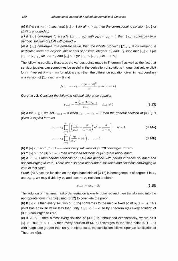
(b) If there is n0 ≥ 0 such that |rn| > 1 for all n ≥ n0 then the corresponding solution xn of
(1.4) is unbounded.
(c) If rn converges to a cycle ρ1, . . . , ρp with ρ1ρ2 · · · ρp = 1 then xn converges to a
periodic solution of (1.4) with period p.
(d) If xn converges to a nonzero value, then the infinite product∏∞
n=0 rn is convergent; in
particular, there are disjoint, infinite sets of positive integers K0 and K1 such that |rn| < 1 (or
|xn| < |xn−1|) for n ∈ K0 and |rn| > 1 (or |xn| > |xn−1|) for n ∈ K1.
The following corollary illustrates the various points made in Theorem 4 as well as the fact that
semiconjugates can sometimes be useful in the derivation of solutions in quantitatively explicit
form. If we set β = a − αc for arbitrary a, c then the difference equation given in next corollary
is a version of (1.4) with b = 0 and
f(v, u − cv) =α(u − cv)2
v+ αc(u − cv).
Corollary 2. Consider the following rational difference equation
xn+1 =αx2
n + βxnxn−1
xn−1, x−1 = 0 (3.13)
(a) If for n ≥ 0 we set xn+1 = 0 when xn−1 = xn = 0 then the general solution of (3.13) is
given in explicit form as
xn = x0
n∏k=1
[(x0
x−1− β
1 − α
)αk +
β
1 − α
], α = 1 (3.14a)
xn = x0
n∏k=1
(x0
x−1+ βk
), α = 1. (3.14b)
(b) If |α| < 1 and |β| < 1 − α then every solutions of (3.13) converges to zero.
(c) If |α| > 1 or |β| > 1 − α then almost all solutions of (3.13) are unbounded.
(d) If |α| = 1 then certain solutions of (3.13) are periodic with period 2, hence bounded and
not converging to zero. There are also both unbounded solutions and solutions converging to
zero in this case.
Proof. (a) Since the function on the right hand side of (3.13) is homogeneous of degree 1 in xn
and xn−1, we may divide by xn and use the rn notation to obtain
rn+1 = αrn + β. (3.15)
The solution of this linear first order equation is easily obtained and then transformed into the
appropriate form in (3.14) using (3.12) to complete the proof.
(b) If |α| < 1 then every solution of (3.15) converges to the unique fixed point β/(1 − α). This
point has absolute value less than unity if |β| < 1 − α so by Theorem 4(a) every solution of
(3.13) converges to zero.
(c) If |α| > 1 then almost every solution of (3.15) is unbounded exponentially, where as if
|α| < 1 but |β| > 1 − α then every solution of (3.15) converges to the fixed point β/(1 − α)with magnitude greater than unity. In either case, the conclusion follows upon an application of
Theorem 4(b).
120 International Journal of Applied Mathematics & Statistics

(d) In this case it is more efficient to use Eq.(3.14). If α = 1 and β = 0 then using (3.14b) it
is clear that every solution of (3.13) is unbounded whereas if β = 0 then solutions with initial
values satisfying |x0| ≤ |x−1| are bounded (periodic if x0 = −x−1 = 0).
If α = −1 then consider solutions with initial values satisfying x0/x−1 = 1 + β/2. For these
solutions (3.14a) reduces to
xn = x0
n∏k=1
[(−1)k +
β
2
]= Kn
(β2
4− 1)[n/2]
where [n/2] is the greatest integer less than or equal to n/2 and Kn = x0 if n is even and
Kn = x0(β/2 − 1) if n is odd. It follows that if |β| ≤ 2√
2 then xn is bounded whereas if
β > 2√
2 then xn is unbounded. In particular, if β = 0,±2√
2 then xn is periodic with
period 2.
To give further applications of ratios, the next two results are quoted from the literature ([9],
[10], [18]) concerning the following equation
xn+1 = |αxn − βxn−1| (3.16)
which is a special case of Eq.(1.4) where a = b = 0 and f(v, u − cv) = α|u − cv| if we define
c = β/α. In this case, Eq.(3.6a) takes the form
rn+1 =∣∣∣∣α − β
rn
∣∣∣∣ (3.17)
Theorem 5. [18] Let α = β = 1 in (3.16) and let Q+ denote the set of all non-negative rational
numbers.
(a) If x0/x−1 ∈ Q+ or x−1 = 0 then the corresponding solution xn of (3.16) has period 3
eventually and for all large n its cycles are 0, α, α where α > 0.
(b) If x0/x−1 /∈ Q+ then the corresponding solution xn of (3.16) converges to zero.
(c) Equation (3.17) has a period-p solution or a p-cycle ρ1, . . . , ρp for every p = 3. These
p-cycles are given as
ρ1 =1 +
√5
2, ρ2 =
√5 − 1√5 + 1
(p = 2)
ρ1 =12
[yp−4 +
√y2
p−4 + 4yp−4yp−1
], ρk =
yk−4ρ1 − yk−2
yk−3 − yk−5ρ1, 2 ≤ k ≤ p, (p ≥ 4)
where yn is the n-th Fibonacci number; i.e., yn+1 = yn + yn−1 for n ≥ −2 where we define
y−3 = −1, y−2 = 1.
(d) If ρ1, . . . , ρp is a periodic solution of (3.17) then for the corresponding solution xn of
(3.16) it is true that
xn = x0ρn/p, if n/p is an integer
xn ≤ x0αρn/p, otherwise
Int. J. Appl. Math. Stat.; Vol. 9, No. J07, June 2007 121

where
ρ =p∏
i=1
ρi < 1, α = maxr1, . . . , rpρ−(1−1/p) > 1.
Theorem 6. [9] (a) Eq.(3.16) has a positive period-2 solution if and only if
β2 − α2 = 1, α > 0.
Further, these period-2 solutions are confined to the pair of lines y = r1x and y = r2x in phase
space, where the slopes r1, r2 are given by
r1 =β − 1
α, r2 =
β + 1α
.
On the other hand, the only period-2 solutions of (3.16) that pass through the origin occur at
α = 0 where β = 1.
(b) Eq.(3.16) has a positive period-3 solution if and only if
α3 + αβ − β3 = 1, α > 1. (3.18)
Further, these period-3 solutions are confined to the three lines y = rix in phase space where
for i = 1, 2, 3, the slopes ri are given by
r1 =αβ + 1α2 + β
, r2 =β2 − α
αβ + 1, r3 =
β + α2
β2 − α. (3.19)
On the other hand, the only period-3 solutions of (3.16) that pass through the origin occur at
α = 1 where β = 1 also (see Theorem... above).
(c) Let β = 1. Then there is a strictly increasing sequence of parameter values αp, p ≥ 3,
such that
α3 = 1 and limp→∞αp = 2
and for each p = 3, 4, 5, . . . the particular solution xn of (3.16) with initial values x−1 = 1,
x0 = αp is periodic with period p.
It is a curious fact that the behaviors of solutions of (3.13) are considerably simpler than those
of (3.16). This is not easy to understand through a direct comparison of the two second order
difference equations which seem to have little in common except that they are both 2-parameter
difference equations. However, the essential difference becomes apparent when we contrast
the relatively simple dynamics of the linear mapping (3.15) with the much more complex dy-
namics of the first order mapping (3.17).
References
[1] Agarwal, R.P., 2000, Difference Equations and Inequalities, 2nd ed., Dekker, New York.
[2] Alseda, L. and Llibre, J. 1993, Periods for triangular maps, Bull. Australian Math. Soc., 47:
41-53.
122 International Journal of Applied Mathematics & Statistics

[3] Berezansky, L., Braverman, E. and Liz, E., 2005, Sufficient conditions for the global stability
of nonautonomous higher order difference equation, J. Difference Eq. and Appl., 11: 785-798.
[4] Burden, R.L. and Fairs, J.D., 1997, Numerical Analysis, 6th ed., Brooks/Cole, Pacific Grove.
[5] Collet, P. and Eckmann, J-P., 1980, Iterated Maps on the Interval as Dynamical Systems,
Birkhauser, Boston.
[6] Elaydi, S.N., 1999, An Introduction to Difference Equations, 2nd ed, Springer, New York.
[7] Greenspan, D., 1973, Discrete Models, #3 in the Applied Math. and Computation Series,
Addison-Wesley, Reading.
[8] Kelley, W. and Petersen, A.C., 2001, Difference Equations: An Introduction with Applica-
tions, 2nd. ed., Academic Press, San Diego.
[9] Kent, C.M. and Sedaghat, H., 2004, Convergence, periodicity and bifurcations for the two-
parameter, absolute difference equation, J. Difference Eq. and Appl., 10: 817-841.
[10] Kent, C.M. and Sedaghat, H., 2005, Difference equations with absolute values, J. Differ-
ence Eq. and Appl., 11: 677-685.
[11] Kloeden, P.E., 1979, On Sharkovsky’s cycle coexistence ordering, Bull. Australian Math.
Soc., 20: 171-177.
[12] Kocic, V.L. and Ladas, G., 1993, Global Behavior of Nonlinear Difference Equations of
Higher Order with Applications, Kluwer, Dordrecht.
[13] Kulenovic, M.R.S. and Ladas, G., 2001, Dynamics of Second Order Rational Difference
Equations with Open Problems and Conjectures, Chapman and Hall/CRC Boca Raton.
[14] Li, T-Y. and Yorke, J.A., 1975, Period 3 implies chaos, Amer. Math. Monthly, 82: 985-992.
[15] Marotto, F.R., 1978, Snap-back repellers imply chaos in Rn, J. Math. Anal. and Appl., 63:
199-223.
[16] Puu, T., 1993, Nonlinear Economic Dynamics, 3rd. ed., Springer, New York.
[17] Sedaghat, H., 2003, Nonlinear Difference Equations: Theory with Applications to Social
Science Models, Kluwer, Dordrecht.
[18] Sedaghat, H., 2004, Periodicity and convergence for xn+1 = |xn − xn−1|, J. Math. Anal.
and Appl., 291: 31-39.
[19] Sedaghat, H., 2005, Global attractivity, oscillations and chaos in a class of nonlinear sec-
ond order difference equations, CUBO Math. J., 7: 89-110.
[20] Sharkovsky, A.N., 1964, Co-existence of cycles of a continuous mapping of the line into
itself, Ukrain. Math. Zh. 16: 61-71 (Russian).
Int. J. Appl. Math. Stat.; Vol. 9, No. J07, June 2007 123

Extended Oligopoly Models and Their Asymptotical Behavior
F. SZIDAROVSZKY
Systems and Industrial Engineering Department University of Arizona
Tucson, AZ 85721-0020, U.S.A Email: [email protected]
ABSTRACT
We will investigate the different extensions of the Cournot oligopoly model including models with intertemporal demand interaction, including production adjustment cost, pollution treatment cost sharing, and cost interaction. The local asymptotic stability of the steady state is examined in all cases and the stability conditions are compared to the classical Cournot model.
KEY WORDS: Dynamic economic systems, oligopoly, asymptotic stability
AMS Mathematic Subject Classification: 91A40, 93A30
INTRODUCTION
Cournot oligopolies, their different variants, extensions and generalizations play an important
role in the literature of mathematical economics. The early results up to the mid 70s are
summarized in Okuguchi (1976), and their multi-product extensions with application studies
are discussed in Okuguchi and Szidarovszky (1999). In the earliest studies the existence and
uniqueness of the Nash-equilibrium of static oligopolies was the central issue, and later the
attention has been turned to the asymptotical properties of the dynamic extensions. Puu and
Sushko (2002) give a comprehensive summary of the most important more recent findings.
All models discussed in the literature so far, are based on certain simplifying assumptions,
which made the simple, analytic examination possible.
In this paper we will drop some of the simplifying assumptions of earlier models and will focus
on more sophisticated models. In particular, we will consider models with intertemporal
demand interaction, production adjustment costs, pollution treatment cost sharing and also
with cost interaction. The simplified versions of some of the models to be discussed in this
paper have been introduced earlier in Okuguchi and Szidarovszky (1999) as well as in the
International Journal of Applied Mathematics & Statistics,ISSN 0973-1377 (Print), ISSN 0973-7545 (Online)Copyright © 2007 by IJAMAS, CESERIJAMAS: June 2007, Vol. 9, No. J07, 124-133
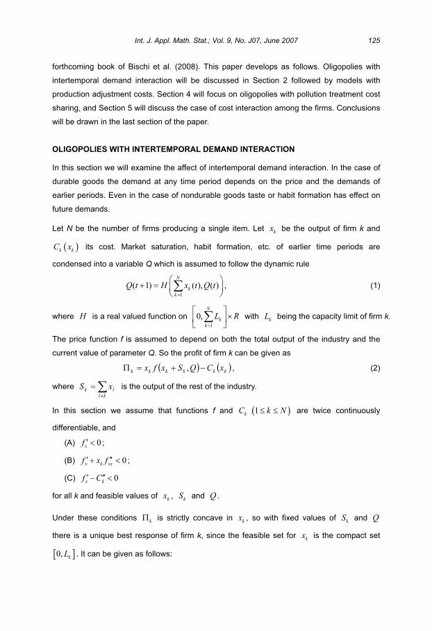
forthcoming book of Bischi et al. (2008). This paper develops as follows. Oligopolies with
intertemporal demand interaction will be discussed in Section 2 followed by models with
production adjustment costs. Section 4 will focus on oligopolies with pollution treatment cost
sharing, and Section 5 will discuss the case of cost interaction among the firms. Conclusions
will be drawn in the last section of the paper.
OLIGOPOLIES WITH INTERTEMPORAL DEMAND INTERACTION
In this section we will examine the affect of intertemporal demand interaction. In the case of
durable goods the demand at any time period depends on the price and the demands of
earlier periods. Even in the case of nondurable goods taste or habit formation has effect on
future demands.
Let N be the number of firms producing a single item. Let kx be the output of firm k and
k kC x its cost. Market saturation, habit formation, etc. of earlier time periods are
condensed into a variable Q which is assumed to follow the dynamic rule
1
( 1) ( ), ( )N
k
k
Q t H x t Q t , (1)
where H is a real valued function on 1
0,N
k
k
L R with kL being the capacity limit of firm k.
The price function f is assumed to depend on both the total output of the industry and the
current value of parameter Q. So the profit of firm k can be given as
kkkkkk xCQSxfx , , (2)
wherekl
lk xS is the output of the rest of the industry.
In this section we assume that functions f and 1kC k N are twice continuously
differentiable, and
(A) 0xf ;
(B) 0x k xxf x f ;
(C) 0x kf C
for all k and feasible values of kx , kS and Q .
Under these conditions k is strictly concave in kx , so with fixed values of kS and Q
there is a unique best response of firm k, since the feasible set for kx is the compact set
0, kL . It can be given as follows:
Int. J. Appl. Math. Stat.; Vol. 9, No. J07, June 2007 125

*
0 if , 0 0
, if , , 0
otherwise,
k k
k k k k x k k k k k k
k
f S Q C
R S Q L L f L S Q f L S Q C L
x
(3)
where *
kx is the unique solution of equation
0,, kkkkxkkk xCQSxfxQSxf (4)
in interval 0, kL . In the first two cases of (3) the partial derivatives of kR are zeros, except
the boundary points. Implicit differentiation shows that in the third case
2
k x k xxk
k x k xx k
R f x fr
S f x f C and
2
Q k xQkk
x k xx k
f x fRr
Q f x f C. (5)
Assumptions (B) and (C) imply that
1 0kr (6)
as it is usual in the theory of discrete concave oligopolies. In addition, assume that
(D) 0Q k xQf x f
for all feasible values of kx , kS and Q . Then
0kr . (7)
Let 0ka denote the speed of adjustment of firm k and assume that the firms change their
outputs in the direction towards their best responses. This dynamism can be mathematically
described by the discrete system
1 , 1k k k k l k
l k
x t x t a R x t Q t x t k N (8)
1
1 ,N
k
k
Q t H x t Q t . (9)
A vector 1, , ,Nx x Q is a steady state of this system if and only if for all k,
,k k l
l k
x R x Q
and
1
,N
k
k
Q H x Q .
The local asymptotical stability of this system can be examined by linearization. The Jacobian
of the system at the steady state can be written as follows:
126 International Journal of Applied Mathematics & Statistics
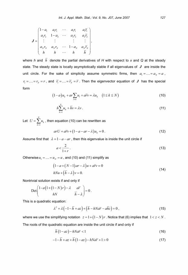
1 1 1 1 1 1 1
2 2 2 2 2 2 2
1
1
1N N N N N N N
a a r a r a r
a r a a r a r
a r a r a a r
h h h h
J ,
where h and h denote the partial derivatives of H with respect to x and Q at the steady
state. The steady state is locally asymptotically stable if all eigenvalues of J are inside the
unit circle. For the sake of simplicity assume symmetric firms, then 1 Na a a ,
1 Nr r r , and 1 Nr r r . Then the eigenvector equation of J has the special
form
1 1k l k
l k
a u ar u arv u k N (10)
1
N
k
k
h u hv v . (11)
Let1
N
k
k
U u , then equation (10) can be rewritten as
1 0karU arv a ar u . (12)
Assume first that 1 a ar , then this eigenvalue is inside the unit circle if
2
1a
r. (13)
Otherwise 1 Nu u u , and (10) and (11) simplify as
1 1 0
0.
a N ar u arv
hNu h v (14)
Nontrivial solution exists if and only if
1- 1 1Det 0
a N r ar
hN h.
This is a quadratic equation:
2 1 0h az h hNar ahz , (15)
where we use the simplifying notation 1 1z N r . Notice that (6) implies that 1 z N .
The roots of the quadratic equation are inside the unit circle if and only if
1 1h az hNar (16)
1 1 1 0h az h az hNar (17)
Int. J. Appl. Math. Stat.; Vol. 9, No. J07, June 2007 127
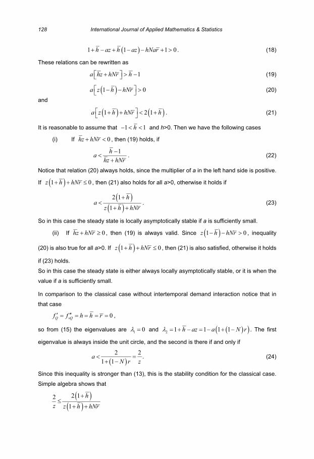
1 1 1 0h az h az hNar . (18)
These relations can be rewritten as
1a hz hNr h (19)
1 0a z h hNr (20)
and
1 2 1a z h hNr h . (21)
It is reasonable to assume that 1 1h and h>0. Then we have the following cases
(i) If 0hz hNr , then (19) holds, if
1ha
hz hNr. (22)
Notice that relation (20) always holds, since the multiplier of a in the left hand side is positive.
If 1 0z h hNr , then (21) also holds for all a>0, otherwise it holds if
2 1
1
ha
z h hNr. (23)
So in this case the steady state is locally asymptotically stable if a is sufficiently small.
(ii) If 0hz hNr , then (19) is always valid. Since 1 0z h hNr , inequality
(20) is also true for all a>0. If 1 0z h hNr , then (21) is also satisfied, otherwise it holds
if (23) holds.
So in this case the steady state is either always locally asymptotically stable, or it is when the
value if a is sufficiently small.
In comparison to the classical case without intertemporal demand interaction notice that in
that case
0Q xQf f h h r ,
so from (15) the eigenvalues are 1 0 and 2 1 1 1 1h az a N r . The first
eigenvalue is always inside the unit circle, and the second is there if and only if
2 2
1 1a
N r z. (24)
Since this inequality is stronger than (13), this is the stability condition for the classical case.
Simple algebra shows that
2 12
1
h
z z h hNr
128 International Journal of Applied Mathematics & Statistics
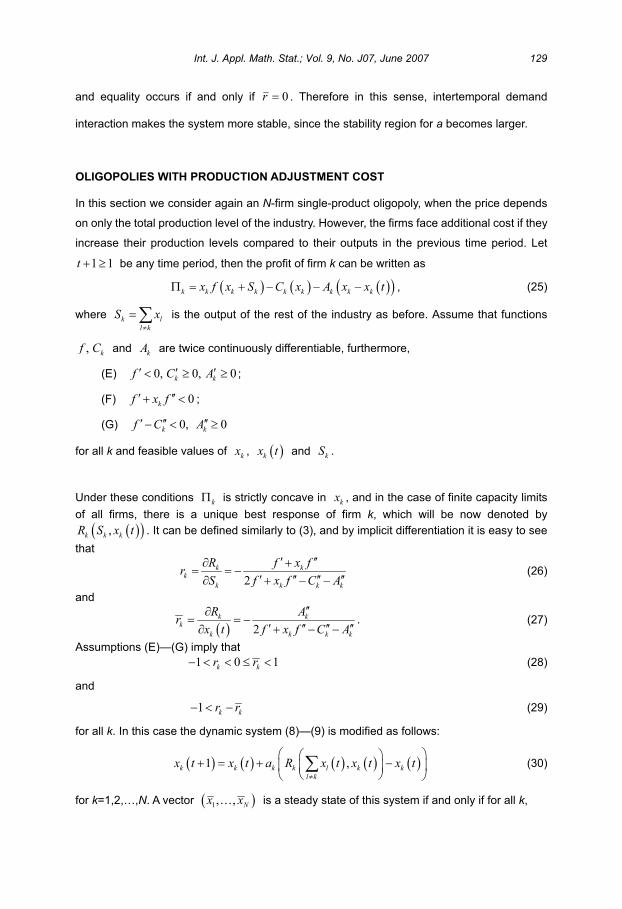
and equality occurs if and only if 0r . Therefore in this sense, intertemporal demand
interaction makes the system more stable, since the stability region for a becomes larger.
OLIGOPOLIES WITH PRODUCTION ADJUSTMENT COST
In this section we consider again an N-firm single-product oligopoly, when the price depends
on only the total production level of the industry. However, the firms face additional cost if they
increase their production levels compared to their outputs in the previous time period. Let
1 1t be any time period, then the profit of firm k can be written as
k k k k k k k k kx f x S C x A x x t , (25)
where k l
l k
S x is the output of the rest of the industry as before. Assume that functions
, kf C and kA are twice continuously differentiable, furthermore,
(E) 0, 0, 0k kf C A ;
(F) 0kf x f ;
(G) 0, 0k kf C A
for all k and feasible values of kx , kx t and kS .
Under these conditions k is strictly concave in kx , and in the case of finite capacity limits
of all firms, there is a unique best response of firm k, which will be now denoted by
,k k kR S x t . It can be defined similarly to (3), and by implicit differentiation it is easy to see
that
2
k kk
k k k k
R f x fr
S f x f C A (26)
and
2
k kk
k k k k
R Ar
x t f x f C A. (27)
Assumptions (E)—(G) imply that 1 0 1k kr r (28)
and
1 k kr r (29)
for all k. In this case the dynamic system (8)—(9) is modified as follows:
1 ,k k k k l k k
l k
x t x t a R x t x t x t (30)
for k=1,2,…,N. A vector 1, , Nx x is a steady state of this system if and only if for all k,
Int. J. Appl. Math. Stat.; Vol. 9, No. J07, June 2007 129
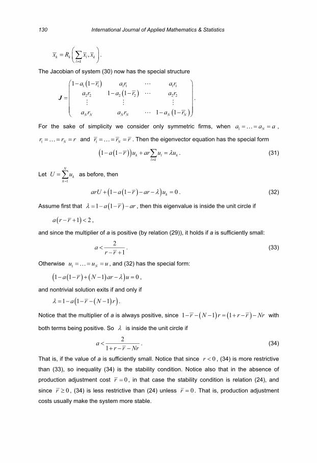
,k k l k
l k
x R x x .
The Jacobian of system (30) now has the special structure
1 1 1 1 1 1
2 2 2 2 2 2
1 1
1 1
1 1N N N N N N
a r a r a r
a r a r a r
a r a r a r
J .
For the sake of simplicity we consider only symmetric firms, when 1 Na a a ,
1 Nr r r and 1 Nr r r . Then the eigenvector equation has the special form
1 1 k l k
l k
a r u ar u u . (31)
Let1
N
k
k
U u as before, then
1 1 0karU a r ar u . (32)
Assume first that 1 1a r ar , then this eigenvalue is inside the unit circle if
1 2a r r ,
and since the multiplier of a is positive (by relation (29)), it holds if a is sufficiently small:
2
1a
r r. (33)
Otherwise 1 Nu u u , and (32) has the special form:
1 1 1 0a r N ar u ,
and nontrivial solution exits if and only if
1 1 1a r N r .
Notice that the multiplier of a is always positive, since 1 1 1r N r r r Nr with
both terms being positive. So is inside the unit circle if
2
1a
r r Nr. (34)
That is, if the value of a is sufficiently small. Notice that since 0r , (34) is more restrictive
than (33), so inequality (34) is the stability condition. Notice also that in the absence of
production adjustment cost 0r , in that case the stability condition is relation (24), and
since 0r , (34) is less restrictive than (24) unless 0r . That is, production adjustment
costs usually make the system more stable.
130 International Journal of Applied Mathematics & Statistics
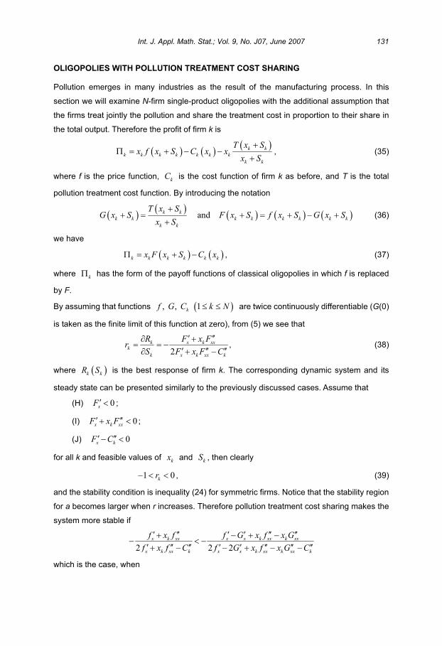
OLIGOPOLIES WITH POLLUTION TREATMENT COST SHARING
Pollution emerges in many industries as the result of the manufacturing process. In this
section we will examine N-firm single-product oligopolies with the additional assumption that
the firms treat jointly the pollution and share the treatment cost in proportion to their share in
the total output. Therefore the profit of firm k is
k k
k k k k k k k
k k
T x Sx f x S C x x
x S, (35)
where f is the price function, kC is the cost function of firm k as before, and T is the total
pollution treatment cost function. By introducing the notation
andk k
k k k k k k k k
k k
T x SG x S F x S f x S G x S
x S (36)
we have
k k k k k kx F x S C x , (37)
where k has the form of the payoff functions of classical oligopolies in which f is replaced
by F.
By assuming that functions , , 1kf G C k N are twice continuously differentiable (G(0)
is taken as the finite limit of this function at zero), from (5) we see that
2
k x k xxk
k x k xx k
R F x Fr
S F x F C, (38)
where k kR S is the best response of firm k. The corresponding dynamic system and its
steady state can be presented similarly to the previously discussed cases. Assume that
(H) 0xF ;
(I) 0x k xxF x F ;
(J) 0x kF C
for all k and feasible values of kx and kS , then clearly
1 0kr , (39)
and the stability condition is inequality (24) for symmetric firms. Notice that the stability region
for a becomes larger when r increases. Therefore pollution treatment cost sharing makes the
system more stable if
2 2 2
x k xx x x k xx k xx
x k xx k x x k xx k xx k
f x f f G x f x G
f x f C f G x f x G C
which is the case, when
Int. J. Appl. Math. Stat.; Vol. 9, No. J07, June 2007 131
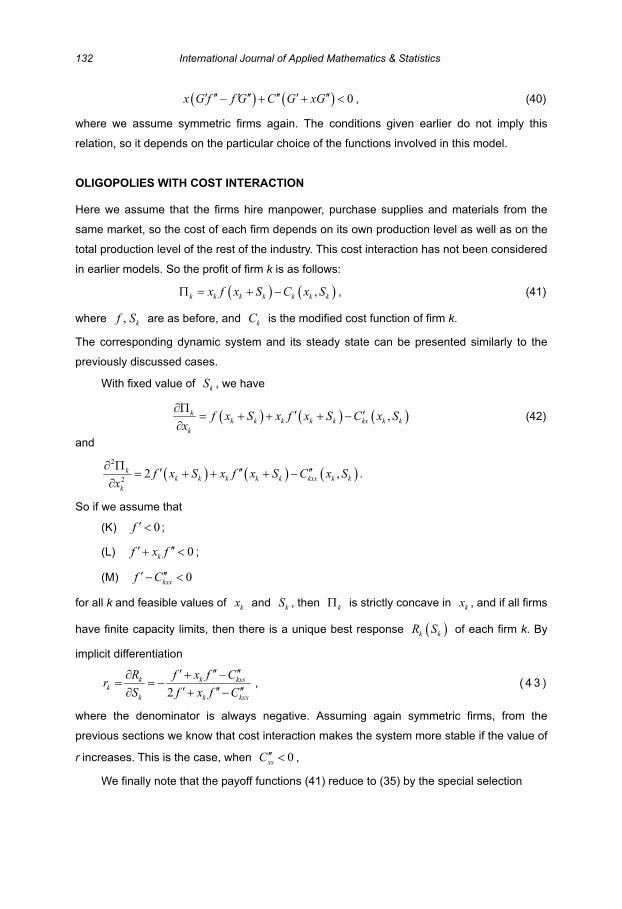
0x G f f G C G xG , (40)
where we assume symmetric firms again. The conditions given earlier do not imply this
relation, so it depends on the particular choice of the functions involved in this model.
OLIGOPOLIES WITH COST INTERACTION
Here we assume that the firms hire manpower, purchase supplies and materials from the
same market, so the cost of each firm depends on its own production level as well as on the
total production level of the rest of the industry. This cost interaction has not been considered
in earlier models. So the profit of firm k is as follows:
,k k k k k k kx f x S C x S , (41)
where , kf S are as before, and kC is the modified cost function of firm k.
The corresponding dynamic system and its steady state can be presented similarly to the
previously discussed cases.
With fixed value of kS , we have
,kk k k k k kx k k
k
f x S x f x S C x Sx
(42)
and
2
22 ,k
k k k k k kxx k k
k
f x S x f x S C x Sx
.
So if we assume that
(K) 0f ;
(L) 0kf x f ;
(M) 0kxxf C
for all k and feasible values of kx and kS , then k is strictly concave in kx , and if all firms
have finite capacity limits, then there is a unique best response k kR S of each firm k. By
implicit differentiation
2
k k kxsk
k k kxx
R f x f Cr
S f x f C, ( 4 3 )
where the denominator is always negative. Assuming again symmetric firms, from the
previous sections we know that cost interaction makes the system more stable if the value of
r increases. This is the case, when 0xsC ,
We finally note that the payoff functions (41) reduce to (35) by the special selection
132 International Journal of Applied Mathematics & Statistics

,k k
k k k k k k
k k
T x SC x S C x x
x S,
so models with pollution treatment cost sharing are special cases of the models of this
section.
CONCLUSIONS
In this paper four extensions of the classical Cournot model were introduced and their local
asymptotical stability was examined.
In the first case we assumed the presence of intertemporal demand interaction in the market
as the result of market saturation, taste or habit formation etc. In the second case we
assumed that any increase in the output level during any time period results in an additional
cost. In the third case the firms treat pollution jointly and share the cleaning cost in proportion
to their share in the total output. In the fourth case we assumed that the cost of each firm
depends on the firm’s own output as well as on the output of the rest of the industry.
For the sake of simplicity we considered only symmetric firms and presented the stability
conditions in term of the common speed of adjustment of the firms. In all cases the condition
requires its value to be sufficiently small. This stability region increases by intertemporal
demand interaction in the market as well as by the presence of production adjustment costs.
Conditions were derived in the other two cases to guarantee the increase of the stability
region. These conditions depend on the particular choice of the cost and price functions.
In the discussions of this paper we assumed symmetric firms for mathematical convenience
only. The general case can be investigated in a similar manner based on the methodology
being discussed in Bischi et al. (2008).
REFERENCES
Bischi, G. I., Chiarella, C., Kopel, M. and Szidarovszky, F., 2008, Nonlinear Oligopolies: Stability and Bifurcations, Amsterdam: Elsevier (forthcoming).
Okuguchi, K., 1976, Expectations and Stability in Oligopoly Models, Berlin/ /New York: Springer-Verlag.
Okuguchi, K. and Szidarovszky, F., 1999, The Theory of Oligopoly with Multi-Product Firms(2nd edition), Berlin/ /New York: Springer-Verlag.
Puu, T. and Sushko, I., (eds.) 2002, Oligopoly Dynamics, Berlin/New York: Springer-Verlag.
Int. J. Appl. Math. Stat.; Vol. 9, No. J07, June 2007 133

Submission of Manuscripts
International Journal of Applied
Mathematics & Statistics (IJAMAS)
ISSN 0973-1377 (Print); ISSN 0973-7545 (Online)
The authors should submit an electronic copy of their unpublished and original paper to the Executive Editor, International Journal of Applied Mathematics & Statistics, Centre for
Environment, Social & Economic Research, Post Box No. 113, Roorkee-247667, INDIA;Email: [email protected]; [email protected]. We strongly encourage electronic submission of manuscript by email to the Executive Editor. It will be assume that authors will keep a copy of their paper. There are no page charges to individuals or institutions for contributions.
Format of Manuscripts:
Instructions for author are available at http://ceser.res.in/ijamas/instr4b.html.
The manuscript should be in the LaTeX or MS Word format. The user of LaTeX should use the journal "LaTeX Style Kit" can be download at http://www.ceser.res.in/ijamas/l-
style.html.
Please send your paper as a single document including tables and figures. This means, it should be one Microsoft Word file ... AND NOT a zipped File containing different files for text, tables, figures, etc. The paper should not normally exceed 5000 words, and should confirm to the following:
The paper should contain the title, author(s) name, affiliation(s), mailing and email
addresses
Abstract describing the context and scope of the paper
Keywords
Mathematics Subject Classification
Main text
References
All pages should be without page number, header Text and footer text.
Submission of a paper implies that the reported work is neither under consideration for a scientific journal nor already published. All manuscripts are subject to peer review. If revisions are required for acceptance of a manuscript, one copy of the revised manuscript should be submitted.
The corresponding author will receive a PDF file of the article via email. This file is for personal use only and may not be copied and disseminated in any form without prior written permission from journal.
Print copy of the journal will be dispatch to subscribers only. A free print (paper) issue of journal will be available to the authors whose institutions subscribe. A copy of single issue of journal is available on a special discount to the authors only. Furthermore, you are welcome to support the journal by requesting that your library to subscribe the journal, or by taking out an individual subscription.

The IJAMAS is reviewed, abstracted and indexed by the Mathematical Reviews
(MathSciNet), Zentralblatt MATH, Statistical Theory and Method Abstracts (STMA-Z),
Current Index to Statistics (CIS) [ The Current Index to Statistics (CIS) is a joint venture of the American Statistical Association & Institute of Mathematical Statistics, USA],International Abstracts in Operations Research (IAOR), Indian Science
Abstracts, JournalSeek and Getcited.
The views and contents of the articles (papers) printed in this issue herein do not reflect the official views of International Journal of Applied Mathematics & Statistics (IJAMAS) and Editors of the journal. The concern author(s) is answerable for the correctness (or plagiarism) and authenticity of article.
SUBSCRIPTIONS
Followings are the Annual Subscription Fee for year 2007 of International Journal of Applied Mathematics & Statistics (IJAMAS):
Issue Individual Institutional
Print Issue: Euro € /US$ 700.00 Euro € /US$ 1000.00
Online: Euro € /US$ 300.00 Euro € /US$ 700.00
Print Issue and Online (Both): Euro € /US$ 800.00 Euro € /US$ 1500.00
How to Pay Subscriptions?
Subscriptions are payable in advance. Subscribers are requested to send payment with their order. Issues will only be sent on receipt of payment. Subscriptions are entered on an annual basis and may be paid US Dollars/Euro or in equivalent amount in Indian Rupees.
Payment can be made by Bank Draft/ Bank Wire Transfers only. All payments should be made to "Centre for Environment, Social & Economic Research" bank draft should be drawn on Roorkee, India.
Claims and Cancellations
Claims for issues not received should be made in writing within three months of the date of publication. Cancellations: no refunds will be made after the first issue of the journal for the year has been dispatched.
Detailed information and instructions are available at
http://www.ceser.res.in/ijamas.html
Call for Paper
International Journal of Ecology & Development
The main aim of the International Journal of Ecology & Development (IJED), ISSN
0973-7308 (Online); ISSN 0972-9984 (Print), is to publish refereed, well-written original research articles, and studies that describe the latest research and developments in ecology and development. It also covers the many potential applications and connections to other areas of Ecological Science, economics and technology such as the use and development of mathematics/statistics in ecology or use and development of economics for ecology & development or inter-disciplinary nature of applications for Ecology & Development. IJED is published one Volume per year, three issues yearly in Winter, Summer and Fall. Detailed