Copyright 2004, Society of Petroleum Engineers Inc. This paper was prepared for presentation at the SPE Annual Technical Conference and Exhibition held in Houston,Texas U.S.A., 26 – 29 September 2004. This paper was selected for presentation by an SPE Program Committee following review of information contained in an abstract submitted by the author(s). Contents of the paper, as presented, have not been reviewed by the Society of Petroleum Engineers and are subject to correction by the author(s). The material, as presented, does not necessarily reflect any position of the Society of Petroleum Engineers, its officers, or members. Papers presented at SPE meetings are subject to publication review by Editorial Committees of the Society of Petroleum Engineers. Electronic reproduction, distribution, or storage of any part of this paper for commercial purposes without the written consent of the Society of Petroleum Engineers is prohibited. Permission to reproduce in print is restricted to an abstract of not more than 300 words; illustrations may not be copied. The abstract must contain conspicuous acknowledgment of where and by whom the paper was presented. Write Librarian, SPE, P.O. Box 833836, Richardson, TX 75083-3836, U.S.A., fax 01-972-952-9435.

Abstract The Barnett Shale of North Texas is an ultra low permeability reservoir that must be effectively fracture stimulated in order to obtain commercial production. As a result, techniques to optimize hydraulic fracturing effectiveness have evolved over the past decade. The first Barnett Shale “discovery” well, the C.W. Slay #1, was drilled in 1981 and it was almost 17 years before any significant commercial success was found in the Barnett, so the Barnett is a relatively new play. In fact, 75% of the producing wells in the Barnett have been drilled since 2000. In 1995, when the USGS was performing a gas in place assessment of the significant gas fields in the United States, the Barnett was not even evaluated. In 2002, according to the Energy Information Administration, the Newark East Field produced 202 Bcf, more than any other field in Texas, and was the 7th largest gas producer in the United States! In some areas of the Barnett, horizontal drilling has recently been applied in an attempt to optimize gas production. Issues such as nearby water bearing intervals, inadequate surface locations, improved gas production rates and cost per scf can, in some cases, be addressed by the use of horizontal wellbores. The goal is to maximize fracture network surface area in the targeted pay intervals, and in some areas, reduce the probability of excessive fracture height growth. Several horizontal completion techniques have recently been utilized, including single and multiple stage treatments with multiple perforation clusters in uncemented casing and multiple stage treatments performed in cemented perforated casing. In order to understand created fracture geometry for various completion designs, fracture treatments are often mapped with microseismic and tilt sensors.

Production results from this pilot study of the first twenty-three horizontal wells in the same general “Core” area of the Fort Worth Basin are compared in addition to mapped fracture geometry from eleven of these with vertical wellbores. This paper will discuss drilling and completion strategies, look at fracture network areas obtained from each, and then compare and contrast the fracture effectiveness with the standard procedures used in vertical Barnett wells.

Introduction The current commercial success of Barnett Shale development programs actually has its roots in the 1998 paradigm shift in stimulation techniques. Prior to that time, most Barnett Shale wells were completed with massive hydraulic fracture treatments using crosslinked gelled fluids carrying a few hundred thousand pounds to more than one million pounds of proppant. Because of the extremely low permeability of the Barnett, its inability to efficiently clean up fracture damage from gels, and the high cost of massive hydraulic stimulations, most Barnett treatments did not provide an adequate investment return. In 1998, Devon Energy experimented with an old fracturing technique that was gaining new acceptance at the time in East Texas. The technique was light sand fracturing or “water fracs”1. In many reservoirs, such as the East Texas Cotton Valley Sand, light sand fracturing is used to reduce stimulation costs without decreasing production. In the Barnett Shale, this technique has been successful and is now widely used for a different reason: it provides a much larger surface area of contact with the reservoir and minimizes fracture face damage resulting in improved productivity. Today, nearly every Barnett treatment is performed using light sand fracturing or some permutation of this technique and it has proven to be the most important advancement in the resurgence of Barnett Shale development programs for operators in this basin.

Even with the success enjoyed with light sand fracturing treatments, not every area of the Barnett has proven as successful to date as the “core” area in Wise and Denton Counties. The Barnett Shale covers a large area, from the Fort Worth Basin out past the Permian Basin of West Texas and New Mexico, and the quality and quantity of Barnett pay varies substantially from the traditional core area to the newer plays on the fringes. Successful development in the newer

SPE 90051

Optimizing Horizontal Completion Techniques in the Barnett Shale Using Microseismic Fracture Mapping M.K. Fisher, SPE, Pinnacle Technologies, J.R. Heinze, C.D. Harris, SPE, Devon Energy Corporation, B.M Davidson, C.A. Wright, and K.P. Dunn, SPE, Pinnacle Technologies

2 SPE 90051

CORE AREA

Figure 1 Extent of Barnett Shale with “Core” Area of Wise/Denton Counties outlined areas will likely require additional changes in completion techniques and several new strategies are being tested in both “core” and “fringe” areas of the Barnett Shale. Barnett Basics. The Mississippian-age Barnett Shale is a marine shelf deposit that unconformably lies on the Ordovician-age Viola Limestone / Ellenburger Group and is conformably overlain by the Pennsylvanian-age Marble Falls Limestone. The Barnett Shale within the Fort Worth Basin ranges from 200 to 800 feet in thickness and is approximately 300 - 500 feet thick in the core area of the field. The productive formation is typically described as black, organic-rich shale composed of fine grained, non-siliciclastic rocks with extremely low permeability, ranging from 0.00007 to 0.0005 millidarcies. The Barnett is believed to be its own source rock and is abnormally pressured in the core area. Hydraulic fracture treatments are necessary for commercial production due to the ultra low matrix permeability. Barnett Shale completions in the core area of the Fort Worth Basin have historically consisted of vertical cased wellbores with light sand “waterfracs” consisting of large slickwater volumes (500,000 to 1,500,000 gal) carrying about 75,000 to 250,000 lbm of sand (proppant concentrations range from 0.1 ppg up to 1.0 ppg) and pumped at 45 to 75 bbl/min. The lack of gel solids is believed to contribute to longer and more complex fracture networks with few of the gel cleanup issues that a more viscous fluid system may impose. In the core areas, most wells are completed and stimulated in this manner. In some of the new “fringe” areas, formation properties may dictate a different approach in well construction, completion, and stimulation. Fracture mapping has been used extensively in the core area to determine infill well spacing and locations, to evaluate various stimulation treatment designs and techniques, to identify re-frac candidates, determine staging effectiveness and to test alternative techniques prior to their introduction in the fringe areas of Barnett exploitation.

Conclusions from an earlier study of vertical Barnett stimulation treatments in the core area are as follows 7:

1. Fractures in the Barnett Shale grow in a complex network.

2. The total fracture network length and area, not conventional fracture half-length, controls gas recovery and drainage patterns.

3. Fracture growth in the Barnett Shale can be approximately modeled.

4. Fractures can be propagated simultaneously in the Upper & Lower Barnett during the same fracture treatment.

5. Fracture geometry is relatively predictable; however, fracture network development is highly variable.

6. Fracture height growth is well contained within the Upper and Lower Barnett Shale.

Several of the areas currently under development outside

the core area contain a Barnett interval that is not as well-bounded above and, more importantly, lacks a significant frac barrier below the Barnett Shale interval. To make matters more challenging, the Viola and/or Ellenberger formations below the Lower Barnett Shale are often 100% water-saturated. If a hydraulic fracture grows downward out of the Lower Barnett interval, it could conceivably open a conductive path directly into a porous, water-producing interval, which could be extremely detrimental to relative permeability and subsequent production.

Figure 2 Type Log of “Core” Barnett Interval Showing Overlying and Underlying Limestones

SPE 90051 3

Fracture Evaluation. Numerous fracture diagnostic technologies have been employed to evaluate Barnett Shale fracture effectiveness: real-time fracture modeling, production and well-test analysis, radioactive tracers, production logging, surface tiltmeter mapping, downhole tiltmapping and microseismic fracture mapping. Most of the recent fracture mapping has been performed with microseismic (extremely high-resolution VSP-type geophone sensors) equipment, which “listen” for the slippage events that accompany a hydraulic fracture and then locates those slippages in 3-D space to create a near real-time map of where the fracture is growing. However, in some instances, suitable offset wells are not available for microseismic mapping and surface tiltmeters are used to determine fracture placement effectiveness and orientation. Surface tiltmeters are very valuable on horizontal completions because they can measure fracture orientation(s) and determine slurry volume distribution along the lateral. This answers the question “Does the majority of the slurry go only in the heel, the middle, or the toe of the lateral, or is it evenly distributed along its length?” A key insight from surface tiltmapping in the Barnett was that the cross-cutting (NW-SE) fractures were indeed opening up and represented a significant portion (20 – 60%) of the total created fracture volume. Many technical publications are available which present more detailed information on these commonly used fracture diagnostic tools 2,3,4,5,6.

On this pilot horizontal well completion project, Barnett

fracture treatments are discussed in eleven horizontal wellbores mapped in the core area of the Fort Worth Basin with microseismic sensors. Of these, six wells were completed with uncemented liners and five with cemented liners. Previous fracture mapping projects had identified that fracture growth in vertical Barnett wells was extremely complex, 7 with major fracture growth in at least two vertical orientations (hydraulic fracture growth NE to SW and natural fractures activated NW to SE). This type of multiplanar fracture growth is relatively uncommon and has only been measured in a handful of reservoirs to date. The large fracture “fairways” on these vertical wells were typically about one mile long and about 500 - 1200 ft in width. Good correlation was seen between fracture fairway width and cumulative production i.e. the wider the fracture fairway, the better the cumulative production. Ten month cumulative production was more than sufficient to predict a Barnett well’s estimated ultimate recovery (EUR).

Figure 3 Examples of increasing fracture complexity from simple (most common) to extremely complex (relatively rare). The Figure 3.C (“Extremely Complex”) example is typical of fracturing in the Barnett; the long axis of the fracture network

or “fairway” (oriented ~N40E in the core area of the Fort Worth Basin) is referred to as the hydraulic fracture “fairway length” while the short axis of the rectangle (from NW to SE) is typically referred to as “fairway width”. For vertical wells, these fairway dimensions can approach about one mile in length and up to 1200 ft in width. Figure 4 shows a typical fracture fairway network from a vertical well in the core area of the Barnett. The microseismic events are shown as points on this plan view and the gross fracture area is immediately obvious. The points can be analyzed with time and a linear regression algorithm applied to identify events that happen sequentially and appear to be related to a specific fracture structure. These sequential linear structures are highlighted with lines representing the minimum number and size of likely fracture segments.

-3000

-2500

-2000

-1500

-1000

-500

0

500

1000

1500

-1500 -1000 -500 0 500 1000 1500 2000 2500 3000

West - East (ft)

Rowan 1

Rowan 2

Rowan 3

Spain 2

Spain 3

Cox 6

Rowan 5

-3000

-2500

-2000

-1500

-1000

-500

0

500

1000

1500

-1500 -1000 -500 0 500 1000 1500 2000 2500 3000

West - East (ft)

Killed 1

Killed 2

Killed 3

Killed 4

Killed 5

Figure 4 Example of fracture treatment map in vertical well from core area of Barnett. This well’s fracture length is more than 4000 ft long (2000 ft half-lengths) and “fairway” width is about 1000 ft across. The individual fracture structures are shown as line segments on the map; total fracture network length on this treatment was about 30,000 ft. The five small squares seen just outside the fracture network show the locations of wells that were temporarily killed by the frac treatment on this well. Most fractures mapped around the world to date fall into the “simple” or “slightly complex” description with fracture growth dominantly occurring in only one planar orientation. It is important to recognize that it is virtually impossible with existing fracture mapping tools to measure the difference between fracture illustrations 3.A and 3.B. If the secondary fractures grow nearby and parallel to one another, they must be inferred from fracture pressure diagnostics. Complex parallel fractures (Fig. 3.B) have been physically observed in several core-through and fracture mine-back experiments8. Fracture mapping with microseismic sensors was performed in an effort to better understand the geometry obtained with horizontal well completions compared to that of typical vertical Barnett wells.

A. Simple Fracture B. Complex Fracturing C. Extremely Complex

4 SPE 90051

Horizontal Drilling. It is recognized that horizontal wells will provide greater wellbore contact with a larger volume of reservoir rock than do vertical wells, thus providing the ability to improve development economics. Horizontal wellbores have also been used in an attempt to spread the hydraulic fracturing energy over a larger area, theoretically decreasing the likelihood of excessive fracture height growth into unfavorable intervals. Additionally, some areas in the Fort Worth Basin present special challenges with surface locations based on optimum well density. Housing additions, surface access and landowner restrictions can prevent drilling vertical wells in sufficient density to adequately drain the low-permeability Barnett Shale. Consequently, pad drilling of horizontal wells from a minimum number of surface locations is a viable option to reduce the footprint caused by multiple wellbores and still retain the ability to contact large areas of this productive resource. It is important to note that for all horizontal completions discussed in this paper, the wellbore orientation was roughly NW to SE (in the direction of the least principal stress) so that the fracture fairways would be created transverse to the horizontal lateral’s orientation. The initial stimulation treatment sizes were designed to cover the same fracture pattern that would have been achieved with the drilling of multiple vertical wells over the same area. If the horizontal well traversed an area that would have been drained by three vertical wells, the fracture stimulation volume for the horizontal well was typically three times the volume of a vertical treatment. Lateral lengths in this core area are largely determined by how many undrilled locations can be accessed with the horizontal wellbore. Since vertical well density is high, some horizontal wellbores may be only 2000 ft in length, designed to replace two vertical wells while some are 3000 ft or longer, designed to replace 3 or more vertical wellbores.

Figure 5 Expected Fracture Fairways for Vertical and Horizontal Wellbores

Figure 5 illustrates the fracture geometries that might result from a vertical wellbore (a), a horizontal wellbore drilled in the direction of maximum stress (b), and 3 frac stages in a horizontal well drilled in the direction of the least principal stress (c). Most hard rock formations that are drilled horizontally are drilled similar to (c), generating transverse

fractures cutting across the wellbore, each simulating a single vertical well. In higher permeability environments, (b) might be preferable because it is easier to place wider, more conductive fractures in this configuration. This horizontal pilot was performed in the core area where well control and production of vertical wells are well known. The production of these horizontal wells can thus be directly compared with vertical wells to determine optimum completion strategy prior to implementing horizontal completions in the fringe areas. Hydraulic fracturing in horizontal wells raises the following questions: 1. Cemented vs. Uncemented liners, which is optimal? 2. Single Stage vs. Multiple Stages. Can a single limited

entry treatment cover the entire length of a long horizontal lateral?

3. Will multiple stages divert and provide effective coverage along an uncemented lateral? In a cemented lateral?

4. Do both the Upper and Lower Barnett fracture even though the wellbore is placed only in the Lower Barnett? Will the fractures stay contained within the Barnett interval?

5. What direction should the lateral be oriented based on previous experience with preferred hydraulic and natural fracture orientations?

6. How long should the lateral extend? Many of these issues can be evaluated through the integration of fracture mapping tools such as microseismic mapping with fracture engineering and production correlations. Uncemented Horizontal Wells. All Barnett horizontal wells to date have been cased for borehole stability over the expected long well life and for ease of future well intervention procedures. These cased laterals have been, in numbers, almost equally cemented or uncemented. The horizontal section can be 1000 - 4000 ft in length or more. The ability to effectively stimulate long uncemented laterals is the biggest challenge in performing a fracture treatment on this type of well. Stimulation techniques such as limited entry diversion treatments (determining optimum perforation size, spacing and number and pumping the treatment at a sufficiently high rate to ensure that all perforations must accept fracturing slurry) are used in an attempt to initiate fractures in multiple locations along the wellbore. If this is not successful, the treatment might simply seek its own preferred location(s) along the lateral and leave much of the interval unstimulated. A typical single-stage uncemented horizontal fracture treatment ranges from 1,825,000 to 4,200,000 gallons transporting 500,000 to 1,000,000 lbm of 20/40 and 40/70 Ottawa sand. With fracture volumes this large, even “light sand” treatments can employ a million pounds or more of proppant! The completion process is predicated on casing diameter and strength. Pumping rates approaching 140 bbl/min are achievable with 5-1/2 in, 17 lbm/ft, N-80 casing and up to 200 bbl/min in 7 in, 29 lbm/ft, P-110 casing. The

SPE 90051 5

limited entry perforating design of hole size and number of holes is engineered based on the available treatment rate and designed to maintain a 500 psi differential for each interval. Previous microseismic mapping studies7 on vertical wells indicated minimum fracture fairway widths of 500 ft. Therefore, perforation clusters are typically separated by 500 ft between intervals to obtain complete coverage with the fracture treatments. This design for 5-1/2 in casing typically equates to 50 or 60, 0.45 inch diameter holes spaced in four to five clusters along the horizontal section. When the horizontal section becomes longer, multiple stages are required for effective coverage. A typical single-stage uncemented horizontal completion is a lower cost treatment than multiple stages and typical cumulative stimulation volumes may also be lower than with multiple staging. Multiple stages are designed identical to the single stage treatments with the wellbore generally separated into equal sections. The same limited entry design is applied with the 500 ft perforation spacing and number of holes. Composite frac plugs are set following the first stage treatment to isolate the previously stimulated section of the wellbore. The previously stimulated sections of the reservoir are somewhat isolated from the subsequent stages by a stress diversion effect. The stress diversion effect is present when the reservoir has been “supercharged” by the previous fracture treatment. Stress in this region is increased due to locally higher fluid pressure and to increased stress from propped fractures created by the stimulation treatment. These two isolation means (one mechanical and one due to increased stress) influence the subsequent stage(s) to stimulate reservoir areas that were not treated in the previous stage(s).

Figure 6 Plan View Fracture Map of Typical Uncemented Barnett Treatment with Fracture Structures Illustrated Figure 6 shows an example of a typical uncemented horizontal Barnett stimulation treatment. Treatment volume was 4,200,000 gals slickwater and 853,000 lbm Ottawa sand. The

single-stage fracture treatment was pumped at 130 bbl/min through five sets of perforations. As can be seen, the fracture fairway half-length at each fairway location is about 1000 ft, shorter than a typical vertical well’s fairway. The four fairways’ “widths” average about 500 ft each, narrower than an average fairway on a typical vertical well, but the cumulative fairway width (summing the four fairway’s individual widths) is about 2000 ft, nearly the same as the length of the 2400 ft lateral, as would be expected if the entire lateral is completely stimulated. Note how the fractures do not always initiate adjacent to the perforations. Instead, fracture fluid may travel along the wellbore until a weakness in the rock is encountered, at which point the fracture grows transversely away from the wellbore. This can lead to “gaps” in the fracture network where less than the entire length of the lateral is stimulated. These gaps in the fracture network equate to smaller overall fracture surface area, and can result in lower well productivity.

Figure 7 shows a side view of another Barnett fracture treatment. This is a two-stage fracture treatment in an uncemented wellbore where two conclusions are evident; the second stage treatment diverted sufficiently toward the heel and away from the first stage to effectively cover the entire length of the lateral, and the fracture height was confined to the Lower Barnett only. There is no measurable growth downward into the Viola and no upward growth into the Upper Barnett. Of the 11 wells mapped, both cemented and uncemented, 6 wells exhibited fracture growth only in the Lower Barnett while 5 wells had measurable fracture height growth into the Upper Barnett as well. This upward height growth may be more dependant on the thickness and integrity of the Forestburg Limestone interval than on whether the lateral was cemented or uncemented. None of the wells in this core area study had appreciable growth downward into the Viola/Ellenberger section.

Figure 7 Side View Fracture Map looking normal to uncemented lateral of Barnett treatment with Fracture Height confined to Lower Barnett only. Events shown are for 2 fracture stages. Stage 1 treatment, (filled diamonds) appears to have grown slightly higher than Stage 2 (open diamonds).

5800

6000

6200

6400

6600

6800

7000

7200

7400

7600

7800

8000

8200

8400

8600

8800

9000

-300

0

-280

0

-260

0

-240

0

-220

0

-200

0

-180

0

-160

0

-140

0

-120

0

-100

0

-800

-600

-400

-200 0

200

Distance Along Wellbore (ft)

Dep

th (f

t)

Upper Barnett

Lower Barnett

NW SE

Stage 1Stage 2

5800

6000

6200

6400

6600

6800

7000

7200

7400

7600

7800

8000

8200

8400

8600

8800

9000

-300

0

-280

0

-260

0

-240

0

-220

0

-200

0

-180

0

-160

0

-140

0

-120

0

-100

0

-800

-600

-400

-200 0

200

Distance Along Wellbore (ft)

Dep

th (f

t)

Upper Barnett

Lower Barnett

NW SE5800

6000

6200

6400

6600

6800

7000

7200

7400

7600

7800

8000

8200

8400

8600

8800

9000

-300

0

-280

0

-260

0

-240

0

-220

0

-200

0

-180

0

-160

0

-140

0

-120

0

-100

0

-800

-600

-400

-200 0

200

Distance Along Wellbore (ft)

Dep

th (f

t)

Upper Barnett

Lower Barnett

NW SE

Stage 1Stage 2

-4000.00

-3600.00

-3200.00

-2800.00

-2400.00

-2000.00

-1600.00

-1200.00

-800.00

-400.00

0.00

400.00

800.00

1200.00

1600.00

2000.00

-280

0

-240

0

-200

0

-160

0

-120

0

-800

-400 0

400

800

1200

1600

2000

2400

2800

West-East (ft)

Sout

h-N

orth

(ft)

Fairway “Width”

Fairway “Length”

-4000.00

-3600.00

-3200.00

-2800.00

-2400.00

-2000.00

-1600.00

-1200.00

-800.00

-400.00

0.00

400.00

800.00

1200.00

1600.00

2000.00

-280

0

-240

0

-200

0

-160

0

-120

0

-800

-400 0

400

800

1200

1600

2000

2400

2800

West-East (ft)

Sout

h-N

orth

(ft)

Fairway “Width”

Fairway “Length”

6 SPE 90051

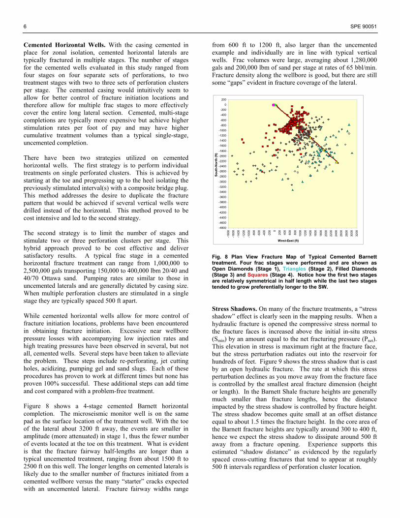
Cemented Horizontal Wells. With the casing cemented in place for zonal isolation, cemented horizontal laterals are typically fractured in multiple stages. The number of stages for the cemented wells evaluated in this study ranged from four stages on four separate sets of perforations, to two treatment stages with two to three sets of perforation clusters per stage. The cemented casing would intuitively seem to allow for better control of fracture initiation locations and therefore allow for multiple frac stages to more effectively cover the entire long lateral section. Cemented, multi-stage completions are typically more expensive but achieve higher stimulation rates per foot of pay and may have higher cumulative treatment volumes than a typical single-stage, uncemented completion. There have been two strategies utilized on cemented horizontal wells. The first strategy is to perform individual treatments on single perforated clusters. This is achieved by starting at the toe and progressing up to the heel isolating the previously stimulated interval(s) with a composite bridge plug. This method addresses the desire to duplicate the fracture pattern that would be achieved if several vertical wells were drilled instead of the horizontal. This method proved to be cost intensive and led to the second strategy. The second strategy is to limit the number of stages and stimulate two or three perforation clusters per stage. This hybrid approach proved to be cost effective and deliver satisfactory results. A typical frac stage in a cemented horizontal fracture treatment can range from 1,000,000 to 2,500,000 gals transporting 150,000 to 400,000 lbm 20/40 and 40/70 Ottawa sand. Pumping rates are similar to those in uncemented laterals and are generally dictated by casing size. When multiple perforation clusters are stimulated in a single stage they are typically spaced 500 ft apart. While cemented horizontal wells allow for more control of fracture initiation locations, problems have been encountered in obtaining fracture initiation. Excessive near wellbore pressure losses with accompanying low injection rates and high treating pressures have been observed in several, but not all, cemented wells. Several steps have been taken to alleviate the problem. These steps include re-perforating, jet cutting holes, acidizing, pumping gel and sand slugs. Each of these procedures has proven to work at different times but none has proven 100% successful. These additional steps can add time and cost compared with a problem-free treatment. Figure 8 shows a 4-stage cemented Barnett horizontal completion. The microseismic monitor well is on the same pad as the surface location of the treatment well. With the toe of the lateral about 3200 ft away, the events are smaller in amplitude (more attenuated) in stage 1, thus the fewer number of events located at the toe on this treatment. What is evident is that the fracture fairway half-lengths are longer than a typical uncemented treatment, ranging from about 1500 ft to 2500 ft on this well. The longer lengths on cemented laterals is likely due to the smaller number of fractures initiated from a cemented wellbore versus the many “starter” cracks expected with an uncemented lateral. Fracture fairway widths range

from 600 ft to 1200 ft, also larger than the uncemented example and individually are in line with typical vertical wells. Frac volumes were large, averaging about 1,280,000 gals and 200,000 lbm of sand per stage at rates of 65 bbl/min. Fracture density along the wellbore is good, but there are still some “gaps” evident in fracture coverage of the lateral.

Fig. 8 Plan View Fracture Map of Typical Cemented Barnett treatment. Four frac stages were performed and are shown as Open Diamonds (Stage 1), Triangles (Stage 2), Filled Diamonds (Stage 3) and Squares (Stage 4). Notice how the first two stages are relatively symmetrical in half length while the last two stages tended to grow preferentially longer to the SW.

Stress Shadows. On many of the fracture treatments, a “stress shadow” effect is clearly seen in the mapping results. When a hydraulic fracture is opened the compressive stress normal to the fracture faces is increased above the initial in-situ stress (Smin) by an amount equal to the net fracturing pressure (Pnet). This elevation in stress is maximum right at the fracture face, but the stress perturbation radiates out into the reservoir for hundreds of feet. Figure 9 shows the stress shadow that is cast by an open hydraulic fracture. The rate at which this stress perturbation declines as you move away from the fracture face is controlled by the smallest areal fracture dimension (height or length). In the Barnett Shale fracture heights are generally much smaller than fracture lengths, hence the distance impacted by the stress shadow is controlled by fracture height. The stress shadow becomes quite small at an offset distance equal to about 1.5 times the fracture height. In the core area of the Barnett fracture heights are typically around 300 to 400 ft, hence we expect the stress shadow to dissipate around 500 ft away from a fracture opening. Experience supports this estimated “shadow distance” as evidenced by the regularly spaced cross-cutting fractures that tend to appear at roughly 500 ft intervals regardless of perforation cluster location.

-4800

-4600

-4400

-4200

-4000

-3800

-3600

-3400

-3200

-3000

-2800

-2600

-2400

-2200

-2000

-1800

-1600

-1400

-1200

-1000

-800

-600

-400

-200

0

200

-180

0

-160

0

-140

0

-120

0

-100

0

-800

-600

-400

-200 0

200

400

600

800

1000

1200

1400

1600

1800

2000

2200

2400

2600

2800

3000

3200

West-East (ft)

Sout

h-N

orth

(ft)

SPE 90051 7

Figure 9 Graph showing relationship between Closure Stress increase and distance away from fracture (Stress Shadow) as a function of fracture height. From Warpinski et al9. Stress shadow effects have been discussed for over 15 years and documented with fracture mapping data for ten years9,10,11,12,13. But they were confined to special cases of tightly-spaced wellbores, and were mostly due to long-term production / injection operations. The advent of horizontal well fracturing changed everything. Now stress shadow effects are critical to the daily design of horizontal well completions and fracture treatment strategy. However the importance of stress shadows remains underappreciated. Stress shadows in horizontal well fracturing have two major impacts: · increased compressive stress near a fracture tends to “close-off” or inhibit the initiation of nearby parallel fractures, providing a natural diversion mechanism along the wellbore. If perf clusters / fracture initiation points are too close together, stress shadows tend to inhibit fracture growth along the mid-section of horizontal wellbores and encourage fracture growth at the heel and toe of wellbores. · increase in the local minimum stress magnitude tends to encourage fracture growth in orthogonal directions. Even in fields where fracture orientation in vertical wells is relatively uniform, stress shadow effects often induce orthogonal fracture growth when stimulating long intervals in horizontal wells. These impacts are illustrated in Figure 10. Both effects are important in the Barnett Shale horizontal well completions. The growth of orthogonal vertical fractures - so-called “fracture networks” - occurs even in vertical wells in the Barnett Shale due to a low in-situ horizontal deviatoric stress and the presence of natural fractures orthogonal to today’s maximum stress direction (NE-SW). Stress shadows from simultaneously growing and competing fractures initiated along a horizontal wellbore tend to further enhance fracture growth in the orthogonal direction (NW-SE). This is a good thing as reservoir contact area (network size) and network density are both thought to contribute to well productivity.

Figure 10 Stress Shadow Effect on Transverse Fracture Growth Mapping as a Real-time Aid. Five completion designs were changed “on the fly” due to availability of real-time mapping results. One of the redesigned wells with a cemented liner was designed to be fractured in two separate stages and is shown in Figure 11. As the first stage was being pumped, microseismic data indicated that the fracture fairway exhibited substantial growth in an area that was due to be perforated and fractured in the second stage. That information was used to alter the perforation clusters’ location on the second stage and thus increase the likelihood of the second frac treatment contacting a different (larger) portion of the reservoir than the first treatment.

-2000

-1800

-1600

-1400

-1200

-1000

-800

-600

-400

-200

0

200

400

600

800

1000

1200

1400

1600

1800

2000

2200

2400

2600

2800

3000

-350

0

-330

0

-310

0

-290

0

-270

0

-250

0

-230

0

-210

0

-190

0

-170

0

-150

0

-130

0

-110

0

-900

-700

-500

-300

-100 100

300

500

700

900

1100

1300

1500

West-East (ft)

Sout

h-N

orth

(ft)

= First Stage Perf Clusters= 2nd Stage Initial Perf Clusters= Revised 2nd Stage Perf Clusters

2nd Stage1st Stage

Treatment Well

Observation Well

-2000

-1800

-1600

-1400

-1200

-1000

-800

-600

-400

-200

0

200

400

600

800

1000

1200

1400

1600

1800

2000

2200

2400

2600

2800

3000

-350

0

-330

0

-310

0

-290

0

-270

0

-250

0

-230

0

-210

0

-190

0

-170

0

-150

0

-130

0

-110

0

-900

-700

-500

-300

-100 100

300

500

700

900

1100

1300

1500

West-East (ft)

Sout

h-N

orth

(ft)

= First Stage Perf Clusters= First Stage Perf Clusters= 2nd Stage Initial Perf Clusters= 2nd Stage Initial Perf Clusters= Revised 2nd Stage Perf Clusters= Revised 2nd Stage Perf Clusters

2nd Stage1st Stage

Treatment Well

Observation Well

Figure 11 First and second stage fracture geometry from a two-stage cemented wellbore completion. Second stage perforations were shifted about 300 ft toward the heel and reduced from 3 to 2 clusters from the original design in an effort to move the second stage frac away from the area already stimulated by the first stage treatment.

Stress shadow created by transverse fractures

σh,min

σh,maxσ

h,min

σh,max

Transverse fracture Transverse fracture

Stress shadow created by transverse fractures

Rotation of preferred fracture plane inside stress shadow

Side View

Top View

Stress shadow created by transverse fractures

σh,min

σh,maxσ

h,min

σh,max

Transverse fracture Transverse fracture

Stress shadow created by transverse fractures

Rotation of preferred fracture plane inside stress shadow

Stress shadow created by transverse fractures

σh,min

σh,maxσ

h,min

σh,max

Transverse fracture Transverse fracture

Stress shadow created by transverse fractures

Rotation of preferred fracture plane inside stress shadow

Stress shadow created by transverse fractures

σh,min

σh,maxσ

h,min

σh,max

Transverse fracture Transverse fracture

Stress shadow created by transverse fractures

Rotation of preferred fracture plane inside stress shadow

Side View

Top View

8 SPE 90051

On another single stage well with an uncemented liner seen in Figure 12, it was observed early during the treatment that the fracturing events were mostly located near the center and especially near the toe of the lateral. A series of proppant slugs were pumped in an effort to redirect the treatment toward the perforation clusters at the heel and center of the lateral. The proppant slugs were partially effective; it can be seen that indeed a higher percentage of late job microseismic events were located near the center and heel than had been generated during the early part of the treatment prior to the sand slugs.

Figure 12 Fracture geometry from a single-stage uncemented completion. Early events (diamonds) were seen mostly around perforation clusters near the middle and toe of the lateral so a series of sand slugs were pumped in an effort to divert fracturing more toward the heel. Notice that about half of late events (triangles) after the proppant slugs were seen near the middle of the lateral showing at least partial diversion caused by the slugs. Results The following graphs summarize fracture treatment designs and results for the wells comprising this pilot study. The geometry and reservoir area of contact for cemented versus uncemented frac stages can be compared directly. A brief discussion follows on the significant differences between various completion schemes and the lessons learned from the pilot Barnett horizontal development program. Numerous comparisons were made of well parameters to the average daily production rate for the best consecutive six months of production. These 23 wells comprise all of the horizontal wells drilled in the core area with more than 6 months of production as of the date of this writing. Almost half of these 23 wells (11) were mapped with microseismic technology and will be separated from the total population and discussed in further detail later in the paper.

R2 = 0.0643

0.0

0.5

1.0

1.5

2.0

2.5

3.0

3.5

0 500 1000 1500 2000 2500 3000 3500

Lateral Length, ft

Avg

. Pro

duct

ion

Rat

e, M

Mcf

/D

Uncemented (All Wells)Uncemented (Mapped)Cemented (All Wells)Cemented (Mapped)

Figure 13 Length of lateral (horizontal section) shows weak correlation to productivity. Average Production Rate on all correlations is the daily average of the best 6 months of production. Figure 13 illustrates a weak correlation between production and lateral length. The squares are the uncemented wells within the total population. The filled squares are the uncemented wells that were mapped with microseismic technology. The circles are the cemented wells within the total population with the filled circles denoting mapped cemented wells.

R2 = 0.0139

0.0

0.5

1.0

1.5

2.0

2.5

3.0

3.5

0 1 2 3 4 5 6Millions

Treatment Volume, gal

Avg

. Pro

duct

ion

Rat

e, M

Mcf

/D

Uncemented (All Wells)Uncemented (Mapped)Cemented (All Wells)Cemented (Mapped)

Figure 14 Treatment fluid volume shows no correlation to productivity. Figure 14 illustrates the complete lack of correlation between production rate and fracture treatment volume within the total population. Generally, larger fracture treatment volumes were used on the longer lateral length wells. As can be seen from figures 13 and 14, there are no definitive correlations evident between lateral length or fracture volume versus production. Numerous other comparisons of production with parameters such as number of treatment stages, injection rate, proppant concentration, number of

-2200 -2000 -1800 -1600 -1400 -1200 -1000 -800 -600 -400 -200

0 200 400 600 800

1000 1200 1400 1600

-500

-300

-100

100

300500

700900

11001300

15001700

19002100

23002500

2700

2900

3100

3300

West-East (ft)

Sout

h-N

orth

(ft)

Early Events Late Events

SPE 90051 9

perforation clusters, and proppant volume were performed with similar lack of correlativity. A different approach was then taken utilizing cumulative frequency graphs. Cumulative frequency plots are often useful in separating behavior variances within a population of data. These graphs plot production rates in ascending order with the individual wells evenly separated for easy viewing.

0.0

0.5

1.0

1.5

2.0

2.5

3.0

3.5

0.0 0.1 0.2 0.3 0.4 0.5 0.6 0.7 0.8 0.9 1.0Cumulative Frequency

Avg

. Pro

duct

ion

Rat

e, M

Mcf

/D Uncemented (All Wells)

Uncemented (Mapped) Cemented (All Wells) Cemented (Mapped) Vertical Wells

1.74 Average Cemented 2.02 Average Uncemented

0.84 Average Vertical

Figure 15 Cumulative Frequency distribution of average production rate for 23 horizontal wells and 7 vertical wells. Figure 15 is the cumulative frequency graph for all 23 horizontal wells plus 7 vertical wells in this same core area. It is evident that the horizontal wells outperform their vertical neighbors by 2 to 3 fold. It is also evident in looking at the distribution that a significant group of the uncemented wells outperformed the cemented wells in this same area.

0.0 0.2 0.4 0.6 0.8 1.0 1.2 1.4 1.6 1.8 2.0

0.0 0.1 0.2 0.3 0.4 0.5 0.6 0.7 0.8 0.9 1.0Cumulative Frequency

Avg

. Pro

duct

ion

Rat

e/La

tera

l Len

gth,

M

Mcf

/D p

er 1

000

ft

Uncemented (All Wells) Uncemented (Mapped) Cemented (All Wells) Cemented (Mapped)

Production Rate MMcf/D per 1000 ft of Lateral Length, ft 0.88 Average Cemented

1.16 Average Uncemented

Figure 16 Cumulative Frequency distribution, average production rate normalized by length of horizontal section. To eliminate potential bias of productivity from longer laterals, Figure 16 shows the same daily production rate normalized for lateral length. Once again the uncemented

wells in the total population appear to outperform their cemented neighbors.

0.0

0.2

0.4

0.6

0.8

1.0

1.2

1.4

0.0 0.1 0.2 0.3 0.4 0.5 0.6 0.7 0.8 0.9 1.0Cumulative Frequency

Avg

. Pro

duct

ion

Rat

e/Tr

eatm

ent V

olum

e,

MM

cf/D

per

Mill

ion

gal

Uncemented (Mapped) Uncemented (All Wells) Cemented (Mapped) Cemented (All Wells)

Production Rate MMcf/Dper Million Gallons Treatment Volume, gal 0.50 Average Cemented

0.73 Average Uncemented

Figure 17 Cumulative Frequency distribution, average production rate normalized by treatment volume. Figure 17 illustrates a similar advantage of the uncemented lateral’s average daily production rates normalized with treatment volume. Thus for both lateral length and treatment volume variations, uncemented laterals within the total horizontal population appear to outperform neighboring cemented wellbores. The remainder of correlations reported here will deal with a subset of the total 23 horizontal well population. These 11 wells represent all of the microseismic mapped horizontal wells in the core area with more than 6 months production as of the date of this writing. As can be seen in the previous 3 graphs, these 11 mapped wells are representative of the total 23-well population in terms of productivity, lateral length and treatment volume. The following graphs will compare and contrast directly measured hydraulic fracture dimensions between various treatment and well completion scenarios.

R2 = 0.6841

0.0

0.5

1.0

1.5

2.0

2.5

3.0

3.5

0 20000 40000 60000 80000 100000 120000

Fracture Network Length, ft

Avg

. Pro

duct

ion

Rat

e, M

Mcf

/D

UncementedCementedVertical

10 SPE 90051

Figure 18 Cumulative length of individual fracture segments correlates to improved well productivity. Figure 18 shows the correlation of average daily production for the best 6 months of all mapped horizontal treatments and 7 neighboring vertical well treatments versus fracture network length. The summed (cumulative) fracture network length was derived for all of the above treatments using the same methodology as described in Figure 4. As can be seen a fairly good correlation exists between total fracture network size and well productivity.

R2 = 0.7164

0.0

0.5

1.0

1.5

2.0

2.5

3.0

3.5

0 2 4 6 8 10MillionsFracture Length (Tip to Tip) x Frac Height, ft

Avg

. Pro

duct

ion

Rat

e, M

Mcf

/D

UncementedCementedVertical

Figure 19 Half-Length of fracture fairways correlates to improved well productivity. Figure 19 illustrates the correlation between productivity and classical fracture half-length. Fracture length (tip to tip) as shown above can be defined as the sum of all fracture half-lengths on both sides of the lateral wellbore. That is, taking the simple fracture half-length perpendicular to the wellbore (NE-SW) for each created fairway and summing them. This graph further normalizes fracture length with fracture height to account for variances in pay height contacted by the fracture. As can be seen, this is also a fairly strong correlation, i.e. more fracture area of contact means better productivity. Interestingly, as previously reported, fracture half-length does not correlate strongly to productivity on the vertical wells 7.

0.0

0.5

1.0

1.5

2.0

2.5

3.0

3.5

0 500 1000 1500 2000 2500 3000 3500Fracture Fairway Width, ft

Avg

. Pro

duct

ion

Rat

e, M

Mcf

/D

UncementedCementedVertical

Figure 20 Fracture fairway width versus production. Figure 20 illustrates the poor correlation between productivity and apparent fracture fairway width on horizontal wells. Fracture fairway width is defined here as the distance across a given fracture network from NW-SE (the short axis of each fracture network rectangle). For horizontal wells the fracture network widths are not as easily defined or measured as on vertical wells because of interaction and overlap between multiple fracture networks emanating from each perforation cluster. As can be seen here, and as was previously reported7, there is a good fit with the data on vertical wells. The difficulty in defining and measuring fairway width may have led to the poor correlation on these horizontal wells. In vertical wells, fracture fairway width may serve as a good proxy for total network contact area. But with horizontal wells, the variability in network density is much greater and hence fairway width of itself is not a very good proxy for total network contact area.

Figure 21 Some fractures grew beyond the end of the horizontal lateral section. If the entire lateral were completely stimulated end to end, cumulative fairway width would equal lateral width (0 in Figure 21). If the entire lateral is not stimulated, fairway width would be less than lateral length and conversely, if the

0.0

0.5

1.0

1.5

2.0

2.5

3.0

3.5

-1500 -1000 -500 0 500 1000 1500

Lateral Length minus Fairway Width, ft

Avg

. Pro

duct

ion

Rat

e, M

Mcf

/day

UncementedCemented

Fairway Width Shorter than Lateral Fairway Width Longer than Lateral

SPE 90051 11

fracture network extended beyond the heel or toe then network width would be greater than lateral length. Figure 21 shows about half of the treatments stimulated more than the total lateral length. The goal is not just to stimulate the whole lateral length, but also to achieve adequate network density along the whole lateral length.

R2 = 0.6108

0.0

0.5

1.0

1.5

2.0

2.5

3.0

3.5

4.0

4.5

0 500 1000 1500 2000 2500 3000 3500 4000 4500Millions

Reservoir Volume, ft 3

Avg

. Pro

duct

ion

Rat

e, M

Mcf

/D

UncementedCementedVertical

Fracture Length - Fairway Width - Fracture Height

Figure 22 Volume of area contacted by fracture correlates to improved well productivity. Figure 22 illustrates the correlation between production and the gross contact volume in the reservoir. Gross fractured reservoir volume above is defined as double the average fracture half-length times the cumulative network width times the fracture height. As can be seen the total volume of reservoir in contact with the fracture network is immense. A typical reservoir volume of 2.2 billion cubic feet equates to over 50,500 acre-feet of reservoir potentially in contact with a fracture system on a single horizontal well. Conclusions 1) The location of the perforation clusters has little to do

with fracture location. 2) Within a fracture treatment stage, 1 or 2 perforation

clusters is preferred to 3 or more due to stress shadowing effects.

3) Hydraulic fractures clearly interacted with natural fracture systems.

4) On horizontal wells, larger fracture fluid volumes do not necessarily increase network length and well productivity.

5) Fractures were largely contained within the Lower and Upper Barnett intervals.

6) Real-time usage of fracture mapping led to on-the-fly changes on several frac treatments.

7) Horizontal well production was about 2-3 times higher than vertical wells for the first 180 days.

8) Cemented completions are more problematic than uncemented completions.

9) Uncemented completions appear to have a statistical production advantage over cemented completions in the pilot area.

Acknowledgements The authors would like to thank the management of Devon Energy Corporation for permission to publish the data presented herein.

SI Metric Conversion Factors in x 2.54 E-02 = m ft x 3.048 E-01 = m mile x 1.609 E+03 = m bbl x 1.589 E-01 = m3 psi x 6.895 E+03 = Pa lbm x 4.536 E-01 = kg gal x 3.785 E+00 = liter ft3 x 2.832 E-02 = m3

bbl/min x 1.589 E-01 = m3/min ppg x 1.198 E+02 = kg/m3 acre-ft x 1.234 E+03 = m3 References

1. Mayerhofer, M.J., et al: “Proppants? We Don’t Need No Proppants”. SPE paper 38611 presented at the 1997 ATCE, San Antonio, October 5-8

2. Wright, C.A., Davis, E.J., et al: “Surface Tiltmeter Fracture Mapping Reaches New Depths – 10,000 Feet, and Beyond?”. SPE paper 39919, presented at the 1998 SPE Rocky Mountain Regional Conference, Denver, April 5-8

3. Cipolla, C.l., and Wright, C.A.: “Diagnostic Techniques to Understand Hydraulic Fracturing: What? Why? And How?”. SPE Production and Facilities, Feb 2002, Vol 17 No. 1, P. 23 (SPE 59735)

4. Barree, R.D., Fisher, M.K., Woodroof, R.A.: “A Practical Guide to Hydraulic Fracture Diagnostic Technologies”. SPE paper 77442, presented at the 2002 SPE ATCE, San Antonio, September 29 – October 2

5. Wright, C.A., et al: “Downhole Tiltmeter Fracture Mapping: A New Tool for Directly Measuring Hydrualic Fracture Growth”. SPE paper 49193 presented at the 1999 U.S. Rock Mechanics Symposium, Vail, June 6-9

6. Warpinski, N.R., et al: “Analysis and Prediction of Microseismicity Induced by Hydraulic Fracturing”. SPE paper 71649 presented at the 2001 SPE ATCE, New Orleans, September 30 – October 3

7. Fisher, M.K., Steinsberger, N.P. et al: “Integrating Fracture Mapping Technologies to Optimize Stimulations in the Barnett Shale”. SPE paper 77441 presented at the 2002 SPE ATCE, San Antonio, September 29 – October 2

8. Warpinski, N.R., "Influence of Geologic Discontinuities On Hydraulic Fracture Propagation", JPT, Feb 1987, pp 209-220

9. Warpinski, Norman R., et al: “Altered-Stress Fracturing”. SPE paper 17533, JPT, September 1989, pp 990-997.

10. Wright, C.A., et al: “Hydraulic Fracture Orientation and Production/Injection Induced Reservoir Stress

12 SPE 90051

Changes in Diatomite Waterfloods”. SPE paper 29625 presented at the 1995 Western Regional Meeting held in Bakersfield, CA, March 8-10.

11. Minner, W.A., et al: “Rose Field: Surface Tilt Mapping Shows Complex Fracture Growth in 2500' Laterals Completed with Uncemented Liners”. SPE paper 83503 presented at the 2003 SPE Western Regional/AAPG Pacific Section Joint Meeting held in Long Beach, California, May 19-24.

12. Minner, W.A., et al: “Waterflood and Production-Induced Stress Changes Dramatically Affect Hydraulic Fracture Behavior in Lost Hills Infill Wells”. SPE paper 77536 presented at the 2002 SPE Annual Technical Conference and Exhibition held in San Antonio, Texas, September 29 - October 2.

13. Wright, C.A., et al: “Horizontal Hydraulic Fractures: Oddball Occurrences or Practical Engineering Concern? SPE paper 38324 presented at the 1997 SPE Western Regional Meeting held in Long Beach California, June 23-27.