spe 71651 development and validation of an integrated

Copyright 2001, Society of Petroleum Engineers Inc.

This paper was prepared for presentation at the 2001 SPE Annual Technical Conference andExhibition held in New Orleans, Louisiana, 30 September–3 October 2001.

This paper was selected for presentation by an SPE Program Committee following review ofinformation contained in an abstract submitted by the author(s). Contents of the paper, aspresented, have not been reviewed by the Society of Petroleum Engineers and are subject tocorrection by the author(s). The material, as presented, does not necessarily reflect anyposition of the Society of Petroleum Engineers, its officers, or members. Papers presented atSPE meetings are subject to publication review by Editorial Committees of the Society ofPetroleum Engineers. Electronic reproduction, distribution, or storage of any part of this paperfor commercial purposes without the written consent of the Society of Petroleum Engineers isprohibited. Permission to reproduce in print is restricted to an abstract of not more than 300words; illustrations may not be copied. The abstract must contain conspicuousacknowledgment of where and by whom the paper was presented. Write Librarian, SPE, P.O.Box 833836, Richardson, TX 75083-3836, U.S.A., fax 01-972-952-9435.

Abstract

In the South Texas Wilcox play operators often design andexecute hydraulic fracture treatments without the benefit ofreservoir pressure and effective permeability to gas inputs inall zones. Without reservoir pressure and effectivepermeability data reasonable estimates of post-frac productionperformance cannot be made.1-3 Without a reservoir pressureinput it is not always clear whether adequate gas reserves arepresent in each frac stage to recover the stimulation costs forthat stage. The more rigorous Net Present Value (NPV)process depends upon realistic reservoir pressure andpermeability values.4 Without permeability and reservoirpressure inputs lower quality zones may be treated that havemarginal or negative NPV or higher quality zones may not beadequately stimulated to reach their full economic potential.If higher quality zones are combined with lower quality zonesin a single frac stage it is not always certain that the higherquality zone will be stimulated at all, much less adequatelystimulated to maximize NPV. If lower than expected post fracproduction rates occur, it is often difficult to determine if theserates are the result of a poor quality reservoir or an ineffectivestimulation treatment. In most cases the recommendedtechnique for obtaining reservoir pressure and permeability isa pre-frac transient pressure test. In the South Texas Wilcox,however, these are time consuming and costly and often notpractical in wells that require multiple hydraulic fracturestages.

In the Bob West Lopeno Wilcox field one operator elected toacquire wireline reservoir pressures, core permeabilities, andproduction logs for all zones to aid in the fracture optimizationprocess. From this data a model has been developed thatrelates reservoir pressure to pre-frac pump in test closurestress and fracture gradient data. A strong correlation wasobtained between measured reservoir pressures and both pre-frac pump-in test closure and ISIP measurements. Anexcellent correlation was also obtained between predicted andactual post frac production using the core-based log derivedpermeability along with reservoir pressure and 3-D frac modelinputs. With this new reservoir pressure model and existingpetrophysical models, estimates of in-situ stress, permeability,and gas deliverability can be made for all zones in all wellsusing only wireline logs and pre-frac pump-in test data.Model predictions were validated with post-frac productionlog results verifying the contribution of each zone at ameasured flowing bottomhole pressure. The combination ofthe models and a simple well production performance modelprovides a tool to predict post-hydraulic fracture productionresults and optimize fracture designs in the Lopeno Wilcoxformation. While the specific equations for reservoir pressureare applicable only to the Bob West Lopeno sands, themethodology employed is relatively straightforward and canprobably be adapted to other areas to obtain field specificmodels.

Introduction

The individual models for estimating post frac productionperformance are well documented in the literature.1-3 Thebasic concept involves first estimating hydraulic fracturelength and conductivity using a P3-D hydraulic fracturesimulator. This information is entered along with reservoirproperties into a production simulator to predict post-frac flowrates as a function of bottomhole flowing pressure (Pwf). Inaddition to Pwf the additional key inputs are effectivepermeability to gas and reservoir pressure.

SPE 71651

Development and Validation of an Integrated Reservoir Pressure and Effective GasPermeability Model Using Wireline Log and Pre-Frac Pump-in Test Data in the BobWest Field, South Texas WilcoxRobert E. Barba, Integrated Energy Services, Inc. and Mark P. Allen, El Paso Corporation

2 ROBERT E. BARBA AND MARK P. ALLEN SPE 71651

Well Performance Model Inputs

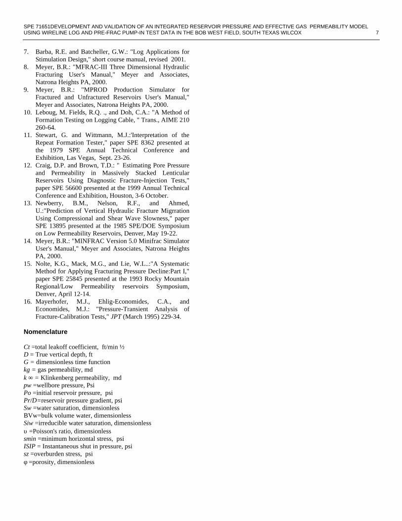
A model for estimating effective permeability to gas wasdeveloped with the integration of wireline log, net overburdenstressed (NOB) Klinkenberg corrected core data, and well testeffective permeability data.5,7 The permeability model usesporosity and a Modified Simandoux water saturation estimateas key inputs. The base porosity model is calibrated to NOBKlinkenberg porosity, and the base model water saturation iscalibrated to core capillary pressure or Nuclear Magneticresonance data. The calibrated model is then used to processthe digital log data using the PETCOM PC-based log analysisprogram. 6 A comparison of model results with thesecalibration standards is shown in Fig. 1. The in-situ stressdistribution is estimated using a correlation between shalevolume and Poisson's ratio, with additional inputs ofoverburden gradient and pore pressure.7 Shale volumes arecalibrated to core X-ray diffraction data, and dipole sonic dataare subjected to a rigorous quality control process. The in-situstress estimates are then calibrated to pre-frac pump-in testdata.7 The calibrated inputs are entered into the MFRAC-III P-3D hydraulic fracture simulator to predict propped fracturedimensions.8 This propped fracture geometry is then enteredinto a single phase reservoir simulator to obtain a post fracproduction rate.9 Bottomhole flowing pressure can beobtained for all zones directly from a wireline or slicklineconveyed production log. Reservoir pressure, however, isnormally obtained from individual zone transient pressuretests. This process can be costly and time consuming inmultiple zone environments. In the Bob West Field Wilcoxthere are often as many as eight separate fracture treatmentsrequired to effectively drain the recoverable gas in a singlewellbore. While it is relatively straightforward to perforatethe lowest zone and obtain a conventional pre-frac transientpressure test in that zone, the procedure becomes significantlymore complex for the subsequent zones. As a resultconventional transient pressure tests are rarely obtained inmultiple zone Wilcox completions in the Bob West Field.

Wireline Formation Pressure Tests

A practical alternative to obtain reservoir pressure is anopenhole wireline formation tester. These tools have beenavailable in various forms in the industry since 1955.10, 11 Thetool is run in the hole on electric line and positioned acrossfrom the zone of interest. A pad assembly is forced up againstthe sand face by an opposed piston and a seal is obtainedaround the probe. A pre-test chamber is opened up andformation fluid is allowed to flow into the pre-test chamber.Once reservoir pressure is either reached or extrapolated thetool is retracted and the next zone tested. The time requiredfor each test is a function of reservoir permeability andpressure, however in the study area Well 1 had 24 testsconducted in a six hour period, Well 2 had 40 tests conductedin a five hour period and Well 3 had 58 tests conducted in aten hour period. This is an average of 10 minutes per test. Inthe majority of cases adequate flow was obtained to either

measure directly or extrapolate a stabilized reservoir pressure.Conventional wisdom among many operators dictates thatwireline formation testers are not useful in low permeabilitygas zones.12 This is clearly not the case in the Bob WestLopeno Wilcox field.

Relationship Between Reservoir Pressure and In-situStress

Reservoir pressure is a key component of the minimumhorizontal in-situ stress estimate. Additional inputs requiredare overburden gradient, Poisson's Ratio, and a calibrationcomponent. The most commonly used relationship is:7,13

(1) Smin/D = sz/D * (ν/1-ν) + Pr/D* (1-(ν/(1-ν)) + Pext

Where:Smin/D = closure stress gradient (psi/ft)

sz/D = overburden gradient (psi/ft)ν = Poisson's ratioPr/D = pore pressure gradient (psi/ft)Pext = calibration component (psi/ft)

The calibration for the above equation is done using a pre-fracpump in test that measures closure pressure. If closure is notobtained a match is needed between the field ISIP andpressure decline and the predictions made using a P-3Dhydraulic fracture simulator.7

Overburden Gradient

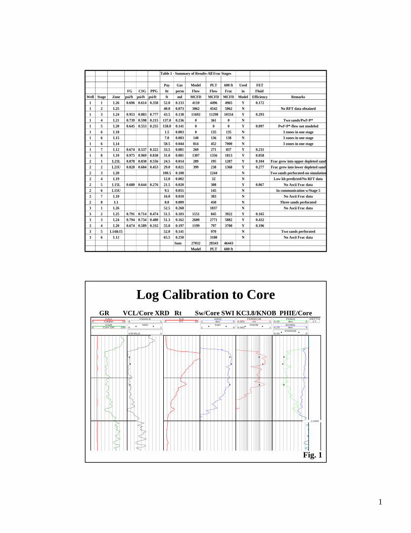
The input of overburden gradient can be directly calculatedfrom the bulk density log data.13 In the study area this variesfrom 1.06 psi/ft at 8000 ft TVD to 1.074 psi/ft at 12000 ftTVD. It can be estimated from an empirical correlation withdepth using the following relationship:

(2) sz/D= 0.0303Ln(D) + 0.7895

Where:

sz = overburden pressure psiD= True vertical depth ft

A graphical relationship between TVD and overburden for thefield is shown in Fig. 2. This narrow range of values at theobjective depth will be a consideration in subsequentempirical calculations.

Poisson's Ratio

The input of Poisson's ratio is initially obtained from a fullwave (one that measures both P and S wave) sonic tool.13 InSouth Texas this can only be obtained from a Dipole Sonictype tool due to the high shear transit times.7 Once the dipole

SPE 71651DEVELOPMENT AND VALIDATION OF AN INTEGRATED RESERVOIR PRESSURE AND EFFECTIVE GAS PERMEABILITY MODELUSING WIRELINE LOG AND PRE-FRAC PUMP-IN TEST DATA IN THE BOB WEST FIELD, SOUTH TEXAS WILCOX 3

data has been acquired, subsequent wells can use a shalevolume to Poisson's correlation to estimate this parameter.7 Inthe development of a relationship it is important to use onlydipole data that has high coherency or semblance (greater than85% is preferred).7 In a review of numerous dipole sonicsonly relatively small percentage of the total interval loggedcontained coherent data. Once the coherent data is identified, acorrelation can usually be obtained between the dipole sonicPoisson's ratio and an empirical Poisson's based on shalevolume. In the Bob West Field the relationship used was:

(3) ν = 0.20 + (0.17*Vclay)

Where:

Vclay = clay volume from GR or NPHI-DPHI

From the above relationship a shale free zone would have aPoisson's ratio of 0.20. The majority of the productive sandshave between 5% and 10% clay in the highest qualityreservoir based on Xray diffraction analyses. These Vclayvalues result in a Poisson's ratio range of between 0.21 and0.23. This narrow variation in the higher quality reservoir rockwill be a consideration in subsequent empirical correlations.Shales can have values as high as 0.37, and siltstones varybetween the two extremes. The values used for gamma rayclean and shale should be adjusted so that clean zones have aminimum of 5% Vclay and shales not more than 100%. Analternative clay volume relationship to use involves usingeither an apparent grain density from the density and neutronlogs or the difference between the neutron and densityporosity. This equation should be limited to a minimum of5% Vclay as well to accommodate zones with densitycrossover.

Calibration Component Pext

The calibration component (Pext) can only be obtained afterall of the other inputs are compiled and used to estimate stress.This includes reservoir pressure, as without the reservoirpressure input two unknowns exist with only a single inputavailable. An initial value of zero is assumed in the pre-fracpump-in test 3D frac model analysis. Once the pump-in testdata are compared to the model prediction a linear gradientshift is made to match the two pressures.7 This gradientbecomes the Pext function. In the study area a Pext of 0.085was determined to apply in all zones. A match between fieldpressures and the MFRAC-III 3-D model pressures using thisPext is shown in Fig. 3. This is important in that the valuebecomes more than a "fudge factor" when it is found to repeatconsistently in all zones. In the case of Well 1 excellent pre-frac pump in test pressure matches were obtained in all eightstages using this single value. This consistency is also animportant issue in then subsequent empirical correlationbetween reservoir pressure and pre-frac pump-in test pressureestimates.

Empirical Correlation Technique

Once the overburden gradient, ν, and Pext terms areestablished, equation (1) can be used to estimate reservoirpressure using an input of closure pressure. Craig and Brown(1999) presented a study in the Mesaverde where reservoirpressure was estimated from closure stress using a derivativeof Eq. 1.12 A review of the terms involved in the Wilcox,however, suggest that a simpler technique may be applied.The overburden gradient varies only slightly as a function ofdepth, and the Pext function was determined to be veryconsistent. While Poisson's ratio varies significantly betweenthe perforated sands and the adjacent shales there is relativelylittle change within the cleanest sands themselves. Theremaining term in the equation is reservoir pressure. Sincethis was measured using the wireline formation tester, all ofthe components are present to perform a simple empiricalcorrelation between pre-frac pump in test pressures andmeasured reservoir pressures.

Empirical Correlation Procedures

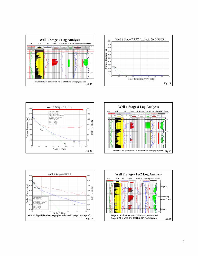
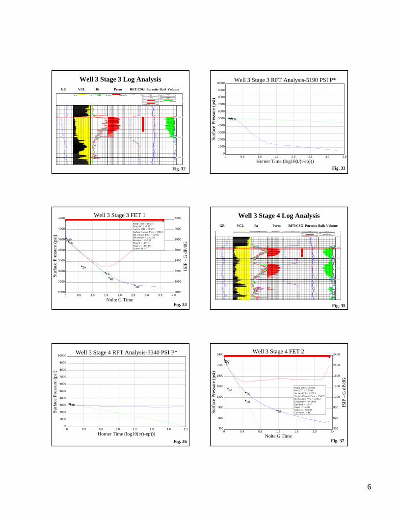
In the study area there were three wells analyzed in detail.Well 1 had eight frac stage intervals, Well 2 had eight fracstage intervals, and Well 3 had six frac stage intervals. A totalof 22 pre-frac pump-in tests (hereafter referred to as FETtests) were conducted from the three wells. The three wellsalso contained 122 wireline formation pressure tests.Openhole wireline density, neutron, gamma ray, andresistivity data were available for all three wells. Netoverburden stressed Klinkenberg corrected core permeabilitieswere available on all three wells. Zones with large or multipleperforated intervals were not analyzed. In several cases thedigital pump-in test data were not available, and in one case anRFT test was not successful in a zone where a pump-in testwas taken. The RFT pressure data was analyzed using aHorner plot analysis in the MINFRAC minifrac pressureanalysis program.14 The pre-frac pump-in tests were alsoanalyzed using the MINFRAC program using the Nolte "G"function and ISIP-x dp/dx derivative outputs.15 Estimatesobtained for each zone of ISIP and closure pressure. Elevendata points were obtained with quality RFT and pre-fracpump-in test results. Table 1 lists all stages in all wells witheither the results of the tests or an explanation why the stagewas not included in the empirical correlation. There was noattempt to exclude data points that did not fit the model unlessthere was a valid reason the data would not provide a uniquesolution. The PETCOM log analysis, MINFRAC RFT Hornerplots, and MINFRAC FET plots are displayed for all 11 zonesin Figs. 4 to 37.

Empirical Correlation Results

A strong correlation existed between measured reservoirpressure from the wireline formation tester and pre-frac pump-


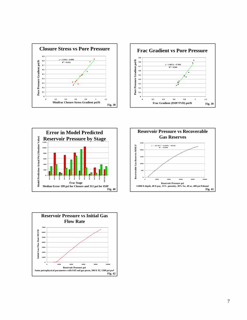
closure stress. There was a 0.9161 correlation coefficientbetween closure stress gradient and reservoir pressuregradient. The data and the linear regression line can be seen inFig. 38. The correlation between fracture gradient(ISIP/TVD) was even higher, with a 0.944 correlationcoefficient between the frac gradient and reservoir pressure.This data is shown in Fig. 39.

The relationships established were:

(5) Pr/D = 1.6012*ISIP/D- 0.7846 R2 = 0.944

(6) Pr/D = 1.3261* smin/D - 0.4688R2 = 0.9161

Where:Pr/D = Pore pressure gradient (psi/ft)ISIP/D = Frac gradient (psi/ft)Smin/D = Closure stress gradient (psi/ft)

Reservoir Pressure vs Recoverable Reserves

There was an average error of 0.0218 psi/ft in reservoirpressure between the best fit equation using closure stress asan input and 0.0282 psi/ft using the ISIP derived reservoirpressure. The error range was .003 psi/ft to 0.109 psi/ft usingclosure stress as an input and 0.007 psi/ft to 0.08 psi/ft usingthe frac gradient. To determine if this error is acceptable asensitivity between reservoir pressure and both volumetric gasreserves and initial gas rate was evaluated. Using reservoirproperties of 40 ft of pay, 15% porosity, 30% Sw, 40 acredrainage, and 11000 ft depth; recoverable gas at originalconditions would be 2257 MMCF. An error of 0.05 psi/ft inthis estimate (reducing the pore pressure from 0.80 psi/ft to0.75 psi/ft) would reduce the recoverable reserves to 2174MMCF. A reduction of 0.10 psi/ft to 0.70 psi/ft would reducethe recoverable reserves to 2085 MMCF. If the pressure isreduced to the average from all RFT tests of 0.36 psi/ft,however, the recoverable reserves are reduced to 1180MMCF. Fig. 41 is a plot of the relationship between reservoirpressure and recoverable reserves for the above reservoirproperties. Considering the range of observed reservoirpressures of 0.15 psi/ft to 0.82 psi/ft the range of expectedrecoveries for zones with similar petrophysical characteristicsis significant, with a range of 466 MMCF to 2257 MMCFbased on pressure alone.

Reservoir Pressure vs Initial Gas Rate

A similar sensitivity analysis can be done between reservoirpressure and expected gas flow rate using the beforementionedreservoir properties and assuming a permeability to gas of0.05md and a propped fracture half length of 500 ft. A 1500psi flowing sandface pressure was assumed as well. Areduction in reservoir pressure from 0.80 psi/ft to 0.75 psi/ftresults in an initial rate reduction from 6.6 MMCFD to 6.2

MMCFD. With a maximum error of 0.1 psi/ft the rate dropsto 5.8MMCFD. If the average RFT reservoir pressure of 0.36psi/ft is used the initial flow rate drops to 2.45 MMCFD. Fig.42 is a plot of the relationship between reservoir pressure andinitial gas rate for the above reservoir properties. Within therange of observed pressures in the three well dataset the initialflow rates vary from 0.153 MMCFD at 0.15 psi/ft to 6.6MMCFD at 0.80 psi/ft for zones with identical petrophysicalproperties.

While all single zone stages with quality RFT and FET datawere included in the statistical comparison, one zone wasexcluded with good quality data. Well 2 Stage 6 had asignificantly higher closure stress gradient than the pre-fracRFT test would suggest (Well 2 Stage 6). It had a 0.58 psi/ftclosure stress gradient with a 0.1763 psi/ft pore pressureobserved with the RFT. The model would have predicted a0.312 pore pressure gradient based on this closure stress.Upon closer review it was observed that there was a 14 ftsiltstone between the stages and subsequent frac modelingindicated that the Stage 5 frac should have grown into Stage 6.The initial pressure observed in Stage 6 would have thus beenelevated over the pressure observed before the frac treatmentswith the RFT.

Use of Closure Stress Gradient vs Frac Gradient

The superior correlation between ISIP and reservoir pressurewas not expected, as the ISIP value is the product of bothclosure stress and net fracture pressure generated during thepump-in period. A comparison of closure stress to ISIPindicated a range of values between 50 and 1500 psi, with anaverage net pressure of 733 psi. Another variable in thecomparison was the calculation accuracy of the ISIP andclosure stress. The ISIP value can generally be calculatedwith minimal variability, while the closure stress estimate isnot always clear in all cases. Even with the fairly rigoroustechnique used the first inflection point observed in the closureanalysis is not always indicative of the minimum horizontalclosure stress. It is recommended, however, that closurestress be used as the primary input with the fracture gradientused as a "quicklook" technique in areas where pre-frac pumpin net pressures are similar. Another possibility is to minimizethe pump in test volumes on an initial pump in test to obtainfracture gradient and closure stress then increase the volumeon a second test to calculate fluid efficiency and optimum padvolume.

Implications of Model Results

With the strong correlations obtained between measuredreservoir pressures and pre-frac pump-in test pressures, onfuture wells where measured pressures are not available thereservoir pressure predicted from the pump-in test can beused. These pressures can be used along with the permeabilityinputs discussed next to predict formation deliverability.


These pre-frac pump-in tests can be performed on all wells ina relatively short period of time at minimal additional cost.

Integration of Results with Permeability Model

With a solid base to estimate reservoir pressure, the nextcomponent of the integrated reservoir performance model iseffective gas permeability. The model that ha provided thebest results in the Wilcox is a modified Coates-Denooequation using log derived effective porosity and bulk volumewater:5,7

(7) kg = ((C*φ e 2*((φ e - BVw)/ BVw)))2

WhereC = Calibration factorkg = Effective gas permeabilityφ e = Effective porosityBVw = Modified Simandoux (Sw*φ e)

The calibration factor "C" was initially established with acalibration to net overburden stressed Klinkenberg correctedcore permeabilities. In the Bob West field a value of 3.8 hasprovided a reasonable estimate of effective gas permeability aswell when the calibrated permeability-thickness is comparedto transient pressure test permeability thickness. Acomparison of log derived permeability values with NOBKlinkenberg core permeabilities is shown in Fig. 1.

Several diagnostic techniques have been presented in otherwork that use the pressure decline data to estimate effectivepermeability.12,16 The techniques in these references involvedusing pressure decline analysis of the pre-frac FET. Inaddition to these techniques, the RFT analysis on Well 1provided a drawdown permeability that was generally in thesame order of magnitude as the log derived values. Whilethese dynamic permeability measurement techniques haveproduced good results in other areas, no attempt was made toestimate permeability from the pump-in test data in this study.The log derived techniques provided acceptable results andthese results were available in a more timely fashion in thecompletion process. More work is recommended to integratethe pump-in test and wireline formation tester techniques andthe log derived techniques to reduce the errors involved inusing only a single technique.

Fracture Geometry Predictions

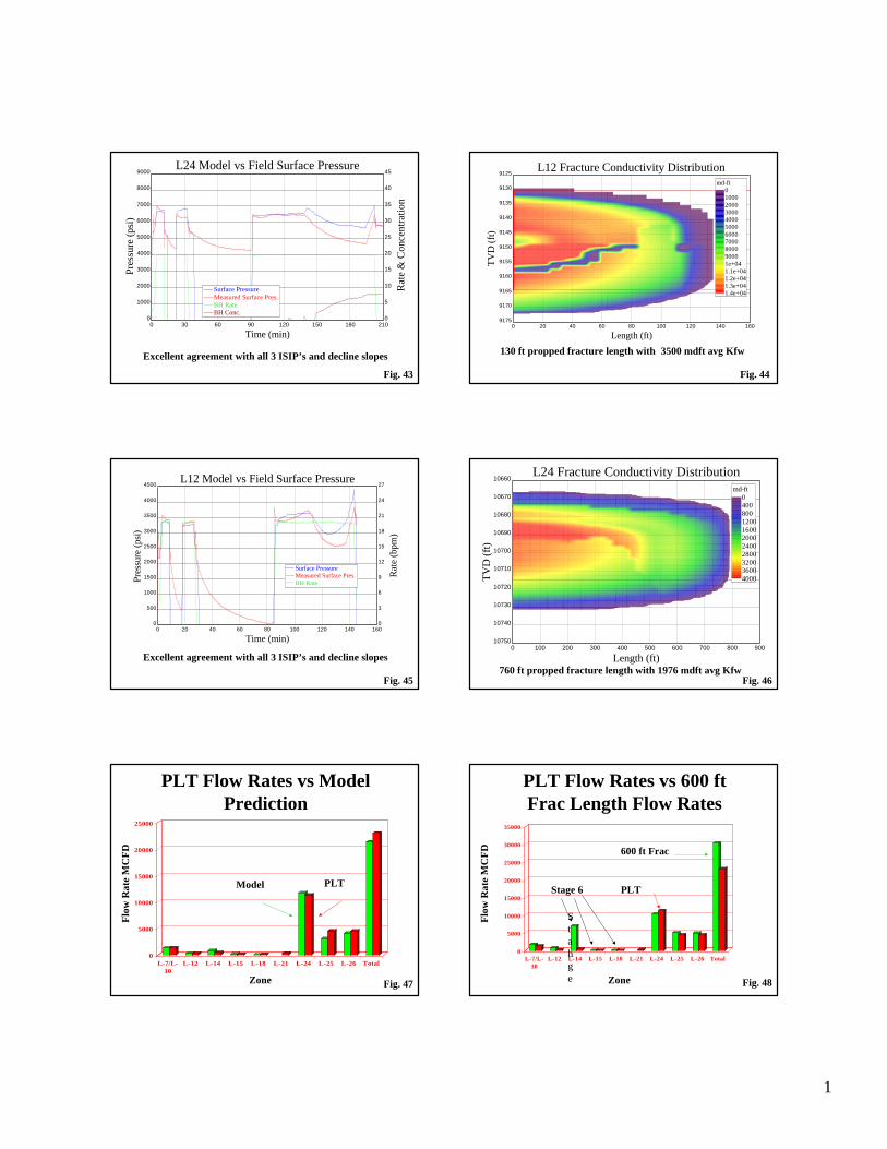
The stress profiles calibrated with pre-frac pump-in tests wereloaded into the MFRAC-III P3D hydraulic fracture simulator.The simulator was run and estimates were provided of fracturelength and conductivity. The results of the fracture simulationsfor two of the zones are shown in Figs. 43-46. A low reservoirpressure zone was presented as well as a virgin zone toillustrate the different geometries from the same basic fracdesign. These estimates were then loaded into the MPROD

production simulator along with the reservoir pressure andpermeability data to predict production.

Young's Modulus Estimation

While not part of the stress estimation process, an input forYoung's modulus is required for the 3D frac simulation. Theequation for calculating Young's modulus from wireline logdata is:

(8) E = 2*G*(1+ ν)(9) Gm = 13400*(ρb/∆TS^2)

Where:E = Dynamic Young's Modulus (psi x E6)Gm= Shear Modulus (psi x E6)ρb = Bulk density g/cc∆TS = Shear transit time msec/ft

Without a measured Dipole sonic the required input of sheartransit time is not available. With compressional sonic data(∆TC) an estimate of ∆TS can be made from a back-calculation of the shear/compressional ration from theempirical Poisson's ratio. The equation for this is:

(10) SCR = (12.105*ν^2)-(3.1833*ν)+1.7466

where:

SCR=∆TS/∆TC ratio

In cases where a compressional sonic is not available acorrelation can be usually made in the Wilcox between ∆TCand Φn (neutron porosity). This can be done with a linearregression over the Wilcox interval, and the equationdeveloped is only for the Bob West field. The relationshipdeveloped is:

(11) ∆TC = 210*Φn+38.7

where:

Φn = Neutron sandstone porosity (NPHI) v/v

The correlation coefficient for this relationship was 0.88, thusit can be used with a reasonable level of confidence in thisfield.

Model Validation

Following the fracture treatment a production log was runacross all producing zones. This provided a measurement ofactual flowing wellbore pressure and an estimate of flow ratefrom each zone. In the case of Well 1 the model predictions


agreed well with the PLT results from all zones (Table 1 andFig. 47). The flow rate predicted from the integration of thereservoir model and 3D model frac geometry was 21.4MMCFD, compared to an actual flow rate of 23 MMCFD.0.36 MMCFD of the difference was from Stage 4 where theRFT pressure was estimated to be below the PLT Pwf and nomodel prediction was made. With this zone excluded themodel prediction was 94.3% of the actual flow rate. Anestimate was made with the model assuming a 600 ft fracturelength in all zones (Table 1 and Fig. 48). The predicted flowrate with this frac length was 30.3 MMCFD. The majority ofthis 7.2 MMCFD discrepancy was from an ineffectivecompletion in Stage 6 where an additional 6.5 MMCFDshould have been recovered with an effective frac treatment.Three zones were treated together in Stage 6 (L18, L15, andL14). The uppermost L14 zone had 99% of the kh and 91% ofthe volumetric reserves in that stage. The post frac PLTanalysis indicated that the zone was producing only 62.5% ofthe total flow rate from the three zones. While the L-14 wasproducing 452 MCFD, the zone should have produced 814MCFD with 0 skin and 7 MMCFD with a 600 ft frac length.A comparison of expected results with a 600 ft frac length inall zones is shown in Table 1. The lack of a good stimulationtreatment in the L14 resulted in a loss of over 6.5 MMCFD ofinitial rate and put the recovery of the 1.8 BCF of remainingreserves in that zone in question. The results for all of theother zones in Well 2 and Well 3 with adequate data for asimulation are included for comparison as well. Theagreement between the model prediction and actual measuredflow rates is also excellent in the other two wells.

Fracture Design Considerations

The FET fluid efficiencies varied from 6% to 43% among thevarious zones with the 30 lb linear gel system. This is clearlynot a situation where a "one size fits all" fracture design isappropriate. In several of the 3D frac simulations in zoneswith less than virgin pressure it appeared that "tip screenouts"occurred prior to the fracs reaching the 600 ft target fraclength. While tip screenouts are recommended in almost allcases for high permeability reservoirs, in low permeabilitythey should be used carefully if the tip screenout occurs priorto the target length being reached (Fig 49). There is apotential for lost production if the target length is not reached.The benefit of substantially increasing the conductivity at theexpense of length is questionable in low permeability. On thecost side, once the tip screenout begins there is often marginalbenefit to continuing the proppant schedule if the targetconductivity has been reached at the point of tip screenoutinitiation. With the high closure stresses involved in theWilcox premium proppants are used, and pumping largevolumes of excess proppant may also not be cost effective.

The lower fluid efficiencies in lower reservoir pressure zonesare driven by two primary factors. The first is the increasedclosure stress from the reduction in the PPG term in Eq. (Fig.50). In a typical Bob West Wilcox zone a reduction from a

0.82 virgin pore pressure gradient to a 0.65 PPG increases theconfining stress from 400 psi to 1600 psi. The majority of thefrac is contained in the permeable interval as confiningstresses increase. The second factor is the increased pressuredifferential between the fracture and the reservoir at reducedpressures. In many cases the job designs resulted in "tipscreenout" treatments due to excess fluid loss. In the higherreservoir pressure intervals fracture lengths were generallylonger due to increased fluid efficiency in spite of the reducedstress contrast. The principal culprit for shorter than optimumfrac lengths appeared to be insufficient pad volumes to dealwith the excessive leakoff encountered from reduced porepressure rather than significant height growth.

Conclusions

An integrated model has been developed for the Bob WestLopeno Wilcox field that provides for reasonable estimates ofpost-frac gas deliverability using readily available data. Thecritical input of reservoir pressure can be estimated fromrelatively simple pre-frac pump-in test analysis. Wireline logdata correlated to core and well test data can provide areasonable estimate of effective permeability to gas. Wirelinelogs calibrated to pump-in test data can also provide areasonable estimate of the minimum horizontal stressdistribution. From these readily available inputs a forecast offormation deliverability as a function of hydraulic fracturegeometry can be made. While the model is relatively simpleand economical to implement, it provides all of the necessaryinformation to determine the optimum stimulation design forany zone in the Bob West Lopeno Wilcox field.

References

1. Agarwal, R.G., Carter, R.D., and Pollock, C.B.:“Evaluation and Performance Prediction of LowPermeability Gas Wells Stimulated by Massive HydraulicFracturing,” JPT (March 1979) 362-72; Trans. AIME,267.

2. Cinco-Ley, H. and Samaniego-V., F.: “Transient-PressureAnalysis for Fractured Wells, JPT (Sept. 1981) 1641-66

3. Meng, H,Z. et al.: “Production Systems Analysis ofVertically Fractured Wells,” paper SPE 10842 presentedat the 1982 SPE/DOE Unconventional Gas RecoverySymposium, Pittsburgh, May 16-18

4. Meng, H.Z. and Brown, K. E.: “Coupling of ProductionForecasting Fracture Geometry Requirements, andTreatment Scheduling in the Optimum Hydraulic FractureDesign,” paper SPE 16435 presented at tbe 1987SPE/DOE Symposium on Low Permeabtilty Reservoirs,Denver, May 18-19.

5. Coates, G.R. and Denoo, S.:"The Producibility AnswerProduct," Schlumberger Technical Review 29, No. 2,June 1981, 55.

6. PETCOM Powerlog User's Manual, Petcom Inc., Dallas,Texas 1999.


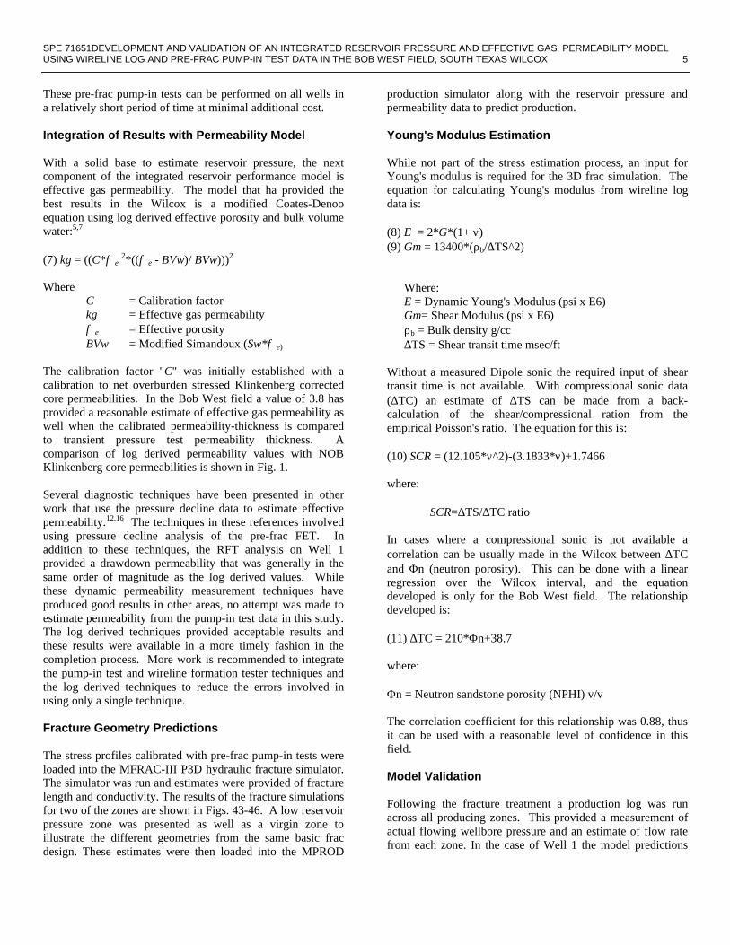
7. Barba, R.E. and Batcheller, G.W.: "Log Applications forStimulation Design," short course manual, revised 2001.

8. Meyer, B.R.: "MFRAC-III Three Dimensional HydraulicFracturing User's Manual," Meyer and Associates,Natrona Heights PA, 2000.

9. Meyer, B.R.: "MPROD Production Simulator forFractured and Unfractured Reservoirs User's Manual,"Meyer and Associates, Natrona Heights PA, 2000.

10. Leboug, M. Fields, R.Q. ., and Doh, C.A.: "A Method ofFormation Testing on Logging Cable, " Trans., AIME 210260-64.

11. Stewart, G. and Wittmann, M.J.:'Interpretation of theRepeat Formation Tester," paper SPE 8362 presented atthe 1979 SPE Annual Technical Conference andExhibition, Las Vegas, Sept. 23-26.

12. Craig, D.P. and Brown, T.D.: " Estimating Pore Pressureand Permeability in Massively Stacked LenticularReservoirs Using Diagnostic Fracture-Injection Tests,"paper SPE 56600 presented at the 1999 Annual TechnicalConference and Exhibition, Houston, 3-6 October.

13. Newberry, B.M., Nelson, R.F., and Ahmed,U.:"Prediction of Vertical Hydraulic Fracture MigrrationUsing Compressional and Shear Wave Slowness," paperSPE 13895 presented at the 1985 SPE/DOE Symposiumon Low Permeability Reservoirs, Denver, May 19-22.

14. Meyer, B.R.: "MINFRAC Version 5.0 Minifrac SimulatorUser's Manual," Meyer and Associates, Natrona HeightsPA, 2000.

15. Nolte, K.G., Mack, M.G., and Lie, W.L..:"A SystematicMethod for Applying Fracturing Pressure Decline:Part I,"paper SPE 25845 presented at the 1993 Rocky MountainRegional/Low Permeability reservoirs Symposium,Denver, April 12-14.

16. Mayerhofer, M.J., Ehlig-Economides, C.A., andEconomides, M.J.: "Pressure-Transient Analysis ofFracture-Calibration Tests," JPT (March 1995) 229-34.

Nomenclature

Ct =total leakoff coefficient, ft/min ½D = True vertical depth, ftG = dimensionless time functionkg = gas permeability, mdk ∞ = Klinkenberg permeability, mdpw =wellbore pressure, PsiPo =initial reservoir pressure, psiPr/D=reservoir pressure gradient, psiSw =water saturation, dimensionlessBVw=bulk volume water, dimensionlessSiw =irreducible water saturation, dimensionlessυ =Poisson's ratio, dimensionlesssmin =minimum horizontal stress, psiISIP = Instantaneous shut in pressure, psisz =overburden stress, psiφ =porosity, dimensionless

1

Table 1 - Summary of Results-All Frac Stages

Pay Gas Model PLT 600 ft Used FET

FG CSG PPG ht perm Flow Flow Frac in Fluid

Well Stage Zone psi/ft psi/ft psi/ft ft md MCFD MCFD MCFD Model Efficiency Remarks

1 1 L26 0.696 0.614 0.358 52.0 0.133 4110 4496 4965 Y 0.172

1 2 L25 40.0 0.073 3062 4542 5062 N No RFT data obtained

1 3 L24 0.953 0.883 0.777 43.5 0.138 11692 11298 10334 Y 0.293

1 4 L21 0.739 0.598 0.215 137.0 0.236 0 361 0 N Two sands/Pwf=P*

1 5 L20 0.645 0.553 0.255 158.0 0.141 0 0 0 Y 0.097 Pwf=P*-flow not modeled

1 6 L18 1.5 0.003 0 135 135 N 3 zones in one stage



1 7 L12 0.674 0.537 0.322 33.5 0.081 269 271 837 Y 0.231

1 8 L10 0.975 0.969 0.838 31.0 0.081 1307 1356 1813 Y 0.058

2 1 L21L 0.878 0.830 0.556 24.5 0.014 289 195 1287 Y 0.104 Frac grew into upper depleted sand

2 2 L21U 0.828 0.684 0.453 29.0 0.021 399 238 1368 Y 0.277 Frac grew into lower depleted sand

2 3 L20 100.5 0.108 1244 N Two sands perforated-no simulation

2 4 L19 12.0 0.002 32 N Low kh predicted/No RFT data

2 5 L15L 0.680 0.644 0.276 21.5 0.020 308 Y 0.067 No Ascii Frac data

2 6 L15U 9.5 0.055 145 N In communication w/Stage 5

2 7 L10 16.0 0.010 383 N No Ascii Frac data

2 8 L1 8.0 0.009 450 N Three sands perforated


3 2 L25 0.791 0.714 0.474 51.5 0.103 1151 845 3922 Y 0.165

3 3 L24 0.794 0.734 0.480 51.3 0.162 2600 2771 5882 Y 0.432

3 4 L20 0.674 0.589 0.332 55.0 0.197 1199 797 3700 Y 0.196

3 5 L14&15 52.0 0.141 970 N Two sands perforated


Sum 27032 28343 46443

Model PLT 600 ft

Log Calibration to CoreGR VCL/Core XRD Rt Sw/Core SWI KC3.8/KNOB PHIE/Core

Fig. 1

CALICaliper6 16

CGRCorr GR0 100

VSHALE 0 1

♦ ♦XRD

0 1

VSHALE 1

ILDRT0 30

SWQdec1 0

♦ ♦SWI

1 0

PERMC38v/v0.001 1

♦ ♦KNOB

0.001 1

PHIEQdec0.25 0

BVWQdec0.25 0

♦ ♦PHINOB 0.25 0

DEPTHFT

♦

♦

♦

♦

♦

♦

♦

♦

♦

♦

♦

♦

11400

1

Bob West Field Overburden Gradientvs True Vertical Depth

y = 0.0303Ln(x) + 0.7895

R2 = 1

1.01

1.02

1.03

1.04

1.05

1.06

1.07

1.08

0 2000 4000 6000 8000 10000 12000 14000

TVD ft

OB

G p

si/f

t

Fig. 2Excellent agreement with all 3 ISIP’s and decline slopes

Well 1 Stage 1 3D Model vs Field Surface Pressure

0 30 60 90 120 150 180 210

Time (min)

0

1000

2000

3000

4000

5000

6000

7000

8000

9000

Pres

sure

(ps

i)

0

1

2

3

4

5

6

7

8

9

Con

cent

ratio

n (l

bm/g

al)

Surface PressureMeasured Surface Pres.BH Conc.

Fig. 3

Well 1 Stage 1 Log AnalysisGR VCL Rt Perm RFT/CSG PLT/RA Porosity Bulk Volume

52 ft of 14% porosity/29.4% Sw/0.133md perm/kh 6.92 mdft Fig.4

CALIIN6 16

GRGAPI0 150

GRCapi0 150

VCLQdec0 1

0 VCLQ

VCLQ 1

AO10OHM.0 20

AF90OHM.0 20

♦ ♦RFTMOB

0.001 1

PERMC38v/v0.001 1

0.001 PERMC38

♦ ♦RFTPPG

0 1

PRNDEN 0.2 0.4

PPGCURV1v/v0 1

PLTMMCF 0 1000

TRACER 10 0

0 PLTMMCF

RHOBG/CM2.16 2.65

NPHIFT3/0.3 0

RHOB NPHI

BVWFINALv/v0.25 0

DPHIdec0.25 0

BVWDEC0.25 0

DEPTHFT

♦ ♦

L2611000

11050

Well 1 Stage 1 RFT Analysis-3987 PSI P*

0 0.3 0.6 0.9 1.2 1.5 1.8 2.1

Horner Time (log10(t/(t-ep)))

-500

0

500

1000

1500

2000

2500

3000

3500

4000Su

rfac

e Pr

essu

re (

psi)

1A1B

Fig. 5

Well 1 Stage 1 FET

0 0.2 0.4 0.6 0.8 1.0 1.2 1.4 1.6

Nolte G Time

900

1200

1500

1800

2100

2400

2700

3000

Surf

ace

Pres

sure

(ps

i)

900

1200

1500

1800

2100

2400

2700

3000

ISIP

- G

dP/

dG

ISIP

TC

1A

1B

2A

2B

Pump Time = 40.764Delta TC = 10.117Surface ISIP = 2828.7Surface Closure Pres. = 1923.1BH Closure Pres. = 4089.7Efficiency* = 0.17175Residual = 166.37Slope 1 = -2180.6Slope 2 = -1212.5Current Pt. = TC

Fig. 6

Well 1 Stage 3 Log AnalysisGR VCL Rt Perm RFT/CSG PLT/RA Porosity Bulk Volume

43.5 ft of 13.9% porosity/28% Sw/0.138 md average gas permFig. 7

CALIIN6 16

GRGAPI0 150

GRCapi0 150

VCLQdec0 1

0 VCLQ

VCLQ 1

AO10OHM.0 20

AF90OHM.0 20

♦ ♦RFTMOB

0.001 1

PERMC38v/v0.001 1

0.001 PERMC38

♦ ♦RFTPPG

0 1

CSG 0.5 1

PPGCURV1v/v0 1

PLTMMCF 0 1000

TRACER 10 0

0 PLTMMCF

RHOBG/CM2.16 2.65

NPHIFT3/0.3 0

RHOB NPHI

BVWFINALv/v0.25 0

DPHIdec0.25 0

BVWDEC0.25 0

DEPTHFT

♦

♦

♦

♦

L24

10700

10750

2


0 0.3 0.6 0.9 1.2 1.5 1.8 2.1


0

1000

2000

3000

4000

5000

6000

7000

8000

9000

10000

Surf

ace

Pres

sure

(psi

) 1A1B

Fig. 8

Well 1 Stage 3 FET 2

0 0.3 0.6 0.9 1.2 1.5 1.8

Nolte G Time

4200

4400

4600

4800

5000

5200

5400

5600

5800

Surf

ace

Pres

sure

(ps

i)

4200

4400

4600

4800

5000

5200

5400

5600

5800

ISIP

- G

dP/

dG

ISIP

TC

1A

1B

2A

2B

Pump Time = 32.253Delta TC = 17.832Surface ISIP = 5484.7Surface Closure Pres. = 4733.3BH Closure Pres. = 6900Efficiency* = 0.29277Residual = 70.617Slope 1 = -907.5Slope 2 = -720.08Current Pt. = TC

Fig. 9

Well 1 Stage 5 Log Analysis

158 ft of 12.1% porosity/29.6% Sw/0.141 md average gas perm

CALIIN6 16

GRGAPI0 150

GRCapi0 150

VCLQdec0 1

0 VCLQ

VCLQ 1

AO10OHM.0 20

AF90OHM.0 20

♦ ♦RFTMOB

0.001 1

PERMC38v/v0.001 1

0.001 PERMC38

♦ ♦RFTPPG

0 1

CSG 0.5 1

PPGCURV1v/v0 1

PLTMMCF 0 1000

TRACER 10 0

0 PLTMMCF

RHOBG/CM2.16 2.65

NPHIFT3/0.3 0

RHOB NPHI

BVWFINALv/v0.25 0

DPHIdec0.25 0

BVWDEC0.25 0

DEPTHFT

♦

♦

♦

♦

L20

9950

10000

10050

10100

GR VCL Rt Perm RFT/CSG PLT/RA Porosity Bulk Volume

Fig. 10


0 0.3 0.6 0.9 1.2 1.5 1.8 2.1


0

1000

2000

3000

4000

5000

6000

7000

8000

9000

10000

Surf

ace

Pres

sure

(ps

i)

1A 1B

Fig. 11


0 0.2 0.4 0.6 0.8 1.0 1.2

Nolte G Time

0

300

600

900

1200

1500

1800

2100

2400

Surf

ace

Pres

sure

(ps

i)

0

300

600

900

1200

1500

1800

2100

2400

ISIP

- G

dP/

dG

ISIP

TC

1A

1B2A

2B

Pump Time = 23.339Delta TC = 2.8026Surface ISIP = 2042Surface Closure Pres. = 1130.1BH Closure Pres. = 3296.7Efficiency* = 0.097103Residual = 624.01Slope 1 = -4805.8Slope 2 = -3054.3Current Pt. = TC

Fig. 12


Upper zone (L14) received only minor stimulation in multiple zone frac


Fig. 13

CALIIN6 16

GRGAPI0 150

GRCapi0 150

VCLQdec0 1

0 VCLQ

VCLQ 1

AO10OHM.0 20

AF90OHM.0 20

♦ ♦RFTMOB 0.001 1

PERMC38v/v0.001 1

0.001 PERMC38

♦ ♦RFTPPG 0 1

CSG 0.5 1

PPGCURV1v/v0 1

PLTMMCF 0 1000

TRACER 10 0

0 PLTMMCF

RHOBG/CM2.16 2.65

NPHIFT3/0.3 0

RHOB NPHI

BVWFINALv/v0.25 0

DPHIdec0.25 0

BVWDEC0.25 0

DEPTHFT

♦

♦

♦

♦

♦

♦

♦

♦

L14

L15

L18

9350

9400

9450

9500

9550

9600

9650

3


CALIIN6 16

GRGAPI0 150

GRCapi0 150

VCLQdec0 1

0 VCLQ

VCLQ 1

AO10OHM.0 20

AF90OHM.0 20

♦ ♦RFTMOB 0.001 1

PERMC38v/v0.001 1

0.001 PERMC38

♦ ♦RFTPPG 0 1

CSG 0.5 1

PPGCURV1v/v0 1

PLTMMCF 0 1000

TRACER 10 0

0 PLTMMCF

RHOBG/CM2.16 2.65

NPHIFT3/0.3 0

RHOB NPHI

BVWFINALv/v0.25 0

DPHIdec0.25 0

BVWDEC0.25 0

DEPTHFT

♦

♦

♦

♦

L12

9100

9150

9200


33.5 ft of 16.6% porosity/38.4% Sw/0.081 md average gas permFig. 14


0 0.3 0.6 0.9 1.2 1.5 1.8 2.1 2.4


0

1000

2000

3000

4000

5000

6000

7000

8000

9000

10000

Surf

ace

Pres

sure

(ps

i)

1A1B

Fig. 15


0 0.2 0.4 0.6 0.8 1.0 1.2 1.4 1.6

Nolte G Time

0

400

800

1200

1600

2000

2400

2800

Surf

ace

Pres

sure

(ps

i)

0

400

800

1200

1600

2000

2400

2800

ISIP

- G

dP/

dG

ISIP

TC

1A

1B

2A

2B

Pump Time = 28.417Delta TC = 10.765Surface ISIP = 2139.5Surface Closure Pres. = 887.65BH Closure Pres. = 3054.3Efficiency* = 0.2309Residual = 70.505Slope 1 = -1980.2Slope 2 = -922.19Current Pt. = ISIP

Fig. 16


CALIIN6 16

GRGAPI0 150

GRCapi0 150

VCLQdec0 1

0 VCLQ

VCLQ 1

AO10OHM.0 20

AF90OHM.0 20

♦ ♦RFTMOB 0.001 1

PERMC38v/v0.001 1

0.001 PERMC38

♦ ♦RFTPPG 0 1

CSG 0.5 1

PPGCURV1v/v0 1

PLTMMCF 0 1000

TRACER 10 0

0 PLTMMCF

RHOBG/CM2.16 2.65

NPHIFT3/0.3 0

RHOB NPHI

BVWFINALv/v0.25 0

DPHIdec0.25 0

BVWDEC0.25 0

DEPTHFT

♦ ♦

L108900

8950

9000


31 ft of 13.9% porosity/38.4% Sw/0.081 md average gas perm Fig. 17


0 0.2 0.4 0.6 0.8 1.0 1.2

Nolte G Time

4560

4600

4640

4680

4720

4760

4800

4840

Surf

ace

Pres

sure

(psi

)

4560

4600

4640

4680

4720

4760

4800

4840

ISIP

- G

dP/

dG

ISIP

TC

1A

1B2A

2B


RFT no digital data-hardcopy plot indicated 7506 psi 0.819 psi/ft

Fig. 18

Well 2 Stages 1&2 Log AnalysisGR VCL Rt Perm RFT/CSG Porosity Bulk Volume

RHOMANDg/cc2.5 3

EHGRGAPI0 200

VCLGRdec0 1

0 VCLGR

VCLGR 1

AO10OHM.0 40

AF90OHM.0 40

PERMC38v/v0.001 1

♦ ♦KNOB 0.001 1

0.001PERMC38

♦ ♦RFTPPG 0 1

CSG 0.6 1.1

PPGCURVT 0 1

HRHOG/CM2.16 2.65

HNPOFT3/0.3 0

PERFSv/v10 0

BVWFINALv/v0.25 0

BVWDEC0.25 0

HDPHIdec0.25 0

TVDFT

♦

♦

♦

♦

♦

♦

♦

♦

♦

♦

♦

♦

♦

♦

♦

♦

♦

♦

♦

♦

♦

L21

10500

10550

10600

10650

Stage 2

Perfs onlyAfter Fracs

Stage 1

Fig. 19

Stage 1 24.5 ft of 9.0% PHIE/0.293 Sw/0.012 mdStage 2 27 ft of 12.1% PHIE/0.219 Sw/0.164 md

4


0 0.2 0.4 0.6 0.8 1.0 1.2 1.4 1.6


0

1000

2000

3000

4000

5000

6000

7000

8000

9000

10000

Surf

ace

Pres

sure

(ps

i)

1A1B

Fig. 20

Well 2 Stage 1 FET

0 0.4 0.8 1.2 1.6 2.0 2.4 2.8

Nolte G Time

3400

3600

3800

4000

4200

4400

4600

4800

Surf

ace

Pres

sure

(ps

i)

3400

3600

3800

4000

4200

4400

4600

4800

ISIP

- G

dP/

dG

ISIP

TC

1A

1B2A

2B

Pump Time = 9.1649Delta TC = 1.2014Surface ISIP = 4656.4Surface Closure Pres. = 4144.1BH Closure Pres. = 6310.7Efficiency* = 0.10439Residual = 1047.2Slope 1 = -5506Slope 2 = -1207Current Pt. = TC

Fig. 21


0 0.4 0.8 1.2 1.6 2.0 2.4 2.8


0

1000

2000

3000

4000

5000

6000

7000

8000

9000

10000

Surf

ace

Pres

sure

(ps

i)

1A1B

Fig. 22

Well 2 Stage 2 FET

0 0.4 0.8 1.2 1.6 2.0 2.4

Nolte G Time

2700

3000

3300

3600

3900

4200

4500

4800

Su

rfac

e P

ress

ure

(ps

i)

2700

3000

3300

3600

3900

4200

4500

4800

ISIP

- G

dP/

dG

ISIP

TC

1A

1B

2A

2B


Fig. 23

Well 2 Stages 5&6 Log Analysis

CALIIN6 16

GRGAPI0 150

( GRC )0 150

VCLGRdec0 1

0 VCLGR

VCLQ 1

AO10OHM.0 20

AF90OHM.0 20

♦ ♦( RFTMOB )0.001 1

PERMC38v/v0.001 1

0.001 PERMC38

♦ ♦RFTPPG 0 1

CSG 0.5 1

PPGCURVF 0 1

( PLTMMCF )0 1000

( TRACER )10 0

0 PLTMMCF

RHOBG/CM2.16 2.65

NPHIFT3/0.3 0

RHOB NPHI

BVWFINALv/v0.25 0

DPHIdec0.25 0

BVWDEC0.25 0

DEPTHFT

♦

♦

♦

L15

10050

10100

10150

GR VCL Rt Perm RFT/CSG Porosity Bulk Volume

Fig. 24Stage 5 21.5 ft of 14.4% PHIE/0.423Sw/0.020 mdStage 6 9.5 ft of 15.6% PHIE/0.356 Sw/0.055 md

Well 2 Stage 5 RFT Analysis-2586 psi P*

0 0.2 0.4 0.6 0.8 1.0 1.2


1700

1800

1900

2000

2100

2200

2300

2400

2500

2600

Surf

ace

Pres

sure

(ps

i)

1A

1B

Fig. 25

5

Well 2 Stage 5 FET

0 0.05 0.10 0.15 0.20 0.25 0.30 0.35 0.40 0.45

Nolte G Time

1600

1700

1800

1900

2000

2100

2200

2300

2400

Surf

ace

Pres

sure

(ps

i)

1600

1700

1800

1900

2000

2100

2200

2300

2400

ISIP

- G

dP/

dG

ISIP

TC

1A

1B

2A

2B

Pump Time = 25.255Delta TC = 1.9419Surface ISIP = 2249Surface Closure Pres. = 1911.4BH Closure Pres. = 4078.1Efficiency* = 0.066391Residual = 30.927Slope 1 = -2385.9Slope 2 = -1193.2Current Pt. = TC

Fig. 26


0 0.3 0.6 0.9 1.2 1.5 1.8 2.1 2.4


0

1000

2000

3000

4000

5000

6000

7000

8000

9000

10000

Surf

ace

Pres

sure

(ps

i)

1A 1B

Fig. 27


0 0.1 0.2 0.3 0.4 0.5 0.6 0.7 0.8 0.9

Nolte G Time

0

500

1000

1500

2000

2500

3000

3500

Surf

ace

Pres

sure

(ps

i)

0

500

1000

1500

2000

2500

3000

3500

ISIP

- G

dP/

dG

ISIP

TC

1A

1B

2A

2B


Low RFT pressure/high closure/Stage 6 is probably in communication with Stage 5’s frac treatment Fig. 28

Well 3 Stage 2 Log AnalysisGR VCL Rt Perm RFT/CSG Porosity Bulk Volume

Fig. 29

VCLQ 1AF20

OHMM0 20 0.001 PERMC38CSG

0.6 1.1DPHIV/V0.6 0

♦ ♦PHINOB

0.6 0

0 PERFS

RHOBNORM TNPH

♦ ♦PHINOB

0.25 0

BVWMINv/v0.25 0

PHIEQ BVWFINAL

♦

♦

♦♦

♦ ♦ ♦

L25

10950

11000

11050


0 0.5 1.0 1.5 2.0 2.5 3.0


0

1000

2000

3000

4000

5000

6000

7000

8000

9000

10000

Surf

ace

Pres

sure

(ps

i)

1A1B

Fig. 30

Well 3 Stage 2 FET

0 0.1 0.2 0.3 0.4 0.5 0.6 0.7 0.8 0.9 1.0

Nolte G Time

2400

2700

3000

3300

3600

3900

4200

4500

Surf

ace

Pres

sure

(ps

i)

2400

2700

3000

3300

3600

3900

4200

4500

ISIP

- G

dP/

dG

ISIP

TC

1A

1B

2A

2B


Fig. 31

6


Fig. 32

VCLQ 1AF20


0.6 1.1DPHIV/V0.6 0

♦ ♦PHINOB

0.6 0

0 PERFS

RHOBNORM TNPH

♦ ♦PHINOB

0.25 0

BVWMINv/v0.25 0

PHIEQ BVWFINAL

♦

♦

♦

♦

♦

♦

♦

♦

♦

♦

♦

♦

L2410800

10850

10900


0 0.5 1.0 1.5 2.0 2.5 3.0 3.5


0

1000

2000

3000

4000

5000

6000

7000

8000

9000

10000

Surf

ace

Pres

sure

(ps

i)

1A1B

Fig. 33


0 0.5 1.0 1.5 2.0 2.5 3.0 3.5 4.0

Nolte G Time

2800

3000

3200

3400

3600

3800

4000

4200

Surf

ace

Pres

sure

(ps

i)

2800

3000

3200

3400

3600

3800

4000

4200

ISIP

- G

dP/

dG

ISIP

TC

1A

1B

2A

2B


Fig. 34


Fig. 35

VCLQ 1AF20


0.6 1.1DPHIV/V0.6 0

♦ ♦PHINOB 0.6 0

0 PERFS

RHOBNORM TNPH

♦ ♦PHINOB 0.25 0

BVWMINv/v0.25 0

PHIEQ BVWFINAL

♦

♦

♦

♦ ♦

L2010050

10100

10150

10200

10250


0 0.3 0.6 0.9 1.2 1.5 1.8 2.1


0

1000

2000

3000

4000

5000

6000

7000

8000

9000

10000

Surf

ace

Pres

sure

(ps

i)

1A1B

Fig. 36


0 0.4 0.8 1.2 1.6 2.0 2.4

Nolte G Time

300

600

900

1200

1500

1800

2100

2400

Surf

ace

Pres

sure

(ps

i)

300

600

900

1200

1500

1800

2100

2400

ISIP

- G

dP/

dG

ISIP

TC

1A

1B

2A

2B

Pump Time = 26.681Delta TC = 7.9599Surface ISIP = 2267.8Surface Closure Pres. = 1342.7BH Closure Pres. = 3509.3Efficiency* = 0.19608Residual = 101.97Slope 1 = -2408Slope 2 = -568.09Current Pt. = TC

Fig. 37

7

Closure Stress vs Pore Pressure

y = 1.3261x - 0.4688

R2 = 0.9161

0

0.1

0.2

0.3

0.4

0.5

0.6

0.7

0.8

0.9

0 0.2 0.4 0.6 0.8 1 1.2

Minifrac Closure Stress Gradient psi/ft

Por

e P

ress

ure

Gra

die

nt

psi/

ft

Fig. 38

Frac Gradient vs Pore Pressure

y = 1.6012x - 0.7846

R2 = 0.944

0

0.1

0.2

0.3

0.4

0.5

0.6

0.7

0.8

0.9

0 0.2 0.4 0.6 0.8 1 1.2

Por

e P

ress

ure

Gra

die

nt

psi/

ft

Frac Gradient (ISIP/TVD) psi/ft Fig. 39

Error in Model PredictedReservoir Pressure by Stage

0

200

400

600

800

1000

1200

W1S

1

W1S

3

W1S

5

W1S

7

W2S

8

W2S

1

W2S

2

W2S

5

W3S

2

W3S

3

W3S

4

ME

DIA

N

Frac StageMedian Error 199 psi for Closure and 311 psi for ISIP M

odel

Pre

dic

tion

-Act

ual

Psi

(A

bso

lute

Val

ue)

Fig. 40

Reservoir Pressure vs RecoverableGas Reserves

Fig. 41

y = -2E-05x2 + 0.4269x - 184.66

R2 = 0.9999

0

500

1000

1500

2000

2500

0 2000 4000 6000 8000 10000

Reservoir Pressure psi11000 ft depth, 40 ft pay, 15% porosity, 30% Sw, 40 ac, 400 psi Paband

Rec

over

able

Gas

Res

erve

s M

MC

F

Reservoir Pressure vs Initial GasFlow Rate

Fig. 42

Reservoir Pressure psiSame petrophysical parameters with 0.05 md gas perm, 500 ft Xf, 1500 psi pwf

Init

ial G

as F

low

Rat

e M

CF

D

0

1000

2000

3000

4000

5000

6000

7000

0 2000 4000 6000 8000 10000

1

Excellent agreement with all 3 ISIP’s and decline slopes

L24 Model vs Field Surface Pressure

0 30 60 90 120 150 180 210

Time (min)

0

1000

2000

3000

4000

5000

6000

7000

8000

9000

Pres

sure

(ps

i)

0

5

10

15

20

25

30

35

40

45

Rat

e &

Con

cent

ratio

n

Surface PressureMeasured Surface Pres.BH RateBH Conc.

Fig. 43

130 ft propped fracture length with 3500 mdft avg Kfw

L12 Fracture Conductivity Distribution

0 20 40 60 80 100 120 140 160

Length (ft)

9125

9130

9135

9140

9145

9150

9155

9160

9165

9170

9175

TV

D (

ft)

md-ft01000200030004000500060007000800090001e+041.1e+041.2e+041.3e+041.4e+04

Fig. 44

Excellent agreement with all 3 ISIP’s and decline slopes

L12 Model vs Field Surface Pressure

0 20 40 60 80 100 120 140 160

Time (min)

0

500

1000

1500

2000

2500

3000

3500

4000

4500

Pres

sure

(ps

i)

0

3

6

9

12

15

18

21

24

27

Rat

e (b

pm)

Surface PressureMeasured Surface Pres.BH Rate

Fig. 45760 ft propped fracture length with 1976 mdft avg Kfw

L24 Fracture Conductivity Distribution

0 100 200 300 400 500 600 700 800 900

Length (ft)

10660

10670

10680

10690

10700

10710

10720

10730

10740

10750

TV

D (

ft)

md-ft040080012001600200024002800320036004000

Fig. 46

PLT Flow Rates vs ModelPrediction

0

5000

10000

15000

20000

25000

L-7/L-10

L-12 L-14 L-15 L-18 L-21 L-24 L-25 L-26 Total

Flo

w R

ate

MC

FD

Zone

PLTModel

Fig. 47

PLT Flow Rates vs 600 ftFrac Length Flow Rates

Flo

w R

ate

MC

FD

Zone

0

5000

10000

15000

20000

25000

30000

35000

L-7/L-10

L-12 L-14 L-15 L-18 L-21 L-24 L-25 L-26 Total

600 ft Frac

PLT

Fig. 48

Stahge

Stage 6

2

Ideal Tip Screenout Profiles-High Perm vs Low Perm

Pump Time

Net

Pre

ssu

re P

SI

Ideal high perm TSOprofile-short length

and high conductivity

Ideal low perm TSOprofile-Long length

and moderate conductivity

Fig. 49

Effect of Reservoir Pressure onConfining Stress

Pay Zone Pore Pressure Gradient psi/ftAssumes 0.36 Poisson’s ratio in shale/0.23 in sand

Str

ess

Dif

fere

nce

Sh

ale

vs P

ay Z

one

0.00

500.00

1000.00

1500.00

2000.00

2500.00

3000.00

0.80 0.75 0.70 0.65 0.60 0.55 0.50

Fig. 50

Ct vs Pore Pressure Gradient

y = -0.0107x + 0.0106

R2 = 0.7192

0

0.002

0.004

0.006

0.008

0.01

0.012

0 0.2 0.4 0.6 0.8 1

Pore Pressure Gradient psi/ft

Tot

al L

eak

off

Coe

ffic

ien

t C

t

Fig. 51

spe 71651 development and validation of an integrated

Documents