SPE 182701-PA

Use of Multiple Multiscale Operators to Accelerate Simulation of ComplexGeomodelsK.-A. Lie, O. Møyner, SINTEF; J. R. Natvig, Schlumberger Information Solutions

Copyright 2017, Society of Petroleum Engineers

This paper was prepared for presentation at the SPE Reservoir Simulation Conference held in Montgomery, Texas, USA, 20-22 February 2017.

This paper was selected for presentation by an SPE program committee following review of information contained in an abstract submitted by the author(s). Contents of the paper have not beenreviewed by the Society of Petroleum Engineers and are subject to correction by the author(s). The material does not necessarily reflect any position of the Society of Petroleum Engineers,its officers, or members. Electronic reproduction, distribution, or storage of any part of this paper without the written consent of the Society of Petroleum Engineers is prohibited. Permission toreproduce in print is restricted to an abstract of not more than 300 words; illustrations may not be copied. The abstract must contain conspicuous acknowledgment of SPE copyright.

AbstractMultiscale methods have been developed as a robust alternative to upscaling and to accelerate reservoir simulation. In theirbasic setup, multiscale methods use a restriction operator to construct a reduced system of flow equations that can be solvedon a coarser grid, and a prolongation operator to map pressure unknowns from the coarse grid back to the original simulationgrid. When combined with a local smoother, this gives an iterative solver that can efficiently compute approximate pressuresto within a prescribed accuracy and still provide mass-conservative fluxes. We present an adaptive and flexible framework forcombining multiple sets of such multiscale approximations. Each multiscale approximation can target a certain scale; geologicalfeatures like faults, fractures, facies, or other geobodies; or a particular computational challenge like propagating displacementand chemical fronts, wells being turned on or off, etc. Multiscale methods that fit the framework are characterized by threefeatures. First, the prolongation and restriction operators are constructed by use of a non-overlapping partition of the fine grid.Second, the prolongation operator is composed of a set of basis functions, each of which has compact support within a supportregion that contains a coarse grid block. Finally, the basis functions form a partition of unity. These assumptions are quite generaland encompass almost all existing multiscale (finite-volume) methods that rely on localized basis functions. The novelty of ourframework is that it enables multiple pairs of prolongation and restriction operators – computed on different coarse grids andpossibly also by different basis-function formulations – to be combined into one iterative procedure.

Through a series of numerical examples consisting of both idealized geology and flow physics as well as a geological model ofa real asset, we demonstrate that the new iterative framework increases the accuracy and efficiency of the multiscale technology byimproving the rate at which one converges the fine-scale residuals toward machine precision. In particular, we demonstrate how itis possible to combine multiscale prolongation operators having different spatial resolution and that each individual operator canbe designed to target, among others, challenging grids including faults, pinchouts and inactive cells; high-contrast fluvial sands;fractured carbonate reservoirs; and complex wells.

IntroductionIn reservoir simulation, a system of mass balance equations needs to be solved together with thermodynamics equations andappropriate constraints to determine the reservoir pressure and fluid composition. Each mass balance equation describes theevolution of one fluid species α in a porous medium Ω, in which multiple fluid species exist in M phases. When discretized intime and space, these equations form a system of nonlinear algebraic equations

F α(p, S1, . . . , SM , xα,1, . . . , xα,M ) = 0. (1)

Given a known pressure and fluid distribution at time t, Eq. 1 can be solved to determine the reservoir pressure p and distributionof fluid species (in terms of phase saturations S` and molar fractions xα,`) at time t + ∆t. In particular, by manipulating theequation system Eq. 1, it is possible to form a nonlinear system of equations for the reservoir pressure p at time t+ ∆t,

Fp(p) = 0. (2)

Such pressure equations appear in many commonly applied solution procedures within reservoir simulation including constrainedpressure-residual (CPR) preconditioners for fully implicit methods or sequential solution methods like the implicit pressureexplicit saturation (IMPES) method, the cascade method, and the sequential (fully) implicit method. To compute an approximatesolution to Eq. 2, one usually linearizes around an initial guess p0 and solves

Aδp = −F0, (3)

2 SPE 182701-PA

to obtain a better estimate p1 = p0 +δp. Here,A is the Jacobian matrix of Eq. 2 and F0 = Fp(p0). The procedure can be repeateduntil a sufficiently converged approximation to the pressure at time t + ∆t is obtained. One then computes volumetric fluxes sothat the updated distribution of fluid species can be computed by solving Eq. 1. This usually involves a fractional formulation, inwhich each phase flux is expressed as a fraction of the total volumetric flux, and the saturation and fluid composition is evolveda time step ∆t while keeping the pressure and volumetric fluxes fixed. If necessary, one can introduce an outer iteration over thepressure and the transport solves to guarantee a sufficiently small fine-scale residual of the total discrete system.

Altogether, this sequential solution procedure requires repeated solutions of Eq. 3, which can be challenging to solve directlybecause it represents an elliptic or near-elliptic equation that may have millions of unknowns for high-resolution geologicalmodels and may be quite ill-conditioned for realistic heterogeneities and reservoir geometries. To reduce the computational costof solving Eq. 3, we will herein consider so-called multiscale methods (Hou and Wu 1997), which are a family of two-levelsolvers designed to efficiently provide pressures pf that approximate the fine-scale pressure p to within a prescribed tolerance.The key idea is to define a coarse partition of the simulation grid, and compute a set of locally defined basis functions that mapbetween degrees of freedom associated with cells in the fine grid and blocks in the coarse partition. By use of these basis functionsin combination with an appropriate restriction operator that e.g., sums the flow equations over all cells within each coarse bloc,one can derive reduced flow problems on the coarse grid in a systematic manner. The resulting solvers are called ’multiscale’since they were originally developed to solve elliptic problems with variable coefficients having multiscale heterogeneity withno clear scale separation.(The textbook by Efendiev and Hou (2009) gives a thorough introduction to the mathematical conceptsand the early literature on these multiscale methods.) As long as the pressure equation is only solved exactly on the coarsepartition, one cannot generally expect that the prolongation of this solution onto the underlying fine grid fullfils the flow equationsexactly. Usually, it is considered more important to ensure exact mass-balance than fulfilling Darcy’s law exactly. Multiscalemethods therefore typically sacrifice the exact correspondence between pressure and fluxes on the fine scale to gain computationalefficiency, but also contain some iterative mechanism that can reduce the mismatch to within a prescribed tolerance, if this isdeemed necessary. Over the past decade, a large variety of multiscale methods have been introduced and extended to accuratelyaccount for challenging modeling features such as high-contrast rock heterogeneity, channels and fractures, complex wells, andlocally increased grid resolution. Rather than reviewing the large body of literature, we refer the reader to Lie et al. (2017b), whopresent an extensive literature review focusing on the most industry-relevant research and discuss in detail the state-of-the-art asimplemented in a commercial simulator environment.

Existing multiscale methods use a single coarse grid with either a single or a low number of basis functions associatedwith each coarse block or each interface between two coarse blocks. This may not be sufficient to provide desired accuracyand convergence rate for systems with very strong contrasts in the petrophysical properties. Many different approaches havetherefore been suggested to improve the approximation properties of multiscale operators: Efendiev et al. (2011) proposed to useeigenvectors of local spectral problems to systematically enrich the approximation space of the multiscale finite-element method.Dolean et al. (2014) showed that a more compact set of eigenvectors could be obtained by using used a Dirichlet-to-Neumann.Lie et al. (2014) presented an enriched version of the multiscale mixed finite-element method, which enlarges the approximationspace by subdividing the faces between coarse blocks to adapt to strong media contrasts. The generalized multiscale finiteelement method (Efendiev et al. 2013; Bush et al. 2014; Chung et al. 2014) provides a more systematic approach that divides thecomputation into an offline and an online stage. The offline stage solves a series of representative snapshots and reduces the resultsto a small-dimensional space through spectral decomposition. This offline space is then used to generate new basis functions forthe particular parameter combinations encountered during the dynamic simulation (online stage). Akkutlu et al. (2017) recentlyproposed a very interesting extension of this method, in which the enriched multiscale space is used to systematically identifyfracture networks and thereby avoid many of the limitations of multi-continuum models.

Several approaches have also been suggested to increase the resolution of specially challenging heterogeneities for multiscalefinite-volume methods (Jenny et al. 2003). Cortinovis and Jenny (2014) proposed to include extra nodal basis functions and localenrichments combined in a hybrid finite-volume/Galerkin formulation. This method has recently been extended to a so-calledzonal multiscale method, which introduces extra zonal functions in regions of special interest so that the zonal functions, theirextension to the surrounding domain, and the original multiscale basis functions form a partition of unity (Cortinovis and Jenny2017). In the enriched algebraic multiscale method, Manea et al. (2016, 2017) use an error equation to identify solution modesthat are missing from the multiscale operator and then enrich the coarse space with local basis functions that target the largesterror components. Finally, Kunze et al. (2013) proposed a three-level multiscale finite-volume method to handle models with alarge number of cells, whereas Cusini et al. (2016) developed a dynamic multilevel method for fully implicit discretizations.

Our purpose herein is to present an alternative and very general framework. Instead of employing a coarse space associatedwith a single coarse grid to approximate all relevant features of a simulation model, the framework enables the combinationof multiscale operators computed for multiple coarse grids that each either cover the whole domain evenly or has resolutiontailored to a particular set of model features. As such, the proposed idea is a truly multiscale approach. The framework can bemotivated in different ways. First of all, the framework can be seen as a way to incorporate the ideas of multiple coarse grids frommultilevel solvers into a multiscale setting. Secondly, it makes the multiscale methods more robust to user-defined parameters.State-of-the-art multiscale prolongation operators like those computed by the multiscale restriction-smoothed-basis (MsRSB)method (Møyner and Lie 2016b) are not very sensitive to the coarse partitioning and provide accurate approximations across awide range of different partitions. The degree of coarsening can therefore be chosen by the user to balance the cost of computing

SPE 182701-PA 3

basis functions and the cost of solving the reduced coarse-scale problems. Unfortunately, it is generally difficult to predict thecoarsening ratio that will give the most effective error reduction upfront. By combining multiple partitions, which each may besuboptimal in terms of error reduction, one gets a faster reduction in fine-scale residuals.

Previous literature on enrichment methods has primarily focused on methods that detect the need for enrichment automatically.In many cases, however, the informed user may wish to distinguish these features using properties and objects from the underlyinggeological model. Our new framework is designed to enable expert users to explicitly request better approximation of complexgeometry and high-contrast geology with long correlation lengths such as river beds, channels and fractured zones, fault zoneswith uncertain properties, etc. Likewise, one can introduce extra resolution in the multiscale operator near wells or other types ofhigh-flow zones. A large number of numerical experiments reported in previous literature show that the accuracy of multiscaleapproximations can be improved if the coarse partition adapts to such geological features. However, determining exactly whichfeatures to adapt to and how the resulting partition should be constructed is more an art than a science. Adapted partitions alsotend to give highly irregular coarse blocks, which may cause numerical artifacts in various special (corner) cases. Our hypothesisis that working with multiple partitions having different approximation properties will increase both the fidelity and the robustnessof the multiscale corrections in an iterative method.

Through a series of numerical examples, we demonstrate that this is indeed the case. Combining sets of multiscale basisfunctions that each may target specific features in the reservoir model, possibly complemented with (more) regular partitions,gives a multiscale method with better overall approximation and convergence properties. Herein, we primarily focus on staticpartitions defined a priori, but the framework (and our prototype implementation) also allows for dynamic partitions that changeto follow distinct features in the solution such as displacement fronts, chemical slugs, etc. Likewise, the solution algorithms caneasily be configured to recompute local basis functions to account for dynamic changes in multiphase mobilities.

Background: Multiscale Finite-Volume MethodsIn this section, we give a quick introduction to multiscale finite-volume methods. To simplify the discussion, we consider theincompressible pressure equation with gravity neglected,

∇ · ~vt = qt, ~vt = −Kλt∇p, (4)

which we assume is discretized by the standard two-point flux approximation method∑

f∈∂Ωi

Tf (pN2(f) − pN1(f)) = qi (5)

on a fine grid Ωini=1 holding the petrophysical properties, boundary conditions, well models, etc. Here, f denotes an interfacebetween two cellsN1(f) andN2(f), with a sign convention that results in positive transmissibilities Tf . The resulting fine-scaleproblem takes the form of a set of linear equations for the pressure in each cell,

Ap = q. (6)

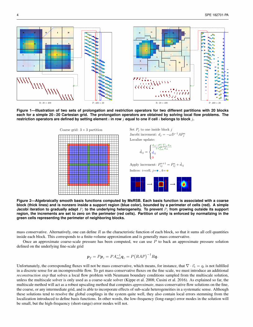
Most multiscale methods for Eq. 6 described in the literature start by introducing a non-overlapping coarse partition Ωjmj=1 ofthe fine grid, so that each cell Ωi in the fine grid belongs to a single block Ωj in the coarse grid. One then introduces a set ofbasis functions that map degrees of freedom associated with the coarse grid to degrees of freedom on the fine grid. To ensurethat this mapping is locally consistent with the properties of the differential operators in the flow equation, the basis functionsare computed numerically by solving localized flow problems. Although the basis functions can be set up to map both pressuresand velocities/fluxes, we will herein only consider finite-volume type methods solving for pressure as the primary variable. Inthis case, the basis functions can be collected into a numerical prolongation operator that maps pressure unknowns from thecoarse to the fine grid, P : Ωj → Ωi. We also define an analogous restriction operator that maps in the opposite directionR : Ωi → Ωj. These operators are represented as matrices P and R of size n × m and m × n, respectively. Figure 1illustrates pairs of (P,R) operators resulting from two different partitions of a rectangular grid.

By use of the prolongation operator, one can define an approximate fine-scale pressure pf = Ppc on Ω from any pressurepc defined on Ω. If we insert the approximate fine-scale pressure into Eq. 3, we get (AP )pc = q. This system contains moreequations than unknowns, and consequently we left-multiply by the restriction operator R to obtain a square linear system for theapproximate pressure,

(RAP )pc = Rq ←→ Amspc = qc. (7)

The physical interpretation of this coarse system depends on the choices made for P andR. Examples of P include the multiscalefinite-volume (MsFV) operator (Jenny et al. 2003), the multiscale two-point (MsTPFA) operator (Møyner and Lie 2014), or themultiscale restriction-smoothed-basis (MsRSB) operator (Møyner and Lie 2016b), which can all be obtained by fully algebraicconstructions. Figure 2 shows details of how prolongation operators are computed with the MsRSB method. For the restrictionoperator, one choice is to set R = PT , which corresponds to a Galerkin coarse-scale discretization, which unfortunately is not

4 SPE 182701-PA

P: 400× 20R: 20× 400 P: 400× 20R: 20× 400

Figure 1—Illustration of two sets of prolongation and restriction operators for two different partitions with 20 blockseach for a simple 20×20 Cartesian grid. The prolongation operators are obtained by solving local flow problems. Therestriction operators are defined by setting element i in row j equal to one if cell i belongs to block j.

Coarse grid: 3× 3 partition Set Pj to one inside block j

Jacobi increment: dj = −ωD−1APnj

Localize update:

dij =

dij−Pnij

∑k dik

1+∑

k dik

dij

0

Apply increment: Pn+1ij = Pn

ij + dij

Indices: i=cell, j= , k=

Figure 2—Algebraically smooth basis functions computed by MsRSB. Each basis function is associated with a coarseblock (thick lines) and is nonzero inside a support region (blue color), bounded by a perimeter of cells (red). A simpleJacobi iteration to gradually adapt Pj to the underlying heterogeneity. To prevent Pj from growing outside its supportregion, the increments are set to zero on the perimeter (red cells). Partition of unity is enforced by normalizing in thegreen cells representing the perimeter of neighboring blocks.

mass conservative. Alternatively, one can define R as the characteristic function of each block, so that it sums all cell quantitiesinside each block. This corresponds to a finite-volume approximation and is generally mass conservative.

Once an approximate coarse-scale pressure has been computed, we can use P to back an approximate pressure solutiondefined on the underlying fine-scale grid

pf = Ppc = PA−1msqc = P

(RAP

)−1Rq.

Unfortunately, the corresponding fluxes will not be mass conservative, which means, for instance, that∇ · ~vt = qt is not fulfilledin a discrete sense for an incompressible flow. To get mass-conservative fluxes on the fine scale, we must introduce an additionalreconstruction step that solves a local flow problem with Neumann boundary conditions sampled from the multiscale solution,unless the multiscale solver is only used as a coarse-scale solver (Kippe et al. 2008; Cusini et al. 2016). As explained so far, themultiscale method will act as a robust upscaling method that computes approximate, mass-conservative flow solutions on the fine,the coarse, or any intermediate grid, and is able to incorporate effects of sub-scale heterogeneities in a systematic sense. Althoughthese solutions tend to resolve the global couplings in the system quite well, they also contain local errors stemming from thelocalization introduced to define basis functions. In other words, the low-frequency (long-range) error modes in the solution willbe small, but the high-frequency (short-range) error modes will not.

SPE 182701-PA 5

To get a solver that is able to compute the fine-scale solution of Eq. 6 to within a prescribed residual distance – that is, alsoreduce the high-frequency error components – we need to cast the multiscale method in an iterative framework. One possibilityis to define a Richardson iteration

pk+1 = pk + ωkA−1ms(q −Apk). (8)

It is also possible to use A−1ms as a preconditioner for GMRES. Herein, we primarily consider two-stage algebraic multiscale

solvers (Wang et al. 2014), in which Ams is employed as a global preconditioner in combination with a local smoother W (A, b),i.e., any kind of inexpensive iterative solver that efficiently removes high frequency errors from the solution. Examples of possiblesmoothers include incomplete LU-factorization with zero or low degree of fill-in or standard iterative solvers including variantsof Gauss-Seidel or Jacobi’s method. With this in mind, we can define a two-step preconditioner that first removes local error byuse of the smoother and then computes a coarse scale correction,

xk+1/2 = xk +W (A, q −Axk), (9)

xk+1 = xk+1/2 + PA−1msR(q −Axk+1/2). (10)

The method above can easily be extended to more complex physics including both black-oil and compositional methods (Møynerand Lie 2016a; Hajibeygi and Tchelepi 2014; Møyner and Tchelepi 2017), and is essentially what is implemented as a prototypesolver in a commercial environment (Lie et al. 2017b; Kozlova et al. 2016).

The two-stage multiscale preconditioner will typically have a satisfactory initial convergence rate, which eventually dete-riorates when the remaining modes of the error are neither captured by the multiscale operator nor the local smoother. Theseintermediate modes can often be neglected and for many cases it is sufficient to reconstruct a conservative velocity field after amoderate number of iterations. Mathematically, two-stage multiscale solver is equivalent to the typical two-stage methods usedin the construction of algebraic multigrid solvers (Vanek et al. 1996). Philosophically, the multiscale method is different fromclassical multigrid methods, which use hierarchical grids constructed to accurately resolve all error modes by use of a multistagesolver and converge to a strict tolerance.

For cases with complex geology it may not be sufficient to only use the multiscale operator along with a local stage toaccurately capture the flow in an efficient manner. The convergence may stagnate before the desired tolerances are reached anda large number of iterations may be required to resolve the fluid displacements in the subsequent transport problem. In the nextsection, we will therefore extend the multiscale framework with additional basis functions to ensure favorable problem-specificconvergence rates, without increasing the size of the coarse systems that are the bottleneck for scaling to parallel systems. By useof operators from different coarse grids, one can hope to reduce the number of intermediate modes for cases when these are notnegligible.

Multiscale solver with multiple basis setsWe introduce the notion of multiple basis functions, so that we have N different prolongation operators P 1, . . . , PN , where eachP ` contains an individual set of basis functions corresponding to a distinct coarse grid Ω`

jm`j=1. Likewise, we will also associate

a set of restriction operators, R1, . . . , RN . To fit to the framework, the individual operators P ` and R` must fulfill the followingthree requirements:

1. The prolongation operator P ` for pressure and the restriction operator R` are constructed over non-overlapping partitionsof the fine grid. Each column j in P ` is referred to as a basis function and is associated with a coarse grid block Ω`

j .

2. The support of each basis function is compact and must contain the associated coarse block. Hence, for the support regionS`j of the jth basis function, we have Ω`

j ⊂ S`j ⊂ ∪m`j=1Ω`

j .

3. The columns of P ` form a partition of unity over the fine grid; that is, each row in P ` has unit row sum.

The N multiscale operators can all have different choices of coarse grids and support regions, and can also come from differenttypes of multiscale methods. For each multiscale operator, the initial coarse blocks, support regions, and basis functions areassumed to be created at the start of the simulation or in a preprocessing (offline) stage. Examples of multiscale methods that fitthis description include the MsFV (Jenny et al. 2003), MsTPFA (Møyner and Lie 2014), and MsRSB Møyner and Lie (2016b)methods. Of these, the MsRSB method is most robust and by far the simplest to implement for complex grids and coarsepartitions. This will therefore be our method of choice in the subsequent numerical experiments. Notice that the memory costof introducing additional multiscale operators is modest. Since each basis function only has support within a localized supportregion, the basis functions can be stored compactly with a memory requirement limited upward by the number of fine-scale cellstimes the maximum number of support regions overlapping a single cell. For a rectangular partition of a 2D Cartesian grid withn cells, for instance, this would amount to n integers to represent the partition and approximately 4n integers and 4n doubles torepresent the support regions and nonzero elements of the associated basis functions. Feature-specific operators tend to have verylimited overlap in support regions and hence give very modest increase in memory consumption.

6 SPE 182701-PA

If we let B` = P `(R`AP `)−1R` denote the multiscale solution operator corresponding to the `-th set of basis functions andlet W ` denote the corresponding local stage solver (smoother), then successive application of the different multiscale and localstages can be written as the multiplicative multistep method,

xk+`∗ = xk+`−1 +W `(A,dk+`−1) (11)

xk+` = xk+`∗ +B` dk+`∗, (12)

where the defect is defined as d = q−Ax and k is an integer multiple of N . Here, we have let the iteration count increase by Nif the multistage algorithm cycles through N different multiscale operators to simplify subsequent comparisons with the standarditerative MsFV and MsRSB methods. The presentation can be made more transparent if we consider the homogeneous case withq = 0 and assume that the application of each smoother corresponds to a multiplication with a matrix W `. Then the multistepmethod reads,

xk+N = BNWNxk+N−1 =[BNWN

][BN−1WN−1

]xk+N−2 = · · · =

[BNWN

]· · ·[B1W 1

]xk

=[PN (RNAPN )−1RN

]WN · · ·

[P 1(R1AP 1)−1R1

]W 1xk.

(13)

The multiscale preconditioners can also be combined in other ways, e.g., in an additive manner or in sequence without theapplication of a smoother between each multiscale operator. In the following, we will always include at least one set of generalbasis functions that cover the domain relatively evenly and constitute a reasonably accurate multiscale solver on their own. Inaddition, we will include specific basis functions that, through coarsening strategies or a specialized basis construction, aim tocapture specific features of the problem not captured by the general basis functions. The benefit of this is that key features inthe reservoir model affecting reservoir pressure – such as faults, fractures, wells that gets turned on or exhibit large changes inwell controls – can all be addressed by distinct fit-for-purpose multiscale operators in a very flexible manner. If necessary, thebasis functions and the shape and extent of coarse grid blocks and support regions can also be updated between the applicationof each multiscale preconditioner B` to reflect changes in driving forces and in reservoir and fluid properties. The fact that eachprolongation operator forms a partition of unity makes it very easy to enable or disable individual multiscale preconditionersduring the course of a simulation run. This would be hard to achieve if all the different and specialized basis functions werelumped together in a single multiscale operator that would need to be recalibrated to ensure partition of unity whenever a particularbasis function is added or removed.

The coarse partitions can be formed in many different ways. Partition methods include, but are not restricted to:

• Partitions formed by rectilinear or structured subdivision in physical space or in index space.

• (Un)structured mesh partitions generated by graph partitioning algorithms like in Metis (Karypis and Kumar 1998) thatoptionally can use transmissibilities or other measures of connection strength to ensure that each coarse block has ashomogeneous rock properties as possible, see e.g., (Møyner and Lie 2016b).

• Partitions adapting to geological features such as facies, rock types, saturation regions, geological layers, faults, etc, or toother meta-information coming from the geological modeling tool, see e.g., (Hauge et al. 2012; Hauge 2010).

• Partitions arising from block-structured griding, local grid refinement (LGR), or local coarsening.

• Partitions resulting from agglomeration of grid cells based on indicator functions set by the user, derived from the geologicalmodel, or from a preexisting simulation to give flow-adapted coarse grids, see e.g., (Hauge et al. 2012; Hauge 2010; Lieet al. 2017a)

• Partitions based on error measures/indicators, adjoint sensitivities, etc.

• Partitions adapting dynamically to evolving flow fields, saturations and compositions.

A few examples of such partitions are shown in Figure 3. For brevity, the different partitioning methods will not be discussedfurther. However, we will discuss how to improve the approximation of wells in some more detail.

Well basis functions By default, the global viscous forcing from wells are only accounted for on the coarse grid in a multiscalemethod, which may introduce quite inaccurate approximations, especially in the important near-well region on the fine-scale grid.This can be mitigated either by refining the coarse grid near the wells (Møyner and Lie 2016b), or by use of correction functionsthat are constructed analogously to the basis functions themselves, with source terms included (Wolfsteiner et al. 2006; Skaflestadand Krogstad 2008; Jenny and Lunati 2009). Both these approaches are somewhat limiting in that the choice of coarse grid forthe basis functions significantly influences the quality of the pressure approximation near the source terms.

To treat well terms and other singularities in a more independent manner, we introduce a set of well basis functions, with acorresponding coarse grid determined a posteriori from the near-well pressure profile. For a problem with nw different wells,

SPE 182701-PA 7

(a) Structured partition from’cookie-cutter’

(b) Graph partition withtransmissibility weights

(c) Specific partition adaptedto high-permeable channels

(d) Blocks agglomerated withtime-of-flight indicator

(e) Blocks agglomerated withpermeability indicator

(f) Blocks agglomerated withvelocity indicator

Figure 3—Illustration of various types of coarse partitions for an unstructured Voronoi grid with sealing faults and high-permeable channels.

we define a local support region for each well W` consisting of all cells within a prescribed distance from the well. The distancecan either be the edge distance in a discrete cell graph, physical distance between well and cell centroids, or a more sophisticatedmeasure such as time-of-flight, if available. We proceed to solve local problems in each subdomain with zero boundary conditionsand each well control set to unitary bottom-hole-pressure. This gives a set of discrete pressure responses p` for each well `, whichare defined such that p`i is zero for cells Ωi outside the support region and nonzero for cells inside. The pressure response, limitedto the support region, is then rescaled so that the maximum pressure is equal to unity. To assemble a prolongation operator fromthese local solutions, we apply a scaling factor such that

∑nw

`=1 p`i ≤ 1 for all cells Ωi if different wells are in close proximity of

each other. We also add another basis function that has global support throughout the whole reservoir. We can then define thewell basis

Pw =

[Pw1 , P

w2 , ..., P

wnw, 1−

nw∑

`=1

Pw`

]. (14)

Since each individual solution is limited to [0, 1] and their sum is always less than or equal unity, we have a partition-of-unitywith nw + 1 basis functions. To define a coarse grid for this prolongation operator, we use the same trick as in (Møyner and Lie2016b) and assign each fine cell to the coarse block whose basis function has the largest value in this cell.

Efficient flux reconstruction The flux-reconstruction step of a finite-volume multiscale solver relies on the physical interpreta-tion of the coarse scale system Ams when constructed with the control-volume restriction operator,

(R)ji =

1, if Ωi ⊂ Ωj ,

0, otherwise.

The resulting coarse system corresponds to a coarse-scale finite-volume discretization with fluxes induced by the prolongatedpressure field. If we consider the continuous form, this can be stated as

∫

∂Ωj

~v · ~n dA =

∫

Ωj

q dV, ~v = −K∇p ∀ j ∈ 1, ...,m, . (15)

8 SPE 182701-PA

Equivalently, the coarse-scale equation for Ωj resulting from the application of the finite-volume restriction operator equals thesum of the conservation equations in Eq. 5 for each fine cell Ωi in Ωj ,

∑

Ωi⊂Ωj

∑

f ⊂ ∂Ωi

Tf[(pms)N2(f) − (pms)N1(f)

]= (16)

∑

f ⊂ ∂Ωj

Tf[(pms)N2(f) − (pms)N1(f)

]=

∑

Ωi⊂Ωj

qi ∀ j ∈ 1, ...,m. (17)

Because all fluxes between cells inside the same coarse block cancel, the coarse-scale equations give a conservative finite-volumescheme. Hence, the conservative fluxes on Ω can be used as boundary conditions to compute conservative fine-scale fluxes insideeach coarse block. Following Lunati and Lee (2009), we define the matrix for the reconstruction problem from the fine-scalelinear system as

(D)kl =

(A)kl, if Ωk and Ωl belong to the same coarse block,0, otherwise,

(18)

The problem for the reconstructed pressure p is then a linear system with boundary conditions estimated from the multiscalepressure,

Dp = q − (A−D)pms = q. (19)

This linear system is in reality a collection of independent, local subproblems. In practice, however, these local problems maystill take up a large fraction of the overall simulation time as they must be inverted at the end of each pressure solve if onesubsequently wants to solve a transport problem at the fine scale.

By use of multiple sets of basis functions, it is possible to significantly reduce the cost of reconstructing the fluxes. Assumethat our method has two multiscale operators with coarse grids Ω1 and Ω2, restriction operators R1 and R2, and prolongationoperators P 1 and P 2. After the second multiscale operator has been applied, pms gives conservative fluxes across the interfacesof Ω2, but not across the interfaces of Ω1 (unless the interfaces of these two coarse partitions coincide). To construct mass-conservative fine-scale fluxes, we need to solve a series of local flow problems, one for each block Ω2

j , defined as

Dj pj = qj . (20)

However, instead of solving these independent problems directly, we first apply the multiscale operator corresponding to Ω1

inside Ω2j ,

p1 = P 1(R1DjP1)−1R1(qj − Dj pms) + pms.

where P 1 signifies the restriction of P 1 to Ω2j . By the same argument as in Eq. 17, this updated pressure p1 results in mass-

conservative fluxes over the (coarse) interfaces of Ω1 inside Ω2j . Consequently, after this multiscale approximation, we have

obtained mass-conservative fluxes with subscale variation on all interfaces of the intersection of Ω1 and Ω2, which results inmuch smaller subdomains as seen in Figure 4. For each of these new subdomains, the local matrix is defined analogously to theoriginal reconstruction problem,

(G)kl =

(D)kl, if Ωk and Ωl belong to the same coarse block pair Ω1,Ω2,

0, otherwise,(21)

which has additional boundary conditions applied from the intermediate multiscale approximation, resulting in the final linearsystem,

Gp = q = q − (D −G)p1 = q − (A−D)pms − (D −G)p1. (22)

The process described in Eq. 20 to Eq. 22 can be repeated to account for more than two multiscale operators if needed. Thefine-scale flux field is recovered by computing fluxes on ∂Ω2 from pms, fluxes on ∂Ω1 from p1, and the remaining fine-scalefluxes from p. The interested reader should consult Kunze et al. (2013) for a discussion of the special case when the two coarsepartitions are nested.

For fully unstructured grids, the intersection of several different grids may result in blocks that are not contiguous. When thisoccurs, we merge the cells having the lowest value for the corresponding basis functions into the largest neighbor. Figure 4(c)shows a case taken from one of the numerical examples discussed in the next section. Here, the intersection of two unstructuredpartitions result in a block being subdivided into two disconnected components, outlined in black. In this case, the single isolatedblock will merge with the neighboring large blue block.

SPE 182701-PA 9

(a) Primal basis functions associated withthe blocks shown as black lines

(b) Dual basis localized to a specificcoarse block

(c) Disconnected subgrid

Figure 4—Illustration of how the reconstruction can be subdivided into smaller problems. The left plot shows how the firstset of basis functions associated with the primal blocks drawn as black lines is used to find fluxes that are coarse-scaleconservative over the primal grid, whereas the middle plot shows how the second set of basis functions associated withdual blocks drawn as red lines are used locally within each block to further reduce the reconstruction to the intersectionof the primal and dual blocks. The right plot shows a case with two intersection partitions, one shown by color and oneby red lines. The cells marked in gray are part of block 2 in the first partition, but after the intersection they form a newsubdomain consisting of two disconnected parts. Here, the single isolated cell is merged into the neighboring block 1shown in light blue color.

Numerical examples

In the following, we will report a series of experiments set up to illustrate that the framework is flexible with respect to varioustypes of coarse partitions and to examine the accuracy of the resulting multiscale solvers and how efficient they reduce the fine-scale residual toward machine precision. In all experiments, we use prolongation operators constructed by the MsRSB method(Møyner and Lie 2016b) and finite-volume restriction operators. These have been implemented by use of the open-source MatlabReservoir Simulation Toolbox (MRST), see (Lie et al. 2012; Lie 2016), and our implementation is a generalization of the methodincorporated into a commercial simulator environment (Lie et al. 2017b; Kozlova et al. 2016). Although our solvers are capable ofrunning problems with industry-standard flow physics, including both black-oil and compositional models, we will for simplicityonly present cases with incompressible single-phase flow or two-phase flow without capillary forces.

Layers of SPE 10 Horizontal layers of Model 2 from the 10th SPE Comparative Solution Project (Christie and Blunt 2001)seem to have become a de facto benchmark that is seen in virtually any paper on multiscale methods. The overall SPE 10 modelis described by a 60×220×85 Cartesian grid with cells of uniform size 20×10×2 ft3 with heterogeneity sampled from a Brentsequence, as seen in the North Sea. The upper 35 layers are from a shallow-marine Tarbert formation, which has a relativelysmooth heterogeneity with permeabilities following a lognormal distribution. The fluvial Upper Ness formation found in thebottom 50 layers consists of an intertwined pattern of long and high-permeable sand channels interbedded with low-permeablesandstone. To test the accuracy of our multiscale framework, we pick the bottom layer of the Tarbert formation, which is lesssmooth than most of the upper layers, as well as the bottom layer of the Upper Ness formation. The flow physics is two-phaseflow with linear relative permeabilities and equal viscosities. The domain is initially filled with a nonwetting fluid and a wettingfluid is injected along the north side of the model, driven by a unit pressure drop from the north to the south side.

For the Tarbert layer, we introduce two different rectangular partitions which are set up like the primal and dual partitionstypically used in the original MsFV method. The primal grid has 6 × 11 blocks, with smaller block sizes at the perimeter,whereas the dual grid has 5 × 10 blocks of uniform size. The upper-left plot in Figure 5 shows the two partitions plotted ontop of the permeability field. The next four plots in the upper row show the initial fine-scale pressure and approximate pressurescomputed by the multiscale method with primal partition, dual partition, and alternating partitions. We observe that the dualgrid gives a systematic error as a result of not using smaller blocks near the inflow and outflow boundaries. The primal partitionand the alternating combination of the two partitions gives approximate solutions that are visually similar and have comparablediscrepancies in the L2 norm, see Table 1, Not surprisingly, we observe a somewhat lower pointwise discrepancy when thecombined set of basis function from the primal and dual grid are used, as each spans different parts of the fine-scale pressurespace. For the Upper Ness layer, we use the 6 × 11 coarse grid to construct the first prolongation operator. For the secondprolongation operator, we first use the permeability to segment the domain into two regions representing the high-permeable sandchannels and the low-permeable mudstone, and then use Metis to partition each region separately. This gives an unstructuredgrid with irregular coarse blocks adapting to strong contrasts in the permeability. Although this may seem to be a good idea, the

10 SPE 182701-PA

log10(K) + partitions Reference Partition 1 (red) Partition 2 (black) Alternating Sw at 0.5 PVI

Figure 5—Multiscale pressure solutions computed for 35th and 85th layers of the SPE 10 model. For the Tarbert formationin the upper row, we use two rectangular partitions, a 6×11 and a 5×10 dual. For the Upper Ness formation in the lowerrow, we use the same 6×11 in combination with a partition that adapts to the permeability. Reference solutions forpressure and saturation are computed by use of a standard fine-scale finite-volume method.

Table 1—Discrepancies in L2 and L∞ norm compared with a fine-scale solution for multiscale solutions computed on the35th (Tarbert) and 85th (Upper Ness) layers of the SPE 10 model.

Tarbert Upper NessCoarse grid L2 L∞ L2 L∞Partition 1 0.0155 0.1174 0.0307 0.1782Partition 2 0.1710 0.3865 0.0791 0.5506Alternating 0.0198 0.0620 0.0293 0.2929

resulting multiscale approximation is significantly less accurate than with the regular partition in both the L2 and the pointwisenorm. With the exception of MsTPFA, all multiscale finite-volume methods reported in the literature lead to multipoint stencils onthe coarse grid. It is well known that one generally cannot guarantee monotone solutions for multipoint stencils (Nordbotten et al.2007). This deficiency is particularly evident for the MsFV method and can be attributed to inadequate localization assumptions(Wang et al. 2016). Nonmonotone solutions are more rare for MsRSB, but in this particular example, we see a tendency ofnonmonotonicity near the south-east corner. Combining the two partitions reduces the L2 error slightly and gives a somewhathigher pointwise discrepancy compare with the regular partition. Also in this case, we observe a tendency of nonmonotonicity.However, neither of the solutions have cell values outside the interval of the unit pressure drop.

Next, we introduce iterations with a single pass of ILU(0) as local smoother to improve the discrepancies reported in Table 1.In the iterative formulation, the method with combined partitions can be seen as a standard iterative multiscale method that appliesdifferent partitions in every second step in an alternating manner. Since different partitions generally will represent different errormodes, the convergence of the fine-scale residual reported in Figure 6 is vastly superior when alternating partitions are used bothfor the smooth Tarbert formation and the channelized Upper Ness formation.

A small fine-scale residual does not necessarily mean that the approximate solution will be able to propagate saturations andcomponents accurately. To also measure the transport properties of the multiscale approximation, we solve the pressure equationonce and then simulate the injection of 1 pore volumes of the wetting fluid with a fixed flux field. Figure 7 reports discrepanciesin saturations as a function of time compared with using the true fine-scale fluxes. For comparison, we also report discrepancies

SPE 182701-PA 11

0 20 40 60 80 100 120 140 160 180

Iterations

10-8

10-7

10-6

10-5

10-4

10-3

Resid

ual

Primal

Dual

Combined

(a) Tarbert, Layer 35

0 20 40 60 80 100 120 140 160 180 200

Iterations

10-8

10-7

10-6

10-5

10-4

10-3

10-2

Resid

ual

Primal

Metis

Combined

(b) Upper Ness, Layer 85

Figure 6—Convergence of the multiscale methods as an iterative solver for two horizontal layers of the SPE 10 model.

0 20 40 60 80 100

0

0.02

0.04

0.06

0.08

0.1

0.12

0.14

0.16

0.18

0.2

Primal

Dual

Combined

(a) Tarbert, Layer 350 20 40 60 80 100

0

0.05

0.1

0.15

0.2

0.25

Primal

Metis

Combined

(b) Upper Ness, Layer 85

Figure 7—Discrepancies in saturation for a fixed field computed by various multiscale solvers as function of time step.The solid lines is with one multiscale solve and the dashed lines with four multiscale/ILU(0) iterations.

for approximate flow fields computed with four multiscale iterations. Here, we see that we get flux fields with significantly moreaccurate transport properties when two different coarse partitions are used. Note that we have employed the less inexpensive,local reconstruction for the combined solver.

Well basis To assess the accuracy of well basis functions, we consider two different permeability realizations on a 100 × 100rectangular grid, see Figure 8. The first is a Gaussian permeability field with a mean of 125 md, whereas the second case consistsof four layers with log-normal distributions in each layer and mean values varying from 50 to 500 md. A modified five-spot wellpattern is used to drive flow, consisting of an injector in the middle of the domain and four producers in the corners. All wellsare vertical and perforated in a single cell, except for the horizontal producer near the southwest corner, which is perforated in15 cells. Instead of a fixed injection rate, which is common in papers discussing multiscale methods, we set wells to operate ata fixed bottom-hole pressure. The amount of injected fluids will then depend on the quality of the pressure approximation. Theinjector operates at a fixed pressure of 500 bar, whereas the producers operate at 75, 100, 110 and 125 bar, respectively.

We consider three different multiscale solvers. The first is the original MsRSB method with a 6 × 6 coarse grid, in whichthe wells are located approximately at the block centroids. This is the ideal situation for a rectangular grid with source termsthat are defined on an underlying fine grid. The second uses well basis functions entirely on their own, thereby giving a verycoarse multiscale solver. The third solver combines well basis functions with the regular MsRSB partition. For the first part ofthis example, we have set the well distance to a radius of 15 cells, which, given the underlying structured fine-grid, results in

12 SPE 182701-PA

(a) Gaussian permeability (b) Layered permeability

Figure 8—The two 100×100 test problems used to illustrate well basis functions.

Table 2—Discrepancies in L2 and L∞ norm compared with a fine-scale solution for the two different permeability distri-butions used to illustrate use of well basis functions.

Gaussian LayeredBasis L2 L∞ L2 L∞MsRSB 0.0641 0.1679 0.0619 0.1750Well basis (d=15) 0.0760 0.1131 0.1015 0.1215Well basis + MsRSB 0.0303 0.1136 0.0280 0.0634

circular support regions for the well basis functions. Table 2 reports the discrepancies from the fine-scale solution for the threesolvers. We observe that the well basis or a regular partition on their own give larger discrepancies than when the two are usedin combination. If we examine the pressure fields in Figure 9, it is clear that basis functions defined in a regular partition willaverage out the impact of each well over the coarse blocks, giving inadequate detail near the wells. The well basis captures thenear-well pressure responses accurately, but because these functions are only supported near the wells, their predictive qualityis poor in the middle of the reservoir. The combined solver resolves both the global features and the local flow field accurately.The main purpose of using the well basis functions is to improve the approximation error in the near-well regions. Outside theseregions, the basis functions are constant and will hence not contribute significantly to improve convergence when used as iterativepreconditioners, which is confirmed in Figure 10.

To investigate how well the three approximate solvers resolve the transport properties of the fine-scale flow field, we solvea passive tracer flow problem in the fixed velocity fields given by each solver over a period normalized to the time it takes toinject one pore volume in the fine-scale, exact solver. Figure 11 reports the corresponding discrepancies in tracer concentration.We observe that the error is larger for the pure multiscale solver than for the well basis, which in turn is outperformed by thecombined solver. Computing the flux field is very expensive for the case with only well basis compared to the other two cases,since the subdomains used for reconstruction for the five basis functions are large and consequently expensive to invert.

Finally, we perform a systematic test to investigate how the initial error behaves as a function of the distance d used todetermine the radius of the near-well zone. The distance is systematically varied between d = 0 (no well basis, only MsRSB)and d = 50 (well bases cover the entire domain, and bases for the different wells overlap). Results reported in Figure 12 showthat there is a relatively rapid decay in errors initially for both permeabilities, which eventually decays as the near-well effects arecompletely captured at d ≈ 20.

Unstructured grid with faults and high-permeable channels For this example, we consider an unstructured Voronoi grid in2D with 8560 fine cells adapting to faults, high-permeable channels, and wells Klemetsdal et al. (2017). The model seen inFigure 13 contains 5 intersecting faults and 13 high-permeable channels. The faults have a transmissibility multiplier of 0.01 andare thus blocking flow from passing through, but the faults are also intersected by the network high-permeable channels. Thehigh-permeable channels have 5000 md permeability, which is a large contrast to the Gaussian background matrix permeabilitydistribution having a mean of 100 mD. To get an accurate fine-scale solution, the grid has smaller cells near the faults, wellsand faults. Flow is driven by an injector-producer pair controlled at 500 and 200 bar bottom-hole pressures. The flow pattern iscomplex, with large jumps in pressure over the faults and high-permeable channels dominating the saturation distribution (see

SPE 182701-PA 13

Fine-scale reference Regular partition Well basis Combined

Figure 9—Pressure solutions for the two permeability distributions with different solvers; the upper row is the log-normalcase and the bottom row the layered case.

0 20 40 60 80 100 120 140 160 180 200

Iterations

10-8

10-7

10-6

10-5

10-4

10-3

10-2

10-1

100

Resid

ual

Coarse

Wells

Wells+Dual

(a) Gaussian permeability

0 20 40 60 80 100 120 140 160 180 200

Iterations

10-8

10-7

10-6

10-5

10-4

10-3

10-2

10-1

100

Resid

ual

Coarse

Wells

Wells+Dual

(b) Layered permeability

Figure 10—Convergence of the multiscale methods with well basis functions as iterative solvers for the two different testcases from Figure 8.

14 SPE 182701-PA

0 20 40 60 80 100

% PVI

0

0.02

0.04

0.06

0.08

0.1

0.12

0.14

0.16

0.18

0.2

Err

or

Coarse

Wells

Wells+Dual

(a) Gaussian permeability

0 20 40 60 80 100

% PVI

0

0.02

0.04

0.06

0.08

0.1

0.12

0.14

0.16

0.18

0.2

Err

or

Coarse

Wells

Wells+Dual

(b) Layered permeability

Figure 11—Concentration error for the well basis example for two different permeability realizations.

0 10 20 30 40 50

Well basis radius

0

0.02

0.04

0.06

0.08

0.1

0.12

0.14

0.16

0.18

0.2

Pre

ssure

err

or

L2

L∞

(a) Gaussian permeability

0 10 20 30 40 50

Well basis radius

0

0.02

0.04

0.06

0.08

0.1

0.12

0.14

0.16

0.18

0.2

Pre

ssure

err

or

L2

L∞

(b) Layered permeability

Figure 12—Discrepancy between the fine-scale solution and the multiscale pressure approximation as a function of well-basis size.

Figure 14) and constitutes a challenging test for multiscale solvers.The example is intended to illustrate the situation where a model contains a large number of features that affect the flow

pattern, and we will investigate to what extent we can improve the accuracy of the multiscale solution by use of partitions thatadapt to these features. The baseline multiscale solver relies on a rectangular partition in physical space, consisting of 10 × 10coarse blocks that do not account for any spatial features. In addition, we consider a Metis partition with the same numberof coarse blocks, for which the graph partitioning strikes a balance between automatically adapting to the geological featuresas represented in the system matrix and creating coarse blocks that minimize communication volume and discrepancy in blocksizes. To get adapt coarse grids to high-permeable channels and faults, we perform an additional Metis partitioning in whichconnections over faults and between the high-permeable channels and the background sand have been removed. To focus on thelocal features, we allow up to 500% variation in block sizes and use half the number of degrees-of-freedom compared with theother coarse grids. Finally, we include the well basis functions described in the previous example.

Table 3 reports the initial discrepancy between the multiscale approximation and the fine-scale solution. We observe thatthe MsRSB method generally gives accurate results regardless of the partition used, but that the Metis grid clearly outperformsthe structured coarse grid, which does not take connection strengths of the system into account. Combining different partitions,the best results are obtained when rectangular or Metis partitions are used together with well basis functions. Considering thesaturation discrepancies for a linear displacement problem in Figure 15, we observe that there seems to be a steady improvementin accuracy as additional features are added to the approximation. The feature-adapted basis functions, however, do not seem togive any improvement compared to the same solver with only generic basis functions. In the convergence plot for the Richardsoniterations, however, we see that including the basis functions for the local features significantly improves the convergence rate.

SPE 182701-PA 15

(a) 2D Voronoi grid with faults (redlines), high-permeable channels (bluelines), and wells (red circles)

(b) Permeability field: colors show log10(K) withhigh-permeable channels drawn as red lines

(c) Coarse partitions: red lines = rectan-gular, green lines = Metis partition, bluelines = object/fault partition

Figure 13—Setup for the test case with an unstructured grid that adapts to faults, high-permeable channels, and wells.

(a) Fine-scale pressure (b) Saturation front at 0.5 PVI

Figure 14—Reference solution for the unstructured test case.

Table 3—Discrepancies between the fine-scale pressure solution and multiscale approximations computed with differentcombinations of coarse partitions for the 2D unstructured grid example with and without well basis functions.

Multiscale With well basisSolver L2 L∞ L2 L∞(1) Cartesian(100 dof) 0.0110 0.05232 0.0197 0.0345(2) Metis (100 dof) 0.0192 0.06431 0.0106 0.0270(3) Channels separated (50 dof) 0.0215 0.07867 0.0157 0.0471(1 + 2) 0.0123 0.03351 0.0080 0.0192(1 + 2 + 3) 0.0119 0.03359 0.0077 0.0145

16 SPE 182701-PA

0 10 20 30 40 50 60 70 80 90 100

0

0.05

0.1

0.15

0.2

0.25

0.3

Global basis

Global + well basis

Cart

Metis

Features

Cart + Metis

All three

(a) Saturation discrepancy as function of time step. Dashed lines cor-respond to solution with well basis functions included.

0 10 20 30 40 50 60 70 80 90 100

0

0.005

0.01

0.015

0.02

0.025

0.03

(b) Saturation discrepancy after 12 iterations as function of time step.Dashed lines correspond to solution with well basis functions included.

0 20 40 60 80 10010

-12

10-10

10-8

10-6

10-4

10-2

100

Hexahedral

METIS

Frac

Combined+well

Combined+well+frac

Combined

(c) Convergence rates

Figure 15—Saturation discrepancies and convergence rates for the unstructured test case.

Gullfaks Our last example revisits a test case from (Møyner and Lie 2016b). The simulation model of the Gullfaks fieldfrom the Norwegian sector of the North Sea is a challenging example of a real geological model with strong petrophysicalheterogeneity, large anisotropy and aspect ratios, degenerate cell geometries, and unstructured grid topology. The geology consistsof several reservoir zones, including delta sandstones, shallow-marine sand, fluvial-channel and delta-plain formations, with themain production coming from Brent sands (i.e., from the same sedimentary environment seen in the SPE 10 model). The structuralmodel has rotated fault blocks in the west and a structural horst in the east, with a highly faulted area in between. The simulationmodel therefore has a large number of sloping faults, with angles varying from 30 to 80 degrees and throws from zero to 300 m;see (Fossen and Hesthammer 1998) for more details. Out of the 416 000 cells in the 80×100×52 corner-point grid, 216 344 cellsare active and 44% of these have non-neighboring connections. When interpreted as a matching grid, cells will have betweenfour and thirty-one faces. In our experience, it is almost impossible to generate consistent primal–dual partitions necessary tocompute MsFV basis functions. On the other hand, the grid has a rich structure that can be utilized to define adapted partitionsand MsRSB-type basis functions.

We consider two different partitioning strategies: (i) a rectangular partition in logical space in which we split blocks acrossintersecting faults, and (ii) a Metis partition with the same number of grid blocks computed with graph weights derived from thefine-scale transmissibilities. We construct two coarse grids of each type: The first rectangular grid is built from logical blocksconsisting of 12×12×15 fine cells, giving a total of 447 coarse blocks after splitting across faults. The high degree of coarseningin the vertical direction is somewhat misleading, as the model contains a large number of inactive layers and eroded cells. Thesecond grid uses a coarsening factor 5 × 5 × 8 and has 2530 blocks. Likewise, we construct two Metis partitions with 447 and2530 blocks. Figure 16 shows excerpts of the two coarse grids with 447 blocks.

SPE 182701-PA 17

(a) Fine grid colored by log10(Kx) (b) Subset of rectangular blocks (c) Subset of Metis blocks

Figure 16—The Gullfaks simulation model partitioned into 447 blocks.

Table 4—The discrepancy between the fine-scale solution and approximate multiscale solutions with different partitionsfor the Gullfaks test case.

Multiscale With well basisSolver L2 L∞ L2 L∞(1) Cartesian (447 blocks) 0.0365 0.2299 0.0261 0.2785(2) Metis (447 blocks) 0.0331 0.1527 0.0190 0.0800(3) Cartesian (2530 blocks) 0.0344 0.3325 0.0155 0.2895(4) Metis (2530 blocks) 0.0153 0.1699 0.0143 0.1605(1 + 2) 0.0270 0.1966 0.0124 0.2863(3 + 4) 0.0159 0.6544 0.0053 0.2888

To drive flow through the model, we set up a simple well pattern consisting of two vertical injectors and three verticalproducers. The discrepancies in the initial multiscale solutions reported in Table 4 are somewhat inconclusive: using only theMetis partition gives the lowest pointwise discrepancy, whereas combining both partitions and well basis functions gives thelowest L2 error. On the other hand, the discrepancies are very low, given the low number of coarse blocks and the complexity ofthe geological model. This testifies both to the robustness and the accuracy of the MsRSB method. Moreover, the convergenceplots reported in Figure 18 confirm once again that employing (at least) two different partitions will generally reduce more errormodes and give significantly faster convergence when the multiscale method is used as an iterative solver.

A word of caution at the end: the Metis partitions and the intersection of the Metis partitions and the rectangular partitionswill give blocks with irregular geometry and in some cases high inter-block variation in petrophysical properties. If all the localsystems are collected into one global matrix, this matrix will have very poor condition number and local rescaling of the individualsubsystems is required if one wants to use a direct solver to invert all the systems in one operation.

SummaryIn this paper we have introduced a flexible framework for combining multiple multiscale operators to solve the flow equations inporous media. In a series of test cases we demonstrate how this framework can be used to combine one or more generic multiscaleoperator defined to have good resolution for the entire reservoir with specific multiscale operators tailored to particular featuresof the reservoir model, such as well patterns, high-permeable channels, or regions with different rock types. The new frameworkis easy to implement, provides better approximate solutions and faster convergence rates at a very modest cost. In particular, theframework is applicable to real reservoir models with challenging high contrast geology, complex reservoir geometry with a largenumber of faults, and complex unstructured grids.

AcknowledgmentsThis research was funded in part by Schlumberger Information Solutions and by the Research Council of Norway under grantno. 226035.

ReferencesAkkutlu, I. Y., Efendiev, Y., Vasilyeva, M., and Wang, Y. 2017. Multiscale model reduction for shale gas transport in a coupled discrete fracture

and dual-continuum porous media. J. Nat. Gas Sci. Eng. doi: 10.1016/j.jngse.2017.02.040.

Bush, L., Ginting, V., and Presho, M. 2014. Application of a conservative, generalized multiscale finite element method to flow models. J.Comput. Appl. Math., 260:395–409. doi: 10.1016/j.cam.2013.10.006.

18 SPE 182701-PA

(a) Fine-scale (b) Cart (c) Metis

(d) Cart + Metis (e) Wells + Cart + Metis

Figure 17—Pressure solutions computed for the Gullfaks model partitioned with 447 blocks.

0 20 40 60 80 100

Iterations

10-8

10-6

10-4

10-2

100

Resid

ual

Cart: 447

Metis: 447

Cart: 2530

Metis: 2530

Cart+Metis: 447

Cart+Metis: 2530

Figure 18—Convergence of the multiscale solver with various partitions for the Gullfaks test case. Dashed lines corre-spond to solvers with the well basis functions included as a separate stage.

SPE 182701-PA 19

Christie, M. A. and Blunt, M. J. 2001. Tenth SPE comparative solution project: A comparison of upscaling techniques. SPE ReservoirEval. Eng., 4:308–317. doi: 10.2118/72469-PA.

Chung, E. T., Efendiev, Y., and Li, G. 2014. An adaptive GMsFEM for high-contrast flow problems. J. Comput. Phys., 273:54–76. doi:10.1016/j.jcp.2014.05.007.

Cortinovis, D. and Jenny, P. 2014. Iterative Galerkin-enriched multiscale finite-volume method. J. Comput. Phys., 277:248–267. doi:10.1016/j.jcp.2014.08.019.

Cortinovis, D. and Jenny, P. 2017. Zonal multiscale finite-volume framework. J. Comput. Phys., 337:84–97. doi: 10.1016/j.jcp.2017.01.052.

Cusini, M., van Kruijsdijk, C., and Hajibeygi, H. 2016. Algebraic dynamic multilevel (ADM) method for fully implicit simulations of multi-phase flow in porous media. Journal of Computational Physics, 314:60–79. doi: 10.1016/j.jcp.2016.03.007.

Dolean, V., Jolivet, P., Nataf, F., Spillane, N., and Xiang, H. 2014. Two-level domain decomposition methods for highly heterogeneous Darcyequations. Connections with multiscale methods. Oil & Gas Science and Technology – Rev. IFP Energies nouvelles, 69(4):731–752. doi:10.2516/ogst/2013206.

Efendiev, Y., Galvis, J., and Hou, T. Y. 2013. Generalized multiscale finite element methods (GMsFEM). J. Comput. Phys., 251:116–135. doi:10.1016/j.jcp.2013.04.045.

Efendiev, Y., Galvis, J., and Wu, X.-H. 2011. Multiscale finite element methods for high-contrast problems using local spectral basis functions.J. Comput. Phys., 230(4):937–955. doi: 10.1016/j.jcp.2010.09.026.

Efendiev, Y. and Hou, T. Y. 2009. Multiscale Finite Element Methods, volume 4 of Surveys and Tutorials in the Applied Mathematical Sciences.Springer Verlag, New York.

Fossen, H. and Hesthammer, J. 1998. Structural geology of the Gullfaks Field. In Coward, M. P., Johnson, H., and Daltaban, T. S., editors,Structural geology in reservoir characterization, volume 127, pages 231–261. Geological Society Special Publication.

Hajibeygi, H. and Tchelepi, H. A. 2014. Compositional multiscale finite-volume formulation. SPE J., 19(2):316–326. doi: 10.2118/163664-PA.

Hauge, V. L. 2010. Multiscale Methods and Flow-based Gridding for Flow and Transport in Porous Media. PhD thesis, Norwegian Universityof Science and Technology.

Hauge, V. L., Lie, K.-A., and Natvig, J. R. 2012. Flow-based coarsening for multiscale simulation of transport in porous media. Comput.Geosci., 16(2):391–408. doi: 10.1007/s10596-011-9230-x.

Hou, T. Y. and Wu, X.-H. 1997. A multiscale finite element method for elliptic problems in composite materials and porous media. J. Comput.Phys., 134:169–189. doi: 10.1006/jcph.1997.5682.

Jenny, P., Lee, S. H., and Tchelepi, H. A. 2003. Multi-scale finite-volume method for elliptic problems in subsurface flow simulation. J. Comput.Phys., 187:47–67. doi: 10.1016/S0021-9991(03)00075-5.

Jenny, P. and Lunati, I. 2009. Modeling complex wells with the multi-scale finite-volume method. J. Comput. Phys., 228(3):687 – 702. doi:10.1016/j.jcp.2008.09.026.

Karypis, G. and Kumar, V. 1998. A fast and high quality multilevel scheme for partitioning irregular graphs. SIAM J. Sci. Comp., 20(1):359–392.doi: 10.1137/S1064827595287997.

Kippe, V., Aarnes, J. E., and Lie, K.-A. 2008. A comparison of multiscale methods for elliptic problems in porous media flow. Comput. Geosci.,12(3):377–398. doi: 10.1007/s10596-007-9074-6.

Klemetsdal, Ø. S., Berge, R. L., Lie, K.-A., Nilsen, H. M., and Møyner, O. 2017. Unstructured gridding and consistent discretizationsfor reservoirs with faults and complex wells. In SPE Reservoir Simulation Conference, 20-22 February, Montgomery, Texas, USA. doi:10.2118/182666-MS.

Kozlova, A., Walsh, D., Chittireddy, S., Li, Z., Natvig, J., Watanabe, S., and Bratvedt, K. 2016. A hybrid approach to parallel multiscalereservoir simulator. In ECMOR XV – 15th European Conference on the Mathematics of Oil Recovery, Amsterdam, The Netherlands. EAGE.doi: 10.3997/2214-4609.201601889.

Kunze, R., Lunati, I., and Lee, S. H. 2013. A multilevel multiscale finite-volume method. J. Comput. Phys., 255:502–520. doi:10.1016/j.jcp.2013.08.042.

Lie, K., Krogstad, S., Ligaarden, I. S., Natvig, J. R., and Nilsen, Halvor an d Skaflestad, B. 2012. Open-source MATLAB implementation ofconsistent discretisations on complex grids. Comput. Geosci., 16:297–322. doi: 10.1007/s10596-011-9244-4.

Lie, K.-A. 2016. An Introduction to Reservoir Simulation Using MATLAB: User guide for the Matlab Reservoir Simulation Toolbox (MRST).SINTEF ICT, http://www.sintef.no/Projectweb/MRST/publications, 3rd edition.

20 SPE 182701-PA

Lie, K.-A., Kedia, K., Skaflestad, B., Wang, X., Yang, Y., and Wu, X.-H. 2017a. A general non-uniform coarsening and upscaling frameworkfor reduced-order modelling. In SPE Reservoir Simulation Conference, Montgomery, TX, USA, 20–22 February 2017. SPE 182681-MS, doi:10.2118/182681-MS.

Lie, K.-A., Møyner, O., Natvig, J. R., Kozlova, A., Bratvedt, K., Watanabe, S., and Li, Z. 2017b. Successful application of multiscale methodsin a real reservoir simulator environment. Comput. Geosci. doi: 10.1007/s10596-017-9627-2.

Lie, K.-A., Natvig, J. R., Krogstad, S., Yang, Y., and Wu, X.-H. 2014. Grid adaptation for the Dirichlet–Neumann representation method andthe multiscale mixed finite-element method. Comput. Geosci., 18(3):357–372. doi: 10.1007/s10596-013-9397-4.

Lunati, I. and Lee, S. H. 2009. An operator formulation of the multiscale finite-volume method with correction function. Multiscale Model.Simul., 8(1):96–109. doi: 10.1137/080742117.

Manea, A., Hajibeygi, H., Vassilevski, P., and Tchelepi, H. A. 2016. Enriched algebraic multiscale linear solver. In ECMOR XV–15th EuropeanConference on the Mathematics of Oil Recovery. doi: 10.3997/2214-4609.201601894.

Manea, A., Hajibeygi, H., Vassilevski, P., and Tchelepi, H. A. 2017. Parallel enriched algebraic multiscale solver. In SPE Reservoir SimulationConference, , 20-22 February, Montgomery, Texas, USA. doi: 10.2118/182694-MS.

Møyner, O. and Lie, K.-A. 2014. A multiscale two-point flux-approximation method. J. Comput. Phys., 275:273–293. doi:10.1016/j.jcp.2014.07.003.

Møyner, O. and Lie, K.-A. 2016a. A multiscale restriction-smoothed basis method for compressible black-oil models. SPE J., 21(6):2079–2096.doi: 10.2118/173265-PA.

Møyner, O. and Lie, K.-A. 2016b. A multiscale restriction-smoothed basis method for high contrast porous media represented on unstructuredgrids. J. Comput. Phys., 304:46–71. doi: 10.1016/j.jcp.2015.10.010.

Møyner, O. and Tchelepi, H. A. 2017. A multiscale restriction-smoothed basis method for compositional models. In SPE Reservoir SimulationConference, Montgomery, TX, USA, 20–22 February 2017. SPE 182679-MS, doi: 10.2118/182679-MS.

Nordbotten, J., Aavatsmark, I., and Eigestad, G. 2007. Monotonicity of control volume methods. Numer. Math., 106(2):255–288. doi:10.1007/s00211-006-0060-z.

Skaflestad, B. and Krogstad, S. 2008. Multiscale/mimetic pressure solvers with near-well grid adaption. In Proceedings of ECMOR XI–11thEuropean Conference on the Mathematics of Oil Recovery, number A36, Bergen, Norway. EAGE. doi: 10.3997/2214-4609.20146387.

Vanek, P., Mandel, J., and Brezina, M. 1996. Algebraic multigrid by smoothed aggregation for second and fourth order elliptic problems.Computing, 56(3):179–196. doi: 10.1007/BF02238511.

Wang, Y., Hajibeygi, H., and Tchelepi, H. A. 2014. Algebraic multiscale solver for flow in heterogeneous porous media. J. Comput. Phys.,259:284–303. doi: 10.1016/j.jcp.2013.11.024.

Wang, Y., Hajibeygi, H., and Tchelepi, H. A. 2016. Monotone multiscale finite volume method. Comput. Geosci., 20(3):509–524. doi:10.1007/s10596-015-9506-7.

Wolfsteiner, C., Lee, S. H., and Tchelepi, H. A. 2006. Well modeling in the multiscale finite volume method for subsurface flow simulation.Multiscale Model. Simul., 5(3):900–917. doi: 10.1137/050640771.