spatiotemporal behavior and nonlinear dynamics in a … · spatiotemporal behavior and nonlinear...
TRANSCRIPT

NASA Contractor Report 4567
/ i /f
I
/
Spatiotemporal Behavior
and Nonlinear Dynamics in
a Phase Conjugate Resonator
Siuying Raymond Liu
GRANT NAG1-1363
DECEMBER 1993
https://ntrs.nasa.gov/search.jsp?R=19940019056 2018-07-17T05:59:33+00:00Z

i
NASA Contractor Report 4567
Spatiotemporal Behavior
and Nonlinear Dynamics in
a Phase Conjugate Resonator
Siuying Raymond Liu
Virginia Polytechnic Institute and State University
Blacksburg, Virginia
Prepared for
Langley Research Center
under Grant NAG1-1363
National Aeronautics andSpace Administration
Office of Management
Scientific and Technical
Information Program
1993
(NASA-CR-4567) SPATIOTEMPORAL
BEHAVIOR AND NONLINEAR 0YNAMICS
A PHASE CONJUGATE RESONATOR
(Virginia Polytechnic Inst. and
State univ.) 225 p
IN
H1/74
N94-23529
Unclas
0203383


Spatiotemporal behavior and nonlinear dynamics in a
phase conjugate resonator
by
Siuying Raymond Liu
Committee Chairman: Prof. Guy Indebetouw
Department of Physics
ABSTRACT
The work described in this dissertation can be divided into two parts. The first
part is an investigation of the transient behavior and stability property of a phase
conjugate resonator (PCR) below threshold. The second part is an experimental and
theoretical study of the PCR's spatiotemporal dynamics above threshold.
The time-dependent coupled wave equations for four-wave mixing (FWM) in a
photorefractive crystal, with two distinct interaction regions caused by feedback from
an ordinary mirror, was used to model the transient dynamics of a PCR below thresh-
old. Analytical expressions of the steady state cavity's fields for the case of nonde-
pleted pumps and an absorption free medium were derived and used to determine the
self-oscillation conditions. The solutions, through simple frequency domain transfor-
mation techniques, were used to define the PCR's transfer function and analyse its
stability.
Taking into account pump depletion and medium absorption, the transient buildup
and decay times of the cavity's fields as well as the specularly reflected and phase
conjugate reflected intensities were numerically calculated as functions of a number
of system parameters such as the coupling parameter and the pump and probe ratios.
General trends were unveiled and discussed in view of the possible use of the PCR in
image storage or processing architectures. Experimental results for the buildup and
decay times confirmed qualitatively the predicted behavior.
Experiments were carried out above threshold to study the spatiotemporal dynam-
ics of the PCR as a function of the Bragg detuning achieved by misaligning one of the
two pump beams and of the degree of transverse confinement controlled by varying
P_G PAGE BLANK NOT FN._Oiii

the resonator'sFresnelnumber. The temporal aspectsof the beam'scomplexity were
studied by local intensity time series,powerspectra,and reconstructedpseudophase
portraits. An irregular time serieswasidentified asdeterministic chaoshaving a cor-
relation dimensionof 5.2and a Kolmogoroventropy of 0.16s-1. Experimental results
varying both control parametersrevealedthe presenceof two distinct frequenciesin
the power spectra in someregionsof the parameterspace. The existenceof optical
vortices in the wavefrontwereidentified by interferometry. The spatial complexity of
the beam was studied in terms of the spatial distributions of optical vortices, their
trajectories and their relationship to the beam'sspatial coherence.
The transversedynamicsand the spatiotemporal instabilities were also described
by modeling the three dimensionalcoupledwaveequationsin photorefractiveFWM,
using a truncated modal expansionapproach. Numerical solutionsof the model re-
vealed the presenceand motion of optical vortices in the wavefront. Simulations
using the Bragg detuning asa control parametershowedthat optical vorticesappear
as long asa largeenoughmodulation of the wavefrontis brought about by local gain
enhancementresulting from the small misalignmentof one of the pump beamsfrom
the Bragg angle. Powerspectra of simulated time seriesalso contain two distinct
frequenciesfor a certain rangeof the off-Bragg parameter. Maps of the spatial cor-
relation index werefound to be templatesof the correspondingmapsof the vortices'
trajectories, indicating that the dynamicsmay be defect-mediated.
iv

A CKN OWLED G EMENT S
While working on this research and writing of this thesis, I have benefited greatly
from the kind assistance, gentle encouragement and helpful suggestions of many peo-
ple. Here are those whom I would like to thank especially:
Prof. Guy J. Indebetouw, my mentor and thesis supervisor, who shaped my
intellectual life, shared patiently and cheerfully his knowledge of physics with me
during many interesting discussions, introduced me to the field of photorefractive
wave mixing and optical oscillators, suggested the problem which eventually led to
this work and provided me with financial support during much of my stay at Virginia
Tech. This thesis would not have been possible without his help.
Prof. Silverio P. Almeida, my advisor, who introduced me to optics during my
early years at Virginia Tech..
Prof. Clayton D. Williams, my thesis committee, who provided resourcefully the
care and support needed in pursuit of my research and career.
Prof. Dale D. Long, my thesis committee, who shared with me his many ideas
and excitements of teaching physics; encouraged and helped me to be aware of and
familiar with areas related to educational physics.
Prof. Randy J. Heflin, my thesis committee, who shared his knowledge of nonlinear
optics and provided me insightful and articulate discussion and comments.
Prof. Ira Jacobs, my thesis committee, who served in my committee as a spe-
cialist in his field of nonlinear fiber optics and sacrified research time to review this
manuscript.
V

Prof. R. L. Bowden, my teacher, who never forgot to remind me that there is
more fun in teaching than just research.
Dr. Peter Lo and Dr. Caisy Ho, my officemates and colleagues during my early
years in the Optical Coherent Lab, who made the Lab a special place to work.
Calvin Doss and Dan Korwan, my fellow colleagues, who made the basement floor
a fun and lively forum.
Reinaldo Gonzalez and Xijun Zhao, my colleagues and friends, who shared over
the years the laughters and their feelings about everything from physics to politics
and to life.
Dave Miller and Bob Ross, from the Machine Shop, who made the accessories for
my experiments.
Dale Schutt, Roger Link and Grayson Wright, from the Electronic Shop, who
supplemented electronic instruments and made gadgets for my experiments; assisted
me with the computing facilities in the Physics department.
Dr. Sharon Welch and Dave Cox, from the Spacecraft Control Branch of NASA/Langley,
who provided invaluable help and timely support of accessing the computing machines
there.
Anonymous referees for their helpful and insightful comments on articles that are
made up of most parts of this thesis.
The National Aeronautics and Space Administration at Langley for supporting
me with a 2-year research fellowship.
vi

TABLE OF CONTENTS
Introduction 1
1.1 Background ................................ 1
Dissertation outline ............................ 4
The photorefractive effect, wave mixing and real time holograhy . . . 6
2 The PCR model: steady state analysis 12
2.1 Introduction ................................ 12
2.2 Model of the PCR below threshold ................... 13
2.2.1 The Cavity ............................ 13
2.2.2 The Four-wave mixing (FWM) equations ............ 17
2.2.3 The material's constants ..................... 19
2.3 Steady-state analysis ........................... 24
2.3.1 Steady-state equations and their solutions ........... 25
2.3.2 Threshold for self-oscillation ................... 27
2.4 Transfer function of the PCR and its stability analysis ........ 29
2.4.1 Frequency domain transformation of the PCR's equations... 29
2.4.2 Transient response and its stability ............... 32
2.5 Conclusion ................................. 36
vii

3 Transient behavior of a PCR: numerical study 37
3.1 A numerical approach .......................... 38
3.1.1 The start of the transients ................... 38
3.1.2 Adiabatic elimination algorithm ................. 39
3.2 Numerical analysis ............................ 41
3.2.1 Response curves for the cavity fields .............. 41
3.2.2 Cavity response time ....................... 48
3.2.3 Specular and conjugate reflections ................ 54
3.3 Experimental results ........................... 54
3.3.1 Experimental setup ........................ 58
3.3.2 Measurement of the cavity response time ............ 58
3.4 Conclusion ................................. 66
Temporal and spatial instabilities 67
4.0.1 Nonlinear systems ......................... 68
4.1 Characterization of chaotic dynamics .................. 70
4.1.1 Fourier spectra .......................... 70
4.1.2 Phase space portraits and attractors .............. 74
4.2 Dimensions ................................ 75
4.2.1 Kolmogorov entropy ....................... 79
4.2.2 Dimensions and phase space portraits from an experimental
time series ............................. 80
4.3 Background on spatiotemporal chaos .................. 81
4.3.1 Extended systems. Weak turbulence .............. 81
4.3.2 Topological turbulence ...................... 84
°°.
VIll

4.3.3 Methodologies of spatiotemporal complexity .......... 85
4.4 Wavefront dislocations/phase defects .................. 88
5 Experiments: spatiotemporal dynamics in PCRs 96
5.1 Experimental setup ............................ 97
5.2 Time series, Power spectra and Phase space portraits ......... 101
5.3 Correlation dimension and Kolmogorov entropy ............ 108
5.4 Wavefront dislocations .......................... 114
5.5 Defect-mediated turbulence ....................... 123
5.6 Modes superposition ........................... 130
5.7 Discussions and conclusions ....................... 135
6 A model of spatiotemporal dynamics in PCRs
6.1
6.2
6.3
139
Introduction ................................ 139
The modal expansion model ....................... 140
6.2.1 Phase-conjugate resonator .................... 140
6.2.2 Modal decomposition ....................... 144
Numerical results ............................. 148
6.3.1 Local intensity fluctuations .................... 150
6.3.2 Vortices and spatial correlation ................. 155
Experimental results ........................... 164
Summary and conclusions ........................ 173
7 Conclusion 176
7.1 Discussions and summaries ........................ 176
7.2 Possible future investigations ....................... 181
ix

Appendix A Derivation of the four-wave mixing equations .............. 183
Appendix B The Kukhtarev's equations ........................................ 190
X
LIST OF FIGURES
1.1 Two-beam coupling and hologram formation in the photorefractive
crystal ...................................
1.2 Photorefractive four-wave mixing geometry ...............
2.1 Schematic diagram for a phase conjugate resonator with a two-path
geometry ..................................
2.2 Schematic diagram for a two-crystal cavity ...............
2.3 Geometrical configuration of two-wave mixing in a photorefractive ma-
terial ....................................
2.4 Steady state PCM reflectivity as a function of the pump ratio for var-
ious values of the coupling parameter ..................
2.5 Feedback parameter as a function of the pump ratio for various values
of the coupling parameter .........................
2.6 Plots of the transfer function for the PCR below threshold ......
2.7 Plots of the transfer function for the PCR near threshold .......
2.8 Plots of the transfer function for the PCR above threshold threshold .
3.1 Response curves of the cavity field intensity for various values of the
coupling parameter ............................
3.2 Response curves of the cavity field intensity for various values of the
pump ratio ................................
7
10
14
16
20
28
30
33
34
35
42
44
xi

3.3
3.4
3.5
3.6
3.7
3.8
3.9
3.10
3.11
3.12
3.13
3.14
3.15
3.16
3.17
Response curves of the cavity field intensity for various values of the
probe ratio .................................
Response curves of the cavity field intensity for various values of the
input mirror's reflectivity .........................
Response curves of the cavity field intensity for various values of the
medium's absorption parameter .....................
The cavity's buildup time as function of the pump ratio for various
values of the coupling parameter .....................
The cavity's decay time as function of the pump ratio for various values
of the coupling parameter ........................
The cavity's buildup time as function of the probe ratio for various
values of the pump ratio .........................
The cavity's decay time as function of the probe ratio for various values
of the pump ratio .............................
The response of the PCR to a short seed pulse .............
The response curves of the specular and conjugate reflections of the
PCR for low coupling parameter .....................
The response curves of the specular and conjugate reflections of the
PCR for high coupling parameter .....................
Diagram of the experimental setup for the PCR's transient dynamics
Typical cavity field response to a square pulse input from which the
buildup and decay times were measured .................
Experimental buildup time as a function of the pump ratio for two
values of the coupling parameter .....................
Experimental decay time as a function of the pump ratio for two values
of the coupling parameter .........................
Experimental buildup time as a function of the probe ratio ......
xii
45
46
47
49
51
52
53
55
56
57
59
6O
62
63
65
3.18 Experimental decaytime asa function of the probe ratio ....... 66
4.1
4.2
4.3
4.4
4.5
4.6
4.7
4.8
4.9
Schematicdiagram showingthe possibleoutputs from a linear system
and a nonlinearsystem ..........................
Lorenz'schaotic time series .......................
Lorenz's "butterfly" effect ........................
70
72
73
Illustration of the method of coveringa 1-and 2-dimensionalsetof points 77
Schematicdiagramof the Rayleigh-Benardconvection......... 84
Phasecontoursof a travelling wavecontaining a pure edgedislocation 91
Wavefrontsof a travelling wavecontaining a pure screwdislocation 93
Examplesof dislocations' motion in a travelling wave ......... 94
More examplesof dislocations' movementsin a travelling wave .... 95
5.1 Schematicdiagramof the experimentalsetup for the study of the spa-
tiotemporal dynamicsin PCR ...................... 99
5.2 Phaseconjugate intensity and the buildup times of the PCR above
thresholeagainst the pump raito for variousvaluesof the total pump
powers ................................... 101
5.3 Time seriesfor varying the Fresnelnumber in the PCR ........ 104
5.4 Powerspectra for varying the Fresnelnumber in the PCR ....... 105
5.5 Phasespaceportraits for varying the Fresnelnumber in the PCR 107
5.6 Time seriescontainsthe intermittent bursts for F -- 5.8 ........ 108
5.7 Log-log plots of orrelation intergral C2(e) versus distance e ...... 111
5.8 Local slope v(e) of the correlation integral versus log e ......... 112
5.9 Plot of the correlation dimension for each embedding dimension d 113
5.10 Value of the entropy K2,d versus the embedding dimension d ..... 114
°,o
Xlll

5.11 Sequence of snapshots of the irradiance distribution for F -- 2.2 . . . 116
5.12 Instantaneous interferogram for F = 2.2 ................ 117
5.13 Sequence of snapshots for F = 3.6 .................... 119
5.14 Instantaneous interferogram for F = 3.6 ................ 120
5.15 Sketches of some typical motions of the defects observed ....... 121
5.16 Sequence of snapshots for F = 4.1 .................... 122
5.17 Instantaneous interferogram for F = 4.1 ................ 123
5.18 Sequence of snapshots for F = 5.8 .................... 125
5.19 Instantaneous interferogram with F = 5.8, showing only one pair of
defects ................................... 126
5.20 Instantaneous interferogram with F = 6.8 ............... 127
5.21 Maximum number N of defects observed in the transverse pattern ver-
sus Fresnel number F ........................... 128
5.22 Spatial correlation index versus Fresnel number F ........... 130
5.23 Sequence of patterns motion obtained by the superposing three TEM
modes ................................... 133
5.24 Motions of two conjugate defects projected on a plane ......... 134
5.25 Computer-generated snapshots of an interferogram with a spherical
reference wave ............................... 135
5.26 Experimental snapshots of the interferograms of wavefront containing
a defect with a spherical reference wave ................. 137
6.1 Model on a four-wave mixing in a PCR ................. 142
6.2 Time series of local intensity /4 for different values of the off-Bragg
parameter ................................. 152
6.3 Bifurcation diagram of the local intensity /4 as a function of the off-
Bragg parameter ............................ 153
xiv
6.4 Power spectra of a local intensity /4 as a function of the off-Bragg
parameter ................................. 154
6.5 Phase space portraits of local intensity/4 as function of the off-Bragg
parameter ................................. 155
6.6 The profile of the absolute value of the field amplitude IAal showing
four holes in the beam cross-section ................... 157
6.7 Phase contour map identifies the four holes in the wavefront ..... 158
6.8 Time evolution of the modulus of the field amplitude A4 along a line
x = 1 for different values of the off-Bragg parameter .......... 159
6.9 Profile of the correlation index distribution ............... 162
6.10 Snapshots of sequence of interferograms reveal the motions of two pairs
of defects for the off-Bragg parameter bd = -2.45 ........... 163
6.11 Trajectories of defects and profile of correlation index for the off-Bragg
parameter bd = -2.45 .......................... 164
6.12 Defect trajectories and profile of correlation index for off-Bragg param-
eter bd = -2.55 .............................. 166
6.13 Trajectories of defects and profile of correlation index for the off-Bragg
parameter bd = -2.75 .......................... 167
6.14 Sequence of snapshots of interferograms for the off-Bragg parameter
bd = -3.18 ................................. 168
6.15 Profile of correlation index for off-Bragg parameter bd = -3.18 .... 169
6.16 Interferogram snapshot at the output of the PCM revealing the pres-
ence of two pairs of vortices of opposite charges ............ 171
6.17 Experimental time series of local intensity of/4 for different values of
the off-Bragg parameter ......................... 172
6.18 Power spectra of the experimental time series for different values of the
off-Bragg parameter ............................ 173
XV

6.19 Time delayed phase space portraits obtained from experimental time
series for different values of the off-Bragg parameter .......... 175
A.1 Four-wave mixing geometry ....................... 186
B.1 Hologram formation in a photorefractive material using four-wave mix-
ing scheme ................................. 193
xvi

Chapter 1
Introduction
1.1 Background
Optical feedback has been widely used in image processing since the late 1970s.
Its applications include image restoration and recovery, pattern recognition, and the
implementation of optical associative memory. Historically, optical feedback in ana-
log processors was first proposed to extend their range of optical operations and to
increase their performance and accuracy. Systems with passive coherent feedback
have been demonstrated in spatial filtering, computing the solutions of differential
equations, image restoration, and the implementation of nonlinear operation [1]. Yet,
the performance of these passive feedback systems is limited by the cavity losses and
by the accumulation of phase errors in each round trip.
Theorectical work on optical feedback suggested that fast analog optical devices
with feedback can implement slowly converging iterative algorithms [2, 3]. Itera-
tive algorithms are often needed in problems such as image restoration and recovery
as well as in recognition and associative recall. Efficient optical implementations of
these algorithms, however, require active feedback with a regenerative feedback loop
in which the signal energy and its phase after each iteration can be restored. In the
feedback loop, to amplify the light, two type of gain devices have been experimen-
CHAPTER 1. INTRODUCTION
tally demonstrated in all-optical systems: dye amplification [4, 5] and photorefractive
amplification [6, 7].
Amplified phase conjugation via four-wave mixing (FWM) with two antiparallel
pump beams in a photorefractive medium can not only compensate for the cavity
losses, but also cancel the aberrations and phase distortions acquired in each round
trip. One advantage of photorefractive nonlinearities over other nonlinear mechanisms
is that efficient beam interactions and large gain coefficients can now be achieved
with a few tens of milliwatts of laser power in materials such as bismuth silicon oxide
Bi12SiO2o. Low-power cw phase conjugate resonator (PCR) oscillations were recently
demonstrated using a barium titanate BaTiOa crystal as a phase conjugate mirror
(PCM) [81.
Since the successful demonstration of the photorefractive oscillators, a variety of
all-optical architectures was proposed for the realization of optical neural comput-
ers [9, 10, 11]. Most of the systems demonstrated so far are dealing with associative
recall in which a partial information input can address the holographically stored
images. The image having the highest correlation peak is selected and reconstructed.
The PCMs in the systems are used to provide optical feedback, thresholding and gain,
the three essential building blocks of a neural network system [12, 13, 14].
About a quarter of a century ago, an optical phenomenon now known as the
photoreffactive effect was discovered in lithium niobate LiNbOa and called at that
time the "optical damage". The undesirable optical damage in nonlinear and electro-
optical crystals turned out to be an advantage when using these materials as holo-
graphic optical memories. However, the interest in holographic memory in these
media quickly declined because the stored information was being erased during the
read-out process or lost subsequently after the pumps are turned off. For a while, as
the basic understanding of the origin of the effect and its potential use in eliminating
wavefront distortion became known, photorefractive wave mixing and phase conju-
gation has grown rapidly into a sub-discipline in the field of nonlinear optics. In the
middle 19708, the science of the photorefractive effect became mature. More knowl-
edge of the electro-optic media and their characteristic properties was available. The
CHAPTER 1. INTRODUCTION
previously unwanted degradation of optical memories was recognized as exactly what
is needed for real time holography. Up until a few years ago, most of the research
in that field was concerned with the steady-state behavior of wave mixing in pho-
torefractive media and its applications [15, 16]. Recently, however, there has been an
increasing interest in the dynamics of these processes. As more practical devices are
built exploiting photorefractive phase conjugation, we would like to know how these
systems respond to the temporal variations of any of their parameters. Knowledge
of the dynamical behaviors of such systems makes it possible to design devices and
predict their performance. Also of interest, even for steady-state applications, is the
stability of various wave-mixing schemes. For a device based on these principles, one
would like to predict if the system will be stable for the ranges of parameter values
over which the desired operations must be performed.
The dynamics of wave mixing in photorefractive media were first considered in
early theorectical works of the transient behavior of two-wave mixing (TWM) [17].
They showed, for example, how the system approaches the steady state when only
one of the input beams is present and the other is abruptly turned on. Later work
examined the stability of photorefractive FWM processes [18, 19]. In addition, many
groups have recently reported observations of temporal instabilities and chaos in
photorefractive devices such as self-pumped PCMs [20, 21, 22], ring phase conjuga-
tors [23, 24], mutually pumped phase conjugators [25, 26], and PCRs [27, 28]. Several
models have been put forward to explain the dynamics of optical phase conjugation
found in photorefractive crystals [29, 30, 31, 32] and devices [33, 34, 35]. Different
mechanisms have been suggested to explain the temporal photorefractive instabilities.
In the model of reference [22], for example, the chaotic behavior of a photorefractive
PCM in a FWM geometry is shown to be caused by the existence of multiple inter-
action regions in the crystal. Instabilities also arise in PCMs having only a single
grating and a single interaction region [31]. Here, the factor leading to the chaotic
behavior is the presence of an external electric field causing a shift in the optical fre-
quency of the phase conjugate wave (PCW). A more recent model [32] even predicts
a chaotic behavior in the standard FWM geometry with a single interaction region
CHAPTER 1. INTRODUCTION
and no external electric field if two gratings, transmission and reflection, of similar
strength take part in the process. In ref. [35], two coupled ring cavities provide a
competition between nonlinear gain and loss which results in nonsteady oscillating
beams. It is thought that the competition for energy between different cavities re-
sembles the competition for energy between different channels inside the self-pumped
PCM [21] when it becomes unstable.
Thus far, all these models are based on the well-known one dimensional coupled
wave theory [36]. Therefore, they are incapable of describing the dynamics in the
transverse plane observed in experiments such as those reported in refs. [27, 28].
Besides, effects such as strong light scattering (fanning) in the crystals, or various
spatial effects of diffractions in resonators, all of which are found in real situations,
result in non-uniform gain of the beam profiles. These kinds of considerations will
require an extension of the one dimensional framework to a two or three dimensional
framework in the coupled-wave theory. Indeed, the geometry of the self-pumped
PCM has been considered in a three dimensional theory [37]. Furthermore, finite
gaussian beams have recently been used to study the beam profile deformation in
photorefractive TWM and FWM in a two dimensional framework [38]. These studies
have been dealing with the steady-state aspect of the transverse beam profiles in
photorefractive media. Yet, the transverse dynamics of nonlinear optical system is
becoming an increasingly important topic of research [39].
1.2 Dissertation outline
In this thesis, the study of the nonlinear dynamics in a PCR has been divided into
two parts. In the first part, we will investigate the transieni behavior and stability
property of a PCR below threshold. In the second part, we will study experimentally
and theoretically the PCR's spatiotemporal dynamics above threshold.
In chapter 2, we will present the model and the steady state analysis of a PCR
below threshold based on time-dependent coupled wave equations for FWM in a
CHAPTER i. INTRODUCTION
photorefractive crystal with two distinct interaction regions caused by feedback from
a slightly tilted ordinary mirror. The steady state equations for the cavity's field,
taking into account nondepleted pumps and absorption free medium, will first be
solved. The analytic solutions are used to discuss the threshold conditions. We also
find the PCR's transfer function by applying simple frequency domain transformation
techniques to the steady state equations. The transfer function is used to analyse the
stability of the PCR.
In chapter 3, the study will be extended to the transient regime of the PCR. We
will first apply a numerical scheme for integrating the coupled wave equations using
an adiabatic elimination process. We calculate the cavity's buildup and decay times
as well as the specularly reflected and phase conjugate reflected intensities as func-
tions of a number of system parameters. Numerical results indicate that the cavity
buildup and decay times can be tailored by varying several of the system parameters
to assess the possible use of the PCR as an image processing element. Experimental
measurements are shown to qualitatively confirm the numerical simulations.
In chapter 4, we will give a brief introduction to some of the terminlogy and
methods of nonlinear and chaotic dynamics, which are applied to the analysis of
experimental time series data and to the beam's spatial complexity in the dynamics
of PCR above threshold.
In chapter 5, we will present experimental results for the dynamics of PCR above
threshold. We study by experiments some aspects of the spatiotemporal behaviors of
the PCR as a function of the resonator's Fresnel number by varying one of the two
apertures inside the cavity. Temporal aspects of the beam's complexity will be studied
analysing the local intensity time series, power spectra, and embedded phase space
portraits. A range of parameters is found for which the time series exhibit chaotic
variations. For the spatial aspects of the beam's complexity, we will give evidence for
the presence of wavefront dislocations or vortices in the optical field by using video
recording and interferometry. A rich variety of defect movements are recorded and
analysed. The spatial complexity is characterized by the number of optical vortices
and their variety of movements as well as their relationship with the beam's spatial

CHAPTER 1. INTRODUCTION
coherence.
In chapter 6, we will present and test a model based on a truncated modal expan-
sion of the cavity modes, to investigate the spatiotemporal dynamics of the PCR. We
find the optical vortices in the optical field's wavefront in the numerical solutions. Nu-
merical calculations are performed using the Bragg detuning, achieved by misaligning
one of two pump beams as a control parameter. Numerical results indicate that the
loss of temporal coherence and the onset of temporal chaos in the local intensity fluc-
tuations are correlated to the loss of spatial confinement of the vortices' trajectories
and the spatial coherence. The validity of the model is verified by comparison with
experimental data.
In chapter 7, a conclusion and a summary for this work are given. Some possible
future investigations are suggested.
1.3 The photorefractive effect, wave mixing and real time
holography
In the remainder of this chapter, we begin a brief introduction to the photorefrac-
tive effect, wave mixing and phase conjugation, and then go on to the transients of
the PCR and the steady state analysis in the next chapter.
The photorefractive effect is a phenomenon in which the local index of refraction
is changed by a spatially varying light intensity. The effect has been observed in
crystals such as lithium niobate LiNbO3, barium titanate BaTiO3 and strontium
barium niobate SBN as well as in cubic crystals of the sillenite family such as bismuth
silicon oxide BSO.
Suppose that we illuminate a photorefractive crystal with two coherent plane elec-
tromagnetic waves as in fig. 1.1a. The waves will interfere with each other and pro-
duce a spatially varying (sinusoidal) light intensity pattern inside the crystal. Charge
carriers are optically excited into the conduction band in the bright regions of the
6

CHAPTER 1. INTRODUCTION
beam 4crystal
14(X) II(X)
I(x)
p(x)J |
Esc(x) ::_,
(a) (b)
Figure 1.1: Pictorial illustration of the formation of a phase hologram in electro-
optic crystals via the photorefractive effect. (a) Two coherent electromagnetic plane
waves write a sinusodial grating inside the crystal, (b) Spatial variations of the light
intensity I(x), charge carrier distribution p(x), space-charge field E(x) and refractiveindex n(x). After Hall et al. [15]
7
CHAPTER 1. INTRODUCTION
interference pattern and move by drift (due to any internal and/or externally applied
electric fields) and diffusion into the dark regions, where they are trapped. Thus,
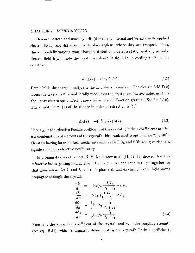
this sinusoidally varying space charge distribution creates a static, spatially periodic
electric field E(x) inside the crystal as shown in fig. 1.1b, according to Poisson's
equation:
V. E(z)= (1.1)
Here p(x) is the charge density, e is the dc dielectric constant. The electric field E(x)
alters the crystal lattice and locally modulates the crystal's refractive index n(x) via
the linear electro-optic effect, generating a phase diffraction grating. (See fig. 1.1b).
The amplitude An(x) of the change in index of refraction is [40]
An(x) = -(n3reH/2)E(x). (1.2)
Here r_i_ is the effective Pockels coefficient of the crystal. (Pockels coefficients are lin-
ear combinations of elements of the crystal's third rank electro-optic tensor 7_ijk [40].)
Crystals having large Pockels coefficients such as BaTiO3 and SBN can give rise to a
significant photorefractive nonlinearity.
In a seminal series of papers, N. V. Kukhtarev et al. [41, 42, 43] showed that this
refractive index grating interacts with the light waves and couples them together, so
that their intensities I, and/4 and their phases ¢1 and ¢4 change as the light waves
propagate through the crystal:
dI, _ I1 I4dz Re(%) I1 -t- 14
dI4 I, I4
dz - Re(%) 11 -q-14
1 14dz 2 Im(%) 11 -4- I4'
d¢4 1 I,
dz - _Im(%) I1 -4- 14"(1.3)
Here a is the absorption coefficient of the crystal, and 70 is the coupling strength
(see eq. B.54), which is primarily determined by the crystal's Pockels coefficients,
CHAPTER 1. INTRODUCTION
dielectric constant and interacting geometry. In the absence of any external fields
and if the charge migration in the crystal is dominated by diffusion, the resulting
index grating will be shifted by 90 ° with respect to the interference pattern, as shown
in fig. 1.1b, and the coupling strength "_o will be purely real.
It is the occurrence of the phase shift between the index grating and the interfer-
ence pattern that makes possible an asymmetric transfer of energy from one beam
to the other. This two-beam coupling phenomenon is known as two wave mixing.
According to equation 1.3, if the real part of the coupling strength, Re(_'o), is greater
than zero (it depends on the interaction geometry and the sign of the charge of the
charge carrier), the intensity/4 will grow with propagation while I1 will drop. Also,
for purely real 3'o, the phases of both beams remain unchanged as they travel through
the crystal.
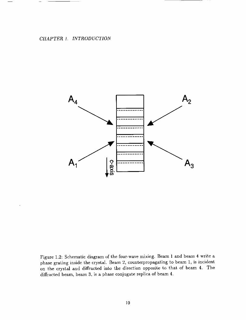
Suppose now that a third weak beam (beam 2) is incident to the crystal, in a
direction opposite to that of beam 1 as shown in fig. 1.2. This beam will be diffracted
by the phase grating into the direction opposite to that of beam 4. It can be shown
that this diffracted beam (beam 3) is the phase conjugate of beam 4. To see what
this means physically, let the beam 4 amplitude be written as
1 [A4(r)ei(_._._wt ) J- A,4(F)e_i(_.F_wt)] ' (1.4)E4( ,t) =
The phase conjugate wave (PCW) is obtained by taking the complex conjugate of
the spatial part of the wave in eq. 1.4:
1 [A,4(r)ei(_g._._,_t)+ A4(r)e_i(_g.e._,_t)], (1.5)Ep_(r,t) =
which can be rewritten as
Epc(r,t) = _[A*4(r)e -'(g'r+_t) + A4(r)ei(g'+'+_0], (1.6)
which is the time reversed version of the wave in eq. 1.4.
This generation of a time-reversal copy of the probe wave is called optical phase
conjugation. A photorefractive crystal employed to produce such a phase conjugate
CHAPTER 1. INTRODUCTION
A 4 A2
Figure 1.2: Schematic diagram of the four-wave mixing. Beam 1 and beam 4 write a
phase grating inside the crystal. Beam 2, counterpropagating to beam 1, is incident
on the crystal and diffracted into the direction opposite to that of beam 4. The
diffracted beam, beam 3, is a phase conjugate replica of beam 4.
10
CHAPTER 1. INTRODUCTION
wave back to its source is called a "phase conjugate mirror". The process we just
described involves four beams interacting and is referred to as "four-wave mixing".
H. Kogelnik, more than 25 years ago, demonstrated using conventional holography
that a distorted image could be undistorted by first producing its phase conjugate
replica and then sending it backward through the original distorter [44]. In conven-
tional holography, this involves a two-step procedure in which a photographic plate is
first used to store the interference pattern between the incoming distorted image and
a reference wave. This hologram is developed and repositioned exactly in its original
place. The hologram is then read out by a wave propagating in a direction opposite
to that of the original reference wave and deflects the reading wave to produce the
PCW.
Now, with the process of photorefractive FWM, the photorefractive crystal re-
places the photographic plate to store the hologram which is being written by an
image-bearing beam and a coherent reference beam. At the same time, the hologram
can be read out by a reading beam incident at the Bragg angle inside the crystal.
The simultaneous write and read processes eliminate the developing and fixing steps.
So the FWM gives us a new method of storing dynamic holograms in real time image
processing, which is often named "real-time holography".
11
Chapter 2
The P CR model: steady state
analysis
2.1 Introduction
Phase conjugate resonators (PCRs) are resonators in which at least one of the
mirrors is a phase conjugate mirror (PCM). The PCM, which acts both as a phase
conjugator and as a gain element, confers to the resonator some unique properties
(e.g. phase healing, transverse mode degeneracy, etc.) [45]. A number of applications
of the PCR to image processing have been demonstrated or proposed [7, 46, 9, 11].
A class of these applications makes use of the regenerative feedback of the PCR to
synthesize unusual transfer functions, perform nonlinear operations, or implement
iterative algorithms [7, 46]. Another type of problem which has motivated this study
more directly involves the implementation of discrete time algorithms for distributed
parameter control systems [47]. A PCR could be used as a real-time holographic
element for temporal image storage and delay operations. In all these, the PCR is
below threshold (for self-oscillation) and functions as a regenerative amplifier.
In these applications, the way in which the PCR responds to time-varying signals is
important for understanding the operation of the device. Therefore a theory is needed
12

CHAPTER 2. THE PCR MODEL: STEADY STATE ANALYSIS
to describe the transient effects in the PCR (such a theory is described in 2.2). Phase
conjugate Fabry-Perot cavities have recently been studied both in the steady state
case [48] and in the limit of a PCM with a fast response such as a Kerr material [49].
Fast response means that the time scale associated with the buildup of the polarization
field in the medium is much shorter than other time scales in the problem. Thus,
there is no difficulty in coupling the time dynamics of the material with the time
dynamics of the optical field in a self-consistent manner. However, this is not the
case in sluggish photorefractive materials such as in BaTi03 because the time scale of
the grating formation is not shorter than other time scales in the problem. Equations
for the transient behavior of the PCR with a sluggish medium must, therefore, include
the material equations.
In section 2.3, we first solve the steady state equations for the PCR, for the con-
ditions of nondepleted pumps and an absorption free medium. An analytic solution
can be obtained and used to describe the threshold conditions of the PCR. In the
quasi-steady state limit for a slow material, the steady state solution can also be used
to derive a transfer function for the PCR (section 2.4). The transfer function is then
used to analyse the transient response if there are some system operative ranges that
could lead to instability of the device.
2.2 Model of the PCR below threshold
In this section, we develop a model for a phase conjugate Fabry-Perot resonator
with a PCM consisting of a sluggish photorefractive material. The medium is modeled
by the standard Kukhtarev theory. Equations for the fields in the cavity and in the
medium, under the plane wave theory, are derived.
2.2.1 The Cavity
The geometry of the PCR is sketched in Figure 2.1. It consists of a conventional
(dielectric) mirror and an externally pumped PCM . The input beam AIN may make
13
CHAPTER 2. THE PCR MODEL: STEADY STATE ANALYSIS
M /1 t
rm, tm rm, tm
A41 _1
PCM
z=-L A1/ z=O z=d
/
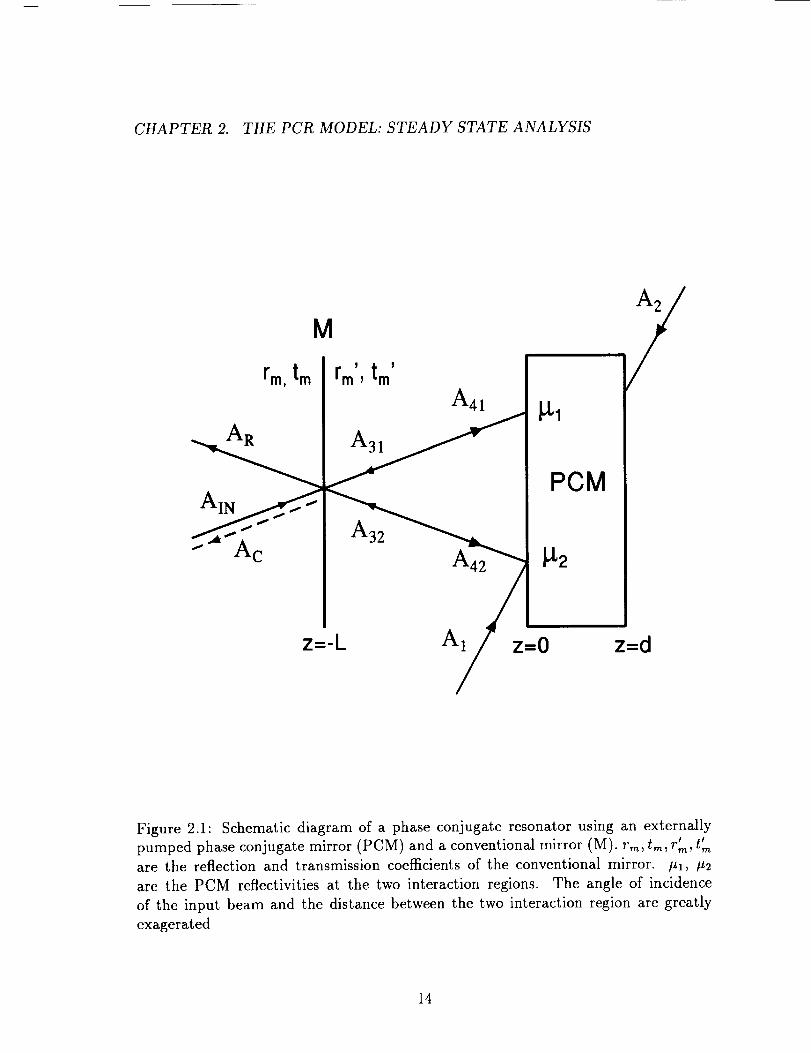
Figure 2.1: Schematic diagram of a phase conjugate resonator using an externally
pumped phase conjugate mirror (PCM) and a conventional mirror (M). rm, tin, rim, t"
are the reflection and transmission coefficients of the conventional mirror. #1, #2
are the PCM reflectivities at the two interaction regions. The angle of incidence
of the input beam and the distance between the two interaction region are greatly
exagerated
14
CHAPTER 2. THE PCR MODEL: STEADY STATE ANALYSIS
a small angle with the mirror normal so that in general two distinct interaction
regions exist in the PCM. The presence of two distinct gratings can easily be verified
experimentally.
A PCR formed by two PCMs has been investigated by others [50] and proposed
for the holographic storage of images [51]. The only difference between the cavity
of fig. 2.1 and the two-crystal cavity, as shown in figure 2.2, is that, in the two-
crystal set up, the pumps' intensities can be varied independently. In a single-crystal
cavity where the two interaction regions share the same pumps, the steady state PCM
reflectivities #1 and #2 are equal, although they generally grow at different rates.
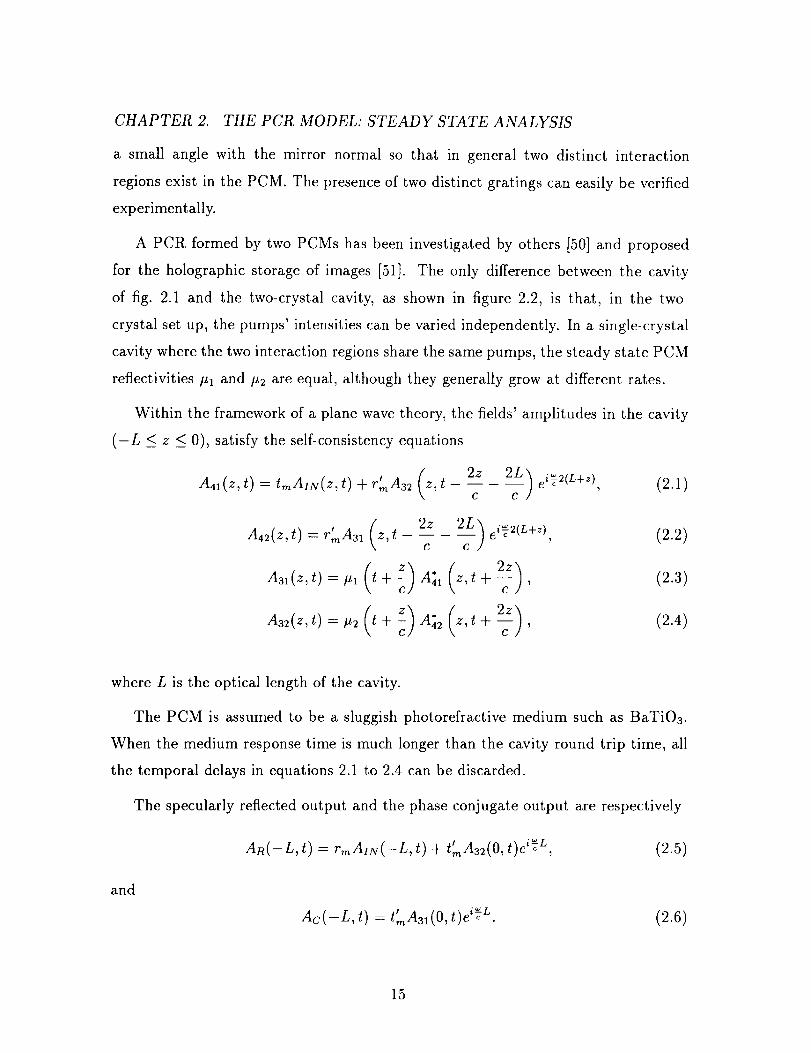
Within the framework of a plane wave theory, the fields' amplitudes in the cavity
(-L < z _< 0), satisfy the self-consistency equations
A41(z,t ) ----trnAIN(Z,_ ) -_ rtrnA32 (z,_ 2Zc 2L)c
= rmA31 z, tc c
A31(z,t) : #1 (_ _- z) A;1 (z,t-Ji- 2z) ,
(z)A3:(z,t) = ¢2 t+ A42 z,t + ,
ei_2(L+z), (2.1)
(2.2)
(2.3)
(2.4)
where L is the optical length of the cavity.
The PCM is assumed to be a sluggish photorefractive medium such as BaTiOa.
When the medium response time is much longer than the cavity round trip time, all
the temporal delays in equations 2.1 to 2.4 can be discarded.
The specularly reflected output and the phase conjugate output are respectively
AR(-L,t) = rmAiN(-L,t) + t_A32(O,t)e i_L, (2.5)
and
Ac(-L,t) = t_A31(O,t)e i_L. (2.6)
15

CHAPTER 2. THE PCR MODEL: STEADY STATE ANALYSIS
_1,1
PCM1
II
_,,A,,,,/
Beam Splitter
/_A21 AT
AIN
_2
PCM2
/_A22
A21
/
Figure 2.2: Two-crystal cavity comparable to the cavity with two interaction regions
of figure 2.1.
16
CHAPTER 2. THE PCR MODEL: STEADY STATE ANALYSIS
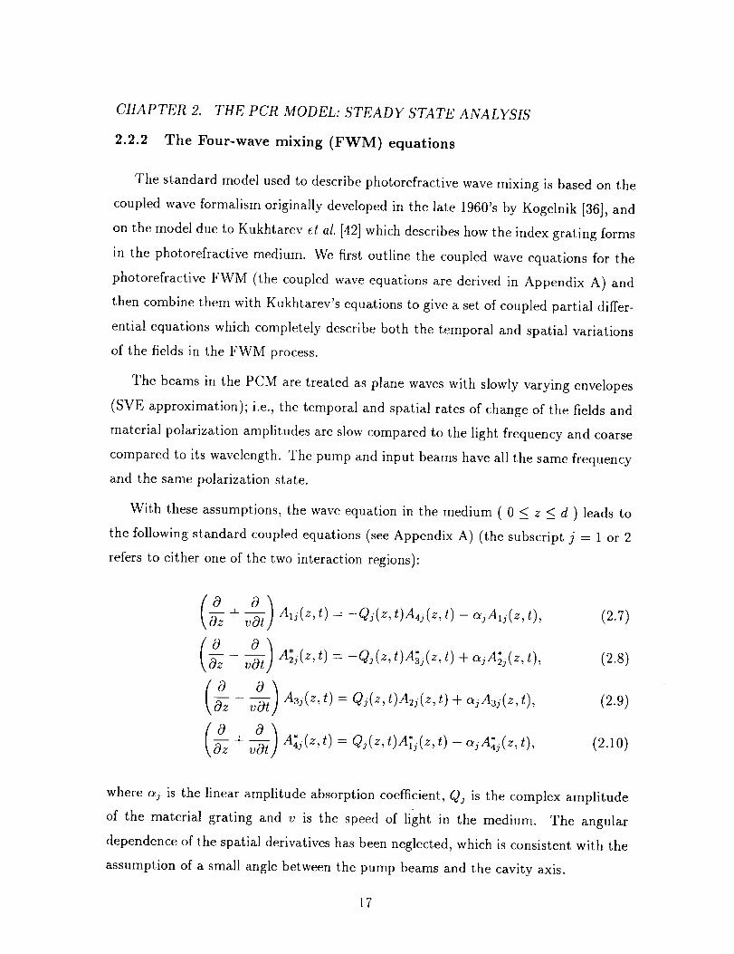
2.2.2 The Four-wave mixing (FWM) equations
The standard model used to describe photorefractive wave mixing is based on the
coupled wave formalism originally developed in the late 1960's by Kogelnik [36], and
on the model due to Kukhtarev et al. [42] which describes how the index grating forms
in the photorefractive medium. We first outline the coupled wave equations for the
photorefractive FWM (the coupled wave equations are derived in Appendix A) and
then combine them with Kukhtarev's equations to give a set of coupled partial differ-
ential equations which completely describe both the temporal and spatial variations
of the fields in the FWM process.
The beams in the PCM are treated as plane waves with slowly varying envelopes
(SVE approximation); i.e., the temporal and spatial rates of change of the fields and
material polarization amplitudes are slow compared to the light frequency and coarse
compared to its wavelength. The pump and input beams have all the same frequency
and the same polarization state.
With these assumptions, the wave equation in the medium ( 0 < z _< d ) leads to
the following standard coupled equations (see Appendix A) (the subscript j = 1 or 2
refers to either one of the two interaction regions):
o)+ -_ Alj(z,t)= -Qj(z,t)A4j(z,t)-ajAlj(z,t),
o)_-Ot A;j(z,t) = -Qj(z,t)A;j(z,t) + ajA;j(z,t),
0] A3j(z,t) = Qj(z,t)A2j(z,t) + c_jAaj(z,t),v-Or/
+ -_j A4j(z,t ) = Qj(z,t)A*_j(z,t) - ajA4j(z,t),
(2.7)
(2.8)
(2.9)
(2.10)
where c_j is the linear amplitude absorption coefficient, Qj is the complex amplitude
of the material grating and v is the speed of light in the medium. The angular
dependence of the spatial derivatives has been neglected, which is consistent with the
assumption of a small angle between the pump beams and the cavity axis.
17

CHAPTER 2. THE PCR MODEL: STEADY STATE ANALYSIS
If the medium response time is much longer than the transit time through the
PCM, as is assumed here, the temporal derivatives can be dropped from the LHS of
equations 2.7- 2.10. The equations then describe a quasi steady state situation in
which the fields' amplitudes follow adiabatically the medium changes.
Futhermore, it was assumed that only one index grating is operative in both
regions. For example, with a geometry utilizing the extraordinary polarization to
take advantage of the large electro-optic coefficient of BaTiO3, the dominant grating
is the one formed by the interference of A1 with A4 and A_ with Aa. Its wave number
is _Cl-/_4 = _ca- k2, where kj is the wave vector of beam j.
The dynamics of the grating formation can be derived from the Kukhtarev equa-
tions and has the following form (see Appendix B where the details of the Kukhtarev
theory and its underlying assumptions are summarized):
O (2.11)"rj-_Qj(z,t) = Qoj(z) - Qj(z,t), j = 1,2,
where Tj is a possibly complex time constant and Qoj is the steady state grating.
These two quantities can be evaluated from the parameters in the Kukhtarev model
as shown in section 2.2.3. From Appendix B, the steady state grating has the form
A_j(z)A*4j(z) + A_j(z)Azj(z)
Q oj (Z ) = "7o3 Iojj = 1,2, (2.12)
where /oj is the local average intensity in region j : Ioj(z,t) = E[Akj(z,t)l _. The
second factor in the RHS of equation 2.12 is the modulation depth of the interference
fringes of beam A1 with A4 and beam A2 with Aa. "roj is the coupling coefficient and
has the form
(2.13)7oj - 4c
where r, H is an effective Pockels coefficient which depends on the geometry and the
18
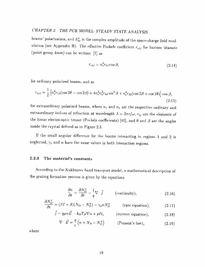
CHAPTER 2. THE PCR MODEL: STEADY STATE ANALYSIS
beams' polarization, and E_c is the complex amplitude of the space-charge field mod-
ulation (see Appendix B). The effective Pockels coefficient r_jj for barium titanate
(point group 4ram)can be written [7] as
4
Fell : noF13 COS _, (2.14)
for ordinary polarized beams, and as
= -- COSr,,, 2 nora3( 20-c°s2/3)+4nenor4zsin2/3+n4r33(cos2/3+cos20 cos/3,
(2.15)
for extraordinary polarized beams, where no and ne are the respective ordinary and
extraordinary indices of refraction at wavelength A = 27rc/w, rij are the elements of
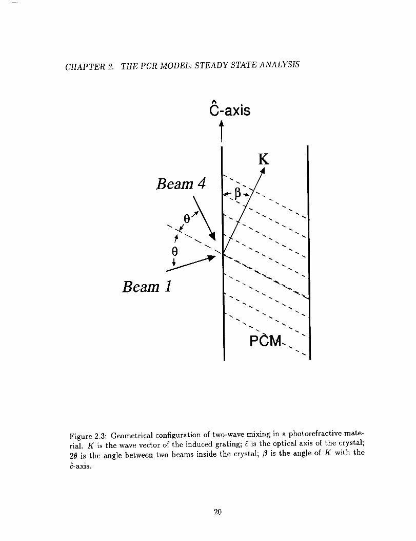
the linear electro-optic tensor (Pockels coefficients) [40], and 0 and/3 are the angles
inside the crystal defined as in Figure 2.3.
If the small angular difference for the beams interacting in regions 1 and 2 is
neglected, 3'0 and o have the same values in both interaction regions.
2.2.3 The material's constants
According to the Kukhtarev band transport model, a mathematical description of
the grating formation process is given by the equations
where
Ot
O_2n ON +D
Ot Ot q_ y
- (SI +/3)(ND -- N+D)--3"RnN +
3 = q#nE, - kBTpVn + pI_c
(continuity), (2.16)
(rate equation),
(current equation),
(Poisson's law),
(2.17)
(2.18)
(2.19)
19
CHAPTER 2. THE PCR MODEL: STEADY STATE ANALYSIS
£;-axis
K
Beam 4
/.O
Beam I
Figure 2.3: Geometrical configuration of two-wave mixing in a photorefractive mate-rial. K is the wave vector of the induced grating; _ is the optical axis of the crystal;
20 is the angle between two beams inside the crystal; fl is the angle of K with the
&axis.
2O

CHAPTER 2.
n(r. t)
Nv
N_(_,t)
J
S
I
7n
#
E
kB
T
P
q
THE PCR MODEL: STEADY STATE ANALYSIS
is the free charge carrier (single species)
number density,
is the total number density of the dopant (single species)
(Fe for example),
is the number density of the ionized donors (traps)
(Fe 3+ for example),
is the number density of the acceptors,
is the number density of neutral (filled)
donors (Fe 2+ for example),
is the current density,
is the photoionization cross section,
is the intensity of the optical wave,
is the recombination rate coefficient,
is the mobility of the charge carriers,
is the total local electric field,
as Boltzmann's constant,
is the temperature,
is the photovoltaic coefficient,
as the charge of the charge carriers, and
as the static dielectric constant.
After linearization in the grating modulation index and in the steady state limit,
equations (2.16)-(2.19) can be solved and the steady state space-charge field is found
to be (see Appendix B):
[(Eo+ Ep)E;c = -iEq [-_o+i-_q + ED)J ' (2.20)
where Eo is the external applied field, Ev, ED and Eq are characteristic fields of the
material:
p/oE_ =
qtmo
kBT[K[E D --
q
(photovoltaic field),
(diffusion field),
(2.21)
21

CHAPTER 2. THE PCR MODEL: STEADY STATE ANALYSIS
(saturation space charge field).qNe
Eq clKI
Here Io is the zero order of the light intensity, N: is the effective trap number density,
K is the grating vector and p is the photovoltaic coefficient [52].
With no external field (Eo = 0) and negligible photovoltaic field (Ep ,-_ 0), the
steady state space-charge field is simply given by
-iEqED (2.22)E;c= Eq + ED"
In this case of a diffusion dominated process, the index grating in equation B.52
leads the light interference fringes by a rr/2 phase shift and the coupling constant
3'0 in equation 2.13 becomes real. The model also predicts a complex response time
constant of the form (see Appendix B)
rg = r_ + i 1, (2.23)_3 9
where the material response time is
(1+ _)2 + (_] 2,,E, (2.24)
and the material frequency is
1 (,_)(_-_/-1)
OJ9 ---- _.]2 2"ra, (1 + ,-D/ + (_)
(2.25)
The various time scales in equations 2.24 and 2.25 are defined by
Td_ --
q#no(dielectric relaxation time),
T_=(_IKIEo)-' (drift time),
(diffusion time),T_ = (_[KIED) -1
(2.26)
(2.27)
(2.28)
22
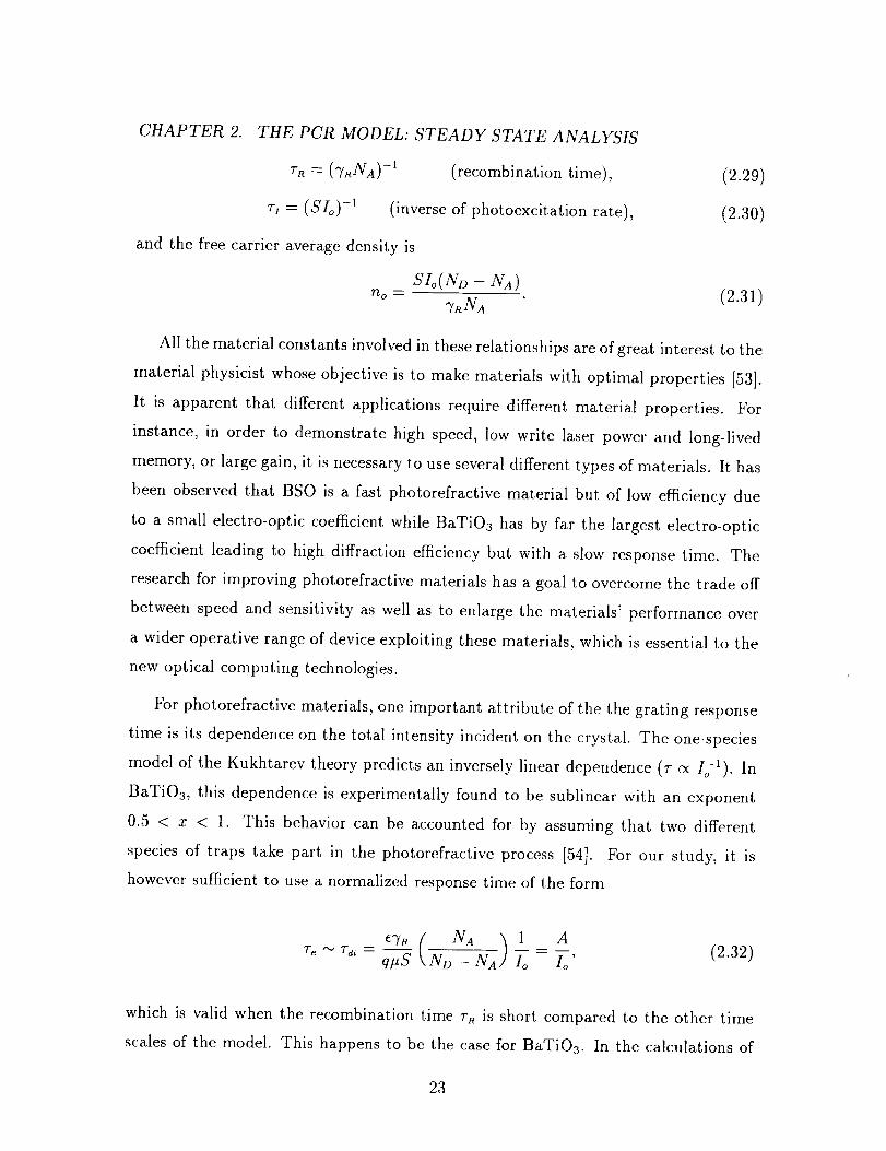
CHAPTER 2. THE PCR MODEL: STEADY STATE ANALYSIS
TR = (7RNA) -1 (recombination time), (2.29)
T, = (SIo)-' (inverse of photoexcitation rate), (2.30)
and the free carrier average density is
SIo(ND- NA)
no = 7RNa (2.31)
All the material constants involved in these relationships are of great interest to the
material physicist whose objective is to make materials with optimal properties [53].
It is apparent that different applications require different material properties. For
instance, in order to demonstrate high speed, low write laser power and long-lived
memory, or large gain, it is necessary to use several different types of materials. It has
been observed that BSO is a fast photorefractive material but of low efficiency due
to a small electro-optic coefficient while BaTiO3 has by far the largest electro-optic
coefficient leading to high diffraction efficiency but with a slow response time. The
research for improving photorefractive materials has a goal to overcome the trade off
between speed and sensitivity as well as to enlarge the materials' performance over
a wider operative range of device exploiting these materials, which is essential to the
new optical computing technologies.
For photorefractive materials, one important attribute of the the grating response
time is its dependence on the total intensity incident on the crystal. The one-species
model of the Kukhtarev theory predicts an inversely linear dependence (7- cx I_-a). In
BaTiO3, this dependence is experimentally found to be sublinear with an exponent
0.5 < x < 1. This behavior can be accounted for by assuming that two different
species of traps take part in the photorefractive process [54]. For our study, it is
however sufficient to use a normalized response time of the form
)1qlaS ND -- NA Io Io'
which is valid when the recombination time rR is short compared to the other time
scales of the model. This happens to be the case for BaTiO3. In the calculations of
23

CHAPTER 2. THE PCR MODEL: STEADY STATE ANALYSIS
the next chapter, we used a normalized time scale 7-o = lo 1. This normalized time
scale can be related to the real time scale for a particular material by evaluating the
constant A. Typical numbers for BaTiO3 are given in Ref. [53]:
S(ND - NA)
7a = 5 x lO-Scma/s,
NA "_ 2 x 1016cm -3,
# ,._ 0.5cm2/V.s,
a _ 0.3cm -1,
q = 1.6 x 10⁻¹⁹C,
eo = 8.85 x 10⁻¹⁴Fcm -1.
(2.33)
The relative dielectric constant is given by
eR = ell sin 2/3 + e± cos 2/3, (2.34)
with ql = 4300, e± = 168 and/3 is the angle between the grating wave vector and the
c-axis of the crystal (Figure 2.3). For the experiment we had /3 ,-- 10 °, which gives
eR _ 300. With these numbers, we find A = 1.1 × 10 is cm -2.
In equation 2.32, Io is expressed in number of photons per cm 2 per sec. In the
calculations of the next chapter, the unit of intensity was chosen to be 1 mW/mm 2.
At a wavelength )_ = 0.514#m (photon energy = 3.87 × 10⁻¹⁹j), this corresponds to
a photon flux of 2.58 × 10¹⁷s-lcm -2. The normalized time scale used is thus given by
with
to(Normalized) = [Io(in mW/mm2)] -1T(in see)
- A _ ,(2.35)
A'- 1.1 x 10 as _ 4.26(s mW/mm2). (2.36)2.58 x 10¹⁷
2.3 Steady-state analysis
The main reason for seeking an analytic steady state solution to the PCR's equa-
tions is that in the quasi steady state case (slow medium such as BaTiO3) such a
24
CHAPTER 2. THE PCR MODEL: STEADY STATE ANALYSIS
solution can be used (as shown in section 2.4) to define a transfer function from
which the stability of the solution can be analyzed. Furthermore, the steady state
solutions determine the threshold for self-oscillations of the PCR.
2.3.1 Steady-state equations and their solutions
The steady state equations are obtained simply by setting all the time derivatives
equal to zero. At steady state, an analytic solution can easily be found in the case
of nondepleted pumps and negligible absorption, i.e. A](z) = A](O) = A_, A2(z) =
A2(d) = A2, and al,2 = 0. Equations ( 2.7- 2.12) then reduce to
d % . .A33(z) = To [A_A4j(z ) + A_A33(z)] As, (2.37)
A j(z/= To% A:A3j(z/]A; j = 1,2, (2.38)where
Io _ IA,I_ + IA212. (2.39)
The boundary conditions are, from equations ( 2.1- 2.4),
I '_-- ,A41(0) = tmAig(O) + rmAa2(0)e 'c2L
A42(0) ' " "_' i_-2L= rrn_t.31(U)e c
Aa,(d) = A3;(d) = O.
(2.40)
(2.41)
(2.42)
To solve the steady state equations 2.37 and 2.38, one may proceed as follows.
Multiply equation 2.37 by p = A_/A1 and we have
d "Y°IA_I_ [A*4j(z ) + pA3j(z)] P _ A_ (2.43)dz (pA3j(z)) - Io ' AI'
d A*4j(z ) = % 1 To ] [A4j(z) + pAaj(z)] , (2.44)
25

CHAPTER 2. THE PCR MODEL: STEADY STATE ANALYSIS
Adding equations 2.43 and 2.44 and integrating, gives
pA3j(z) + A4j(z ) = [pA3j(O) + A'aj(O)]e "_°z. (2.45)
Substituting this equation into equation 2.43 and 2.44 and integrating, gives, respec-
tively
and
A4J(z)-" IA'I2Io [pA3j(O) + A_j(0)] (e "r°z- 1) + A*aj(O), (2.46)
1&12 [pA3j(O) + A4j(0) ] (e "r°z- 1) + A3j(0).A3j(z)- lop
(2.47)
Using the boundary conditions 2.42 in equation 2.47, we find
e-_°d - 1 12
a3j(0) = P'e-_od + Rp a'4j(O)' Rp = _.
Substituting this in equation 2.40 and 2.41, we find
(2.48)
e -'v°d -- 1
I * a* /,_ i_-2L (2.49)A41(0) = tmAIN(O) + rmP /-142t, o)e _ ,e -'_a + Rp
ande -w°d -- 1
A42(0) = r_mp" a41(O)e i_2L. (2.50)e -'_d + Rp
Equations 2.49 and 2.50 are combined to give
A41(0)- tmAIN(O) (2.51)1-¢/ '
with
and
e -w°a - 1 2= 12n
A2 2Rp= Z
(feedback parameter), (2.52)
(pump ratio). (2.53)
Using this result in equations 2.46 and 2.47 and making use of the relationship
between A42(0) and A41(0) derived in equations 2.49 and 2.50, we finally find the
steady state fields in the crystal (0 _< z _< d):
26

CHAPTER 2. THE PCR MODEL: STEADY STATE ANALYSIS
. e "t°(z-d) -_ Rp (tmAiN(O)_* (2.54)A41(z) = e -'Y°d + Rp t _:_ ) '
A42(z)= r=pe_i__2L(e_°(z-d)+ Rp)(e-_°d- 1)*(tmAzN(O)_I_-,o_+ n_l_ t 7--5 )' (2.55)
Az1(Z) = p" e'Y°(z-d)- 1 (t__Am(O)]'\ (2.56)e-_°d + Rp \ 1--8 I '
,. _i__2L(e _°(z-d)- 1)(e -_°d- i)" (tmAlN(O))A32(z)= rmRp_ I_-_od+ Rpl_ k i _--_ ) (2.57)
The cavity fields and the outputs can then be found by using equations ( 2.54-
2.57) in equations ( 2.1- 2.6).
2.3.2 Threshold for self-oscillation
The PCM steady state reflectivities are defined, from equations 2.3 and 2.4, as
A3j(0) j = 1,2. (2.58)#j- A,4j(O ),
Using equations ( 2.54- 2.57), we find
e -'_°d -- 1
#1 = #2 = # = p* , (2.59)e-_od + Rp
and the feedback parameter takes the form
/_= I_,-,,v 12. (2.6o)
If the two interaction regions share the same pumps, they have equal steady state
reflectivity. In a diffusion dominated medium with a stationary grating, the coupling
parameter 7o is real. The phase of the PCM reflectivity is thus simply the sum of
27
CHAPTER 2. THE PCR MODEL: STEADY STATE ANALYSIS
::L
In
019
m
Qrr19
m_
t-O0
19t_
t-O_
%d=4.0
3
2
I I I I I Illl
0 -3 -2 -1 0 110 10 10 10 10
Pump ratio Rp
Figure 2.4: Steady state PCM reflectivity as a function of the pump ratio for various
values of the coupling parameter
28

CHAPTER 2. THE PCR MODEL: STEADY STATE ANALYSIS
the phases of the pump beams: Arg[#] = q)l(0)-_- ¢2(d), ¢1(0) = Arg[Al(0)], ¢2(d) =
Arg[a2(d)].
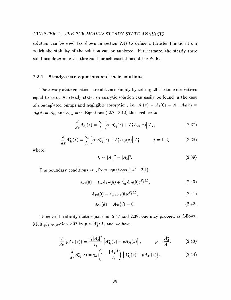
Figure 2.4 shows the magnitude of the PCM reflectivity as a function of the pump
ratio for various values of the coupling constant %d. For the pump ratio Rp << e -_°d,
]#] increases as _p. For Rp >> e -'y°d, t#l drops as 1/_ almost independently of the
coupling constant. Also, the reflectivities all converge to zero as the power of pump 2
becomes much greater than that of pump 1. This is because the index grating written
by pump 1 and the input is erased by the large power of pump 2. Equation 2.60 shows
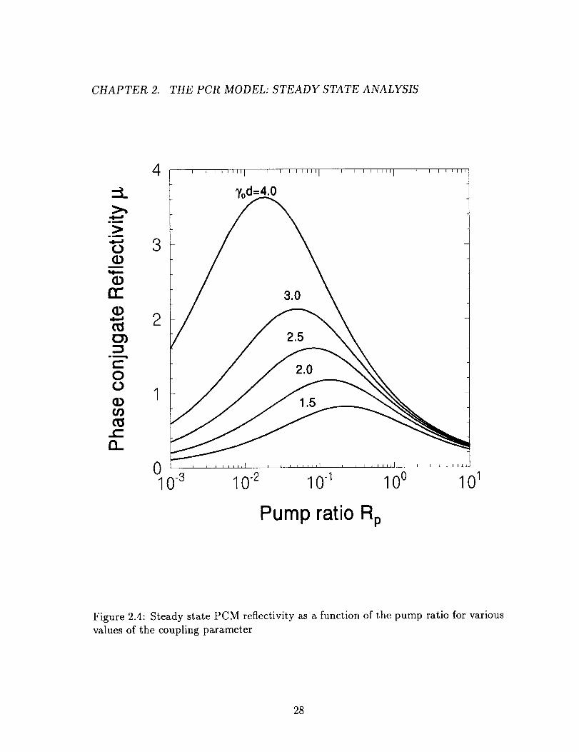
that the feedback parameter is proportional to I#] 2. Care must be taken, however,
in interpreting this result. It is clear that the steady state solution of equations
( 2.54- 2.57) is valid only below threshold, i.e. /3 < 1. The condition/3 = 1, which
corresponds to a feedback system in which the gain exactly compensates the losses,
defines the threshold for self-oscillations of the PCR (i.e. no external input needed
to establish the cavity fields). Figure 2.5 shows/3 calculated from equation 2.60 with
a mirror reflectivity Ir,_l 2 = 0.95. It is seen that for small coupling (7od _- 1.8), the
resonator is stable for the entire range of pump ratios. For larger coupling constant,
there is a range of pump ratios around Rp ,-_ 0.1 which would have/3 > 1. This is
of course not physical. As one approaches threshold, the cavity fields increase, the
undepleted pump assumption ceases to be valid, saturation takes place and 13remains
equal to unity even if the coupling constant is increased.
2.4 Transfer function of the PCR and its stability analysis
In this section, we develop a method to derive a transfer function of the PCR and
we use it for the analysis of the device's frequency response and possible instabilities.
2.4.1 Frequency domain transformation of the PCR's equations
To derive the transfer function, we begin with the time-dependent FWM equations
( 2.7- 2.11) in section 2.2.2. In the undepleted pumps and negligible absorption
29
CHAPTER 2. THE PCR, MODEL: STEADY STATE ANALYSIS
6
4
2
0 0" 3 0- 2 1 0 0 011 1 10 1 1
Pump ratio Rp
Figure 2.5: Feedback parameter as a function of the pump ratio for various values
of the coupling parameter. The steady state solution is valid only below threshold:
8<1.
30

CHAPTER 2.
approximation, they read:
0T-SiQs(z,t)+ Qs(z,t)
THE PCR MODEL: STEADY STATE ANALYSIS
0
+ -_-_) Aaj(z,t) = Qj(z,t)A2, (2.61)
o).v-Or A4j(z't) = QJ(z't)Al' (2.62)
mlA_j(z,t) + A_A3j(z,t)
=70 Io (2.63)
We define a3j(z,_), fi4j(z,_) and qj(z, Ft) as the complex Fourier transforms (or
double sided Laplace transforms) of Aaj(z, t), A4j(z , t) and Qj(z, t), respectively, i.e.
f(ft) =/+5 F(t)e-iatdt' (2.64)
1 [+_+icf(ft)emtda ' (2.65)F(t) = _ J-_+,c
so that 54(z,_) = a_(z,-_). Equations ( 2.61- 2.63) become
Oz + i a3j(z, a) = qj(z,a)A2,
o _-; a4s(z,a) = qs(z,a)A1,
(1 + i_T)qj(z,f_) = _o[Alfi4j(z,f_) + A_aaj(z,f_)].
Thus, the complex amplitudes of a3j and a4j satisfy
[" 63 ._'_ 3'o Ala:j(z,-_)-t- A_a3j(z,_)
+ z v) a3j(z,_) = 1 + iflr Io A2,
(2.66)
(2.67)
(2.68)
(2.69)
._ % Ala_j(z -fl) + A_a3j(z,_) .63 z_) 1 + i_'r Io-_z a*4j( z' -_ ) = ' AI" (2.70)
For a slow medium, the transit time through the PCM is much shorter than
the medium response time (r >> d/v) and the terms ift/v can thus be neglected.
31

CHAPTER 2. THE PCR MODEL: STEADY STATE ANALYSIS
Equations 2.69 and 2.70 are then identical to the differential equations 2.37 and 2.38
used to derive the steady state solutions if the substitution
7o (2.71)V - 1 + i_T'
is made. With a slow medium (v >> cavity round trip time), the boundary conditions
for a3 and a4 also have the same form as equations ( 2.40- 2.42). The solutions of
equations 2.69 and 2.70 are thus identical to the solutions of equations 2.37 and 2.38
respectively, with the substitution of equation 2.71.
2.4.2 Transient response and its stability
From the results of the previous section, we can now define a transfer function for
the phase conjugate cavity beam,
H(_t)a31 (0, _)
m
CtIN(O , _'_)
trap )* e-'_a-1 (2.72)= 1 --_-_) e -'yd + Rp'
with
= I 'l np + np ' (2.73)
where p = A_/A1 and Rp = ]A_/All 2.
From the definition of the complex Fourier transform given in equations 2.64
and 2.65, the system is unstable when the transfer function has poles with negative
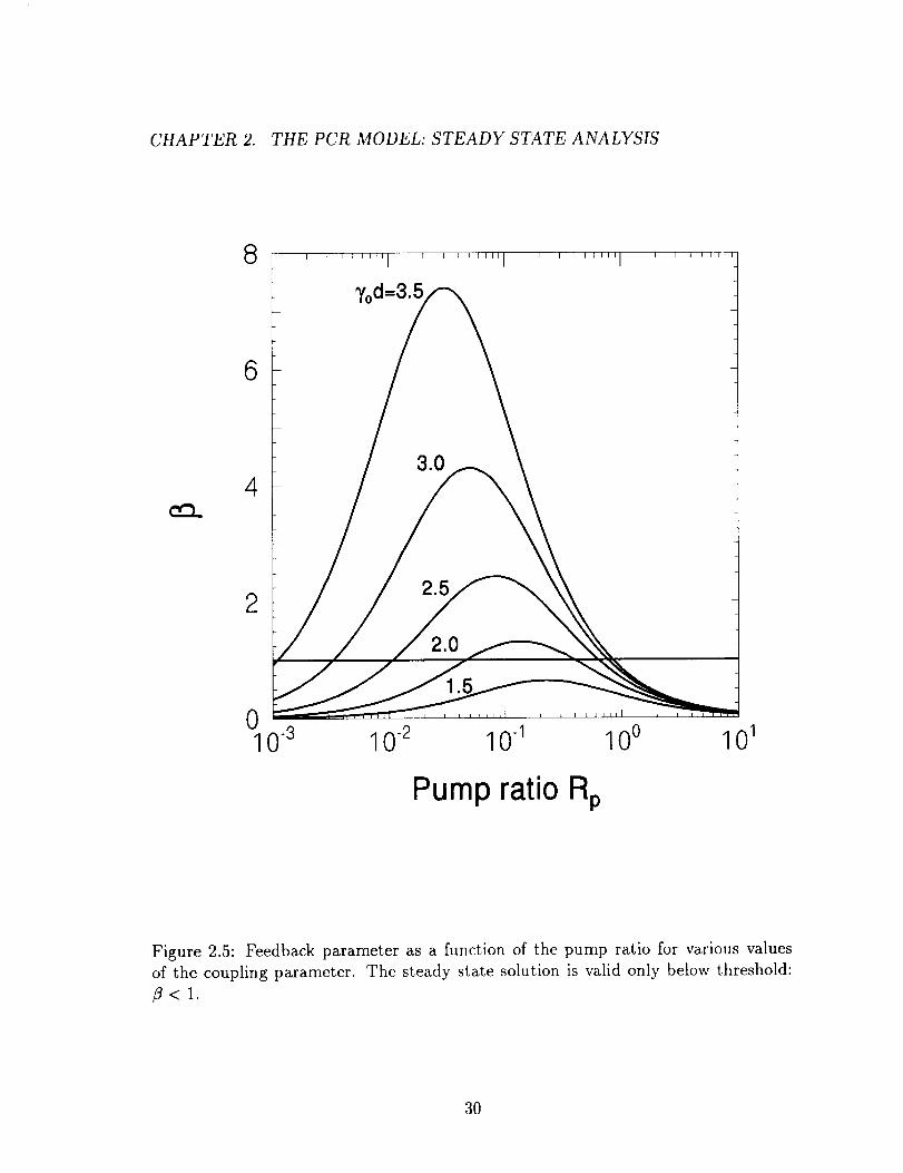
imaginary parts. Figures ( 2.6- 2.8) show contour plots (on a log scale) and 3D plots
(on a linear scale) of the transfer function for three different values of the coupling
parameter. The shaded areas outline the region in which /3 > 1 and in which the
definition of a transfer function becomes meaningless. The poles are located along
the boundary/3 = 1.
For a weak coupling parameter, all the poles are above the real axis and the sys-
tem is stable (Figure 2.6). From equation 2.73 and the parameter values given in
32

CHAPTER 2. THE PCR MODEL: STEADY STATE ANALYSIS
(a) _" 0.5
15/.... .ogIH(..,-!l
v
IE-- 0
-0.5
-1
6
IIIrr,
-2 -1 0 1 2Re(_)
5
--4
(b) _..._3
_2
1
0
Figure 2.6: (a)Contour plot in the complex plane (log scale) and (b)3D plot (linear
scale) of the transfer function of the PCR with a sluggish medium, in the limit of
negligible absorption and no pump depletion. The relevant parameter values are
7od = 1.0, Rp = 0.1, Rm = 0.95. The shaded region outlines the domain/3 > 1.
33

CHAPTER 2. THE PCR MODEL: STEADY STATE ANALYSIS
(a)
1.5
v
E- 0
-0.5
-1-2 2
8O
IoglH(D'c)li i I I _ I i I I i r i i I t q i J
i
-1 0 1Re(_:)
Figure 2.7:
6O
(b) _40.1-
--20
10
Im(l?T)
Same as Figure 2.6 with %d = 2.0. The cavity has just reached threshold.
34
CHAPTER 2. THE PCR MODEL: STEADY STATE ANALYSIS
.5 r i ] r
1
i(a) E 0
-0.5
IO0
-2
loglH(D'OI
-1 0 1Re(@t
r i i
i
2
80m
"_"60(b) CI
"r'__.40
2O
0
Figure 2.8: Same as Figure 2.6 and 2.7 with "7od = 3.0 showing additional unstableconjugate pairs of poles.
35

CHAPTER 2. THE PCR MODEL: STEADY STATE ANALYSIS
the caption of Figure 2.6, it can be calculated that the intersection of the bound-
ary _ = 1 with the imaginary axis crosses to the lower half plane for %d = 1.87
(Figure 2.7). This is, of course, precisely the coupling parameter needed to reach
threshold for these parameter values, as can be verified in Figure 2.5. At this point,
the resonator self-oscillates and has a stable steady state output. As the coupling
parameter increases further, additional complex conjugate poles may cross the real
axis and become unstable. (Figure 2.8).
2.5 Conclusion
We have presented a model and the steady state analysis of the PCR in the
framework of the plane wave representation. A steady state analysis of the FWM
process of the PCR is performed and analytic solutions are derived in the case of
nondepleted pump, an absorption free medium and real coupling constant. Stability
analysis of the solutions is also discussed with the use of the transfer function in
the frequency domain. We find that dynamic instabilities start to come in when the
resonator self-oscillates, i.e. when the feedback parameter _ = 1.
36
Chapter 3
Transient behavior of a PCR:
numerical study
The theory of the photorefractive phase conjugate Fabry-Perot cavity formulated
in chapter 2 was used to find steady state solutions. The analytic results and the
analysis of the stability under quasi steady-state conditions have been presented in
that chapter. For practical applications, it is also crucial to understand the transient
dynamics of the device. In this chapter, the transient regime of a PCR under the
plane wave assumption is studied numerically. In particular we are concerned with
the cavity's response time as a function of the system's parameters. In section 3.1 we
review the time-dependent equations for the waves in a PCR and describe a numerical
method for their solution. In section 3.2 we present the numerical results as functions
of the coupling parameter, the pump ratio, the probe ratio, the dielectric mirror's
reflectivity, and the absorption constant of the medium. The general trends are
discussed in view of the possible use of the system in image processing. In section 3.3
we describe an experimental setup used to study the transient dynamics of a PCR
and discuss the experimental results. A summary of the study is given in section 3.4.
37

CHAPTER 3. TRANSIENT BEHAVIOR OF A PCR: NUMERICAL STUDY
3.1 A numerical approach
In this section we begin with the time-dependent equations derived in chapter 2,
including the pump depletion and medium absorption. We then apply an adiabatic
elimination method to integrate the partial differential equations separately in the
space and time domains to obtain the final steady state of the cavity fields.
3.1.1 The start of the transients
The time-dependent equations derived in section 2.2.2 for the plane wave model
of four wave mixing in a slow photorefractive medium are (figure 2.1):
and
0 t) -Qj(z,t)A4j(z,t) ajAlj(z,t),-_zAlj(Z, =
O A*2j(z,t ) = -Qj(z,t)A_j(z,t) + ajA_j(z,t),
_zA3j(z,O t) = Qj(z, t)A2j(z,t) + ajA3j(z,t),
O A4y(Z,t = Q3(z,t)m_j(z,t) - ajA'4j(z,t),
0 z,t)+Qj(z,t)- 70 • •T--_Qj( io(z,t)[AlJ(z,t)A4j(z, t) + A2J(z't)Aaj(z't)]"
(3.1)
(3.2)
(3.3)
(3.4)
(3.5)
The boundary conditions for the cavity fields are:
A4,(O,t) = tmAiN + r_mA32(O,t) ei-_2L,
A42(0, t) = r_A31(O,t) ei-_2L,
A31(d,t) = A32(d,t) = O,
A,,(0, t) = Al_(0,t)= AIo,
A21(d,t) = A22(d,t)= A2o.
(3.6)
(3.7)
(3.8)
(3.9)
(3.1o)
38
CHAPTER 3. TRANSIENT BEHAVIOR OF A PCR: NUMERICAL STUDY
For the initial state of the PCR, we assume that only the two pump beams A1 and
A2 are present. We further assume that there is no scattered noise so that even if the
cavity is above threshold (gain > loss), self-oscillations do not start spontaneously
without an input beam. Since the interaction between the two pumps is neglected,
their initial spatial distributions in the crystal assume a simple exponential depen-
dence of the form e TM.
The signal beam is then abruptly turned on to a constant value AIN. Since no
interaction takes place yet, it also assumes an exponential distribution:
A41(z,0) : tmA,Ne -oz, (3.11)
A31(z, 0) : A42(z,0): A32(z, 0): 0. (3.12)
After a first short lapse of time, a grating is being formed in region 1, driven by the
interference between A41 and A1 only. The scattering of A2 by this grating produces
a phase conjugate beam Aal. After reflection on the mirror, this beam produces a
probe beam A42 in the region 2. The three beams A42, A1 and A2 in region 2 vary
exponentially in space since there exists no interaction yet, and their interference
triggers the formation of a grating in exactly the same way as in region 1. After a
second lapse of time, this grating generates a phase conjugate beam A32 which adds
up coherently to the input AIN to define the new probe beam A41 in region 1. The
process goes on with the two gratings driving each other's growth and building up
the cavity fields until a steady state is reached.
3.1.2 Adiabatic elimination algorithm
For a slow medium such as BaTiO3, the time derivatives in equations (3.1-3.4)
have been eliminated since the propagation delays in the cavity and in the medium are
short compared with the time needed for grating formation. Under this quasi steady-
state condition, one can regard the field amplitudes inside the crystal as following
the slow grating changes adiabatically. This method was proposed by Heaton et al.
39

CHAPTER 3. TRANSIENT BEHAVIOR OF A PCR: NUMERICAL STUDY
in [17] for the integration of the time-dependent photorefractive equations separately
in the space and time domain and is known as the adiabatic elimination method. The
numerical recipe includes the following steps [55]. At time tN, Qj(z, tN) modulates
the field amplitudes inside the crystal. The spatial distributions of the fields are
calculated by solving the ordinary differential equations (3.1-3.4) with the boundary
conditions (3.6-3.10), by using a fourth order Runge-Kutta method. The boundary
conditions allow one to separate these equations into two independent sets. First,
equations 3.2 and 3.3 are solved simultaneously with the boundary values A3j (d, tN) =
0; A2j(d, tN) -= m2j(O) -= A2o. The solution of this first set of equations is then used
to find the boundary values A4j(O, tN). These, together with the boundary values
Alj(O, tg) = Au(O) = Alo, are used to solve equations 3.1 and 3.4. All the fields
inside the crystal at tg are then known.
The medium then responds to these fields according to equation 3.5 to produce
a new grating Qj(z, tN+l). A second order Runge-Kutta method is used to integrate
this temporal equation, giving
Qj(z, tN+_) .._ Qj(z, tN) + (AtN/r){7omj(z,tN + AtN/2) -- [Qj(z, tN) + (1/2)K(N)]},
(3.13)
where
K (N) = (AtN/T)[%rnj(z, tN) -- Qj(Z,tN)], (3.14)
and
Alj(z, tn)A*4j(z, tN) + A_j(z,tN)Aaj(z, tN)
mj(z, tN) = Ioj(Z, tN) '(3.15)
with tN+l = tN q- AtN. The new grating is then used to find the new spatial distribu-
tion of the fields at time tN+l which is again calculated from equations 3.1 and 3.4.
The process is repeated for a fixed number of steps or until a steady state is reached.
For the calculation to be valid, the time step AtN must be small enough compared
to the time constant T(tN) of the grating. Since this constant is a function of the
4O

CHAPTER 3. TRANSIENT BEHAVIOR OF A PCR: NUMERICAL STUDY
intensity incident on the crystal and therefore changes in time, the temporal step
was not taken as a constant but rather each step was chosen equal to 1/10 the
instantaneous time constant 7(tN) of the grating.
Since, according to the standard Kukhtarev model, the grating time constant is
inversely proportional to the total intensity 11oincident on the crystal, we chose a
relative time scale of the form 7 = I_-1 for the calculations. This time scale can
be related to the actual time scale T = AIo I by evaluating the constant A for a
particular material [53]. Typical values of parameters for BaTiOa give A _ 4.3 s
x mW/mm 2 (see section 2.2.3). The time appearing in the graphs discussed in the
next section is normalized to the medium response time with a total incident Io of 1
mW/mm 2 (e.g., _ 4.3s for BaTi03).
3.2 Numerical analysis
In this section, the numerical procedure just discussed is used to find the transient
behaviors of the cavity fields as functions of the system's parameters. Particular
attention is given to the system response time and the PCR's reflectivity because of
their importance in the design of practical devices.
3.2.1 Response curves for the cavity fields
The system's parameters used in this and the following sections are the coupling
parameter %d, the pump ratio Rp = I2/I1, the probe ratio Rs = ItN/(I1 + h), the
input mirror reflectivity Rm = Irm ]2 and the absorption parameter ad. Figures ( 3.1-
3.5) show the results of sample calculations of the temporal evolution of the cavity
field intensity 131(0, t/To). The other fields experience similar growth. The normalized
intensity of the phase conjugate cavity field intensity I31/(I_ + I2) is plotted as a
function of time, for a square pulse input. The length of the pulse was chosen long
enough to allow the PCR to reach a steady state.
41
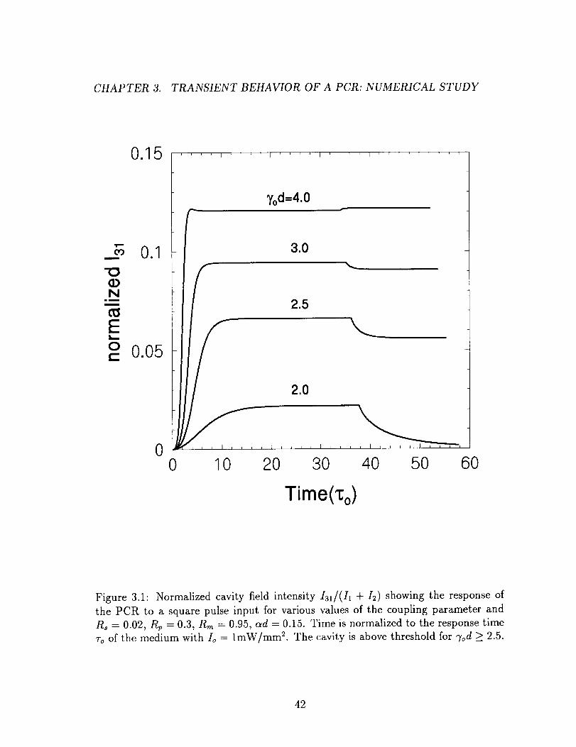
CHAPTER 3. TRANSIENT BEHAVIOR OF A PCR: NUMERICAL STUDY
0.15
m
Nimm
IE
0.1
o 0.05¢..
0
7od-4.0
0 10 20 30 40 50 60
Time(%)
Figure 3.1: Normalized cavity field intensity /Zl/(I1 + 12) showing the response of
the PCR to a square pulse input for various values of the coupling parameter and
R_ = 0.02, R v = 0.3, Rm = 0.95, ad = 0.15. Time is normalized to the response time
To of the medium with Io = lmW/rnm 2. The cavity is above threshold for "/od >_ 2.5.
42

CHAPTER 3. TRANSIENT BEHAVIOR OF A PCR: NUMERICAL STUDY
Figure 3.1 shows the response for various values of the coupling parameter. The
other parameters are Rs = 0.02, R v = 0.3, Rm = 0.95 and ad = 0.15. Larger values
of the coupling parameter lead to larger cavity fields, as expected, to faster growth
rates and to shorter buildup times. For 7od _" 2.2, the cavity is above threshold and a
self-oscillating field remains in the cavity even after the input has been cut off. This
is consistent with the result of figure 2.5 which indicates that at Rp _,- 3, the cavity
reaches threshold for 7od "_ 2 without absorption.
Figure 3.2 shows the response for various pump ratios. In varying Rp the pump
intensity /1 was maintained constant, and I2 was varied. The other parameters are
",/od = 2, Rs = 0.02, Rm = 0.95 and ad = 0.15. With these parameter values, the
cavity remains below threshold for all values of Rv, as shown in figure 2.5. It is seen
that at first, the steady state cavity field intensity increases with increasing pump
ratios and then drops. This is consistent with the result of figure 2.4 which shows
that the PCM reflectivity also reaches a maximum. The buildup and decay rates
follow similar trends but the total buildup time does not vary much with the pump
ratio.
Figure 3.3 shows the PCR response for various probe ratios. The other parameters
are R v = 0.5, ",/od = 2.5, Rm = 0.95, and ad = 0.15. The steady state cavity intensity
increases monotonically with the probe ratio, the buildup rate increases and the
buildup time becomes shorter. The decay time, however, is fairly constant. In this
example, the cavity was slightly above threshold. As the input is cut off, the cavity
field evolves toward a final self-oscillating steady state intensity in a time which does
not depend much on the initial input intensity. This behavior could be found useful
in an optical processor, as it is seen that seeding the PCR with inputs of various
intensities changes the buildup time but does not affect the threshold condition.
Figure 3.4 shows the response for different mirror reflectivies and for %d = 2,
Rp = 0.5, R_ = 0.1. In this case, lowering the input mirror reflectivity increases the
steady-state PCM reflectivity product 1 1 21. Consequently, the increased PCM gain
overcomes the additional losses of the input mirror and leads to a larger steady state
cavity field. The buildup and decay times slowly increase with smaller input mirror
43

CHAPTER 3. TRANSIENT BEHAVIOR OF A PCR: NUMERICAL STUDY
0.025
0.02
COm
"O 0.015(DN
t_
l:::: 0.010¢-
0.005
I I ' ' I
Rp=0.3
0.05
I I
0 20 40 60 80
Time(%)
Figure 3.2: Normalized cavity field intensity I31/(I1 + I2) showing the response of
the PCR to a square pulse input for various values of the pump ratio and %d = 2.0,
Rs = 0.02, Rm = 0.95, ad = 0.15.
44
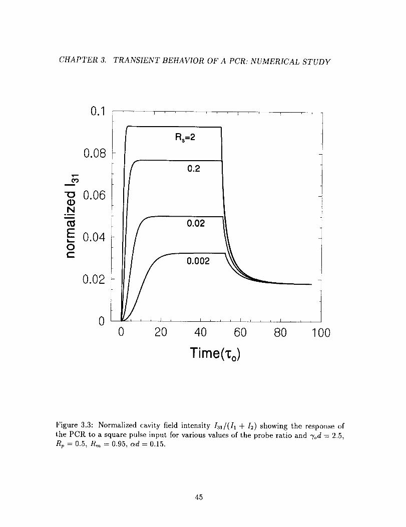
CHAPTER 3. TRANSIENT BEHAVIOR OF A PCR: NUMERICAL STUDY
0.1
,ir...
COm
0N
imm
0.08
0.06
E 0.040
0.02
0
Rs=2
0.02
0.002
0 20 40 60 80 100
Time(%)
Figure 3.3: Normalized cavity field intensity I31/(I1 + h) showing the response of
the PCR to a square pulse input for various values of the probe ratio and 7od = 2.5,
Rp = 0.5, Rm = 0.95, ad = 0.15.
45

CHAPTER 3. TRANSIENT BEHAVIOR OF A PCR: NUMERICAL STUDY
0.05
0.04
0.03N
_0.02
0.01
00
Rm=0.8
0.9
0.95
0.99
I I I I I I i I I I
10 2O 3O 4O
Time(%)
Figure 3.4: Normalized cavity field intensity I31/(I1 + 12) showing the response of the
PCR to a square pulse input for various values of the input mirror's reflectivity and
%d = 2.0, Rp = 0.5, Rs = 0.1, ad = 0.15.
46
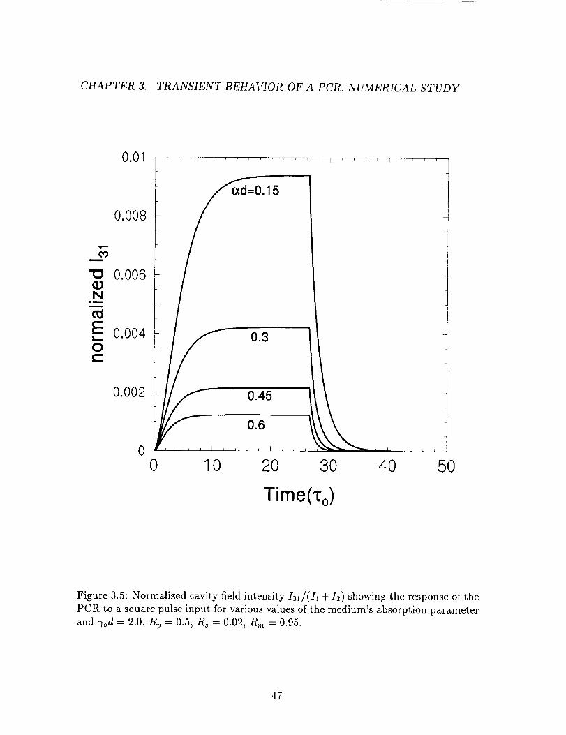
CHAPTER 3. TRANSIENT BEHAVIOR OF A PCR: NUMERICAL STUDY
COm
"OQN
inm
EL_
O¢...
0.008
0.006
0.004
0.002
0
0.45
0.6
0 10 2O 3O 4O 50
Time('to)
Figure 3.5: Normalized cavity field intensity I31/(11 + I2) showing the response of the
PCR to a square pulse input for various values of the medium's absorption parameter
and %d = 2.0, Rp = 0.5, Rs = 0.02, Rm = 0.95.
47

CHAPTER 3. TRANSIENT BEHAVIOR OF A PCR: NUMERICAL STUDY
reflectivity, since this brings the cavity closer to threshold.
Figure 3.5 shows the response for different values of the absorption parameter.
Increasing the absorption losses reduces the cavity field amplitude, everything else
being equal. Here, %d = 2, Rp = 0.5, Rs = 0.02, and Rm = 0.95. The buildup and
decay rates also drop with increasing absorption.
Most of the response curves shown in figures (3.1-3.5) exhibit smooth and mono-
tonic growth to steady state and monotonic decays. With large coupling constant and
especially if the resonator is far above threshold, overshooting and damped oscillations
can also be seen.
3.2.2 Cavity response time
The cavity buildup and decay times were measured from a large number of plots
similar to those shown in figures (3.1-3.5). These times were then plotted as functions
of the pump ratio and the probe ratio, which ratios appear to be the two most
important parameters in determing the system's behavior.
Since some of the buildup curves exhibit overshooting for large "/od, the buildup
time was defined as the time it takes for the cavity intensity to grow from 10% to 90%
of its maximum (which is not necessarily the steady state in case of overshooting).
The decay time was defined as the time it takes for the cavity intensity to drop from
90% to 10% of its steady state value.
Figures 3.6 and 3.7 show the buildup and the decay times, respectively, as functions
of the pump ratio for (a) Rm = 0.8, (b) Rm = 0.95 and Rs = 0.1. For weak
coupling, the buildup time increases with increasing pump ratios for small Rp, reaches
a maximum and drops for larger Rp. This can be correlated with the behavior of the
PCM reflectivity and the cavity field intensity which follow similar trends with varying
Rp, as seen in figures 2.4 and 3.2. For stronger coupling, there is a range of values of
Rp within which the cavity is above threshold. In this region, the initial gain of the
cavity is large (larger than the losses) and the transient buildup is fast, sometimes
48

CHAPTER 3. TRANSIENT BEHAVIOR OF A PCR: NUMERICAL STUDY
0
8
6=m
f:l.:3
!
"13
4
2
Pump ratio Rp8 [ ...... _' [ ....... , ...... , ....... , ,
=E64
0
10 -3 10.2 10 1 10° 101
b Pump ratio Rp
Figure 3.6: a Buildup time versus pump ratio for various values of the coupling
parameter and Rm = 0.8, Rs = 0.1, ad = 0.15. For %d >_ 2.5, the cavity is above
threshold for a range of values of the pump ratio around 10 -1. b Same as figure 3.6aexcept that Rm = 0.95.
49
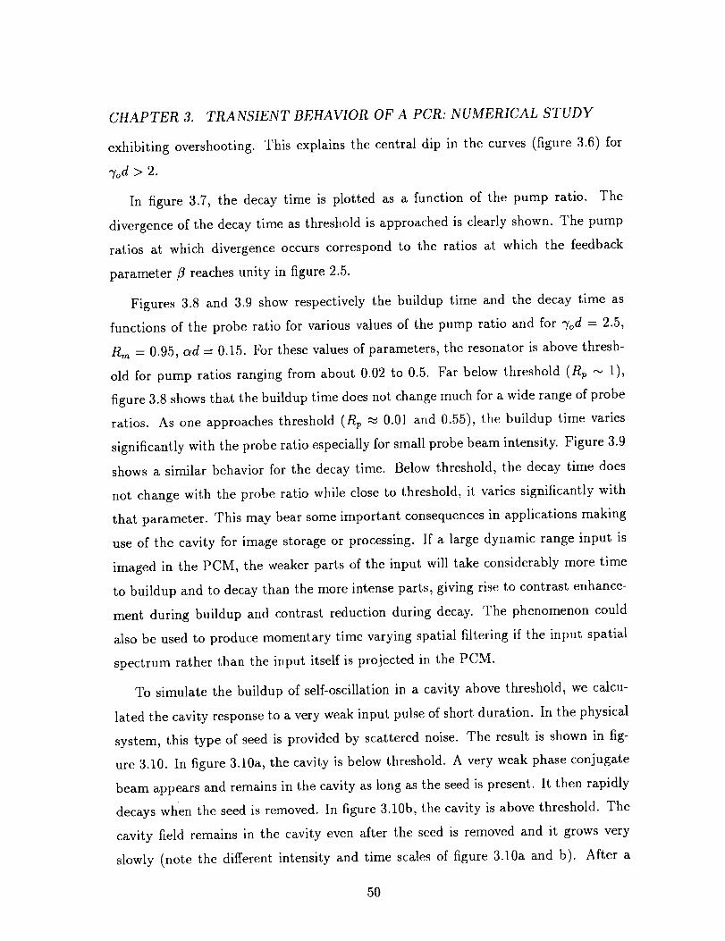
CHAPTER 3. TRANSIENT BEHAVIOR OF A PCR: NUMERICAL STUDY
exhibiting overshooting. This explains the central dip in the curves (figure 3.6) for
7od > 2.
In figure 3.7, the decay time is plotted as a function of the pump ratio. The
divergence of the decay time as threshold is approached is clearly shown. The pump
ratios at which divergence occurs correspond to the ratios at which the feedback
parameter/3 reaches unity in figure 2.5.
Figures 3.8 and 3.9 show respectively the buildup time and the decay time as
functions of the probe ratio for various values of the pump ratio and for %d = 2.5,
Rm = 0.95, (_d = 0.15. For these values of parameters, the resonator is above thresh-
old for pump ratios ranging from about 0.02 to 0.5. Far below threshold (Rp _ 1),
figure 3.8 shows that the buildup time does not change much for a wide range of probe
ratios. As one approaches threshold (R v _ 0.01 and 0.55), the buildup time varies
significantly with the probe ratio especially for small probe beam intensity. Figure 3.9
shows a similar behavior for the decay time. Below threshold, the decay time does
not change with the probe ratio while close to threshold, it varies significantly with
that parameter. This may bear some important consequences in applications making
use of the cavity for image storage or processing. If a large dynamic range input is
imaged in the PCM, the weaker parts of the input will take considerably more time
to buildup and to decay than the more intense parts, giving rise to contrast enhance-
ment during buildup and contrast reduction during decay. The phenomenon could
also be used to produce momentary time varying spatial filtering if the input spatial
spectrum rather than the input itself is projected in the PCM.
To simulate the buildup of self-oscillation in a cavity above threshold, we calcu-
lated the cavity response to a very weak input pulse of short duration. In the physical
system, this type of seed is provided by scattered noise. The result is shown in fig-
ure 3.10. In figure 3.10a, the cavity is below threshold. A very weak phase conjugate
beam appears and remains in the cavity as long as the seed is present. It then rapidly
decays when the seed is removed. In figure 3.10b, the cavity is above threshold. The
cavity field remains in the cavity even after the seed is removed and it grows very
slowly (note the different intensity and time scales of figure 3.10a and b). After a
5O
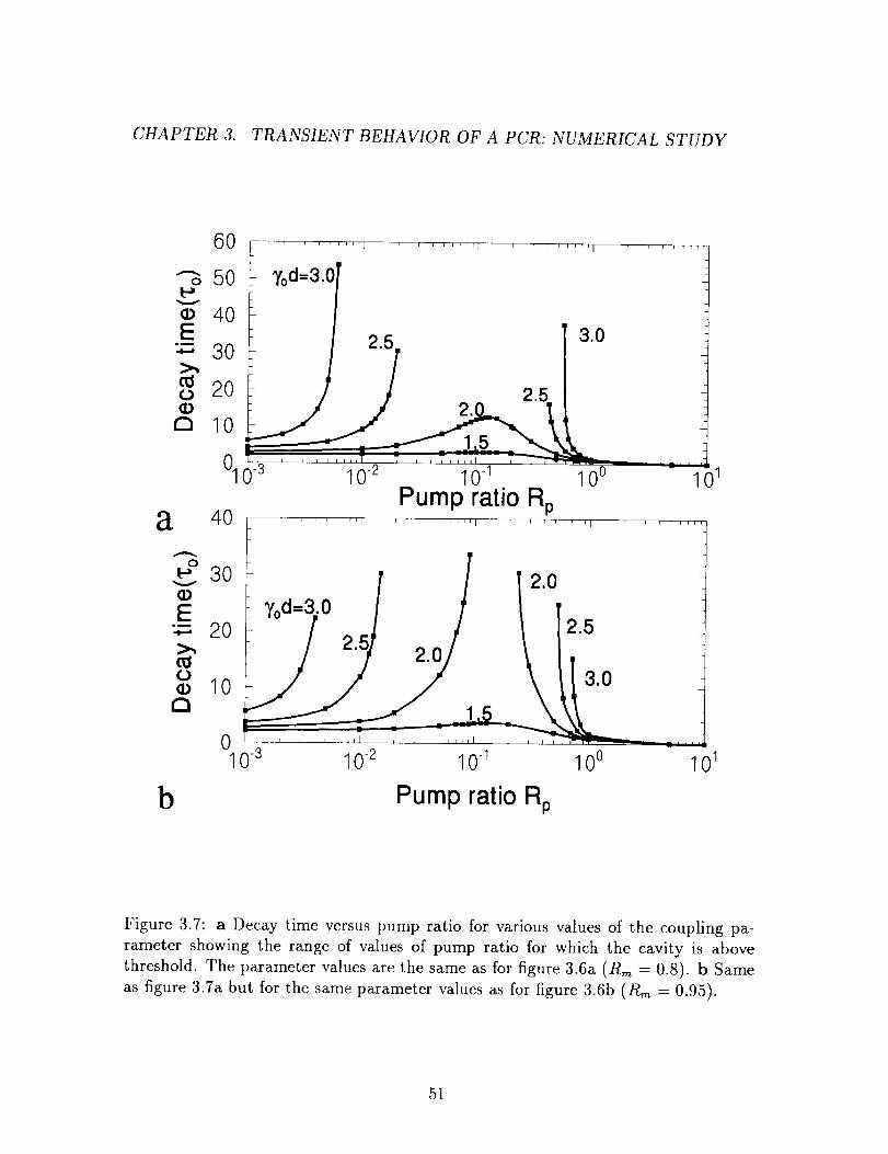
CHAPTER 3. TRANSIENT BEHAVIOR OF A PCR: NUMERICAL STUDY
6O
o 50V
¢_ 40E"_ 30
200
n 10
01
a 40
r i r i _ r_ I I r I , , ,llj I I , , ITT
io -10 " ' ..... 0
Pump ratio RpT _ i r ilfl[ r i I i _ ,,,j , I i r Irlj
_._30
"_ 20
10a
,o.or/ 1,i,,JLX,OZto
L J I J _lJl t L I _ J IIiJ I I I K J iJJ_
10 .2 10-1 100
b
• ' "" ' ' I
10.3 101
Pump ratio Rp
Figure 3.7: a Decay time versus pump ratio for various values of the coupling pa-
rameter showing the range of values of pump ratio for which the cavity is above
threshold. The parameter values are the same as for figure 3.6a (Rm = 0.8). b Same
as figure 3.7a but for the same parameter values as for figure 3.6b (Rm = 0.95).
51

CHAPTER 3. TRANSIENT BEHAVIOR OF A PCR: NUMERICAL STUDY
25
Rp=0.01_ 2O
IE 0.o15im
15!
"Om
"5 10m
50.75
0 0 3 0- 2 0 1 00 012xl 2xl 2xl 2xl 2xl
Probe ratio Rs
Figure 3.8: Buildup time versus probe ratio for various values of the pump ratio and
7od = 2.5, ad = 0.15, R,_ = 0.95.
52
CHAPTER 3. TRANSIENT BEHAVIOR OF A PCR: NUMERICAL STUDY
70, i r ,q, I r i , i E ,ll r r _ r i r ,r_ I i , , ITI
20
10
0.01
0.005 0.75 .0
02x10 -3 2x10 -2 2x10 -_ 2x10 ° 2x10 _
Probe ratio Rs
Figure 3.9: Decay time versus probe ratio for various values of the pump ratio and
the same parameter values as for figure 3.8.
53
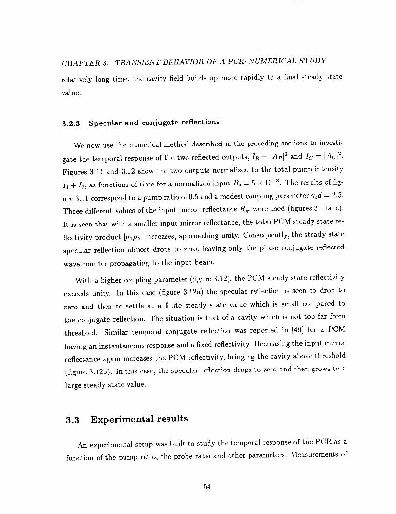
CHAPTER 3. TRANSIENT BEHAVIOR OF A PCR: NUMERICAL STUDY
relatively long time, the cavity field builds up more rapidly to a final steady state
value.
3.2.3 Specular and conjugate reflections
We now use the numerical method described in the preceding sections to investi-
gate the temporal response of the two reflected outputs, In = IARI2 and Ic = IAc] 2.
Figures 3.11 and 3.12 show the two outputs normalized to the total pump intensity
I1 + I2, as functions of time for a normalized input Rs = 5 x 10 -3. The results of fig-
ure 3.11 correspond to a pump ratio of 0.5 and a modest coupling parameter %d = 2.5.
Three different values of the input mirror reflectance Rm were used (figures 3.11a-c).
It is seen that with a smaller input mirror reflectance, the total PCM steady state re-
flectivity product I/_1#21 increases, approaching unity. Consequently, the steady state
specular reflection almost drops to zero, leaving only the phase conjugate reflected
wave counter propagating to the input beam.
With a higher coupling parameter (figure 3.12), the PCM steady state reflectivity
exceeds unity. In this case (figure 3.12a) the specular reflection is seen to drop to
zero and then to settle at a finite steady state value which is small compared to
the conjugate reflection. The situation is that of a cavity which is not too far from
threshold. Similar temporal conjugate reflection was reported in [49] for a PCM
having an instantaneous response and a fixed reflectivity. Decreasing the input mirror
reflectance again increases the PCM reflectivity, bringing the cavity above threshold
(figure 3.12b). In this case, the specular reflection drops to zero and then grows to a
large steady state value.
3.3 Experimental results
An experimental setup was built to study the temporal response of the PCR as a
function of the pump ratio, the probe ratio and other parameters. Measurements of
54

CHAPTER 3. TRANSIENT BEHAVIOR OF A PCR: NUMERICAL STUDY
a
10 -31
"<3
.Nm
Oe--
00
0.02
-- 0.015
QN
0.01
E0 O.OO5¢-
,liTir
5 10 15 20
Time(%)25
0 I I I I J I i J i I , L L ,._ r J i I J
b 0 100 200 300 400Time(%)
Figure 3.10: Response of the PCR to a short seed pulse of intensity corresponding
to Rs = 10 -24. Normalized cavity field I31 versus normalized time for R v = 0.1,
Rm = 0.95, ad = 0.15. a Cavity below threshold with %d = 2.0; b Cavity above
threshold with 7od = 2.2. (Note the different scales).
55
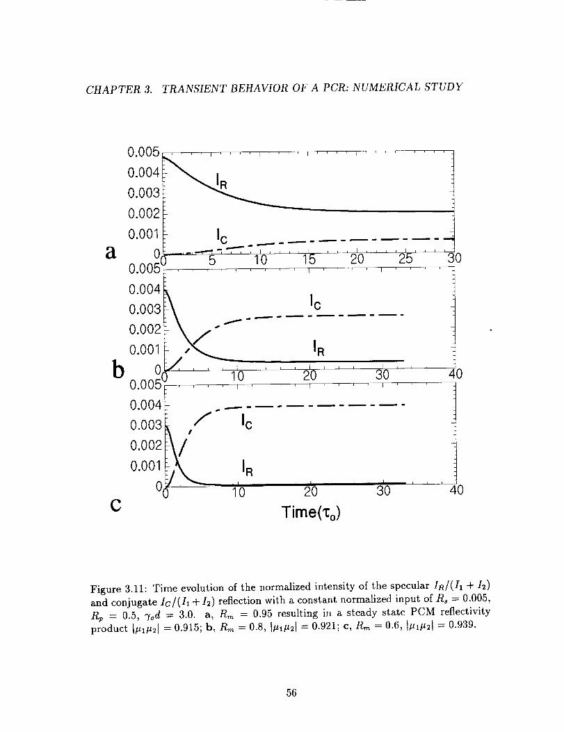
CHAPTER 3. TRANSIENT BEHAVIOR OF A PCR: NUMERICAL STUDY
0.005
0.004
0.003
0.002
I ' 4 I
o.ool Ic _-
a .... :
0.00 '0 ',' ' : ' '
0.004_0.003_-\ _--- IC _.
o0.001 IR
b 0_- .... ' , , 20 ' ,30 ' ' ,400.0050 .... 10
C
0.004
0.003
0.002
0.001
0
f
LIc
IR
10 20 30 40
Time(l:o)
Figure 3.11: Time evolution of the normalized intensity of the specular IR/(I1 +/2)
and conjugate Ic/(I1 + I2) reflection with a constant normalized input of Rs = 0.005,
Rp = 0.5, %d = 3.0. a, Rm = 0.95 resulting in a steady state PCM reflectivity
product 1#1#2] = 0.915; b, Rm = 0.8, 1#1#21 = 0.921; c, Rm = 0.6, 1/21#21 = 0.939.
56
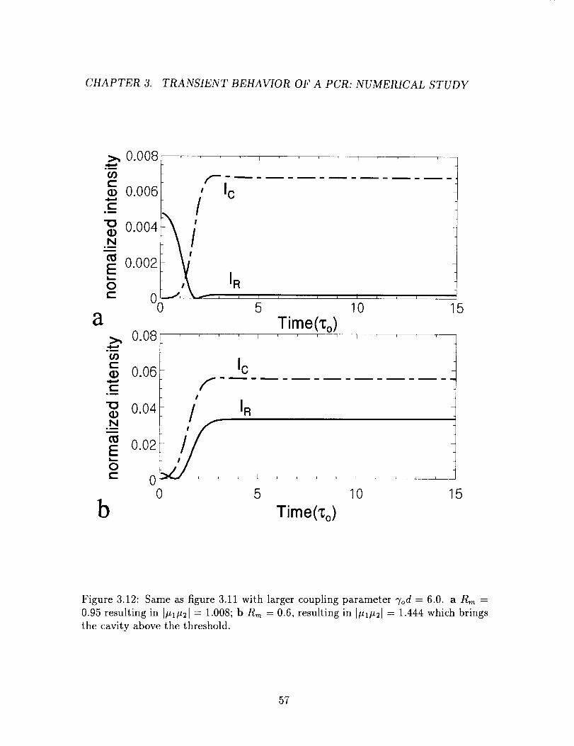
CHAPTER 3. TRANSIENT BEHAVIOR OF A PCR: NUMERICAL STUDY
>, 0.008
t_
0.006
"_ 0.004N
_ 0.002
0oa
>., 0.08.i
cO
0.06
,f" ic
IR
I I
n B j i i [ i i i
5 10 15
Time(%), , F q I ' ' ' ' I ' ' T ,
!
"_N_ 0.04 / In
i 0.02L k L , , , I J
0 5 10
b Time(%)15
Figure 3.12: Same as figure 3.11 with larger coupling parameter "7od = 6.0. a R,, =
0.95 resulting in 1#1#21 = 1.008; b Rm = 0.6, resulting in 1#1#21 = 1.444 which brings
the cavity above the threshold.
57

CHAPTER 3. TRANSIENT BEHAVIOR OF A PCR: NUMERICAL STUDY
the cavity's response times are described and compared, qualitatively, with theoretical
predictions in this section.
3.3.1 Experimental setup
A diagram of the experimental setup is shown in figure 3.13. The PCM is an
externally pumped single crystal of BaTiOa. The laser is a single mode Ar +, operating
at )_ = 514nm. The two pump beams and the input beam are each equipped with
a halfwave plate/polarizer assembly used as a variable attenuator. All polarizations
are extraordinary (in the plane of the figure). The pump and the probe beams made
angles of about 49 ° and 15 ° , respectively, with the normal to the crystal surface. The
input mirror (dielectric) had a reflectivity of 95%. It made a small angle with the
input beam in order to produce two distinct interaction regions in the crystal.
The phase conjugate cavity beam was extracted from the cavity by a pellicle beam
splitter PBS having about 5% reflectance. The lens Le reimaged the interaction
regions in the plane of a slit which was positioned to select the cavity beam I31
and isolate it from the other beam I32. The beam intensity I31 was measured by a
photodetector, recorded and stored in a PC. A shutter was used to turn the input on
and off and produce a square pulse, as in the simulation.
3.3.2 Measurement of the cavity response time
Two sets of data were collected - the first for as high a coupling constant as we
could achieve with this particular geometry and the other for a lower coupling con-
stant, spoiled by rotating the crystal by a few degrees. In both cases, the response to
the input pulse was recorded and the buildup time and the decay time were estimatedL
from the curve. A typical experimental record of the cavity field intensity I31 is shown
in figure 3.14.
The results are shown in figures (3.15-3.18). The error bars in these figures
are qualitative and are intended only to give an indication of the level of confidence
58

CHAPTER 3. TRANSIENT BEHAVIOR OF A PCR: NUMERICAL STUDY
EI
ND
,qL IBS
, _/2
B$
P P
M
_,/2
Probe
Pump1
P
Pump2
BaTiO3
D
Figure 3.13: Diagram of the experimental setup. L: Ar + laser (514nm), ._/2-P:
halfwave plate/polarizer assembly, Sh: shutter, M: 95% dielectric mirror, PBS: pellicle
beam splitter, Le: imaging lens, S: slit, D: photodetector.
59
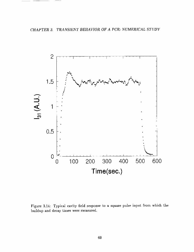
CHAPTER 3. TRANSIENT BEHAVIOR OF A PCR: NUMERICAL STUDY
2 I ' ' I ' ' I ' ' I .... I '
1.5
v
O_m
0.5
00
,%
# •
\
100 200 300 400 500 600
Time(sec.)
Figure 3.14: Typical cavity field response to a square pulse input from which the
buildup and decay times were measured.
6O
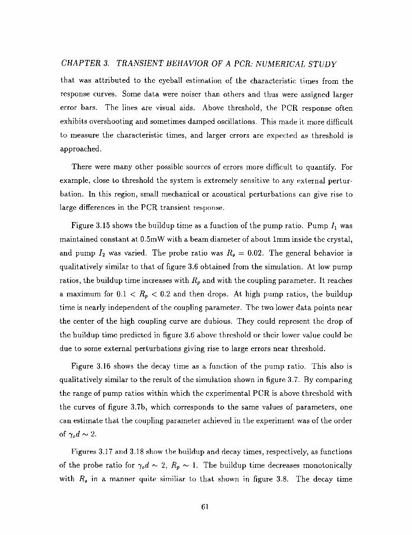
CHAPTER 3. TRANSIENT BEHAVIOR OF A PCR: NUMERICAL STUDY
that was attributed to the eyeball estimation of the characteristic times from the
response curves. Some data were noiser than others and thus were assigned larger
error bars. The lines are visual aids. Above threshold, the PCR response often
exhibits overshooting and sometimes damped oscillations. This made it more difficult
to measure the characteristic times, and larger errors are expected as threshold is
approached.
There were many other possible sources of errors more difficult to quantify. For
example, close to threshold the system is extremely sensitive to any external pertur-
bation. In this region, small mechanical or acoustical perturbations can give rise to
large differences in the PCR transient response.
Figure 3.15 shows the buildup time as a function of the pump ratio. Pump I1 was
maintained constant at 0.5mW with a beam diameter of about lmm inside the crystal,
and pump I_ was varied. The probe ratio was Rs = 0.02. The general behavior is
qualitatively similar to that of figure 3.6 obtained from the simulation. At low pump
ratios, the buildup time increases with Rp and with the coupling parameter. It reaches
a maximum for 0.1 < Rp < 0.2 and then drops. At high pump ratios, the buildup
time is nearly independent of the coupling parameter. The two lower data points near
the center of the high coupling curve are dubious. They could represent the drop of
the buildup time predicted in figure 3.6 above threshold or their lower value could be
due to some external perturbations giving rise to large errors near threshold.
Figure 3.16 shows the decay time as a function of the pump ratio. This also is
qualitatively similar to the result of the simulation shown in figure 3.7. By comparing
the range of pump ratios within which the experimental PCR is above threshold with
the curves of figure 3.7b, which corresponds to the same values of parameters, one
can estimate that the coupling parameter achieved in the experiment was of the order
of %d ,--, 2.
Figures 3.17 and 3.18 show the buildup and decay times, respectively, as functions
of the probe ratio for 7od "_ 2, Rp ,,_ 1. The buildup time decreases monotonically
with Rs in a manner quite similiar to that shown in figure 3.8. The decay time
61
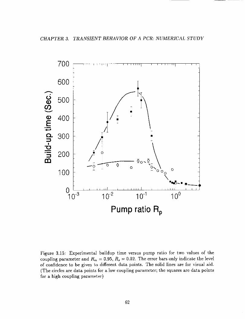
CHAPTER 3. TRANSIENT BEHAVIOR OF A PCR: NUMERICAL STUDY
7OO ' ' ' ''F'_I _ ' ' '''"I , ' ' '''"I , , i
600
d® 500
v
® 400IE
iN
I
m
_m
rn
300
200
IO0o _°"_'__Oo
J I I I I IIIL I L I
10 .2
0
\mmm_" • 0----___
L,ll_i _ i i LLIIII I I J
10-1 100
Pump ratio Rp
Figure 3.15: Experimental buildup time versus pump ratio for two values of the
coupling parameter and Rm = 0.95, R8 = 0.02. The error bars only indicate the level
of confidence to be given to different data points. The solid lines are for visual aid.
(The circles are data points for a low coupling parameter; the squares are data points
for a high coupling parameter)
62
CHAPTER 3. TRANSIENT BEHAVIOR OF A PCR: NUMERICAL STUDY
1500
d¢_ 1000
09v
Q
E
o 500Qa
010-s
l" /
_i j _0 •O_
°°--o<a \
10 .2 10-1 10 o
Pump ratio Rp
Figure 3.16: Experimental decay time versus pump ratio for two values of the coupling
parameter and Rm = 0.95, Re = 0.02. (The circles are data points for a low coupling
parameters; the squares are data points for a high coupling parameter)
63

CHAPTER 3. TRANSIENT BEHAVIOR OF A PCR: NUMERICAL STUDY
behavior is also qualitatively similar to that shown in figure 3.9.
3.4 Conclusion
In this chapter we have presented a numerical scheme for integrating the pho-
torefractive equations separately in the space and time domains using the adiabatic
elimination process. With this numerical scheme, the transient dynamics of a PCR
was described in the limit of a plane wave model and a sluggish photorefractive
medium, but taking into account both the pump depletion and medium's absorption.
The dependence of the cavity buildup and decay times on parameters such as the
pump ratio, the probe ratio, the coupling parameter, the input mirror's reflectivity
and the medium absorption constant were discussed. The numerical results show that
the parameters affecting the threshold most directly are the coupling parameter and
the pump ratio. We find that the higher the coupling parameter, the wider the range
of pump ratio values for which the PCR is above threshold. Results also indicate
that the cavity buildup and decay times can be tailored by varying several of the
system parameters. This may be of importance to image processing applications. For
example, the PCR would, in principle, perform contrast enhancement during buildup
and contrast reduction during decay. This same feature could be used to implement
a time varying spatial filter if the projected field in the PCM is the spatial spectrum
of an image rather than the input image itself.
The numerical simulations also reveal the unusual reflection property of a phase
conjugate Fabry-Perot. For example, we find that when the steady state value of the
phase conjugate reflectivity approaches unity, the specular reflection is completely
extinguished, leaving only the phase conjugate reflection output.
An experimental setup was built to study the transients in a PCR and the exper-
imental results are in general qualitative agreement with the results of the numerical
simulations. In real situations, the material's parameter values may vary considerably
between crystals. In our case, the parameter values for the BaTiOa crystal are cho-
sen from the literature [53]. Futhermore, it seems likely that quantitative agreement
64

CHAPTER 3. TRANSIENT BEHAVIOR OF A PCR: NUMERICAL STUDY
d19
O9V
19
Emm
::3I
"13im
::3
rn
6O
40
20
0 '2x 10.3
\
I\
e d n J eli F I k J L I JJl I I I I J a Ill I J n I _ I a
2x10 -2 2x10 -1 2x10 ° 2x101
Probe ratio Rs
Figure 3.17: Experimental buildup time versus probe ratio for Rp = 1, Rm = 0.95.
65

CHAPTER 3. TRANSIENT BEHAVIOR OF A PCR: NUMERICAL STUDY
d_D
09V
Eli
t_O
a
500 , , ,'""l , ,,,,,,I ' ' '"'"_
4O0
30O
20O
100
02x10 -3
I l I I II t
+
"
I I I Illl I , , , ,_,1 , i i i L illl i _ i _ _ IlL
2xl 0 .2 2xl 0_ 2xl 0° 2xl 0_
Probe ratio Rs
Figure 3.18: Experimental decay time versus probe ratio for Rp = 1, Rm = 0.95.
66
CHAPTER 3. TRANSIENT BEHAVIOR OF A PCR: NUMERICAL STUDY
would require some refinement of the simplified Kukhtarev model by including, at
least, multiple species of traps taking part in the photorefractive process.
67
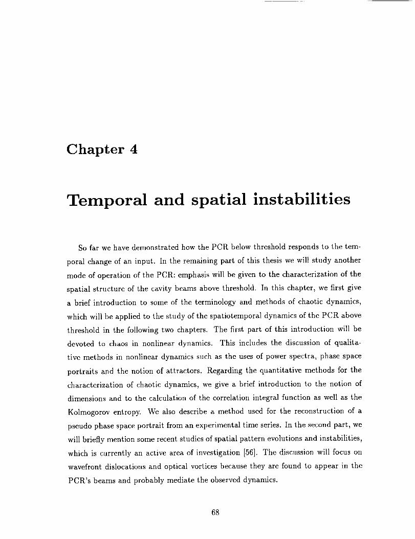
Chapter 4
Temporal and spatial instabilities
So far we have demonstrated how the PCR below threshold responds to the tem-
poral change of an input. In the remaining part of this thesis we will study another
mode of operation of the PCR: emphasis will be given to the characterization of the
spatial structure of the cavity beams above threshold. In this chapter, we first give
a brief introduction to some of the terminology and methods of chaotic dynamics,
which will be applied to the study of the spatiotemporal dynamics of the PCR above
threshold in the following two chapters. The first part of this introduction will be
devoted to chaos in nonlinear dynamics. This includes the discussion of qualita-
tive methods in nonlinear dynamics such as the uses of power spectra, phase space
portraits and the notion of attractors. Regarding the quantitative methods for the
characterization of chaotic dynamics, we give a brief introduction to the notion of
dimensions and to the calculation of the correlation integral function as well as the
Kolmogorov entropy. We also describe a method used for the reconstruction of a
pseudo phase space portrait from an experimental time series. In the second part, we
will briefly mention some recent studies of spatial pattern evolutions and instabilities,
which is currently an active area of investigation [56]. The discussion will focus on
wavefront dislocations and optical vortices because they are found to appear in the
PCR's beams and probably mediate the observed dynamics.
68

CHAPTER 4. TEMPORAL AND SPATIAL INSTABILITIES
4.0.1 Nonlinear systems
In general, the dynamics of physical systems can be described by means of dif-
ferential equations. In cases of nonlinear systems, the equations which govern their
behaviors will contain nonlinear terms. Linearization of the nonlinear terms in some
regions of parameter space where their effects are small often provides simple solutions
and a sufficiently clear picture of the system's dynamics. A classic example of this
is the simple pendulum in the small angle approximation. There are some nonlinear
systems, however, where the nonlinear terms dominate in the physically interesting
region of parameter space. In those cases, the linearization of the system's equations
results in the loss of significant knowledge about the system's behavior. The variety
of responses of nonlinear systems is often found to be much richer than that of linear
systems, as illustrated in figure 4.1 for two systems driven by a sinusoidally vary-
ing input. The output of the linear system must also be sinusoidal, with the same
frequency as the input. The output in the nonlinear system can be periodic (not
necessary sinusoidal); or periodic with subharmonics with frequencies 02/n, where n
is an integer. Another possibility is the occurrence of quasi-periodic motion with an
output of the form cl cos(w,t) + c2 cos(022/), where the ratio 021/022 is an irrational
number if wl and 022 are incommensurate; or the output can be chaotic, fluctuating
erratically in time.
Now, let us look at one example of nonlinear system which is at the origin of
the science of chaos. Chaos was first discovered by E. N. Lorenz [58] in the early
1960s. Lorenz considered a rather typical problem of fluid dynamics which is called
the convection instability or Rayleigh-Benard instability (his purpose was to analyze
the motion of the atmosphere). The motion of the fluid is described by the Navier-
Stokes equations which are nonlinear, partial differential equations. In order to cut
down the complexity of the problem of solving these equations, Lorenz introduced
a Fourier decomposition. He expanded the velocity and temperature fields of the
fluid into spatial Fourier series. The Fourier coefficients were still time dependent
variables. Lorenz truncated the infinite series to only three terms representing three
69
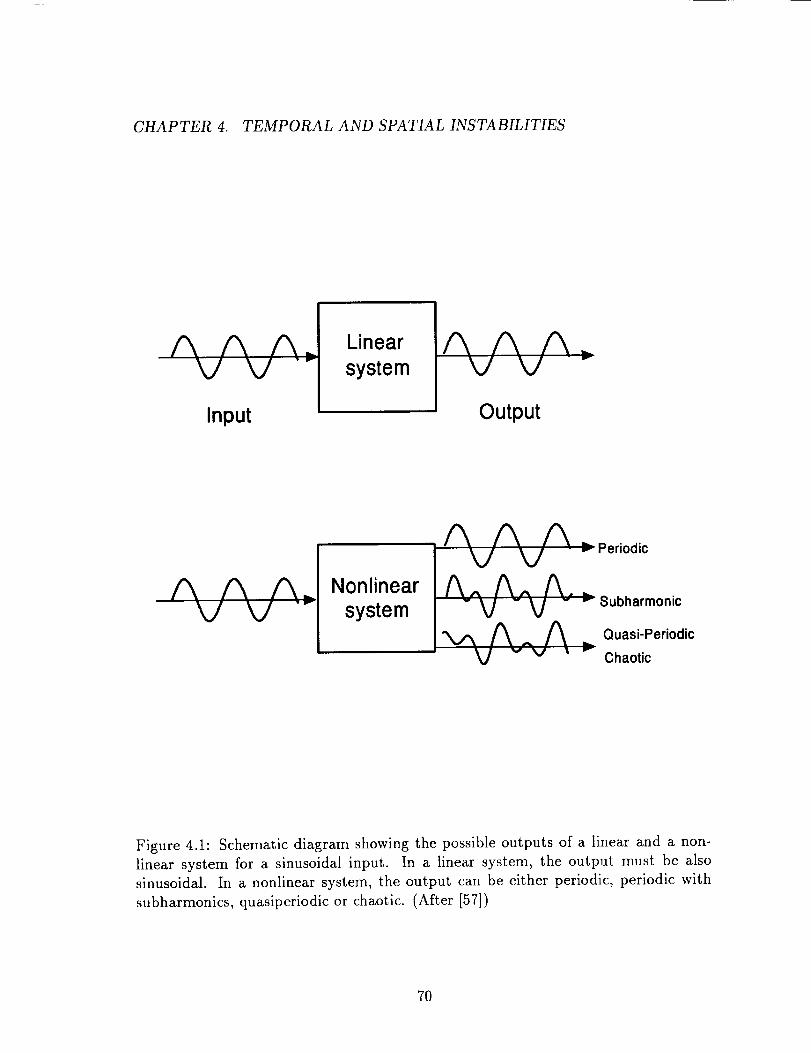
CHAPTER 4. TEMPORAL AND SPATIAL INSTABILITIES
A A A-V V "-
Linear
system
Input Output
A A A-V V '
Nonlinear
system
A A A =Periodick./ kJ
A@@- - " _ Subharmonic
A ^ A ,..Quasi-Periodic
V v _,j _ "- Chaotic
Figure 4.1: Schematic diagram showing the possible outputs of a linear and a non-
linear system for a sinusoidal input. In a linear system, the output must be also
sinusoidal. In a nonlinear system, the output can be either periodic, periodic with
subharmonics, quasiperiodic or chaotic. (After [57])
70

CHAPTER 4. TEMPORAL AND SPATIAL INSTABILITIES
individual modes to save computing effort while still keeping the important physics
of the problem. In this way he derived three coupled differential equations for three
variables. The equations of the Lorenz model are usually written in the following
form:
dX
d--t- = _(Y - X), (4.1)
dY- XZ+rX-Y, (4.2)
dt
dZ
d--t = XY - bZ. (4.3)
X represents the amplitude of the fundamental velocity mode; Y represents the fun-
damental temperature mode and Z represents the temperature second harmonic, a is
the Prandtl number, r = R/Rc is the normalized Rayleigh number relative to the criti-
cal Rayleigh number Rc at which the onset of convection occurs, and b = 4rr2/(_r2+k_),
where kl is a dimensionless wave number. The equations 4.1-4.3 are of quite simple
structure. They are ordinary differential equations and contain only two nonlinear
terms in XZ and XY. To the great surprise of many physicists and mathematicians,
Lorenz found that the numerical solutions for some parameter values (e.g. o" = 10,
b = 8/3, r = 28) can exhibit, in addition to stationary and periodic states, irregular
behaviors. Figure 4.2 illustrates the rapid divergence, characteristic of chaotic behav-
ior, of two solutions which start from initial conditions differing only by about 1 part
in a thousand. Figure 4.3 shows the plots of X versus Y and X versus Z where the
trajectories stay most of the time around certain zones although the trajectories are
never closed.
4.1 Characterization of chaotic dynamics
4.1.1 Fourier spectra
One method of examining the dynamics of a nonlinear system is by Fourier spectral
analysis. Consider the temporal behavior of a function y(t). It is quasiperiodic if its
71

CHAPTER 4. TEMPORAL AND SPATIAL INSTABILITIES
2O
10
X 0
-10
'1 I
iL
II
iI
i I
i q
i I
i L
I
-200 5 10 15 20
-- (X,,Y,,Z,)=(1.0,1.0,1.0)
__ (X,,yo,z,)=(1.001,0.999,0.998 }
Figure 4.2: Graphs of chaotic fluctuations in time of the variable X of the Lorenz's
convective equations. Values of parameters are: a = 10, b = 8/3, and r = 28. This
shows a chaotic solution very sensitive to initial conditions, i.e. two points which
start out close can grow expontentially apart in time.
72
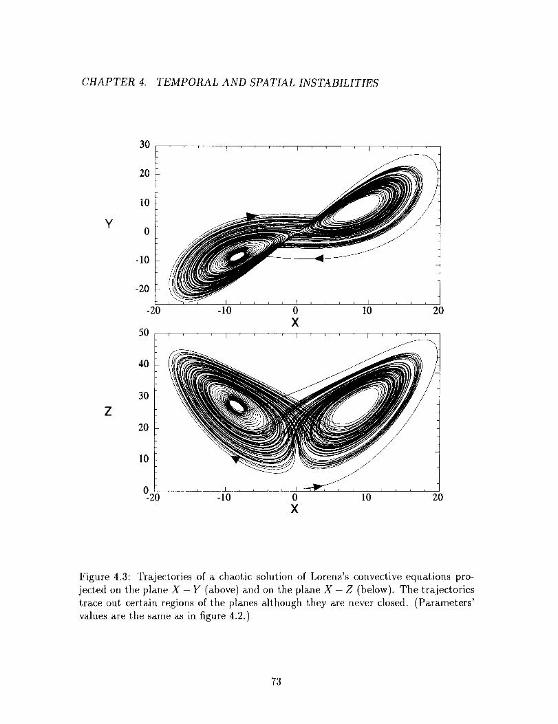
CHAPTER 4. TEMPORAL AND SPATIAL INSTABILITIES
30' I ' ' I i I '
Y
Z
20
10
0
-10
-20
40
30
20
10
-20 -10 0 10 20
X50
0-2t -10 0 10 20
X
Figure 4.3: Trajectories of a chaotic solution of Lorenz's convective equations pro-
jected on the plane X - Y (above) and on the plane X - Z (below). The trajectories
trace out certain regions of the planes although they are never closed. (Parameters'
values are the same as in figure 4.2.)
73
CHAPTER 4. TEMPORAL AND SPATIAL INSTABILITIES
Fourier transform consists of sharp spikes, i.e. if
y(t) = fi cjF "_'t. (4.4)
j----1
The characteristic recurrence feature of quasiperiodicity may be stated formally as
follows: for any _ > 0 there exists a T(_) such that any interval of length T(() of the
real line contains at least one point t' such that ty(t) - y(t')l < _ for any t [59]. Given
y(t), we can always find a t' such that y(t') is as close to y(t) as we wish, and there
are an infinite number of such times t'. Periodic functions are quasiperiodic, but of
course quasiperiodicity does not imply periodicity. Thus the function
y(t) = c, cosset + c2cos 2t (4.5)
is quasiperiodic, but it is not periodic unless wl and w2 are commensurate frequencies,
i.e. unless Wl/_2 is a rational number.
Quasiperiodic motion can certainly look very complicated and irregular, but it
cannot be truly chaotic in the sense of exponential sensitivity to initial conditions. In
particular, the difference between two quasiperiodic trajectories is itself quasiperiodic,
and so we cannot have the exponential separation of initially close trajectories that
is the hallmark of chaos.
Since quasiperiodicity implies order, it follows that chaos implies non-quasiperiodic
motions. Thus chaotic motion does not have a purely discrete Fourier spectrum as
in 4.4, but must have a broadband, continuous component in its spectrum. Fourier
analysis is therefore a very useful tool in distinguishing regular from chaotic motion.
Caution has to be taken here because a broadband spectrum can arise from
stochastic behavior as well as from deterministic chaos. Additional analyses are
therefore needed. For example, for a process governed by stochastic mechanisms,
the spectral power at high frequencies follows a power law. In contrast, for a process
governed by deterministic mechanisms, the power spectrum falls off exponentially [60].
Therefore, a linear behavior on the semilogarithmic plot of a power spectrum indi-
cates that the broadband noise arises from a deterministic rather than a stochastic
process.
74
CHAPTER 4. TEMPORAL AND SPATIAL INSTABILITIES
4.1.2 Phase space portraits and attractors
A dynamical system consists of two parts: the state which describes the essential
information about the system, and the dynamics which is a rule that describes how the
state evolves with time. The evolution can be visualized in phase space, an abstract
space whose coordinates are the components of the state. Therefore, the phase space
provides a powerful tool for inspecting the behavior of chaotic systems. The phase
space represents the behavior in a geometric form. For example, a pendulum that
moves with friction eventually comes to a rest, which in phase space means that the
orbit approaches a stationary point called a fixed point. Since it attracts nearby
orbits, it is known as an attractor.
Some systems do not come to rest in the long term but cycle periodically through
a sequence of states. An example is the pendulum clock (driven pendulum), in which
energy lost to friction is supplied by an external force. The pendulum clock repeats
the same motion over and over again. In phase space such a motion corresponds to
a cycle, or periodic orbit. Such attractors are called limit cycles.
A system may have several attractors. If that is the case, different initial conditions
may evolve to different attractors. The set of points that evolve to an attractor is
called its basin of attraction. The pendulum clock has two such basins. A very small
displacement of the pendulum from its rest position results in a return to rest. With
a larger displacement, however, the clock begins to tick as the pendulum executes a
stable oscillation.
Another type of attractor in phase space is a torus or quasiperiodic attractor,
which resembles the surface of a doughnut. This shape describes motion made up of
two independent oscillating frequencies such as in driven electrical oscillators. One
frequency determines how fast the orbit circles the doughnut in the short direction
and the other regulates how fast the orbit circles the long way around. If motion is
represented by the combination of more than two oscillating frequencies, the attractor
becomes a higher-dimensional torus.
The important feature of a quasiperiodic attractor is that in spite of its complexity
75
CHAPTER 4. TEMPORAL AND SPATIAL INSTABILITIES
it is predictable. Even though the orbit may never exactly repeat itself, i.e if two
frequencies are incommensurate, the motion still remains regular. Orbits that start
on the torus near one another remain near one another, and long term predictability
is guaranteed.
Since the first example of a chaotic or strange attractor discovered by Lorenz, now
known as the Lorenz attractor, interest in looking for this special type of attractor
in phase space has been growing rapidly. A chaotic attractor has a much more
complicated structure than a predictable attractor such as a fixed point, a limit cycle
or a torus. For a chaotic attractor, two orbits with nearby initial conditions diverge
exponentially and then come back close together for only a short time. Stretching and
folding operations which take place in phase space are the key to understanding the
chaotic behavior on these attractors. Exponential divergence is a local feature because
attractors have finite size so that two orbits on a chaotic attractor cannot diverge
exponentially forever. As a result, the attractor must fold over onto itself. Although
orbits diverge and follow increasingly different paths, they eventually must pass close
to one another again. The process of stretching and folding happens repeatedly,
creating folds within folds indefinitely. A chaotic attractor is, therefore, much like
a fractal: an object that reveals more details but self similar as it is increasingly
magnified.
4.2 Dimensions
To distinguish deterministic chaos from stochastic noise, other quantitative means
are needed. A chaotic attractor can be quantitatively characterized by its geometric
properties. A suitable quantity characterizing the attractor as a metric structure is
its dimension.
There are several alternative ways of defining the dimension of a set of points [61].
We shall give what we feel to be the most intuitive one here, called the fractal or
capacity dimension De [62]. Referring to figure 4.4, we consider a set of points
76

CHAPTER 4. TEMPORAL AND SPATIAL INSTABILITIES
N,,., 1/e
N,,.. 1/e2
Figure 4.4: Illustration of the method of covering a 1- and 2-dimensional sets of points
using small squares. This can lead to an intuitive definition of the capacity dimension
(see the text). (After [57]).
77

CHAPTER 4. TEMPORAL AND SPATIAL INSTABILITIES
uniformly distributed along a line as in the above half of the figure. We want to
find out how many small squares of side length c are needed to completely cover the
set of points. If the line is of length l, then this number will clearly be N(e) = I/e.
Similarly, we can consider a two-dimensional set of points as shown in the bottom half
of the figure, and find that the number of small squares needed to cover the area A
is N(e) = A/e 2. Extrapolating this procedure to sets of points in higher dimensions,
we find the following scaling rule:
ldN(e) - -- (4.6)
-- £d'
where d is the dimension of the set of points. From this we can define the capacity
dimension Dc as
log N(¢) (4.7)De = log l + log(i/e)'
and in the limit of small e, the term containing l becomes negligible, i.e.
De "_ limn log N(e) (4.8)0log(1/ )
If the dimension of a set of points as defined in equation 4.7 is non-integer, then the
set is a fractal set.
The structure of the strange attractor does not tell us anything about the fre-
quency with which different points on the attractor are visited in the course of the
flow. It is therefore useful to modify the definition of eq. 4.8 by covering the attractor
with cells and weighting the jth cell by its visitation probability Pj.
information dimension
where
This gives the
DI = limI(e)/log(1/e), (4.9)_---*0
N(e)
I(e) =_- __. Pj log Pj. (4.10)j----1
Note that if each cell has the same visitation probability, SO that Pj = 1/N(c) for all
j, then I(_) = N(e) and DI reduces to De. In general, though, DI <_ De.
To generalize, it is convenient to define an infinite set of dimensions. Let )_(t) =
(xl(t),x2(t),"" ,xd(t)) denote a trajectory in a d-dimensional phase space and con-
struct from the trajectory a sequence of points )_(0), )((T), )_(2r),-..,)_(MT) in
78

CHAPTER 4. TEMPORAL AND SPATIAL INSTABILITIES
phase space, where M is large. Partition the phase space into N(e) cells of side e
and let Mi be the number of points appearing in cell i. Define Pi = Mi/M as the
probability of finding a point in cell i. Then the dimensions D,_ are defined by
Dn=li_ma( 1 ) (_))0 _ log P? /loge. (4.11)
Note that
and
Do = -limlogN(e)/loge = De,¢--*0
(4.12)
D' = li_ma(N_)pil°gPi) /l°ge= Dl'_o \i=1 (4.13)
That is, Do and Da reduce to the fractal and information dimensions defined earlier.
For the total set of generalized dimensions it can be shown that D_ _< Dm for n _> m,
where the equality holds for a completely homogeneous probability distribution, i.e.
P, = 1/N(e). Hence, the difference between dimensions of different order measures the
degree of inhomogeneity of the attractor due to the variation of visitation frequency
of each cell.
The dimension D2 is related to the correlation integral function
C2(e,d) = lim 1 MF_, z,j),i,j=-I
(i_j)
(4.14)
where zij is the separation of two of the points such that z_j = [_d=l(xk(tj) --
xk(tj))_] a/2 and O(x) is the step function such that
(
O(x) = _ 0 , if x<0 (4.15)
( 1 , otherwise.
To see this, note that _ P_ is the probability that any two points lie in the same cell.
This is approximately the probability that two points on the attractor are within a
distance e of each other, which is given by eq. 4.14. Thus, the correlation dimension
is
D2(d) = lim l°g C2(e'd) (4.16)_--.0 log
79
CHAPTER 4. TEMPORAL AND SPATIAL INSTABILITIES
4.2.1 Kolmogorov entropy
Another useful quantity to characterize a chaotic attractor is the Kolmogorov
entropy, which involves a concept with a strong analogy to the entropy concept in
information theory. In information theory, we know that the maximum information
content for a system with two possible states is 1 binary bit. It is 2 bits for a system
with four possible states and so on. In general, the maximum information content is
log_ N bits for N possible states.
Suppose a system has N states, and the ith state is known to occur with probability
Pi. The entropy of the system is defined as
N
S = - _ Pi log_ P,. (4.17)i=1
Here, entropy is a measure of the amount of information necessary to determine the
state of the system. Consider now a trajectory x(t,) = (xl(ti),x2(ti),... ,Xn(ti)) and
partition phase space into n hypercubes of side e. Let P(il,i2,... ,in) be the joint
probability that the point x(ir) lies in the iith cell. Then, from the above discussion,
Kn= y]_ P(il,i2,...,in)log2P(il,i2,...,in ) (4.18)il ,...,in
is a measure of the amount of information necessary to specify the trajectory to within
a precision e. It follows that Kn+l - K,_ is the additional amount of information
required to specify which cell x(nr + T) will fall in. The Kolmogorov entropy may be
defined as [63]
K - limlim a lim ( 1 )
N
,--.o_ og_ -_T y_(li_+l- Iin) (4.19)n=l
= -limlim lim ( 1 )_--.o_--+oN--,oo --_r . ._ . P(il, z2, . . . , in)t1112 _...tln
xlog2P(il,i2,...,i,_ ). (4.20)
We see that K is the average rate of the information loss. Hence, K = 0 in an ordered
system; K = oo in a random system; and K is positive constant _ 0 in a chaotic
8O
CHAPTER 4. TEMPORAL AND SPATIAL INSTABILITIES
system. To generalize, we define the order-q Renyi entropy as
I(q=-limlim lim ( 1 )v---_O_---*ON--*oe Nw(q--1) l°g2 _ Pq(il,i2,...,in), (4.21)il ,i2,...,in
with Pq = Pexp(q - 1)log 2 P. Of all the order-q quantities Kq, I(2 is the easiest
quantity to calculate. It can be shown to be a lower bound to the Kolmogorov
entropy [63].
4.2.2 Dimensions and phase space portraits from an experimental time
series
In the discussion of the preceding section, we made no mention of how one can
construct a phase space portrait of a dynamic system with only time series data for one
variable. For example, in our experiments with the PCR, the data is the temporal
fluctuation of an intensity. According to the Takens embedding theorem [64J, the
topology of an attractor can be reconstructed in an artificial phase space derived
from a single experimental time series. The procedure in such cases is to construct
a pseudo phase space, for example by plotting the value of the measured variable at
time t on one axis and successively time-delayed values on other axes. For example,
we denote the measured quantity at time t by x(t). Then, for a two-dimensional
phase space, we plot x(t + r) on the second axis, where r is a small interval of
time. Construction of a d embedding dimensional phase space follows in the same
manner by using )( = (x(t),x(t + r),..-,x(t + dr)). The choice of r is a debated
subject [56]. There is a certain amount of trial-and-error involved in finding the best
r for a particular problem. If _- is made too large, one loses the correlation between
the data points, with the result that the plot is just a randomly moving wiggly line.
One the other hand, if too small a value is chosen, the plot shows strong dependence
among points and no structure can be resolved.
To calculate the correlation dimension and the Kolmogrov entropy from an exper-
imental time series data, we simply apply the calculation methods discussed in the
preceding sections to the embedding phase spaces made up of those vector points 3_.
81
CHAPTER 4. TEMPORAL AND SPATIAL INSTABILITIES
The second order Renyi entropy is given by
I'(_ = r-'[logC2(e,d)- log C_(e, d + 1)1. (4.22)
For small e and large embedding dimension d it is found that
C2(e,d) " £D2(d) exp(-drK2), (4.23)
so that in practice K2 can be obtained by calculating C2(c, d) for different values of d.
As K2 is a lower bound to the Kolmogorov entropy, the condition Ks > 0 is sufficient
for the existence of chaos.
4.3 Background on spatiotemporal chaos
4.3.1 Extended systems. Weak turbulence
Chaos, as discussed in the preceding sections, is a temporal phenomenon as long
as there are no spatial counterpart involved. This limitation has to be reconsidered
if the degrees of freedom in a dynamical system have a spatial significance. Indeed,
in nonlinear nonequilibrium states, as in fluid convection, there appear structures,
which have been called dissipative structures by I. Prigogine [65]. Examples of these
states having structures include:
(1) patterns with steady structures which vary purely in space (e.g. convection of
fluids, chemical reactions, etc.);
(2) states with homogeneous structures which vary periodically purely in time (e.g.
chemical oscillations, heartbeat etc.);
(3) quasiperiodic states (similar to (2)), which vary quasiperiodically in time;
(4) chaotic states which vary chaotically in time;
(5) turbulent states which vary chaotically both in time and in space.
Some physical systems may only exhibit one of these examples while others can
have all these, such as Rayleigh-Benard convections and Taylor-Couette flows [66].
Regarding the nonequilibrium states involving spatial structures, one of the tasks of
CHAPTER 4. TEMPORAL AND SPATIAL INSTABILITIES
spatiotemporal chaos is to find out how the local/global instability mechanisms are
manifested in the physical space rather than in the phase space portraits.
The notion of temporal chaos discussed in this thesis applies to a situation where
the confinement effects are so strong that the degrees of freedom in a dynamical
system one studies do not have any spatial significance. In that case, one deals only
with the temporal aspect of the dynamics. When systems are weakly confined, i.e. the
boundary effects are less stringent, the instability mechanisms can be then manifested
in the structural modulations. The word pattern will then be a key to the associated
disorder, which has now a space-time meaning.
A much studied example of a confined system is that of a fluid layer contained
in a small box heated from the bottom [67]. At the beginning of the experiment,
the liquid is static. The heat flows across the layer cell via conduction. As the
temperature gradient reaches a critical value, a convection flow sets in. The hot and
less dense liquid rises in the middle while the cool liquid flows down at the sides. So,
there appear two convective rolls. As the temperature gradient is increased further,
the rolls suddenly become unstable in a specific way. A wave (mode) starts running
along the roll (see figure 4.5) periodically. As the temperature gradient is increased
further, an additional new wave (mode) is observed. The temperature monitored
locally fluctuates periodically and quasiperiodically until it becomes chaotic. This
early work has shown how the confinement effects affect the dynamics. From the
physical dimensions of the container, the aspect ratio F can be defined to be the
ratio of the laterial extension l to the height which is comparable to the radii of the
rolls, )_, i.e. F = l/,_. When F is small, the spatial structure is stablized by the
lateral confinement effects. In constrast, when F >> 1, the system is called weakly
confined or extended, where the size of ordered states is down to a local scale only.
The overall structure is then to better understood in terms of pattern or textures. As
the complexity level increases, structural defects may often appear. The role played
by such defects in the turbulent system is a currently active area of research [68].
If now the layer of fluid considered above is contained in a box of much larger
aspect ratios, i.e. the lateral extension is much larger than that of the radii of the
83

CHAPTER 4. TEMPORAL AND SPATIAL INSTABILITIES
T I
Tb
AT:Tb-T t
(To<AT<To,)
(AT>To,)
Figure 4.5: Schematic diagram of the Rayleigh-Benard convection. A thin layer
of fluid in a small box is heated from the bottom. Two convective rolls rotate as
indicated by the arrows when the temperature gradient reaches a critical value. As
the temperature gradient further increases, waves are excited and run along the lateral
direction of the rolls.
84

CHAPTER 4. TEMPORAL AND SPATIAL INSTABILITIES
rolls, a continuous spectrum of excited waves (modes) can be present. When many
of them with comparable wavelength can be present independently with nearly equal
amplitude, their mutual interferences can induce large scale modulations. These
kinds of modulation have been associated closely with the so called the Benjamin-
Feir instability [69]. To describe such modulations or instability mechanisms, the
basic idea of spatiotemporal chaos is to extend the notion of an amplitude that is
time-dependent-only, as in temporal chaos, to account also for spatial dependence.
In other words, the amplitude of the wave has to be described by the two variables
of time and space. In fact, such an idea of using envelop functions for the amplitudes
of the excited waves leads to a complex Ginzburg-Landau equation to describe the
dynamics of the dissipative structures in hydrodynamics [68].
4.3.2 Topological turbulence
The last few years have witnessed very extensive explorations of the spatial be-
havior of laser beams which may display spatial structures similar to those seen in
hydrodynamics [70, 71, 72, 73, 74, 75] . A series of investigations of transverse ef-
fects in laser dynamics by Lugiato and co-workers shows that, just as temporal chaos
results from the presence of at least a few competiting frequencies in a nonlinear
system, instability mechanisms of the spatial structures in a laser may be governed
by the interactions and competitions among a few chosen transverse cavity modes.
The solutions of Maxwell-Block equations including diffraction [70] display families
of transverse patterns containing regularly distributed dark spots called phase singu-
larities [76, 77]. Also, recently, in their analysis of laser cavities with large Fresnel
number, P. Coullet et al. reduced the Maxwell-Block equations to a single equation
of the form of the complex Ginzburg-Landau equation [78]. In the two-dimensional
space of the Ginzburg-Landau equation, they found singular solutions in the form of
spirals. As the spiral waves bear some analogy with the vortices in hydrodynamics,
they are now named optical vortices. In the stable case, these solutions persist in-
definitely owing to their character of topological defect. In the unstable case, they
85
CHAPTER 4. TEMPORAL AND SPATIAL INSTABILITIES
nucleate spontaneously as temporary singularities of the moving wavefront. The spa-
tiotemporal chaotic regime that sets in has been called defect-mediated turbulence
or topological turbulence [79, 80]. Defect-mediated turbulence is currently an active
area of investigation across many disciplines of nonlinear science. The role of de-
fects in mediating turbulence in nonequilibrium systems with large aspect ratios is
an important matter of interest. Therefore, some knowledge of defects [81] becomes
necessary. Before discussing some of the structures and characteristics of defects, let
us close this brief introduction on spatiotemporal chaos with some mention of the
methodologies commonly used for its analysis.
4.3.3 Methodologies of spatiotemporal complexity
At present, there are still no well-established methods for studying spatiotemporal
chaos, in particular the fully developed turbulence. However, we may see emerging
some important paradigms or methods for the study of the spatiotemporal dynamics•
We now describe briefly some of these methods.
One of the oldest examples of a dynamical system which may evolve both in space
and time are cellular automata. Cellular automata were invented in the late 40s by J.
yon Neumann to mimic the behavior of complex, spatially extended structures. W.
Burke gave a good overview of the work of yon Neumann [82]. In cellular automata,
space is divided into discrete small units called cells or sites. The cells take on
numerical values. Consider a one-dimensional cellular automaton consisting of a row
of cells. Each cell is assigned a set of initial numbers. A set of rules specifies how
these numbers are to be changed at every clock step. Suppose that the automaton
initially is filled with 0's except for a single cell which is occupied by a 1:
•..010000000...
And suppose that the rule states that the number in each cell is to be replaced by
the sum of itself and its left neighbor. Thus, after one clock step, the state of the
automaton will be as follows:
...011000000...
86
CHAPTER 4. TEMPORAL AND SPATIAL INSTABILITIES
Another clock step later the state will be
followed by
...012100000...
etc. In fact, this cellular automaton is one of the early yon Neumann machines used
to compute the binominal coefficient of (a + b) '_. Cellular automata can be applied to
one, two and higher dimensional problems. The fixed rules which specify the change
of the cells' values carry out local interactions between neighboring cells, reflecting
the dynamics of the system in question. Cellular automata have been used to model
the complexity in biological systems from the level of cell activity to the levels of
clusters of cells and populations of organisms. In chemistry, cellular automata have
been used to model kinetics of molecular systems and crystal growth. In physics,
they have been used to study dynamical systems such as the clustering of galaxies.
Another model for studying spatiotemporal chaos in spatially extended systems
are the coupled map lattices introduced by K. Kaneko [83]. Coupled map lattices
are dynamical systems discrete in both time and space. Although their modeling
structure looks similar to that of cellular automata, the change of the state of each
site is done by a local mapping function rather than by a set of rules. One example
of coupled map lattices has the form
a:n+,(i) = (1 - D)f(z,_(i)) + D[f(zn(i + 1) + f(x,_(i- 1))], (4.24)
where n represents the time step, i represents a lattice site, and D represents the
diffusive coupling between nearest neighbors. The function f(x) is chosen to be
ax(1-x) (i.e. coupled logistic lattice)or x + A sin(27rx)+c (i.e. coupled circle lattice).
It has been shown that transitions to turbulence via spatiotemporal intermittency
arise in these systems [84]. At the same time, studies of spatiotemporal chaos by
87
CHAPTER 4. TEMPORAL AND SPATIAL INSTABILITIES
coupled map lattices have been growing rapidly because calculations are efficient and
they lend themselves to the generalization of some of the quantitative methods used to
characterize temporal chaos (e.g. Lyapunov spectra and Kolmogorov entropy density
). This approach is also one of the very few known approaches providing means for
the diagnosis of experimental data of spatially extended systems [84].
A third possible approach to the study of spatiotemporal dynamics is called the
modal expansion of fields with transverse structures, as used in laser systems by
Lugiato and co-workers. As is well known, spatiotemporal problems of continuous
variables are mostly described by partial differential equations (PDEs). The solutions
often rely on numerical methods. Sometimes, PDEs can be formidably demanding in
computing power. Lugiato and co-workers demonstrated an alternative way of solving
the PDEs of lasers by expanding the dynamical quantities in a series of normal modes.
The PDEs are then reduced to a set of coupled ordinary differential equations (ODEs)
in the limit of the mean-field approximation. The basic idea of this approach is to
represent the envelop functions of the fields' amplitudes by the space-dependent-only
normal modes and the corresponding time-dependent-only coefficient if it is validly
allowed. This method is highly efficient and yet the essential dynamics of the spatial
structures can still be captured.
A last approach to a description of the turbulent state in a nonequilibrium system
is to characterize it by the presence of topological defects. As mentioned before, this
approach of topological turbulence was first introduced by P. Coullet et al. for laser
systems [80]. They used numerical solutions of the Ginzburg-Landau equation to
illustrate a mechanism of defect formation, annihilation and dynamics in dissipative
structures. Another possible theoretical approach to describe defect formation and
turbulence in large aspect ratio systems has recently been proposed by I. Procac-
cia [85]. In the study of nematic electroconvection, the ordered state of the convec-
tive rolls before the appearance of defects is well described by the envelope equations.
However, how the modulations are affected by the defects is not clear. Procaccia
concluded in his study of nematics that a field theory might be necessary to describe
the dynamics and the interaction forces between defects. On the experimental side,
88

CHAPTER 4. TEMPORAL AND SPATIAL INSTABILITIES
several examples have already demonstrated defect formation in nonequilibrium sys-
tems of large aspect ratios, as in surface waves, in thermal convection, and in the
transverse patterns of lasers and nonlinear optical systems [56, 86]. In fact, the dy-
namics that we observe in the PCR above threshold also provide evidence for such
defect-mediated transitions [87, 88]. This will be demonstrated in the following chap-
ters. But we first introduce in the next section some of the concepts related to the
definitions of defects and in particular the phase defects or wavefront dislocations
observed in electromagnetic waves.
4.4 Wavefront dislocations/phase defects
In this concluding section, we will define the singularities found in electromagnetic
waves and the corresponding terminology used later on in our discussions of the PCR's
dynamics. The discussion given here follows closely that of a paper by M. Berry [89].
Wavefront dislocations or phase defects were first discovered by Nye and Berry
in their study of ultrasound reflected from a rough surface [90]. Wave dislocations
appear ubiquitously in optical fields, acoustics, and quantum mechanics as well as
water waves [81, 91]. Wavefront dislocations are just one kind of singulary that can
appear in scalar waves (for vector or tensor waves, see [92]). Ray caustics are another
kind of wave singularity with a different length scale. On a caustic, rays of light (in a
geometrical optics sense) are all focused to a point and thus the intensity is infinite.
On a phase defect, the intensity is zero. To be observable, the phase defects of a
wavefront must be explored on the wavelength's scale, for example by interferometry.
Caustic singularities, in constrast, are visible to the naked eye (e.g. the reflection of
sunlight from a wavy water surface).
As is well known, singularities are present in many complicated systems, such as
solids, liquid crystals, and hydrodynamics as well as in nonlinear optics. When con-
sidered as geometric structures, singularities are forms rather than materials. Waves
are also forms. Therefore, dislocations in wavefronts are forms of forms. Despite their
"double" abstract nature, they are directly observable phenomena.
89

CHAPTER 4. TEMPORAL AND SPATIAL INSTABILITIES
Another important nature of wavefront dislocations is their singular character.
Consider a travelling wave ¢(r,t) with complex amplitude p(r,t) and phase x(r,t)
defined by
_b = pexp(ix). (4.25)
For the waves in which we are interested, _ is a smooth single-valued function of
position and time. When traversing a loop in the wavefront, X may change by 2mTr,
where m is an integer. Let us shrink the path to a very small loop while the amount
of variation in X does not change. Thus, a singularity is enclosed because X is varying
infinitely fast. And yet the smoothness of _ has to be preserved. It implies that this
can happen only where _ = 0, i.e. X is indeterminate. As _b is null, both Re_b and
Im_b vanish (i.e. Re¢ = Im_b = 0). Thus, phase singularities are points in planes and
lines in space, analogous to crystal dislocations in solids.
Before we illustrate the possible structural forms of the wavefront dislocations by
examples, we would like to ask how they happen. Since the singularities happen only
where _b = 0, i.e. the intensity p2 vanishes, they might be confused with the dark
fringes often discussed in elementary treatments of interference. The dark fringes
are, however, conceived as surfaces rather than lines. Wavefront singularities result
from the destructive interferences of the different rays contributing to _b at a crossing
region of waves scattered from different objects. The crossing can be a point in a
plane or a line in space.
Now we will illustrate some of the possible structural forms of the dislocations of
a wave _ satisfying the wave equation in a uniform static isotropic medium:
1 02_b (4.26)= ;z-by.
Suppose that _ travels only in the z-direction, i.e. _b = p exp(i_), _ = z- ct. The first
case considered is a dislocation moving rigidly with the host wavefront. The wave for
such a case must satisfy
02---_¢+ 02_b - 0. (4.27)= 0u
Consider as an example, _b = A(kx + i/3k_)e ik¢, where A and /3 are real constants.
90
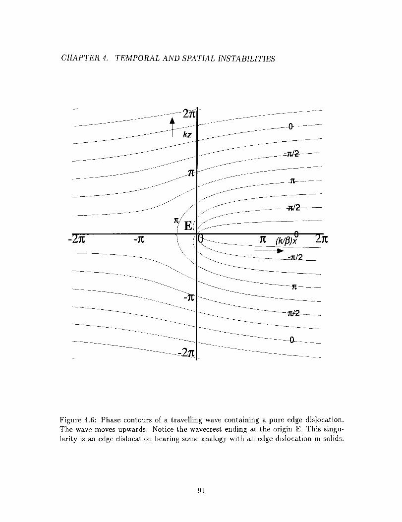
CHAPTER 4. TEMPORAL AND SPATIAL INSTABILITIES
\\
f
J
J
°y
-_at/2_
Figure 4.6: Phase contours of a travelling wave containing a pure edge dislocation.
The wave moves upwards. Notice the wavecrest ending at the origin E. This singu-
larity is an edge dislocation bearing some analogy with an edge dislocation in solids.
91

CHAPTER 4. TEMPORAL AND SPATIAL INSTABILITIES
Figure 4.6 shows the contours of 4, i.e. wavefronts of ¢ moving upwards. The
dislocation is located at E. In crystallographic terms, this is a pure edge dislocation.
The next example of dislocation is the pure screw dislocation, which for strength s
has a wave function
¢ = A(kx + iky)Se ik¢. (4.28)
Figure 4.7 shows the typical plot of pure screw dislocation with strength s = 2.
The sign :k determines the helicity of the screw and the charge s its pitch. Negative
charge of a screw dislocation means that the phase increases counterclockwise around
the dislocation. There is also a mixed type of dislocation, i.e. edge-screw dislocation
with waves of the form
_, = A(kx + ifl(k_ cos_ - kysin _))e _k¢, (4.29)
for example, _ = 0 and _ = 7r/2 correspond to pure edge and pure screw respectively.
Now consider the modulation of the wave in equation 4.25 with quadratic terms in
x, y and which also satisfy equation 4.27. In this way, it would have curved dislocation
lines that move rigidly with the host wave. An example is _ = [(z - iy) 2 + iflk_]e _k_
whose dislocation lines have the form of two parabolas orthogonal to each other, as
shown in figure 4.8a.
We now consider examples showing dislocations moving relative to the wavefront
as the host wave propagates. A simple example of these is
¢ = A[akx + k2x 2 + i(t3k_ + kz)le ik_, (4.30)
where a is real constant. This has two edge dislocations at x = 0 and x = -a/k,
moving parallel to the propagating axis (see figure 4.8b). In a crystallographic term,
such motion is glide. Another kind of movement is made possible if the term in _ is
made quadratic, i.e. if
¢ = A[akx + k2x 2 + i(flk2( 2 + kz)]e 'k_, (4.31)
Now two pairs of edge dislocations are located at x = 0, and x = -a/k. If fl > 0,
members of each pair approach, collide and annihilate while if fl _< 0 they appear and
92

CHAPTER 4. TEMPORAL AND SPATIAL INSTABILITIES
X
1Figure 4.7: Wavefronts of a travelling wave containing a pure screw dislocation. This
helical wavefront with the dislocation along the axis of propagation rotates in clock-
wise. The direction of rotation determines the sign or charge of the screw dislocation.
Clockwise rotation means a positive charge and vice versa.
93

CHAPTER 4. TEMPORAL AND SPATIAL INSTABILITIES
Z
Z
(b)
-at 0
X
Figure 4.8: Examples of dislocations' motion in a travelling wave. The wave travels
upwards (see text for details).
94
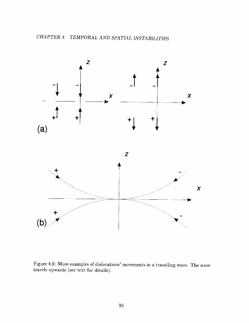
CHAPTER 4. TEMPORAL AND SPATIAL INSTABILITIES
(a)
Z
J +X
Z
X
Z
. ÷\
+ -
m i
\
\\
X
Figure 4.9: More examples of dislocations' movements in a travelling wave. The wave
travels upwards (see text for details).
95

CHAPTER 4. TEMPORAL AND SPATIAL INSTABILITIES
then glide apart (see figure 4.9a). If a slight change of form is made in equation 4.31,
for example, if it becomes
_l, = A[k_x 2 + i(t3- i,,/)k2_ 2 + ikz]e ik_, (4.32)
where 7 is a real constant, two pairs of edge dislocations ap_koach each other along
parabolic trajectories and annihilate when they meet (see figure 4.9b). Such motion,
called climb, corresponds to the spontaneous recovery of a tear in a wavefront. Above
are a few of many possible structural forms and movements that the wavefront dis-
location or phase defects can have. Many other interesting examples can be found in
references [90, 93, 89].
In conclusion, we have presented a brief introduction of nonlinear dynamics and
spatiotemporal as well as temporal chaos. Of particular interest are the definitions
of topological turbulence and the role played by the wavefront dislocations or phase
defects in mediating the dynamics. Some aspects of these phenomena will be illus-
trated in the study of the PCR's dynamics above threshold, described in the following
chapters.
96
Chapter 5
Experiments: spatiotemporal
dynamics in PCRs
In this and the following chapter we present the results of an experimental study
of spatiotemporal structures in the PCR's beams above threshold. In this chapter,
the emergence of spatiotemporal structures as the degree of transverse confinement is
varied by changing the Fresnel number will be described in detail. A theoretical model
of the spatiotemporal dynamics of the PCR will be presented in the next chapter.
This chapter is organized as follows: In section 5.1, the experimental arrangement
for the study of the spatiotemporal dynamics of the PCR will be described. The
experimental results and their analyses are presented in the following five sections.
The dynamics of the local intensity measured at one point in the beam will be analysed
in section 5.2 with the aid of experimental time series, power spectra and phase
space portraits. An attempt at quantifying the chaotic dynamics by calculating the
correlation dimension and the Kolmogorov entropy will be presented in section 5.3.
The spatial instabilities of structures across the PCR's beams will be discussed in
sections 5.4 and 5.5, where it is indicated that the spatiotemporal dynamics observed
has some the characteristics of a topological or defect-mediated turbulence. Finally,
in section 5.6, it is shown that the superposition of a few simple empty cavity TEM
97
CHAPTER 5. EXPERIMENTS: SPATIOTEMPORAL DYNAMICS IN PCRS
modes with different frequencies have a dynamical behavior compatible with the
observed phenomena. Additional discussion and conclusions are presented in the
concluding section 5.7.
5.1 Experimental setup
The linear phase-conjugate resonator under study is sketched schematically in
figure 5.1. The resonator consists of a flat dielectric mirror M (95 % reflectance) and
a phase-conjugate mirror. The phase-conjugate mirror is a single crystal of BaTiOa
5mmx5mmx7mm in size. It is pumped externally by two counterpropagating beams
from a single-mode Argon ion laser tuned to 514nm. The beam diameter is about
1.5mm. The intensity and polarization direction of each pump beam are controlled
independently by assemblies consisting of a half-wave plate and a crystal polarizer.
In all experiments reported in this chapter, both beams' polarization directions were
extraordinary, i.e. in the same plane as the _-axis of the crystal, which lies in the
plane of the figure.
The resonator contains two apertures, H1 and H2. The aperture H2 is located as
close as possible to the mirror M and in the front focal plane of a 16 cm focal length
lens. The aperture H1 is in the back focal plane of that lens, about 3 cm away from
the phase-conjugate mirror. The degree of transverse confinement of the system can
be varied by changing the apertures sizes. A quantitaive measure of this confinement
is given by the resonator Fresnel number defined as
F- DID2 (5.1)
where D1 and D2 are the diameters of the apertures H1 and H2 respectively, A is the
wavelength and f is the focal length of the lens. D1 is small enough to ensure that
the interaction region in the crystal is smaller than the area of pump overlap. The
Fresnel number has a concrete physical meaning [94]. A simple argument based on
scalar diffraction theory shows that the transverse dimension of a speckle near the
aperture H1 is given by Af/D_. F is, therefore, a measure of the number of speckles
98
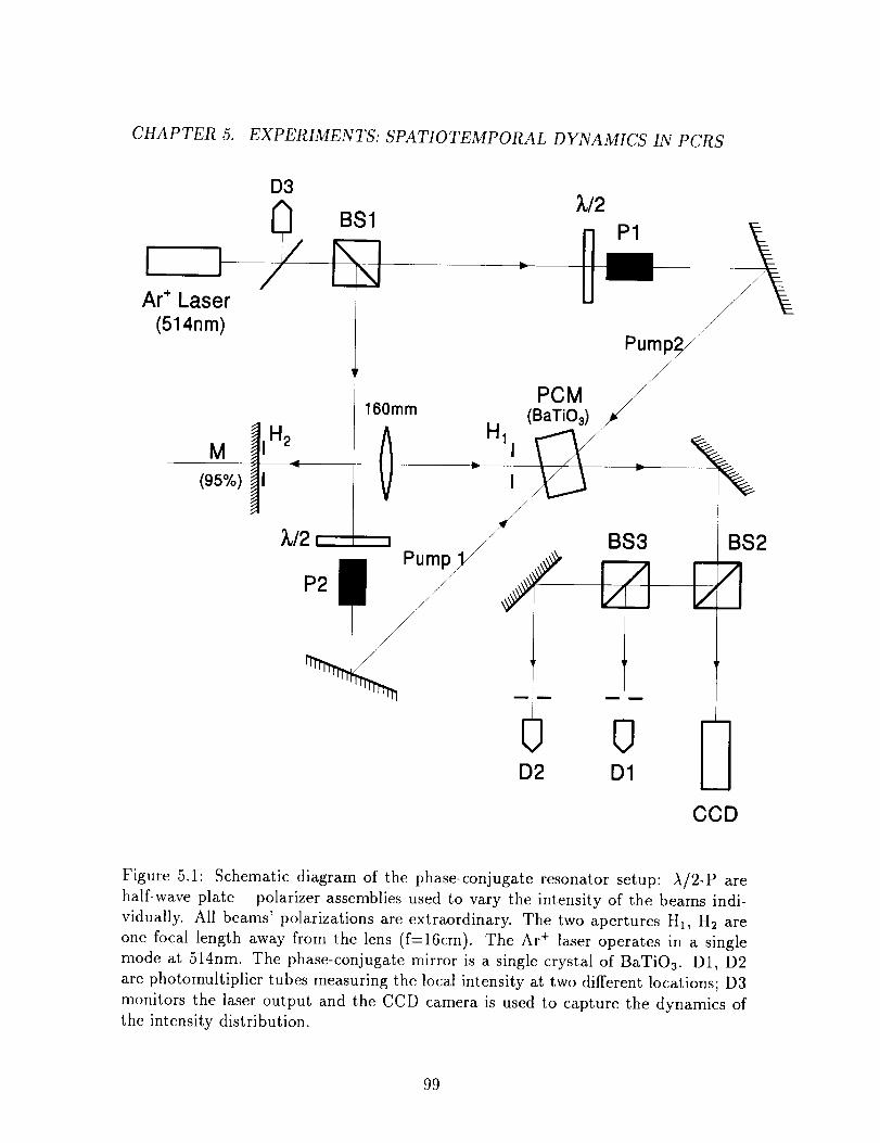
CHAPTER 5. EXPERIMENTS: SPATIOTEMPORAL DYNAMICS IN PCRS
Ar ÷ Laser
(514nm)
D3
M I IH2
(95%) II
BS1
160ram
0
Z/2
PCM /
(BaTiOs)_
I
Z
BS3
J [JD2 D1
Pump/
BS2
CCD
Figure 5.1: Schematic diagram of the phase-conjugate resonator setup: )_/2-P are
half-wave plate - polarizer assemblies used to vary the intensity of the beams indi-
vidually. All beams' polarizations are extraordinary. The two apertures H1, H2 are
one focal length away from the lens (f=16cm). The Ar + laser operates in a single
mode at 514nm. The phase-conjugate mirror is a single crystal of BaTiO3. D1, D2
are photomultiplier tubes measuring the local intensity at two different locations; D3
monitors the laser output and the CCD camera is used to capture the dynamics ofthe intensity distribution.
99

CHAPTER 5. EXPERIMENTS: SPATIOTEMPORAL DYNAMICS IN PCRS
along any transverse diameter in the resonator field. In all the experiments reported
here, except for the measurements made with F < 3 , the aperture H1 was fixed with
D1 = 0.69ram.
The Fresnel number is the control parameter used in the experiments. The Bragg
detuning achieved by misaligning one of the two pumps is another significant param-
eter, which will be considered in the next chapter. Both appear to be the parameters
that most directly affect the spatiotemporal dynamics of the system. Two other pa-
rameters have been observed to affect the dynamics as well, but to a much lesser
degree. The first is the total intensity Io incident on the crystal. The response time
associated with the photorefractive effect is roughly inversely proportional to the in-
tensity in the range used ( 10mW/mm 2 "_ 100 mW/mm _ ). For our crystal, the
response time was of the order of ls mm2/mW. The second factor influencing the
dynamics is the pump ratio, defined as Rp = I2/I1, where/2 and I1 are pump 2 and
pump 1 intensities, respectively (see figure 5.1). The pump ratio can be used to vary
the departure of the cavity from threshold, which affects the buildup and decay rates
of the cavity [34]. It has been seen in chapter 2 that the decay time diverges for
the values of the pump ratio at which the cavity reaches threshold for self-oscillation.
From chapter 3 (fig. 3.10), it is seen that the cavity is above threshold for 0.1< Rp <
1. The departure from threshold can then be varied by choosing a pump ratio within
that range. With a better alignment of the crystal, and thus a higher gain coefficient,
that range could be extended to Rp < 2 for the experiments described in this chapter.
With a tight confinement (F = 1.8), giving a stationary output, we measured the
intensity and the buildup times of the phase conjugate beam/3 against the pump ratio
for various values of the total pump power. The goal was to determine what values of
these two parameters gave rates of change of the observed phenomena compatible with
visual observation and standard video recording. The results are shown in figure 5.2.
For all the experiments reported here, the pump ratio was fixed at 1 and the total
power of the two pumps was kept at 60mW. Other parameters such as alignments,
four-wave-mixing geometry, etc., were fixed for all the measurements.
The field distribution in aperture H1 was imaged (with lenses not shown in Fig. 5.1)
100
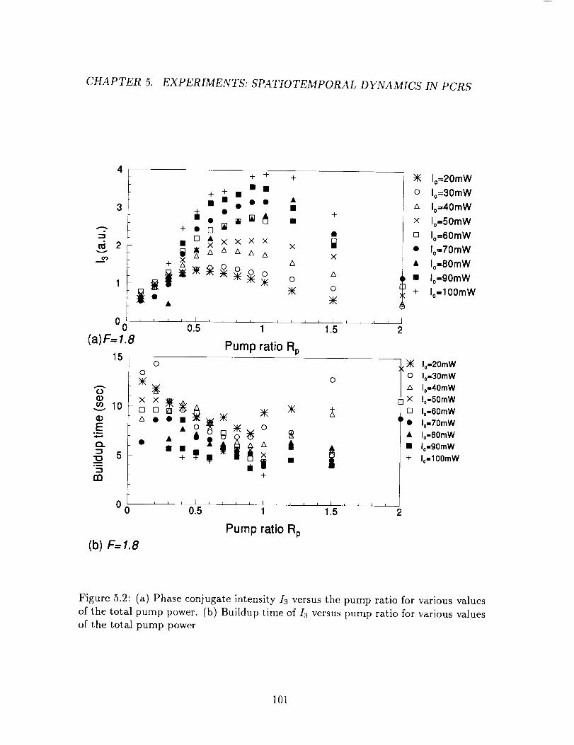
CHAPTER 5. EXPERIMENTS: SPATIOTEMPORAL DYNAMICS IN PCRS
3
O_
1
+ + +
+ + • • •• • • • •
• •
" iio mN •
+ o D _
×_ A A X
o
0.5 1 1.5O0 J J i E 2(a)F-1.8
Pump ratio Rp15
OO
xx_ __ oom
• m • A+)_ n@ •+
oG)
._ 10QE
.b
-.-z"o 5oi
rn
k I I l J i I I i I I J a L J d J L I
0 0.5 1 1.5 2
(b) F= 1.8Pump ratio Rp
Io=20mW
o Io=30mW
z_ Io=40mW
x Io=50mW
[] Io=60mW
• Io=70mW
• Io=80mW
• Io=90mW
+ Io=100mW
Io=20mW
0 Io=30mW
/', Io=40m w
X Io=50mW
[] Io-60rnW
• Io=70mW
• Ion8OmW
• Io=90mW
+ 10=lOOmW
Figure 5.2: (a) Phase conjugate intensity/3 versus the pump ratio for various values
of the total pump power. (b) Buildup time of Ia versus pump ratio for various values
of the total pump power
101

CHAPTER 5. EXPERIMENTS: SPATIOTEMPORAL DYNAMICS IN PCRS
through the crystal onto three output planes. The local intensities at two different
locations in H1 were measured through ports 1 and 2 by two photomultipliers D1 and
D2. The points at which the intensities are measured were selected by two pinholes.
Both photomultiplier currents were sent to current-to-voltage amplifiers and to analog
filters before being digitized and recorded by a PC based system.
The transverse intensity distribution and its dynamics was recorded via port 3,
either by a motorized 35mm camera or a CCD camera connected to a video-tape
recorder. The same port and the same modes of recording were also used to record
interferograms of the wavefront. To do this, the field in the image plane at port 3
was made to interfere with a tilted plane wave from the same laser.
The cavity output through the phase-conjugate mirror was chosen because of its
higher intensity. It is amplified in the crystal. The transverse beam profile and its
dynamics were found to be the same in the entire volume of the cavity. This was
verified by extracting the left and right propagating cavity beams with the aid of a
low loss pellicle beam splitter, and comparing the profiles of these beams with that of
the output used for the measurments. The phase conjugate beam exiting the cavity
via the conventional mirror had also a similar transverse profile and exhibited the
same dynamical behavior.
An additional detector D3 was used to monitor the laser output and check for any
spurious correlation between the measured time series and the laser output fluctua-
tions. The output was found to be stable with occasional but very rare mode hops.
Since such events would affect the cavity dynamics unpredictably, the data would be
trashed when a mode hop occurred during the recording of a time series.
5.2 Time series, Power spectra and Phase space portraits
As we have seen in section 4.1, the state of a dynamical system changes with the
value of the control parameters, and, in some cases, the system may become chaotic.
Time series, power spectra and phase space portraits are useful tools for examining
102
CHAPTER 5. EXPERIMENTS: SPATIOTEMPORAL DYNAMICS IN PCRS
the dynamics of a nonlinear system.
In our experiments, time series of the local intensity containing 8,000 data points
each were recorded for various values of the Fresnel number. Some representative
examples are shown in figure 5.3. A number of characteristic transitions from order
to chaos can be identified in this figure.
For tight confinements(F _< 2), the irradiance distribution in aperture H1 observed
through the phase-conjugate mirror is uniform and the local intensity is stationary.
A first bifurcation occurs near 2 _< F < 2.2, leading to stable periodic oscillations. As
the confinement is relaxed further (2.2 _< F _< 3.5), more bifurcations occur, leading
to more complex but still periodic motions. An example is shown for F = 3.2.
Eventually, these higher order bifurcations lead the system to a chaotic state near
F _ 4. At higher Fresnel numbers (F _> 4), the nature of the dynamics appears to
change. At F = 5.8 for example, a quasiperiodic state interrupted by chaotic bursts
is being observed. Finally, at F _> 7, a new chaotic state sets in.
Time series of 8,000 points may be considered as short, especially near bifurca-
tion or threshold points where critical slowing down might take place. Longer time
series, however, would have had a much higher probability of corruption from laser
instability, instrumental drift, and mechanical relaxation.
The power spectra of the time series of figure 5.3 are shown in figure 5.4. These
spectra reveal information complementing that contained in the time series.
At F = 2.2, the motion is clearly periodic with a fundamental frequency fl=0.106Hz
and its higher harmonics. At F = 3.2, the spectrum contains, in addition to the fun-
damental frequency f1=0.132Hz, all the multiples of the subharmonic fl/3. This is
the spectrum of a period three motion. The corresponding time series indeed shows
three peaks per period.
As F is increased further and the transverse confinement is relaxed, additional
subharmonics appear. At F _ 4 however, a dramatic change occurs. The main
feature of the spectrum is now a broadband continuum, a clear sign of an irregular
signal. At low frequencies, near 0.055Hz where some new feature seems to have
103

CHAPTER 5. EXPERIMENTS: SPATIOTEMPORAL DYNAMICS IN PCRS
(a) F=1.8
0 500 1000 1500 2000(b) F=2.2
0 20 40 60 80 1UO(c) F=3.2
.___0 20 40 60 80 100_= (d) F=4.1
0 200 400 600 800 1000(e) F=5.8
0 100 200 300 400 500(f) F=6.7
0 200 400 600 800 1000
Time(Sec.)
Figure 5.3: Output intensity versus time at a point within aperture H1, for differentvalues of the Fresnel number F. The total power of the two pumps is 60mW and the
pump ratio is 1. The time series shows (a) a stationary output, (b) stable oscillations,
(c) the emergence of subharmonics, (d) the development of chaotic oscillations, (e)
unstable oscillatory motions with intermittant bursts, and (f) another chaotic motion.
104

CHAPTER 5. EXPERIMENTS: SPATIOTEMPORAL DYNAMICS IN PCRS
" ¢ * r ' ' ' I ' I ' I +-r !.1
- i A 2!" 3., (a)F=2.2_:32- [l_li,+ ,11 _ 11 5+i 6 f i
-6 ' h, ,, ....... ,.,,_,ll...... .J. I ....
0 co 0.2 0.4 0.6 0.8 I--- '. _ leo' + ' ] ' ' ' i ' ' j , , ,
0 t+ --C'9 T+ "- "
_- t++_,__ir+/ _: l+t _ 7s,]3 (b) F=3.2_
0
mO_-I_-2
-3-4-5-6
0-1-2-3-4-5-6
0.2 0.4 0.6 0.8' I + I ' I I ' _--"
fl C i
' l '+_I ""++11P"Mll_ilMillii_.,,.t,,..t -'+--+,Ht' '!'l++'l_t_.._.i,J=,,,,t,+,.+,,+,+,+,,_,,+.,+.+,.,..,.+._r,,,,,,_
0 = 0.2 0.4 0.6 0.8 1"- _' o+' F ' 'o+ I ' I T I ' ' ' !
lIf_ I P, _ _ " X.'"/ F'-U,_
j,i,,,.i_lh +- at, "" i
0 0.2 0.4 0.6 0.8
Frequency (Hz)
Figure 5.4: Normalized power spectra calculated from the data of Fig 5.3 showing
(a) a fundamental frequency and its higher harmonics, (b) a fundamental frequency
and its subharmonics multiples of 1/3, (c) a broadband spectrum with the emergence
of two frequency peaks, and (d) two broadened frequency peaks and their linearcombinations.
105
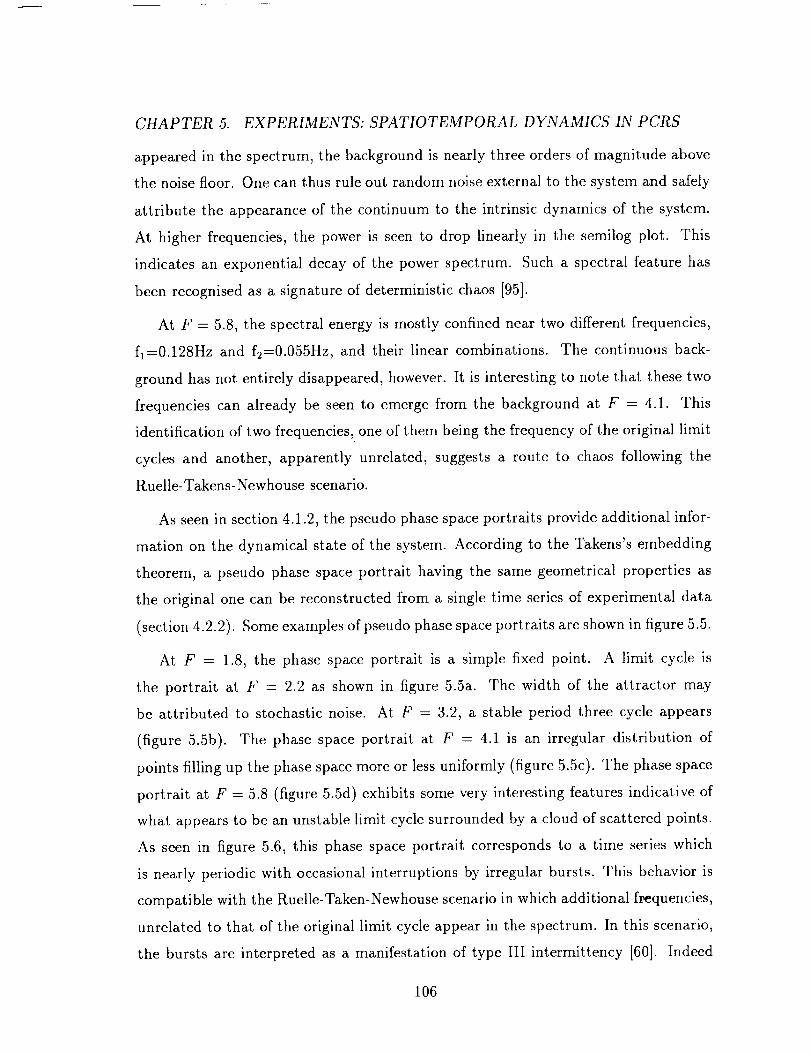
CHAPTER 5. EXPERIMENTS: SPATIOTEMPORAL DYNAMICS IN PCRS
appeared in the spectrum, the background is nearly three orders of magnitude above
the noise floor. One can thus rule out random noise external to the system and safely
attribute the appearance of the continuum to the intrinsic dynamics of the system.
At higher frequencies, the power is seen to drop linearly in the semilog plot. This
indicates an exponential decay of the power spectrum. Such a spectral feature has
been recognised as a signature of deterministic chaos [95].
At F = 5.8, the spectral energy is mostly confined near two different frequencies,
f1=0.128Hz and f2=0.055Hz, and their linear combinations. The continuous back-
ground has not entirely disappeared, however. It is interesting to note that these two
frequencies can already be seen to emerge from the background at F = 4.1. This
identification of two frequencies, one of them being the frequency of the original limit
cycles and another, apparently unrelated, suggests a route to chaos following the
Ruelle- Takens- Newhouse scenario.
As seen in section 4.1.2, the pseudo phase space portraits provide additional infor-
mation on the dynamical state of the system. According to the Takens's embedding
theorem, a pseudo phase space portrait having the same geometrical properties as
the original one can be reconstructed from a single time series of experimental data
(section 4.2.2). Some examples of pseudo phase space portraits are shown in figure 5.5.
At F = 1.8, the phase space portrait is a simple fixed point. A limit cycle is
the portrait at F = 2.2 as shown in figure 5.5a. The width of the attractor may
be attributed to stochastic noise. At F = 3.2, a stable period three cycle appears
(figure 5.5b). The phase space portrait at F = 4.1 is an irregular distribution of
points filling up the phase space more or less uniformly (figure 5.5c). The phase space
portrait at F = 5.8 (figure 5.5d) exhibits some very interesting features indicative of
what appears to be an unstable limit cycle surrounded by a cloud of scattered points.
As seen in figure 5.6, this phase space portrait corresponds to a time series which
is nearly periodic with occasional interruptions by irregular bursts. This behavior is
compatible with the Ruelle-Taken-Newhouse scenario in which additional frequencies,
unrelated to that of the original limit cycle appear in the spectrum. In this scenario,
the bursts are interpreted as a manifestation of type III intermittency [60]. Indeed
106
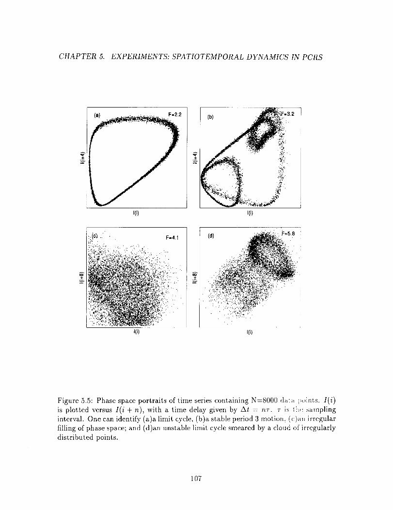
CHAPTER 5. EXPERIMENTS: SPATIOTEMPORAL DYNAMICS IN PCRS
l(i) l{i}
d ""'" v,::- J==58
.,/ ':-_.. .•.. •::"-__4r,',.¢
• -,_- ,¢_.__,:Z-:'".•.,.:_#_-'L-"_-'#3._,"-'.:_'-':.:",. i";'",_" _.". _ _," " ' :'_.':_,'_'_: ":'_i • ......._.:,...,_:_f:_>._.y:.,,,_.,,.: .
_"..i..._..." .r._,_ "..:.;:._.._:'.'.&_Z,,:,_. _... • "• .'.-' "-":'_':":;_- :',_:,_;._:'_"4: ."
• .'.'..._:."".:'.",'._L._t4t:_,__._-_....., ......=....,. ,'.,._;,,_,_!_. : '.'_., .."' "" "'z":;_,'."_._'B.t'.:. .......:, .,:..:;.¢.'.;_._.':....
"... ,_. _'j.i_,..
I(i} I(i)
Figure 5.5: Phase space portraits of time series containing N=8000 date_ ;,_,ints. I(i)
is plotted versus I(i + n), with a time delay given by At = hr. r is 1t::: sampling
interval. One can identify (a)a limit cycle, (b)a stable period 3 motion, (c)an irregular
filling of phase space; and (d)an unstable limit cycle smeared by a cloud of irregularly
distributed points.
107
CHAPTER 5. EXPERIMENTS: SPATIOTEMPORAL DYNAMICS IN PCRS
F=5.8
0 200 400 600 800 1000
'-1
v
-_ 1000 1200 1400 1600 1800 2000Q
t-
2000 2200 2400 2600 2800 3000
3000 3200 3400 3600 3800 4000Time (sec)
Figure 5.6: Time series of the local intensity for F = 5.8 showing a quasiperiodic
motion interrupted by intermittent bursts.
108

CHAPTER 5. EXPERIMENTS: SPATIOTEMPORAL DYNAMICS IN PCRS
some of the intermittent bursts appear to show an increase and then a sudden drop
of the amplitude of a subharmonic, which is a signature of type III intermittency.
5.3 Correlation dimension and Kolmogorov entropy
We have seen in section 4.1 that a number of quantitative methods have been es-
tablished for studing dynamical systems and distinguishing deterministic chaos from
random noise. In the following, we analyse quantitatively the nature of the chaotic
motion observed with a Fresnel number F = 4.1 by calculating the correlation dimen-
sion and the corresponding entropy, using the corresponding time series, a section of
which is shown in figure 5.3d.
The Grassberger-Procaccia algorithm was used to calculate the correlation di-
mension of the experimental chaotic time series [96]. This algorithm is based on the
Takens embedding theorem according to which N vectors )_(t,_) = [X(t,),X(t,_ +
At),... ,X(tn + (d- 1)At)] of length d ( the embedding dimension) can be extracted
from the time series and used to reconstruct the attractor in a pseudo d-dimensional
phase space. The delay At = iT, where T is the sampling interval, is chosen such that
the choice of T is made according to the remarks explained in section 4.2.2.
The correlation function or second order correlation integral is then calculated as
(see section 4.2):
1 N
C2( ,d) = zm.,), (5.2)m,r_l
d-1
where 0 is a step function and zm.,_ = __,lXn+i - Xm+il 2 is the Euclidean distancei=0
between the pair of vectors m, n and d is the embedding dimension. The correlation
integral thus measures the number of pairs of vectors with a distance smaller than _.
From equation 4.23, the correlation integral scales with the embedding dimension as
C2(c,d) o¢ e_exp(-d_-K2). (5.3)
For large enough d and small e, the correlation exponent u becomes the correlation
dimension D2. K2 is the second order Renyi entropy. These two quantities are lower
109
CHAPTER 5. EXPERIMENTS: SPATIOTEMPORAL DYNAMICS IN PCRS
bounds to the fractal (Hausdorff) dimension Do of the attractor and to the information
dimension D1 (Do >_ D1 >_ D2), and to the Kolmogorov entropy IQ (I(1 > K2),
respectively (see section 4.1).
Figure 5.7 shows log-log plots of the correlation integral for values of the embedding
dimension ranging from 7 to 27. The slope of the curves, which is the correlation
exponent according to eq. 5.2, appears to converge toward what is believed to be the
value of the correlation dimension D2. The local slope, calculated using a seven point
local average of the slope of the data of figure 5.7, is shown in figure 5.8 for different
values of d. Although the plateau, which should indicate the value of D2, is not very
broad, it does seem to converge, for d > 20, toward a value approximately equal to
5.2, as shown in figure 5.9.
According to eq. 5.3, a lower bound to the Kolmogorov entropy can also be ex-
tracted from the data of figure 5.7 by calculating the rate at which the correlation
integral drops with increasing values of the embedding dimension. In section 4.2.1
we discussed briefly that the Kolmogorov entropy measures the rate of information
flow in the dynamical system and is an indication of the system's sensitivity to initial
conditions. In an ordered system, it is expected to be zero, while in a stochastic
system, it should be infinite. For a deterministic chaos, its value would be finite and
positive. Figure 5.10 shows a plot of K2 versus d. Again, for d >_ 20, the entropy
appears to converge toward a value approximately equal to 0.16 s -1.
Although the relatively large value found for the correlation dimension may pos-
sibly put in doubt the validity of the algorithm used to calculate it, both the finite
positive lower bound to the Kolmogrov entropy and the non-integer value of the
correlation dimension seem to provide some evidence for the existence of a strange
attractor for the time series at F = 4.1.
110

CHAPTER 5. EXPERIMENTS: SPATIOTEMPORAL DYNAMICS IN PCRS
I I
09V
0V
1310
m
d=7
=27
Figure 5.7: Log-log plots of the correlation integral C2(_) versus distance _, with
increasing values of the embedding dimension d, for the chaotic output of Fig 5.7.
111

CHAPTER 5. EXPERIMENTS: SPATIOTEMPORAL DYNAMICS IN PCRS
10
8
6V
;>CD
2
I _ I I ' ' I T
• • • _ • I • _ ••
• • ..,: -.......::.
-. . .._.",__._1_:...-•" ".._z;,_'..-'_ " .. ".
.... ,,:_,-- ,, • ..
.........o : o""." • "i,_'__i,=27
d 7 "...__:
0-1.5 -1 -0.5 0 0.5 1
Figure 5.8: Local slope u(_) of the correlation integral of Fig 5.7. versus log e. The
slopes are averaged over 7 local points. The plateau indicates the range of linear
scaling for each d. The slope in the region of the plateau converges toward the
correlation dimension D2.
112
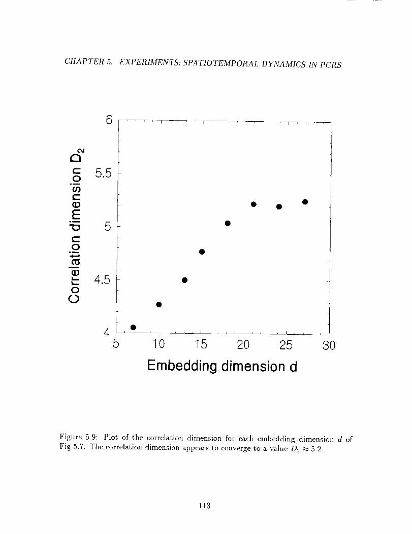
CHAPTER 5. EXPERIMENTS: SPATIOTEMPORAL DYNAMICS IN PCRS
Od
[21¢-O
Og1--Q
Eam
"O
e-O
im
,4...a
Q
oO
6
5.5
5
4.5
1 I ' F I
5 10 15 20 25 3O
Embedding dimension d
Figure 5.9: Plot of the correlation dimension for each embedding dimension d of
Fig 5.7. The correlation dimension appears to converge to a value D2 _ 5.2.
113
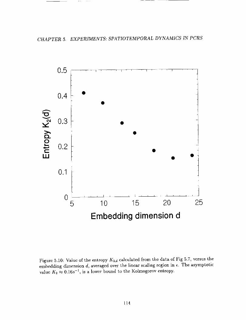
CHAPTER 5. EXPERIMENTS: SPATIOTEMPORAL DYNAMICS IN PCRS
.5 ' I ' _ I ' ' ' I
0.4
"0V
0.3
¢2.0b,--*-, 0.2e--
U3
0.1
_ _ _ , I k , , , i , , , t I , , k ,
5 10 15 20 25
Embedding dimension d
Figure 5.10: Value of the entropy K2,d calculated from the data of Fig 5.7, versus the
embedding dimension d, averaged over the linear scaling region in e. The asymptotic
value K2 _ 0.16s -1, is a lower bound to the Kolmogorov entropy.
114

CHAPTER 5. EXPERIMENTS: SPATIOTEMPORAL DYNAMICS IN PCRS
5.4 Wavefront dislocations
The transverse irradiance distribution within the aperture H1 as seen through
the PCM was recorded as a function of time. As the transverse confinement of the
system is relaxed, the distribution of structures across the PCR's beams becomes
more complex, containing more and more bright lobes and dark lines around them.
At the same time, the motion of the structures also increases in complexity, changing
from a simple periodic motion to an apparently chaotic dance.
Interferograms of the wavefront were recorded to reveal the presence of wavefront
dislocations or vortices [87] (also see section 4.4). In the interferograms, the defects
should appear as a discontinuity in the interference fringes and thus should be easily
identifiable. The number of defects and the complexity of their motions in time were
found to be strongly correlated to the temporal dynamics of the time series described
in section 5.2 as well as to the spatial decorrelation of the pattern. This suggests that
the topological defects may indeed act as the catalyst for the observed spatiotemporal
dynamics and induce the observed turbulence in a manner similar to that of the so-
called topological turbulence (see section 4.3.2). In this section, we will describe how
the transverse pattern changes when the Fresnel number, and thus the transverse
confinement of the cavity, is varied.
After a first bifurcation at 2 _< F _< 2.2, the transverse pattern varies in time
in a simple and periodic way. Some snapshots of the irradiance distribution, taken
at a half second interval between frames, are shown in figure 5.11. The irradiance
distribution is at first uniform, both in amplitude and phase. This lasts for about
eight seconds, after which time a folding of the phase appears at the center of the
pattern. This is manifested by a darkening of the area. Very rapidly, a pair of defects
of opposite charge develops from this fold at the center of the pattern. The two
defects split and repel each other, swiftly moving away along diametrically opposite
directions. They finally disappear at the boundary. The presence of the defects lasts
only about two seconds or so. The wavefront then quickly recovers and remains stable
for a period of time. Then, the sequence repeats itself. Figure 5.12 is an enlarged
115
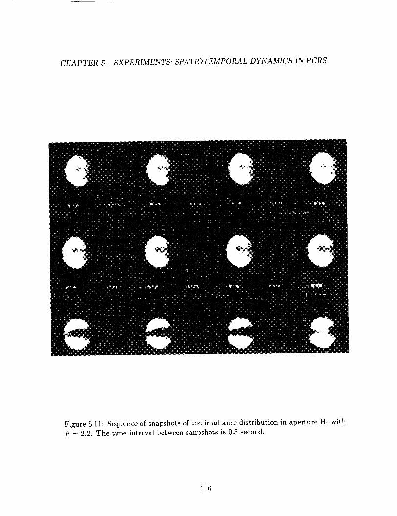
CHAPTER 5. EXPERIMENTS: SPATIOTEMPORAL DYNAMICS IN PCRS
Figure 5.11: Sequence of snapshots of the irradiance distribution in aperture H1 with
F = 2.2. The time interval between sanpshots is 0.5 second.
116
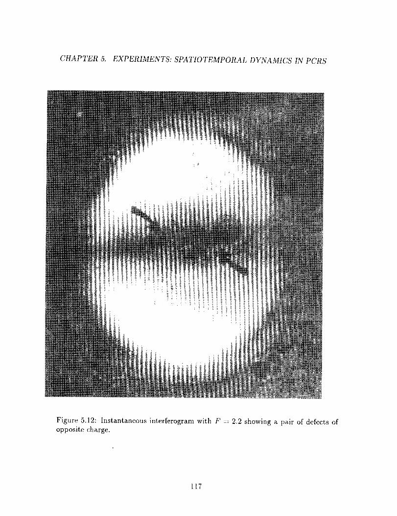
CHAPTER 5. EXPERIMENTS: SPATIOTEMPORAL DYNAMICS IN PCRS
Figure 5.12: Instantaneous interferogram with F = 2.2 showing a pair of defects of
opposite charge.
117
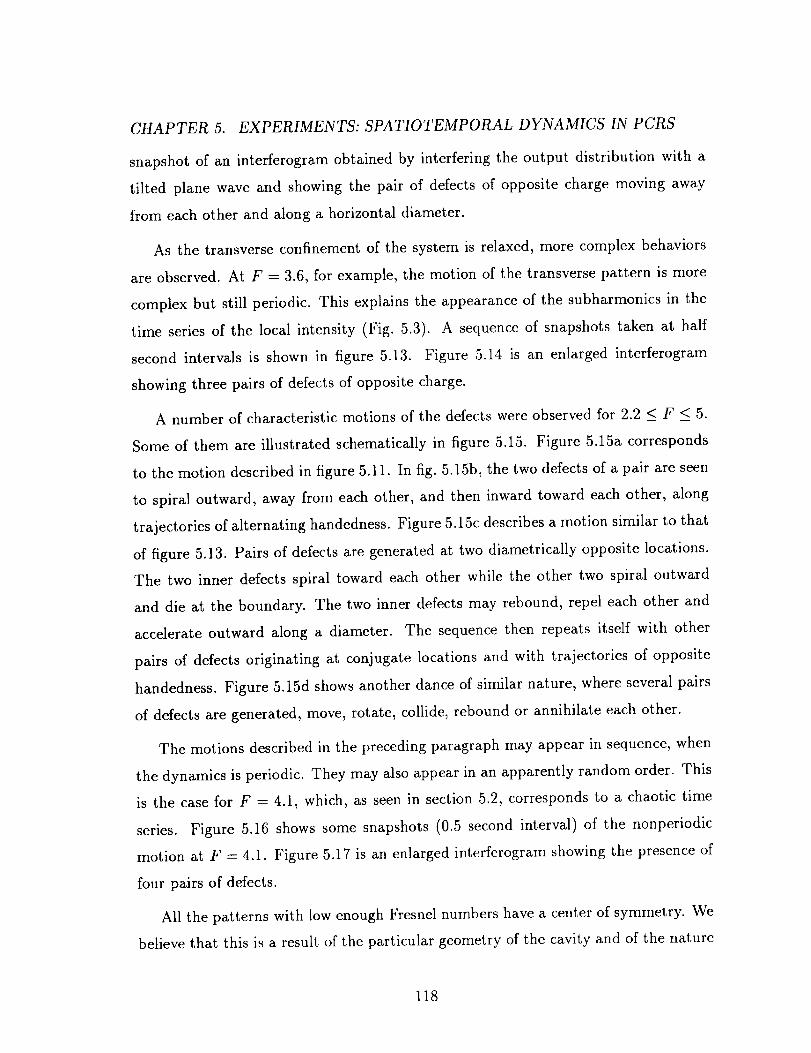
CHAPTER 5. EXPERIMENTS: SPATIOTEMPORAL DYNAMICS IN PCRS
snapshot of an interferogram obtained by interfering the output distribution with a
tilted plane wave and showing the pair of defects of opposite charge moving away
from each other and along a horizontal diameter.
As the transverse confinement of the system is relaxed, more complex behaviors
are observed. At F -- 3.6, for example, the motion of the transverse pattern is more
complex but still periodic. This explains the appearance of the subharmonics in the
time series of the local intensity (Fig. 5.3). A sequence of snapshots taken at half
second intervals is shown in figure 5.13. Figure 5.14 is an enlarged interferogram
showing three pairs of defects of opposite charge.
A number of characteristic motions of the defects were observed for 2.2 <__F < 5.
Some of them are illustrated schematically in figure 5.15. Figure 5.15a corresponds
to the motion described in figure 5.11. In fig. 5.15b, the two defects of at pair are seen
to spiral outward, away from each other, and then inward toward each other, along
trajectories of alternating handedness. Figure 5.15c describes a motion similar to that
of figure 5.13. Pairs of defects are generated at two diametrically opposite locations.
The two inner defects spiral toward each other while the other two spiral outward
and die at the boundary. The two inner defects may rebound, repel each other and
accelerate outward along a diameter. The sequence then repeats itself with other
pairs of defects originating at conjugate locations and with trajectories of opposite
handedness. Figure 5.15d shows another dance of similar nature, where several pairs
of defects are generated, move, rotate, collide, rebound or annihilate each other.
The motions described in the preceding paragraph may appear in sequence, when
the dynamics is periodic. They may also appear in an apparently random order. This
is the case for F = 4.1, which, as seen in section 5.2, corresponds to a chaotic time
series. Figure 5.16 shows some snapshots (0.5 second interval) of the nonperiodic
motion at F = 4.1. Figure 5.17 is an enlarged interferogram showing the presence of
four pairs of defects.
All the patterns with low enough Fresnel numbers have a center of symmetry. We
believe that this is a result of the particular geometry of the cavity and of the nature
118

CHAPTER 5. EXPERIMENTS: SPATIOTEMPORAL DYNAMICS IN PCRS
Figure 5.13: Sequence of snapshots with F = 3.6 (time interval = 0.5s) revealing amore complicated but still periodic motion.
119
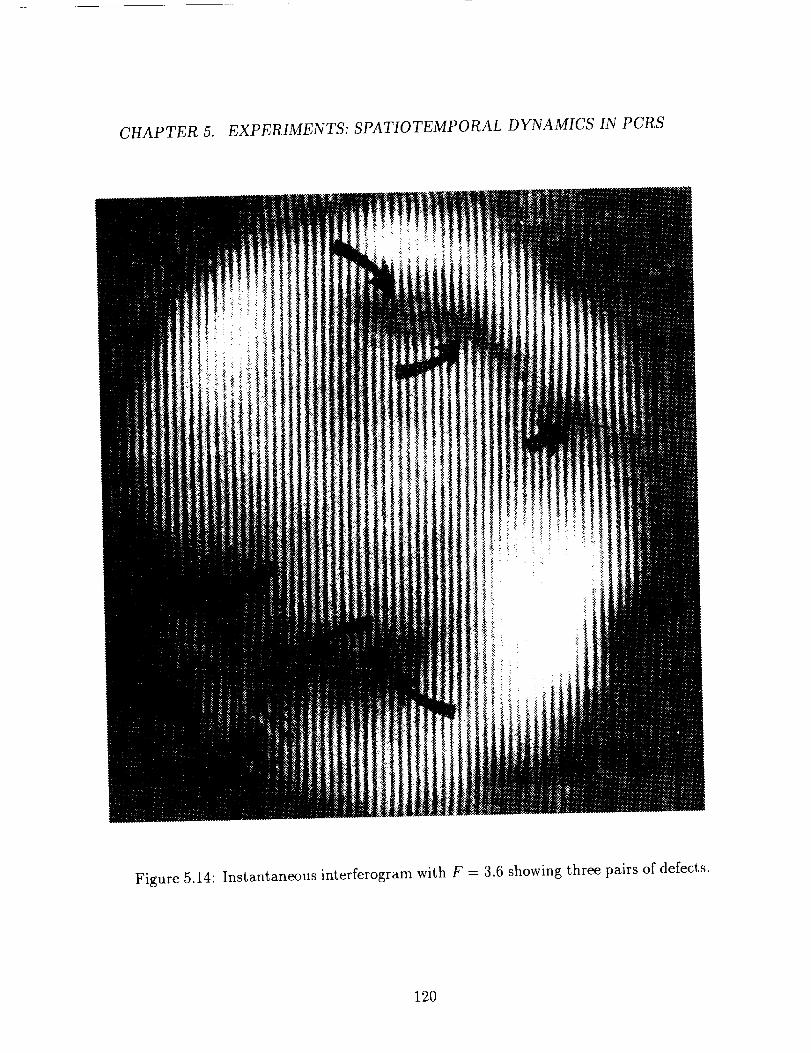
CHAPTER 5. EXPERIMENTS: SPATIOTEMPORAL DYNAMICS IN PCRS
Figure 5.14: Instantaneous interferogram with F = 3.6 showing three pairs of defects.
120

CHAPTER 5. EXPERIMENTS: SPATIOTEMPORAL DYNAMICS IN PCRS
(a)
(b)
(c)
(d)
Figure 5.15: Sketches of some typical motions of the defects observed with 2 < F < 5.See text for details.
121
CHAPTER 5. EXPERIMENTS: SPATIOTEMPORAL DYNAMICS IN PCRS
Figure 5.16: Sequence of snapshots with F = 4.1 (time interval =0.5s) revealing a
nonperiodic motion (horizontal scale compressed).
122

CHAPTER 5. EXPERIMENTS: SPATIOTEMPORAL DYNAMICS IN PCRS
Figure 5.17: Instantaneous interferogram with F = 4.1 showing four pairs of defects.
123
CHAPTER 5. EXPERIMENTS: SPATIOTEMPORAL DYNAMICS IN PCRS
of the PCM. Indeed, one round trip in the cavity involves two operations: phase
conjugation and imaging with unit magnification and inversion. Thus, if a certain
distribution f(r-") exists in the cavity, another f'(-r-') should also be present, at least
in steady state.
In the range 5 _< F _< 6, drastic changes in the dynamics of the local intensity
time series were observed. Similar changes are also found in the behavior of the
defects. At F = 5.8, for example, the spatial distribution shown in the sequence of
figure 5.18 is rather complex and indeed shows more structure than the pattern at
F = 4.1 (Fig. 5.17), which corresponds to a chaotic motion. However, not all the dark
lines in figure 5.18 contains true zeros. Thus, when F = 5.8, the number of defects
is actually smaller on average and the spatiotemporal complexity is lower than when
F = 4.1. The motion for interferograms at F = 5.8 is also simpler in appearance.
Figure 5.19 shows an instantaneous interferogram at F = 5.8, where only one pair
of defects is visible. When the transverse confinement is further relaxed, the motion
becomes chaotic again (Fig. 5.3f). Figure 5.20 shows an interferogram obtained with
a Fresnel number F = 8.6 and in which about eight pairs of defects are seen as they
execute a chaotic dance.
5.5 Defect-mediated turbulence
It appears, from the observations described in figures 5.11 to 5.20 and the corre-
sponding results of section 5.2, that the presence and the motion of singular points in
the wavefront ( the phase defects or vortices ), where both the real and the imaginary
parts of the field vanish and the phase is indeterminate (see section 4.4), may be
responsible for the loss of spatiotemporal coherence. According to the Coullet conjec-
ture, this in turn may induce turbulence in weakly coupled systems [79, 78, 80, 97].
In order to further illustrate the correlation between the number of defects and the
spatiotemporal dynamical behavior of the system, the following two measurements
were made.
The temporal evolution of the interferograms obtained with increasing Fresnel
124

CHAPTER 5. EXPERIMENTS: SPATIOTEMPORAL DYNAMICS IN PCRS
Figure 5.18: Sequence of snapshots with F = 5.8 (time interval = 0.5s) revealing a
more complicated pattern but executing a simpler motion
125
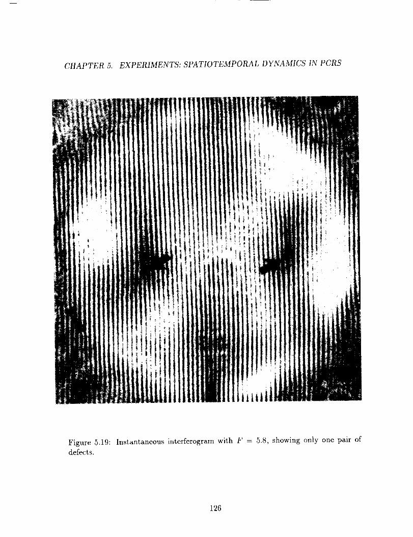
CHAPTER 5. EXPERIMENTS: SPATIOTEMPORAL DYNAMICS IN PCRS
Figure 5.19: Instantaneous interferogram with F = 5.8, showing only one pair of
defects.
126
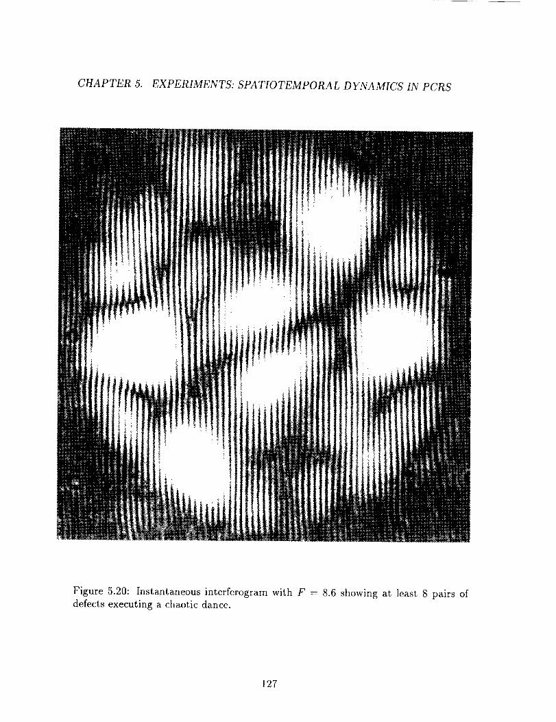
CHAPTER 5. EXPERIMENTS: SPATIOTEMPORAL DYNAMICS IN PCRS
Figure 5.20: Instantaneous interferogram with F = 8.6 showing at least 8 pairs of
defects executing a chaotic dance.
127
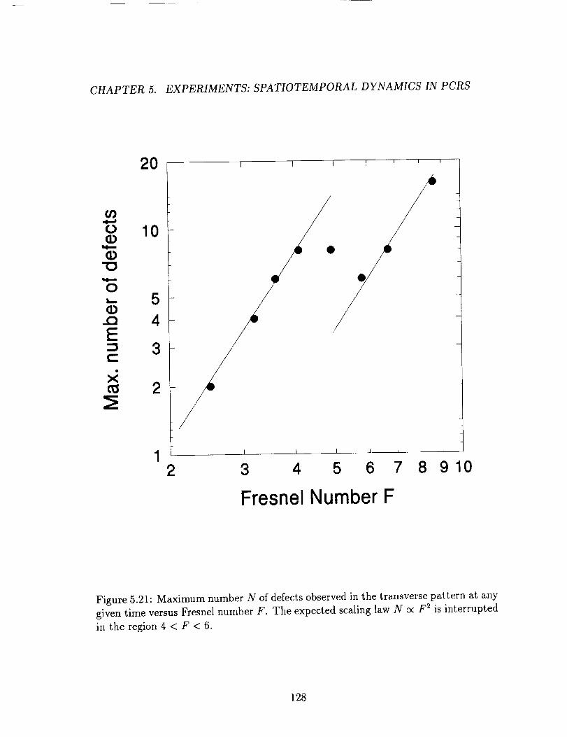
CHAPTER 5. EXPERIMENTS: SPATIOTEMPORAL DYNAMICS IN PCRS
2O
o 10
O
5
432
1 I I [ I J , ,
2 3 4 5 6 7 8910
Fresnel Number F
Figure 5.21: Maximum number N of defects observed in the transverse pattern at any
given time versus Fresnel number F. The expected scaling law N c¢ F 2 is interrupted
in the region 4 < F < 6.
128

CHAPTER 5. EXPERIMENTS: SPATIOTEMPORAL DYNAMICS IN PCRS
numbers were video recorded with a standard CCD camera and examined frame by
frame to determine the maximum number of defects appearing in the pattern at any
instant of time. The result is shown in figure 5.21. There are two regions, 2 _< F < 4
and F > 6, where the maximum number of defects appears to grow as the square of
the Fresnel number. This dependence is what is expected if, using simple diffraction
arguments, F 2 is interpreted as being a measure of the maximum number of speckles
( or of bright lobes ) within a cross section of the beam. The number of true zeros
between the bright speckles is expected to be of the same order as the number of
speckles, at least for large numbers [91, 87].
In addition, the temporal fluctuations of the local intensity were recorded at two
different locations in aperture H1, and a spatial correlation index [98] was calculated.
The spatial correlation function is defined as
with
N
_[i(7,,,_)- ,_(7,)][I(T5,,_+ r)- i(72)]c(_,, TS,r) = _='
s(_i)s(_i) , (5.4)
s(_) = [:(_J,,_)- i(_)] 2 , (5.5)
where 71, 72 are the two locations in the wavefront where the local intensity fluctua-
tions are measured, ](_'j) is the time averaged intensity at _, n and F are the running
time and time delay, respectively, measured in units of the sampling interval r.
In the experiments, the local intensity fluctuations were measured at two points
only, distant by approximately one half the diameter of aperture HI. A spatial cor-
relation index can then be defined as
K(1¢1 - 7_1)= MaxC(¢i, 72,r), Yr. (5.6)
The correlation index runs from 0 to 1. It is high when the fluctuations at 71 and
72 are highly correlated. It is equal to one when the fluctuations at 71 and 72 differ
only by a time delay, as one would expect if a transverse wave sweeps through the
pattern. It drops to small values as the fluctuations at 71 and 72 become decorrelated.
129

CHAPTER 5. EXPERIMENTS: SPATIOTEMPORAL DYNAMICS IN PCRS
_:0.8
.i
c-O
00w
o_
Q.
0.2
I i q
@-----@_
I I I I , i , ,
2 3 4 5 6 7 8910
Fresnel number F
Figure 5.22: Spatial correlation index versus Fresnel number F. Comparison with
Fig. 5.21 reveals the relationship between the spatial correlation and the number of
defects.
130
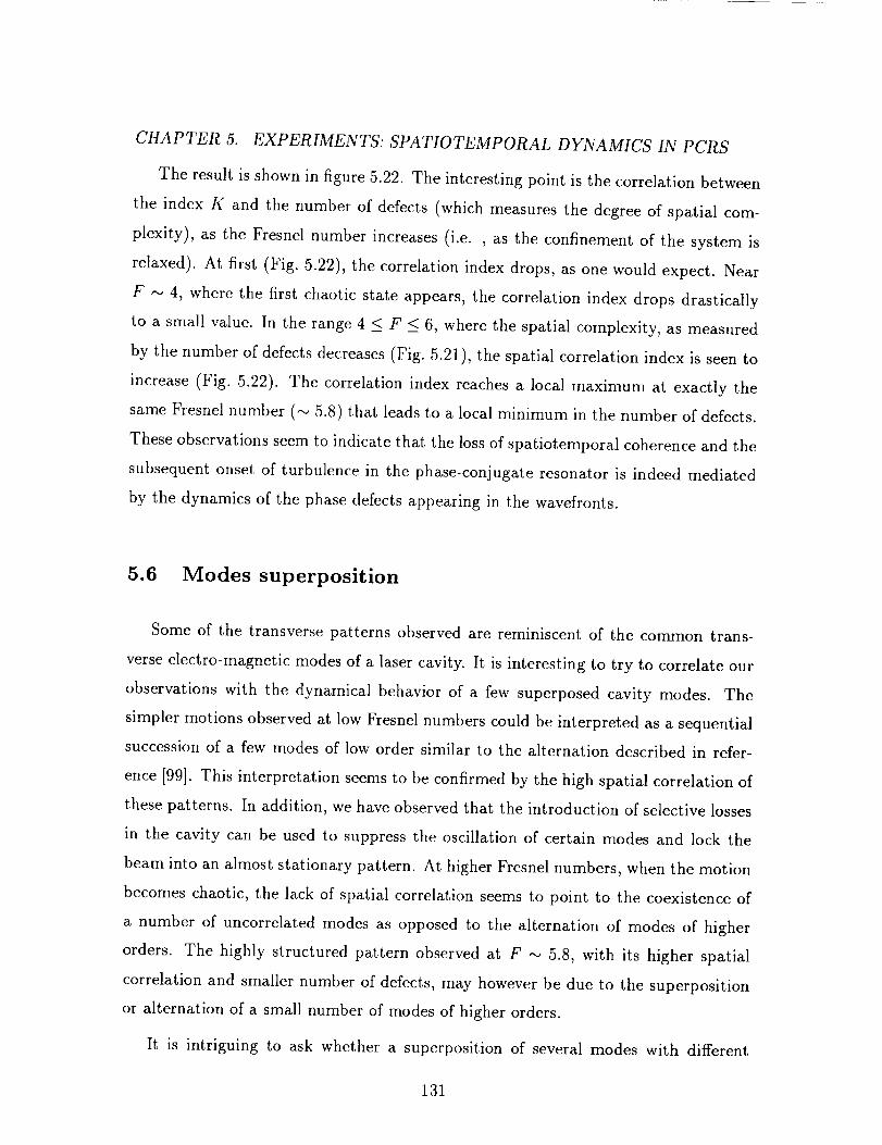
CHAPTER 5. EXPERIMENTS: SPATIOTEMPORAL DYNAMICS IN PCRS
The result is shown in figure 5.22. The interesting point is the correlation between
the index K and the number of defects (which measures the degree of spatial com-
plexity), as the Fresnel number increases (i.e. , as the confinement of the system is
relaxed). At first (Fig. 5.22), the correlation index drops, as one would expect. Near
F -,_ 4, where the first chaotic state appears, the correlation index drops drastically
to a small value. In the range 4 < F _< 6, where the spatial complexity, as measured
by the number of defects decreases (Fig. 5.21), the spatial correlation index is seen to
increase (Fig. 5.22). The correlation index reaches a local maximum at exactly the
same Fresnel number (_,- 5.8) that leads to a local minimum in the number of defects.
These observations seem to indicate that the loss of spatiotemporal coherence and the
subsequent onset of turbulence in the phase-conjugate resonator is indeed mediated
by the dynamics of the phase defects appearing in the wavefronts.
5.6 Modes superposition
Some of the transverse patterns observed are reminiscent of the common trans-
verse electro-magnetic modes of a laser cavity. It is interesting to try to correlate our
observations with the dynamical behavior of a few superposed cavity modes. The
simpler motions observed at low Fresnel numbers could be interpreted as a sequential
succession of a few modes of low order similar to the alternation described in refer-
ence [99]. This interpretation seems to be confirmed by the high spatial correlation of
these patterns. In addition, we have observed that the introduction of selective losses
in the cavity can be used to suppress the oscillation of certain modes and lock the
beam into an almost stationary pattern. At higher Fresnel numbers, when the motion
becomes chaotic, the lack of spatial correlation seems to point to the coexistence of
a number of uncorrelated modes as opposed to the alternation of modes of higher
orders. The highly structured pattern observed at F ,-, 5.8, with its higher spatial
correlation and smaller number of defects, may however be due to the superposition
or alternation of a small number of modes of higher orders.
It is intriguing to ask whether a superposition of several modes with different
131

CHAPTER 5. EXPERIMENTS: SPATIOTEMPORAL DYNAMICS IN PCRS
frequencies could produce patterns in which the defects would move around in a
manner similar to the motions described in section 5.4.
As an illustrative example we used a superposition of three Gauss-Hermite modes
of the form
Em,_(x,y;t) = Am_Vm g,, exp i(hm,_t + ¢m_) w% j,
where the Uj's are Hermite polynomials, w is the beam "waist", ¢m,_ = (m + n + 1)7/
and rI = _'/3 (arbitrary choice), 5m,_ is the frequency detuning and A,,_ is the weight
of mode mn [94].
We chose the three modes TEM 01, 10, and 20 with respective weights 1, 1, 1/3
and respective detuning 1/2, 1, (Vr5 + 1)/2. A sequence showing the evolution of the
pattern in time is shown in figure 5.23. The shaded regions are the bright spots and
a and b indicate the position of the roots of Re(E)=Im(E)=0, where the defects
are located. The arrows show the directions of their motions. Figure 5.24a shows the
motion of the two conjugate defects projected on a plane. Starting at point A for
defect a (solid dots) and B for defect b (empty squares), the following motions are
observed. At first, defect a rotates slowly counterclockwise near the center the field,
while defect b accelerates upward, disappears at the upper right, reappears at the
upper left corner and swiftly moves down across the field. This motion is labeled 1 in
Fig. 5.24a. Next (motion labeled 2), defect a , still moving slowly, changes direction
and starts upward while defect b disappears at the bottom left and reappears at the
bottom right. Defect a then accelerates out at the top left, reappears at the top right
and rapidly crosses the field toward the bottom left, while defect b starts executing a
slow clockwise rotation near the center of the field. In a certain sense, the two defects
have exchanged their roles but with antisymmetrical motions. This type of motion
continues, leading to the path diagram shown in figure 5.24b.
Another interesting illustration given here is a scalar wave _b(r, t) combining the
three modes TEM 00, 01 and 20 with fixed relative phases. For example, ¢ =
al(t)U2o + a2(t)Uoo + iaa(t)Um, where ai(t)'s are real functions of time. This ex-
ample shows two opposite charge defects moving apart along the x-axis as seen in
132
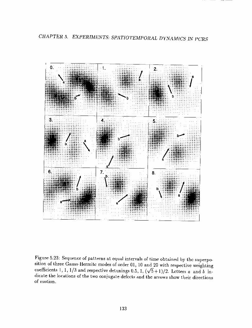
CHAPTER 5. EXPERIMENTS: SPATIOTEMPORAL DYNAMICS IN PCRS
o. :iiiiiiiiiiiiiii ::: i :iiiiiiii i::, • 2............ , ...................... ::,,: ....................__.......... • " / .............. o.*ioo ............ "lllllmlnlUlll, ......... ,lilllll .................. ,lllmlll.
.......... :|:==|::::::: ............. : .......................................... _ ..... ,,II,,,,,,, ....... :::. ::::.lllll::::z:: ........................"" ..... _..,oummilllnll lllla.,,, ........ Onlllllln* _ "''''''' .... ,_lllllln.,..]• ,,,I ..... "IIlIIIN Illl.lllll ii I ........ llllll ..... Illllllll.-......... a.... ,,,,,,Ill% ............... _ .................................. I,,ii, ......... ,=mnmlnll I=,-.., ....... ::,;;_;:::::::: ..... ==== ......... =nil ......................... ii_ii. .................. "''_e]_!] ..... 4 ........... _ ,lnllllilllllmlll ,in • II .......... ,11 iiiii .... "lllil. .
l=,, liD Illllillll, ..... l,llle .... ii I ''iliUllOilmllllellO, in I in 1''' in ill .... ,nell .....
• i I • iiiniill ................ l "• __,. l, ............. ,o,,,o |i
inDia llnlllill,. ..llmlimilll i ' Ill ...... ill ...........l..-,,i,,,, ...... _,, ....... ,..lllll:.'" _,,.: ............... ,_,_Ill,... , .................:r!L.-..HHii|!i:b========================7b .......... ::::ii i ..... ollgi** o lllilll .............. ilnlllilll . .._:.."llllllllllllllll ........ iii1.11111111111 I .............. IIIIIIIIII .............IIIllllllllllllll .............. illllllll .....
;::::_:,, .======================================= ========================================
i i!!!2!!!i2:: i24 2i 2. : 52 iiii2i!2ii ......:::::::::::::::::::::::::: ::::::::_::::.: ;::: .............................. .::............................................. :;:::;:;: ::::::: ..................
............................... == ........................... :::::::::: :;;::;:::" ::: ......................•.=:::: .................. • ......
• ,mllimai,:::. '::.:::::::::::: ,l=mam, :::. ........IIIlllllll
!E|i!|!i,mll I,.: /:::::: :o _ll_" .... " .................. ,,,,,,,::::::::..:: ::::::II il ill . -- '_ '''11_111 ..... I,, ........... Illllllll ................ ,I
,=m! =,,:. b:::::::::_ :: :::::::::: ::::::::::::::::::::::::::::: : ............. :::.,,,|=,,::...:::,,::: ........ : ........... ===........................ • ........................... i!_ ............ ::liE= ............... _',-,=,, ...........:::::::::::::::::: ....................... iiiii: .... ::::::: /:::::l|l:=::::::..... ' .... _.llllllllll ......... /_:llllllllll................... :::: ............ =IIII ................. ,II, ...........
,,,1==. ............ /,Olililll* ...... _ .lllll*.
6_iiiiiiii]iiiiii: 7. ............. 8. " ............
.... IIIIIIIIIIIIll.> _ .......... ib .lllllllll. I ...........
.... Illllllllllll ...... / _ im ........ ,=ll ill, ................ • llllll ........... • •''''lllllllllllll, ......... • in Ill • ..................... ==muunmm,..n ....... ...... l ..,11"" lllll,-..... ........... "" I" 111 ..... _ .........
,-lniummmll IIm, ....... ,, ....... ,nni---mn::i • :: ........ nmmmmnl ................... lllllll l ........... :l .... ,,II,. ' ......... _" .... :[ .........
immmiimm illh __ ..... ilWWl .... "lliill* .... i/i liilll,I IIII I" '1111111 .... IIIIII I I
I ...11 i,. .*1 I iii . . b ''1111111" .... IIIIIIi Illlllllllllllll_,..V.illllllll ::::::1111 ......... III ...... III ........ IIIIIII
..................... ;n_ -_::::::::::_:_ ......... ,m mn.............. :_um mm_
...................... i .... i,, ._ • in_ ....... _ ......... _ .... _U II'
iiiiiF! i!!,!':::::::. a :::::::: : :;:::;:;:::::;:;:;:::
::::,_:,, "'::: ............................................... iiiiiiiii .
Figure 5.23: Sequence of patterns at equal interva]s of time obtained by the superpo-
sition of three Gauss-Hermite modes of order 01, l0 and 20 with respective weighting
coefficients 1, 1, 1/3 and respective detunings 0.5, 1, (v/-5+ 1)/2. Letters a and b in-
dicate the locations of the two conjugate defects and the arrows show their directionsof motion.
133
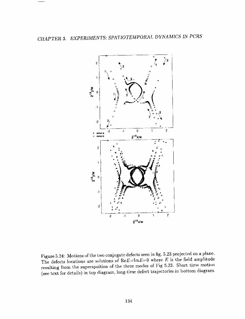
CHAPTER 5. EXPERIMENTS: SPATIOTEMPORAL DYNAMICS IN PCRS
_o
-2
o o
\3 o_ _3
1_o o• g
oo: A_.. oo_...o
oo ° o •
o [] •
i
-2 -1 0 1 2
2_/2x/wi
o
o
• defect •
o defect b
_0OJ
-2
oEB
dP _ 0 0
°.-.5o _o.
",1."'g'_" o_•"2__ .9 _ o
• _,r D ,p •o •o
o o o oio
, , l , .o. L .... i .... J , • , ' •
-2 -1 0 1 2
2_/2X/W
Figure 5.24: Motions of the two conjugate defects seen in fig. 5.23 projected on a plane.The defects locations are solutions of ReE=ImE=0 where E is the field amplitude
resulting from the superspoition of the three modes of Fig 5.23. Short time motion
(see text for details) in top diagram, long-time defect trajectories in bottom diagram.
134
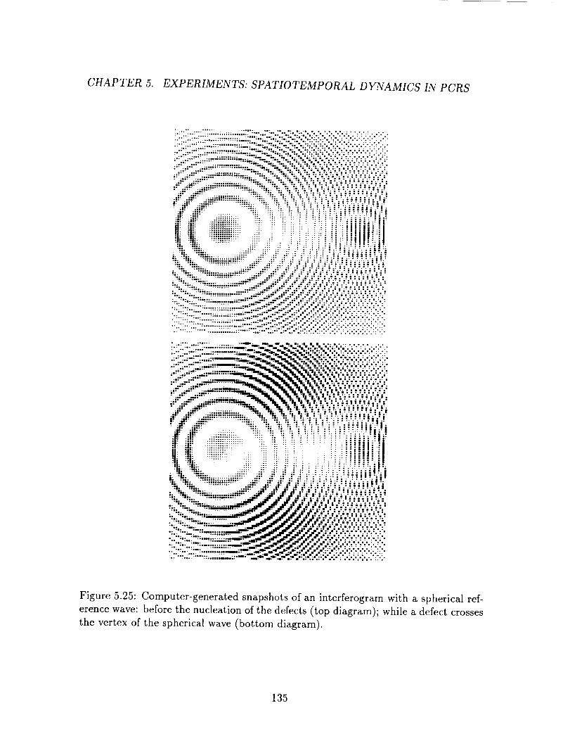
CHAPTER 5. EXPERIMENTS: SPATIOTEMPORAL DYNAMICS IN PCRS
i!j!i!j! i!ij !i i !i" 4" .-iii!.='-'"":"""!ii.;._;.;.%. ..'i. .:L"C.;. ".';"- -:-"".': ":"".; "=.-:! (:' f4"_ ;i":;" '_:::._::'!:: : " .:.:_:_!-''iiiiji_'a.
illill:iijiiji!!iiiiili!:i:ii i :)iiii:jjiijji: ij
i
:.:-:':;.,..:':::;...;=:::,,;,..--_..,:,_-_,-'-,r._.',;:,,.',,,,...,-.-.:..:..... . ; ...- ;
•:".:..":......:'---,_._'.-:'._.__-:'..'.:.:,,'.:-v-','.:.:.:.:,'.'.; ,"..... • . " ..,,,.*Mim,_* ." " '" _1,,,_"_'_"_"°& %'' _' %"*="*"*" : '"....:_.. ...-...-,..,..,..........:.
• i:" .i:=* .,,,,i_**_*'" '. '
..:_%, [ =.%*;,; .';*.'.." ,:.-..• ***;:* .i:_ "_," " " • - _ i :,'** *,'=i=-" *= *..* : **':',*" :';
i", .,,'" .... -,_..-=_;=""'_T'". "" . " " "li'"1% -= ".'i _ I .= .= ; ." ,','. •"
.if" .*:._." ....ii_;_l; ...**. ""._. "_1_I1___."'._.'IIL_ '_." "_ I "!-'!. ili**_ _ I ".'-'i' : I -* ." -*.... : ............. ,__ .___,_,, ,.,...... :........,...._.it.._:_.,,: ...... _'.'_,'_I_._ "i, "=i.'li I. ;.{._.'..=.'i'"i._ii i'-".; ._'ii;" "-''" "";'_:;::':L_:;_. ""_.S:"!i. "!i ;i I. -' "-"". ; ";: : • = ; i .'." ; I ."
o , ii o . .allmllilliillolll. I i . l .I i* I • i i m i I I i i i I i
;i;."_ .-i"'_ ...... "'!ii; '!i. '!i. "i."iTT "-_":i i ! !" ! ! i i: ! i
Ili_ !!i ii _: : : _ i_ !_::: : ii !!iiiil :il_i _'!i :T...... : "! ii ::i !:: '. i i i.'ii!-"';l'.',:il
i."'5=.""ii,--,........._;i_!:;i!,.iF.i!i!.i"-!;!;"-L!i'.!!iiiii.;"i!.'. " " "*=|'"" ...... ;":*';' .:.*? .-': ,**: :* -*' ..* ,* .: .! " ,.* : i .',*,'.', " ..
'.":!.li-i':"ii_i-..l,1='ii_i_'".4iP..jir iJ_.i"i!'.i"I"J','."i"i_'.'.""ll.:.'-"_l
,.,.':.,:,._"_.._._,,_.,_j._.¢,,_...-.,'-,.,'." v v-" ".,">._..:"-,,:::::__(,:',"-'.'::,,',',',',"::'.,_.j,.____2;"" "°:••" "_;'*:--° ...... '_' " ',_I " ' "'-*'n.l*-'!.;* i * ='" = i,; %%................... 3--.__.,.-.._.. ............ ....•,....,..,............. .,,,.:;:,.....•.....,,: .... ......... e_--. _T-_F_._.._;.,_., _ ;,,, .,,,,.,.,.,.,,. • %......... _ ..... :_,. ;P_, ...........
........ • nl.•.°** °. .u. m m, _or °o _ • n-* ° . i • .........:.. ":... ""':. ........ .:'--".--" ,._',.'::'%':::'.'.":;.".':":V;';';';';;.L:-:;
Figure 5.25: Computer-generated snapshots of an interferogram with a spherical ref-
erence wave: before the nucleation of the defects (top diagram); while a defect crosses
the vertex of the spherical wave (bottom diagram).
135
CHAPTER 5. EXPERIMENTS: SPATIOTEMPORAL DYNAMICS IN PCRS
experiments with a Fresnel number F = 2.2 (figure 5.11). Figure 5.25 shows a com-
puter generated interferogram of the wavefront with a spherical wave. Figure 5.25a
shows the interferogram of the uniform wavefront with no defect. It displays typical
Newton's rings. A short while later, two defects appear at the center and move apart
along the x-axis. Figure 5.25b shows the interferogram of the wavefront at the time
when one of the defects crosses the reference spherical wave. The spiral fringes reveal
the spiral nature of the wavefront. As the defect disappears at the boundary, the com-
plete rings are recovered again. A similar behavior was observed in the experimental
recordings for F = 2.2. Figure 5.26 shows snapshots of interferograms obtained by in-
terfering the cavity beam with a spherical reference beam from the same laser. When
one of the defects passes through the vertex of the spherical reference wave, it creates
spiral fringes.
These examples are presented for illustrative purposes only. They show that the
superposition of a few low order modes, with appropriate weights and detunings, can
produce a great variety of patterns and defect motions, some of them resembling
qualitatively what is being seen in the experiments, but they do not prove that this
is the correct representation. We will explore this modal superposition approach to
represent the spatiotemporal dynamics in a PCR in the next chapter.
5.7 Discussion and conclusion
As mentioned in chapter 1, phase conjugation via four-wave mixing in BaTiOa is
known to be itself unstable in some regions of parameter space, leading to a pulsating
or chaotic phase-conjugate beam [22, 27]. These instabilities appear to be related
to the existence and competition of several gratings in the crystal. In addition, self-
phase-conjugation of pump two, which is readily observed in BaTiO3 , produces a
feedback to the laser which can also cause instabilities. Two different tests were
made that lead us to believe that these two factors did not play a major role in the
experiments.
Four-wave mixing without the cavity (mirror M removed) and with an external
136

CHAPTER 5. EXPERIMENTS: SPATIOTEMPORAL DYNAMICS IN PCRS
Figure 5.26: Experimental snapshots of the interferograms of wavefront containing a
pair of defects with a spherical reference wave: before the nucleation of the defects (top
diagram); while a defect crosses the vertex of the spherical reference wave (bottom
diagram).
137
CHAPTER 5. EXPERIMENTS: SPATIOTEMPORAL DYNAMICS IN PCRS
probe beam was tested for parameter values comparable to these used in the exper-
iments. In all cases, the phase-conjugate beam was found to be quite stable. This
appears to indicate that the observed dynamics is that of the phase-conjugate res-
onator, which of course involves a possibly complicated nonlinear interaction with
feedback between the resonator and the photorefractive crystal, rather than that of
the four-wave mixing process. Furthermore, PC instabilities often require a rather
high coupling constant (3'I _ 6 in Ref [22]). In our crystal, the coupling constant was
estimated to be between 2 and 3 only (see chapter 3).
Tests were also made to detect the presence of self-pumping. With pump two alone
incident on the crystal, strong self-phase-conjugation was observed. The presence of
self-pumping is easily revealed by the usual beam fanning and internal reflections
in the crystal. The feedback of the self-conjugated pump beam into the laser did
cause some instability of its output. However, as soon as pump one was turned
on, the fanning died out, the path of pump two straightened out inside the crystal
and the self-conjugated beam intensity dropped to negligible values. Apparently, the
presence of pump one did effectively erase all the extraneous gratings responsible for
self-pumping. The same transverse patterns and dynamical behavior were observed,
confirming that feedback due to self-pumping was negligible in our experiments and
was not influential in our data.
In summary we have studied some aspects of the spatiotemporal dynamics of a
phase-conjugate resonator. The control parameter was the resonator Fresnel number.
Time series of the local intensity fluctuations were recorded and analysed by means
of spectral analysis and embedded phase space portraits. A number of occurrences
characteristic of low dimensional dynamical systems were observed, i.e. in order of
increasing control parameter: a bifurcation from a stationary to a periodic state,
followed by more subharmonic bifurcations; the occurrence of a chaotic state char-
acterized by the appearance of a continuous background in the power spectrum; the
appearance of an additional frequency unrelated to the fundamental frequency of the
periodic motion; the occurrence of intermittency; and the final development of what
appears to be a fully turbulent state.
138
CHAPTER 5. EXPERIMENTS: SPATIOTEMPORAL DYNAMICS IN PCRS
The occurrences of these events were found to be quite reproducible, providing
some evidence for the presence of a deterministic chaotic state of the cavity field.
Further evidence is given by calculating the correlation exponent and the Kolmogorov
entropy at a Fresnel number leading to a chaotic time series.
The spatial complexity of the pattern was studied by video recording and by
interferometry, revealing the leading role played by the wavefront dislocations or vor-
tices. The number of phase defects and the spatial correlation index of the wavefront
were observed to follow similar trends as the transverse confinement of the system
was relaxed. This suggests that the spatiotemporal chaos of the cavity field may be
mediated by the phase defects.
139
Chapter 6
A model of spatiotemporal
dynamics in PCRs
6.1 Introduction
In this chapter we present a truncated modal expansion approach to model the
spatiotemporal dynamics of a PCR. Nonlinear dynamical problems that include the
transverse dimensions and are described by systems of partial differential equations
(PDEs) remain a theoretical challenge and do not benefit from well established
experimental methodologies [100] as do systems of ordinary differential equations
(ODE) [60, 101]. Furthermore, their numerical analyses require large computational
budgets [56, 102]. We will test a relatively simple mathematical scheme to represent
the transverse dynamics of the PCR without requiring prohibitive computational
budgets.
This chapter has two aims. The first is to describe and establish the soundness
of a somewhat arbitrary yet sensible modal decomposition approach to study the dy-
namics of PCRs with modest Fresnel numbers. This is done by comparing numerical
results with actual experimental data. The hope is that this comparison, although
complicated by the difficulty in measuring experimental control parameters exactly
140

CHAPTER 6. A MODEL OF SPATIOTEMPORAL DYNAMICS IN PCRS
and by the problematic effect of stochastic noise, will prove sufficiently convincing to
confirm the usefulness of the approach. The second is to illustrate the relationship
existing between the dynamics of the optical vortices observed in PCRs [87, 88, 86]
and the spatial correlation of the oscillating beam.
The chapter is organized as follows: The PCR's equations and boundary con-
ditions within approximations compatible with experimental conditions are stated
in section 6.2.1. Arguments justifying the modal expansion approach are given in
section 6.2.2 and the method is then used to arrive at a set of modal amplitude equa-
tions. In section 6.3, a particular set of parameter values is chosen and the system
is integrated, using the off-Bragg detuning as a control parameter. Different dynam-
ical behaviors are identified from local time series, power spectra and phase space
portraits. Examples of vortices' motions and spatial correlation maps are given in
section 6.3. Experimental results are presented and discussed in section 6.4 and a
summary is given in section 6.5.
6.2 The modal expansion model
6.2.1 Phase-conjugate resonator
The PCR is sketched in fig. 6.1. Its active element is an externally pumped
photorefractive medium acting as a PCM. Maxwell's equations for the optical field in
the medium lead to the following coupled equations (see Appendix A):
2k +]c''v+_+_ Al(x,y,z,t)=-Q(z,y,z,t)A4(x,y,z,t)e ibz, (6.1)
- 2---k--+_:2"V+c_+_-_ A2'(x,Y;'_,t)=Q(x,Y,z,t)m3[x,y;t,t), (6.2)
2k + ]ca. V + _ + _ ma(x,y,z,t) = -Q(x,y,z,t)A2(x,y,z,t), (6.3)
( iV_ O)- 2----_--+]¢4.V+a+70- 7 A4'(x,y;,_,t)=Q(x,y,z,t)Al.(x,y;:_,t) e ibz, (6.4)
141

CHAPTER 6. A MODEL OF SPATIOTEMPORAL DYNAMICS IN PCRS
mirror M lens L
Figure 6.1: Four-wave mixing in a photorefractive phase-conjugate resonator (PCR):
A1, A2 are two gaussian pump beams; A3, A4 are the left-going and the right-goingbeams inside the PCR; mirror M allows feedback of field back into the phase-conjugate
mirror (PCM); apertures H1 ,H2 confine the transverse dimensions of the propagating
beams.
142

CHAPTER 6. A MODEL OF SPATIOTEMPORAL DYNAMICS IN PCRS
where, in spirit of the slowly varying envelope approximation, the field in the medium
is written as4
E(x,y,z,t) = + c.c., (6.5)i=l
v = c/fi is the speed of light in the medium, fi is the average refractive index. ]¢j are
unit vectors pointing in the direction of the four wavevectors in the medium. The
wavenumber is kj = _o/v, where w is the angular frequency of the pump and o_ is the
linear absorption coefficient. VT is the transverse gradient operator. The parameter
b is the wavevector mismatch (momentum mismatch along the z-axis) measuring
the departure from the Bragg condition. This off-Bragg parameter is introduced as
a means of varying the amount of phase transfer between the waves mixed in the
nonlinear medium and is later taken as the control parameter.
The equation for the phase grating Q is derived from the standard band trans-
port model of Kukhtarev [103] and reads, in the single grating approximation (see
Appendix B),
OQ(x,y,z,t)
r, Ot + CQ(x,y,z,t)= (6.6)
%C ( Al(x'y'z't)A_(x'y'z't)eib_ + A_(x,y,z,t)Aa(x,y,z,t))Io(z,v,z,t)
where C = [Eo + i(Eq + ED)]/[Eo + i(EM + ED)].
The boundary conditions for the wave equation in the medium are determined by
the cavity geometry. The transverse confinement of the cavity is controlled by two
square apertures H1 and H2 of sides 2avcm and 2am respectively. The first aperture is
located near the phase-conjugate mirror in the front focal plane of the lens (fig. 6.1).
The second one is in the back focal plane of the lens next to the planar mirror. The
transverse confinement is measured by the cavity Fresnel number defined as
F = 4amapcm/)ff, (6.7)
where A is the wavelength in vacuum and f the focal length of the lens.
One cavity round trip, starting at the PCM, consists of a truncation by H1 and
imaging in a 4-f afocal system with a pupil H2. Thus, the amplitude A4 is proportional
143
CHAPTER 6. A MODEL OF SPATIOTEMPORAL DYNAMICS IN PCRS
to the truncated convolution of A3 with a point-spread-function which is the fourier
transform of the aperture H2. According to Fourier optics [104], the field at the plane
of the mirror M, £(x,y,-L+,t), is proportional to the convolution of the Fourier
transform of the field Aa(x, y,0 +, t) at the exit plane of the crystal and the Fourier
transform of the square aperture H1, i.e.
L)- eik°L 2a_cm ]£(x'y'-L+'t+--c i_f F{A3(x'y'O+'t)}*F{rect( X_)rect(2apcm )} , (6.8)
where feet(x/2) =1 for -1 < x < 1 and = 0 otherwise. The field is then mirror
reflected and truncated by the aperture H2 such that
L L -x -y
g(x,y,-L*,t + c): rE(-x,-y,-L*,t + c) • rect(2_-m)rect(2--_-m),(6.9)
where r is mirror M's reflectance coefficient.
The field ,f.(r, y, 0-, t + _-) is a multiplicative of the inverse Fourier transform of
£(x,y,-L +,t + £), i.e.c
E(_,y,o-,t + 2L)C
_ eikOLF_l{g(x,y_L+ t + L)} (6.10)jAf c
ei2koL= a_f_ A3(-x'-Y' °+' t) rect(2apcm--x)rect(2apcm-y )]J
* [4a_sinc(2amx)sinc(2amy)],
where sinc(x) -- sin(Trx)/(Trx).
Thus, we can write the input field A4(x,y, 0 +, t) in terms of the outgoing phase
conjugate beam Aa(x, y, 0 +, t) in the following way:
2L ei2k°L II//+a"_" 0 + t)sinc [2am(x' + x)](6.11)A4(x,y,O+,t +--) = -4a_r A3(x',y', ,C _---_JJ--apcm L Af J
sine "2am(y' + y) dx'dy',Af
144
CHAPTER 6. A MODEL OF SPATIOTEMPORAL DYNAMICS IN PCRS
Using the resonator Fresnel number F = 4amavcm/A f and normalizing the trans-
verse coordinates to the aperture size avcm, we find
+ 2L) = _r(F/2)2ei2kon//_+lAa(x,,y,,O,t)sinc[F(x ' + x)/2] (6.12)A4(x,y,O,tC 1
sinc [F(y' + y)/2] dx'dy',
where x = x/avcm,y = y/apcm (x and y are the real physical dimensions).
6.2.2 Modal decomposition
The direct integration of equation 6.1- 6.6 requires a large computational bud-
get. Furthermore, calculations taking only one transverse dimension into account,
although showing interesting dynamical behaviors (e.g. ref. [105]), fail to reveal the
crucial role played by the phase defects in mediating the spatiotemporal dynamics of
the PCR [87, 88, 86].
Modal decomposition is a powerful tool for studying systems of PDEs [106]. This
approach allows one to reduce an infinite dimensional problem to a finite (hopefully
low) dimensional problem described by a system of ODEs for the modal coefficients.
The success of the method relies on the assumption that the dynamics is fairly well
described by the interaction of a small number of active spatial modes. The main
difficulty resides in the choice of appropriate basis functions for the expansion. They
must accurately represent the spatial structure of the active modes. However, this
structure is generally difficult to identify a priori and one often relies on the choice
of a "sensible" basis rather than trying to identify the exact optimal basis.
In optical resonators with relatively small Fresnel numbers, this assumption ap-
pears to be justified. The dynamics of these systems is indeed dominated by a few
active modes and the Gauss-Laguerre or Gauss-Hermite modes of the empty res-
onator seem to be reasonable basis functions to replace the optimal ones [75]. Of
course such a practice introduces a degree of arbitrariness since a small number of
modes of the sensible basis may not be sufficient to adequately represent the spatial
structure. Nevertheless, the resulting enormous reduction of computational budget
145
CHAPTER 6. A MODEL OF SPATIOTEMPORAL DYNAMICS IN PCRS
and the physical insight that can be gained justify further tests of the validity of this
approach.
The cavity fields Aa and A4 in the nonlinear medium (0 _< z _< d) are thus
expanded in series as
A3(x,y,z,t) = _ f3m,_(z,t)u*_(x,z; zo)u_(y,z; Zo)mln
(6.13)
A4(x,y,z,t) = __, f4,,_(z,t)um(x,z;zo)u_(y,z; zo) (6.14)
and the Gauss-Hermite modes are chosen as a sensible set for the decomposition:
(2) 1/4 ( V/2X _um(x,z;zo) =-- (6.15)\w(z)/
exp w2(z ) z2-2-_(z) -t- i(m q- 1/2)tan-l(z/Zo) ,
where Hm are Hermite polynomials. The beam radius is w(z) = Wo(1 + z_/z2o)l/2, its
radius of curvature is R(z) = z(1 + z2o/z2), zo = rcw2ofi/_ is the Rayleigh distance
and k = 2rfi/l is the wavenumber in the medium. The waist wo is located at the
entrance face of the PCM (z = 0).
The pump beams are Gaussian, with a waist wp chosen appreciably larger than
Wo, and for simplicity are assumed to make a very small angle with the z-axis. Thus,
Al(x,y,z,t) = fl(z,t)U(x,z)U(y,z) (6.16)
(6.17)
the pump beams are
A2(x,y,z,t) = f2(z,t)U'(x,z)U'(y,z)
where U(x,z) = Uo(X,Z;Zp) and zp = 7rw]fi/_.
The series in equations 6.13, 6.14 are infinite and the problem remains infinite
dimensional. Because of the cavity transverse confinement however, we expect that
only the modes with indices smaller than some upper bound will take a significant
part in the dynamics. The cavity Fresnel number defined by equation 6.7 is a measure
of the amount of transverse spatial information that the cavity can accommodate (F _
is the space-bandwidth product of the cavity). It is thus reasonable to assume that
146
CHAPTER 6. A MODEL OF SPATIOTEMPORAL DYNAMICS IN PCRS
only the modes with indices smaller than F will play a dominant role in the wave
interaction in the PCM since they are the modes which are most likely to survive in
the cavity. It must be stressed however that choosing which modes to include in the
dynamics is somewhat arbitrary. Only a comparison with experiment can provide
an a posteriori justification of this choice. The important point is that the series of
equations 6.13, 6.14 can often be limited to a small number of terms while still giving
results which agree at least qualitatively with observations, as will be shown in a later
section.
Equations 6.13- 6.17 are substituted in 6.1- 6.6 and use is made of the fact that
the Gauss-Hermite modes are solutions of the Helmholtz equation:
2k + Oz um(x,z)u_(y,z)=O, (6.18)
and satisfy the biorthogonality relation [94]
f z) = (6.19)
A final set of differential equations is then obtained for the modal amplitudes:
of,(z,t)Oz +(_fl(z,t) = -e-'bz_ff_f4,,_(z,t)hmn(z,t), (6.20)
of;(z,t)Oz = -
m_T].
of 3mn(z,t)Oz af3m_(z,t) = f2(z,t)hm,_(z,t),
Of_*_,_(z,t)+ af_,_(z,t) = e-ibZfl(z,t)hmn(z,t),
Oz
(6.21)
(6.22)
(6.23)
where
hm,_(z,t) = If+-2 dxdyQ(x,y,z,t)um(x,z)u_(y,z)U'(x,z)U*(y,z) (6.24)
is the overlap integral of the pump and the projection of the grating Q onto the mode
(re,n).
147

CHAPTER 6. A MODEL OF SPATIOTEMPORAL DYNAMICS IN PCRS
The grating equation 6.6 is likewise projected onto the cavity modes to obtain
Oh,,,_(z,t)T + Ch,,_(z,t)= (6.25)
Ot* Z../oC {eibz fl(z,t ) _ f_k,(z,t)Gktmn( ,t) + ];(z,t) __, f3ktGktm,_(z,t) },
k,l k,I
with
u*k(x, z)u_(y, z)um(x, z)un(Y,z)lU(x, z)[21U(Y, Z)12dxdyck,m.(z,t)=/f+_f (6.26)Io(x,y,z,t)
and the total intensity Io(x, y, z,t) is calculated using equations 6.13, 6.14, 6.16, 6.17.
For the case of strong pumps and large pump width (we can call this the zeroth
order approximation), Gktm,_ in equation 6.26 becomes approximately a delta function
5kmSt,_ such that the grating equation becomes
Oh,_,(z,t) (6.27)r + Chmn(z,t) = 7oCOt
{FbZfl(z,t)f_,(z,t) + f;(z,t)f3m,},
It seems that as the coupling terms in the sums of the right hand side of equation 6.25
have been taken out in this approximation, the projection of the grating Q onto each
mode (m, n) contributes mainly to the corresponding mode (re, n). However, cou-
pling still occurs through the factors fl and f_ which are linked to all participating
modes as shown in equations 6.20 and 6.21. Thus, in spite of the fact that coupling
through Gkl,_ is eliminated in the strong pumps and large pump width approxima-
tion, coupling between modes remain in equation 6.27 due to factors fl and ]'2, unless
if the pumps are so strong that fx and ]'2 are about constant. We may regard this
so-called zeroth order approximation as appropriate to the spatiotemporal dynamics
with weak coupling in PCR.
The integration of equations 6.20- 6.26 is greatly simplified if the interaction length
in the PCM is shorter than all the beams' Rayleigh distances:
d << Zo, zp. (6.28)
In this case, diffraction can be neglected in the medium, and the interacting beams'
modes, normalized to the aperture size apcm, take the simple form:
(1)114 (_o)1/2um(x,Z;Zo) _ u,_(x) = _ H_(_oX)e -'_'/2, (6.29)
148

CHAPTER 6. A MODEL OF SPATIOTEMPORAL DYNAMICS IN PCRS
with/30 = v'_apcm/Wo. The pumps are gaussian with a parameter/3p = v/2apcm/wp.
The boundary conditions for the modal amplitudes at z = 0 are found from
equation 6.12 using the modal decompositions 6.13, 6.14. They read, without the
unimportant phase factors in eq. 6.12,
with
f4mn(O,t) = rr_ y_ f3kt(O,t)IkmI_,_,k,l
(6.30)
lIkm = dxTYk(x)um(x), (6.31)1
and
/_H dx'uk(x')sinc[F(x' + x)/2]. (6.32)gk(x) = 1
The algorithm of the adiabatic elimination method described in section 3.1.2 was used
to solve the system of equations 6.20- 6.26 with the boundary conditions 6.30- 6.32.
Some results are illustrated in the next section.
6.3 Numerical results
Phase transfer between interacting beams in the four-wave mixing process appears
to be a desirable condition for the observation of non-trivial dynamics with reason-
able values of the coupling parameter. For example, the onset of instabilities in ring
resonators with injected signals has been shown to depend sensitively on this param-
eter [24]. In a material having a real coupling parameter and no external field, this
phase transfer can be the result of an angular mismatch of the pump beams. For
the simulation presented in this section, the control parameter was chosen to be the
phase mismatch bd (off-Bragg parameter), where b is the momentum mismatch along
z and d is the length of the nonlinear medium.
We have shown in the last chapter that the dynamics of the PCR strongly depends
on the cavity Fresnel number. Increasing the Fresnel number relaxes the transverse
confinement of the system and allows higher order modes to take part in the dynamics.
As a result, the spatial complexity of the beam increases. In particular, the number
149

CHAPTER 6. A MODEL OF SPATIOTEMPORAL DYNAMICS IN PCRS
of vortices increases and their motion becomes more complex, eventually leading to
chaotic states and, in the limit of large Fresnel numbers, to spatiotemporal turbulence.
The example shown in the next section is for a Fresnel number F = 3.5. This is small
enough so that only a few modes are expected to take part in the dynamics, yet it is
large enough to exhibit a wide range of behaviors.
Experiments carried out with Fresnel numbers between 3 and 4 reveal a transverse
pattern in which two pairs of defects of opposite charges repetitively nucleate, move
along symmetrical trajectories, spending much time in some circular zone centered on
the beam and disappear at boundaries or collide and annihilate each other [88]. Based
on these observations and in order to keep the computational budget to a minimum,
it was decided to limit the expansions in eqs. 6.13, 6.14 to four modes only, namely,
(rn,n) = (0,0), (1, 1), (2,0), and (0,2) with a beam waist Wo = a_cm = 1.
As already mentioned, there is a certain degree of arbitrariness in this choice. How-
ever, with a Fresnel number of 3.5, it is unlikely that modes with indices higher than
3 can survive in the cavity and play a significant role in the dynamics. Indeed, when a
mode of higher index (8, 0) was initially added to the series of (0, 0), (1, 1), (2, 0), (0, 2),
the simulation showed that the amplitude of mode (8, 0) decays and vanishes with
the other transients. Another reason for limiting the expansion to these particu-
lar four modes is that it allows the calculation of the vortices' positions to be done
algebraically rather than numerically, thus saving CPU time. Finally, simulations
run with different choices of modes, although giving results which differ in details,
revealed the same generic range of behaviors.
The other parameters of the model are chosen as follows: 3'd = -10,o_d =
0.15,f_o = v/2,_, = V_/IO, ED = lkV/crn, Eq = 5kY/cm, EM = lOOkV/cm, Eo = O,
and the pump beam intensity coefficients are f](z = O) = f_(z = 0) = 0.5. As an
initial condition, it is assumed that the four modes are excited from white noise and
have initial modal amplitudes f4mn(t = 0) = 10 -4.
150

CHAPTER 6. A MODEL OF SPATIOTEMPORAL DYNAMICS IN PCRS
6.3.1 Local intensity fluctuations
The local intensity of the cavity field A4 measured at the exit face of the PCM was
chosen as a variable because it is easily accessible experimentally. The local intensity
I4(xo, yo, d) was calculated at (xo, go) = (0.75,0.15) in a region where experiments
indicate that the intensity fluctuations have a deep modulation. Figure 6.2 shows
short sections of time series of the local intensity fluctuations for different values of
the off-Bragg parameter. Time in fig. 6.2 is normalized to the relaxation time r r of
the photorefractive grating (r' = I[Eo + i(EM + ED)]/[Eo + i(Eq + ED)]Irl, see eq. 6.6).
After the transients have vanished and a stationary state has been reached, the
local extrema of these time series were recorded and used to construct the bifurcation
diagram of fig. 6.3. For small Bragg mismatch (]bd I < 2.4) the motion is periodic.
Unstable oscillations occur in a wide range of parameter values (2.4 < ]bd] < 3.6).
In most of this range the motion appears to be quasiperiodic. Some regions of the
bifurcation diagram seem to be more chaotic than others and there exist narrow
windows in which the motion appears to be periodic, usually with a large number
of subharmonics. For Ibd I > 3.6, the motion is periodic again and eventually, with a
sufficiently large mismatch, the only stable state is/4 = 0.
The time series of fig. 6.2 were chosen to illustrate these various types of motion.
The corresponding power spectra shown in fig. 6.4 give a fair indication of the dy-
namics of the system. Additional information can be gained by reconstructing pseudo
phase space portraits such as these shown in fig. 6.5, which are plots of the imaginary
part of the field A4(xo, Yo, d) versus its real part.
At bd = -2.3, the motion is clearly periodic with a frequency fl slightly larger
than 1/2 of the relaxation rate of the grating (fig. 6.4a), and the phase space portrait
(fig. 6.5a) is a limit cycle. At bd = -2.45, a second characteristic frequency f2, about
1/10 of the grating relaxation rate, appears and modulates the time series (figs 6.2b
and 6.4b). For this value of the off-Bragg parameter, the two frequencies are (rela-
tively) incommensurate and the motion is quasiperiodic with the phase space portrait
shown in fig. 6.5b. At bd = -2.55, the low frequency modulation deepens (fig. 6.4c)
151

CHAPTER 6. A MODEL OF SPATIOTEMPORAL DYNAMICS IN PCRS
I ' I I ' I '
o.o2_- (a) bd-- -2.3 20.015 _-
0.010.005
1 ;00 1520 1540 1560 1580 1 ;00
0.02 (b) bd-- -2.45 _---0.015
0.01>. 0.005500 1520 1540 1560 1580 uO0
0.02 (c) bd=-2.55
o.o1 "-- 0.0051540 1560 1580 1600
1500 1520 , , , 1 ' I ' 1
0.015
0.01 _0.005
1500 1520 1540 1560 1580 lt_O0
0.02 ) bd= -3.18
0.01
1 4o lS6O 158o 16oo
tit:'
Figure 6.2: Time series of local intensity 14 for different values of the off-Bragg pa-
rameter bd showing a sequence of dynamical states including periodic, quasiperiodic
and chaotic states.
152
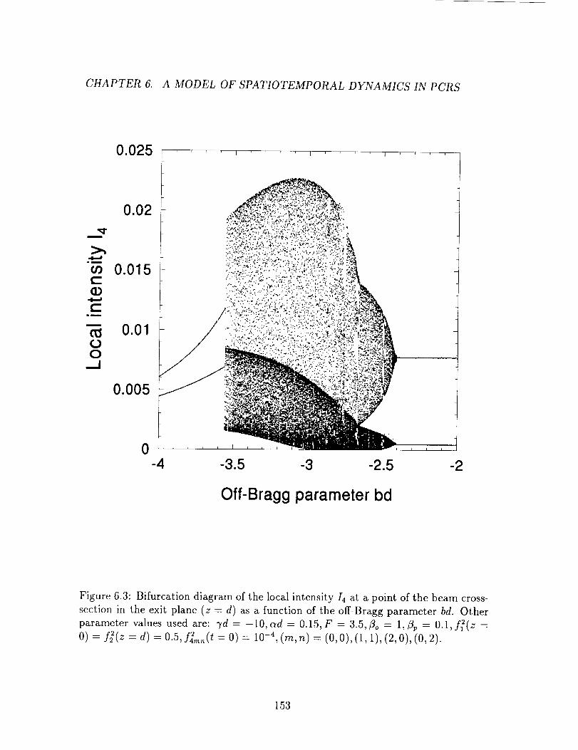
CHAPTER 6. A MODEL OF SPATIOTEMPORAL DYNAMICS IN PCRS
m
¢.0¢-Q
t-im
00
0.025
0.02
0.015
0.01
0.005
[ I
0-4 -3.5 -3 -2.5 -2
Off-Bragg parameter bd
Figure 6.3: Bifurcation diagram of the local intensity/4 at a point of the beam cross-
section in the exit plane (z = d) as a function of the off-Bragg parameter bd. Other
parameter values used are: 7d = -10, ad = 0.15, F = 3.5, flo = 1,tip = 0.1,f_(z =
O) = f_(z = d) = 0.5, f_mn(t = O) = 10-4, (re, n) = (0,0), (1, 1), (2,0), (0,2).
153

CHAPTER 6. A MODEL OF SPATIOTEMPORAL DYNAMICS IN PCRS
1 i I ' ' IoI-1-2-3-4-5 k i i L i i i L I i F i _ i i i i , ,' 0.5 1 1.5 2
O_ f2 fl f +f 2f1 (b) bd= -2.45
' 0.5 1 1.5 22 1 .... ,f .... , .... , ....
O_ f2 = f _1 fl+f2 2fl (c) bd=-2.55-I nl- 2
if) -3
_0 0.5 1 1.5 21
13-0
----_ -3-4-510
-1-2-3-4-5
, , _ ' L,I: _ ' _ ' I ' ' ' I ' ' ' '
;- f2 /1 (d) bd= -2.75
i _ I I I i I i _ I L L i i I
tiff 15
-fl/13 fl ' (ei bd=-'3.i8-_
1
F .
0.5 1 1.5 Z
frequency
Figure 6.4: Power spectra of the time series of fig. 6.2 illustrating the dynamics as
the off-Bragg parameter bd is varied. (a) a periodic motion with a single frequency,
(b) quasiperiodic motion with two (relatively) incommensurate frequencies, (c) same
with more energy in the side bands, reflecting the deeper modulation of fig. 6.2c, (d)
broadening of the two frequency peaks and their harmonics with the appearance of
an additional low frequency leading to chaotic motion, (e) two frequency peaks of
commensurate ratio corresponding to frequency locking at period 13.
154
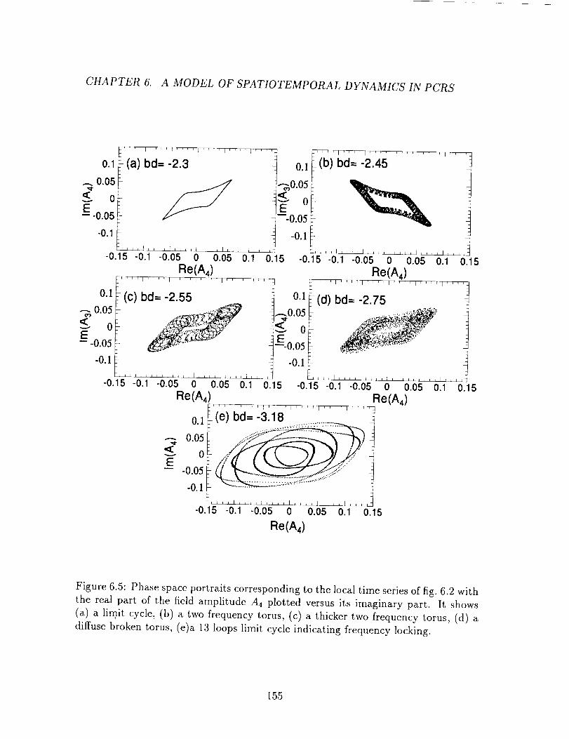
CHAPTER 6. A MODEL OF SPATIOTEMPORAL DYNAMICS IN PCRS
0.1
_. 0.05
0
IE-0.05
-0.1
.... l''''p .... I''' 'I .... I'''
(a) bd= -2.3
0.1
.--. 0.05O_
'( 0E-- -0.05
_,,,I,,, LrL,,,I, ,_,iL_,jl,kL,-0.11-0.1-0.05 0 0.05 0.1
Re(A,,,)_f'' ,I ,T,,l_r, ,Ir,,,[,,,, F ,
(c) bd= -2.55
5{ ,,/" "
-0.15
-0.1
''''l'L''l_'L'll,,LIJllkl_-0.1 -0.05 0 0.05 0.1
Re(A4)
0.15
0.1
---- 0.05
oE-- -0.05
-0.1
-0.11
i i r_
0.1
_r_ _ ,[ .... I .... [ r r, _ I .... 14,,
(b) bd=-2.45
o_--E_o.os -
-0.1 _-
0.15
•"-_0.05 i
---0.05 E-
-0.1
-0.15 -0.1 -0.05 0 0.05 0.1 0.15
Re(A4)
(d) bd=-2.75 .....,.::,,,","-_:
i'(' ')f I .... I .... I .... p .... i,m,e bd= -3.18
,:-:..J.,.,,._:._,-._._._:' ..........._32....
;. .......
-0.1 -0.05 0 0.05 0.1 0.15
Re(A4)
_iJ_liiii&lctrililiilli¢_lull r
-0.15 -0.1 -0.05 0 0.05 0.1 0.15
Re(A4)
Figure 6.5: Phase space portraits corresponding to the local time series of fig. 6.2 with
the real part of the field amplitude A4 plotted versus its imaginary part. It shows
(a) a limit cycle, (b) a two frequency torus, (c) a thicker two frequency torus, (d) a
diffuse broken torus, (e)a 13 loops limit cycle indicating frequency locking.
155
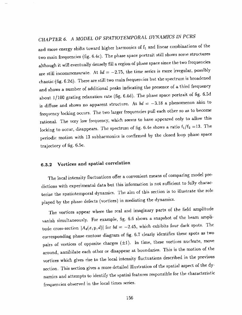
CHAPTER 6. A MODEL OF SPATIOTEMPORAL DYNAMICS IN PCRS
and more energy shifts toward higher harmonics of fl and linear combinations of the
two main frequencies (fig. 6.4c). The phase space portrait still shows some structures
although it will eventually densely fill a region of phase space since the two frequencies
are still incommensurate. At bd = -2.75, the time series is more irregular, possibly
chaotic (fig. 6.2d). There are still two main frequencies but the spectrum is broadened
and shows a number of additional peaks indicating the presence of a third frequency
about 1/100 grating relaxation rate (fig. 6.4d). The phase space portrait of fig. 6.5d
is diffuse and shows no apparent structure. At bd = -3.18 a phenomenon akin to
frequency locking occurs. The two larger frequencies pull each other so as to become
rational. The very low frequency, which seems to have appeared only to allow this
locking to occur, disappears. The spectrum of fig. 6.4e shows a ratio fl/f2 =13. The
periodic motion with 13 subharmonics is confirmed by the closed loop phase space
trajectory of fig. 6.5e.
6.3.2 Vortices and spatial correlation
The local intensity fluctuations offer a convenient means of comparing model pre-
dictions with experimental data but this information is not sufficient to fully charac-
terize the spatiotemporal dynamics. The aim of this section is to illustrate the role
played by the phase defects (vortices) in mediating the dynamics.
The vortices appear where the real and imaginary parts of the field amplitude
vanish simultaneously. For example, fig. 6.6 shows a snapshot of the beam ampli-
tude cross-section IA4(x,y,d)] for bd = -2.45, which exhibits four dark spots. The
corresponding phase contour diagram of fig. 6.7 clearly identifies these spots as two
pairs of vortices of opposite charges (-4-1). In time, these vortices nucleate, move
around, annihilate each other or disappear at boundaries. This is the motion of the
vortices which gives rise to the local intensity fluctuations described in the previous
section. This section gives a more detailed illustration of the spatial aspect of the dy-
namics and attempts to identify the spatial features responsible for the characteristic
frequencies observed in the local times series.
156

CHAPTER 6. A MODEL OF SPATIOTEMPORAL DYNAMICS IN PCRS
2
1
0
-1
-2 -2
bd= -2.45, t=1502.81:'
0
2
Figure 6.6: The profile of the absolute value of the field amplitude ]A41 showing fourholes in the beam cross-section.
157

CHAPTER 6. A MODEL OF SPATIOTEMPORAL DYNAMICS IN PCRS
2bd= -2.45
1 1.8_:
0
0
-1
0
8/I;
-2-2 -1 0 1 2
x/to o
Figure 6.7: Phase contour map corresponding to the amplitude map of fig. 6.6 clearly
identifies the four holes in the wavefront as two pairs of vortices of opposite charges
(+1).
158

CHAPTER 6. A MODEL OF SPATIOTEMPORAL DYNAMICS IN PCRS
(C) ' ..... ,,.. (d) -I "' _l, '
(o) , -' _'_. ' '
--z
Figure 6.8: Time evolution of the modulus of the field amplitude A4 along a line z = 1
for different values of the off-Bragg parameter bd, showing (a) a synchronized periodic
motion, (b) a periodic motion with transverse modulation, (c) a quasiperiodic motion,(d) a turbulent flow, (e) another periodic flow.
159

CHAPTER 6. A MODEL OF SPATIOTEMPORAL DYNAMICS IN PCRS
Figure 6.8a to e shows the temporal evolution of the modulus of the field amplitude
A4(x = 0.75, y, d) along a line across the beam for the same off-Bragg parameter values
used in figs. 6.2, 6.4, 6.5. For a small offset (bd = -2.3), all points across the line
execute synchronized periodic motions with a period a bit smaller than two grating
time constants (fig 6.8a). In 2-D, the phase of the wavefront is observed to breathe
periodically together with the amplitude but the phase gradients produced are not
steep enough to trigger the nucleation of defects.
At bd = -2.45 (fig 6.8b), the periodic motion is transversely modulated with a
period of the order of 10 grating time constants. This spatial motion gives rise to
the quasiperiodic time series of fig. 6.2b. In 2-D, the phase gradients are locally
steep enough to tear the wavefront at locations where two pairs of defects of opposite
charges nucleate. The four vortices then travel across the wavefront, and pairs of
opposite charge collide and annihilate. The higher frequency of the time series seems
to correspond to the recovery rate of the local wavefront after a vortex has moved
through it, while the lower frequency corresponds to the full cycle of vortex nucleation,
motion and annihilation. At bd = -2.55, the motion is similar to that just described
but with deeper modulation (fig. 6.8c, which is plotted with a different time scale).
At bd = -2.75 (fig. 6.8d), the transverse modulation is irregular, possibly due to
the occurrence of a third incommensurate frequency. In 2-D, in contrast with the
previous case where the vortices' trajectories were confined to a fairly well defined
area, they now seem to visit the whole beam cross-section irregularly. At bd = -3.18
(fig. 6.8e) the motion is periodic again. The transverse modulation has a period of
_-, 23 grating time constants, which is 13 times the period of ,-_ 9/5 time constant of
the fast oscillations measured in fig. 6.8a.
The remainder of this section gives a more detailed illustration of the relationship
between the vortices' trajectories and the spatiotemporal coherence of the beam.
The dynamics of the fluctuating beam can be characterized by a correlation index
distribution calculated from the spatial correlation function defined in eq. 5.4.
To illustrate the usefulness of this concept, the correlation index distribution with
160

CHAPTER 6. A MODEL OF SPATIOTEMPORAL DYNAMICS IN PCRS
respect to the origin, C(O,O;z,y), was calculated for the five off-Bragg parameter
values used in the previous examples. The spatial correlation diagram thus obtained
can then be compared with the vortices' trajectories. For this, the positions of the
vortices were calculated at regular intervals of time by solving for ReA4(x,y,t ) =
ImA4(z, y, t) =0, and they are represented by dots on a 2-D plot. Note in passing
that, with the particular choice of modes adopted for the expansion of A4, these
positions could be solved for algebraically.
Figure 6.9 shows the correlation index distribution for a small value of the off-
Bragg parameter (bd = -2.3). No vortices appear in the field but the amplitude
and phase of the wavefront oscillate periodically as if waves were travelling along an
annular area centered on the beam.
At bd = -2.45, the motion is characterized by the nucleation of two pairs of
defects at two diagonal ends. The vortices move along circular trajectories and the
members with opposite charges from each different pair collide and annihilate near
the two diagonal ends on the other side. This motion is then repeated periodically
with alternating directions. A sequence of interferogram snapshots illustrating this
motion is shown in fig. 6.10. A plot showing the distribution of vortice's positions in
time is shown in fig. 6.11a. The vortices' trajectories are clearly confined to a narrow
annular area in the beam. Figure 6.11b shows the corresponding correlation index
distribution. Its particular shape can be explained by the fact that the intensity fluc-
tuations at some location in the beam are due to the passage of a vortex nearby, that
no vortex ever appears near the origin (the fixed point for calculating C) and that the
vortices' trajectories are confined to a narrow annular region of space. It is only near
this region that the correlation index is expected to drop sharply. The correlation in-
dex distribution was also calculated with a fixed point chosen at a location frequently
visited by a vortex. The relationship between the distributions of fig. 6.11a and b
is analogous to that between a photographic print and its negative. The correlation
index is high in the annular area visited by the vortices and low everywhere else. This
confirms that the four vortices appearing in the pattern are highly correlated, as is
expected since they nucleate simultaneously and produce intensity fluctuations near
161
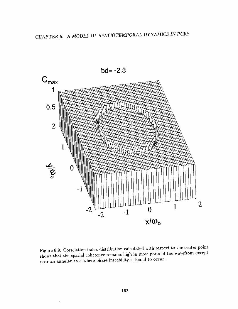
CHAPTER 6. A MODEL OF SPATIOTEMPORAL DYNAMICS IN PCRS
Cmax
1
bd= -2.3
2
1
o
0
X/COo
1 2
Figure 6.9: Correlation index distribution calculated with respect to the center point
shows that the spatial coherence remains high in most parts of the wavefront except
near an annular area where phase instability is found to occur.
162
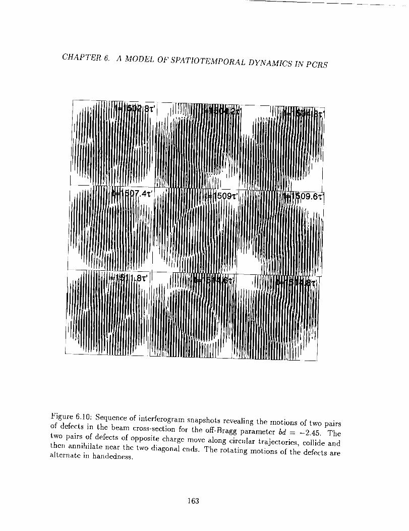
CHAPTER 6. A MODEL OF SPATIOTEMPORAL DYNAMICS IN PCRS
Figure 6.10: Sequence of interferogram snapshots revealing the motions of two pairs
of defects in the beam cross-section for the off-Bragg parameter bd = -2.45. The
two pairs of defects of opposite charge move along circular trajectories, collide and
then annihilate near the two diagonal ends. The rotating motions of the defects arealternate in handedness.
163

CHAPTER 6. A MODEL OF SPATIOTEMPORAL DYNAMICS IN PCRS
0
3 0
(a)
(b)
2 _, ' ' I .... I ' ' ' ' I ' ' ' ' ]
-1
bd= -2.45:
_.'"._'_ _" ;'. ,.
k I
- -1 0 1 2
X/(_O
Cr,,,, bd= -2.451
0.5
2
1
"_ o0
2
-2 -2 -1X/tOo
Figure 6.11: (a) Trajectories of defects in the wavefront for the off-Bragg parameter
bd = -2.45, localized on an annular ring. (b) The correlation index with respect to
a point at beam center drops sharply near the defects' trajectories.
164
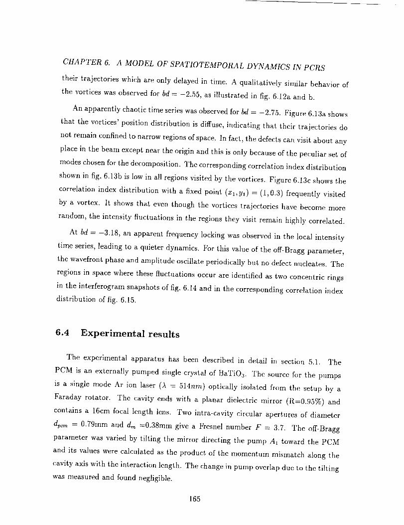
CHAPTER 6. A MODEL OF SPATIOTEMPORAL DYNAMICS IN PCRS
their trajectories which are only delayed in time. A qualitatively similar behavior of
the vortices was observed for bd = -2.55, as illustrated in fig. 6.12a and b.
An apparently chaotic time series was observed for bd = -2.75. Figure 6.13a shows
that the vortices' position distribution is diffuse, indicating that their trajectories do
not remain confined to narrow regions of space. In fact, the defects can visit about any
place in the beam except near the origin and this is only because of the peculiar set of
modes chosen for the decomposition. The corresponding correlation index distribution
shown in fig. 6.13b is low in all regions visited by the vortices. Figure 6.13c shows the
correlation index distribution with a fixed point (xl,yl) = (1, 0.3) frequently visited
by a vortex. It shows that even though the vortices trajectories have become more
random, the intensity fluctuations in the regions they visit remain highly correlated.
At bd = -3.18, an apparent frequency locking was observed in the local intensity
time series, leading to a quieter dynamics. For this value of the off-Bragg parameter,
the wavefront phase and amplitude oscillate periodically but no defect nucleates. The
regions in space where these fluctuations occur are identified as two concentric rings
in the interferogram snapshots of fig. 6.14 and in the corresponding correlation index
distribution of fig. 6.15.
6.4 Experimental results
The experimental apparatus has been described in detail in section 5.1. The
PCM is an externally pumped single crystal of BaTiOa. The source for the pumps
is a single mode Ar ion laser ()_ = 514nm) optically isolated from the setup by a
Faraday rotator. The cavity ends with a planar dielectric mirror (R=0.95%) and
contains a 16cm focal length lens. Two intra-cavity circular apertures of diameter
dpcm = 0.79mm and dm =0.38mm give a Fresnel number F = 3.7. The off-Bragg
parameter was varied by tilting the mirror directing the pump A1 toward the PCM
and its values were calculated as the product of the momentum mismatch along the
cavity axis with the interaction length. The change in pump overlap due to the tilting
was measured and found negligible.
165
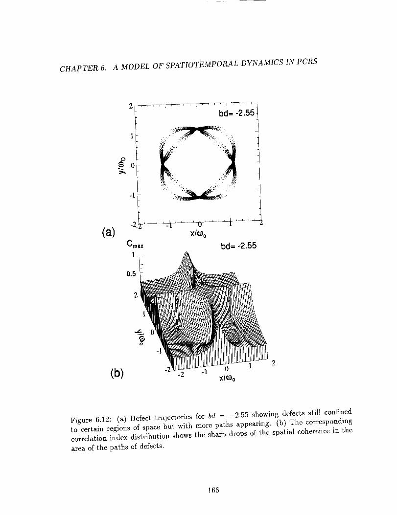
CHAPTER 6. A MODEL OF SPATIOTEMPORAL DYNAMICS IN PCRS
2
(a)
(b)
0
3 0
-1
bd-- -2.55
-:,:___:,; :.:..../- .:_,e_.- "_?,_ : ,
",,;I,"
:.., . %.. ,..;s'.'- .' .".; -
-2.x/(,Oo
Cmax
1
0,
o
-2
bd= -2.55
2
Y,l(.Oo
Figure 6.12: (a) Defect trajectories for bd = -2.55 showing defects still confined
to certain regions of space but with more paths appearing. (b) The corresponding
correlation index distribution shows the sharp drops of the spatial coherence in the
area of the paths of defects.
166

CHAPTER 6. A MODEL OF SPATIOTEMPORAL DYNAMICS IN PCRS
2.... . r .... F .... i ,' ' _ '
.....,,-, bd=-2.75
"" -""i": "" "' :"i "_':,< """ *"; • "
C" "::]:):,.._ 7_ _!1 _0:,.:". :,.... :... _,.".. ._:,_ _:_'- ,.
" ..:_.:_<"....q:,_...,_',_'_ ':."_d_.':..... C" '
-2 , , , , [ i , , , j , , , , [ ., , , ,-2 -1 0 1
x/o 0
0
ao
(a)Cmax
0.5
2
1
-2(b)
2
bd- -2.75 _,IE
0 1 bd= -2.75
2
0.5
2
1
..,,,
-2 0 1 2
(c) -2 Joo
Figure 6.13: (a) At bd = -2.75, the defect trajectories become more diffuse and
occupy larger regions of space in the wavefront. (b) The correlation index distribution
with respect to the center point drops to small values at places where the defects
concentrate. (c) The correlation index distribution with respect to a point (1,0.5)shows a high spatial coherence in all areas visited by the defects.
167

CHAPTER 6. A MODEL OF SPATIOTEMPORAL DYNAMICS IN PCRS
Figure 6.14: Sequence of snapshots of interferograms showing the time evolution ofstructures in the beam cross-section at bd = -3.18. It shows fringes bending with no
defect nucleation. The phase breathes periodically in two concentric annular areas.
168

CHAPTER 6. A MODEL OF SPATIOTEMPORAL DYNAMICS IN PCRS
Cmax bd= -3.18
1
0.5
2
o
1
0
-2 0 1-2 -1 X/O_o
2
Figure 6.15: The correlation index distribution with respect to the center point show
a structure with two concentric rings. The regions of low values of the correlation
index are the places where fringe bendings are observed.
169
CHAPTER 6. A MODEL OF SPATIOTEMPORAL DYNAMICS IN PCRS
The aim of the experiments is to show, by way of illustration, that the range of
behaviors predicted by the model and described in section 6.3 is indeed observed in
the physical system. It would be unrealistic to expect a quantitative match between
the experimental data and the results of numerical simulations if only because it is
not possible to control experimentally which modes are actually taking part in the
dynamics. A qualitative match, however, would at least indicate that the truncated
modal expansion approach gives a fair representation of the actual dynamics of the
PCR.
Figure 6.16 shows an interferogram snapshot of the beam exiting the PCM. It
exhibits four vortices located at the corners of a quadrangle in an arrangement similar
to that predicted by the model in figs. 6.6 and 6.10.
The off-Bragg parameter was scanned between two extreme values at which the
momentum mismatch is large enough to reduce the gain below cavity losses and pre-
vent oscillation. Local time series were recorded within that range and analyzed using
power spectra and delayed-time phase space portraits. Near the center of the cov-
ered range of parameter values, a region where the motion was clearly periodic could
be identified. On both sides of this region, similar sequences of various dynamical
behaviors were observed, up to large mismatches at which the cavity stops oscillat-
ing. Before reaching these limits, simple periodic oscillations at reduced amplitudes
were again observed. The sequence of behaviors just described is exactly what the
bifurcation diagram of fig. 6.3 would predict (note that within the approximations of
the model, this bifurcation diagram is symmetrical around bd = 0, but in the actual
setup this symmetry is broken). By analogy with the model, the origin of parameter
space (bdr = 0) was chosen as the midpoint of the central region showing periodic
oscillations. Other values of the off-Bragg parameter mentioned below are relative to
this point. Some examples of time series are shown in fig. 6.17 and the corresponding
power spectra are displayed in fig. 6.18. These examples were chosen to illustrate the
variety of dynamical behaviors exhibited by the PCR and to compare them with the
characteristic behaviors predicted by the model.
Figures 6.17a, 6.18a show the periodic motion expected for the off-Bragg parameter
170
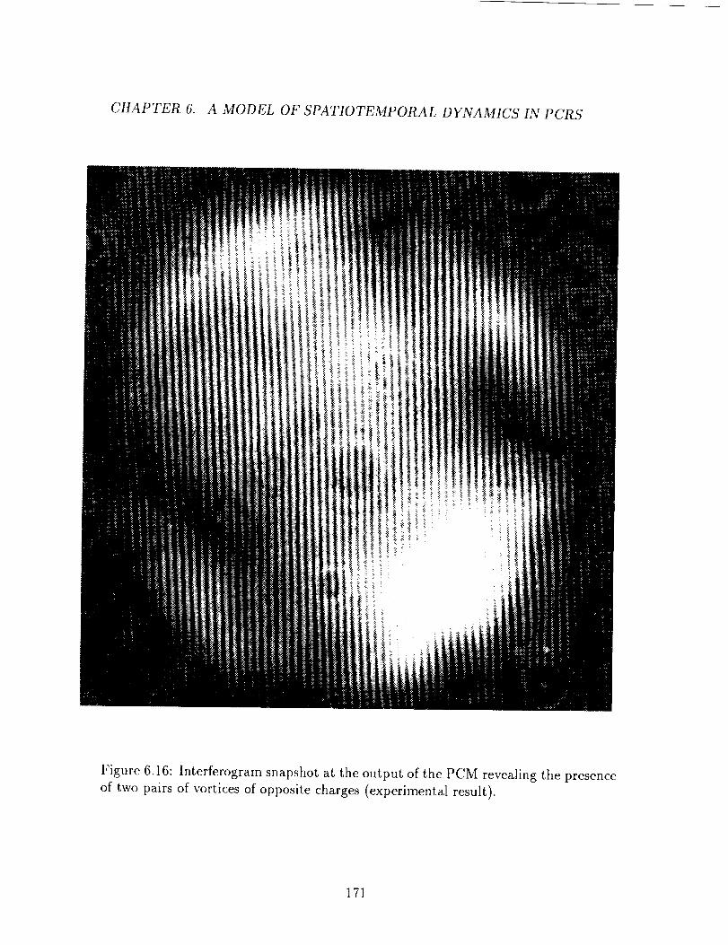
CHAPTER 6. A MODEL OF SPATIOTEMPORAL DYNAMICS IN PCRS
Figure 6.16: Interferogram snapshot at the output of the PCM revealing the presence
of two pairs of vortices of opposite charges (experimental result).
171
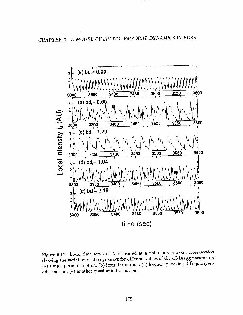
CHAPTER 6. A MODEL OF SPATIOTEMPORAL DYNAMICS IN PCRS
3
2
_" 3300 3350 3400 3450 3500 3550 3_00
>', 3 -(c)Odr=1.29 .......2
I::
.(::: 3300 3350 3400 3450 3500 3550 3600
3
00 2
._1 !
3300 3350 3400 3450 3500 3550 3600i i i i i i i i t i i i * i 1 i J '
3
2
]
3300 3350 3400 3450 3500 3550 3_00
time (sec)
Figure 6.17: Local time series of/4 measured at a point in the beam cross-section
showing the variation of the dynamics for different values of the off-Bragg parameter:
(a) simple periodic motion, (b) irregular motion, (c) frequency locking, (d) quasiperi-
odic motion, (e) another quasiperiodic motion.
172
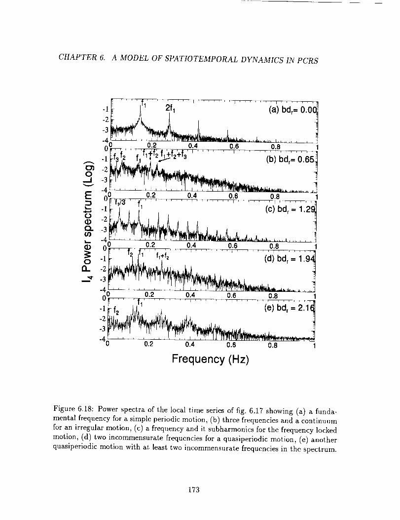
CHAPTER 6. A MODEL OF SPATIOTEMPORAL DYNAMICS IN PCRS
-'I....A"'2';'.............i.),:,<,;-oo,ii
-_o 0.2 o._'""";"_-o.8.........o8 "' :,"Fi.f;", 'fi,+f2fl_-f_-f_'' ....... ' ...... ,;.i;.;,' ',_:..,;_
A .I, .t_l .iAl.,t,i_,Li ,_ h=
"_0 0.2 0.4 0.6 ..... ' 0 8 ........ 1u_,fv_ ' ',, , r ....... i ....... , ....... i ........
1I1"' l 1i -!, , (c) bd r=1.29_
_34"2 1
0_ -011 J_l.,Ifli fill'f2 [ , .... (di bdr'- i .'9'_
m -3
/ -..,x i ll,,,_..i. ..... !
-4 0 2 0.4 0.6 0.8 - :
"1_-'f2 ,J,AI1 ' (e) bdr=2'16
-41-' ...... ' ....... _,_-_.._._0.2 0.4 0.6 0.8
Frequency (Hz)
Figure 6.18: Power spectra of the local time series of fig. 6.17 showing (a) a funda-
mental frequency for a simple periodic motion, (b) three frequencies and a continuum
for an irregular motion, (c) a frequency and it subharmonics for the frequency locked
motion, (d) two incommensurate frequencies for a quasiperiodic motion, (e) another
quasiperiodic motion with at least two incommensurate frequencies in the spectrum.
173
CHAPTER 6. A MODEL OF SPATIOTEMPORAL DYNAMICS IN PCRS
bd = 0. The corresponding delayed-time phase space portrait (fig. 6.19a) shows
broadening which may give an indication of the level of stochastic noise.
Figures 6.17b, 6.18b obtained with bdT = 0.65 show a chaotic state with an ir-
regular time series and a spectrum containing at least two or three incommensurate
frequencies, including the main frequency of about 0.14Hz, and a broad continuum,
a signature of chaos. The exponential decay of the power spectrum (linear on the
semilog scale of fig. 6.18) may be indicative of deterministic chaos. The corresponding
phase space portrait of fig. 6.19b is diffuse and essentially featureless.
Figures 6.17c, 6.18c give a typical example of frequency locking obtained at bdT =
1.29. The locking at period three is confirmed by the closed-loop phase space trajec-
tory shown in fig. 6.19c. Note that the width of this limit cycle is about the same as
that of fig. 6.19a and is probably due to stochastic noise.
At bd_ = 1.94 (figs. 6.17d, 6.18d) the motion is quasiperiodic with a spectrum
containing only two incommensurate frequencies and their linear combinations. An-
other quasiperiodic motion obtained at bdr = 2.16 is shown in fig. 6.17e, 6.18e. Here
the lower frequency appears as sidebands of the higher one. For larger values of the
off-Bragg parameter, e.g. bdr > 2.37, the motion is periodic again with the same
dominant frequency of _ 0.14Hz but with decreasing amplitude. When bd_ > 3, the
gain is lower than the cavity losses and no oscillation occurs.
6.5 Summary and conclusions
A model based on a truncated modal expansion of the cavity modes has been
tested to describe the spatiotemporal dynamics of a phase-conjugate resonator. The
Gauss-Hermite modes of the empty cavity are chosen as sensible basis functions to
represent the fields in the nonlinear medium. Although the choice of the modes
which take part in the dynamics is arbitrary in this method, justifications are given
for truncating the series at a mode index of the order of the cavity Fresnel num-
ber. Verification of the validity of this choice are later given by comparison with
174

CHAPTER 6. A MODEL OF SPATIOTEMPORAL DYNAMICS IN PCRS
2.5
(a)bd,- 0.00
A
1.5m
0.5
o0 .... o15.... I_.... I.'5.... 2' .... 2.5'.... 3
14(n)
(c)bd r = 1.29
2.5
2
,; J-
+t= 1.5 -:,,,
I r . " ,'_ ' ,"
j ;Si::i::0 .... r .... L , . , i
0 0.5 1 1.5 2 2.5
(b) t,(n)
3 - • • , .... , rr
(d)bd r - 1.94
2.5
-,. .,:I"_'c, - - ,e.
0.5 - _,_.-_ %,_,_
0 .... _ , , ,
0 0.5 1 1.5 2 2.5
(d) i,,(nl
Figure 6.19: Time delayed phase-space portraits obtained from the data of the time
series in fig. 6.17 showing (a) a limit cycle, (b) an irregular distribution, (c) a cycle-three motion, (d) smeared trajectories for the quasiperiodic motion.
175

CHAPTER 6. A MODEL OF SPATIOTEMPORAL DYNAMICS IN PCRS
experimental data. Numerical examples, using the off-Bragg parameter (momentum
mismatch) as a control parameter, reveal a rich variety of dynamical behaviors illus-
trated by the local intensity fluctuations and ranging from simple periodic oscillations
to quasiperiodic motions and chaotic states.
The modal decomposition method is particularly well suited to studying the spa-
tial aspect of the dynamics without requiring prohibitive computational budgets.
Numerical results indicate that the spatiotemporal dynamics of the PCR is mediated
by the nucleation of pairs of defects of opposite charges in the beam and by their sub-
sequent motion and annihilation. Maps of the spatial coherence function of the beam
are found to be templates of the corresponding maps of the vortices' trajectories,
establishing a strong correlation between these two quantities. The loss of temporal
coherence and the onset of temporal chaos in the local intensity fluctuations is like-
wise correlated to the loss of spatial confinement of the vortices' trajectories and to
the loss of spatial coherence.
Experimental data obtained with a PCR, using an externally pumped BaTiO3
photorefractive PCR, reveal a range of dynamical behaviors similar to those shown
by the simulation. These results confirm and complete the findings of the earlier
experimental study of the PCR's dynamics at various Fresnel number, given in chapter
5. The arbitrariness of choice of the modes to include in the dynamics is the main
shortcoming of the truncated modal expansion approach. Nevertheless it appears to
be a convenient and computationally nondemanding tool to use to study and predict
qualitatively the spatiotemporal behavior of phase-conjugate resonators and perhaps
of other nonlinear optical devices as well.
176

Chapter 7
Conclusion
7.1 Discussion and summary
The material presented in this thesis is the result of an inquiry about the possible
use of a phase conjugate resonator (PCR) as an image storage as well as a processing
element in structural control (e.g. for the real time monitoring of the deformation
of large structures). The dynamics of the PCR has been studied in two distinct
regimes. Below threshold (gain < loss), the PCR cannot self-oscillate. In this regime,
the output beam is always stationary in space and time, after the transients have died
out. This stability makes it possible to use the PCRs in image processing applications.
When the gain threshold is exceeded (above threshold), the PCR self-oscillates and
spatiotemporal instabilities in the output beam set in.
This thesis was thus organized in two parts. In the first part, we have investigated
the transient behavior and stability properties of a PCR below threshold. In the sec-
ond part, we have studied experimentally and theoretically the PCR's spatiotemporal
dynamics above threshold.
We have presented the transient dynamics of a PCR below threshold based on
time-dependent coupled wave equations for FWM in a photorefractive crystal with
two distinct interaction regions caused by the feedback from a slightly tilted ordi-
177
CHAPTER 7. CONCLUSION
nary mirror. First, we have solved the steady state equations for the cavity's fields
analytically, assuming nondepleted pumps and an absorption free medium. The so-
lutions predict that the PCR self-oscillates (reaches threshold) in a broader range
of values of pump ratios if the PCM has a higher values of the coupling parameter.
The PCR's transfer function (below threshold) is obtained through applying a sim-
ple frequency-domain transformation technique to the steady state equations. The
transfer function is shown to be largely dependent on the coupling parameter and the
pump ratio. Contour plots of the transfer function as a function of complex angular
frequency indicate that there is no sign of instability before the PCR can self-oscillate,
while unstable poles quickly develop once the PCR is above threshold.
In the transient regime of the PCR, we have successfully applied a numerical
scheme for integrating the photorefractive FWM equations separately in the space
and the time domains using the adiabatic elimination process. Numerical calculations
of the cavity's buildup and decay times as well as of the specularly reflected and
phase conjugate reflected intensities as functions of a number of system parameters
confirm that the parameters affecting the threshold most directly are the coupling
parameter and the pump ratio. We have presented results which indicate that the
cavity buildup and decay times can be tailored by varying several system parameters.
Results predict the possible use of the PCR as an image processing element. For
example, the PCR could, in principle, perform constrast enhancement during buildup
and contrast reduction during decay. This same feature could be used to implement a
time varying spatial filtering if the projected field in the PCM is the spatial spectrum
of an image rather than the input image itself. Experimental measurements of the
cavity's buildup and decay times confirm qualitatively the result of the numerical
simulations.
In the above-threshold regime, we have studied experimentally some aspects of the
spatiotemporal behaviors of the PCR as a function of the Bragg detuning bd achieved
by misaligning one of the two pump beams, and as a function of the degree of trans-
verse confinement controlled by varying the resonator's Fresnel number F. Temporal
aspects of the beams' complexity were revealed by analysing the local intensity time
178
CHAPTER 7. CONCLUSION
series, power spectra, and embedded phase space portraits. In the case of varying F,
we observed bifurcation phenomena typical of low dimensional dynamical systems, i.e.
in order of increasing control parameter, a bifurcation from a stationary to a periodic
state, followed by more subharmonic bifurcations, the occurrence of a chaotic state,
the occurrence of intermittency, and finally a fully turbulent state. For a particular
case of irregular oscillations, the correlation dimension of the attractor constructed
from the embedded phase space was calculated to be approximately 5.2, indicating
that the attractor may be strange. Furthermore, a positive finite lower bound value
of the Kolmogorov entropy can be extracted from the same time series, indicating the
existence of a deterministic chaos. In the case of varying bd, the temporal aspects of
the dynamics in the local time series range from simple periodic oscillations, followed
by quasiperiodic states interrupted by chaotic states. All experimental results thus
far have consistently revealed the presence of two distinct frequencies in the power
spectra in some regions of parameter space.
Regarding the spatial aspects of the beams' complexity, we have demonstrated the
existence of wavefront dislocations or vortices in the optical fields by video recording
and by interferometry. A rich variety of defect movements has been recorded and
analysed. The spatial complexity was characterized by the number of optical vortices
and their variety of movements, as well as by their relationship with the beam's
spatial coherence. The number of defects and the spatial correlation index have been
shown to follow similar trends as the transverse confinement of the system is relaxed,
pointing to the role played by the wavefront dislocations in the dynamics.
We have also tested a model based on a truncated modal expansion of the cavity
modes, to investigate the spatiotemporal dynamics of the PCR. We have clearly shown
that the optical vortices in the wavefront are also present in the numerical solutions.
Simulations using the Bragg detuning as a control parameter have shown that optical
vortices begin to appear under conditions of increased local gain which appears to be
obtained by the small misalignment of one of the pump beams from the Bragg angle.
Power spectra of simulated time series also contain two distinctive frequencies for a
certain range of the off-Bragg parameter, indicating that the dynamics is governed

CHAPTER 7. CONCLUSION
by two different time scales. The short one, on the order of the material's damping
time, seems to correspond to the recovery rate of the local wavefront after a vortex
has moved through it, while the long one is associated with the alternation from one
mode to another in the competition process and seems to correspond to the full cycle
of the vortices' nucleation, motion and annihilation. Numerical results also indicate
that the loss of temporal coherence and the onset of temporal chaos in the local
intensity fluctuations is likewise correlated to the loss of spatial confinement of the
vortices' trajectories and the spatial coherence.
Thus far, several reports have been published in the literature concerning tem-
poral instabilities in photorefractive oscillators. Each of these systems has provided
a physical picture of how chaotic oscillations can occur. Our study shows that the
spatiotemporal chaotic behaviors in a PCR may possibly be attributed to the mech-
anisms of the competition among various cavity modes and the gain enhancement
which arises from off-Bragg FWM. As we have seen in chapter 2, the steady state
solution predicts that the range of pump ratios Rp, within which the feedback param-
eter _ can be greater than one, becomes wider and wider as the coupling parameter
%d is increased. The direct numerical integration of the FWM equations in chapter 3
confirms that the PCR can fall into the above-threshold regime in a wider range of
pump ratios with increasing values of the coupling parameter. In chapter 6, we pre-
sented the three dimensional FWM equations in order to account for the transverse
dynamics in the PCR. We introduced a modal decomposition method in which cav-
ity fields are basically described by a set of participating cavity modes. Numerical
results show that chaotic oscillations set in for a large enough coupling parameter
(e.g. I%dl > 8). In the modal decomposition method, we have seen how the modal
amplitudes of the cavity fields are coupled to each other in eqs. 6.20-6.23. It is this
complex coupling that brings about the unstable oscillations which would otherwise
not be seen in the plane-wave FWM model even in cases of quite large coupling pa-
rameters. The off-Bragg parameter bd obtained by tilting one of the two pumps away
from the Bragg angle is another significant factor in lowering the threshold for the
instabilities observed in PCR. When bd = 0 (no Bragg detuning), only periodic os-
180
CHAPTER 7. CONCLUSION
cillations are seen in the output. When bd _ 0 (with Bragg detuning), quasiperiodic
and irregular oscillations appear in the output.
With no Bragg detuning, the coupling between cavity modes provides only chan-
nels for energy exchange between modes. This "beating" between oscillating modes
leads to periodic changes in the output beam. With Bragg detuning, there is an
additional phase transfer between the interacting modes due to the additional phase
shifts of the individual mode gratings. It is this coupling of the phases which makes
possible the occurrence of chaotic behavior. An intuitive explanation for this behavior
is the following. Consider what happens inside the crystal as the FWM process pro-
gresses in time. Initially pump 2 illuminates the crystal and at time t = 0 pump 1 is
turned on and scattered noise in the cavity forms beam 4. Then, beam 1 and beam 4
start to write various mode gratings and beam 2 is scattered from these gratings and
the scattered beam is fed back from the dielectric mirror. However, as the gratings
start to form, they change the phase of the individual mode. This in turn causes a
new mode grating to be written, which again changes the phases of the participating
modes, and so on. This constant change in phases of the interacting beams leads to
constantly writing new gratings and washing out old gratings. It is these dynamic
gratings together with the feedback of the cavity that gives rise to chaotic oscillations
once some gain threshold is exceeded.
A final remark should be given. The arbitrariness of choice of the participating
modes is the main shortcoming of the truncated modal expansion approach used in
this work, despite the fact that justifications are given for truncating the series at a
mode index of the order of the cavity Fresnel number. Yet, the method is shown to
be a particularly convenient and computationally nondemanding tool for study of the
spatiotemporal behavior of the PCR and perhaps of other nonlinear systems as well.
Thus far, experimental results are supportive of the validity of this approach.
In conclusion, this the first time to the author's best knowledge that the spa-
tiotemporal dynamics has been both experimentally and theoretically explored in a
photorefractive PCR, and also that direct physical evidence of optical vortices has
been unveiled in detail in the wavefronts of the optical fields from the PCR. Our re-
181

CHAPTER 7. CONCLUSION
sults should prove useful in the study of photorefractive devices and in the assessment
of their practical usefulness. They may also add a small contribution to the growing
area of research in nonlinear dynamics in general.
7.2 Possible future investigations
One of the interesting properties of a PCR is that a great number of transverse
modes is allowed to oscillate if the transverse extent of the cavity is opened up. This
means that an optical processing device utilizing a PCR can have a high spatial
resolution. Yet, the spatiotemporal instabilities due to the transverse mode com-
petition reported in this thesis may impose limitations on the spatial and temporal
performance of the device. To make a device pratical, methods for eliminating these
instabilities are definitely needed. Some efforts have been recently made to alleviate
the spatial and temporal instabilities in a PCR with BaTiOa as the PCM, by using
an intracavity mode homogenizer such as a multimode fiber taper or light pipe [107].
The demonstrated improvement in the spatial and temporal stability, and also the
overall increase in the transverse extent of the oscillating mode, will undoubtedly
make possible many new processing techniques based on PCR in the above threshold
regime.
The mode competition process in the PCM may be favorable for other applica-
tions. For example, associative recall and processing of images using photorefractive
oscillators have already been demonstrated [9, 10, 11]. In these applications, compe-
tition between modes is fundamental for the discrimination capability of the memory.
A recent investigation to explore the possibility of using a laser as a nonlinear ele-
ment in an associative memory architecture [108] may be an important new approach
utilizing the continuous field distributions in a cavity rather than a discrete array of
elements as in many neural networks. One basic requirement for this approach to
be successful is the coexistence of many stable states, or "spatial multistability". In
isolated multistable systems the final state is completely unpredictable because ini-
tial fluctuations determine its evolution. Yet, different behavior is expected when the
182
CHAPTER 7. CONCLUSION
system is driven externally by an identical system. In this case, a weak signal from
the driving system is injected into the system while it is below threshold. As soon
as the injected signal is switched off, the main system is switched above threshold.
The system then starts with the seed left by the signal, and the evolution toward a
stationary state is no longer random but is a function of the spatial configuration of
the initial seed. Still, more demonstrations of practical architectures of such kinds are
definitely needed. It seems that a PCR with high mode volume may be a candidate
for the nonlinear element of an optical associative memory. Nevertheless, the first
question to answer is whether spatial multistability can be achieved in systems based
on photorefractive oscillators. To this end, the PCR patterns must be stabilized and
simultaneously some process must be found to switch from pattern to pattern. Per-
haps the example of using an intracavity mode homogenizer in PCR is a first step
toward achieving these goals.
Another aspect of the spatiotemporal dynamics concerns the behaviors of the cav-
ity fields in other PCR geometries. The similarities and differences obtained with
different setups may be important. At least, with such a comparison we could have
some ideas of what is generic or geometric-specific in the observed dynamics. Fur-
thermore, other new methods for the study of extended systems such as subspace
Lyapunov spectra. [84] could also be applied to the diagnosis of experimental data
from the PCR.
183

Appendix A
Derivation of the four-wave
mixing equations
In this appendix we derive the set of coupled wave equations for waves propagating
in the PCM that are used in studying the dynamics of the PCR. At first we consider
the optical fields as uniform plane waves of infinite extent, then we allow the optical
fields to have transverse spatial variations.
We start with the Maxwell's equations for the macroscopic variables of the fields.
In general these equations take the form:
V×$- _O_ (A.I)cot'
47r --_Vx_- I0/5 + __j,
c Ot c
V. :D = 47rpf,
V./_= 0,
(A.2)
(A.3)
(A.4)
with
_ =/3- 4rA,_,
(A.5)
(A.6)
184

APPENDIX A.
,f : aS, (A.7)
where $ is the total optical electric field, _ is the electric displacement, 75 is the
induced polarization, _ is the magnetic field,/_ is the magnetic induction, ./Q is the
magnetization, p/ is the free charge density, j is the current density, c is the speed
of light in vacuum, ¢o is the permittivity in vacuum, ero is the background (average)
relative dielectric constant when only the pump beams are present, Aer is the relative
induced dielectric constant which is slowly varying in both time and space when both
the pump beams and the probe beams are present, and o" is the conductivity.
For ferroelectric oxides, _ = /_ and p/ = 0. Taking the curl of eq. A.1 and
combining with eq. A.2, we obtain the wave equation:
4rre o%v
c2 Ot '
O_g Ae 02_V2f-d bt f- c 2 Ot 2 + (A.8)
where e = eoero and Ae(r, t) = eoAer. It is assumed that Ae(r, t) is smooth in space
and time. Suppose that the fields inside the PCM are uniform plane waves of the
same polarization, say the extraordinary polarization (see figure A.1). We also assume
that all waves are propagating with small angles to the z-axis and the total intensity
profile as well as the resultant refractive index vary periodically in x with frequency
kx. Thus, we can write down the scalar total optical field in fourier expansion as
oo
g(x,z,t)= y_ A,(z,t)ei(_°':_kzz+'k*_), (A.9)l_--O0
and the induced dielectric constant as
oo
Ae(x,z,t)= _ q(z,t)e _lk==, (A.10)l_--O0
with k_ = koV/-esinO, kz = kox/TcosO, ko = 2rc/to = w/c, where to is the light
wavelength in vacuum.
In the following, we use the slowly varying envelope approximation (SVEA) which
assumes that A_(z, t) and el(z, t) are smooth functions of z and t, i.e.
02 A_ OAl 02At O__zZOt---g-<< 2co 0---7- and Oz---Y <<72k_ . (A.11)
185

APPENDIX A.
-. 0QQ_Q
PCM
A2
'V,
"" A 3
Figure A.I: Schematic diagram for the four-wave mixing geometry. A1 and A2 are
the two external pumps. A4 is the probe beam and Aa is the phase conjugate beam.
Arrows show the beams' polarization and direction of propagation. Beams are sym-
metrical about Z and 0 is the angle inside the crystal, fi denotes the crystal's axis.
186

APPENDIX A.
Substituting eq. A.9 and A.10 with A.11 in A.8 and equating the/th component of
the optical field on both sides, we obtain
OA, we OAt i(1 -/2)k2 27cw_ . iko2
+ c_-kz 0-t + 2-k_ A, + _At = T_- l_' e,,A,-e.(A.12)
In four-wave mixing, without Bragg missmatch, beam 1 is collinear with beam 2 and
beam 4 is collinear with beam 3 (see figure A.1), we have
= = 0 (A.13)
The total optical field as a sum of four beams takes the form
4
g(x,z,t) = _ Aj(z,t)e '(_t-_3.5 (A.14)j=l
Next, for the Bragg's condition in a thick volume hologram situation, i.e. At = 0 for
ill > 1 and A+I -fl 0, eq. A.12 becomes
OA+I wc OA+I ik2o a (A.15)0---7 + C2kz Ot 2kz c+2A:_l - cos----0A+I'
for waves propagating to the right, and
OA+I
OZ
we OA+I ik2o
- + co-i?A±" (A.16)
for waves propagating to the left, where oL = 27c_/Cv_. Thus we can write down the
coupled differential equations for waves propagating inside the PCM in the notation
of figure A.1 as follows:
OA1 1 OA1 -iko c_ (A.17)0_- q- vcos00t - 2v/eCOS0 e2A4 cos0 AI'
OA2 1 OA2 iko
Oz vcos00t - 2x/_cosOe-2A3 + ----d A2'cos (A.18)
OA3 1 OA3 iko a
Oz vcos00t - 2v/_cos0e2A2 + c--_s0A3, (A.19)
OA4 1 OA4 _ -iko c_
O----_+vcosO Ot 2_-s0 c-2A1 cos 0A4' (A.20)
187

APPENDIX A.
with v = Civic. From eq. A.14, the total intensity is
I(x,z,t) = [El 2
A A._-i(g2-g3)._"= Io(z,t) + (m,A_e -'(_'-_')'¢ + _2_3_
+A1A_e-i(fcl-g3)e+ A_A4e -i{;_-_2)'e) + c.c.
(A.21)
with Io(z,t) 4 iAj(z,t)12.= _j=l Because of the small incident angle to the z-axis for
all fields, the exponentials in the 4th and 5th terms are fast changing phase factors
with respect to the slowly varying amplitudes so that they becomes insignificant in
space averaging. Now we let/_1 - k4 = f¢2 - k3 =/(_ with II(_1 _,, 2kx. Then the light
intensity can be written as
I(x,z,t) = Io(z,t) + [I2(z,t)e -ig*': + c.c.], (A.22)
with
h(z,t) = A_(z,t)A*4(z,t) + A_(z,t)A3(z,t). (A.23)
The induced dielectric constant is related to a space-charge field via the linear
electro-optic effect (see Appendix B) and is given by
1 -3A_( x, z, t ) = -_V/-_nor_l l E_( x, z, t ), (A.24)
where rio is the bulk refractive index, r_/f is the electrooptic coefficient, and E_ is
the space-charge field determined by the transport equations B.1-B.4. Also we can
expand the space-charge field in the same form as Ae in eq. A.10:
E_ = Eo + [E2(z,t)e -'K'_ + c.c.] . (A.25)
Thus, comparing eq. A.25 with A.10 and equating the coefficients of e -_K_ on both
sides of eq. A.24, we have
6+2(z,t) = V/_3r E tz t' (A.26)-_- o eli 2k , )_
and
(A.27)
188
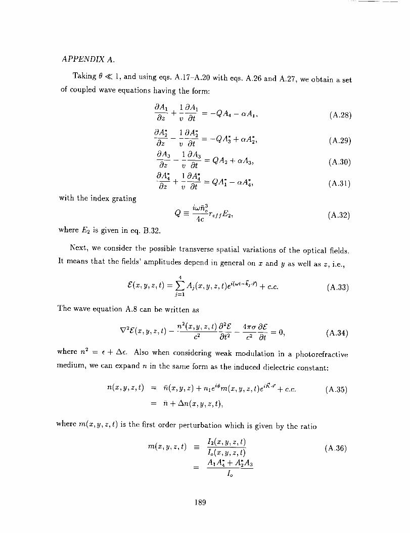
APPENDIX A.
Taking 0 << 1, and using eqs. A.17-A.20 with eqs. A.26 and A.27, we obtain a set
of coupled wave equations having the form:
OA1 10A1
0-----_+ - QA4 - aA1, (A.28)v Ot
with the index grating
OA_ 1 OA_Oz v Ot - QA; + o_A_, (A.29)
OA3 10A3
Oz v Ot - QA2 + o_A3, (A.30)
OA"4 I OA*4O---Z+ -QA_-aA_, (A.31)v Ot
where E_ is given in eq. B.32.
Q - iwfi 34c reyyE2' (A.32)
Next, we consider the possible transverse spatial variations of the optical fields.
It means that the fields' amplitudes depend in general on z and Y as well as z, i.e.,
4
£(z,y,z,t) = y_ Aj(z,y,z,t)ei("-k','_ + c.c. (A.33)j=l
The wave equation A.8 can be written as
V2S(x,y,z,t)_ n2(x,y,z,t) 02$ 4zcaO£c 2 Ot 2 c 2 Ot - O, (A.34)
where n 2 = e + Ae. Also when considering weak modulation in a photorefractive
medium, we can expand n in the same form as the induced dielectric constant:
n(x,y,z,t) = + + c.c.
= fi+An(x,y,z,t),
(A.35)
where rn(x, y, z, t) is the first order perturbation which is given by the ratio
Is(x, y, z, t)
rn(z,y,z,t) =_ Io(z,y,z,t) (A.36)
A1A_ + A_A3
Io
189
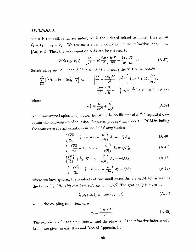
APPENDIX A.
and fi is the bulk refractive index, An is the induced refractive index. Here /(_ =-
f_4- /_1 = /_2- k3. We assume a small modulation in the refractive index, i.e.,
JAn I << ft. Then the wave equation A.34 can be reduced to
v E(x,y,z,t) - -j + c2 ] or2 ot - o. (A.37)
Substituting eqs. A.33 and A.35 in eq. A.37 and using the SVEA, we obtain
,=1
c2 -_ + iw A,}e -'k''e + c.c. = 0, (A.38)
where 02 02V_ -= -- + -- (A.39)
Ox 2 Oy _
is the transverse Laplacian operator. Equating the coefficients of e-';_'e separately, we
obtain the following set of equations for waves propagating inside the PCM including
the transverse spatial variations in the fields' amplitudes:
2k + _' " V + a + -_ A1 = -QA4, (A.40)
_ 2___-_-+_:2.V+a+_-_ A;=QA;, (A.41)
2k + t:3" V + a + _ Aa = -QA2, (A.42)
- 2---£-+ ]%. V + a + -_ A*4 = QA_ (A.43)
where we have ignored the products of two small quantities viz nlOAi/Ot as well as
the terms (1/w)OAi/Ot; a = 2_ra/cx/'-_ and v = c/v/_. The grating Q is given by
Q(x,y,z,t) - %m(x,y,z,t), (A.44)
where the coupling coefficient 70 is
- iwnle_¢ (A.45)70 - 2c
The expressions for the amplitude nl and the phase ¢ of the refractive index modu-
lation are given in eqs. B.55 and B.56 of Appendix B.
190

Appendix B
The Kukhtarev equations
In this appendix we use Kukhtarev band transport model [42] to derive the ba-
sic equations governing the hologram formation process in photorefractive media. In
Kukhtarev model, the photorefractive materials are assumed to contain donor and
acceptor traps which arise from the crystals' impurities. These traps introduce inter-
mediate electronic energy states in the bandgap of the insulators. When photons of
sufficient energy are present, electronic transitions by photoexcitation take place. As
a result of the transitions, charge carriers are excited into the conduction band and
the ionized donors become empty trap sites. Furthermore, movements of the charge
carriers are generally described by diffusion, drift and the photovoltaic effect [16].
The migration of the charge carriers from bright regions where they are photoexcited
to dark regions where they are recombined with acceptors builds up a space-charge
field inside the crystal. The space-charge field modulates the material's refractive
index via the linear electrooptic effect [40] (Pockel effect).
The space-charge field created by the migration and trapping of the charge carriers
is determined by the following set of transport equations:
On _ ON + 1V. 5' (continuity) (B.1)Ot Ot q
Ot - (SI +/3)(ND -- N +) -_/RnN + (rate equation), (B.2)
191

APPENDIX B.
-f = q#nE, - kBT#Vn + pI_c (current equation), (B.3)
V./_ = q (n + NA - N +) (Poisson's law), (B.4)
where (SI +/3)(ND--N +) is the rate of charge carrier generation, 7RnN+D is the rate of
trap capture. Here S is the cross-section of photoionization,/3 is the rate of thermal
generation, "_R is the carrier-ionized trap recombination rate coefficient and n and
N + are the concentrations of the carriers and ionized traps, ND is the concentration
of the donor traps, I is the light intensity, NA is the acceptor concentration, # is
the mobility, T is the temperature, kB is the Boltzman constant, e is the dielectric
constant, pI is the photovoltaic current and p is the photovoltaic constant, _c is the
unit vector along the c axis of the crystal, /_ is the total field which includes the
induced space-charge field /_ and any external or internal fields such as internal
ferroelectric fields; and q is the charge of the charge carrier.
In general # and e are tensors and ND and NA could vary with position. For
simplicity we will assume that # and e are scalars and No and NA are constant
throughout the material. Eqs. B.I-B.4 are nonlinearly coupled and generally difficult
to solve without some approximations. In the following we will simplify the band
transport equations using various approximations to solve for the space-charge field
and obtain the basic equation that governs it.
We begin with a perturbation scheme to linearize the above coupled equations.
To this end, we let (see figure B.1)
I(x,z,t) = Io(z,t) + [h(z,t)e -ig'_ + c.c.] (B.5)
E(x,z,t) = Eo(z,t) + [E_(z,t)e -'K,': + c.c.] , (B.6)
= no(Z,t)+ [n (z,t)S + cc], (BT)
= N o(z,t) + + c.c.], (BS)
j(x,z,t) = jo(z,t) + [j2(z,t)e -iKx': + c.c.] . (B.9)
Here E(x, z, t) is the overall electric field in the photorefractive material, which is the
sum of any external field Eo and the induced space-charge field E2, and we assume
192
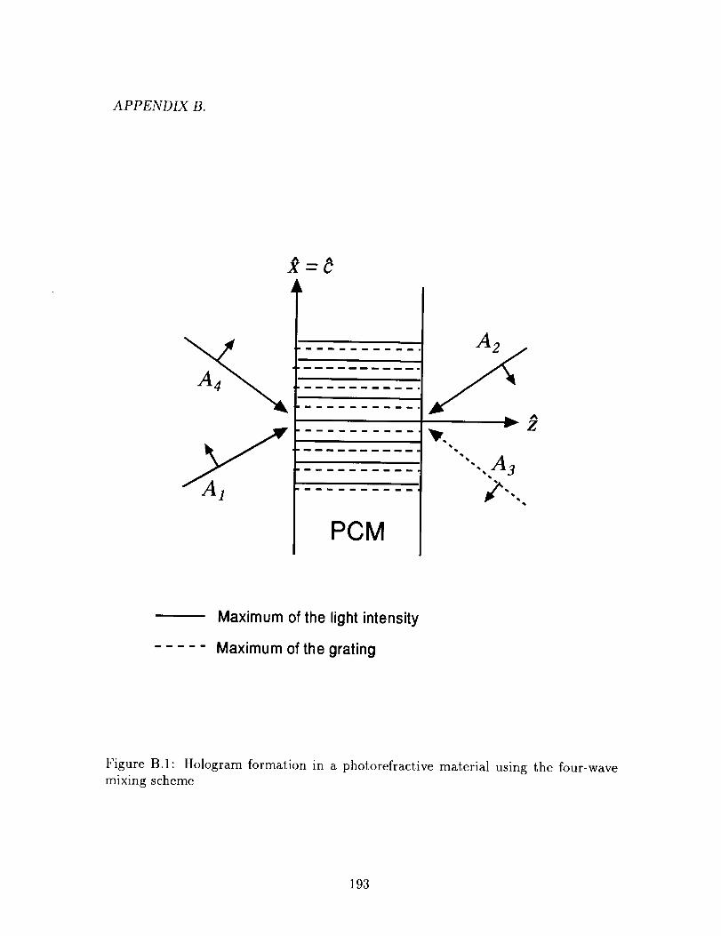
APPENDIX B.
A2
""',A3
PCM
Z
Maximum of the light intensity
Maximum of the grating
Figure B.I: Hologram formation in a photorefractive material using the four-wavemixing scheme
193
APPEND_ B.
that I2(z, t) varies relatively slowly along the z-axis as compared to the fast change
of e -at'_x along the x-axis, etc. (SVEA).
At first we consider the quasi-steady static case, i.e. Ono/Ot _ ON+o/Ot _ O. We
also assume that there are a lot of available donors and acceptors to linearize the
generation and recombination rates, i,e., ND >> ND -- N + and NA >> n. From now
on, we also ignore the small thermal factor, i.e. _ << SI. Then, from eq. B.4 and
assuming the SVEA, we have
OEsc _ q-(n + NA- N+). (B.10)C_X -- (.
We obtain the following equations upon equating the zeroth order terms and the
coefficients of e-iK_z:
lX x£
N+o = NA + no _ NA, (B.11)
(B.12)
Consider a maximum space-charge field with charge separation comparable to the
grating period such that
K::E;- qNn (B.13)£
Then, in eq. B.12i<
E: = _--;(n_- N_+_). (B.14)
Now, from eq. B.2, we have
ON+2 -iKxx Jr- C.C.]S [Io + I2e -iK_ + c.c.] ND (B.15)
" " hf+ _-iKxx C.C.] ,+ + + +
which gives us
and
S IoND ,,_ _SI°ND (B.16)no 7RN+ ° "/RNA
- SI2ND -%[n2N+o + noN_2]. (B.17)
194

APPENDIX B.
For the quasi-steady state, or when the generation rate equals the recombination rate,
i.e. ON+2/Ot _ O, we have
N+ _ _ SI2ND"/nno
Combinding eqs. B.1 and B.3, we get
Ot + c.c.
NA
n o
n2. (B.18)
r+ 1D_2e-iK_z + c.c.t
--_ [no + n2e -iK,x + c.c.] [(-iI(x)E2e -iK*x + c.c.J
-# (-iI(x)n2e -iJ'_ + c.c.] [Eo + E2e -it<'_ + c.c.]
kBT# c.c.]+_ [(-iI(x)_-iK_ x +q
P [(-iK.)I2e -i_'=_ + c.c.] .q
(B.19)
As On2/Ot - ON+2/Ot ,,_ 0, we get
(ikBTI(_) [ pIo (I_)]Eo + n2 = -- E2 + -- no. (B.20)q q#no
We recognize the diffusion field ED =-- kBTK_/q and the photovoltaic field Ep _=
pIo/q#no. Then we rewrite n2 as
E2 + Ep I2 / Io
n2 = Eo + iED no. (B.21)
Now, substituting eqs. B.18 and B.21 in eq. B.14, we have the following static space-
charge field:
E#:-iE;(NA+n°)[E +EpI /I°v)V-; t ;4/-27 +TooI2] (B.22)Since
(NA + _o) qNA q(ND- NA) qN_E; No . " eI(-----__ eI'(_ND NA =-- eI(_ -- Eq, (B.23)
where N_ is the effective trap density, we can simplify eq. B.22 such that the modu-
lation of the static space-charge field is
[(Eo + Ep) + iEu] I2E s : -iEq [_o__-i-_q + Eo)] (_)" (B.24)
195
APPENDIX B.
Next, we examine the time development of the space-charge field. In the short
writing time limit, i.e. shortly after illumination, N + will not change greatly from its
dark values (i.e. N + _ NA). Then eq. B.2 may be written as
ON+ - SI(ND - NA) -- n__ (B.25)Ot rR '
with rR = 1/%NA. Substituting this in eq. B.1,
On _ SI(ND - NA) -- n___ (B.26)Ot ra
Ox #nEst q Ox + I .
As we expect On�Or = O(n/rn,), whereas rd, is the dielectric relaxation time, for
illluminating times greater than a few rR we can then make the approximation that
rROn/Ot _ O. Also, for times short compared to rd., the space-charge field will not
change greatly and we may make the further approximation Esc _ Eo. Then eq. B.26
will reduce to
0 ,,_ rRS [Io + I2e -'K_ + c.c.] (No - NA)- (B.27)
k,T# O2n p [012 e_iKx_ + c.c.] ,q Ox 2 q J
which, after equating the coefficients of e -ig_x, gives
1 + iEv/E.M "no (12) (8.28)n2 = + ED/DM -- zEo/EM _o
EM + iEv .] (Is)= (EM+ED)-iEo no _ ,
with EM =-- 1/(graK_:). In eq. B.24, as N + ",_ NA, then we have for short time
N_ _ NA_{_ (_IND-- _-_R) t . (8.29)
So, from eq. B.4, and with NA, No - NA 2>>n , we have
OEs_ -q-(_-SIND) t'Oxe
which gives, by equating the coefficients of e -iKxx,
iq SI2 ND)E2 _ e--[_: ( _ - t.
(B.30)
(B.31)
196
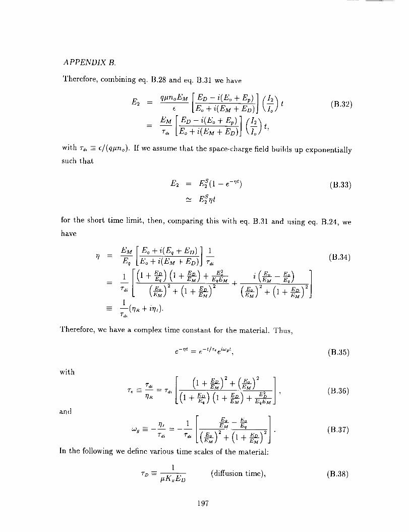
APPENDIX B.
Therefore, combining eq. B.28 and eq. B.31 we have
[Eo-+-i(--E-£M + ED)J _ t (B.32)
EM [ ED -- i(Eo + Ep) 12
with rd, = e/(q#no). If we assume that the space-charge field builds up exponentially
such that
E2 : Es(1 - e -'')
_'_ ESqt
(B.33)
for the short time limit, then, comparing this with eq. B.31 and using eq. B.24, we
have
EM[ Eo+ i(Eq+ ED)] 1 (B.34)
1
Td,
1
Tdi
u_a(1 + Eq)(1 + EM) + EqEM +
Eo) 2 + (1 + E_r_)2EM ] EM ]
- --(rlR+irl, ).
E¢_ kE_ _
AV EM ] .]
Therefore, we have a complex time constant for the material. Thus,
e-_ t _ e-t/reeiw9 t, (B.35)
with
and
Te_
rdi (I + EM] )__-- Td i ------ ^
_E_zzqR 1 + Eq)(1 -4- EE--_-_] +
M ] q M .J
_ Eo
_ q_ 1 E M -- Eq
O.)g __
Td, r_, (E_)2 + (I+EM___)2
In the following we define various time scales of the material:
(B.36)
(B.37)
1
TD =---#K_ED (diffusion time), (B.38)
197
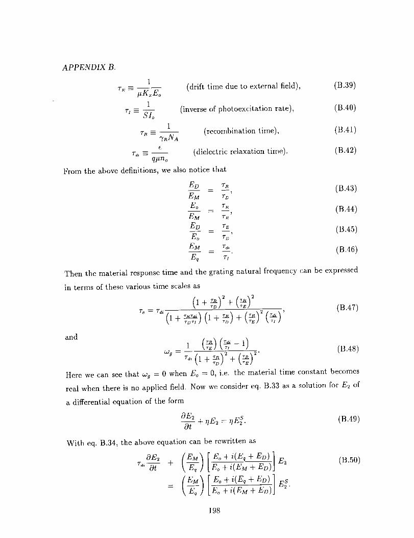
APPENDIX B.
7E - _KxEo
TIc--
Tu,--
q#no
From the above definitions, we also notice that
(drift time due to external field),
(inverse of photoexcitation rate),
(recombination time),
(dielectric relaxation time).
ED "rn
E M 7"D
Eo T R
)
EM TE
ED TE
Eo TD
EM T_i
(B.39)
(B.40)
(B.41)
(B.42)
(B.43)
(B.44)
(B.45)
(B.46)Eq TI
Then the material response time and the grating natural frequency can be expressed
in terms of these various time scales as
(1+ +•v, "_ (B.47)
"re = Tdi 2
(1 + T_TTTTTTTT_TD're" (1-4-"D) + ('r_) (¢'-_/)
and
1 (,_)(,_-_,- l) (B.48)COg _ 2"
Here we can see that COg= 0 when Eo = 0, i.e. the material time constant becomes
real when there is no applied field. Now we consider eq. B.33 as a solution for E2 of
a differential equation of the form
OE___!+ tiE2 = tiE s. (B.49)Ot
With eq. B.34, the above equation can be rewritten as
OE2 (EM) [ Eo + i(Eq + ED)
1E s
(B.50)
198
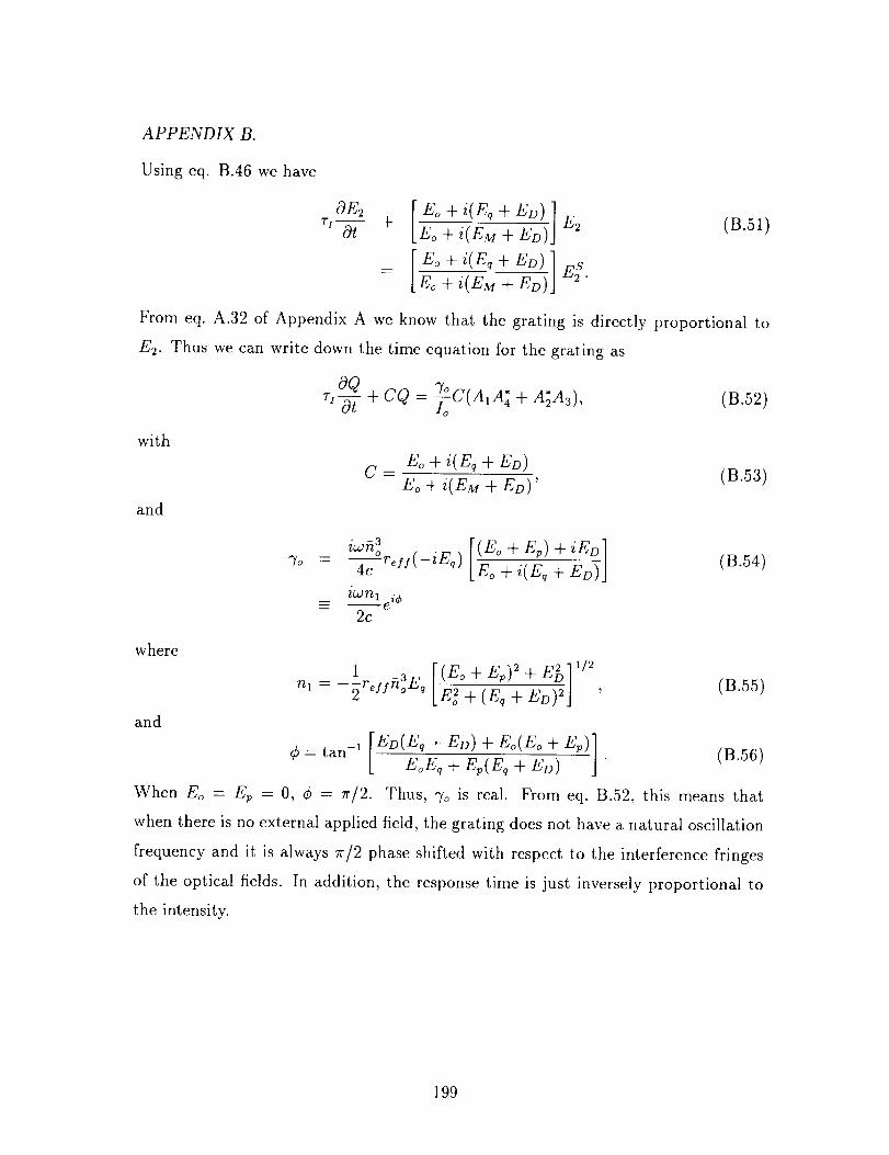
APPENDIX B.
Using eq. B.46 we have
oF, [Eo+/(E,+E.)]r,--_-- + [_i-_M_-_-D)jE2 (B.51)
= [_oo__i-_M-+_-)jE s.
From eq. A.32 of Appendix A we know that the grating is directly proportional to
E2. Thus we can write down the time equation for the grating as
OQ % . .-_,-g?+ CQ : _C(AIA4 + A2A3), (B.52)
with
and
Eo + i(Eq + ED)
c = Eo+ i(EM + El))' (B.53)
iwfi 3 [(Eo + Ep) + iED]% - 4c r_]f(-iEq) [E _ i_q _ E--_D)] (B.54)
iCOT/1-- ei¢
2c
where
and
1 3 [(EoArEp)2ArE )]1/2 (B.55)
¢ = tan- 1 El)(Eq + ED) + Eo(Eo + Ep)] (B.56)Eo Eq + Ep (Eq + ED) ]
When Eo = E v = 0, ¢ = 7r/2. Thus, 70 is real. From eq. B.52, this means that
when there is no external applied field, the grating does not have a natural oscillation
frequency and it is always 7r/2 phase shifted with respect to the interference fringes
of the optical fields. In addition, the response time is just inversely proportional to
the intensity.
199
REFERENCES
[1] J. N. Cederquist, "Optical Feedback Processing," in Optical Signal Processing,
(J. L. Horner, ed.), London: Academic Press, 1983.
[2] P. De Santis, F. Gori, G. Guttari, and C. Palma, "Optical systems with feed-
back," Optica acta, 23, pp. 505-518, 1976.
[3] R. J. Marks, "Coherent optical extrapolation of 2-D band-limited signals: pro-
cessor theory," Appl. Opt., 19, pp. 1670-1672, 1980.
[4] T. W. Hansch, F. Varsanyi, and A. L. Schawlow, "Image amplification by dye
lasers," Appl. Phys. Left., 18, pp. 108-110, 1971.
[5] R. P. Akins and S. H. Lee, "Two-stage injection-locked ring dye laser/amplifier
for coherent image amplification," J. Opt. Soc. Am., A 7, pp. 533-538, 1984.
[6] P. Pellat-Finet and J. L. De Bougrenet De La Tocnaye, "Optical generator of
spheroidal wave functions, using a BSO crystal," Opt. Commun., 55, pp. 305-
310, 1985.
[7] Y. Fainman, E. Klancnik, and S. H. Lee, "Optimal coherent image amplification
by two-wave coupling in photorefractive BaTiO3," Opt. Eng., 25, pp. 228-234,
1986.
[8] J. Feinberg and R. W. Hellwarth, "Phase conjugating mirror with continuous
wave gain," Opt. Left., 5, pp. 519-521, 1980.
[9] B. H. Softer, G. J. Dunning, Y. Owechko, and E. Marom, "Associative holo-
graphic memory with feedback using phase-conjugate mirrors," Opt. Lett., 11,
pp. 118-120, 1986.
[10] D. Z. Anderson, "Coherent optical eigenstate memory," Opt. Left., 11, pp. 56-
58, 1986.
[11] A. Yariv and S. K. Kwong, "Associative memories based on message-bearing
optical modes in phase-conjugate resonators," Opt. Left., 11, pp. 186-188, 1986.
200
REFERENCES
[12] T. Kohonen, Self organization and associative memory. Springer-Verlag, 1984.
[13] J. J. Hopfield, "Neural networks and physical systems with emergent collective
computational abilities," Proc. Nat. Acad. Sci., 79, pp. 2554-2562, 1982.
[14] N. H. Farhat and D. Psaltis, "Optical implementation of associative memory
based on models of neural networks," in Optical Signal Processing, (J. L. Horner,
ed.), London: Academic Press, 1983.
[15] T. J. Hall, R. Jaura, L. M. Connors, and P. D. Foote, "The photorefractive
effect -A review," Prog. Quant. Electr., 10, pp. 77-146, 1985.
[16] P. Giinter and J. P. Huignard, Photorefractive Materials and Their Applications
I _ II. Springer-Verlag, 1988.
[17] J. M. Heaton and L. Solymar, "Transient energy transfer during hologram for-
mation in photorefractive crystals," Optica Acta, 32, pp. 397-408, 1985.
[18] G. C. Papen, B. E. A. Saleh, and J. A. Tataronis, "Analysis of transient phase
conjugation in photorefractive meida," J. Opt. Soc. Am., B 5, pp. 1763-1774,
1988.
[19] W. Krolikowski, K. D. Shaw, M. Cronin-Golomb, and A. Bledowski, "Stability
analysis in photorefractive crystals," J. Opt. Soc. Am., B 6, pp. 1828-1833,
1989.
[20] P. Giinter, E. Volt, M. Z. Zha, and J. Albers, "Self-pulsation and optical chaos in
self-pumped photorefractive BaTiO3," Opt. Commun., 55, pp. 210-214, 1985.
[21] A. M. C. Smout and R. W. Eason, "Regular oscillations and self-pulsating in
self-pumped BaTiO3," Opt. Commun., 59, pp. 77-82, 1986.
[22] D. J. Gauthier, D. Narum, and R. W. Boyd, "Observation of deterministic
chaos in a phase conjugate mirror," Phys. Rev. Lett., 58, pp. 1640-1643, 1987.
[23] J. P. Jiang and J. Feinberg, "Dancing modes and frequency shifts in a phase
conjugator," Opt. Lett., 12, pp. 48-50, 1987.
[24] W. Krolikowski, B. S. Chen, and M. Cronin-Golomb, "Temporal instabilities in
an externally driven ring phase conjugator," J. Opt. Soc. Am., B 8, pp. 1455-
1460, 1991.
[25] G. Hussain, S. W. James, and R. W. Eason, "Observation and Modeling of
dynamic instabilities in the mutually pumped bird-wing phase conjugator in
BaTiO3," J. Opt. Soc. Am., B 7, pp. 2294-2298, 1990.
201
REFERENCES
[26]
[27]
[28]
[29]
[3o]
[31]
[32]
[33]
[34]
[35]
[36]
[37]
[38]
D. Wang, Z. Zhang, X. Wu, and P. Ye, "Instabilities in a mutually pumped
phase conjugator of BaTiOa," J. Opt. Soc. Am., B 7, pp. 2289-2293, 1990.
G. Valley and G. Dunning, "Observation of optical chaos in a phase conjugate
resonator," Opt. Lett., 9, pp. 513-515, 1984.
J. L. Bougrenet, P. Pellat-Finet, and J. P. Huignard, "Effect of using a Bl_SiO2o
light amplifier on the formation and competition of modes in optical resonators,"
J. Opt. Soc. Am., B 3, pp. 315-319, 1986.
A. Bledowski, W. Krolikowski, and A. Kujawski, "Temporal instabilities in
single photorefractive four-wave mixing," J. Opt. Soc. Am., B 6, pp. 1544-
1547, 1989.
K. D. Shaw and M. Cronin-Golomb, "Stability of multiple solutions in pho-
torefractive four-wave mixing with external electric field," Opt. Cornmun., 76,
pp. 151-156, 1990.
W. Krolikowski, M. R. Belic, M. Cronin-Golomb, and A. Bledowski, "Chaos in
photorefractive four-wave mixing with a single grating and a single interaction
region," J. Opt. Soc. Am., B 7, pp. 1204 1209, 1990.
M. R. Belic, D. Timotijevic, and W. Krolikowski, "Multigrating phase conju-
gation:chaotic results," J. Opt. Soc. Am., B 8, pp. 1723-1731, 1991.
M. Horowitz, D. Kligler, and B. Fischer, "Time-dependent behavior of pho-
torefractive two and four-wave mixing," J. Opt. Soc. Am., B 8, pp. 2204-2217,
1991.
S. R. Liu and G. Indebetouw, "Dynamics of a phase conjugate resonator: tran-
sient buildup and decay rates," Appl. Phys. B, 54, pp. 247-258, 1992.
L. K. Dai, Y. S. Gou, C. Gu, and P. Yeh, "Instabilities in coupled photorefractive
ring cavities and self-pumped phase conjuators: I & II," Appl. Phys. B, 54,
pp. 57-70,156-166, 1992.
H. Kogelnik, "Coupled wave theory for thick hologram gratings," Bell Syst.
Tech. J., 48, pp. 2909-2947, 1969.
V. V. Eliseev, V. T. Tikhonchuk, and A. A. Zozulya, "One-mirror self-pumped
phase conjugator: three-dimensional analysis," Opt. Commun., 85, pp. 520-
526, 1991.
W. Krolikowski and M. Cronin-Golomb, "Photorefractive wave mixing with
finite beams," Opt. Comraun., 89, pp. 88-98, 1992.
202

REFERENCES
[39] "Transverse effects in nonlinear optical systems", J. Opt. Soc. Am. B 7, Special
issues (June and July, 1990).
[40] A. Yariv, Optical electronics. Holt, Rinehart and Winston, Inc., 1985.
[41] N. V. Kukhtarev, V. B. Markov, and S. G. Odulov, "Transient energy transfer
during hologram formation in LiNbO3 in external electric field," Opt. Commun.,
23, pp. 338-343, 1977.
[42] N. V. Kukhtarev, V. B. Markov, S. G. Odulov, M. S. Soskin, and V. L. Vinet-
skii, "Holographic storage in electro-optic crystals. II. Beam coupling - light
amplification," Ferroelectrics, 22, pp. 961-964, 1979.
[43] V. L. Vinetskii, N. V. Kukhtarev, S. G. Odulov, and M. S. Soskin, "Dynamic
self-diffraction of coherent light beams," Soy. Phys. Usp, 22, pp. 742 756, 1979.
[44] tI. Kogelnik, "Holographic image projection through imhomogeneous media,"
Bell Syst. Tech. J., 44, pp. 2451-2455, 1965.
[45] A. E. Siegman, P. A. Belanger, and A. Hardy, "Optical resonators using phase-
conjugate mirrors," in Optical Phase Conjugation, (R. Fisher, ed.), pp. 465-535,
Academic Press, New York, 1983.
[46] K. P. Lo and G. Indebetouw, "Iterative image processing using a cavity with a
phase conjugate mirror," Appl. Opt., 31, pp. 1745-1753, 1992.
[47] M. F. Barsky, Holographic sensing for control of flexible structures. PhD thesis,
Electrical Engineering, Virginia Polytectnic Institute & State University, 1990.
[48] P. D. Drummond and A. T. Friberg, "Specular reflection cancellation in an
interferometer with a phase-conjugate mirror," J. Appl. Phys., 54, pp. 5618
5625, 1983.
[49] A. T. Friberg, M. Kauranen, and R. Salomaa, "Dynamics of Fabry-Perot res-
onators with a phase-conjugate mirror," J. Opt. Soc. Am., B 3, pp. 1656 1672,
1986.
[50] M. Cronin-Golomb, F. Baruch, S. K. Kwong, J. O. White, and A. Yariv, "Non-
degenerate optical oscillation in a resonator formed by two phase-conjugate
mirrors," Opt. Lett., 10, pp. 353-355, 1985.
[51] S. S. Lafleur and R. C. Montgomery, "Real-time dynamic holographic image
storage device," Appl. Opt., 29, p. p.3976, 1990. U.S. patent 4,913,534.
[52] A. M. Glass, D. Von der Linde, and T. D. Negran, "High-voltage bulk pho-
tovoltaic effect and the photorefractive process in LiNbOa," Appl. Phys. Lett.,
25, pp. 233-235, 1974.
203

REFERENCES
[53]
[54]
[55]
G. C. Valley and M. B. Klein, "Optimal properties of photorefractive materials
for optical data processing," Opt. Eng., 22, pp. 704-711, 1983.
G. A. Brost and R. A. Motes, "Origin of the sublinear photorefractive response
time in BaTiO3," Opt. Lett., 15, pp. 1194-1196, 1990.
V. Kalinin and L. Solymar, "Transient effects in four-wave mixing in photore-
fractive passive phase conjugate mirrors," Applied Physics, B 45, pp. 129-135,1988.
[56]
[57]
N. B. Abraham, A. M. Albano, and N. B. Tufillaro, "Complexity and chaos,"
in Measures of Complexity and Chaos, (Abraham, N.B. et als, ed.), pp. 1-27,
Plenum Press, New York, 1990.
F. C. Moon, Chaotic Vibrations: An introduction for applied scientists and
engineers. N.Y., N.Y.: Wiley, 1987.
[58]
[59]
[6O]
[61]
[62]
E. N. Lorenz, "Deterministic nonperiodic flow," J. Atmos. Sci., 20, pp. 130-
144, 1963.
C. Corduneanu, Almost Periodic Functions. Interscience Publishers, N.Y., 1968.
P. Berge, Y. Pomeau, and C. Vidal, Order within Chaos. John Wiley and Sons,
New York, 1984.
S. N. Rasband, Chaotic dynamics of nonlinear systems. Wiley, 1990.
G. L. Baker and J. P. Gollub, Chaotic dynamics: an introduction. Cambridge
Univ. Press, 1990.
[63]
[64]
[65]
P. Grassberger and I. Procaccia, "Estimation of the Kolomogrov entropy from
a chaotic signal," Phys. Rev. A, 28, pp. 2591-2593, 1983.
F. Takens, "Detecting strange attractors in turbulence," in Dynamical sys-
tems and Turbulence, 898 of Lecturer Notes in Mathematics, (Rand, D. A.
and Young, L-S, ed.), pp. 366-381, Berlin: Springer-Verlag, 1981.
G. Nicolis and I. Prigogine, Self-organization in nonequilibrium systems. New
York: Wiley, 1977.
[66] S. Chandrasekhar, Hydrodynamic and hydromagnetic stability. Clarendon Press,1961.
[67] A. Libchaber and J. Maurer, "A Rayleigh-Benard experiment: helium in a small
box," in Nonlinear phenomena at phase transitions and instabilities, (Riste, T.,
ed.), pp. 259-86, Plenum Press, New York, 1982.
204
REFERENCES
[68] P. Manneville, Dissipative structures and weak turbulence. San Dieao, CA: Appl.
Phys., 1990.
[69] T. B. Benjamin and J. E. Feir, "The disintegration of wavetrains on deep water,"
J. Fluid Mech., 27, pp. 417-430, 1967.
[7o] L. A. Lugiato, C. Oldano, and L. M. Narducci, "Cooperative frequency locking
and stationary spatial structures in lasers," J. Opt. Soc. Am., B 5, pp. 879-888,
1988.
[71] L. A. Lugiato, G. L. Oppo, M. A. Pernigo, J. R. Tredicce, L. M. Narducci, and
D. K. Bandy, "Spontaneous spatial pattern formation in lasers and cooperative
frequency locking," Opt. Commun., 68, pp. 63-68, 1988.
[72] L. A. Lugiato, F. Frati, L. M. Narducci, P. Ru, J. R. Tredicce, and D. K. Bandy,
"Role of transverse effects in laser instabilities," Phys. Rev. A, 37, pp. 3847-
3866, 1988.
[73] L. A. Lugiato, F. Frati, L. M. Narducci, and G. L. Oppo, "Spontaneous breaking
of the cylindrical symmetry in lasers," Opt. Commun., 69, pp. 387-392, 1989.
[74] L. A. Lugiato, G. L. Oppo, J. R. Tredicce, and L. M. Narducci, "Instabilities
and spatial complexity in a laser," J. Opt. Soc. Am., B 7, pp. 1019-1033, 1990.
[75] G. D'Alessandro and G. L. Oppo, "Gauss-Laguerre modes: a "sensible" basis
for laser dynamics," Opt. Commun., 88, pp. 130-136, 1992.
[76] M. Brambilla, F. Battipede, L. A. Lugiato, V. Penna, F. Prati, C. Tamm, and
C. O. Weiss, "Transverse laser patterns. I. Phase singularity crystals," Phys.
Rev. A, 43, pp. 5090-5113, 1991.
[77] M. Brambilla, F. Battipede, L. A. Lugiato, V. Penna, F. Prati, C. Tamm, and
C. O. Weiss, "Transverse laser patterns. II. Variational principle for pattern
selection, spatial multistability and laser hydrodynamics," Phys. Rev. A, 43,
pp. 5113-5120, 1991.
[78] P. Coullet, L. Gil, and F. Rocca, "Optical vortices," Opt. Commun., 73,
pp. 403-407, 1989.
[79] P. Coullet and J. Lega, "Defect-mediated turbulence in wave patterns," Euro-
phys. Letters, 7, pp. 511-516, 1988.
[80] P. Coullet, L. Gil, and J. Lega, "Defect-mediated turbulence," Phys. Rev. Lett.,
62, pp. 1619-1622, 1989.
[81] Balian, R. et al, ed., Physics of defects, (Amsterdam), North-Holland, 1981.
2O5

REFERENCES
[82]
[83]
[84]
W. A. Burke, ed., Theory of self-reproducing automatoa. University of Illinois
Press, 1966.
K. Kaneko, "Transition from torus to chaos accompanied by frequency lookings
with symmetry breaking," Prog. Theor. Phys., 69, pp. 1427-1442, 1983.
K. Kaneko, "Towards thermodynamics of spatiotemporal chaos," Prog. Theoret.
Phys. Suppl., 99, pp. 262-287, 1989.
[85] P. Procaccia, "Weak turbulence and dynamics of topological defects," in Mea-
sures of Complexity and Chaos, (Abraham, N.B. et als, ed.), Plenum Press,
New York, 1990.
[86] F. T. Arecchi, G. Giacomelli, P. L. Ramazza, and S. Residori, "Vortices and de-
fect statistics in two-dimensional optical chaos," Phys. Rev. Lett., 67, pp. 3749-
3752, 1991.
[87]
[88]
[89]
[9o]
[91]
[92]
[93]
[94]
[95]
G. Indebetouw and S. R. Liu, "Defect-mediated spatial complexity and chaos
in a phase-conjugate resonator," Opt. Commun., 91, pp. 321-330, 1992.
S. R. Liu and G. Indebetouw, "Periodic and chaotic spatiotemporal states in
a phase-conjugate resonator using a photorefractive BaTiO3 phase-conjugate
mirror," J. Opt. Soc. Am., B 9, pp. 1507-1520, 1992.
M. Berry, "Singularities in waves and rays," in Physics of defects, (Balian, R.
et als, ed.), (Amsterdam), pp. 455-543, North-Holland, 1981.
J. F. Nye and M. V. Berry, "Dislocations in wavetrains," Proc. Roy. Soc. Lond.,
336, pp. 156-190, 1974.
N. B. Baranova, A. V. Mamaev, N. F. Pilipetsky, V. V. Shkunov, and B. Y. Zel-
dovich, "Wave-front dislocations: topological limitations for adaptive systems
with phase conjugation," J. Opt. Soc. Am., B 5, pp. 525-528, 1983.
J. Nye, "Dislocations and disclinations in transverse electromagnetic waves,"
in Physics of defects, (Balian, R. et. al, ed.), pp. 122-155, North Holland,
Amsterdam, 1981.
F. J. Wright, "Wavefront dislocations and their analysis using catastrophe
theory," in Structural stability in Physics, pp. 141-156, Heidelberg: Springer-
Verlag, 1979.
Laser. University Science Book, Mill Valey, 1986.
A. Brandstater and H. L. Swinney, "Strange attractors in weakly turbulent
Couette-Taylor flow," Phys. Rev. A, 35, pp. 2207-2220, 1987.
206
REFERENCES
[96]
[97]
P. Grassberger and I. Procaccia, "Characterization of strange attractors," Phys.
Rev. Left., 50, pp. 346-349, 1983.
P. Coullet, "Defect-induced spatio-temporal chaos," in Measures of Complexity
and Chaos, (Abraham, N.B. et als, ed.), (N. Y.), pp. 367 373, Plenum Press,1989.
[98]
[99]
G. Oppo, M. A. Pernigo, and L. M. Narducci, "Characterization of spatiotem-
poral structures in lasers: A progress report," in Measures of Complexity and
Chaos, (Abraham, N.B. et als, ed.), (N.Y.), pp. 395-404, Plenum Press, 1989.
F. T. Arecchi, G. Giacomelli, P. L. Ramazza, and S. Residori, "Experimental
evidence of chaotic itinerancy and spatiotemporal chaos in optics," Phys. Rev.
Left., 65, pp. 2531-2534, 1990.
[100]
[101]
A. Aceves, H. Adachihara, C. Jones, J. C. Lerman, D. W. McLaughlin,
J. V. Moloney, and A. C. Newell, "Chaos and coherent structures in partial
differential equations," Physica D, 18, pp. 85-112, 1986.
C. O. Weiss and R. Vilaseca, Dynamics of lasers. VCH Pulbisher Inc. Weinheim,1991.
[102] J. P. Crutchfield and K. Kaneko, "Phenomenology of spatio-temporal chaos," in
Directions in chaos, (B. L. Hao, ed.), pp. 272-353, World Scientific, Singapore,1987.
[103]
[104]
[105]
V. L. Vinetskii, N. V. Kukhtarev, S. G. Odulov, and M. S. Soskin, "Dynamic
self-diffraction of coherent light beams," Soy. Phys. Usp, 22, pp. 742-756, 1979;
and N. V. Kukhtarev, V. B. Markov, S. G. Odulov, M. S. Soskin, and V. L.
vinetskii, "Holographic storage in electro-optic crystal. II. Beam coupling-light-
amplication," Ferroelectrics, 22, pp. 961-964, 1979.
J. Goodman, Introduction to Fourier Optics. McGraw-Hill, 1968.
G. Reiner, P. Meystre and E. M. Wright, "Transverse dynamics of a phase-
conjugate resonator," J. Opt. Soc. Am. B 4, pp. 675-686, 1987 and J. Opt.
Soc. Am. B 4, pp. 865 874, 1987; G. Reiner, M. R. Belic and P. Meystre,
"Optical turbulence in phase-conjugate resonators," J. Opt. Soc. Am B 5, pp.
1193-1210, 1988.
[106] A. C. Newell, "The dynamics of patterns: A survey," in Propagation in systems
far from equilibrium, (J. W. Wesfried et. als., ed.), pp. 122 155, Springer-Verlag,
Berlin, 1988.
[107] G. J. Dunning, "Improved spatial and temporal performance of a phase con-
jugate resonator by using an intracavity fiber optic taper", (Presented at OSA
Annual Meeting, Albuquerque, NM 1992).
207

REFERENCES
[108] M. Brambilla, L. A. Lugiato, M. V. Pinna, F. Prati, P. Pagani, P. Vanotti,
M. Y. Li, and C. O. Weiss, "The laser as nonlinear element for an optical
associative memory," Opt. Commun., 92, pp. 145-164, 1992.
208

Form ApprovedREPORT DOCUMENTATION PAGE OMBNo. 0704-0188
Public rlll;_r_ng burden Ic¢ thB collectionol inforrnallonis estimated to average 1 hour per rl_oonm, indudit_l the Ul'fmIGr _ Irtlltrtctlonl. _ I=iltlng _ IOUrC_..galhertng and tnalntalnmg the data needed, and cotrOlet+ngand reviewing Iha collect=onOfreformation. SorKI¢otntrl_,tll re_a_dtngIhls burd4mimtlmall ot mty otha alplK= Of thillcollectiot_o( intorm_fion,including sug_esl_ns Io( reducingthis burden, to Washington I.-leadquanerl.Setvcml, Diteclorala for Irtlotmmk)nOperalione acid _. 1215 Jotlerllo_ Cl_Highway. Sude 1204. Adinglon, VA 22202-4302. and to the Office of Management and Budgel. P_ Reduclion Projecl (0704-01M), Washington, DC 20503.
1. AGENCY USE ONLY (Leave blank) 2. REPORT DATE 3, REPORT TYPE AND DATES COVERED
December 1993 Contractor Report4. TITLE AND SUBTITLE S. FUNDING NUMBERS
Spatiotemporal Behavior and Nonlinear Dynamics in a Phase Conjugate G NAG1-1363Resonator
6. AUTHOR(S)
Siuying Raymond Liu
7. PERFORMING ORGANIZATION NAME(S) AND ADDRESS(ES)
Virginia Polytechnic Institute and State UniversityPhysics Department
Blacksburg, Virginia 24061
9. SPONSORING / MONITORING AGENCY NAME(S) AND ADDRESS(ES)
National Aeronautics and Space Administration
Langley Research CenterHampton, VA 23681-0001
WU 233-03-01-01
8. PERFORMING ORGANIZATIONREPORT NUMBER
10. SPONSORING / MONITORINGAGENCY REPORT NUMBER
NASA CR-4567
11. SUPPLEMENTARYNOTESLangley Technical Monitor: Sharon S. Welch
Dissertation submitted in partial fulfillment of the requirements for the Degree of Doctor of Philosophy in Physics,Virginia Polytechnic Institute and State University, Blacksburg, Virginia, April 1993.
12a. DISTRIBUTION/ AVAILABILITYSTATEMENT
Unclassified-Unlimited
Subject Category 74
12b. DISTRIBUTION COOE
13. ABSTRACT (Maximum 200 words)
The work described in this report can be divided into two parts. The first part is an investigation of the transient behavior andstability property of a phase conjugate resonator (PCR) below threshold. The second part is an experimental and theoreticalstudy of the PCR's spatiotemporal dynamics above threshold.
The time-dependent coupled wave equations for four-wave mixing (FWM) in a photorefractive crystal, with two distinctinteraction regions caused by feedback from an ordinary mirror, was used to model the transient dynamics of a PCR belowthreshold. The conditions for self-oscillation were determined and the solutions were used to define the PCR's transfer
function and analyze its stability. Experimental results for the buildup and decay times confirmed qualitatively the predictedbehavior.
Experiments were carried out above threshold to study the spatiotemporal dynamics of the PCR as a function of Braggdetuning and the resonator's Fresnel number. The existence of optical vortices in the wavefront were identified by opticalinterferometry. It was possible to describe the transverse dynamics and the spatiotemporal instabilities by modeling thethree-dimensional-coupled wave equations in photorefractive FWM using a truncated modal expansion approach.
14. SUBJECTTERMS
Photorefractive, Resonators, Nonlinear optics, Holographic, Phase conjugation,
Nonlinear dynamics
17. SECURITY CLASSIFICATION
OF REPORT
Unclassified
18. SECU RITY CLASSIFICATION
OF THIS PAGE
Unclassified
NSN 7540-01-280-5500
19. SECURITY CLASSIFICATION
OF ABSTRACT
15. NUMBER OFPAGES
228
16. PRICE CODE
All
20. UMITATION OF ABSTRACT
Standard Form 298 (Ray. 2-89)Pmso'#)ed by ANSI Srd. Z39-18298-102