spatio-temporal factors affecting the growth of cultured ... · biofouling studies showed that six...
TRANSCRIPT

This file is part of the following reference:
Lee, Anne Michelle (2010) Spatio-temporal factors
affecting the growth of cultured silver-lip pearl oyster,
Pinctada maxima (Jameson) (Mollusca: Pteriidae) in West
Papua, Indonesia. PhD thesis, James Cook University.
Access to this file is available from:
http://researchonline.jcu.edu.au/19013/
The author has certified to JCU that they have made a reasonable effort to gain
permission and acknowledge the owner of any third party copyright material
included in this document. If you believe that this is not the case, please contact
[email protected] and quote
http://researchonline.jcu.edu.au/19013/
ResearchOnline@JCU

Spatio-temporal factors
affecting the growth of
cultured silver-lip pearl oyster,
Pinctada maxima (Jameson) (Mollusca: Pteriidae)
in West Papua, Indonesia
Thesis submitted by
Anne Michelle LEE, BSc(Monash), MSc(JCU)
in April 2010
for the degree of Doctor of Philosophy
in the School of Marine & Tropical Biology
James Cook University

i
Pinctada maxima oyster
with silver and gold South Sea pearls

ii
Statement of Access
I, the undersigned, the author of this thesis, understand that James Cook University
will make if available for use within the University Library and, by microfilm or other
means, allow access to users in other approved libraries. All users consulting this
thesis will have to the sign the following statement:
In consulting with this thesis I agree not to copy or closely paraphrase it
in whole of in part without the written consent of the author; and to make
proper public written acknowledgement for any assistance which I have
obtained from it.
Beyond this, I do not wish to place any restrictions on access to this thesis.
Anne Michelle Lee Date

iii
Statement of Sources
Declaration
I declare that this thesis is my own work and has not been submitted in any form for
another degree or diploma at any university and institution of tertiary education.
Information derived from the publish or unpublished work of others has been
acknowledged in the text and a list of references given.
Anne Michelle Lee Date

iv
Acknowledgement
I am grateful to Atlas South-Sea Pearls (formerly Atlas Pacific) for making this study
possible through their financial and in-kind contribution, with special thanks to
members of the Board and Dr Joseph Taylor, former CEO of Atlas Pacific.
I would like to acknowledge my supervisor at James Cook University, Professor Paul
Southgate for his continued advice and support throughout this PhD.
I am grateful to the managers and staff of P. T. Cendana Indopearls at Sorong and in
Aljui for their friendship and support during my stay in Indonesia, especially former
managers Dr Jens Knauer, Jan Jorgensen and the Hatchery team with special thanks to
Abraham Umbu Tehu for his invaluable assistance during field sampling. I would like
to acknowledge Max Ammer from Papua-Diving for providing me with maps of the
sampling area and for his continued friendship. I am grateful to Daniel Bradbury for
his assistance in taking videographs of oyster for me.
At James Cook University, I would like to acknowledge Dr Ashley Williams and
Professor Gary Russ for kindly providing me with access to the GrowCurve software
for mathematical modelling, Gordon Bailey and Vincent Pullella for their assistance
in computer support, Tim Hancock and David Donald for their guidance in statistical
methods and Savita Francis for always finding me a space to work. Special thanks to
Professor Helene Marsh for her words of encouragement and Dr Elsa Germain whose
professionalism helped me through some very difficult times.
I am grateful for the friendship and encouragement I received from colleagues in the
school of Aquaculture and friends in Townsville, Indonesia and Malaysia. I am also
indebted to my grandmother, my brothers and my family in Melbourne for providing
me with their love and support.
It is with much love that I dedicate this thesis to my late father, Robert Lee, who saw
me start this PhD but did not see me finish it; my daughter, Ally, who was not around
at the start but is here to celebrate the end; and my mother, Noreen Lee, who saw me
through this long journey.

v
Abstract
This thesis addressed various growth aspects of cultivating P. maxima in a
commercial farm in Indonesia with special emphasis on the influence of the
environment. P. maxima of three age-classes were grown at three sites (Ganan,
Manselo and Batu Terio) and two depths over a period of 18 months and various
aspects of somatic growth (linear and weight measurements), gonad growth (visual
and histological observations) and factors which influence growth (environmental and
biological) were monitored.
Environmental monitoring of the three sites and two depths showed that seawater
parameters varied spatially between sites and depths as well as temporally throughout
the sampling period. Some of the parameters measured were physico-chemical
properties (water temperature, salinity, pH) and particulate matter (suspended
particulate matter, particulate organic matter and chlorophyll a, b and c). These
environmental descriptors provide the basis for comparison of growth rates of P.
maxima held at the three sites in subsequent chapters.
Total growth (GT) and monthly instantaneous growth (G30) of both length and weight
were computed as part of the study on growth of P. maxima. G30 is a better indicator
of growth as it is a standardised measure and permits comparison to be made between
various age-classes of oysters with different shell sizes as well as at a specific point in
time. Growth studies showed age has an inverse relationship on P. maxima growth,
with both GT and G30 decreasing with increasing age. Multivariate testing showed that
growth of all age classes was affected by culture depth, but not culture site. Growth
rate at a depth of 5 m was higher than at 15 m. When oysters were partitioned by size
before analysis, there was a site effect on growth rate for medium and small oysters.
Spatial differences in P. maxima growth was shown to be linked to the local culture
environment, where variation in somatic grow was influenced by varying pH, salinity
and pH levels, and gonad growth was influenced by water temperature, pH, SPM,
POM.

vi
Growth of P. maxima was fitted into five mathematical models i.e Special Von
Bertalanffy Growth Function (VBGF), General VBGF, Gompertz, Richards and
Logistic and various growth parameters computed. The criteria used for best fit was
low mean residual sum of squares (MRSS), high coefficient of determination (r2) and
low deviation of the asymptotic length (L!) from the maximum length (Lmax). Based
on these criteria, the Special VBGF and the General VBGF equally provided the best
fit to length-at-age data for all the pearl oysters grown at the area. However, when
data was plotted, General VBGF tended to underestimate L!. The Special VBGF best
described the growth of P. maxima cultured at the farm, with growth parameters
estimates of L! = 168.38 mm, K = 0.930 y-1, t0 = 0.126.
Biofouling studies showed that six classes of macro-fouling which settled on the
shells of P. maxima were invertebrates from the classes Maxillopoda, Polychaeta,
Bivalvia, Demospongiae, Foraminifera and Ascidicea. The quantity and diversity of
biofouling was found to affect growth in medium and small oysters. The spatial and
temporal variation in quantity and diversity of the six classes of biofouling was in turn
affected by various environmental parameters. Regression analysis provided
information on environmental parameters acting in concert to affect biofouling while
principal component analysis showed the interaction between different biofouling
taxa and environmental parameter. Together, they allowed examination of the
interaction between various parameters, apportionment of environmental factors
towards taxa of fouling and the degree a particular environmental variable affects
fouling. Chlorophyll levels, pH and salinity were found to have a greater affect on
biofouling settlement than SPM, POM and seawater temperature.
Macroscopic investigation of gonads and comparison to histological data in this study
support previous reports that gonad colour and appearance may be used to determine
sex and stage of development in P. maxima. A fundamental difference in the colour
and the area occupied by the developing gametes made it possible to distinguish
between the gender and various stages of development of P. maxima oysters with
relative ease. While most of the oysters observed appeared to be of indeterminate sex,
enough male and female oysters were observed to show that gametogenesis in
cultured P. maxima occurred between August to February, with spawning occurring
twice during that period; once in October/November and again in February. Sex ratio

vii
in cultured P. maxima was overwhelmingly biased towards maleness, with no spatial
difference in sex ratio between oysters cultured at various sites and depths. The
expression of maleness was weakly correlated to water temperature, pH and rainfall,
while there was no correlation between femaleness and environmental descriptors.
Size, and not age, was more important in determining the sex of P. maxima.
In summary, this research presented new data on growth of different age classes of P.
maxima cultured in a farm situation in Indonesia. It has added to our knowledge the
importance of various environmental factors and biofouling on somatic and gonadal
growth of P. maxima. This information can be utilised to improve farming
management practices through judicious selection of future culture sites. It is hoped
that this will form a basis for further study into grow-out of P. maxima in the pearling
industry in Indonesia and South-East Asia and lead to further improvement and
expansion in the industry for the future

viii
TABLE OF CONTENTS
Frontispiece i
Statement of Access ii
Declaration iii
Acknowledgement iv
Abstract v
Table of Contents viii
List of Figures xvi
List of Tables xxii
CHAPTER 1 General introduction to pearl oysters and the cultured pearl industry 1.1 Introduction ............................................................................................................. 1
1.2 Pearls in history ....................................................................................................... 1
1.3 Formation of pearls .................................................................................................. 1
1.4 Brief history of pearl culture ................................................................................... 2
1.5 Species and distribution of commercial pearl oysters ............................................. 3
1.5.1 Pinctada maxima ............................................................................................ 4
1.6 Life cycle of pearl oysters ....................................................................................... 5
1.7 Pearl oyster aquaculture ........................................................................................... 8
1.7.1 Spat collection ................................................................................................ 8
1.7.2 Hatchery Production ....................................................................................... 8
1.7.3 Grow-out of pearl oysters ............................................................................... 9
1.7.4 Pearl Culture ................................................................................................... 9
1.8 Pearl production in Indonesia ................................................................................ 10
CHAPTER 2 Overview of factors affecting growth of marine bivalves
2.1 Introduction ........................................................................................................... 11
2.2 Bivalve growth ...................................................................................................... 11
2.3 Measuring growth of bivalves ............................................................................... 11

ix
2.3.1 Linear measurements ................................................................................... 12
2.3.1.1 Dorso-ventral measurement (DVM) ................................................... 12
2.3.1.2 Antero-posterior measurement (APM) ............................................... 13
2.3.1.3 Hinge Length (HL) ............................................................................. 13
2.3.1.4 Shell thickness .................................................................................... 13
2.3.2 Weight measurements .................................................................................. 13
2.3.2.1 Wet weight .......................................................................................... 13
2.3.2.2 Dry weight .......................................................................................... 14
2.3.2.3 Ash-free dry weight (AFDW) ............................................................. 14
2.3.3 Volume ......................................................................................................... 15
2.3.4 Condition index ............................................................................................ 15
2.3.5 Biochemical index ........................................................................................ 16
2.3.6 Mathematical model - von Bertalanffy growth function (VBGF) ............... 17
2.4 Allometry of growth .............................................................................................. 17
2.5 Bioenergetics of bivalve growth ............................................................................ 18
2.6 Factors that affect growth of bivalves ................................................................... 19
2.6.1 Biological factors ......................................................................................... 19
2.6.1.1 Genetic factors .................................................................................... 19
2.6.1.2 Age ...................................................................................................... 22
2.6.1.3 Size ..................................................................................................... 23
2.6.1.4 Reproductive stage .............................................................................. 24
2.6.1.5 Disease and parasites .......................................................................... 27
2.6.2 Environmental factors .................................................................................. 28
2.6.2.1 Water temperature .............................................................................. 29
2.6.2.2 Salinity ................................................................................................ 31
2.6.2.3 Food availability ................................................................................. 34
2.6.2.4 pH ....................................................................................................... 36
2.6.2.5 Fouling, boring organisms and predators ........................................... 37
2.6.3 Culture methods ........................................................................................... 38
2.7 Conclusion ............................................................................................................ 40
2.8 Aims of this study .................................................................................................. 40

x
CHAPTER 3 General Methods and Materials
3.1 Study area ............................................................................................................ 43
3.2 Physical features .................................................................................................... 44
3.3 Climate ............................................................................................................ 44
3.4 Experimental sites .................................................................................................. 45
3.4.1 Ganan ........................................................................................................... 45
3.4.2 Manselo ........................................................................................................ 47
3.4.3 Batu Terio ..................................................................................................... 47
3.5 Environmental monitoring ..................................................................................... 48
3.5.1 Water Temperature ....................................................................................... 48
3.5.2 Salinity ......................................................................................................... 48
3.5.3 pH ............................................................................................................ 49
3.5.4 Determination of particulate matter ............................................................. 48
3.5.4.1 Preparation of glass fibre filters .......................................................... 48
3.5.4.2 Measuring SPM and POM .................................................................. 48
3.5.5 Chlorophyll a, b and c .................................................................................. 49
3.5.6 Rainfall ......................................................................................................... 51
3.5.7 Environmental data ...................................................................................... 51
3.6 General oyster culture ............................................................................................ 51
3.6.1 Spawning ...................................................................................................... 53
3.6.2 Larval rearing ............................................................................................... 53
3.6.3 Settlement ..................................................................................................... 53
3.6.4 Nursery culture and grow-out ...................................................................... 53
3.6.5 Culture structures ......................................................................................... 55
3.7 Culture of experimental oysters ............................................................................. 58
3.8 Sampling of experimental oysters ......................................................................... 58
3.8.1 Linear growth measurements ....................................................................... 58
3.8.2 Weight measurement .................................................................................... 58
3.8.2.1 Wet weight .......................................................................................... 58
3.8.2.2 Dry weight .......................................................................................... 58
3.9 Statistical Analyses ................................................................................................ 59

xi
CHAPTER 4 Multivariate analyses of temporal and spatial variations in environmental parameters at three experimental sites within Aljui Bay
4.1 Introduction ........................................................................................................... 61
4.2 Methods and Materials .......................................................................................... 62
4.2.1 Environmental monitoring ........................................................................... 62
4.2.2 Statistical analysis ........................................................................................ 63
4.3 Results ............................................................................................................ 63
4.3.1 Univariate analysis of environmental parameters ........................................ 64
4.3.1.1 Water temperature .............................................................................. 64
4.3.1.2 Salinity ................................................................................................ 68
4.3.1.3 pH ....................................................................................................... 68
4.3.1.4 SPM .................................................................................................... 72
4.3.1.5 POM .................................................................................................... 72
4.3.1.6 Chlorophyll a ...................................................................................... 72
4.3.1.7 Chlorophyll b ...................................................................................... 76
4.3.1.8 Chlorophyll c ...................................................................................... 76
4.3.1.9 Rainfall ............................................................................................... 76
4.3.2 Multivariate analysis of environmental parameters ..................................... 79
4.3.3 Interrelationship between environmental parameters .................................. 80
4.4 Discussion ............................................................................................................ 83
CHAPTER 5 Temporal, spatial and age-related growth variation and mortality in cultured P. maxima, with emphasis on environmental influence 5.1 Introduction ........................................................................................................... 88
5.2 Methods and materials ........................................................................................... 90
5.2.1 Sites ............................................................................................................ 91
5.2.2 Oysters used in experiments ......................................................................... 91
5.2.3 Experimental design ..................................................................................... 91
5.2.4 Sampling of oysters ...................................................................................... 94
5.2.5 Oyster growth ............................................................................................... 94
5.2.6 Oyster mortality ........................................................................................... 94
5.2.7 Condition index (CI) .................................................................................... 94
5.2.8 Environmental monitoring ........................................................................... 95

xii
5.2.9 Statistical analyses ....................................................................................... 95
5.3 Results ............................................................................................................ 97
5.3.1 Total Growth (GT) ........................................................................................ 97
5.3.2 Monthly Instantaneous Growth Rate (G30) ................................................ 106
5.3.2.1 Temporal effect ................................................................................. 106
5.3.2.2 Spatial and size effect ....................................................................... 107
5.3.2.3 Average G30 from different treatments ............................................. 108
5.3.3 Oyster mortality ......................................................................................... 115
5.3.4 Condition Index (CI) .................................................................................. 118
5.3.5 Environmental parameters ......................................................................... 118
5.3.6 Relationship between G30 length and environmental parameters .............. 118
5.3.6.1 Overall G30 length ............................................................................. 120
5.3.6.2 Site-related difference in G30 length ................................................. 120
5.3.6.3 Depth-related difference in G30 length ............................................. 120
5.3.6.4 Size-related difference in G30 length ................................................ 120
5.3.7 Relationship between G30 weight and environmental parameters ............. 121
5.3.7.1 Overall G30 weight ............................................................................ 121
5.3.7.2 Site-related difference in G30 weight ................................................ 121
5.3.7.3 Depth-related difference in G30 weight ............................................. 125
5.3.7.4 Size-related difference in G30 weight ............................................... 125
5.4 Discussion .......................................................................................................... 129
CHAPTER 6 Mathematical expression and comparison of growth in the silver-lip pearl oyster cultured at three sites and two depths
6.1 Introduction ......................................................................................................... 137
6.2 Materials and Methods ........................................................................................ 140
6.2.1 Study site .................................................................................................... 140
6.2.2 Experimental and sampling designs ........................................................... 140
6.2.3 Analysis of growth rate .............................................................................. 140
6.2.4 Fitting growth models to length-at-age data .............................................. 141
6.2.5 Comparison of growth curves .................................................................... 142
6.3 Results .......................................................................................................... 142
6.3.1 Growth rate and mortality .......................................................................... 142
6.3.2 Growth modelling ...................................................................................... 142

xiii
6.4 Discussion .......................................................................................................... 150
CHAPTER 7 Temporal and spatial variation in recruitment and composition of biofouling found on three age classes of Pinctada maxima and their effect on growth and mortality
7.1 Introduction ......................................................................................................... 156
7.2 Methods and Materials ........................................................................................ 159
7.2.1 Site .......................................................................................................... 159
7.2.2 Pearl oysters ............................................................................................... 159
7.2.3 Experimental design ................................................................................... 159
7.2.4 Sampling for growth and biofouling .......................................................... 159
7.2.5 Environmental monitoring ......................................................................... 160
7.2.6 Statistical Analyses .................................................................................... 160
7.3 Results .......................................................................................................... 162
7.3.1 Biofouling composition .............................................................................. 162
7.3.2 Temporal effect .......................................................................................... 164
7.3.3 Spatial effect ............................................................................................... 164
7.3.3.1 Culture site ........................................................................................ 164
7.3.3.2 Culture depth .................................................................................... 167
7.3.4 The effect of oyster size ............................................................................. 167
7.3.5 Dry weight of fouling ................................................................................. 167
7.3.6 Environmental parameters ......................................................................... 170
7.3.7 Oyster growth ............................................................................................. 172
7.3.8 Oyster mortality ......................................................................................... 175
7.3.9 Relationship between biofouling and the environment .............................. 176
7.3.9.1 Fouling dry weight ............................................................................ 176
7.3.9.2 Fouling composition ......................................................................... 176
7.4 Discussion .......................................................................................................... 182
CHAPTER 8 Factors affecting gender and gonad development in Pinctada maxima cultured at two sites and depths
8.1 Introduction ......................................................................................................... 190
8.2 Methods and materials ......................................................................................... 191
8.2.1 Timing of experiment ................................................................................. 192

xiv
8.2.2 Sites .......................................................................................................... 192
8.2.3 Oysters used in the experiment .................................................................. 192
8.2.4 Pre-experimental conditioning of oysters .................................................. 193
8.2.5 Experimental design ................................................................................... 193
8.2.6 Sampling of oysters .................................................................................... 194
8.2.6.1 Determination of sex and gonad index (GI) ............................................... 197
8.2.6.2 Histological examination .................................................................. 200
8.2.6.3 Oyster growth ................................................................................... 200
8.2.6.4 Condition index (CI) ......................................................................... 200
8.2.7 Environmental monitoring ......................................................................... 201
8.2.8 Statistical Analyses .................................................................................... 201
8.3 Results .......................................................................................................... 202
8.3.1 Visual and histological inspection of gonads ............................................. 202
8.3.2 Sex ratio ..................................................................................................... 203
8.3.2.1 Temporal effect ................................................................................. 208
8.3.2.2 Age and size effect ............................................................................ 208
8.3.2.3 Spatial effect ..................................................................................... 211
8.3.3 Gonad developmental stages and GI .......................................................... 213
8.3.4 Oyster growth ............................................................................................. 215
8.3.4.1 Total growth (GT) ............................................................................. 215
8.3.4.2 Growth rate (G30) .............................................................................. 215
8.3.4.2 (a) Age, size and temporal effect ........................................................... 218
8.3.4.2 (b) Spatial effect ..................................................................................... 219
8.3.5 Condition index .......................................................................................... 219
8.3.6 Environmental parameters ......................................................................... 222
8.3.7 Relationship between sex, size and environmental parameters ................. 222
8.3.7.1 Sex, size and weight ......................................................................... 222
8.3.7.2 Sex and environmental parameters ................................................... 226
8.4 Discussion .......................................................................................................... 228
CHAPTER 9 General Discussion
9.1 Background to the study ...................................................................................... 236
9.2 Major findings of this study ................................................................................ 237

xv
9.3 Implications of these findings .............................................................................. 238
9.3 Strengths of this study ......................................................................................... 241
9.3 Shortcomings of this study .................................................................................. 241
9.3 Future research .................................................................................................... 242
REFERENCES .......................................................................................................... 244
APPENDIX A Statistical Analyses .................................................. (Attached CD)285
APPENDIX B Chemical and Fixatives ..................................................................... 286
APPENDIX C Histology .......................................................................................... 287
APPENDIX D Publication ........................................................................................ 298

xvi
List of Figures Fig. 1.1 Geographic distribution of Pinctada maxima (From Southgate and
Lucas, 2008). ............................................................................................................ 4 Fig. 1.2 Various stages in the life cycle of P. maxima (Photos courtesy of Jens
Knauer). .................................................................................................................... 7 Fig. 2.1 Diagrammatic representation of the dimensions for measurement in a
bivalve, based on the pearl oyster, Pinctada maxima. ........................................... 12 Fig. 2.3 Schematic of the influence of temperature on physiological activities
and growth in bivalves (adapted from Hofmann et al., 1994). ............................. 33 Fig. 3.1 Location of study area at Pulau Waigeo, Raja Ampat Island group,
West Papua, Indonesia. .......................................................................................... 43 Fig. 3.2 Location of Aljui Bay, western Pulau Waigeo. ...................................................... 45 Fig. 3.3 Diagram of the experimental sites of Ganan, Manselo and Batu Terio
within Aljui Bay, western Waigeo. Diagram is not to scale. ................................. 46 Fig. 3.4 Diagram showing position of temperature loggers used to monitor water
temperature at 5 m and 15 m depths at the experimental sites. .............................. 48 Fig. 3.5 Summary of the various stages of P. maxima production at Cendana
Indopearls. .............................................................................................................. 52 Fig. 3.6 Various nets used in the culture of P. maxima in Aljui Bay including
flag nets for spat (a), 28-pocket panel nets for juveniles with 3 – 7 cm shell length (b) and 8-pocket panel nets for adult oysters with shell length > 8 cm (c). ................................................................................................... 56
Fig. 3.7 Diagrammatic representation of a long-line system used for the
suspended culture of P. maxima at Cendana Indopearls. ....................................... 57 Fig. 4.1 Spatial and temporal variation in water temperature at depths of 5 m
and 15 m in Ganan, Manselo and Batu Terio over the sampling period (June 2000 – February 2002 for Ganan and Batu Terio, June 2000 – October 2001 for Manselo). Vertical bars indicate Standard Error. ...................... 69
Fig. 4.2 Spatial and temporal variation in salinity at depths of 5 m and 15 m in
Ganan, Manselo and Batu Terio over the sampling period (June 2000 – February 2002 for Ganan and Batu Terio, June 2000 – October 2001 for Manselo). Vertical bars indicate Standard Error. ................................................... 70
Fig. 4.3 Spatial and temporal variation in pH at depths of 5 m and 15 m in
Ganan, Manselo and Batu Terio over the sampling period (June 2000 – February 2002 for Ganan and Batu Terio, June 2000 – October 2001 for Manselo). Vertical bars indicate Standard Error. ................................................... 71

xvii
Fig. 4.4 Spatial and temporal variation in SPM at depths of 5 m and 15 m in
Ganan, Manselo and Batu Terio over the sampling period (June 2000 – February 2002 for Ganan and Batu Terio, June 2000 – October 2001 for Manselo). Vertical bars indicate Standard Error. ................................................... 73
Fig. 4.5 Spatial and temporal variation in POM at depths of 5 m and 15 m in
Ganan, Manselo and Batu Terio over the sampling period (June 2000 – February 2002 for Ganan and Batu Terio, June 2000 – October 2001 for Manselo). Vertical bars indicate Standard Error. ................................................... 74
Fig. 4.6 Spatial and temporal variation in chlorophyll a at depths of 5 m and 15
m in Ganan, Manselo and Batu Terio over the sampling period (June 2000 – February 2002 for Ganan and Batu Terio, June 2000 – October 2001 for Manselo). Vertical bars indicate Standard Error. .................................... 75
Fig. 4.7 Spatial and temporal variation in chlorophyll b at depths of 5 m and 15
m in Ganan, Manselo and Batu Terio over the sampling period (June 2000 – February 2002 for Ganan and Batu Terio, June 2000 – October 2001 for Manselo). Vertical bars indicate Standard Error. .................................... 77
Fig. 4.8 Spatial and temporal variation in chlorophyll c at depths of 5 m and 15
m in Ganan, Manselo and Batu Terio over the sampling period (June 2000 – February 2002 for Ganan and Batu Terio, June 2000 – October 2001 for Manselo). Vertical bars indicate Standard Error. .................................... 78
Fig. 4.9 Temporal variation in rainfall at all sites over sampling period (June
2000 – February 2002). Vertical bars indicate Standard Error. ............................. 79 Fig. 4.10 Component plot of environmental parameters in rotated space. ............................ 80 Fig. 4.11 Diagram of the experimental sites of Ganan, Manselo and Batu Terio
within Aljui Bay, western Waigeo. Diagram is not to scale. ................................. 83 Fig. 5.1 Diagrammatic representation of the experiment. An example of a
site/depth/site treatment group is shown in the square. .......................................... 92 Fig. 5.2 Site, depth and size treatment groups for the experiment. There were 18
treatment groups, with each treatment consisting of 25 tagged oysters distributed equally between five double-hung 28-pocket panel nets. .................... 93
Fig. 5.3 Mean (± SE) monthly length of three size (age) classes of P. maxima
grown at Ganan, Manselo and Batu Terio at 5 m ( ) and 15 m ( ) from May 2000 to November 2001. ..................................................................... 100
Fig. 5.4 Mean (± SE) monthly weight of three size (age) classes of P. maxima
grown at Ganan, Manselo and Batu Terio at 5 m ( ) and 15 m ( ) from May 2000 to November 2001. ..................................................................... 101

xviii
Fig. 5.5 Mean GT length (mm) of oysters from different size, site and depth treatments. ............................................................................................................ 103
Fig. 5.6 Mean GT weight (g) of oysters from different size, site and depth
treatments. ............................................................................................................ 104 Fig. 5.7 Mean (± SE) monthly instantaneous growth (G30) of length of three size
(age) classes of P. maxima grown at Ganan, Manselo and Batu Terio at 5m ( ) and 15 m ( ) from May 2000 to November 2001. ............................... 109
Fig. 5.8 Mean (± SE) monthly instantaneous growth (G30) of weight of three
size (age) classes of P. maxima grown at Ganan, Manselo and Batu Terio at 5m ( ) and 15 m ( ) from May 2000 to November 2001. .................. 110
Fig. 5.9 Mean G30 length (mm month-1) of oysters from the different treatment
groups of size, site and depth. .............................................................................. 112 Fig. 5.10 Mean G30 weight (g month-1) of oysters from the different treatment
groups of size, site and depth. ............................................................................. 113 Fig. 5.11 Size, site and depth-related mortalities of oysters sampled from June
2000 – November 2001. ...................................................................................... 116 Fig. 5.12 Mortality of oysters from different age groups during sampling months. ........... 117 Fig. 5.13 Mean (± SE) CI of three size (age) classes of P. maxima grown at
Ganan, Manselo and Batu Terio at 5m ( ) and 15 m ( ) from May 2000 to November 2001. ...................................................................................... 119
Fig. 6.1 Monthly instantaneous growth (G30, defined by Brown, 1988) of
different aged P. maxima cultured at various sites and depths. ........................... 143 Fig. 6.2 Mortality of different ages of P. maxima at various sites and depths. ................. 144 Fig. 6.3 Shell length (mm) of oysters plotted against age (years) and fitted with
various growth models (Special VBGF, General VBGF, Gompertz, Richards and Logistic). ........................................................................................ 146
Fig. 7.1 Some species of hard macro-biofouling on the shell of P. maxima
cleaned of soft fouling. Ba: barnacles, Bi: bivalves, Fo: forams and Po: polychaetes. .......................................................................................................... 163
Fig. 7.2 Mean percentage of oysters fouled with various taxa of biofouling
during the study period. ........................................................................................ 163 Fig. 7.3 Temporal variations in proportion of oysters fouled by Maxillopoda (a)
Demospongiae (b), Polychaeta (c), Foraminifera (d), Bivalvia (e) and Ascidicea (f) during successive months of sampling. Vertical bars indicate Standard Error. NS signify no sampling was performed during the month. ............................................................................................................. 165

xix
Fig. 7.4 Proportion of oysters from different sites (a), depths (b) and size of
oysters (c) fouled with organisms from classes Maxillopoda, Polychaeta, Bivalvia, Demospongiae, Foraminifera and Ascidicea from Aug 2000 to Nov 2001. ........................................................................................ 166
Fig. 7.5 Total dry weight of biofouling sampled from tagged P. maxima shells
during various months (a) and cultured at different sites (b) and depths (c). Vertical bars indicate Standard Error. NS signifies no sampling was performed during the month. ................................................................................ 168
Fig. 7.6 Temporal variation in mean dry weight of fouling collected from shells
of grown at different sites (a) and depths (b) and from three size groups (c). Mean dry weight of fouling from oysters of different sizes have been standardised per unit length. NS signify no sampling was performed during the month. ................................................................................ 169
Fig. 7.7 Mean monthly instantaneous growth rate (G30) (a) of oysters of
different ages and number of mortalities of oysters (b) from various sites. ...................................................................................................................... 174
Fig. 7.8 Scatter-plot showing interaction between oyster G30 and biomass of
fouling for large, medium and large oysters. Medium and small oyster G30 and biomass of fouling were significantly correlated (p < 0.05), but large oyster G30 was not correlated to biomass. ................................................... 175
Fig. 7.9 Component plot of biofouling species and environmental parameters in
rotated space. Rotation was by Varimax, with Kaiser normalisation. ................. 179 Fig. 8.1 Diagrammatic representation of the experimental longline set up at
Ganan and Batu Terio. ......................................................................................... 195 Fig. 8.2 Summary of variables and treatments of oysters. (y = years, m =
meters) .................................................................................................................. 196 Fig. 8.3 Examination of gonad development around the digestive diverticular
region of P. maxima using a spatula. AM: adductor muscle; DD: digestive diverticulum; G: gonad; M: mantle; B: byssus; BG: byssal gland. .................................................................................................................... 198
Fig. 8.4 Photo and micrographs of Stage 1 male (a) (b) and Stage 1 female (c)
(d) P. maxima. ...................................................................................................... 204 Fig. 8.5 Digestive diverticulum of an indeterminate oyster. ............................................. 205 Fig. 8.6 Gonad of a Stage 1 (a) and Stage 4 (b) male oysters. .......................................... 206 Fig. 8.7 Gonads of a Stage 4 female oyster. ...................................................................... 207

xx
Fig. 8.8 Temporal sex ratio of oysters from all groups. Italic numerals in column represent the number of oysters of a particular sex. ............................................. 209
Fig. 8.9 Sex ratio of four categories of oysters from two sites and two depths.
Italic numerals represent number of a particular sex in the category. ................. 209 Fig. 8.10 Size frequencies and shell length-related sex ratios of all oysters
sampled during the experiment. Italic numerals indicate number of oysters of a particular sex in the size class. .......................................................... 210
Fig. 8.11 Age-related sex ratio in oysters. Italic numerals in column indicate
number of a particular sex in that age class. ........................................................ 212 Fig. 8.12 Site and depth-related sex ratio in all oysters sampled during
experiment. Italic numerals indicate number of a particular sex in the site and depth group ............................................................................................. 212
Fig. 8.13 Combined gametogenic stages in male and female oysters from August
2001 to February 2002. ........................................................................................ 214 Fig. 8.14 Monthly mean (± SE) GI for P. maxima cultured at Ganan and Batu
Terio at 5 m and 15 m depths. .............................................................................. 214 Fig. 8.15 Component plot of GT parameters in rotated space. ............................................ 217 Fig. 8.16 Comparison between monthly G30 score (obtained by PCA of shell
length, height, thickness and wet weight of oysters) and CI of oysters from two age and size classes. ............................................................................. 220
Fig. 8.17 Comparison between monthly G30 factor score and CI of oysters
cultured at two sites and depths. .......................................................................... 221 Fig. 8.18 Scatter plot showing sex groupings of oysters by two discriminant
variables. .............................................................................................................. 224 Fig. 8.19 Relationship between the number of indeterminate and male oysters and
rainfall, water temperature and pH. ...................................................................... 227 Fig. A1 Photo and micrograph of Stage 1 female P. maxima ........................................... 287 Fig. A2 Photo and micrograph of Stage 2 female P. maxima ........................................... 288 Fig. A3 Photo and micrograph of Stage 3 female P. maxima. .......................................... 289 Fig. A4 Photo and micrograph of Stage 4 female P. maxima. .......................................... 290 Fig. A5 Photo and micrograph of Stage 5 female P. maxima. .......................................... 291 Fig. A6 Photo and micrograph of Stage 1 male P. maxima. ............................................. 292

xxi
Fig. A7 Photo and micrograph of Stage 2 male P. maxima. ............................................. 293 Fig. A8 Photo and micrograph of Stage 3 male P. maxima .............................................. 294 Fig. A9 Photo and micrograph of Stage 4 male P. maxima .............................................. 295 Fig. A10 Photo and micrograph of Stage 5 male P. maxima .............................................. 296 Fig. A11 Photo and micrograph of Stage 6 male P. maxima .............................................. 297

xxii
List of Tables Table 1.1 Production of cultured South Sea pearls from P. maxima in 2005 .......................... 5 Table 1.2 Timing of larval development for P. maxima, P. margaritifera and P.
fucata martensii (Adapted from Gervis and Sims, 1992). ....................................... 6 Table 2.1 Heritabilities estimated for various species of marine bivalve molluscs
including the pearl oyster, P. fucata. (Adapted from Wada, 1987) ....................... 21 Table 2.2 Values of the constant b in various bivalves including pearl oysters P.
maxima and P. margaritifera, based on the general allometric equation R = aWb .................................................................................................................. 26
Table 4.1 Means of various environmental parameters at Ganan at 5 m and 15 m
depths. Missing data indicated by NA. .................................................................. 65 Table 4.2 Means of various environmental parameters at Manselo at 5 m and 15
m depths. Missing data indicated by NA. .............................................................. 66 Table 4.3 Means of various environmental parameters at Batu Terio at 5 m and 15
m depths. Missing data indicated by NA. .............................................................. 67 Table 4.4 Rotated component matrix of PCA on environmental data. Rotation
method: Direct Oblimin with Kaiser normalisation. Absolute partial correlation values less than 0.1 are suppressed. ..................................................... 81
Table 4.5 Correlation matrix from principal component analysis of environmental
parameters. Asterisk (*) indicates significant correlation. Partial correlation < 0.1 have been suppressed. ................................................................ 82
Table 5.1 Environmental parameters investigated for their influence on
physiology and growth of pearl oyster. ................................................................. 89 Table 5.2 Mean (± SD) initial, final and GT length and weight of three size classes
of P. maxima grown at Ganan, Manselo and Batu Terio. ..................................... 98 Table 5.3 Mean (± SD) GT length and weight of three size classes of P. maxima
grown at Ganan, Manselo and Batu Terio at 5 m and 15 m. Asterisk (*) indicates the mean GT of a growth parameter when it is greater at 15 m than 5 m. ............................................................................................................... 102
Table 5.4 A summary of results from statistical analyses of GT length and weight. ........... 105 Table 5.5 Mean (± SD) G30 length and weight of three size classes of P. maxima
grown at Ganan, Manselo and Batu Terio at 5 m and .......................................... 111 Table 5.6 A summary of results from statistical analyses of G30 length and G30
weight ................................................................................................................... 114

xxiii
Table 5.7 Stepwise multiple regression of G30 length of oysters from different
sites against environmental variables. Standardised regression coefficients are in italics within parenthesis. All regressions were significant (p < 0.05) with the exception of Ganan. ........................................... 122
Table 5.8 Stepwise multiple regression of G30 length of oysters from different
depths against environmental variables. Standardised regression coefficients are in italics within parenthesis. All regressions were significant (p < 0.05). ........................................................................................... 123
Table 5.9 Stepwise multiple regression of G30 length of oysters of different sizes
against environmental variables. Standardised regression coefficients are in italics within parenthesis. All regressions were significant (p < 0.05) with the exception of large oysters. ............................................................ 124
Table 5.10 Stepwise multiple regression of G30 weight of oysters from different
sites against environmental variables. Standardised regression coefficients are in italics within parenthesis. All regressions were significant (p < 0.05) ............................................................................................ 126
Table 5.11 Stepwise multiple regression of G30 weight of oysters from different
depths against environmental variables. Standardised regression coefficients are in italics within parenthesis. Both regressions were significant (p < 0.05). ........................................................................................... 127
Table 5.12 Stepwise multiple regression of G30 weight of oysters of different sizes
against environmental variables. Standardised regression coefficients are in italics within parenthesis. All regressions were significant (p < 0.05). .................................................................................................................... 128
Table 6.1 Growth parameters of models fitted with growth data of oysters aged
0.58 – 4.83 years. (n = 8010). L! : asymptotic length, K growth constant, t0 : theoretical age when length = 0, MRSS : mean residual sum of squares, bRichards : growth parameter*, bGenVBGF : surface factor*, Dev : deviation of L! from Lmax*. * As defined in Urban, 2002. ........................ 145
Table 6.2 Results of likelihood ratio tests comparing estimates of Special VBGF
parameters from oysters aged 0.58 – 4.83 years cultured at 3 sites and 2 depths in West Papua, Indonesia. "2 = likelihood ratio Chi-squared statistic for length based on comparison of growth. Each comparison tests the hypothesis that the overall Special VBGF as well as the parameters L!, K and t0 were similar for oysters grown at different microenvironments. Significant differences are underlined. ............................... 148
Table 6.3 Growth parameters of the Special VBGF fitted with growth data of
oysters aged 0.58 – 4.83 years grown at different depths and sites (n = 8010). L! : asymptotic length, K : growth constant, t0 : theoretical age when length = 0, MRSS : mean residual sum of squares, Dev : deviation of L! from Lmax (Urban, 2002). ........................................................................... 149

xxiv
Table 6.4 von Bertalanffy growth parameters reported for pearl oysters at various
locations (adapted from Saucedo and Southgate, 2008) ...................................... 153 Table 7.1 Stepwise multiple regression models of dry weight of fouling against
fouling taxa. !0 is the unstandardised regression coefficient. Standardised regression coefficients (!) are in italics within parenthesis. All regressions were significant (p < 0.05). ......................................................... 171
Table 7.2 Stepwise multiple regression models of G30 against environment
parameters. !0 is the unstandardised regression coefficient. Standardised regression coefficients (!) are in italics within parenthesis. All regressions were significant (p < 0.05). ............................................................... 173
Table 7.3 Stepwise multiple regression models of fouling taxa occurrence against
environmental variables [Temp: temperature; Sal: salinity; pH; SPM; POM; Ch a: chlorophyll a; Ch b: chlorophyll b; Ch c: chlorophyll c]. !0 is the unstandardised regression coefficient. Standardised regression coefficients (!) are in italics within parenthesis. All regressions were significant (p < 0.05). ........................................................................................... 177
Table 7.4 Rotated component matrix of PCA on biofouling classes and
environmental data. Rotation method: Oblimin with Kaiser normalisation. Absolute partial correlation values less than 0.1 are suppressed. ........................................................................................................... 180
Table 7.5 Correlation matrix from principal component analysis of biofouling
species and environmental parameters. Asterisk (*) indicate significant correlation. Partial correlation less than 0.1 have been suppressed. [Temp: water temperature; Sal: salinity; pH; SPM; POM; Ch a: chlorophyll a; Ch b: chlorophyll b; Ch c: chlorophyll c]. .................................... 181
Table 8.1 Criteria for macroscopic scoring of gonad condition in P. maxima.
Scoring and description of gonad development are derived from J. J. Taylor (unpublished data, 2000) and adapted from Tranter (1958a). Gonad developmental stages are adapted from Garcia-Dominguez et al. (1996) and Saucedo and Monteforte (1997). ....................................................... 199
Table 8.2 GI for the different stages of gonad development for each sampling
interval. ................................................................................................................. 213 Table 8.3 Mean (± S.D) initial and final length, height, thickness and weight of
different age and size classes of oysters, and the total average growth over the experimental period. ............................................................................... 216
Table 8.4 Rotated component matrix of PCA on GT of height, length, thickness
and weight. Rotation method: Promax with Kaiser normalisation ...................... 217 Table 8.5 Rotated component matrix of PCA on G30 of height, length, thickness
and weight. Rotation method: Promax with Kaiser normalisation. ..................... 218

xxv
Table 8.6 Means (± SD) of various environmental parameters at Ganan and Batu
Terio at 5 m and 15 m depths. .............................................................................. 223 Table 8.7 Mean (± SD) length, height, thickness and weight of indeterminate,
male and female oysters in mm. ........................................................................... 224 Table 8.8 Coefficients of discriminant functions and correlation (r) of variables to
the discriminant variables (DV). .......................................................................... 226 Table 8.9 Spawning months of various species of pearl oysters found in different
localities. .............................................................................................................. 230 Table 9.1 Summary of the findings and implications of the results obtained in this
thesis. .................................................................................................................... 240

Chapter 1 – General Introduction
1
CHAPTER 1
A brief introduction to pearl oyster culture,
with emphasis on Pinctada maxima
1.1 Introduction
Pearls are produced through biological processes unlike physical methods that create
other gems. The origin of pearls has been the source of many romantic notions in the
past - the Chinese believed moonlight made pearls grow, while the Greeks held that
pearls were dew from the moon collected by oysters (Strack, 2006). Today, cultured
pearls are created in a far less mysterious fashion in pearl farms around the world.
1.2 Pearls in history
One of the oldest written references to pearls dates from 2206 BC (Kunz and Stevenson,
1908). They were also referred to in the Vedas, Bible, Koran and Talmud. The
veneration of pearls spread to Europe with the campaign of Alexander the Great who
linked the Orient with the Occident and paved the way for goods, crafts and cultures
(Müller, 1997).
The importance of pearls continued throughout the ages well into the 20th century. By
the turn of this century, pearls were one of the most popular jewels in the world. Today,
pearls remain as popular as they were centuries ago; with a difference – pearl ownership
is no longer restricted to royalty and the elite, but has become accessible to more people
through their mass cultivation in pearl farms.
1.3 Formation of pearls
Natural pearls form when a foreign object such as a grain of sand or a parasite lodges
itself into the soft tissues of a pearl forming mollusc. As the irritant enters the mollusc,
some cells from the mantle may become attached to it or dislodged. These mantle cells
may grow and divide to form a “pearl-sac” enclosing the particle or “nucleus”. Nacre or
“mother-of-pearl” is deposited by the pearl sac to coat the irritant thus forming a pearl.

Chapter 1 – General Introduction
2
Spherical pearls are usually found loose within the soft body tissue of the oyster,
whereas more irregularly shaped pearls (blister pearls) commonly form on the inner
shells of pearl oysters (Taylor and Strack, 2008).
The composition of a cultured pearl is almost indistinguishable from a natural pearl. The
difference is that a nucleus is generally much larger and is surgically implanted into the
body of the pearl oyster using specialised tools. One or more nuclei, usually spherical,
are implanted into the gonad of the pearl oyster together with a piece of mantle tissue
from a donor pearl oyster. If the graft is successful, the mantle tissue eventually grows
around the nucleus forming a pearl-sac and secretes nacreous deposits to form a pearl
(Taylor and Strack, 2008). Half pearls or blisters, called “mabe” pearls are cultured by
attaching one or several nuclei onto the inner shells of pearl oysters.
1.4 Brief history of pearl culture
From a commercial point of view cultured pearls first appeared in the 1920s (Strack,
2008). However, the Chinese had used freshwater mussels to coat small objects with a
pearly layer as long as 3000 years ago (Farn, 1986). By the 12th century, pearl images of
Buddha were produced by attaching carved templates onto the inner surfaces of the
valves of freshwater mussels (Gervis and Sims, 1992).
The first patent to produce half pearls was awarded to Kokichi Mikimoto, who in 1896
successfully produced blister pearls in the Japanese akoya oyster, Pinctada imbricata1.
In 1908, joint ownership of the method to produce spherical pearls was awarded to two
Japanese, Tokishi Nishikawa and Tatsuhei Mise. However, it has been reported that the
Japanese obtained the knowledge of this technique from an Australian, William Saville-
Kent, who was believed to have produced the first spherical pearls from the pearl oyster,
Pinctada maxima, in the 1890s, almost two decades before the Japanese (George, 1978).
Regardless of who was the first to produce cultured pearls, Mikimoto went on to
1 Earlier studies distinguished the Japanese akoya pearl oyster Pinctada fucata martensii, the Indian oyster Pinctada fucata and the eastern lingah shell from the Indian Ocean, Pinctada vulgaris, as separate species (Shirai, 1994). While these species have now been proposed to be from one species, Pinctada imbricata Röding, 1798 (Shirai, 1994), the complex of Pinctada fucata-martensii-radiata- imbricata has not been completely resolved (Wada and Tëmkin, 2008). Within this thesis, the different terminologies used by cited authors will be employed when reference is made to their relevant work. For general discussions, the terms P. imbricata or Akoya pearl oyster will be used.

Chapter 1 – General Introduction
3
dominate the cultured round pearl industry and brought worldwide acceptance to
cultured pearls. Even today, the name Mikimoto is intimately associated with cultured
pearls.
1.5 Species and distribution of commercial pearl oysters
It is generally accepted that many species of mollusc, under suitable conditions, are
capable of producing pearls, although not necessarily good quality ones. Some species
of pearl-bearing marine molluscs include pearl oysters (pteriidae), abalone (haliotidae) ,
the giant clams (tridacnidae), conch (strombidae) and nautilus (nautilidae) (Landman et
al., 2001). Although pearls may occur in a variety of mollusc, those of commercial
importance, on account of their brilliant lustre, are usually from oysters of the family
Pteriidae within the genera of Pinctada and Pteria.
These two genera of cultivated marine oysters occupy a taxonomic position within:
Phylum: Mollusca
Class: Bivalvia
Subclass: Pterimorphia
Suborder: Pterioida or Mytiloida
Family: Pteriidae
Genus: Pinctada and Pteria
The commercially important pearl oysters include the silver-lip or gold-lip pearl oyster
Pinctada maxima, the black-lip pearl oyster P. margaritifera, the akoya pearl oyster P.
imbricata1 and the winged oysters, Pteria penguin and Pteria sterna. Less important
species include the Indian pearl oyster, Pinctada fucata, and the American pearl oyster,
Pinctada mazatlanica (Southgate et al., 2008). The species which this study is focused
on is P. maxima.
1 Earlier studies distinguished the Japanese akoya pearl oyster Pinctada fucata martensii, the Indian oyster Pinctada fucata and the eastern lingah shell from the Indian Ocean, Pinctada vulgaris, as separate species (Shirai, 1994). While these species have now been proposed to be from one species, Pinctada imbricata Röding, 1798 (Shirai, 1994), the complex of Pinctada fucata-martensii-radiata- imbricata has not been completely resolved (Wada and Tëmkin, 2008). Within this thesis, the different terminologies used by cited authors will be employed when reference is made to their relevant work. For general discussions, the terms P. imbricata or Akoya pearl oyster will be used.

Chapter 1 – General Introduction
4
1.5.1 Pinctada maxima
Pinctada maxima is the largest and thickest of the pearl oysters, with its shell growing
up to 35 cm in length (Landman et al., 2001). It is distributed in warm waters over a
large geographical range in the Indo-Pacific, from Burma to the Solomon Islands (Fig.
1.1). The range extends north to Hainan Island off the coast of China and south to the
northern coastline of Australia (Gervis and Sims, 1992) approximately from the
Abrolhos Islands in Western Australia and Harvey Bay on the east coast of Australia.
The most prolific shell grounds are to be found in Australia, Papua New Guinea and the
Philippines (George, 1978).
Fig. 1.1 Geographic distribution of Pinctada maxima (From Wada and Tëmkin, 2008).
Pearls from P. maxima, also known as South Sea pearls, are much sought after on
account of their size and thick nacre, with pearls growing up 15 mm in diameter (Strack,
2006). Their colour range from silver and white to a deep gold, which are very rare and
the most valuable of South Sea pearls. Cultivation of South Sea pearls is carried out
through much of their natural geographical range, with Australia, Indonesia and the
Philippines producing over 90% of the world’s supply (Table 1.1).

Chapter 1 – General Introduction
5
Table 1.1 Production of cultured South Sea pearls from P. maxima in 2005 (Source: Henricus-Prematilleke, 2005)
Country
Volume (kg)
Value (US$ millions)
Indonesia
3750
85
Australia
3000
123
Philippines 1875 25
Myanmar 563 13
Malaysia 75 2
Papua New Guinea 75 Unknown
TOTAL
9338
248 million
1.6 Life cycle of pearl oysters
The life cycle of the pearl oyster is similar to that of other bivalves. External fertilisation
takes place when eggs and sperm are discharged into the seawater. The unfertilised eggs
are irregular in shape and become spherical when fertilised. The larval stages of a pearl
oyster vary from 16 to 30 days depending on the species, water temperature, and
availability of food and settlement substrate (Gervis and Sims, 1992). The larva grows
through the straight-hinge or D-shape veliger, umbo, eyespot and pediveliger stages in
the pelagic phase (Rose and Baker, 1994) before settling onto a suitable substratum as a
sessile spat (Fig. 1.2). The larval stages of different species of pearl oysters have been
studied in detail (Alagarswami et. al., 1983a, 1983c; Alagarswami et. al., 1989; Rose
and Baker, 1994) and are compared in Table 1.2.
Juveniles attach to suitable surfaces by secreting thread-like tufts of byssal fibres.
Byssus which are severed or damaged are renewed by fresh secretions (Farn, 1986). The
juvenile stage lasts from 6 months to 2 years, depending on the species, after which the
oysters mature as males. Pearl oysters are protandrous hermaphrodites with the ratio of

Chapter 1 – General Introduction
6
males to females tending to 1:1 with increasing age (Gervis and Sims, 1992). P. maxima
mature as males during the first year when their shell height exceed 110 mm (Rose et.
al., 1990) while gonadal maturity in P. margaritifera is reached in the second year
(Tranter, 1958a; Reed, 1966). Tranter (1959) reported that P. fucata reached sexual
maturity 6 months after settlement, when their dorsoventral shell length measured
between 2.6 cm and 3 cm.
Table 1.2 Timing of larval development for P. maxima, P. margaritifera and P. fucata martensii (Adapted from Gervis and Sims, 1992).
h = hours, m = minutes, d = day
P. maxima1
P. margaritifera2,3 P. fucata martensii4
Egg spherical 0 h 0 h 0 h
Straight hinge or D shape 24 h 24 h 20 h 40 min
Early Umbo d 6 d 9 -
Umbo d 8 d 12 d 10 – d 12
Eye Spot d 15 d 16 d 15
Pediveliger d 18 d 20 d 20
Plantigrade d 18 – d 25 d 20 d 22
1Rose and Baker (1994) 2Alagarswami et al. (1989) 3Doroudi and Southgate (2000) 4Alagarswami et al. (1983b)

7
D-Stage Veliger
Eyed Veliger Umbone Veliger
Plantigrade
Spat
Juvenile
Male spawning Female spawning
Broodstock
Fig. 1.2 Various stages in the life cycle of P. maxima (Photos courtesy of Dr Jens Knauer, PearlAutore).

Chapter 1 – General Introduction
8
1.7 Pearl oyster aquaculture
Mikimoto established the first pearl farm in 1888 on the Shinmei inlet in Shima, Japan
(Strack, 2006). Wild stocks of pearl oysters were collected, implanted with spherical
beads of mother-of-pearl, and placed in bamboo baskets moored at sea (Strack, 2006).
He examined them every few months and successfully produced cultured blister pearls.
This marked the beginning of pearl and pearl oyster cultivation. The methods devised
by Mikimoto have since been modified and improved upon in the last hundred years.
Pearl culture operations can be divided into three phases; collection, on-growing and
pearl culture. Today, the new category of hatchery production is becoming more
widespread and an increasingly important source of oysters for pearl culture (Southgate,
2008). The sequence of pearl oyster cultivation will briefly be discussed here, with the
on-growing of pearl oysters discussed in detail later.
1.7.1 Spat collection
Until the 1980s, cultured pearl production depended on a plentiful supply of mature
oysters which were collected and used directly for pearl production (Gervis and Sims,
1992). With the depletion of wild stocks, restrictions to the collection of mature oysters
have been put in place. The oysters are allowed to spawn in the wild and a percentage of
the oyster spat produced are collected and grown. Collectors are placed in the sea during
the settlement stage of the larvae of target oyster species. Materials used for spat
collection vary, according to the location, species to be collected and available material
in the area (Southgate, 2008).
1.7.2 Hatchery Production
Hatchery production of pearl oysters is becoming more widespread and assuming
greater significance to the industry as it ensures a continual supply of juveniles allows
for selective breeding and avoids exclusive reliance on wild stock. Broodstock are
collected from the wild and spawning is induced by a variety of methods (Southgate,
2008). These include chemical induction (Alagarswami et. al., 1983b), using filtered
ultra violet sterilised seawater (Rose and Baker, 1989), ammoniated seawater (Wada,
1942; Kuwatani 1965; Tanaka and Kumeta, 1981) and temperature variation (Tanaka
and Kumeta, 1981; Rose et. al., 1990; Rose and Baker, 1994). Temperature induced

Chapter 1 – General Introduction
9
spawnings usually result in higher fertilisation and larval survival rates (Tanaka and
Kumeta, 1981; Rose and Baker, 1989; Rose et. al., 1990).
Techniques for larval rearing have been described for P. maxima (Minaur, 1969; Rose
and Baker, 1994), P. fucata (Alagarswami et. al., 1983a and 1983c), P. fucata martensii
(Wada, 1973; Hayashi and Seko, 1986) and P. margaritifera (Tanaka et. al., 1970;
Southgate and Beer, 1997). These techniques rely on good food quality, with lipid
contents of the microalgal food being of prime importance (Brown and Jeffreys, 1992)
along with clean water and low larval stocking densities. Larvae are collected on spat
collectors which are placed into culture tanks to provide settlement substrate (Southgate,
2008).
1.7.3 Grow-out of pearl oysters
The grow-out or on-growing of pearl oysters begins when the spat on collectors are
large enough to be removed from their point of attachment, graded and placed in
secondary culture systems, they may either be collected from natural spat fall or
hatchery-produced.
Various systems of on-growing are used for pearl oysters. These include rafts, long-line
and fence-lines, trestles and ear-hanging (Gervis and Sims, 1992; Southgate, 2008) and
the choice of system depends on various factors such as the environment in which the
oysters are reared and operations costs.
1.7.4 Pearl Culture
Oysters need to reach a minimum size before pearl production, which in the case of P.
maxima is 12 cm (Strack, 2006). The implantation of nuclei into the gonad of a mature
pearl oyster together with a piece of mantle tissue varies slightly with different species
of commercial oysters. Oysters are conditioned before operation to weaken musculature
so as not to expel the implanted nuclei and to rid the gonad of gametes to create more
space for the nuclei to be inserted (Gervis and Sims, 1992; Taylor and Strack, 2008).
Highly skilled technicians seed the pearl oyster with nuclei usually originating from
freshwater mussels of the family Unionidae (Alagarswami, 1970). Following the
insertion of nuclei, a pearl-sac forms and completely encloses the nucleus within seven

Chapter 1 – General Introduction
10
days (Kawakami, 1952a and 1952b). Secretion of periostracal material, prismatic and
nacreous layers follow and a pearl is gradually formed. Formation of the pearl-sac
following nucleus insertion in P. maxima was described in detail by Scoones (1990).
The culture period of a pearl depends on the species of pearl oyster, the size of the
nucleus, the physiological condition of the individual oyster and environmental factors
such as water temperature and salinity. In P. maxima, this takes approximately two
years (Strack, 2006)
1.8 Pearl production in Indonesia
Cultured pearls are produced throughout the Indo-Pacific region (Gervis and Sims,
1992). The production estimates for 2005 for South Sea pearls were approximately 3.2
tonnes in Australia, 3.8 tonnes in Indonesia, and 1.7 tonnes in the Philippines
(Comtrade, 2005). Pearl production in Indonesia was estimated to have an approximate
value of US$60 million (Poernomo, 2005).
However, while Indonesia is now producing larger quantities of P. maxima pearls, the
value of pearls from Australia is still higher (Table 1.1). This is largely due to the lower
quality of pearls produced in Indonesia. Until recently, information and technological
advances in the farming of silver-lip oysters have been largely unavailable. Given
Indonesia’s status as a major producer of these pearls, there is a surprising paucity of
information on growth of this species in Indonesia and this lack of information provides
the basis for this study. This thesis addresses various aspects of the growth of farmed P.
maxima in Indonesia with special emphasis on the influence of the environment.

Chapter 2 – Literature Review
11
CHAPTER 2
Overview of factors affecting growth of marine bivalves
2.1 Introduction
This study focuses on the growth of P. maxima and the environmental factors that
influence it. The following section presents a general overview of bivalve growth and
the methods used to measure it as background information for this thesis.
2.2 Bivalve growth
From an aquaculture and economic point of view, rapid growth of cultured bivalves is
desirable. This has lead to numerous studies on the growth of several important
commercial marine bivalve species encompassing larval development and survival
(Alargarswami et al., 1989; Pechenik et al., 1990; Cochard and Devauchelle, 1993) to
bivalve physiology (Videla et al., 1998; Sobral and Widdows, 1997), bioenergetics
(Bayne and Newell, 1983; Grant, 1996) and shell morphometrics (Beaumont and
Khamdan, 1991; López et al., 1995; Brown and Hartwick, 1988b).
Ultimately the study of growth should encompass the rates of chemical reactions that
govern body composition and dimensions. However, most studies on bivalve growth at
this stage examine less detailed aspects such as changes in body dimension, increase in
mass and changes in chemical constituents in tissues (Wilbur and Owen, 1964) as they
are easier to measure and more relevant to the aquaculturist.
2.3 Measuring growth of bivalves
Growth in molluscs consists of both increases in the shell and the soft body with the
former being easier to measure. The more widely used methods to quantify growth
include measuring annual growth rings (Stevenson and Dickie, 1954; Chalfant et al.,
1980; Quayle and Newkirk, 1989), successive recording of the dimensions of marked
individuals (Loosanoff, 1954; Lutz and Hess, 1979; Estacion and Braley, 1988),
comparison of successive length frequencies of a large random sample (Quayle, 1951;

Chapter 2 – Literature Review
12
Haskin, 1954) and acetate peels of cut shells (Lutz, 1976; Quayle and Newkirk, 1989).
Other methods include X- ray and radioisotope measurements and using tetracycline as
a marker (Wilbur and Owen, 1964).
2.3.1 Linear measurements
As there is a direct relationship between the linear dimensions of the shell and mass
(Quayle and Newkirk, 1989), changes in these dimensions are often used to monitor
growth. Some of the more common expressions used to describe the linear dimensions
of bivalves are listed below.
2.3.1.1 Dorso-ventral measurement (DVM)
The DVM is measured as the greatest distance from the umbo to the furthest shell
margin, or from a line drawn perpendicular to the hinge line across the greatest
dorsoventral distance (Fig. 2.1). It is often referred to as the shell height (1988;
Pouvreau et al., 1999, Yukihira et al., 2006), although it has also been termed shell
length (Chellam, 1988; Nayar and Al-Rumaidh, 1993; Hart and Joll, 2006) and shell
width (Nicholls, 1931). There is sometimes confusion between the lay term and
anatomical term. DVM is more commonly used to determine growth in pearl oysters
(Saucedo and Southgate, 2008) and in this study is referred to as shell height.
Fig. 2.1 Diagrammatic representation of the dimensions for measurement in a
bivalve, based on the pearl oyster, Pinctada maxima.
Left valve Right valve
Shell thickness Shell length
(APM)
Shel
l hei
ght
(DV
M)
Hinge length

Chapter 2 – Literature Review
13
2.3.1.2 Antero-posterior measurement (APM)
The APM is the greatest horizontal distance between the anterior and posterior margins
of the shell usually taken parallel to the hinge line (Fig. 2.1). While the long axis of the
oyster (APM) has been described as the height anatomically (Quayle and Newkirk,
1989), common usage indicates it as the length and it has been commonly referred to as
such (Nicholls, 1931; Pilditch and Grant, 1999). Although, it has also been previously
called the shell width (Al-Sayed et al., 1997), the term shell length will be used for the
APM in this thesis.
2.3.1.3 Hinge Length (HL)
The hinge length is the distance between the ends of the anterior and posterior edge
along the hinge line (Fig. 2.1). It is a dimension used in various growth and taxonomic
studies for adult and spat bivalves (Narayanan and Michael, 1968; Wada, 1986a).
2.3.1.4 Shell thickness
Thickness is the greatest distance between the external surfaces of the two valves when
they are fully closed (Beaumont and Khamdan, 1991; Nayar and Al-Rumaidh, 1993)
(Fig. 2.1). This dimension is also known as the shell width (Franz, 1993, Gaytan-
Mondragon et al., 1993) but will be referred to as shell thickness in this thesis.
2.3.2 Weight measurements
While linear measurements are useful, they do not show tissue growth. Weight
measurements are useful as an indicator of tissue or meat growth, especially since the
meat (or shell, in some cases) is usually the product of concern to the grower. The
commonly used measures of weights include wet weight, dry weight and ash-free dry
weight.
2.3.2.1 Wet weight
Wet weights have been used effectively by previous authors to measure growth in
bivalves (Parsons and Dadswell, 1992; Wada and Komaru, 1994; Numaguchi, 1995a).
Wet weight may be measured in water or in air. Weighing bivalves in water eliminates
inconsistencies in weight brought about by variable retention of seawater within the

Chapter 2 – Literature Review
14
internal cavity caused by gaping valves and is a sensitive method (Quayle and Newkirk,
1989). Weighing in air is easier although care must be taken that the animal is dried
from the outside and not allowed to gape and leak liquid.
The difference between the weight in air and weight in water is the whole volume of the
animal (Quayle and Newkirk, 1989). The meat and shells of the bivalve may be
separated and measured individually, and shell volume and internal volume is calculated
from the differences between the various air and water weights.
2.3.2.2 Dry weight
Dry weight is obtained by drying the shell and meat until a constant weight is reached.
It is used as a measure of physiological condition and growth in bivalves (Bayne et al.,
1989; Macdonald and Bourne, 1989; Numaguchi, 1994). Dry weight is also measured to
monitor changes in the reproductive cycles through seasonal oscillations (De Zwaan and
Wijsman, 1976).
Measuring dry weights eliminates inaccuracies caused by retention of varying amounts
of water within the bivalve body cavity and the water content of tissues which may vary
with physiological status. However, the disadvantage of this parameter is the need to
sacrifice the animal which does not allow for the monitoring an individual’s growth by
repeated measurement.
2.3.2.3 Ash-free dry weight (AFDW)
The AFDW is calculated as the difference between dry weight and ash weight of a
sample and is the measure of organic content. Ash content is estimated by igniting the
sample at a temperature that could range of around 450 – 500°C (Sprung and
Borcherding, 1991; Martínez et al., 1992; Emerson et al., 1994).
This measurement is more precise than dry weight since ash content, like that of water,
has been known to increase under unfavourable physiological conditions (Wilkins,
1967; Mayzeaud, 1976). It is a particularly useful measure for larvae and post-larvae
where dissection of the animal is impractical. As with dry weight, the disadvantage of

Chapter 2 – Literature Review
15
this parameter is the need to sacrifice the sampled animal. AFDW was measured in this
thesis to calculate condition index in later chapters.
2.3.3 Volume
Growth in molluscs can be measured by changes in volume (Lawrence and Scott, 1982;
Rainer and Mann, 1992), since volume integrates length, width and thickness (Quayle
and Newkirk, 1989). This is a particularly useful when there is considerable variation in
the shape of the shell, as occurs in many bivalves such as oysters.
Shell cavity volume can be estimated from the difference between the volume of water
displaced by whole live animal and volume displaced by the separate valves after
removal of meat (Rainer and Mann, 1992). In general, volumetric measurements suffer
from poor precision due to the displacements methods used to measure internal shell
volume (Lucas and Beninger, 1985).
2.3.4 Condition index
In growth studies, it is important to be able to evaluate the quality and condition of the
animal by using a simple index for comparison. The use of a physiological or condition
index in bivalve aquaculture is widely utilised to characterise the quality of a marketed
product. Additionally, condition indices are used to assess physiological activity such
as growth, reproduction or secretion in the cultured animals (Lucas and Beninger, 1985)
as well as an indicator of the nutritive state of the animal (Brown and Hartwick, 1988c;
Littlewood and Gordon, 1988).
In bivalves, shell represents cumulative growth, while the amount of body tissue
depends on the current sexual and metabolic activity of the organism. By comparing the
amount of tissue to the amount of shell, it is possible to evaluate the current metabolic
and reproductive status of the bivalve. A low condition index indicates a major
biological effort has been expended. This could be energy used in response to poor
environmental or disease condition, or for the production and release of gametes (Lucas
and Beninger, 1985).

Chapter 2 – Literature Review
16
The most widely used condition index for adult bivalve is calculated as the dry tissue
weight: dry shell weight ratio (Rainer and Mann, 1992; Numaguchi, 1994, Numaguchi,
1995a). In the case of post-larvae and spat, Walne and Millican (1978) used the ratio of
dry ash weight: total dry weight which corresponds well to the more conventional dry
tissue weight: dry shell weight (Lucas and Beninger, 1985). The use of dry tissue and
shell measurements eliminates bias due to water content fluctuation.
Condition index can also be expressed as the dry weight: internal cavity volume ratio,
and has been used primarily with oysters (Lawrence and Scott, 1982; Bressan and
Marin, 1985; Rainer and Mann, 1992).
Due to the nature of the measurements of condition indices, they are easily standardised
and give valuable information about the comparative physiological status of the animal.
2.3.5 Biochemical index
The RNA:DNA ratio, protein:DNA ratio and protein:RNA ratios are biochemical
indices which have been shown to be directly related to on-going tissue growth in
bivalves and other aquatic organisms (Haines, 1973; Pease, 1976; Paon and
Kenchington, 1995). These biochemical indices are increasing being used in growth
studies of bivalves as changes in these ratios serve as a sensitive and reliable indicator
of condition (Kenchington, 1994).
The amount of somatic DNA remains relatively constant within the somatic cells of a
species (Clemmesen, 1993) while the RNA content fluctuates with age, life stage, size
and variation in environmental conditions (Pease, 1976; Bulow, 1987). Biochemical
indices have been used successfully in growth studies on various bivalves including C.
virginica (Pease, 1976; Wright and Hetzel, 1985), Pecten maximus (Robbins et al.,
1990), Abra ovata (Frantzis et al., 1993) and Mya arenaria (Mayrand et al., 1994).
Although these indices provide early information about the ecological changes on an
animal’s growth (Mayrand et al., 1994), RNA and DNA levels can only be measured
using laboratory techniques seldom available to the aquaculturist, making it impractical
for the grower to use as a measure of bivalve growth.

Chapter 2 – Literature Review
17
2.3.6 Mathematical model - von Bertalanffy growth function (VBGF)
Growth can be expressed mathematically and the method which has found widest
application in fisheries science is the von Bertalanffy growth function (von Bertalanffy,
1938). The VBGF is a mathematical model which allows for comparative studies on
growth. Although the conceptual analysis of the underlying theory is based on fish
growth, it has been used successfully for computation of growth parameters in various
species of bivalves including Pacific oyster C. gigas (Yoo et. al., 1972), American
oyster C. virginica (Shaw, 1962), the blue mussel M. edulis (Sukhotin and Maximovich,
1994), giant clam Tridacna gigas (Munro and Gwyther, 1981) and the quahog clam
Mercenaria mercenaria (Menzel, 1963; Jones et. al., 1989). VBGF has been used
successfully for computation of growth parameters in pearl oysters including P.
margaritifera (Nasr, 1984; Pouvreau et al., 2000b; Pouvreau and Prasil, 2001), P.
imbricata (Urban, 2000; Urban, 2002; Marcano et al., 2005), P. mazatlanica (Saucedo
and Monteforte, 1997B) and P. maxima (Hart and Joll, 2006; Yukihara et al., 2006).
The VBGF reads for length:
Lt = L! (1 – e-k(t- to)), (Equation 2.1)
where L! is the asymptotic length, K is the growth constant, Lt the length at age t and to
the theoretic age of the animal at length equals zero.
While there are other mathematical models for describing growth mathematically such
as the logistic growth curve or Gompertz curve (Moreau, 1987), the VBGF is generally
considered to be superior than the others as it is biologically interpretable and can be
used for comparative growth studies as well as its parameters are relatively easy to
determine.

Chapter 2 – Literature Review
18
2.4 Allometry of growth
Changes in growth may be represented by a parameter of growth of the whole organism
related to age, or the rate of growth of one part or dimension to that of another part,
termed allometry of growth (Huxley and Teissier, 1936). The relationship between
various measurements of growth is a useful source of information, with the relationship
between the size of the animal and its meat content of particular interest to the grower
(Quayle and Newkirk, 1989).
Significant differences in the allometric relationships between shell and body growth
can be caused by local variations in the marine environment (Brown and Hartwick,
1988a; Franz, 1993). Site-related growth variations are apparent as an increase in
absolute growth or change in the allometric relationship between shell and body tissue
(Macdonald and Thompson, 1985; Aldrich and Crowley, 1986; Brown and Hartwick,
1988b).
Allometric relationships are an important consideration for growers interested in a
particular shape of the cultured bivalve (for example, a pearl oyster with a greater shell
thickness that would facilitate insertion of a larger nucleus) and may be utilised as a
means of assessing the suitability of a potential site.
2.5 Bioenergetics of bivalve growth
Growth results when energy acquisition exceeds energy expenditure (Bayne and
Newell, 1983). The difference between the energy of the food an animal consumes and
all the other energy utilisations and loss is termed “scope for growth” (Warren and
Davies, 1967).
The scope for growth has been widely used to examine the various components of
growth in pearl oysters and their response to environmental changes (Pouvreau et al.,
2000a; Yukihira et al., 1998a; Yukihira et al., 1998b; Yukihira et al., 2006; Lucas,
2008b). The different components of growth include ingestion, absorption, excretion
and respiration (Bayne and Newell, 1983). Energy is acquired through ingestion and
absorption while energy is expended through excretion and respiration. Any decrease in

Chapter 2 – Literature Review
19
energy expenditures will cause greater assimilation and increased capacity for growth
and vice-versa (Bayne et al., 1993).
Ingestion is determined by clearance rate of particulate organic matter (Bayne et al.,
1989; Bacon et al., 1998, Yukihira et al., 1998b) while absorption is estimated by using
ash weight: organic weight ratio (Conover, 1966; Macdonald et al., 1998). Respiration
is measured through rates of oxygen consumption (Sobral and Widdows, 1997; Clausen
and Riisgård, 1996, Yukihira et al., 1998) and excretion is estimated by ammonia
secretion rates (Widdows, 1985; Macdonald et al., 1998).
Scope for growth calculations can be used to build a model of bioenergetics in pearl
oysters (Pouvreau et al., 2000b) to simulate growth, reproduction and spawning which
may provide valuable information for management of aquaculture. Bivalves reported to
have the highest scope for growth as well as highest clearance, respiration and excretion
rates include the pearl oysters, P. maxima and P. margaritifera (Yukihira et al., 1998a;
Lucas, 2008a)
2.6 Factors that affect growth of bivalves
An outstanding feature of growth in bivalve molluscs is its variation in rate (Wilbur and
Owen, 1964). Obviously many factors combine to exert an influence on the growth of
bivalves. Jamieson et al. (1988) divided factors influencing growth of M. edulis into
two categories: 1) biological factors and 2) physical factors. For bivalves under culture,
a third factor which affects growth is culture method and husbandry. Quantification of
these factors is useful for making predictions for the culture of economically important
species.
2.6.1 Biological factors
Some of the biological factors are inherent which affect growth of bivalves includes
genetics, age, size, health and physiological condition of the animal.
2.6.1.1 Genetic factors
Most commercially important bivalve molluscs show quantitative traits which can be
influenced by genetic factors (Wada, 1987; Wada and Jerry, 2008). Quantitative traits,

Chapter 2 – Literature Review
20
also called polygenic traits, are those of most interest from a production viewpoint and
are likely to be controlled by a large number of genes (Newkirk, 1980). These traits
include growth rate, survival, meat yield and shell shape.
The expression of particular traits such as growth rate is due to a combination of both
genetic and environmental factors. To determine the relative importance of the genetic
component, an expression termed heritability (h2) is used. Heritability is expressed as a
ratio of genetic variance: total phenotypic variance (composed of genetic and
environmental components). Some heritability estimates for bivalve growth and
survival are given in Table 2.1.
Electrophoretic studies have shown that natural populations of bivalve species are
genetically differentiated to some extent (Ahmed et al., 1977; McDonald and Koehn,
1988; Blot et al., 1988). If the populations experience different environments, one might
expect to see adaptations to local environmental conditions (Newkirk, 1980). The
interaction between genotype and environmental factors has been described for C.
virginica where genetically dissimilar C. virginica spat from different estuaries
displayed varying growth rates (Mallet and Haley, 1983). C. virginica larvae have also
been shown to grow at different rates at different salinities (Newkirk, 1978a).
The origin of an bivalve affects its growth rate (Tedengren and Kautsky, 1986; Petersen
and Beal, 1989; Rawson and Hilbish, 1991), filtration rate and net growth efficiency
(Widdows et al., 1984) and mortality (Dickie et al., 1984, Kautsky et al., 1990) and its
influence is considered a manifestation of genetic differences (Sukhotin and
Maximovich, 1994; Kvingedal et al., 2007a, b; Kvingedal et al., 2008).
The difference in quantitative traits can be exploited for selective breeding programs in
bivalve aquaculture. The aim of selective breeding is to produce strains that are
improved for certain economic traits. In oysters, this includes faster growth rates (Haley
and Newkirk, 1977), greater resistance to disease (Haskin and Ford, 1978) and
producing improved hybrid vigour or heterosis (Singh and Zourous, 1978). For some
species of bivalves, a positive correlation has been established between heterosis and
growth rate (Mitton and Grant, 1984; Zourous and Foltz; 1987; Britten, 1996).
Pronounce difference has been reported in O. edulis of the same cohort reared under

Chapter 2 – Literature Review
21
uniform conditions (Walne, 1958) and this was correlated with the degree of
heterozygosity (Singh and Zourous, 1978; Koehn and Shumway, 1982; Alvarez et al.,
1989).

Chapter 2 – Literature Review
22
Table 2.1 Heritabilities estimated for various species of marine bivalve molluscs including the pearl oyster, P. fucata. (Adapted from Wada, 1987)
Species
Traits
Heritabilities
Reference
C. virginica
Larval growth Spat length
0.07 – 0.85
0.29 – 0.71
Longwell (1976) Newkirk et al. (1977) Losee (1978)
C. gigas
Larval survival Size Shape Meat weight Total weight
0.31 0.15 0.13 0.37 0.33
Lannan (1972) Lannan (1972) Lannan (1972) Lannan (1972) Lannan (1972)
M. edulis
Larval growth
0.12 – 0.78
Innes and Haley (1977) Newkirk (1980) Newkirk et al. (1980)
P. fucata martensii
Shell width Shell convexity Larval shell length Shell height
0.127 – 0.467 0.126 – 0.368 0.078 – 0.335 0.304 – 0.921
Wada (1984) Wada (1986b) Wada (1989) He et al.(2008)
While selective breeding can produce favourable results, the effects of inbreeding must
be taken into consideration. While inbreeding can be beneficial when used as a means
of “purifying” lines such as in producing better colour nacre in pearl oysters, inbreeding
can also produce deterioration in vigour and survival due to inbreeding depression. The
deleterious effects of inbreeding have been reported in various cultured bivalves. For
example, inbreeding of the Pacific oyster, C. gigas, produced offspring which were
smaller in shell size, wet weight and dry weight (Beattie et al., 1987) while abnormal
die-off as with mortality as high as 72.5% was reported in inbred lines of Japanese pearl
oyster, P. fucata martensii (Wada, 1984).
While growth of cultured bivalves may be improved through selective breeding in the
hatchery, the advantages of improved growth performance must be weighed against the
inadvertent effects of inbreeding depression caused by genetic drift (Newkirk, 1978b).

Chapter 2 – Literature Review
23
Chromosome manipulation by producing triploids through chemical or physical means
has been studied as a means of retarding or stopping gonad development in favour of
growth in aquaculture. Triploid animals can be produced by suppressing either meiosis I
or II in bivalve molluscs (Gosling, 2003). Many authors reported that the size and
weight of triploid adult bivalves were significantly greater than diploid animals (Stanley
et al., 1984; Tabarini, 1984; Allen and Downing, 1986; Mason et al., 1988, Komaru and
Wada, 1989). Triploidy has been reported to improve growth in the Japanese pearl
oysters Pinctada fucata martensii (Jiang et al., 1991, 1993; Komaru and Wada, 1994;
Uchimura, 1999). It also has the advantage of making the pearl oysters more suitable for
nuclei insertion as mature gonads in a pearl oyster is unfavourable for pearl operation.
While triploidy may retard gonad development in most bivalves, Komaru and Wada
(1990) reported some male and female triploids to be mature. More studies must be
performed on the gonadal maturation in triploids before it can be safely be used as an
inducement for growth in aquaculture.
2.6.1.2 Age
Previous studies on molluscan growth and age have relied on estimation of an animals’
age using size-frequency study, growth interruption lines and release and recovery of
tagged individuals (Haskin, 1954). With the advent of hatchery-production, the absolute
age of bivalves is known and growth rate may be studied over the different stages in the
life cycle.
The curve of absolute growth in bivalves as a function of age commonly describes a
sigmoidal curve (Gibson, 1956; Wilbur and Owen, 1964; Seed, 1973). The general
pattern is for rapid growth to occur in young individuals which declines with age. In
older individuals, there may be an extended period of slow growth at a rate which does
not change greatly with time (Wilbur and Owen, 1964). The decrease in growth rate
with age has been reported in a number of species of molluscs including the European
cockle Cardium edule (Kristensen, 1957), the American oyster C. virginica (Ingle and
Dawson, 1952), the blue mussel M. edulis (Chalfant et al., 1980), the fan mussel Pinna
nobilis (Richardson et al., 1999), the scallop Pecten maximus (Mason, 1957) and the
pearl oysters, Pinctada radiata (Nayar and Al-Rumaidh, 1993), P. margaritifera
(Pouvreau et al., 2000b) and P. mazatlanica (Saucedo and Monteforte, 1995).

Chapter 2 – Literature Review
24
Age-related response may reflect variations in the allocation of assimilated energy into
reproduction, storage, shell or somatic growth (Zandee et al., 1980; Cigarría, 1999). The
slower growth rate which occurs as the animal ages has been attributed to progressive
reduction in metabolic activity (Wilbur and Owen, 1964; Chalfant et al., 1980). For
example, the activity of the enzyme carbonic anhydrase, which is associated with shell
deposition in molluscs (Wilbur and Jodrey, 1955; Freeman, 1960), has been found to
decrease with age in the pearl oyster, P. fucata martensii (Kawai, 1955) and American
oyster C. virginica (Wilbur and Anderson, 1950). Studies on P. fucata martensii shell
and pearl formation (Yamaguchi, 1958; Kobayashi and Watabe, 1959) have indicated a
decrease in mantle efficiency with age in the deposition of calcium carbonate, CaCO3.
As pearl formation is a process closely related to shell deposition, the growth of pearls
is affected by the age of both the host oyster and the inserted piece of mantle which
forms it.
Ageing has an effect on changing the energy budget and scope of growth of the bivalve
(Bayne and Newell, 1983). As discussed previously, scope of growth is equivalent to
total production and is the sum of reproductive output and somatic growth. When an
individual ages, a greater proportion of this is directed to the production of gametes
while somatic production declines (Rodhouse, 1978; Branch, 1982). When somatic
production reaches zero the animal achieves its maximum size.
The decreased growth rate in older bivalves has been attributed to size as well as age.
Walne (1958) observed that individual oysters, O. edulis, of the same age exhibited
decrease growth efficiency as their size increased, while Kristensen (1957) found a
similar relationship in the cockle, C. edule. Since growth rates decrease as a bivalve
becomes larger and older, one may expect to find metabolic correlations with size and
age (Wilbur and Owen, 1964).
2.6.1.3 Size
As an animal increases in size, its growth rate becomes slower due to a reduction in
metabolic activity and feeding efficiency. Smaller individuals have been found to have a
faster growth rate than larger individuals in many bivalves (Petersen and Fegley, 1986;
Hoffman et al., 1994; Cigarría, 1999; Stiles et al., 2000).

Chapter 2 – Literature Review
25
Studies of body size and metabolic rate of molluscs and their larvae have established
that metabolism is proportional to a constant power of the body weight (Hemmingsen,
1960; Zeuthen, 1947, 1953; von Bertalanffy, 1957). The relationship between metabolic
activities such as filtration, ingestion, oxygen consumption and maintenance ration, and
body size, in molluscs, can be expressed as a function of dry-tissue weight (W) by the
allometric equation
R = aWb, (Equation 2.2)
where R is the rate of the metabolic activity under consideration, and a and b are
constants at specific experimental conditions (Winter, 1978). From studies on filtration
and oxygen consumption in various bivalves, the b values were found to range from
0.46 to 0.87 (Table 2.2). ) Generally, mature bivalves give priority of energy allocation
to gonad growth and gamete development (Brown and Russell-Hunter, 1978). Rapid
growth is observed when gonad development is blocked by inducing triploidy in
Pinctada martensii (Jiang et al., 1993).
The surface that governs the rate of oxygen supply, i.e. the surface of the gills, is
thought to physiologically limit growth (Pauly, 1979). As a relationship between body
size and gill area was found to exist in M. edulis (Dral, 1967; Foster-Smith, 1975;
Thiesen, 1982), it is justified to assume that as the animal becomes larger, it will
approach a point where the oxygen-controlled rate of synthesis of body mass is lowered
so that it is just sufficient to counteract catabolic processes (Vakily, 1992).
The surface of the gills affect filtration the same way it does oxygen supply; in larger
animals, filtration is reduced, leading to less food being ingested which ultimately
lessens the growth rate of the animal. For example, Jørgensen (1952) reported that the
growth efficiency decreased from 84% in M. edulis and M. californianus of 0.35 – 6.0
mm in length to 11% in animals of approximately 90 mm in length while Winter (1973)
calculated that small M. edulis filtered algae equivalent to 29% of its dry tissue weight
daily, while larger M. edulis filtered just 5.5%.

Chapter 2 – Literature Review
26
2.6.1.4 Reproductive stage
Reproductive activity in molluscs has on effect on the growth of an organism by
directing energy away from somatic growth and channelling it towards gametogenesis
(Bayne and Newell, 1983). In some molluscs, reproduction is only initiated when
somatic growth stops, while in others growth continues after maturity with increasing
energy being allocated to gamete production.
Many bivalves have seasonal cycles of energy utilisation that are intimately associated
with the reproductive cycle (Besnard, 1991; Paon and Kenchington, 1995; Roddick et
al., 1999). This is also true in pearl oysters (Saucedo and Southgate, 2008). The energy
requirement for gametogenesis is supplied by food or utilisation of lipid, carbohydrate
and protein reserves supplied to the gonads from various storage sites (Barber and
Blake, 1991). Paon and Kenchington (1995) reported that gonad weight increase
coincided with adductor muscle weight decrease in the sea scallop Placopecten
magellanicus during gametogenesis, suggesting either a transfer of substrate from the
adductor muscle or a preferential direction of resources towards gamete production at
the expense of the adductor muscle. Another example of substrate transfer from muscle
is glycogen peaks, originating mainly from the muscular tissues, and thought to trigger
vitellogenesis in several bivalves such as Argopecten irradians (Barber and Blake,
1981), M. edulis (Lowe et al., 1982; Bayne et al., 1983), O. edulis (Ruiz et al., 1992a),
O. puelchana (Fernandez Castro and Vido de Mattio, 1987) and Glycymeris glycymeris
(Galap et al., 1997). Vitellogenesis in pearl oysters has been reported to be very energy
demanding and sensitive to external factors and selective pressure (Saucedo and
Southgate, 2008). Metabolic conversion from glycogen to lipid is thought to occur
during gonad development (Gabbott, 1983; Deslous-Paoli and Héral, 1988; Ruiz et al.,
1992b). Many investigators have reported a relationship between reduced growth rate
and spawning in bivalves (Quayle, 1951; Nasr, 1984).
Generally, mature bivalves give priority of energy allocation to gonad growth and
gamete development (Brown and Russell-Hunter, 1978). Rapid growth is observed
when gonad development is blocked by inducing triploidy in Pinctada martensii (Jiang
et al., 1993).

Chapter 2 – Literature Review
27
Table 2.2 Values of the constant b in various bivalves including pearl oysters P. maxima and P. margaritifera, based on the general allometric equation R = aWb
Bivalve species Metabolic activity b Reference
M. edulis
Filtration Oxygen consumption
0.60 0.73
0.70 0.64 0.75
Vahl (1973) Winter (1973) Krüger (1960) Read (1962) Vahl (1973)
M. californianus
Filtration
0.46
Bayne et al. (1976)
Pecten irradians
Filtration Oxygen consumption
0.82 0.87
Chipman and Hopkins (1954) Jørgensen (1976)
P. maxima
Clearance Respiration Ammonia excretion
0.61 0.56 0.78
Yukihara et al. (1998a) Yukihara et al. (1998a) Yukihara et al. (1998a)
P. margaritifera
Clearance Respiration Ammonia excretion Pseudofaecal production Faecal production
0.60 0.61 0.44 0.64 0.77 0.49
Yukihara et al. (1998a) Pouvreau et al. (2000a) Yukihara et al. (1998a) Yukihara et al. (1998a) Pouvreau et al. (2000a) Pouvreau et al. (2000a)

Chapter 2 – Literature Review
28
2.6.1.5 Disease and parasites
Bivalve culture throughout the world has been plagued by epizootics (Lester, 1989) that
have affected the growth and survival of animal stocks. Disease and disease-related
stress has been found to cause shortened life span, mass mortalities, reduction in total
amino acid and carbohydrate content and invasion by other opportunistic organisms
(Jeffries, 1982).
Disease causing agents and parasites of bivalves including pearl oysters encompass a
wide range of organisms, ranging from protozoa to molluscs (Quayle and Newkirk,
1989; Humphrey, 2008). The range of deleterious effects on the host bivalve varies
from food sharing to outright disease ending in mortality (Quayle and Newkirk, 1989).
In the culture of pearl oysters, disease also impact on the industry by producing poor
quality pearls (Humphrey, 2008)
Infections by pathogens can affect growth in bivalves by interfering with energy
acquisition in the animal (Pérez Camacho et al., 1997) as well as retard shell deposition
at the shell-mantle interface (Perkins, 1996; Ruck and Cook, 1998; Humphrey, 2008).
Some examples of reduced growth in pearl oysters caused by disease agents and
parasites will be discussed.
Reduced shell growth and mass mortalities in farmed Akoya pearl oysters in Japan have
been reported (Miyazaki et al., 1999; Kobayashi et al., 1999). While a causative agent is
yet to be conclusively identified, there is evidence that an icosahedral virus is involved,
with clinical symptoms of reduced growth, low condition indices, decreased body weigh
and mortality caused by functional disturbance in various metabolic functions such as
feeding, respiration, and excretion (Humphrey, 2008).
Studies have shown that polychaete worm Polydora infestation causes a decrease in C.
gigas growth by burrowing in the shell surface at the growing margin (Zottoli and
Carriker, 1974; Sato-Okoshi and Okoshi, 1993; Almeida et al., 1997). Another spionid
polychaete worm Boccardia knoxi was found to cause the static condition indices in C.
gigas to decrease (Handley, 1998).

Chapter 2 – Literature Review
29
While most pathogens and parasites cause a decrease in growth in molluscs, there have
been some reports for gigantism in gastropods caused by larval trematode infection
(Rothschild, 1936; Boettger, 1952). Infected animals grew at a rate which was faster
than normal (Rothschild and Rothschild, 1939) which may have brought about by the
partial or complete destruction of the gonads thus favouring somatic growth.
Bucephalus sp. trematodes have been reported to infect Akoya pearl oysters and
invading the gonad and digestive glands (Ozaki and Ishibashi, 1934; Wada, 1991;
Khamdan, 1998), making oysters unsuitable for pearl production but no observation of
gigantism were reported. In the literature reviewed thus far, there has been no report of
gigantism or accelerated growth in marine bivalves caused by a pathogenic agent.
2.6.2 Environmental factors
Variations in growth and survival of marine bivalves living under different
environmental conditions have been widely studied as rapid expansion of aquaculture
has placed increasing importance upon habitat requirements and selection.
Environment-related variation in growth has been demonstrated in many commercially
important bivalves, amongst them the pearl oysters P. fucata martensii (Numaguchi and
Tanaka, 1986a, 1986b) and P. maxima (Mills, 2000). Growth in marine bivalves is
affected by the interactions of several environmental variables.
2.6.2.1 Water temperature
The effects of water temperature on growth rate in bivalves have been examined in
natural population and under controlled laboratory conditions. Field studies of
temperature effects are very difficult because of the complex interaction of multiple
factors. Temperature is one of the principal environmental factors affecting bivalve
growth (Malouf and Breese, 1977; Incze et al., 1980) and has a direct effect on the
growth of the animal by influencing metabolic activity such as ingestion, absorption,
excretion and respiration.
The range of temperatures over which growth is optimal differs considerably between
species and between different populations of the same species. Below a given
temperature, growth becomes very slow or ceases as the animal stops feeding and the
digestive tract become empty (Bayne and Newell, 1983) due to insufficient energy for

Chapter 2 – Literature Review
30
tissue growth i.e. scope-for-growth nears zero or become negative (Lucas, 2008a). The
temperature at which feeding stops occurs at different temperatures for different
bivalves, depending on distribution of the species ie, temperate or tropical, ranging from
13°C for the pearl oyster P. martensii (Kobayashi and Watabe, 1959) and to below 5°C
for C. virginica (Loosanoff, 1958) and M. edulis (Loosanoff, 1942) while the giant
clam, Tridacna gigas was found to stop growing at 19.2°C (Lucas et al., 1988) and
growth becomes negligible for M. mercenaria at temperatures below 10°C (Pratt and
Campbell, 1956).
From a physiological perspective, temperature affects growth in bivalves by regulating
the division of net production into somatic and reproductive tissue, as well as regulating
the relative rates of filtration and respiration (Fig. 2.2).
Many temperate species of bivalves follow a growth pattern with a low growth rate
during winter and maximum growth in spring or summer. Some examples include the
pearl oysters P. margaritifera (Nasr, 1984) and P. fucata (Kobayashi and Tobata, 1949;
Kim, 1969). The slower growth rate at low temperatures, demonstrated experimentally
in C. virginica (Loosanoff, 1950) has been attributed to the adverse affect of
temperature on the opening of the valves and filtration rate.
Higher temperature favours growth by increasing soft tissue weight through gonadal
development in some bivalves such as Pecten magellanicus (Pilditch and Grant, 1999),
C. gigas (Almeida et al., 1997) and pearl oysters P. margaritifera (Araya-Nunes et al.,
1991; Saucedo et al., 2000), P. fucata (Behzadi et al., 1997) and Pteria sterna (Vite-
Garcia and Saucedo, 2008), as well as raises filtration and ingestion rate in P. maxima
(Mills, 2000; Yukihira et al., 2000), P. margaritifera (Yukihira et al., 2000) and Pteria
sterna (del Rio-Portilla, 1992).
Conversely, some authors have noted that some bivalves experience a cessation or
decrease in growth during summer believed to result from higher temperature increasing
the metabolic energy demand beyond what the feeding processes can cope with
(Lammens, 1967; De Wilde, 1975). Unfed P. fucata martensii displayed a decrease in
dry weight due to increased catabolic losses of carbon and nitrogen with increasing
water temperature (Numaguchi, 1995b).

Chapter 2 – Literature Review
31
Slowing of growth in summer in some bivalves can be contributed to the channelling of
energy to gametogenesis at the expense of somatic growth (Beaven, 1950). Browne and
Russel-Hunter (1978) observed that gonad growth in bivalves is given priority over
growth of other tissues during periods before spawning which is usually in warmer
months. As water temperature increases, more net production is allocated to
reproduction (Hofman et al., 1994). This would account for no shell increment in some
bivalves during summer.
While shell growth and tissue growth are obviously interrelated (Vakily, 1992),
temperature may affect the growth of one more than the other. Calcium carbonate is
crucial in the growth of bivalve shells as it is a major component of the shell, deposited
in the form of an organic matrix (Crenshaw, 1980). Shell composition and secretion in
pearl oyster was described in detail by Fougerouse et al. (2008). In seawater, the
solubility of calcium carbonate increases with decreasing water temperature and high
pressure (Dietrich et al., 1980). The free energy of precipitation of calcium carbonate
from seawater is affected by its solubility and increases linearly from 0°C to 40°C
(Clarke, 1983), meaning that the metabolic cost of removing calcium carbonate for shell
formation is greater at low than high temperature (Vakily, 1992).
Besides the direct effect of temperature on metabolic and active transport reactions
which regulate bivalve growth, temperature may also act concomitantly with other
multiple factors such as food quality and intake (Loosanoff et al., 1953; Davis Guillard,
1958; Yukihira et al., 2000), size and age (Hamai, 1935; Zandee et al., 1980; Yukihira,
1998a) and latitude (Bullock, 1955, Hofmann et al., 1994) to influence growth. This
phenomenon has been shown for pearl oysters (Tomaru et al., 2002(b); Mondal, 2006;
Saucedo et al., 2009).
2.6.2.2 Salinity
Salinity conditions beyond a species optimal zone can negatively affect growth and
survival of bivalves (Quayle, 1969; Bernard, 1983) including pearl oysters (Lucas,
2008b). However, many bivalves are euryhaline and can survive over a wide range of
salinities.

Chapter 2 – Literature Review
32
Bayne and Newell (1983) viewed salinity as a limiting factor (Fry, 1947) for marine
molluscs growth; in a low salinity environment the potential for energy acquisition is
restricted. Reduced growth rate of bivalves in low salinities have been reported in many
studies (e.g. Sakuda, 1966; Thiesen, 1968; Remane and Schlieper, 1971; Forbes, 1973;
Mok, 1974; Brown, 1988; Brown and Hartwick, 1988b, 1988c). A review of the effects
and influences of varying salinities on pearl oysters is presented by Lucas (2008b).
Jeyabaskarn et al. (1983) suggested that high salinities within the range 29 - 34 ‰
reduced growth of pearl oyster P. fucata in farms in India. Taylor et al. (2004) reported
that P. maxima spat growth was optimal at 30 ‰ but a reduction to 25 ‰ or increment
to 40 ‰ or 40 ‰ reduced shell growth.
Fluctuations in salinity levels may cause reduced growth of bivalves by acting directly
on the physiological processes of the animal, or it can reduce the animal’s tolerance to
alteration in other environmental variables such as food availability and temperature
(Medcof and Needler, 1941; Bernard, 1983). Low salinity causes shell closure in
bivalves (Pierce, 1947; Brown, 1988) leading to reduction in food consumption and
respiration as well as absorption efficiency, and may cause significant energy drain
through excretory losses of amines (Bayne and Newell, 1983). It has been reported in
the pearl oyster P. fucata that ciliary movements of the gills were abnormal at 13 ‰
salinity and ceased at 9.5 ‰ (Kobayashi and Matsui, 1953) and feeding is inhibited at
approximately 14 ‰ (Wada, 1969). This, as well as the additional metabolic cost to the
animal associated with maintenance of osmotic balance in a stressful salinity regime,
can cause bivalves to stop somatic growth.
Rate of shell formation is partially dependent on the supply of calcium to the mantle by
blood or the external medium (Wilbur and Saleuddin, 1983). Calcium concentration in
water is related to salinity (Riley and Chester, 1971) and the limited availability of the
shell-building substrate in a low-salinity environment may suppress growth in the
bivalve.
While most bivalves cultured in coastal areas experience occasional low salinity stress
due to monsoon rains and freshwater run off from the coast, some bivalve are cultured
in environments where high salinities prevail. For example, the pearl oyster P. radiata
cultured in the Arabian Gulf experience high and stressful salinity ranges of 50 to 60 ‰

Chapter 2 – Literature Review
33
due to excessive evaporation, shallow depths and little freshwater input. In these areas
of high salinity, growth of P. radiata is stunted (Al-Sayed et al., 1997). Hypersalinity
changes the osmoregulatory capability of the membrane permeability system so that
permeability to water decreases while permeability to ions increases. The uptake of
nutrients and accumulation of catabolites is affected, leading to the possible slowing
down of metabolism and growth (Al-Sayed et al., 1997).
Salinity may act indirectly on bivalve growth by affecting the growth of phytoplankton
as well as the species composition of the phytoplankton community, the source of food
for marine bivalves (Angell, 1986). Alteration in phytoplankton amounts may lead to
lower food level and subsequently inadequate nutrition for growth.

Chapter 2 – Literature Review
34
Filtration rate
Ingestion
Assimilation
Efficiency
Water temperature
Assimilation
Respiratory rate
Net production
Division of net production
Somatic Growth Reproduction
Respiration
Fig. 2.2 Schematic of the influence of temperature on physiological activities and growth in bivalves (adapted from Hofmann et al., 1994).

Chapter 2 – Literature Review
35
2.6.2.3 Food availability
An important consideration in aquaculture is food availability as this is a major factor
affecting bivalve growth, having an equal if not greater influence upon growth rates
compared with temperature (MacDonald and Thompson, 1985; Brown and Hartwick,
1988b; Lucas, 2008a).
The influence of food on growth is well documented in bivalves (Côté et al., 1994;
MacDonald et al., 1998; Pilditch and Grant, 1999) including the pearl oysters P.
maxima (Yukihara et al., 1998b; Yukihara et al., 1999; Mills, 2000), P. fucata martensii
(Numaguchi, 1995a, 1995b; Yukihira et al., 1999) and P. margaritifera (Yukihira et
al., 1999; Pouvreau et al., 2000a; Yukihira et al., 2006).
In a natural environment, bivalves experience a diet of suspended particulate matter
(seston), which includes living plankton, organic detritus and inorganic particles or silt
(Bayne and Newell, 1983). Factors such as the quality, quantity and size of the
suspended particulate matter alter the physiological responses of the filter-feeding
bivalves, having a direct effect on their growth rates and reproduction (Navarro and
Ulloa, 1992). Therefore, changes in the composition of the seston can lead to changes in
the nutritional quality of the food available, and growth of bivalves.
It has been reported that scope-for-growth in M. edulis (Bayne and Newell, 1983) and
Aulacomya ater (Bayne and Newell, 1983; Navarro and Ulloa, 1992) increased with
increased algal cell quantity. Conversely, it has been observed in M. arenaria (Gilfillan
et al., 1976), M. edulis (Bayne and Widdows, 1978) and C. islandica (Vahl, 1980) that
low ration concentration resulted in lowered growth efficiency and subsequent weight
loss. This has also been observed in the pearl oyster P. maxima (Yukihara et al., 1998b;
Lucas, 2008a). In environments of high seston concentration, ingestion rate increases
until an asymptote is reached with no further increase at higher concentration (Bayne et
al., 1989; Bacon et al., 1998). Bivalves regulate ingestion as food concentration
increases by reducing clearance rates and producing pseudofaeces (Bacon et al., 1998).
Correlation between seston concentration and growth may not necessarily be
meaningful and may only indicate that conditions favourable for plankton growth also

Chapter 2 – Literature Review
36
favour bivalve growth (Coe, 1948). Food quality is perhaps the greatest constraint on
bivalve energy budget and growth (Grant, 1996). For example, specific components of
the seston were found to correlate bivalve growth of rather than the bulk of the seston
(Grant, 1996). Many species of bivalves have the ability to select the quality of the
material ingested through the production of pseudofaeces and preferential rejection of
inorganic particles (MacDonald and Ward, 1994). The nutritional composition of
ingested food particles have been reported to influence growth rates in pearl oysters.
Martinez-Fernandez et al. (2006) reported that growth rate of P. margaritifera larvae
fed a micro-algal diet was correlated to levels of nutrients in the food especially
carbohydrates and highly unsaturated fatty acids.
In order to for growth to occur, bivalves need to ingest food particle of an appropriate
size and favourable morphology (Saucedo and Southgate, 2008). For example,
mortalities and loss of condition in the pearl oyster P. fucata martensii were reported in
Japan when the marine diatom Nitzschia spp. was found to predominate in the water
column (Tomaru et al., 2001; Tomaru et al., 2002b) due to the unsuitability of the algae
as a food for akoya pearl oysters.
Van Stralen and Dijkema (1994) demonstrated that bottom mussel culture was related to
chlorophyll levels, while Vahl (1980) reported the growth of C. islandica to be
correlated to concentration of particulate organic matter (POM) as well as inorganic
matter. It has been found that the presence of suspended inorganic material silt
stimulated growth in the bivalve M. edulis (Kiørboe et al., 1980, 1981; Møhlenberg and
Kiørboe, 1981; Bayne and Newell, 1983). Kiørboe et al. (1980) suggested that the
presence of silt may induce rapid feeding as well as absorb organic compounds for
energy utilisation in the mussel.
The characterisation of food supply to bivalves and its effect on bivalve growth is a
complex issue and involves interaction between variables such as food concentration,
food quality, size and other diverse factors such as temperature, resuspension, water
current and water flow. Feeding and metabolism in pearl oyster was recently reviewed
by Lucas (2008a).

Chapter 2 – Literature Review
37
2.6.2.4 pH
As reduced pH is an infrequent natural occurrence in the sea, relatively little research
has been done on its potential effects on bivalve growth (Knutzen, 1981), when
compared to studies on the effects of temperature and salinity. However, with the
ongoing decrease in the pH of the Earth's oceans caused by their uptake of
anthropogenic carbon dioxide from the atmosphere, negative consequences is a threat to
oceanic calcifying organisms such as pearl oysters. Ocean acidification may force
bivalves to reallocate resources away from productive endpoints such as growth in order
to maintain calcification.
Oxygen uptake in bivalves occurs when oxygen diffuses passively from the higher
partial pressure of oxygen in mantle cavity water to the lower partial pressure of oxygen
in the haemolymph. Rate of oxygen uptake depends on the partial pressure gradient and
pH is one factor which influences partial pressure besides temperature and salinity
(Lucas, 2008b). Reduced ventilation is correlated to reduction in gape with retraction of
the mantle edges (Jorgensen, 1996) which in turn lowers feeding and consequently
growth.
Some observed responses to pH in O. edulis, C. gigas and M. edulis include growth
suppression, shell dissolution, tissue weight loss and feeding suppression at pH < 7.0,
and abnormal and “narcotic” behaviour at pH < 6.5 such as gaping of the valves and the
absence of byssal attachment (Bamber, 1990). Other responses to low pH in bivalves
consist of reduced gamete respiration in M. edulis below pH 7.6 (Akberali et al., 1985),
increased adult mortality and shell dissolution in P. fucata at pH 7.4 - 7.6 (Kuwatani
and Nishii, 1969), reduced pumping rate and abnormal shell movement in adult C.
virginica below pH 7.0 (Loosanoff and Tommers, 1947), inhibition of feeding and shell
growth, shell dissolution and increased mortality in Venerupis decussata below pH 7.0
(Bamber, 1987) and lowered shell deposition in Cerastoderma edule at below pH 7.0
(Richardson et al., 1981). Recent research with the pearl oyster P. fucata showed that
reduced pH (to pH 7.8 and 7.6) resulted in reduced activity, reduced byssal attachment
and byssal strength as well as reduced shell strength (Welladsen, 2009).

Chapter 2 – Literature Review
38
The responses of bivalves towards a low pH are attributed to the direct affect of acidity
(Bamber, 1990) and the disruption of the CO2 carbonate buffering system in seawater
(Whitfield and Turner, 1986).
2.6.2.5 Fouling, boring organisms and predators
Biofouling is the attachment of marine organisms to another organism or non-living
object. Some fouling organisms of bivalves including pearl oyster include barnacles,
bryozoans, molluscs, fouling sponges, ascidians, hydroids, algae and tunicates
(Dharmaraj et al., 1987; Quayle and Newkirk, 1989; de Nys and Ison, 2008). These
organisms can affect bivalve growth by occupying the same ecological niche as the
bivalve and contesting for available food and living space (Arakawa, 1990a; Fernández
et al., 1999). Additionally, they may be deleterious to bivalve growth through physical
interruption to the opening and closing of the valves thereby affecting the efficiency of
filtration (Alagarswami and Chellam, 1976; Paul and Davies, 1986), interfering with the
shell growth margin (Taylor et al., 1997a) and reducing oxygen supply to the animal
(Wallace and Reinsnes, 1985).
Fouling communities have been reported to cause adverse effect on the growth and
survival of cultured bivalves like the Pacific oyster C. gigas (Arakawa, 1990a), the
northern quahog, Mercenaria mercenaria (Fernández et al., 1999), the American
oyster, C. virginica (Zajac et al., 1989) and the pearl oysters P. fucata (Alagarswami
and Chellam, 1976; Mohammad, 1976; Dharmaraj et al., 1987), P. margaritifera
radiata (Doroudi, 1996), P. radiata (Doroudi, 1996), Pteria penguin (Smitasiri et al.,
1994) and P. maxima (Taylor et al., 1997a).
Another group of animals which adversely affect bivalve growth and survival are boring
organisms comprising polychaetes, sponges, molluscs and isopods (Dharmaraj et al.,
1987). Polychaetes of Polydora spp., a common borer, cause damage by drilling into the
bivalve’s shell margin and penetrating the nacre (Quayle and Newkirk, 1989). This
induces the bivalve to expend energy in secreting additional nacre to coat blisters
created by Polydora spp. and leaving less energy for somatic growth. Boring sponges of
the Cliona species bore into calcareous shells and create a honeycomb of tunnels,
making the animal susceptible to further damage by polychaetes. In extreme cases, the

Chapter 2 – Literature Review
39
secretion of nacre to seal perforations may lead to death from physical exhaustion
(Alagarswami and Chellam, 1976). The deleterious effects of Cliona such as destruction
of shell have been reported in pearl oysters (Fromont et al., 2005; Humphrey, 2008; de
Nys and Ison, 2008) and can potentially lead to disruption in the pearling industry.
In addition to fouling and boring organisms, predators present a serious threat to the
survival and growth of cultured bivalves. Predators can affect the dynamics of prey
population not only by direct predation, but also by changing the rates of growth and
reproduction of prey (Fraser and Gilliam, 1992). Growth would be affected if prey stops
foraging to avoid predators (Milinski and Heller, 1978; Lima and Dill, 1990), or if
greater energy is channelled to morphological or chemical defence against predators
(Harvell, 1992; Stibor, 1992; Hernandez and Leon, 1995). Nakaoka (2000) reported that
M. mercenaria showed lower growth rates in habitats where predation by whelks was
higher and suggested that the lower growth rate was caused by feeding inhibition; a
predator-avoidance behaviour. Pit and Southgate (2003a) reported that removing
predators monthly had a significant effect on growth of blacklip pearl oyster P.
margaritifera. Predators of pearl oyster include gastropods, starfish, crabs, turtles and
fish and these attack their prey through drilling through shells, forcibly tearing open
valves as well as crushing shells (Humphrey, 2008).
2.6.3 Culture methods
Aquaculture practices strive to provide optimal conditions to promote the rapid growth
of a species. Long term viability of bivalve culture is dependent upon the selection of
suitable sites and culture methods which provide the physical and biological conditions
necessary to promote rapid growth and high survival (Brown and Hardwick, 1988a).
Culture methods including depth, stocking density and cleaning regimes can affect and
modify pearl oyster growth (Pouvreau et al., 2000b; Saucedo and Southgate, 2008;
Southgate, 2008).
Growth in bivalves is influenced by depth. Lodeiros et al., (2002) showed that growth
and survival rate of the pearl oyster P. imbricata in Venezuela was higher in suspended
culture than bottom culture. Depth has also been showed to affect growth of various
other pearl oysters such as Pteria penguin (Smitasiri et al., 1994) and Pinctada fucata

Chapter 2 – Literature Review
40
(Chellam, 1978). Research with scallops indicated a nutritional basis for this effect
(Wallace and Reinsnes, 1985).
The spatial distribution of an organism can affect the growth of the animal through
competition for food and space. Overstocking of animals can have the same deleterious
affect on bivalve growth as fouling organisms. Cultured Placopecten magellanicus
showed an inverse relationship between growth (measured by shell height, meat weight
and whole weight) and stocking density (Parsons and Dadswell, 1992). A possible
explanation put forward by Wildish and Kristmanson (1985) is the seston depletion
effect, whereby food resources are depleted more rapidly by animals held in high
densities. Another reason may be space limitation leading to retarded growth or shell
deformation, as demonstrated by Taylor et al. (1998) for the pearl oysters Pinctada
maxima stocked at high densities. Spatial variation in growth has also been
demonstrated in other bivalves such as the bay scallop, Argopecten irradians (Duggan,
1973), the clam, Mercenaria mercenaria (Hadley and Manzi, 1983), Sydney rock
oysters, Saccostrea commercialis (Holliday et al. 1991, 1993) and Pacific oysters,
Crassostrea gigas (Roland and Albrecht, 1990) amongst others.
Methods of culture employed for commercial bivalve farming takes into consideration
optimal conditions for growth. In the hatchery stage, larval growth and survival are
improved through feed supplement, removal of predators and provision of an optimal
growth environmental with controlled water parameters such as temperature, salinity
and pH. During ocean grow-out, growth and survival may be significantly better in
some structures over others. For example, the pearl oysters Pinctada mazatlanica and
Pteria penguin grew larger when cultured in pocket nets compared to lantern nets and
plastic cages (Gaytan-Mondragon et al., 1993). Similarly, an evaluation into growth of
P. margaritifera using 5 different culture techniques indentified optimum growth was
attained when oysters were grown using pocket nets and by “ear” hanging (Southgate,
2000). Besides employing suitable culture structures, the judicious selection of sites
with favourable conditions also affect growth of bivalves. Yukihira et al. (2006) showed
that growth index (!) for P. margaritifera was significantly different between two
culture sites in Queensland, Australia. Selection of a culture site which has appropriate
physical and biological conditions to promote growth of pearl oyster is crucial to the
success of pearl oyster culture.

Chapter 2 – Literature Review
41
2.7 Conclusion
Bivalve growth is affected by a complex combination of biological and environmental
factors. Biological factors include the size, age, reproductive condition and genetic
characteristic of the animals. These aspects of bivalve growth are often difficult if not
impossible to manipulate in a culture situation to ensure optimum growth. On the other
hand, limited control may be exerted over environmental factors that govern growth
such as water temperature and salinity, which affect rates of biochemical reactions
within an organism and food availability, which affects nutritional conditions, through
careful selection of culture sites.
2.8 Aims of this study
The major objective of this study was to develop our understanding of what governs
growth and mortality in P. maxima cultured at Aljui Bay in West Papua, Indonesia.
Various temporal (month), spatial (site and depth) and biological factors (age and size)
were investigated to determine how they affect somatic and reproductive growth in P.
maxima. In addition, various environmental parameters were investigated to determine
their influence on P. maxima growth.
The specific aims of this study were:
1. To examine the temporal and spatial variation in environmental parameters at
three experimental sites within Aljui Bay (Chapter 4)
2. To evaluate the spatio-temporal and age-related variation in growth and
mortality of P. maxima grown at three sites and two depths, with special
emphasis on the environmental influence (Chapter 5)
3. To model the growth of P. maxima mathematically and use mathematical
expressions to compare growth at three sites and two depths (Chapter 6)
4. To investigate the spatio-temporal variation in the recruitment of biofouling
assemblages on P. maxima grown at three sites and two depths and examine the
effect of biofouling on growth and mortality (Chapter 7)

Chapter 2 – Literature Review
42
5. To examine various factors affecting gender and gonad development in P.
maxima cultured at two sites and depths (Chapter 8)
This research will provide valuable insight into factors which influence growth of P.
maxima during ocean grow-out. The in situ nature of this study ensures that the research
outcome is directly relevant to the pearl farmer.

Chapter 3 - Methods and Material
43
CHAPTER 3
General Methods and Materials
3.1 Study area
Field study was conducted between May 2000 and February 2002 at a commercial pearl
oyster farm, P. T. Cendana Indopearls. Cendana Indopearls is owned by an Australian
parent company Atlas Pacific Limited. Cendana Indopearls is located in a remote area
surrounded by pristine waters off Pulau Waigeo (Latitude 0° 11' S, Longitude 130° 14'
E), West Papua (formerly Irian Jaya), Indonesia. Pulau Waigeo (Fig. 3.1) is the largest
island in the Raja Ampat island group, lying approximately 148 km off the north-west
of West Papua within the administrative regency of Sorong. Access to the farm is by
boat from Sorong. Unless otherwise stated, all field experiments and environmental
monitoring were conducted on site.
Fig. 3.1 Location of study area at Pulau Waigeo, Raja Ampat Island group, West Papua, Indonesia.
Pulau Waigeo

Chapter 3 - Methods and Material
44
Cendana Indopearls has approximately 2,500 hectares of water leases in the area, and
the farm consists of a land-based hatchery, ocean-based nursery and ocean grow-out
stocked with approximately 800,000 oysters as well as pearl seeding and farming
facilities. The farm’s proximity to the equator and away from cyclonic activity makes it
a favourable site for pearl oyster cultivation. Additionally, it presents an ideal site to
conduct pearl oyster research as all stages of the life cycle are fully represented.
3.2 Physical features
The farm is located at the western end of Pulau Waigeo within Aljui Bay (Fig. 3.2).
Aljui Bay consists of an inner bay and an outer bay. Oysters are cultivated in the outer
bay by suspension on long-lines arranged in blocks close to shore and placed either
parallel or perpendicular to the land mass. The sea within the Bay is relatively calm and
protected by surrounding islands.
Aljui Bay encompasses numerous scattered islets and reefs within both bays. The inner
bay is landlocked and fringed by extensive mangrove swamps. The outer bay is
approximately 10 km long by 5 km wide (Knauer, Atlas Pacific, pers. comm., 2002) and
access from the open sea is restricted to a few channels. The topography of the outer
bay islets is characterised by lower montane forest on steep and rugged limestone karst,
with ultra-basic peridotites and serpentine rock outcrops (Diamond, 1986). Most of the
islets have no sandy shoreline; instead the perimeter slopes almost vertically into
fringing reefs, with xerophytic vegetation over the basic parent rocks (Diamond, 1986).
3.3 Climate
West Papua lies within the humid tropical climatic zone with an approximate average
annual air temperature and rainfall of 27.4 °C and 2767.7 mm, respectively1 (Hoare,
1996). Historical climate data derived from the Global Historical Climatology Network
indicated slight seasonal variation in average monthly temperature and rainfall within
the region, with greater rainfall and lower temperatures observed in June, July and
August (Hoare, 1996).
1 Data from weather station at Jefman Airport (Latitude 0 °N, Longitude 131 °E) and covers an area approximately 111 km north to south and east to west (Hoare, 1996).

Chapter 3 - Methods and Material
45
Fig. 3.2 Location of Aljui Bay, western Pulau Waigeo.
3.4 Experimental sites
Three locations within Aljui Bay were selected as experimental sites. The sites were
used extensively for culturing farm oysters and differed in depth, surrounding
topography, current and long-line positions. The micro-environment of the sites was
monitored over a one and a half year period to determine if there were any differences
in environmental parameters between sites and over season. The experimental sites are
Ganan, Manselo and Batu Terio (Fig. 3.3)
3.4.1 Ganan
Ganan (Latitude 00° 11’ 59 S, Longitude 130° 15’ 52 E) is located at the entrance to the
outer bay and faces strong upwelling currents sweeping in from the Pacific Ocean from
two direction (Fig. 3.3) with high water exchange. The long-lines at Ganan are placed
perpendicular to the current flow (cross-current) and secured to limestone karsts on the
nearby land mass of Pulau Ganan. Depth soundings with a Simrad® EQ 30 echo sounder
indicate a maximum depth at Ganan of approximately 23 m. The bottom topography
consists mainly of coral reef and sand.
Inner Bay Outer Bay
Aljui Bay
PULAU
WAIGEO

Inner Aljui Bay
Outer Aljui Bay
Waigeo Island
Waigeo Island
Ganan
Manselo
Batu Terio
Duyef Island
Walo Island
Ayei Island
Fig. 3.3 Diagram of the experimental sites of Ganan, Manselo and Batu Terio within Aljui Bay, western Waigeo. Diagram is not to scale.

Chapter 3 - Methods and Material
47
3.4.2 Manselo
Manselo (Latitude 00° 12’ 23 S, Longitude 130° 17’ 15 E) is located approximately 2.6
km south-east from Ganan and is separated from it by the island mass of Pulau Ganan
(Fig. 3.3). The long-lines at Manselo are secured to the main island of Pulau Waigeo at
the entrance of a small cove lined with fringing mangrove; hence water exchange at
Manselo is lower than at Ganan. The long-lines are placed parallel to the main current
flows and the maximum depth at Manselo is approximately 40 m. The sea bed consists
mainly of mud and sand.
3.4.3 Batu Terio
Batu Terio (Latitude 00° 12’ 35 S, Longitude 130° 19’ 7 E) is located 6.1 km south-east
of Ganan and 3.5 km north-east of Manselo (Fig. 3.3). Long-lines at Batu Terio are
situated in a channel between groups of limestone islets with steep limestone cliffs that
slant almost vertically into the sea. Long-lines at Batu Terio are set further away from
shore than Ganan and Manselo and there is an intermediate rate of water exchange in
the channel. Maximum depth at Batu Terio is approximately 32 m and the sea bed is
mainly mud and sand.
3.5 Environmental monitoring
A range of environmental data were collected from June 2000 to February 2002 at the
three sites; water temperature, salinity, pH, suspended particulate matter (SPM),
particulate organic matter (POM) and chlorophyll a, b and c. Rainfall at Aljui Bay was
also monitored.
Water temperature data was taken directly at all the sites using data loggers set at 5 m
and 15 m depths. Salinity, pH, SPM, POM, chlorophyll a, b and c values were obtained
by taking weekly water samples from both 5 and 15 m depths (measured from the
surface) at the experimental sites using a 1 L discrete vertical water sampler (Viktoria
Prima Perkasa, Indonesia). The water sampler was secured to a marked rope, lowered to
the set depth and 1 L of seawater was taken from that depth. The procedure was
repeated to obtain two 1 L replicates of seawater from each depth per sample.

Chapter 3 - Methods and Material
48
5 m logger
15 m logger
Experimental panels
Weight
Float Float Surface long-line
SEA
3.5.1 Water Temperature
Water temperature was monitored at 6-hourly intervals using a submersible data logger
(Onset Stowaway! Tidbit!). To determine water temperature at a discrete depth within
the water column, a logger was secured at both 5 m and 15 m along a weighted line and
suspended from a surface long-line (Fig. 3.4). Loggers were brought to the surface
every week and data downloaded to a portable shuttle (Onset Stowaway® shuttle). After
downloading, the submersible logger was immediately placed back into the sea. Data
from the shuttle was then downloaded onto a computer using the BoxCar! Pro, Version
3.01 (Onset Computer Corporation) program.
3.5.2 Salinity
Salinity was measured with an Atago® S/Mill refractometer. The refractometer was
calibrated with distilled water before each measurement. Unit of measurement for
salinity was in parts per thousand (‰).
Fig. 3.4 Diagram showing position of temperature loggers used to monitor water
temperature at 5 m and 15 m depths at the experimental sites.

Chapter 3 - Methods and Material
49
3.5.3 pH
pH of seawater was determined using a Eutech® pH scan WP meter. The pH meter was
calibrated before each use with a buffer solution of pH 7 standard and the electrode
cleaned with distilled water between each sample measurement.
3.5.4 Determination of particulate matter
SPM and POM were determined according to the method described by Strickland and
Parsons (1982) with slight modifications as described below.
3.5.4.1 Preparation of glass fibre filters
Whatman GF/F® glass fibre filter papers (47 mm in diameter) were placed on an
aluminium foil sheet and pre-ignited for 5 h at 500 °C in a Thermolyne® muffle furnace.
The filters were left to cool in the furnace for an hour, then removed with flat bladed
forceps and weighed on a Sartorius® LP 6200S balance to two decimal places. The
weight (pre-weight, PW) of individual filters was recorded in grams (g) and the filters
were kept in an airtight glass container until use.
3.5.4.2 Measuring SPM and POM
To measure SPM, 1 L of seawater was transferred under suction by vacuum pump
through a ceramic funnel lined with a pre-ignited Whatman® glass fibre filter paper.
After filtration, the filtrate was discarded while the filter paper was removed with a pair
of forceps and placed on a small slip of aluminium foil before being transferred to a
desiccating oven. The filter paper was dried at 60 °C in the drying oven for 24 h, cooled
and weighed to determine the dry weigh (DW). After weighing, the filter paper was
placed into a muffle furnace and ignited for 6 h at 560 °C. The filter paper was allowed
to cool for 30 min in the furnace before being weighed again to obtain ash weight (AW)
and ash-free dry weight (AFDW) was then calculated as:
AFDW = DW – AW (Equation 3.1)
The unit of measurement for DW and AFDW is mg L-1.

Chapter 3 - Methods and Material
50
SPM and POM were determined as follows:
SPM = PW – DW (Equation 3.2)
POM = DW – AFDW (Equation 3.3)
Unit for SPM and POM is mg L-1
3.5.5 Chlorophyll a, b and c
The analytical procedure for measuring the chlorophyll content of planktonic algae in
seawater was based on the method described by Strickland and Parsons (1982).
One litre of seawater was filtered through a 300 µm mesh to remove zooplankton. The
filtrate was passed under suction through a ceramic funnel lined with a 47 mm diameter
Whatman® GF/C glass fibre filter. After the filter was thoroughly drained under suction,
it was removed with a pair of forceps and placed in a 15 mL graduated centrifuge tube.
Ten millilitres of 90% acetone (v/v) (Appendix B) was added to the tube, thoroughly
ground in a tissue grinding tube and Teflon® pestle, stoppered and shaken vigorously to
disintegrate the filter into a homogenate solution. Aluminium foil was wrapped around
the centrifuge tube and then placed in the refrigerator in complete darkness for 15 – 20 h
to allow for pigment extraction. After extraction, the tube was brought to room
temperature and volume made up to 12 mL by the addition of 90% acetone. The tube
was centrifuged for 5 - 10 min using a Hettich® 4-rotor swing out hand centrifuge with a
maximum relative centrifugal force (rcf) of 1,300. After centrifugation, the clear
supernatant was decanted and an aliquot transferred into a 1 cm light path glass cuvette.
Optical density (extinction) of the solution was measured in a Hitachi® Model 101
spectrophotometer blanked with freshly prepared 90% acetone solution. The extinction
coefficients (E) were measured at wavelengths of 6300, 6450, 6650 and 7500 Å.
Concentrations of chlorophyll were calculated as follows:
Chlorophyll a: 11.6 E665 - 1.31 E645 - 0.14 E630 (Equation 3.4)
Chlorophyll b: 20.7 E665 - 4.34 E645 – 4.42 E630 (Equation 3.5)
Chlorophyll c: 55.0 E665 – 4.64 E645 – 16.3 E630 (Equation 3.6)

Chapter 3 - Methods and Material
51
Chlorophyll per unit was calculated as
(Equation 3.7)
3.5.6 Rainfall
Rainfall was recorded daily using a rain meter located on land near Ganan. As the
experimental sites were less than 7 km apart, it was deemed unnecessary to measure
rainfall at all sites. Temporal, not spatial comparison of rainfall was used in analyses
later on in the thesis.
3.5.7 Environmental data
The mean of an environmental parameter at a site or depth over a particular monthly
period (Ca) was determined by the equation:
Ca = (C1 + C2 +…..+ Cn) / n (Equation 3.8)
where C1, C2, and Cn were individual measurements for a particular month, and n was
the total number of measurements taken during the month. Means were computed using
the pivot table function in Microsoft Excel 2003.
3.6 General oyster culture
Pinctada maxima used in the experiments were hatchery produced at Cendana
Indopearl’s hatcheries in Kupang (West Timor) and Aljui via mass spawning. Oysters
were not produced in vitro, as the objective of this research was to investigate growth of
P. maxima bred under farm protocol. Wild broodstock originated from Flores in the
Nusa Tenggara region of Indonesia. Ages of experimental oysters were specified in the
relevant chapters. First generation offspring of broodstock from the same locality were
specifically selected for the experiments to minimise any potential genetic induced
variability. Some aspects of oyster production and cultivation at the farm will be briefly
discussed. The various stages of production include spawning, larval rearing, larval
settlement, nursery rearing and ocean grow-out (Fig. 3.5).
!g L-1 = Chlorophyll (value from equation)
Volume of filtered seawater (L)

Chapter 3 - Methods and Material
52
SPAWNING
Broodstock oysters are sexed, then induced to spawn
LARVAL REARING
Larvae reared in tanks and fed cu;tured algae until settlement
SETTLEMENT
Spats settle on special collector frames hung in culture tanks SPAT CULTURE
Spats transferred from collectors and place in frameless pocket nets, then suspended on longlines
JUVENILE AND ADULT GROWOUT
Oysters are grown in suspended culture on longlines and periodically graded and cleaned until used for seeding or as broodstock
Fig. 3.5 Summary of the various stages of P. maxima production at Cendana Indopearls.

Chapter 3 - Methods and Material
53
3.6.1 Spawning
Broodstock oysters were taken from the sea and transferred to the laboratory. The
oysters were placed upright in oyster baskets in 1000 L tanks constantly supplied with
running seawater piped directly from the sea. Oysters were kept in this flow-through
system at ambient salinity and water temperature. When oyster shells were agape,
wooden pegs were inserted between shell valves at the antero-ventral areas of the shells
to allow sagittal inspection of the internal part of the oysters and the sex and level of
gonad maturation to be determined by visual inspection (Appendix C). Closed oysters
were gently prised open with reverse pliers inserted into the postero-ventral area, and
wedged with wooden pegs in the antero-ventral area to keep the valves apart. Only
suitably conditioned males and females were selected for spawning.
The selected broodstock were cleaned and exposed to direct sun light for 45 min.
Subsequently, the females were placed in a gently aerated, flow-through tank containing
1 µm and UV filtered seawater at ambient temperature. The males were placed in an air-
conditioned room (22 to 24 °C) for 45 min. Following temperature shock, the males
were removed to a separate, gently aerated spawning tank (250 to 500 L) filled with 1
µm and UV filtered seawater.
Male oysters were induced to spawn by repeatedly lowering and raising the water level.
When spawning commenced, spawning males were placed into the spawning raceways
containing the females. The introduction of spawning males into the tank triggered the
release of eggs by female oysters after approximately 20 min. When spawning ceased,
male and female oysters were removed to a new tank where further spawning was
allowed to recommence. The tanks containing freshly spawned eggs and sperm were
left undisturbed for 40 min to undergo fertilisation. The resulting zygotes were collected
by siphoning, then counted and finally transferred to 250 or 500 L hatching tanks where
they were stocked at a density of 10 to 30 zygotes mL-1.
3.6.2 Larval rearing
Twenty hours after fertilisation, the hatching tanks were drained to collect D-stage
larvae (Fig. 1.2). The larvae were counted and restocked into new tanks at a density of

Chapter 3 - Methods and Material
54
between 5 to 7 D-stage larvae mL-1 and immediately fed on a mixture of the flagellates
Pavlova salina and Isochrysis aff. galbana (strain T-ISO), and the diatom Chaetoceros
calcitrans. For the first fortnight, seawater was changed regularly, depending on water
quality and larval health. At the eyespot stage (Day 14 to 19) (Fig. 1.2), stocking density
was reduced to two larvae mL-1.
3.6.3 Settlement
Larvae were ready to settle once they reached the pediveliger stage, characterised by red
eyespots and a functional foot (Rose and Baker, 1994). Once the eyespots were of a
burgundy colour with a diameter of 10 µm, settlement tanks containing collectors were
prepared. Collectors were made up of a black metal frame panels and old, black rope
forming squares with holes 2 x 2 cm between them and provided a large substrate area
to which spat could attach. Collectors were tied together horizontally with
approximately 5 cm space between individual panels and placed in the settlement tanks
suspended from wooden poles.
Pediveligers were transferred from the larval rearing tanks to the settlement tanks at a
density of 1 to 2 pediveliger mL-1. Settlement was completed within 3 to 7 days. After
metamorphosis, spat were kept in the settlement tanks for approximately 20 more days.
Once they had reached between 2 to 3 mm in shell length, all the collectors containing
the spat were transferred to the ocean by tying two collectors together and covering
them with 1 mm nylon mesh for protection from predators.
3.6.4 Nursery culture and grow-out
Collectors were suspended at 15 m depth from surface long-lines, and checked and
cleaned every week. Initially, the collectors were gently raised and lowered to wash off
diatomaceous films forming on the mesh. However, after 2 weeks the collectors were
cleaned using a low pressure hose.
Spat were first graded according to size at 2.5 months of age. They were detached from
the collector by carefully cutting the byssal threads using a razor blade and transferred
to 64-pocket frameless mesh nets termed ‘flag nets’ made up of 3 to 5 mm nylon mesh.
After the first selection, collectors containing spat too small to be put into flag nets (Fig.
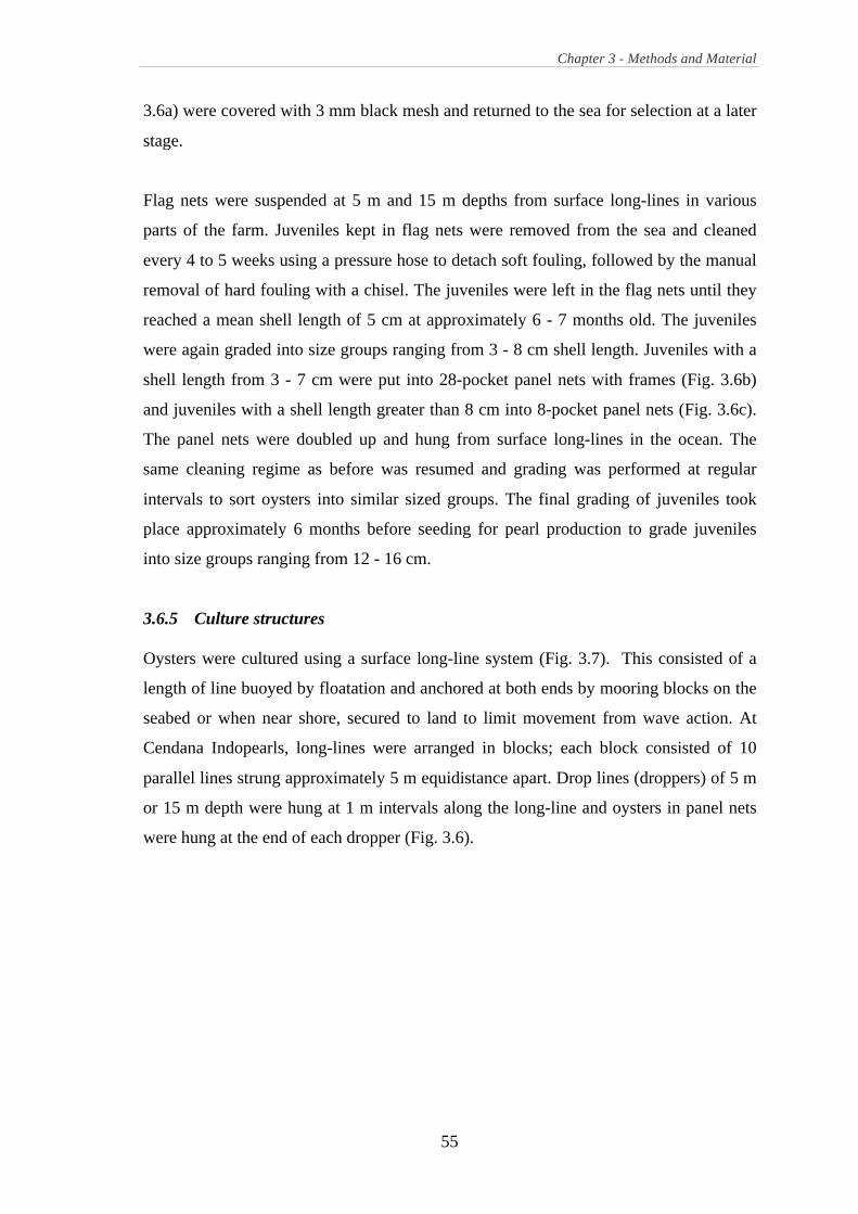
Chapter 3 - Methods and Material
55
3.6a) were covered with 3 mm black mesh and returned to the sea for selection at a later
stage.
Flag nets were suspended at 5 m and 15 m depths from surface long-lines in various
parts of the farm. Juveniles kept in flag nets were removed from the sea and cleaned
every 4 to 5 weeks using a pressure hose to detach soft fouling, followed by the manual
removal of hard fouling with a chisel. The juveniles were left in the flag nets until they
reached a mean shell length of 5 cm at approximately 6 - 7 months old. The juveniles
were again graded into size groups ranging from 3 - 8 cm shell length. Juveniles with a
shell length from 3 - 7 cm were put into 28-pocket panel nets with frames (Fig. 3.6b)
and juveniles with a shell length greater than 8 cm into 8-pocket panel nets (Fig. 3.6c).
The panel nets were doubled up and hung from surface long-lines in the ocean. The
same cleaning regime as before was resumed and grading was performed at regular
intervals to sort oysters into similar sized groups. The final grading of juveniles took
place approximately 6 months before seeding for pearl production to grade juveniles
into size groups ranging from 12 - 16 cm.
3.6.5 Culture structures
Oysters were cultured using a surface long-line system (Fig. 3.7). This consisted of a
length of line buoyed by floatation and anchored at both ends by mooring blocks on the
seabed or when near shore, secured to land to limit movement from wave action. At
Cendana Indopearls, long-lines were arranged in blocks; each block consisted of 10
parallel lines strung approximately 5 m equidistance apart. Drop lines (droppers) of 5 m
or 15 m depth were hung at 1 m intervals along the long-line and oysters in panel nets
were hung at the end of each dropper (Fig. 3.6).

Chapter 3 - Methods and Material
56
Fig. 3.6 Various nets used in the culture of P. maxima in Aljui Bay including flag nets for spat (a), 28-pocket panel nets for juveniles with 3 – 7 cm shell length (b) and 8-pocket panel nets for adult oysters with shell length > 8 cm (c).
(a) (b)
(c)

Chapter 3 - Methods and Material
57
Fig. 3.7 Diagrammatic representation of a long-line system used for the suspended culture of P. maxima at Cendana Indopearls.
Styrofoam float
Marker buoy
Mooring
block
Land anchor

Chapter 3 - Methods and Material
58
3.7 Culture of experimental oysters
Oysters used in experiments were randomly selected during grading and kept separate
from farm oysters in different nets and long-lines at experimental sites. When oysters of
a particular age or size were required to examine the effects of these parameters,
stratified random sampling was employed where the populations of oysters were first
divided into relevant groups; thereafter oysters were randomly chosen. Depending on
the experiment, the oysters were subjected to the same regular cleaning regime as other
oysters on the farm, with the difference that once an experiment commenced, oysters
were not graded according to size as per normal husbandry practice for farmed oysters.
3.8 Sampling of experimental oysters
Oysters were transferred from the ocean grow-out to the laboratory and placed upright
in oyster baskets in 1000 L raceways constantly supplied with running seawater from a
flow-through system. The oysters were kept at ambient salinity and water temperature
for no longer than 2 h before being sampled.
3.8.1 Linear growth measurements
Before linear growth sampling, oysters were cleaned of surface fouling with a knife and
dried with tissue. Shell length, shell height and shell thickness (Section 2.3.1) were
measured using a vernier calliper to the nearest 0.1 mm (Fig. 2.1 in Chapter 2). Before
measuring shell thickness, oysters were checked to ensure both valves were firmly
closed so measurement was not distorted by gaping.
3.8.2 Weight measurement
3.8.2.1 Wet weight
Before weight sampling, oysters were wiped dry with paper tissue then wet weight was
measured using a digital balance (Sartorius® LP 6200 S) to two decimal places.
3.8.2.2 Dry weight
Dry weight of oyster components was determined by sacrificing and dissecting an
oyster. The dissected oyster was separated into shell, adductor muscle, mantle, muscle
and remaining soft tissue components. The muscle, mantle and soft tissue were dab-
Chapter 3 - Methods and Material
59
dried with paper towel, placed on aluminium foil and dried in an oven at 55 °C until
constant weight. Organic content was determined by weight difference after ashing the
dried components at 400 °C for 4 h.
3.9 Statistical Analyses
All analyses were performed using Excel 2003 (Microsoft! Corp.) and SPSS Version
16.0 (SPSS© Inc.).
When an analysis of variance (ANOVA) was used, the two underlying assumptions of
ANOVA, homocedascity and normality, were tested on the data using the Levene’s and
Shapiro-Wilk’s test, respectively. In the event of a variable departing from the
assumption of homocedascity, a suitable transformation was applied. In some instances
where variance remain heteroscedastic after transformation due to outliers, analysis of
variance was performed nonetheless, as ANOVA is robust, operating well even within
considerable heterogeneity of variances as long as all n are equal or nearly equal (Zar,
1984). The test is also robust to violations of the normality assumption, provided that
the samples are sufficiently large (Francis, 2004). The significance level (") was set at
0.05 for all analysis of variance.
When two or more variables were compared, a multivariate analysis of variance
(MANOVA) was utilised using the Wilks Lambda statistic. Assumptions of MANOVA
i.e. multivariate normality and homogeneity of variance/covariance matrix was checked
using outliers testing and Box M in SPSS. Fortunately, like ANOVA, provided that the
sample sizes are equal, MANOVA is also very robust to violations of homogeneity of
variance/covariance assumptions (Francis, 2004).
Principal component analysis (PCA) is a data reduction technique that reduces observed
variables to a more meaningful and manageable number without excessive loss of
information (Francis, 2004). PCA was performed in some analysis to gain a better
understanding of the relationship among variables. Factors (components) with
eigenvalues greater than one (known as Kaiser’s criterion) were retained and rotated.
The rotation used depended on whether the factors produced were expected to be
uncorrelated (orthogonal rotation) or correlated (oblique rotation). Varimax rotation was
A

Chapter 3 - Methods and Material
60
employed where an orthogonal rotation was required while a Direct Oblimin was
selected for an oblique rotation (Francis, 2004). Each component is a composite
variable made up of a linear combination of the original variables (Appeldoorn, 1983).
In this thesis, when a new variable is created for each factor in the final solution, the
method used for calculating the factor scores was the regression method.
Discriminant analysis was performed in some analyses to predict group membership
and to identify variables that were useful in discriminating between groups (Francis,
2004). It is a multivariate technique that can be used to build rules that classify a subject
into the appropriate population. It is similar to regression analysis except that the
dependent variable is categorical rather than continuous and its objective is to be able to
predict class membership on an individual observation based on a set of predictor
variables (Steel et al., 2004).

Chapter 4 - Multivariate analysis of environmental parameters
61
CHAPTER 4
Multivariate analyses of temporal and spatial variations
in environmental parameters at three experimental sites within Aljui Bay
4.1 Introduction
Site selection is one of the most important considerations in aquaculture. Some of the
factors that need to be taken into account when choosing a site include ease of access
(e.g. proximity to land), protection from wind and wave action, security and most
importantly, an optimal environment that satisfies the growth requirements of the
cultured species. In land-based culture, the growing environment may be regulated in
tanks and raceways. In pearl oyster culture, where oysters are grown out for long
periods of time in the ocean, hydrological characteristics of the environment often exert
a significant effect on growth.
Sukhotin and Maximovich (1994) divided the effects of the environment on bivalve
growth into factors of general action and local action. The former include water
temperature and salinity, which may affect the rate of biochemical reactions within the
organism in temperate climates. Factors of local action include suspended particulate
matter (SPM), particulate organic matter (POM), chlorophyll levels, water current and
water depth that determine nutritional conditions to influence growth rate of the
organism.
Besides affecting growth and mortality, the microenvironment also has other significant
effects on bivalve culture. For example, the colour and quality of harvested pearls are of
prime importance in pearl oyster culture, and factors such as depth of culture and light
penetration, and the quality of phytoplankton have been reported to contribute to pearl
colour and quality (Sonkar, 1998) by influencing the bio-mineralisation process of
nacre (Wu et al., 2003a).
While seasonal variation in factors of general action (e.g. water temperature) is not as
distinct in the tropics as in temperate areas, there have been reports that experimental

Chapter 4 - Multivariate analysis of environmental parameters
62
production of pearls in the tropics shows differential nacre growth and pearl quality
during different periods (Victor et al., 1994).
The effects of the environment on various aspects of Pinctada maxima growth at the
research sites of Ganan, Manselo and Batu Terio are important considerations in this
study. This chapter is devoted to the multivariate analyses of temporal and spatial
effects on environmental factors of both general and local action for the duration of the
research. To avoid repeated descriptions of environmental data analyses in subsequent
chapters, this chapter also introduces the various methods employed for statistical
analyses of environmental data, provides an overall insight into the environmental
conditions in which P. maxima were cultured over a 20-month period, and examines
relationships between the various environmental parameters.
4.2 Methods and Materials
4.2.1 Environmental monitoring
Environmental parameters were measured weekly in Ganan and Batu Terio from June
2000 to February 2002. Manselo was sampled weekly from June 2000 to November
2001. Duplicate water samples (1 L) were taken at each sampling from 5 m and 15 m
depths using a suspended water sampler for measurement of salinity, pH, SPM, POM
and chlorophyll a, b, c according to the methods described in Chapter 3 (Section 3.5).
Environmental monitoring of each site corresponded to the timing of various
experiments conducted at the particular site (detailed in subsequent chapters) and
seawater was sampled close to experimental long-lines. While environmental sampling
was continuous, the whole dataset was not used in the analyses of all experiments as the
experiments were staggered and conducted within different time frames. The
corresponding environmental dataset for the relevant period will be specified in each
subsequent chapter. However, in this chapter, the complete dataset will be employed to
provide a more comprehensive picture of the variation in environmental parameters
between culture site and depth over the entire study period.

Chapter 4 - Multivariate analysis of environmental parameters
63
4.2.2 Statistical analysis
A mean value for each parameter for each site and at each depth over a particular
monthly period (Ca) was determined using Equation 3.7 in Section 3.5.7.
Means were computed using the pivot table function in Microsoft Excel 2003 and used
for graphical representation of environmental parameters from various sites, depths and
sampling months.
A univariate analysis of covariance (ANCOVA) was used to analyse each
environmental parameters to determine if they were significantly different between sites
and depths over the sampling months, with the sampling month designated the
covariate. Interaction between the covariate and factors was tested to determine
homogeneity of regression (i.e. the relationship between the covariate and the
dependent variables had the same slope in each treatment group). If the slopes were not
significantly different, the use of ANCOVA was justified (i. e. the covariate did not
have an effect on factors). Before analysis, assumptions of ANCOVA (i.e.
homocedascity and normality), were tested on the data using the Levene’s and Shapiro-
Wilk’s test, respectively, according to the methods outlined in Section 3.9.
To assess the simultaneous effects of spatial (site and depth) and temporal (month)
factors on all environmental variables, the Wilks-Lambda multivariate analysis of
covariance (MANCOVA) was performed on the complete dataset. SPM, POM, pH,
salinity, water temperature, chlorophyll a, b and c were assigned the dependent
variables, site and depth the fixed factors and month of sampling the covariate.
Pair-wise principal component analysis (PCA) was performed on the environmental
data to determine relationships between environmental variables. Components with
eigenvalues greater than one (known as Kaiser’s criterion) were retained and rotated
obliquely by Direct Oblimin method to produce components (Francis, 2004).

Chapter 4 - Multivariate analysis of environmental parameters
64
4.3 Results
Environmental data sampled from 5 m and 15 m at Ganan, Manselo and Batu Terio
from June 2000 to February 2002 are summarised in Table 4.1, Table 4.2 and Table 4.3
, respectively. Each parameter will also be discussed individually. Descriptive statistics
of each treatment are given in Appendix A.
4.3.1 Univariate analysis of environmental parameters
4.3.1.1 Water temperature
During the experimental period, seawater temperature ranged from 27.43°C to 29.87°C.
When tested with univariate ANCOVA, mean water temperature between sites, depths
and month of sampling was significantly different (site: F(2,500) = 91.349, p < 0.05;
depth: F(1,500) = 5.130, p < 0.05; month: F(1,500) = 4.610, p < 0.05). There were also
differences in water temperature between site and depth combinations as the interaction
between site and depth was significant (F(2,500) = 75.488, p < 0.05).
There appeared to be a seasonal trend in seawater temperature with average water
temperatures peaking in December 2000 and 2001 and dipping in August 2000 and
2001 at all sites and depths (Fig. 4.1). Mean water temperatures at Ganan were
consistently lower than at Manselo and Batu Terio where water temperature decreased
with depth. However, at Ganan, the water temperature was higher at 15 m than at 5 m.
Overall, the highest water temperatures were consistently recorded at Manselo at a
depth of 5 m while the lowest water temperatures were recorded at Ganan at a depth of
5 m.

Chapter 4 - Multivariate analysis of environmental parameters
65
Table 4.1 Means of various environmental parameters at Ganan at 5 m and 15 m depths. Missing data indicated by NA.
Month
Water
temperature ( °C)
Salinity
(‰)
pH
SPM
(mg L-1)
POM
(mg L-1)
Chlorophyll a
(!g L-1)
Chlorophyll b
(!g L-1)
Chlorophyll c
(!g L-1)
5 m 1 5 m 5 m 15 m 5 m 15 m 5 m 15 m 5 m 15 m 5 m 15 m 5 m 15 m 5 m 15 m
Jun 00 28.20 28.86 34.0 33.8 7.6 7.8 0.040 0.053 0.023 0.020 NA 0.616 NA 0.637 NA 1.867
Jul 00 27.96 28.75 35.2 34.8 7.9 7.9 0.042 0.034 0.020 0.010 0.58 0.514 0.726 0.569 2.047 1.528
Aug 00 27.89 28.74 35.0 35.0 8.1 8.1 0.045 0.043 0.010 0.018 0.35 0.249 0.471 0.299 1.310 0.900
Sep 00 27.92 28.74 34.8 35.0 7.8 7.8 0.033 0.038 0.015 0.018 0.30 0.267 0.390 0.381 1.052 1.048
Oct 00 28.13 28.85 34.8 34.8 7.8 7.8 0.047 0.043 0.020 0.023 0.63 0.419 0.691 0.413 1.925 1.301
Nov 00 28.89 29.16 34.5 34.3 8.0 8.0 0.078 0.083 0.058 0.060 0.69 0.454 1.019 0.296 2.637 1.020
Dec 00 29.21 29.08 35.0 34.8 7.9 7.9 0.075 0.068 0.050 0.050 0.42 0.340 0.534 0.435 1.555 1.271
Jan 01 28.71 28.72 35.0 35.0 7.7 7.7 0.070 0.068 0.048 0.048 0.60 0.413 0.717 0.499 2.102 1.386
Feb 01 28.50 28.71 35.0 35.0 7.9 7.9 0.050 0.055 0.028 0.030 0.25 0.520 0.335 0.670 0.987 1.878
Mar 01 28.36 28.74 35.0 35.0 7.8 7.8 0.053 0.050 0.025 0.033 0.45 0.439 0.717 0.681 2.040 2.001
Apr 01 28.37 28.63 36.0 35.0 NA NA 0.040 0.030 0.020 0.010 0.54 0.544 0.706 0.816 1.819 2.227
May 01 28.42 28.99 35.8 35.8 7.0 7.2 0.053 0.050 0.028 0.025 0.60 0.382 0.919 0.503 2.614 1.481
Jun 01 28.30 28.89 33.5 34.3 6.7 7.0 0.043 0.038 0.020 0.018 0.75 0.619 1.178 1.028 3.302 2.876
Jul 01 27.87 28.52 35.0 35.3 6.7 6.9 0.036 0.036 0.014 0.028 0.58 0.700 0.810 1.106 2.269 3.145
Aug 01 27.60 28.22 34.4 34.8 7.4 7.6 0.034 0.036 0.014 0.006 0.45 0.489 0.632 0.769 1.825 2.043
Sep 01 27.72 28.34 34.0 34.0 7.5 7.7 0.032 0.035 0.012 0.005 0.33 0.167 0.456 0.170 1.297 0.654
Oct 01 28.10 28.72 35.0 35.2 7.7 7.6 0.034 0.034 0.010 0.010 0.47 0.421 0.669 0.587 1.905 1.653
Nov 01 28.18 28.82 35.0 35.0 7.6 7.7 0.035 0.030 0.008 0.010 0.40 0.300 0.557 0.291 1.539 0.905
Dec 01 29.12 29.02 35.0 35.0 7.7 7.8 0.034 0.030 0.010 0.004 0.63 0.517 0.915 0.707 2.661 2.052
Jan 02 28.70 28.71 34.5 35.0 8.0 8.0 0.023 0.028 0.007 0.005 0.36 0.511 0.394 0.708 1.292 2.111
Feb 02 28.50 28.71 35.0 35.0 8.0 8.0 0.030 0.035 0.005 0.010 0.47 0.697 0.714 1.102 1.985 2.943

Chapter 4 - Multivariate analysis of environmental parameters
66
Table 4.2 Means of various environmental parameters at Manselo at 5 m and 15 m depths. Missing data indicated by NA.
Month
Water
Temperature (°C)
Salinity
(‰)
pH
SPM
(mg L-1)
POM
(mg L-1)
Chlorophyll a
(!g L-1)
Chlorophyll b
(!g L-1)
Chlorophyll c
(!g L-1)
5 m 1 5 m 5 m 15 m 5 m 15 m 5 m 15 m 5 m 15 m 5 m 15 m 5 m 15 m 5 m 15 m
Jun 00 29.25 28.81 33.0 33.0 7.7 7.7 0.033 0.033 0.020 0.015 0.626 0.715 0.719 0.903 2.100 2.502
Jul 00 28.99 28.79 34.0 34.0 8.0 8.0 0.036 0.038 0.010 0.014 0.734 0.449 1.040 0.564 2.865 1.607
Aug 00 29.07 28.75 35.0 34.8 8.1 8.1 0.030 0.030 0.010 0.013 0.303 0.399 0.403 0.576 1.149 1.607
Sep 00 29.19 28.76 34.8 35.0 7.8 7.8 0.038 0.040 0.015 0.018 0.630 0.669 0.873 0.910 2.415 2.449
Oct 00 29.24 29.10 34.3 34.5 7.8 7.8 0.045 0.050 0.015 0.023 0.489 0.470 0.460 0.323 1.339 0.976
Nov 00 29.59 29.32 33.8 34.3 8.0 8.0 0.090 0.088 0.065 0.063 0.470 0.510 0.323 0.431 0.976 1.019
Dec 00 29.58 29.25 34.8 35.0 8.0 7.9 0.068 0.070 0.045 0.050 0.593 0.326 0.733 0.325 2.123 0.961
Jan 01 29.11 28.88 35.0 35.0 7.8 7.8 0.066 0.064 0.044 0.046 0.255 0.565 0.343 0.678 1.015 1.897
Feb 01 29.13 28.72 35.0 35.0 7.9 7.9 0.050 0.043 0.025 0.015 0.434 0.437 0.534 0.644 1.458 1.865
Mar 01 29.26 28.94 35.0 35.0 7.8 7.8 0.053 0.048 0.033 0.023 0.459 0.639 0.717 0.952 1.943 2.549
Apr 01 29.34 28.88 35.0 35.0 NA NA 0.040 0.050 0.020 0.030 0.837 0.547 1.444 0.927 4.009 2.634
May 01 29.40 28.88 34.3 35.0 7.4 7.4 0.055 0.053 0.038 0.028 0.610 0.954 0.974 1.511 2.745 4.202
Jun 01 29.31 28.87 33.0 33.0 7.4 7.4 0.045 0.043 0.028 0.018 0.953 0.883 1.483 1.409 4.100 3.960
Jul 01 28.94 28.50 35.5 35.3 7.2 7.3 0.042 0.040 0.018 0.014 0.311 0.211 0.380 0.305 1.045 0.867
Aug 01 28.61 28.18 34.2 34.0 7.6 7.6 0.036 0.032 0.014 0.014 0.824 0.870 1.251 1.244 3.369 3.422
Sep 01 28.81 28.34 33.5 33.3 7.6 7.5 0.033 0.033 0.008 0.008 0.399 0.255 0.557 0.326 1.539 0.953
Oct 01 29.30 28.78 35.0 35.0 7.9 7.9 0.034 0.028 0.008 0.006 0.676 0.747 0.908 1.055 2.586 2.908
Nov 01 29.34 28.70 34.5 34.5 7.8 7.8 0.030 0.033 0.005 0.010 0.787 0.600 1.005 0.891 2.743 2.512

Chapter 4 - Multivariate analysis of environmental parameters
67
Table 4.3 Means of various environmental parameters at Batu Terio at 5 m and 15 m depths. Missing data indicated by NA.
Month
Water
Temperature (°C)
Salinity
(‰)
pH
SPM
(mg L-1)
POM
(mg L-1)
Chlorophyll a
(!g L-1)
Chlorophyll b
(!g L-1)
Chlorophyll c
(!g L-1)
5 m 1 5 m 5 m 15 m 5 m 15 m 5 m 15 m 5 m 15 m 5 m 15 m 5 m 15 m 5 m 15 m
Jun 00 29.06 28.91 33.3 33.5 7.8 7.7 0.040 0.040 0.020 0.023 0.618 0.716 0.692 0.930 2.071 2.603
Jul 00 28.88 28.67 35.0 35.0 7.9 8.0 0.038 0.040 0.010 0.016 0.770 0.658 0.950 0.800 2.685 2.114
Aug 00 28.89 28.70 35.3 35.3 8.1 8.1 0.043 0.053 0.010 0.025 0.298 0.309 0.422 0.458 1.265 1.304
Sep 00 28.99 28.85 35.0 35.0 7.8 7.8 0.045 0.035 0.020 0.010 0.327 0.543 0.442 0.802 1.246 2.176
Oct 00 29.08 28.86 34.3 34.8 7.8 7.8 0.047 0.050 0.023 0.020 0.508 0.634 0.597 0.746 1.703 2.129
Nov 00 29.47 29.30 34.3 34.8 8.0 8.0 0.085 0.080 0.065 0.055 0.725 0.486 0.677 0.377 2.031 1.034
Dec 00 29.37 29.22 35.0 35.0 7.9 7.9 0.073 0.063 0.050 0.045 0.518 0.324 0.633 0.251 1.742 0.689
Jan 01 28.94 28.80 35.2 35.2 7.8 7.8 0.068 0.070 0.048 0.052 0.516 0.298 0.685 0.337 1.971 0.999
Feb 01 29.22 28.76 35.0 35.0 7.9 7.9 0.055 0.055 0.038 0.035 0.326 0.340 0.325 0.435 0.961 1.271
Mar 01 29.12 28.93 35.0 35.0 7.8 7.8 0.055 0.055 0.030 0.038 0.267 0.436 0.408 0.607 1.162 1.730
Apr 01 29.17 28.90 35.0 35.0 NA NA 0.040 0.040 0.020 0.020 0.798 0.511 1.115 0.708 3.078 2.111
May 01 29.28 28.93 35.8 34.8 7.2 7.3 0.055 0.050 0.033 0.028 0.727 0.600 1.040 0.891 2.938 2.512
Jun 01 29.26 28.90 34.8 34.0 7.1 7.3 0.043 0.035 0.025 0.023 0.891 0.874 1.436 1.354 3.989 3.829
Jul 01 28.90 28.54 34.5 34.3 7.1 7.1 0.042 0.040 0.022 0.016 0.742 0.481 1.077 0.735 3.048 2.091
Aug 01 28.53 28.16 34.2 34.2 7.6 7.6 0.042 0.034 0.012 0.010 0.518 0.727 0.707 1.040 2.038 2.938
Sep 01 28.77 28.41 34.3 33.8 7.7 7.4 0.030 0.028 0.008 0.008 0.326 0.373 0.428 0.448 1.195 1.350
Oct 01 28.84 28.81 35.2 35.2 7.8 7.9 0.028 0.030 0.004 0.006 0.452 0.538 0.560 0.816 1.673 2.285
Nov 01 28.95 28.85 34.8 34.8 7.8 7.8 0.033 0.030 0.010 0.005 0.526 0.369 0.707 0.310 1.965 0.841
Dec 01 29.51 29.17 35.0 35.0 7.7 7.7 0.030 0.032 0.006 0.004 0.532 0.568 0.817 0.767 2.343 2.223
Jan 02 29.07 28.88 34.8 34.8 8.0 8.0 0.033 0.030 0.008 0.003 1.299 1.244 2.048 2.028 5.659 5.577
Feb 02 29.13 28.72 35.0 35.0 8.0 8.0 0.028 0.028 0.008 0.005 0.399 0.546 0.557 0.871 1.539 2.430

Chapter 4 - Multivariate analysis of environmental parameters
68
4.3.1.2 Salinity
Salinity ranged from 30‰ to 38‰ over the 20 months of sampling. While salinity
appeared to fluctuate between different months of sampling when plotted (Fig. 4.2),
statistically salinity was not significantly different between depths (F(1,438) = 0.031, p >
0.05) and over time (F(1, 438) = 4.610, p > 0.05). ANCOVA indicated that site had an
effect on salinity (F(2,483) = 7.522, p < 0.05). Differences in mean salinities were
observed between the three sites from April 2001 to August 2001. Salinity peaks were
observed at 5 m in Ganan, Manselo and Batu Terio in April 2001, July 2001 and May
2001 respectively. The lowest salinities were recorded at Ganan and Manselo at 5 m on
June 2001, while the lowest salinity at Batu Terio occurred in June 2000 at a depth of 5
m (Fig. 4.2). Post-hoc test showed that the salinity in Batu Terio was different from that
of Ganan and Manselo.
4.3.1.3 pH
The pH of seawater at the three sites over the 20-month sampling period ranged from
6.4 to 8.3. There was a significant seasonal variation in pH (F(1,447) = 38.150, p < 0.05)
while site and depth did not affect pH (site: F(2,447) = 2.459, p > 0.05; depth: F(1,447) =
0.934, p > 0.05). The lowest pH levels were recorded from May to September 2001 at
all three sites (Fig. 4.3). pH of seawater at Manselo and Batu Terio were almost
identical at 5 m and 15 m. However, pH levels in Ganan differed slightly from May
2001 to July 2001 before becoming stable for the rest of the sampling period.

Chapter 4 - Multivariate analysis of environmental parameters
69
Fig. 4.1 Spatial and temporal variation in water temperature at depths of 5 m and 15
m in Ganan, Manselo and Batu Terio over the sampling period (June 2000 – February 2002 for Ganan and Batu Terio, June 2000 – October 2001 for Manselo). Vertical bars indicate Standard Error.
Ganan
27.0
27.5
28.0
28.5
29.0
29.5
30.0
Batu Terio
27.0
27.5
28.0
28.5
29.0
29.5
30.0
Jun00
Aug00
Oct00
Dec00
Feb01
Apr01
Jun01
Aug01
Oct01
Dec01
Feb02
Month
Manselo
27.0
27.5
28.0
28.5
29.0
29.5
30.0
5m15m
Wat
er te
mpe
ratu
re (°
C)
Month

Chapter 4 - Multivariate analysis of environmental parameters
70
Fig. 4.2 Spatial and temporal variation in salinity at depths of 5 m and 15 m in Ganan, Manselo and Batu Terio over the sampling period (June 2000 – February 2002 for Ganan and Batu Terio, June 2000 – October 2001 for Manselo). Vertical bars indicate Standard Error.
Salin
ity (‰
)
Ganan
32.5
33.5
34.5
35.5
36.5
Batu Terio
32.5
33.5
34.5
35.5
36.5
Jun00
Aug00
Oct00
Dec00
Feb01
Apr01
June01
Aug01
Oct01
Dec01
Feb02
Month
Manselo
32.5
33.5
34.5
35.5
36.5
5 m15 m
Month
Salin
ity (‰
)

Chapter 4 - Multivariate analysis of environmental parameters
71
Fig. 4.3 Spatial and temporal variation in pH at depths of 5 m and 15 m in Ganan,
Manselo and Batu Terio over the sampling period (June 2000 – February 2002 for Ganan and Batu Terio, June 2000 – October 2001 for Manselo). Vertical bars indicate Standard Error.
pH
Ganan
6.5
7.0
7.5
8.0
8.5
Batu Terio
6.5
7.0
7.5
8.0
8.5
Jun00
Aug00
Oct00
Dec00
Feb01
May01
July01
Sep01
Nov01
Jan02
Month
Manselo
6.5
7.0
7.5
8.0
8.5
5 m 15 m
Month

Chapter 4 - Multivariate analysis of environmental parameters
72
4.3.1.4 SPM
SPM levels ranged from 0 - 0.15 mg L-1 during the sampling period. Statistical analysis
indicated that the levels of SPM were significantly affected by the months of sampling
(F(1, 485) = 43.904, p < 0.05) but were not significantly different between sites and depths
(site: F(2,485) = 0.78, p > 0.05; depth: F(1,485) = 0.23, p > 0.05). At all three sites, SPM
increased gradually from August 2000 and peaked in November 2000. Another smaller
peak was observed in June 2001, but overall, SPM levels remained relatively constant
throughout 2001 (Fig. 4.4).
4.3.1.5 POM
POM ranged from 0 – 0.12 mg L-1 during the experiment. As with SPM, which is the
sum of POM and particulate inorganic matter (PIM), POM levels varied significantly
over time (F(1,485) = 48.420, p < 0.05) but were not significantly different between sites
(F(2,485) = 4.258, p > 0.05) and depths (F(1,485) = 0.333, p > 0.05). As might be expected,
POM levels followed an identical distribution as SPM over time at all sites and depths,
with a large peak observed in November 2001 and a smaller peak observed in June 2001
(Fig. 4.5).
4.3.1.6 Chlorophyll a
Chlorophyll a levels ranged from 0.0 – 1.96 !g L-1. Chlorophyll a levels were
significantly different between sites (F(2,448) = 4.223, p < 0.05) but were not different
between depths (F(1,448) = 0.346, p > 0.05). While sampling month did not appear to
have an effect on chlorophyll a levels when tested with an ANCOVA (F(1,448) = 3.580, p
> 0.05), the probability (p = 0.059) was very close to " (0.05) indicating that sampling
month very likely does exert an influence on chlorophyll a levels. This was supported
by graphical data (Fig. 4.6), which showed chlorophyll a levels fluctuate over the
sampling period. Chlorophyll a levels peaked between April and August 2001 at all the
sites while the highest level of chlorophyll a was observed in Batu Terio from
December 2001 to January 2002, with mean levels reaching 1.2 !g L-1.

Chapter 4 - Multivariate analysis of environmental parameters
73
Fig. 4.4 Spatial and temporal variation in SPM at depths of 5 m and 15 m in Ganan, Manselo and Batu Terio over the sampling period (June 2000 – February 2002 for Ganan and Batu Terio, June 2000 – October 2001 for Manselo). Vertical bars indicate Standard Error.
Ganan
0.00
0.02
0.04
0.06
0.08
0.10
Batu Terio
0.00
0.02
0.04
0.06
0.08
0.10
Jun00
Aug00
Oct00
Dec00
Feb01
Apr01
June01
Aug01
Oct01
Dec01
Feb02
Month
Manselo
0.00
0.02
0.04
0.06
0.08
0.10
5 m15 m
SPM
(g L
-1)
Month
SPM
(mg
L-1)

Chapter 4 - Multivariate analysis of environmental parameters
74
Fig. 4.5 Spatial and temporal variation in POM at depths of 5 m and 15 m in Ganan,
Manselo and Batu Terio over the sampling period (June 2000 – February 2002 for Ganan and Batu Terio, June 2000 – October 2001 for Manselo). Vertical bars indicate Standard Error.
Ganan
0.00
0.02
0.04
0.06
Batu Terio
0.00
0.02
0.04
0.06
Jun00
Aug00
Oct00
Dec00
Feb01
Apr01
June01
Aug01
Oct01
Dec01
Feb02
Month
Manselo
0.00
0.02
0.04
0.06
5 m15 m
POM
(g L
-1)
Month
POM
(mg
L-1)

Chapter 4 - Multivariate analysis of environmental parameters
75
Fig. 4.6 Spatial and temporal variation in chlorophyll a at depths of 5 m and 15 m in Ganan, Manselo and Batu Terio over the sampling period (June 2000 – February 2002 for Ganan and Batu Terio, June 2000 – October 2001 for Manselo). Vertical bars indicate Standard Error.
Ganan
0.0
0.2
0.4
0.6
0.8
1.0
1.2
1.4
Batu Terio
0.0
0.2
0.4
0.6
0.8
1.0
1.2
1.4
Jun00
Aug00
Oct00
Dec00
Feb01
Apr01
Jun01
Aug01
Oct01
Dec01
Feb02
Month
Manselo
0.0
0.2
0.4
0.6
0.8
1.0
1.2
1.4
5m15m
Chl
orop
hyll
a (g
L-1
)
5 m
15 m
Month
Chl
orop
hyll
a (!
g L-1
)

Chapter 4 - Multivariate analysis of environmental parameters
76
4.3.1.7 Chlorophyll b
Chlorophyll b levels ranged from 0.0 – 3.18 !g L-1 during the sampling period.
Statistical analysis indicated that chlorophyll b levels were significantly different
between sampling months (F(1,448) = 15.812, p < 0.05) and sites (F(2,448) = 3.322, p <
0.05) but were not affected by depth (F(1,448) = 0.399, p > 0.05). Chlorophyll b levels
were higher in Batu Terio and Manselo than at Ganan, and fluctuated with no discerning
pattern throughout the sampling period at all three sites (Fig. 4.7). Between April 2001
and August 2001, levels of chlorophyll b showed several small peaks at the three sites.
As with chlorophyll a levels, the highest chlorophyll b was found at Batu Terio in
December 2001 – January 2002, with mean levels > 2 !g L-1 recorded.
4.3.1.8 Chlorophyll c
Chlorophyll c was found in greater concentration than chlorophyll a and chlorophyll b
at all three sites, with concentration ranging from 0.0 – 8.5 !g L-1. Chlorophyll c levels
were significantly different in seawater sampled between different months (F(1,448) =
16.469, p < 0.05) and from different sites (F(2,448) = 3.036, p < 0.05), but was the same
for the two depths (F(1,448) = 0.472, p > 0.05). As with chlorophyll a and chlorophyll b,
chlorophyll c levels were highest in the period between December 2001 to January 2002
at Batu Terio reaching concentrations exceeding 5 !g L-1, while smaller peaks between
3 – 4 !g L-1 were observed between April and August 2001 at all sites (Fig. 4.8).
4.3.1.9 Rainfall
There was significant temporal variation in rainfall during the sampling months (F(17,428)
= 7.326, p < 0.05). There did not appear to be a distinct annual wet or dry season during
the 20 months of sampling, with the highest rainfall recorded in June 2000 and the
lowest rainfall recorded in August 2001 (Fig. 4.9).

Chapter 4 - Multivariate analysis of environmental parameters
77
Ganan
0.0
0.4
0.8
1.2
1.6
2.0
Batu Terio
0.0
0.4
0.8
1.2
1.6
2.0
Jun 00
Aug 00
Oct 00
Dec 00
Feb 01
Apr 01
Jun 01
Aug 01
Oct 01
Dec 01
Feb 02
Month
Manselo
0.0
0.4
0.8
1.2
1.6
2.0
5 m 15 m
Chl
orop
hyll
b (!
g L-1
)
Fig. 4.7 Spatial and temporal variation in chlorophyll b at depths of 5 m and 15 m in Ganan, Manselo and Batu Terio over the sampling period (June 2000 – February 2002 for Ganan and Batu Terio, June 2000 – October 2001 for Manselo). Vertical bars indicate Standard Error.

Chapter 4 - Multivariate analysis of environmental parameters
78
Fig. 4.8 Spatial and temporal variation in chlorophyll c at depths of 5 m and 15 m in
Ganan, Manselo and Batu Terio over the sampling period (June 2000 – February 2002 for Ganan and Batu Terio, June 2000 – October 2001 for Manselo). Vertical bars indicate Standard Error.
Batu Terio
0.0
1.0
2.0
3.0
4.0
5.0
6.0
Jun00
Aug00
Oct00
Dec00
Feb01
Apr01
Jun01
Aug01
Oct01
Dec01
Feb02
Month
Ganan
0.0
1.0
2.0
3.0
4.0
5.0
6.0
Manselo
0.0
1.0
2.0
3.0
4.0
5.0
6.0
5m15m
Chl
orop
hyll
c (g
L-1
)
5 m
15 m
Month
Chl
orop
hyll
c (!
g L-1
)

Chapter 4 - Multivariate analysis of environmental parameters
79
Fig. 4.9 Temporal variation in rainfall at all sites over sampling period (June 2000 – February 2002). Vertical bars indicate Standard Error.
4.3.2 Multivariate analysis of environmental parameters
Results of the MANCOVA showed that overall, site (F(16,762) = 3.614, p < 0.05) and
month of sampling (F(8,380) = 0.796, p < 0.05) had an effect on environmental parameters
while depth (F(8,380) = 0.552, p > 0.05) did not. However, there was significant
interaction between site and depth (F(16,762) = 0.909, p < 0.05) indicating that there were
differences in environmental parameters between depths at various sites.
Test of between subjects effect indicated that site had a significant effect on water
temperature (F(2,387) = 21.743, p < 0.05) and salinity (F(2,387) = 3.231, p < 0.05) while
sampling month affected water temperature (F(1,387) = 6.445, p < 0.05), salinity (F(1,387) =
5.558 , p < 0.05), pH (F(1,387) = 27.384 , p < 0.05), SPM (F(1,387) = 30.877, p < 0.05),
POM (F(1,387) = 35.557, p < 0.05), chlorophyll b (F(1,387) = 12.127, p < 0.05) and
chlorophyll c (F(1,387) = 12.561, p < 0.05). Depth did not exert any significant effect on
any of the environmental parameters.
0
100
200
300
400
500
600
Jun00
Aug00
Oct00
Dec00
Feb01
Apr01
Jun01
Aug01
Oct01
Dec01
Feb02
Month
Rai
nfal
l (m
m)
Month
Rai
nfal
l (m
m)

Chapter 4 - Multivariate analysis of environmental parameters
80
4.3.3 Interrelationship between environmental parameters
The results of PCA are shown in Fig. 4.10 and Table 4.4. Four principal components
were extracted and accounted for a total of 82.92% of the original variance. The
loadings for each component given in Table 4.4 represent the partial correlation
between the variable and the rotated component. Chlorophyll a, b, c were extracted with
strong loadings with component 1. SPM and POM strongly loaded with component 2.
Components 1 and 2 variables relate to the phytoplankton and other organic food
sources in the seawater sampled. Component 3 had moderately strong loadings on pH
and rainfall and a moderate loading on water temperature, while component 4 had very
strong loading on salinity. Component 3 and 4 can be inferred as the physical
components of the seawater sampled. There were significant correlations between the
environmental parameters (Table 4.5), with the exception of salinity, which was not
significantly correlated to any of the other parameters.
Fig. 4.10 Component plot of environmental parameters in rotated space.
1.01.0
-.5
0.0
.5.5
.5
1.0
0.00.0-.5-.5
Component 1
Component 3
Component 2
Rainfall
pH
Salinity
Water temperature
Chlorophyll b Chlorophyll c
POM SPM
Chlorophyll a
Component 4

Chapter 4 - Multivariate analysis of environmental parameters
81
Table 4.4 Rotated component matrix of PCA on environmental data. Rotation method: Direct Oblimin with Kaiser normalisation. Absolute partial correlation values less than 0.1 are suppressed.
Environmental
parameter
Principal components
Communality
1
2
3
4
Chlorophyll c 0.993 0.988
Chlorophyll b 0.992 0.987
Chlorophyll a 0.978 0.959
POM 0.957 0.919
SPM 0.956 0.919
pH 0.150 0.748 0.158 0.628
Rainfall 0.214 0.720 0.615
Water temperature 0.439 0.554 0.475
Salinity 0.984 0.973
Initial eigenvalues 3.063 2.027 1.358 1.014
% Variance 34.03 22.52 15.09 11.27
% Cumulative variance 34.03 56.56 71.65 82.92

Chapter 4 - Multivariate analysis of environmental parameters
82
Table 4.5 Correlation matrix from principal component analysis of environmental parameters. Asterisk (*) indicates significant correlation. Partial correlation < 0.1 have been suppressed.
Water Temperature Salinity pH SPM POM Chlorophyll a Chlorophyll b Chlorophyll c Rainfall
Correlation Water temperature 1.000 0.229 0.256 0.264 0.066 0.107
Salinity 1.000
pH 0.229 1.000 0.128 -0.124 -0.199 -0.202 0.248
SPM 0.256 0.128 1.000 0.922 -0.155 -0.153 -0.140
POM 0.264 0.922 1.000 -0.135
Chlorophyll a -0.124 1.000 0.957 0.956
Chlorophyll b -0.199 -0.155 0.957 1.000 0.996
Chlorophyll c -0.202 -0.153 0.956 0.996 1.000
Rainfall 0.107 0.248 -0.140 -0.135 1.000
Significance Water temperature 0.428 0.000* 0.000* 0.000* 0.082 0.382 0.316 0.013*
(1-tailed) Salinity 0.428 0.127 0.305 0.379 0.380 0.336 0.346 0.158
pH 0.000* 0.127 0.003* 0.036* 0.006* 0.000* 0.000* 0.000*
SPM 0.000* 0.305 0.003* 0.000* 0.019* 0.000* 0.001* 0.002*
POM 0.000* 0.379 0.036* 0.000* 0.207 0.020* 0.019* 0.003*
Chlorophyll a 0.082 0.380 0.006* 0.019* 0.207 0.000* 0.000* 0.103
Chlorophyll b 0.382 0.336 0.000* 0.000* 0.020* 0.000* 0.000* 0.297
Chlorophyll c 0.316 0.346 0.000* 0.001* 0.019* 0.000* 0.000* 0.185
Rainfall 0.013* 0.158 0.000* 0.002* 0.003* 0.103 0.297 0.185

Chapter 4 - Multivariate analysis of environmental parameters
83
4.4 Discussion
This study presents the usefulness of multivariate statistical techniques for evaluation
and interpretation of large complex water quality data sets and apportionment of
variance factors to sites and depths in order to deduce better information about the water
quality at different sites within the pearl farm.
The choice of Ganan, Manselo and Batu Terio as experimental sites was based on a few
considerations. They are used extensively for commercial pearl oyster culture and as
such, are sites of interest. Another consideration was to determine if different
topography and positions of the three sites within Aljui Bay (Fig. 4.11) resulted in a
spatial difference in hydrological parameters.
Fig. 4.11 Diagram of the experimental sites of Ganan, Manselo and Batu Terio within
Aljui Bay, western Waigeo. Diagram is not to scale.

Chapter 4 - Multivariate analysis of environmental parameters
84
Water quality monitoring typically involves the sampling of three main categories of
hydrological descriptors: physico-chemical (water temperature, salinity, dissolved
oxygen, pH and turbidity), particulate matter (total suspended matter, organic
phosphate, nitrogen and carbon, chlorophyll pigments) and nutrients (nitrite, nitrate,
ammonium, phosphate and silicate) (Aminot et al., 2004). For the scope of this study,
only certain physico-chemical and particulate descriptors were monitored i.e. water
temperature, salinity, pH, suspended particulate matter (SPM), particulate organic
matter (POM) and chlorophyll a, b and c, as these have been reported to influence
growth of pearl oysters (Lucas, 2008b) (see Table 5.1).
Univariate analysis allowed subtle differences in an environmental variable between
different sites and depths and months of sampling to be compared without taking into
consideration possible interaction with other environmental variables.
Results showed that water temperature at the three sampling sites and two depths was
significantly different. The differences are likely accounted for by different levels of
solar warming at various depths, different topography of the sites that impacted directly
on how seawater is circulated and exchanged, as well as any upwelling of cold water at
the sites. Manselo recorded the highest mean water temperature (29.59°C) and smallest
water temperature range (1.83°C) of the three sampling sites. Its position of being
closest to land and enclosed in a small bay (Section 3.4.2) produced poor water
exchange and would account for its higher and less variable water temperature. Batu
Terio’s position in a channel (Section 3.4.3) ensured there was greater water movement
at that site leading to greater variation in temperature range (1.99°C) over the sampling
period. At both sites, water temperature at 5 m was consistently higher than water
temperature at 15 m due to the effects of solar warming higher in the water column.
This was not observed at Ganan where the average water temperature at 15 m was
found to be higher than 5 m over the sampling period. This apparent anomaly at Ganan
was associated with coastal current or cold water upwelling at the site, similar to that
along the north coast of Papua New Guinea northern where upwelling of relatively cold
water was reported (Hasegawa et al., 2008). Ganan is positioned at the entrance of Aljui
Bay and strong upwelling currents sweeping in from the Pacific Ocean from two
direction (Section 3.4.1 and Fig. 4.11) resulted in very high water exchange at the site.

Chapter 4 - Multivariate analysis of environmental parameters
85
Salinity in surface seawater was significantly different between sites. Variation in ocean
salinity is caused by a combination of factors including the relative amount of
evaporation and precipitation, proximity to freshwater run-offs, wind action and
topography of the seabed. Although sampling month did not have a significant effect on
salinity, the lowest salinity was recorded at the start of the experiment in June 2000,
which coincided with the highest rainfall recorded over the sampling period. The
proximity of experimental sites to various islands would most likely expose the sites to
freshwater run-offs and decrease overall salinity within the area during heavy rainfall.
Post-hoc tests showed that Batu Terio had different salinity than Ganan and Manselo,
which was likely caused by the variation in topography of the various sites.
The pH of seawater can be affected by several factors such as the benthic composition
through which the seawater moves and the amount of marine plant growth and organic
material in the microenvironment. In this study where the sites were located close to
shore, pH values would additionally be related to the tidal flow and the acidity of the
soils, which discharge into the sea during heavy rainfall (Sanderson and Taylor, 2003).
There was no spatial effect on pH levels observed in this study but pH levels showed
temporal variation over the sampling period. The variation in pH ranged from 6.4 to 8.3,
indicating that the seawater pH varied from acidic to alkaline. Factor analysis indicated
that pH levels in Aljui Bay were correlated to rainfall, which also differed significantly
between months. pH level fell below 7.5 when rainfall fell below 100 mm month-1 (Fig.
4.3 and Fig. 4.9). It is likely that the soil on the islands surrounding the experimental
sites is alkaline in nature, as freshwater run-off from land appeared to cause the
seawater pH to increase when precipitation was high.
SPM levels were not affected spatially (site or depth) but showed significant variation
over time. Various fluvial, oceanographic, biological and chemical factors including
tidal flow, river discharge and interaction between fresh and salt water (Sanderson and
Taylor, 2003) can affect the concentration of SPM in near-shore seawater. It has also
been reported that SPM can be influenced by biogenous components that fluctuate
seasonally and were concentrated in areas where upwelling occurs (Chester and Stoner,
1972). SPM in seawater is very heterogeneous in composition and varies in particle size
and abundance over various habitats (Lucas, 2008b), and is made up of particulate
inorganic matter (PIM) and particulate organic matter (POM). PIM is often composed

Chapter 4 - Multivariate analysis of environmental parameters
86
of resuspended benthic sediments, while POM may be derived from many sources
including phytoplankton, terrestrial material, river run-offs, resuspension of sediments
or aeolian inputs (Degens and Ittekkot, 1985) as well as non-living biogenous material
such as faeces, decomposing cells and mucus (Lucas, 2008b). In this study, distribution
of POM followed an identical distribution to SPM where there was a temporal but not
spatial effect on concentration of POM. Varying levels of SPM and POM were likely
related to both local factors, such as discharge from the land and tidal flow, as well as to
more regional climatic factors – for example, variation of seasonal solar heating over
Asia and Australia that drives the monsoon twice a year (Tomascik et al., 1997;
Webster et al., 1998).
Chlorophyll levels were found to fluctuate between sites and between months of
sampling, but not between depths. Chlorophyll concentration is an indication of the
biomass of phytoplankton in seawater and can be affected by similar factors which
influence SPM and POM concentrations, namely tidal flow, river discharge and
interaction between fresh and salt water. In addition, light is an important factor
affecting growth and multiplication of phytoplankton (Li et al., 1999). The lack of a
significant difference in the vertical distribution of phytoplankton may be due to both
depths of 5 m and 15 m lying within the euphotic zone, or to the occurrence of
upwelling causing mixing of POM in the water column.
In this study, four principal components were extracted which accounted for a total of
82.92% of the original variance. PCA showed that there were significant correlations
between the various environmental parameters. As expected, there was a very strong
correlation between SPM and POM as SPM is partly derived from POM. Similarly,
chlorophyll levels were significantly correlated to POM, as phytoplankton represent part
of the organic component measured in SPM. This is an example of how one
environmental parameter directly influences the concentration of another.
While PCA is useful for examining relationships between environmental parameters, it
does not give any indication of the way in which the environmental parameters might be
related. However, certain inferences may be made e.g. while there was a significant
correlation between POM and chlorophyll levels in this study, the partial correlation
was relatively weak (r < 0.01), indicating that phytoplankton might not make a big

Chapter 4 - Multivariate analysis of environmental parameters
87
contribution towards POM in this study, and that the organic component of SPM might
be derived from other sources, e.g. terrestrial run-offs. In a study by Fernandes et al.,
(2008), a significant positive correlation of chlorophyll a with concentrations of
particulate organic carbon (POC) was taken as an indication that phytoplankton
abundance played an important role in controlling the concentration of POC.
In summary, this chapter describes the physico-chemical characteristics and particular
matter at the two depths within the three experimental sites used in this study. These
data will provide the basis for comparison of growth rates of P. maxima held at the three
sites described in later chapters.

Chapter 5 – Temporal and spatial effects on growth
88
CHAPTER 5
Temporal, spatial and age-related growth variation and mortality
in cultured P. maxima, with emphasis on environmental influence
5.1 Introduction
A prime aim of most aquaculture industries is to achieve maximum growth rate and to
shorten grow-out time thus increasing the efficiency of production. While this aim is
true for the nursery and grow-out phases of farming P. maxima, there are stages in the
culture of pearl oysters in which slow growth is preferable; for example, in the pre-
operative stage where pearl oysters are conditioned to be weak so as not to reject an
inserted nucleus (Gervis and Sims, 1992; Taylor and Strack, 2008). While land-base
culture using raceways, tanks or ponds can be utilised to manipulate and create a
controlled growing environment, this is not an economically feasible option for pearl
oysters, which are usually grown on long-lines, fence-lines, rafts or trestles in the sea
(Gervis and Sims, 1992; Southgate, 2008). The practical alternative to a controlled land-
based culture environment is to choose a grow-out site with favourable environmental
conditions. The selection of a particular culture site or culture depth allows some
control over the growth environment of cultured pearl oysters.
Growth variability in a population of molluscs living in the same locality has been
reported to be related to differences in the microenvironments (Wilbur and Owen,
1964). This has been described for the Pacific oyster C. gigas (Brown and Hartwick,
1988b; Almeida et al., 1997, Park et al., 1999), the mussel M. edulis (Incze et al., 1980)
and the American oyster C. virginica (Mallet and Haley, 1983a; Bataller et al., 1999). It
has been also reported for the pearl oysters P. fucata (Alagarswami, 1970;
Nalluchinnappan et al., 1982), P. margaritifera (Friedman and Southgate, 1999), P.
maxima (Saville-Kent, 1893; Gervis and Sims, 1992; Sims, 1993) and Pteria penguin
(Smitasiri et al., 1994). A further selection of literature on the effects of different
environmental parameters on the growth of various species of pearl oysters is presented
in Table 5.1.

Chapter 5 – Temporal and spatial effects on growth
89
Table 5.1 Environmental parameters investigated for their influence on physiology and growth of pearl oyster.
Environmental parameter
Species
Authors
Water temperature P. maxima Yukihira et al. (2000) Mills (2000) Pass et al. (1987) P. imbricata O’Connor and Lawler (2004a) O’Connor and Lawler (2004b) Tomaru et al. (2002b) P. margaritifera Pouvreau et al. (2000c) Yukihira et al. (2000) Doroudi et al. (1999a) Pteria sterna Del Rio-Portilla et al (1992) Araya-Nuñes et al. (1991) Salinity P. maxima Kvingedal et al. (2008) P. imbricata O’Connor and Lawler (2004a) Urban (2000) P. margaritifera Doroudi et al. (1999a) pH P. maxima Taylor et al., (1997b) Welladsen (2009) P. imbricata Yu et al. (1998) Yu et al., (1999) Suspended particulate matter P. maxima Yukihira et al. (1999) Taylor et al. (1998) Taylor et al. (1997b) Rose and Baker (1994) P. imbricata Hashimoto and Nakano (2003) Tomaru et al, (2002a) Urban (2000) P. margaritifera Pit and Southgate (2000) Yukihira et al. (2000) Doroudi et al. (1999b) Southgate et al. (1998) Chlorophyll P. imbricata Tomaru et al. (2002b) P. margaritifera Vacelet et al. (1996)

Chapter 5 – Temporal and spatial effects on growth
90
Growth in marine bivalves is affected by the interaction of several environmental
variables, particularly water temperature and food supply (Incze et al., 1980; Bayne and
Newell, 1983; Brown and Hartwick, 1988b). Growth studies have generally involved
univariate empirical methods that manipulate environmental conditions in the laboratory
or field experiments that monitor variations in these variables (Malouf and Breese,
1977; Bayne and Newell, 1983 and MacDonald and Thompson, 1985). These studies
indicate that water temperature, food, salinity and pH all influence growth in bivalves
(Bernard, 1983; Bamber, 1987, 1990; Al-Sayed et al., 1997). It is clear that bivalve
growth is a function of several environmental variables acting in concert.
In addition to environmental parameters, the age of a bivalve also influences growth.
Growth rate has been reported to decrease with age in the pearl oysters, Pinctada
radiata (Nayar and Al-Rumaidh, 1993), P. margaritifera (Pouvreau et al., 2000a) and
P. mazatlanica (Saucedo and Monteforte, 1995).
While univariate studies are useful in determining differences in growth caused by age
or a particular environmental factor, it has limitations as interaction between parameters
and age, apportionment of environmental factors or age towards growth, and the degree
a particular variable affects growth are unknown. The method of choice for studies,
which involve numerous variables whose effects on, or relationships with, other
variables of interest is multivariate statistical techniques.
The research in this chapter was undertaken to establish if culture site, depth and oyster
age had a significant impact on the growth of P. maxima cultured in commercial grow-
out systems in West Papua, Indonesia.
5.2 Methods and materials
The experiment was conducted at Cendana Indopearls’ farm at Aljui Bay in West
Papua, Indonesia (refer Section 3.1) from May 2000 to November 2001.
5.2.1 Sites
Ganan, Manselo and Batu Terio (refer Section 3.4) were used as sites for the
experiments. Within each site, a longline was established to culture the oysters used in
the experiments according to the methods described in Section 3.6.5.

Chapter 5 – Temporal and spatial effects on growth
91
5.2.2 Oysters used in experiments
Hatchery produced oysters were reared according to the methods set out in Section 3.6.
Oysters were randomly selected from three age classes of oysters spawned on January
1997, February 1999 and October 1999. At the start of the experiment in June 2000, the
ages of the three groups were 41 months (3.4 years), 16 months (1.3 years) and 8
months (0.6 year); they had mean initial lengths of 153.03 ± 16.69 mm, 93.94 ± 5.04
mm and 65.66 ± 9.69 mm, respectively, when the study commenced. Size is assumed to
be a factor of age in this study; therefore, oysters from the three age classes will be
referred to as ‘large’, ‘medium’ and ‘small’ in this chapter. One hundred and fifty
oysters were randomly selected from each age class and tagged by attaching labelled
Dymo® tape to the left valve of the shells using marine epoxy. In total, 450 oysters were
tagged.
5.2.3 Experimental design
Tagged oysters from each of the three age cohorts were divided into three groups
consisting of 50 oysters and each group was allocated to Ganan, Manselo or Batu Terio
for grow-out. At each site, tagged oysters from each age group were further divided into
two groups consisting of 25 oysters per group, divided equally into five sub-groups of
five oysters and placed in doubled-up 28-pocket panel nets. The remaining spaces in the
28-pocket panel nets were filled with untagged oysters from the same age group for
fouling studies (Chapter 7). Five panel nets of oysters were hung from the long-line at a
depth of 5 m below the surface, while the other five were hung 15 m below the surface
(Error! Reference source not found.). Each treatment group was made of a different
combination of variables (i.e. site, depth and age) as outlined in Error! Reference
source not found.. In total, there were 18 treatment groups comprising of 5,040 oysters
in which 450 oysters were tagged for the growth study. During the experiment, the
oysters were not subject to the normal grading and cleaning husbandry practice
undertaken at the farm and were instead cleaned during sampling.

Chapter 5 – Temporal and spatial effects on growth
92
Fig. 5.1 Diagrammatic representation of the experiment. An example of a site/depth/site treatment group is shown in the square.
At each experimental site:
Tagged oysters
Untagged oysters
Medium
Small
Large
15 m
Styrofoam float
Marker buoy
Surface longline
Mooring block
5 m
e.g. Ganan 5 m
Large

Chapter 5 – Temporal and spatial effects on growth
93
Ganan 5 m
Large
Manselo 5 m
Large
Batu Terio 5 m
Large
Ganan 5 m
Medium
Manselo 5 m
Medium
Batu Terio 5 m
Medium
Ganan 5 m
Small
Manselo 5 m
Small
Batu Terio 5 m
Small
Ganan 15 m Large
Manselo 15 m Large
Batu Terio 15 m Large
Ganan 15 m
Medium
Manselo 15 m
Medium
Batu Terio 15 m
Medium
Ganan 15 m Small
Manselo 15 m Small
Batu Terio 15 m Small
Fig. 5.2 Site, depth and size treatment groups for the experiment. There were 18
treatment groups, with each treatment consisting of 25 tagged oysters distributed equally between five double-hung 28-pocket panel nets.

Chapter 5 – Temporal and spatial effects on growth
94
5.2.4 Sampling of oysters
Sampling was performed monthly from May 2000 to November 2001, with the
exception of December 2000 when bad weather prevented sampling. Oyster nets were
removed from long-lines and placed in a 1000 L tank constantly supplied with running
seawater piped directly from the sea, and maintained in this flow- through system at
ambient salinity and water temperature until sampled.
Both tagged and untagged oysters were removed from the panel nets by cutting through
the byssal threads attaching oysters to the net with a razor. Oysters were then cleaned of
surface biofouling with high-pressure water spray and scraped with a knife.
5.2.5 Oyster growth
Tagged oysters were measured for shell length (antero-posterior measurement, refer
Section 2.6.1.2) to the nearest 0.1 mm using vernier callipers according to the method
described in Section 3.8.1. Wet weight of each tagged oyster was measured to the
nearest 0.01 g following the method described in Section 3.8.2.
5.2.6 Oyster mortality
The number of mortalities of tagged oysters was recorded during sampling. Dead
oysters were removed from the panel nets, cleaned and placed back into the net for
fouling studies (Chapter 7) and were not replaced with live oysters. Mortality was
recorded as the number of dead oysters per month as well as calculated as overall
percentage survival.
5.2.7 Condition index (CI)
Two randomly selected untagged oysters from each treatment group were sacrificed
every month during the experiment. The oysters were cleaned of surface fouling and
total dry tissue and shell weight were determined according to the methods described in
Section 3.8.2.2. CI was calculated using the formula of Walne and Mann (1975):
(Equation 5.1)
1000 x weight Dry shell
weight tissue total Dry index Condition ! !
"
# $ $ %
& =

Chapter 5 – Temporal and spatial effects on growth
95
Dry tissue weight was measured as the sum of soft tissue, mantle and muscle dry
weight.
5.2.8 Environmental monitoring
Environmental parameters were measured weekly from June 2000 to November 2001
according to the methods described in Section 3.5. As there was no growth sampling in
December 2000, the corresponding environmental data for that month were excluded
from the analysis. A mean value for each environmental parameter at each of the three
sites and two depths over a particular sampling month (Ca) was determined using
Equation 3.7 in Section 3.5.7 and used for graphical representation of environmental
data in this chapter.
5.2.9 Statistical analyses
To measure overall growth, total growth (GT) over the sampling period was calculated
as:
(GT)= Gn – G1, (Equation 5.2)
where Gn = measurement at last sampling and G1 = measurement at first sampling.
The units for GT length and GT weight are mm and g, respectively. To determine if
oyster age, culture site and culture depth significantly affected GT, GT length and GT
weight were entered into a multivariate analysis of variance (MANOVA) using the
Wilks Lambda test of significance. Means were tested using the Bonferroni post-hoc
range test to determine which means differ.
When comparing monthly growth of tagged oysters, the absolute measurement of the
oysters was unsuitable as there were obvious size differences between the various age
classes. Instead, a more standard measure, monthly instantaneous growth rate, (G30) was
used to compare growth of oysters over a particular month and was defined by Brown
(1988) as:
(Equation 5.3) 30
DlogG
GlogG t
1t
30 !
""""
#
$
%%%%
&
'()
*+,
-
=
+
e
e

Chapter 5 – Temporal and spatial effects on growth
96
Where Gt+1 = mean growth measurement (length or weight) of the current month; Gt =
mean growth measurement of the previous month and D = number of days between
observations.
Loge transformation of D served to further detrend residuals in multiple regression
analysis (Brown, 1988). The unit of measurement for G30 length is mm month-1 and for
G30 weight g month-1. The terms ‘total growth’ and GT, as well as ‘growth rate’ and G30
are used interchangeably.
To examine the effects of sampling month, oyster age, culture site and culture depth on
G30 length and G30 weight, pair-wise repeated measure ANOVA using the Wilks
Lambda multivariate test of significance was employed using month as a repeated
measure. Besides the usual assumptions for ANOVA, the assumption for sphericity was
also tested using Mauchly’s test. If the assumption was violated, the Greenhouse-
Geissner (!) adjustment test was used (Francis, 2004).
Analysis of mortality using full factorial ANOVA with 4-way interaction could not be
employed due to insufficient replication of data as only one count of mortality (number
of dead oysters per month) could be recorded at each sampling. Instead, a main effect
and 3-way factorial ANOVA model was employed. Similarly, CI was examined using
ANOVA to test for significant differences between the different sites, depths, size and
month. The site and depth combinations, which produced the best growth for each size
class of oysters, were identified by calculating the average G30 for each site/depth
combination.
To determine the relationship between growth and environmental parameters, average
G30 of length and weight were entered into a multivariate stepwise regression with
environmental parameters assigned the independent variables. The criteria set for F to
enter and F to remove were ! 0.05 and " 0.10, respectively. Regression against
environmental parameters was tested for all oysters as well as different sized oysters
grown at the various sites and depths. Potential predictor environmental variables
included in the analysis were water temperature, salinity, pH, levels of chlorophyll a, b,
c, SPM and POM. Rainfall was not included in the analyses, as only temporal data for

Chapter 5 – Temporal and spatial effects on growth
97
rainfall was available with spatial data not sampled. Variables not included in the
equations were rejected in favour of remaining variables at ! = 0.05.
5.3 Results
Growth is discussed in terms of the total growth GT as well as monthly instantaneous
growth rate, G30.
5.3.1 Total Growth (GT)
Mean shell length and mean wet weight increased in oysters of all sizes and grown at
every site and depth over the sampling period (Table 5.2). Final mean length at the end
of the experiment in November 2001 ranged from 96.01 ± 18.18 mm (mean ± SD) for
medium oysters grown at Ganan at a depth of 15 m to 205.93 ± 32.43 mm for large
oysters grown at Ganan at a depth of 5 m. Mean length () and weight () of oysters from
different treatments were graphed over time on a standard Y axis scale to allow for
visual comparison of growth between different sized oysters.
Length growth in small oysters showed a steeper growth trajectory than that of medium
and large oysters regardless of culture site or depth. The magnitude of growth, seen by
the height difference between the initial and final length measurement, was also largest
in small oysters, indicating shell growth was greater in small oysters than in medium
and large oysters over the experimental period. Similarly, medium oysters consistently
had a steeper slope curve than large oysters. While site and depth differences were also
observed in shell growth curves, they were not as obvious as that seen for oysters of
different sizes (). Total growth was not perceivably greater at depths of 5 m or 15 m or
at any particular site when observed in the graph. When mean GT was calculated,
oysters at Manselo grew more at 5 m than at 15 m for all size groups (Table 5.3)
This was also observed in GT of small oysters at Ganan and Batu Terio. However, with
large and medium oysters, some exceptions were observed. For example, average GT
length of large oysters grown at Batu Terio at a depth of 15 m was 105.40 ± 12.70 mm
compared to 100.00 ± 15.48 mm for oysters cultured at 5 m.

Chapter 5 – Temporal and spatial effects on growth
98
Table 5.2 Mean (± SD) initial, final and GT length and weight of three size classes of P. maxima grown at Ganan, Manselo and Batu Terio.
Site
Size
Large
Medium Small
Length (mm)
Weight (g)
Length (mm)
Weight (g)
Length (mm)
Weight
(g)
Ganan Initial 149.86 (19.48)
439.49 (129.99)
94.39 (6.02)
114.22 (14.50)
53.03 (9.85)
20.79 (7.54)
Final 170.23 (16.51)
645.96 (172.48)
147.72 (14.77)
376.00 (84.68)
149.89 (9.28)
313.42 (43.10)
GT 20.36 (12.29)
206.47 (99.46)
53.32 (14.47)
261.79 (69.41)
96.86 (15.50)
292.63 (71.92)
Manselo Initial 156.08 (16.48)
571.99 (159.37)
93.74 (5.18)
115.77 (13.55)
57.16 (7.35)
25.45 (8.18)
Final 166.53 (13.97)
742.81 (126.59)
155.35 (14.54)
473.05 (83.04)
156.56 (13.05)
416.87 (68.77)
GT 10.45 (8.06)
170.82 (101.14)
61.61 (14.13)
357.28 (80.68)
99.40 (15.33)
391.43 (65.88)
Batu Terio Initial 153.16 (13.28)
495.87 (81.68)
93.68 (3.72)
116.59 (12.54)
51.61 (7.14)
19.49 (7.54)
Final 169.97 (16.63)
677.79 (178.45)
151.03 (11.09)
452.28 (57.76)
152.57 (14.95)
337.17 (91.14)
GT 16.81 (11.67)
181.92 (140.92)
57.35 (12.89)
335.69 (60.72)
100.96 (14.65)
317.68 (90.94)

Chapter 5 – Temporal and spatial effects on growth
99
MANOVA (Appendix 5.1) indicated that oyster size, culture site and culture depth had
an effect on both GT length and weight (size: F(4,576) = 265.975, p < 0.05; site: F(4,576) =
6.292, p < 0.05; depth: (F(2,288) = 5.922, p < 0.05). Between subject results showed that
GT length was significantly affected by culture depth (F(1,289) = 11.153, p < 0.05) and
oyster size (F(2,289) = 839.420, p < 0.05) but not culture site. However, there was
significant interaction between site and size (F(4,289) = 4.551, p < 0.05). GT weight was
significantly affected by oyster size (F(2,289) = 60.796, p < 0.05) and culture site (F(2,289)
= 11.005 , p < 0.05) but there was no difference in GT weight between culture depth.
Interaction between site and size was significant (F(4,289) = 7.542, p < 0.05).
Bonferroni post-hoc tests (Appendix 5.1) on sites indicated that GT weight was different
between oysters from Ganan and Manselo. Similar multiple comparisons on size
showed that GT length differed between large, medium and small oysters while GT
weight was only different between small and large oysters. Graphical representations of
GT length (Error! Reference source not found.) and GT weight (Fig. 5.6) show the
differences between sizes, sites and depths, while statistical results are summarised in
Table 5.4.

Chapter 5 – Temporal and spatial effects on growth
100
Large
Leng
th (m
m)
Medium
Small
Ganan Manselo Batu Terio
Fig. 5.3 Mean (± SE) monthly length of three size (age) classes of P. maxima grown at Ganan, Manselo and Batu Terio at 5 m ( ) and 15 m ( ) from May 2000 to November 2001.
40
60
80
100
120
140
160
180
40
60
80
100
120
140
160
180
40
60
80
100
120
140
160
180
40
60
80
100
120
140
160
180
May
00
Jul 0
0
Sep
00
Nov
00
Feb
01
Apr
01
Jun
01
Aug
01
Oct
01
40
60
80
100
120
140
160
180
40
60
80
100
120
140
160
180M
ay 0
0
Jul 0
0
Sep
00
Nov
00
Feb
01
Apr
01
Jun
01
Aug
01
Oct
01
40
60
80
100
120
140
160
180
40
60
80
100
120
140
160
180
40
60
80
100
120
140
160
180
May
00
Jul 0
0
Sep
00
Nov
00
Jan
01
Mar
01
May
01
Jul 0
1
Sep
01
Nov
01

Chapter 5 – Temporal and spatial effects on growth
101
Fig. 5.4 Mean (± SE) monthly weight of three size (age) classes of P. maxima grown at Ganan, Manselo and Batu Terio at 5 m ( ) and
15 m ( ) from May 2000 to November 2001.
Ganan
Manselo
Batu Terio
Large
Medium
Small
Wei
ght (
g)
0
200
400
600
800
0
200
400
600
800
0
200
400
600
800
0
200
400
600
800
May
00
Jul 0
0
Sep
00
Nov
00
Jan
01
Mar
01
May
01
Jul 0
1
Sep
01
Nov
01
0
200
400
600
800
0
200
400
600
800M
ay 0
0
Jul 0
0
Sep
00
Nov
00
Jan
01
Mar
01
May
01
Jul 0
1
Sep
01
Nov
01
0
200
400
600
800
0
200
400
600
800
0
200
400
600
800
May
00
Jul 0
0
Sep
00
Nov
00
Jan
01
Mar
01
May
01
Jul 0
1
Sep
01
Nov
01

Chapter 5 – Temporal and spatial effects on growth
102
Table 5.3 Mean (± SD) GT length and weight of three size classes of P. maxima grown at Ganan, Manselo and Batu Terio at 5 m and 15
m. Asterisk * indicates the mean GT of a growth parameter when it is greater at 15 m than 5 m.
Site
Growth Parameter
Size Ganan Manselo Batu Terio
5 m 15 m 5 m 15 m 5 m 15 m
GT Length (mm)
Small
Medium
Large
26.99
50.77
103.37
(13.69)
(12.79)
(12.98)
14.50
*55.23
87.34
(6.86)
(16.52)
(13.86)
19.00
65.81
103.54
(15.90)
(15.28)
(14.98)
8.49
57.17
96.57
(5.23)
(11.74)
(15.35)
18.98
57.45
100.00
(10.76)
(14.37)
(15.48)
17.03
56.99
*105.40
(12.53)
(11.69)
(12.70)
GT Weight (g)
Small
Medium
Large
268.13
271.68
277.25
(101.23)
(61.97)
(93.01)
189.23
258.87
*282.57
(82.34)
(79.40)
(51.11)
197.80
377.33
406.97
(112.88)
(87.48)
(57.09)
194.84
339.84
376.07
(91.53)
(71.05)
(72.13)
322.17
333.95
297.28
(51.97)
(59.64)
(90.73)
205.79
325.81
*374.32
(96.45)
(65.35)
(70.71)

Chapter 5 – Temporal and spatial effects on growth
103
Fig. 5.5 Mean (± SE) total growth (GT ) of length of P. maxima from three age classes and grown at Ganan, Manselo and Batu Terio at 5m and 15 m from May 2000 to November 2001.
Mean GT length

Chapter 5 – Temporal and spatial effects on growth
104
Fig. 5.6 Mean (± SE) total growth (GT ) of weight of P. maxima from three age
classes and grown at Ganan, Manselo and Batu Terio at 5m and 15 m from May 2000 to November 2001.
Mean GT weight

Chapter 5 – Temporal and spatial effects on growth
105
Table 5.4 A summary of results from statistical analyses of GT length and weight.
Measurement Test Effect
Significant
(! = 0.05)
GT length and weight Wilks Lambda multivariate Site Yes
Depth Yes
Size Yes
Site * Depth No
Site * Size Yes
Depth * Size No
Site * Depth * Size Yes
GT length Between subject test Site No
Depth Yes
Size Yes
Site * Depth Yes
Site * Size Yes
Depth * Size No
Site * Depth * Size No
GT weight Between subject test Site Yes
Depth No
Size Yes
Site * Depth No
Site * Size Yes
Depth * Size No
Site * Depth * Size No

Chapter 5 – Temporal and spatial effects on growth
106
5.3.2 Monthly Instantaneous Growth Rate (G30)
G30 of length and weight for all size, site and depth varied over time. G30 length was
positive for all treatments while G30 weight was negative during some sampling months,
e.g. large oysters sampled at Manselo in July and August 2001 indicate loss of weight in
oysters during those months.
5.3.2.1 Temporal effect
When represented graphically on standard axes over time, differences in average G30
length () and G30 weight () were observed. Small oysters were the most affected
temporally and displayed the greatest variation in G30, followed by medium, then large
oysters. G30 lengths of small and medium oysters were higher than that of large oysters,
although all three sizes were similar in having the highest G30 recorded at the start of
sampling in June 2000. Medium oysters displayed a similar G30 pattern to small oysters,
with lesser magnitude in fluctuation, over time while changes in the G30 of large oysters
were very slight over the sampling period. In all the site, depth and size treatments for
G30 length, there appeared to be a trend for growth rate to be lowest from March - April
2001 before increasing again from June – July 2001, although to a lesser magnitude
compared to the start of the experiment ().
G30 weight over time was similar to G30 length in that there was greatest fluctuation in
growth in small and medium oysters, with the greatest growth observed at the start of
the experiment for all sizes of oysters. The main difference between G30 length and
weight was that negative values were recorded in G30 weight for small and large oysters
grown at all sites from July 2001 onwards, while values of G30 length were all positive.
Multivariate within-subject test showed that the month of sampling had an overall effect
on G30 length and weight (F(32,252) = 280.759 , p < 0.05). Interaction at all levels was
also significant (month and site: F(64,504) = 11.05, p < 0.05; month and depth: F(32,252) =
1.943, p < 0.05; month and size: F(64,504) = 35.633, p < 0.05; month, site and depth:
F(64,504) = 1.692, p < 0.05; month, site and size: F(128,1005.2) = 3.674, p < 0.05; month,
depth and size: F(64,504) = 2.444, p < 0.05; month, site, depth and size: F(128,1005.2) =
1.756, p < 0.05). Within subject ANOVA with repeated measures using the
Greenhouse-Geisser adjustment (!) showed a significant difference in G30 length

Chapter 5 – Temporal and spatial effects on growth
107
(F(8.5,2429.9) = 253.56, p < 0.05, !2= 0.537) and G30 weight (F(2.5,695.1) = 51.15, p < 0.05,
!2= 0.154) over time (Appendix 5.3).
5.3.2.2 Spatial and size effect
Differences in G30 length and weight between the three size groups could clearly be
seen in the plots of G30 length () and G30 weight () over time. In contrast, the effect of
site and depth on G30 was not possible to distinguish in the graphs.
Multivariate between-subject tests on both G30 length and weight (Appendix 5.2)
showed that oyster size and culture depth had an overall effect on both measurements
(size: F(4,564) = 335.168, p < 0.05; site: F(2,282) = 8.846, p < 0.05). Culture site did not
exert a significant effect on G30 length and weight. Interactions between site and size
(F(8,564) = 2.198, p < 0.05), depth and size (F(4,564) = 2.758, p < 0.05) and site, depth and
size (F(8,564) = 2.067, p < 0.05) were significant.
In the within subject test, G30 length was found to be significantly affected by oyster
size (F(2,283) = 1373.727, p < 0.05), culture site (F(2,283) = 3.764, p < 0.05) and culture
depth (F(1,283) = 16.898, p < 0.05) over the months of sampling. There was also
significant interaction between depth and size (F(2,283) = 5.012, p < 0.05) and site, depth
and size (F(4,283) = 3.912, p < 0.05). While interaction between site and size was also
significant (F(4,283) = 2.495 , p < 0.05), the p value was 0.043 indicating a relatively
weak interaction. No interaction was found between site and depth.
As age has been reported to affect growth rate of bivalves, an ANOVA was performed
which partitioned the analysis according to size to examine the effects of culture depth
and site on G30 length of oysters from different size classes. Results (Appendix 5.3)
showed G30 length of large oysters were significantly affected by depth (F(1,2362) =
42.601, p < 0.05) but not site. Medium oysters growth rate were significantly affected
by site (F(2,2172) = 5.692, p < 0.05) but not depth. Similarly, small oyster G30 length were
affected by site (F(2,1905) = 6.829, p < 0.05) but not depth.
Within subject analysis showed G30 weight was significantly affected by oyster size
(F(2,289) = 929.433, p < 0.05) but not culture site or depth. The only significant
interaction for G30 weight was between site and size (F(4,289) = 3.861 , p < 0.05).
Partitioning the analysis (Appendix 5.3) by size showed that site significantly affected

Chapter 5 – Temporal and spatial effects on growth
108
the G30 weight of medium (F(2,2162) = 9.839, p < 0.05) and small oysters (F(2,1899) =
5.655, p < 0.05) but not of large oysters.
The magnitude of G30 length and weight appeared to be inversely proportional to the
size of the oysters, with small oysters displaying largest G30 values and large oysters
smallest G30 values (Table 5.5). Small oysters were also observed to have higher
fluctuations in G30 than medium oysters and large oysters.
A summary of results from the statistical analyses of G30 is presented in Table 5.6
5.3.2.3 Average G30 from different treatments
Average G30 length from the 18 combinations of size, site and depth treatments were
highly variable, ranging from 0.0485 mm month-1 for large oysters grown at Ganan at a
depth of 15 m to 0.7231 mm month-1, the average G30 length for small oysters grown at
Batu Terio at 15 m (Table 5.5). Similarly, average G30 weight ranged from 0.1306 g
month-1 for large oysters from Manselo at a depth of 15 m to 1.9199 g month-1, which
represented the average G30 weight for small oysters from Batu Terio at a depth of 15 m
(Table 5.5).

Chapter 5 – Temporal and spatial effects on growth
109
Fig. 5.7 Mean (± SE) monthly instantaneous growth (G30) of length of three size (age) classes of P. maxima grown at Ganan, Manselo
and Batu Terio at 5m ( ) and 15 m ( ) from May 2000 to November 2001.
Ganan Manselo Batu Terio
Large
Medium
Small
Month
G30
leng
th (m
m m
onth
-1)
0.0
0.5
1.0
1.5
2.0
0.0
0.5
1.0
1.5
2.0
0.0
0.5
1.0
1.5
2.0
0.0
0.5
1.0
1.5
2.0
0.0
0.5
1.0
1.5
2.0
0.0
0.5
1.0
1.5
2.0
0.0
0.5
1.0
1.5
2.0
Jun 0
0
Sep 0
0
Jan 0
1
Apr 0
1
Jul 0
1
Oct 0
1 0.0
0.5
1.0
1.5
2.0
Jun 0
0
Sep 0
0
Jan 0
1
Apr 0
1
Jul 0
1
Oct 0
1
0.0
0.5
1.0
1.5
2.0
Jun 0
0
Sep 0
0
Jan 0
1
Apr 0
1
Jul 0
1
Oct 0
1

Chapter 5 – Temporal and spatial effects on growth
110
Fig. 5.8 Mean (± SE) monthly instantaneous growth (G30) of weight of three size (age) classes of P. maxima grown at Ganan, Manselo
and Batu Terio at 5m ( ) and 15 m ( ) from May 2000 to November 2001.
-2.0
-1.0
0.0
1.0
2.0
3.0
4.0
-2.0
-1.0
0.0
1.0
2.0
3.0
4.0
-2.0
-1.0
0.0
1.0
2.0
3.0
4.0
Jun-
00
Sep-
00
Jan-
01
Apr-0
1
Jul-0
1
Oct-0
1
-2.0
-1.0
0.0
1.0
2.0
3.0
4.0
-2.0
-1.0
0.0
1.0
2.0
3.0
4.0
-2.0
-1.0
0.0
1.0
2.0
3.0
4.0
-2.0
-1.0
0.0
1.0
2.0
3.0
4.0
-2.0
-1.0
0.0
1.0
2.0
3.0
4.0Ju
n-00
Sep-
00
Jan-
01
Apr-0
1
Jul-0
1
Oct-0
1
-2.0
-1.0
0.0
1.0
2.0
3.0
4.0
Jun-
00
Sep-
00
Jan-
01
Apr-0
1
Jul-0
1
Oct-0
1
Ganan
Manselo
Batu Terio
Large
Medium
Small
Month
G30
wei
ght (
g m
onth
-1)

Chapter 5 – Temporal and spatial effects on growth
111
Table 5.5 Mean (± SD) G30 length and weight of three size classes of P. maxima grown at Ganan, Manselo and Batu Terio at 5 m and 15 m for the whole sampling period.
Site
Growth Parameter
Size Ganan Manselo Batu Terio
5 m
15 m 5 m 15 m 5 m 15 m
G30 Length (mm)
Small
0.62
(0.59)
0.51
(0.49)
0.59
(0.57)
0.54
(0.53)
0.61
(0.63)
0.72
(0.59)
Medium
0.22
(0.26)
0.25
(0.27)
0.29
(0.33)
0.26
(0.29)
0.28
(0.29)
0.29
(0.32)
Large
0.09
(0.15)
0.05
(0.07)
0.09
(0.19)
0.05
(0.08)
0.07
(0.12)
0.05
(0.11)
G30 Weight (g)
Small
1.63
(1.24)
1.39
(1.19)
1.64
(1.16)
1.50
(1.14)
1.63
(1.47)
1.92
(1.23)
Medium
0.59
(0.69)
0.63
(0.73)
0.79
(1.11)
0.73
(0.60)
0.73
(0.63)
0.79
(0.50)
Large
0.28
(0.72)
0.13
(0.71)
0.16
(0.40)
0.13
(0.79)
0.16
(0.73)
0.16
(0.79)

Chapter 5 – Temporal and spatial effects on growth
112
Fig. 5.9 Mean (± SE) monthly instantaneous growth (G30 ) of length of P. maxima from three age classes and grown at Ganan, Manselo and Batu Terio at 5m and 15 m from May 2000 to November 2001.
Mean G30 length

Chapter 5 – Temporal and spatial effects on growth
113
Fig. 5.10 Mean (± SE) total growth (G30) of weight of P. maxima from three age
classes and grown at Ganan, Manselo and Batu Terio at 5m and 15 m from May 2000 to November 2001.
Mean G30 weight

Chapter 5 – Temporal and spatial effects on growth
114
Table 5.6 A summary of results from statistical analyses of G30 length and G30 weight
Measurement
Test Effect Significant (! = 0.05)
G30 length and weight Wilks Lambda Multivariate Site No
with repeated measure Depth Yes
Between subjects Size Yes
Site * Depth No
Site * Size Yes
Depth * Size Yes
Site * Depth * Size Yes
Within subjects test Month Yes
Month * Site Yes
Month * Depth Yes
Month * Size Yes
Month * Site * Depth Yes
Month * Depth * Size Yes
Month * Site * Depth * Size Yes
G30 length Between subject effect Site Yes
Depth Yes
Size Yes
Site * Depth p = 0.51
Site * Size Yes
Depth * Size Yes
Site * Depth * Size Yes
G30 weight Between subject effect Site No
Depth No
Size Yes
Site * Depth No
Site * Size Yes
Depth * Size No
Site * Depth * Size No

Chapter 5 – Temporal and spatial effects on growth
115
5.3.3 Oyster mortality
Over the course of this experiment, 143 out of 450 oysters died which represented
approximately 32% of tagged specimens. When graphed against time, mortality was
observed to peak in May 2001 at Batu Terio (). Results from an ANOVA (Appendix
5.5) showed that size (F(2,68) = 6.91, p < 0.05), site (F(2,68) =10.19, p < 0.05) and month
(F(17,68) =3.34, p < 0.05) exerted a significant effect on mortality. While depth did not
have a main effect on mortality, interaction between depth and month was significant
(F(17,68) = 2.28, p < 0.05). Interaction between month and size (F(34,68) = 1.63, p < 0.05)
and month and site (F(34,68) = 3.12, p < 0.05) were also significant. There was also a
significant three-way interaction effect between month, site and size (F(68,68) = 2.39, p <
0.05)
Post-hoc Bonferroni tests showed the difference in mortality over the months was
driven by high mortality in May 2001 of oysters in Batu Terio. Multiple comparisons of
sites and sizes showed that mortality was significantly higher at Batu Terio than at
Manselo and Ganan, and in small oysters when compared to medium or large ones
(Appendix 5.5). When oysters were pooled into various age groups to detect if sampling
month affected death of oysters of various ages, the highest mortalities were observed in
young oysters sampled in August 2000, May 2001 and November 2001 ( ).

Chapter 5 – Temporal and spatial effects on growth
116
Fig. 5.11 Comparison of size, site and depth-related mortalities of oysters sampled from June 2000 – November 2001.
Size mortality
0
5
10
15
20
25
30
SML
Depth mortality
0
5
10
15
20
25
30
Jun
-00
Sep
-00
Jan
-01
Apr
-01
Jul
-01
Oct
-01
Month
15 m5 m
Site mortality
0
5
10
15
20
25
30
Mor
talit
y (n
o. o
f oys
ters
)
.
BTManGan
Month
Mor
talit
y (n
o. o
f oys
ters
)
Depth mortality
Site mortality

Chapter 5 – Temporal and spatial effects on growth
117
0
5
10
15
20
Jun
-00
Aug
-00
Oct
-00
Jan
-01
Mar
-01
May
-01
Jul
-01
Sep
-01
Nov
-01
Sampling month
Mor
tali
ty (n
o. o
f oys
ters
)
.
3.3-4.83 years
1.25-2.75 years
0.58-2.08 years
Mor
talit
y (n
o. o
f oys
ters
)
Sampling month
3.3 – 4.83 years
0.58 – 2.08 years
1.25 – 2.75 years
Fig. 5.12 Mortality of oysters from different age groups during sampling months.

Chapter 5 – Temporal and spatial effects on growth
118
5.3.4 Condition Index (CI)
Temporal, spatial and size-related differences could be observed in CI when the data
were graphed in . CI of large oysters grown at the three sites showed very little change
during the experimental period with the exception of oysters grown at Ganan at 5 m and
Batu Terio at 15 m during June 2000 and August 2001, respectively (). During these
two months, the index peaked sharply. There was a sharp peak in the CI of medium and
small oysters during October – November 2000 at all sites. In August – October 2001, a
smaller peak was observed in medium oysters grown at 15 m at Batu Terio as well as
small oysters grown at 5 m in Ganan.
ANOVA of CI (Appendix 5.5) confirmed that CI was significantly affected by month of
sampling (F(17,392) = 35.49, p < 0.05) , site (F(2,392) = 17.72, p < 0.05), depth (F(1,392) =
16.25, p < 0.05) and size (F(2,392) = 237.79, p < 0.05). All two-way and three-way
interactions were also significant with the exception of depth and size and month, depth
and size (Appendix 5.6)
5.3.5 Environmental parameters
Environmental data were presented in detail in Chapter 4 and will not be repeated in
depth in this chapter. In summary, MANCOVA of environmental parameters showed
that site (F(16,762) = 3.614, p < 0.05) and month (F(8,380) = 0.796, p < 0.05) had an overall
effect on environmental parameters while depth (F(8,380) = 0.552, p > 0.05) did not.
However, there was significant interaction between site and depth (F(16,762) = 0.909, p <
0.05) indicating there were differences in environmental parameters between depths at
various sites.
5.3.6 Relationship between G30 length and environmental parameters
Multiple regression analyses were used to explore the relationship between G30 length
and environmental predictors (Appendix 5.5). Regression was calculated from data
collected from all oysters (overall), as well as from selected data from the different site,
depth and size treatments.

Chapter 5 – Temporal and spatial effects on growth
119
Fig. 5.13 Mean (± SE) CI of three size (age) classes of P. maxima grown at Ganan, Manselo and Batu Terio at 5m ( ) and 15 m ( )
from May 2000 to November 2001.
Medium
Small
Month
Con
ditio
n In
dex
0
20
40
60
80
100
0
20
40
60
80
100
0
20
40
60
80
100
0
20
40
60
80
100
0
20
40
60
80
100
0
20
40
60
80
100
May
00
Aug
00
Nov
00
Mar
01
Jun
01
Sep
01
0
20
40
60
80
100
0
20
40
60
80
100
May
00
Aug
00
Nov
00
Mar
01
Jun
01
Sep
01
0
20
40
60
80
100
May
00
Aug
00
Nov
00
Mar
01
Jun
01
Sep
01
Manselo
Batu Terio
Large

Chapter 5 – Temporal and spatial effects on growth
120
5.3.6.1 Overall G30 length
Stepwise multiple regression of G30 length of all oysters against environmental
indicators (Appendix 5.5) showed that pH and salinity accounted for approximately 7%
(p < 0.001) of variation in G30 length (Table 5.6). By comparing the standardised
regression coefficients, which indicate relative influence of individual independent
variables upon the dependent variable (Zar, 1984; Brown, 1988), results showed that pH
with a regression coefficient of 0.232 had a greater effect on G30 length than salinity
which had a regression coefficient of 0.166 (Table 5.7). pH was positively correlated to
G30 length while salinity had a lesser inverse effect on G30 length as indicated by the
negative value of the salinity coefficient.
5.3.6.2 Site-related difference in G30 length
There was no relationship between G30 length of oysters grown in Ganan and any of the
predictor environmental parameters when stepwise regression was performed on G30
length of oysters from the three sites (p > 0.05). However, at Manselo, approximately
6% (p < 0.05) of the variation in G30 length could be explained by pH, while
approximately 16% (p < 0.05) of the variation in G30 length at Batu Terio was
influenced by a combination of pH, chlorophyll a and salinity (Table 5.7). At Batu
Terio, pH with a standard regression coefficient of 0.430 had a greater influence on G30
length than salinity, which had a standard regression coefficient of -0.207.
5.3.6.3 Depth-related difference in G30 length
Multiple regression of G30 length from oysters grown at different depths showed pH
and salinity influenced growth rate of oysters grown at 5 m while only pH affected the
G30 of oysters grown at 15 m (Table 5.8). pH and salinity explained approximately 8%
(p < 0.05) of variation in G30 length at a depth of 5 m. pH with a standardised regression
coefficient of 0.223 had the greater influence over G30 length at a depth of 5 m than
salinity with a coefficient of 0.180.
5.3.6.4 Size-related difference in G30 length
G30 lengths of large oysters were not significantly affected by the environment, but G30
lengths of medium and small oysters were. In addition, regression models for medium

Chapter 5 – Temporal and spatial effects on growth
121
and small oysters were improved when partitioned by size (Table 5.9). pH and salinity
accounted for approximately 15% (p < 0.001) of variation in G30 length of medium
oysters and approximately 20% (p < 0.001) of variation in small oysters, with pH
exerting a greater influence on G30 length in both sizes. This was indicated by the higher
standardised regression coefficients of pH (0.315 for medium oysters and 0.394 for
small oysters) when compared to salinity (-0.268 for medium oysters and -0.260 for
small oysters).
5.3.7 Relationship between G30 weight and environmental parameters
In addition to performing stepwise multiple regression analysis of G30 weight of all
oysters against various environmental parameters, testing was also carried out on G30
weight of oysters partitioned by site, depth and weight to determine if partitioning the
data improved the empirical models relating G30 weight to environmental variables
(Appendix 5.7).
5.3.7.1 Overall G30 weight
Stepwise multiple regression of G30 weight of all oysters against environmental
parameters indicated that SPM and pH accounted for approximately 6% (p < 0.001) of
variation in G30 weight (Table 5.10). With a standardised regression coefficient of
0.180, SPM appear to have a marginally greater influence over variations in G30 weight
of all the oysters than pH, which had a standardised regression coefficient of 0.135.
5.3.7.2 Site-related difference in G30 weight
G30 weight of oysters from all three sites was affected by the environment. SPM
accounted for approximately 7% (p < 0.05) and 5% (p < 0.05) of the variation in G30
weight in Ganan and Batu Terio oysters, respectively (Table 5.10). At Manselo, the G30
weight of approximately 5% (p < 0.05) of oyster was influenced by pH. While the
regression models showed G30 weight of oysters grown at the three sites had a
relationship to either pH or SPM, partitioning the oysters by site did not improve the r2
value of the regression model for any of the sites.

Chapter 5 – Temporal and spatial effects on growth
122
Table 5.7 Stepwise multiple regression of G30 length of oysters from different sites against environmental variables. Standardised
regression coefficients are in italics within parenthesis. All regressions were significant (p < 0.05) with the exception of Ganan.
Site
Model
!0
r2 Significance
of regression
n
All sites
1
-1.540
+
0.238 (pH) (0.215)
0.046
p < 0.001
102
2 1.426 + 0.257 (pH) (0.232)
- 0.090 (Salinity) (-0.166)
0.073 p < 0.001 102
Manselo 1 -2.378 + 0.345 (pH) (0.249)
0.062 p < 0.05 34
Batu Terio 1 -2.202 + 0.324 (pH) (0.250)
0.062 p < 0.05 34
2 -3.902 + 0.504 (pH) (0.389)
+ 0.586 (Chlorophyll a) (0.285)
0.124 p < 0.05 34
3 0.574 + 0.556 (pH) (0.430)
+ 0.519 (Chlorophyll a) (0.252)
- 0.140 (Salinity) (-0.207)
0.163 P < 0.05 34

Chapter 5 – Temporal and spatial effects on growth
123
Table 5.8 Stepwise multiple regression of G30 length of oysters from different depths against environmental variables. Standardised
regression coefficients are in italics within parenthesis. All regressions were significant (p < 0.05).
Depth
Model
!0
r2 Significance of
regression
n
All depths
1
-1.540
+
0.238 (pH) (0.215)
0.046
p < 0.001
102
2 1.426 + 0.257 (pH) (0.232)
- 0.090 (Salinity) (-0.166)
0.073 p < 0.001 102
5 m 1 -1.434 + 0.226 (pH) (0.211)
0.045 p < 0.05 51
2 1.862 + 0.239 (pH) (0.223)
- 0.098 (Salinity) (0.180)
0.077 p < 0.05 51
15 m 1 -1.744 + 0.262 (pH) (0.277)
0.052 p < 0.05 51

Chapter 5 – Temporal and spatial effects on growth
124
Table 5.9 Stepwise multiple regression of G30 length of oysters of different sizes against environmental variables. Standardised regression
coefficients are in italics within parenthesis. All regressions were significant (p < 0.05) with the exception of large oysters.
Size
Model
!0
r2 Significance of
regression
n
All sizes
1
-1.540
+
0.238 (pH) (0.215)
0.046
p < 0.001
102
2 1.426 + 0.257 (pH) (0.232)
- 0.090 (Salinity) (-0.166)
0.073 p < 0.001 102
Medium
1 -1.103 + 0.176 (pH) (0.287)
0.083 p < 0.05 34
2 1.554 + 0.193 (pH) (0.315)
- 0.080 (Salinity) (-0.268)
0.153 p < 0.001 34
Small 1 -3.497 + 0.526 (pH) (0.365)
0.135 p < 0.001 34
2 2.536 + 0.564 (pH) (0.394)
- 0.183 (Salinity) (-0.260)
0.201 p < 0.001 34

Chapter 5 – Temporal and spatial effects on growth
125
5.3.7.3 Depth-related difference in G30 weight
Approximately 4% (p < 0.05) of oysters grown at a depth of 5 m had G30 weights
significantly affected by POM (Table 5.11).At 15 m depth, water temperature had an
influence on approximately 6% (p < 0.05) of oysters’ G30 weight.
5.3.7.4 Size-related difference in G30 weight
G30 weights of large oysters were less affected by environmental parameters than G30
weights of medium and small oysters. Regression results showed 5% (p < 0.05) of large
oyster G30 weight was affected by POM, while approximately 16% (p < 0.001) of
medium oysters were affected by SPM (Table 5.12). Approximately 17% (p < 0.05) of
small oysters G30 weight was significantly correlated to pH and POM. pH with a
standardised regression coefficient of 0.310 had a greater effect on G30 weigh than
POM, which had a standardised regression coefficient of 0.241.

Chapter 5 – Temporal and spatial effects on growth
126
Table 5.10 Stepwise multiple regression of G30 weight of oysters from different sites against environmental variables. Standardised
regression coefficients are in italics within parenthesis. All regressions were significant (p < 0.05)
Site
Model
!0
r2 Significance of
regression
n
All sites
1
0.196
+
12.820 (SPM) (0.208)
0.043
p < 0.001
102
2 -2.601 + 11.083 (SPM) (0.180)
+ 0.374 (pH) (0.135)
0.061 p < 0.001 102
Ganan 1 -0.012 + 17.088 (SPM) (6.458)
0.071 p < 0.05 34
Manselo 1 -5.118 + 0.762 (pH) (0.214)
0.046 p < 0.05 34
Batu Terio 1 0.135 + 14.227 (SPM) (0.225)
0.051 p < 0.05 34

Chapter 5 – Temporal and spatial effects on growth
127
Table 5.11 Stepwise multiple regression of G30 weight of oysters from different depths against environmental variables. Standardised
regression coefficients are in italics within parenthesis. Both regressions were significant (p < 0.05).
Depth
Model
!0
r2 Significance of
regression
n
All depths
1
0.196
+
12.820 (SPM) (0.208)
0.043
p < 0.001
102
2 -2.601 + 11.083 (SPM) (0.180)
+ 0.374 (pH) (0.135)
0.061 p < 0.001 102
5 m
1 0.524 + 11.838 (POM) (0.194)
0.038 p < 0.05 51
15 m 1 -22.758 + 0.817 (Temperature) (0.236)
0.056 p < 0.05 51

Chapter 5 – Temporal and spatial effects on growth
128
Table 5.12 Stepwise multiple regression of G30 weight of oysters of different sizes against environmental variables. Standardised
regression coefficients are in italics within parenthesis. All regressions were significant (p < 0.05).
Size
Model
!0
r2 Significance of
regression
n
All sizes
1
0.196
+
12.820 (SPM) (0.208)
0.043
p < 0.001
102
2 -2.601 + 11.083 (SPM) (0.180)
+ 0.374 (pH) (0.135)
0.061 p < 0.001 102
Large
1 0.038 + 5.289 (POM) (0.223)
0.050 p < 0.05 34
Medium 1 0.158 + 11.737 (SPM) (0.397)
0.158 p < 0.001 34
Small 1 -7.106 + 1.116 (pH)
(0.339) 0.115 p < 0.05 34
2 -6.744 + 1.020 (pH) (0.310)
+ 17.008 (POM) (0.241)
0.172 p < 0.05 34

Chapter 5 – Temporal and spatial effects on growth
129
5.4 Discussion
Growth in molluscs consists of increases in both shell and soft body mass. In this study,
P. maxima growth was examined using two dimensions, shell length and wet weight, to
represent these changes. Variations in these dimensions were computed using total
growth, GT and monthly instantaneous growth rate, G30. GT measures the magnitude of
growth attained by oysters over a specific period (e.g. over 18 months of sampling) and
is an absolute measure or “velocity of growth” (Malouf and Bricelj, 1989 in Saucedo
and Southgate, 2008) while G30 measures relative growth rate and plots growth
increment per unit time. GT is represented by the height difference between the lowest
and highest point on the Y-axis when average lengths or weights of oysters are plotted
over time. Comparing graphical growth trajectories of oysters grown under different
regimes allows the magnitude of oyster growth to be evaluated and ordered. For
example, graphical representation of growth (Fig 5.3) showed mean shell length of
small oysters increased more than mean shell lengths of medium and large oysters over
18 months of sampling. From this observation, it could be concluded that younger
oysters displayed faster growth rate than older oysters. However, limitations for GT are
that it does not allow for quantitative comparison of growth at a particular point in time.
In this respect, G30 is a better indicator of growth as it is a standardised measure and
permits comparison to be made between various age-classes of oysters with different
shell sizes as well as at a specific point in time. As G30 is a better index of growth,
subsequent discussion will focus on G30.
G30 length was significantly affected by oyster size with smaller oysters displaying a
higher G30 than larger oysters. Mean G30 length of small oysters was approximately 1.5
mm month-1 at the start of the experiment before slowing down to less than 0.1 mm
month-1 by the end of the experiment, while medium oysters had an average shell
growth rate of 0.7 mm month-1 at the start of the experiment and approximately 0.1 mm
month-1 during final sampling. Large oysters did not show much difference in G30
length, averaging 0.06 mm month-1 for the duration of the experiment. These results are
consistent with the general presumption that bivalve growth rates are directly related to
age (Pouvreau and Prasil, 2001). The relationship between size and age in bivalves is
characterised by a sinusoidal curve with an exponential phase in the early stages,
followed by an inflection and gentler slope towards asymptotic length (Gibson, 1956;

Chapter 5 – Temporal and spatial effects on growth
130
Wilbur and Owen, 1964; Seed, 1973; Southgate and Lucas, 2008). Pearl oysters such P.
margaritifera (Nalluchinnappan et al., 1982, Nasr, 1984, Gervis and Sims, 1992;
Pouvreau, 1999), P. imbricata (Chellam, 1978; Prajneshu and Venugopalan, 1999;
Urban, 2002), P. mazatlanica (Saucedo and Monteforte, 1997b) and P. maxima
(Yukihara et al., 2006) show a rapid initial increase in shell size to near maximum size
before slowing down significantly as the oyster ages. The decrease in shell size with age
in molluscs has been strongly linked to the progressive investment of energy from
somatic growth to reproductive growth as the animal ages and reaches sexual maturity.
Yukihira et al. (1998) proposed that higher relative growth rates in small P. maxima and
P. margaritifera compared with larger oysters in comparable environmental conditions
were caused by relative scope for growth (SFG) being inversely related to size. SFG is
expressed as:
SFG = AE – (RE + EE) (Equation 5.4)
where SFG is the surplus energy available for growth and reproduction, AE is absorbed
energy which is the difference between ingested and faecal energy, RE is respired
energy or energy cost of metabolism and EE is excreted energy (Lucas, 2008). The unit
for SFG is J h-1. As an animal ages, the part of the SFG allocated to reproduction,
termed “reproductive effort” (ReE) (Thompson, 1984) is lost for shell or tissue growth.
Besides the effect of oyster size, overall G30 length was significantly affected by culture
depth; most oysters grown at a depth of 5 m had a higher G30 length than oysters grown
at 15 m in this study. When the effect of depth on different ages of oysters was
investigated by partitioning the analysis by size, results showed that depth had a
significant effect on only large oysters. This implies other physiological factors are
likely to exert a greater influence on growth rate in G30 length in younger oysters, either
in conjunction with or independent of depth-related environmental factors. Although P.
maxima occur naturally over a wide range of depths ranging from the intertidal zone to
80 m (Gervis and Sims, 1992), previous studies have established that depth has a
significant effect on growth in P. maxima (Chinh et al., 2000) and also many other
bivalves (Yamaguchi and Hasuo, 1978; Zhang et al., 1991; Lodeiros et al., 2002;
Tomaru et al., 2002b; Freeman and Denny, 2003; Rupp et al., 2004; Larrivee et al.,
2004), with a few exceptions (Smitasiri et al., 1994; Kurihara et al., 2005). The

Chapter 5 – Temporal and spatial effects on growth
131
influence of depth on growth is not attributed to hydrostatic pressure per se but to
differences in environmental factors associated with depth, such as water temperature,
salinity or available food, which could be present as clines or gradients in the water
column (Lucas, 2008). Besides the physicochemical properties of seawater, depth can
also affect other environmental aspects like the distribution of fouling organisms,
predators and disease-causing organisms that could consequently lead to changes in
growth and mortality in bivalves (Itoh and Muzamoto, 1978; Nasr, 1982; Kitamura et
al., 2002; Tomaru et al., 2002b). For example, studies by Kitamura et al., (2002)
showed a marine birnavirus associated with cultured P. fucata in Japan was present
throughout the year at a depth of 15 m but was not detected at 2 m in summer, which
suggested the birnavirus might be destroyed by ultraviolet rays or other factors at 2 m
but was stable in deeper waters. In another study by Itoh and Muzamoto (1978),
infestation of Akoya pearl oysters by the shell boring sponge Polydora ciliate tended to
increase with depth, thus affecting growth and mortality.
Light intensity is a depth-related feature but was not included in this study. While light
intensity reportedly influences the settlement of pearl oyster pediveligers (Nayar et al.,
1987; Tomaru et al., 1999; Lucas, 2008), there has not been any report of light intensity
affecting growth in adult pearl oysters and is unlikely to be the cause of growth
difference in this study.
Results show spatial differences in G30 length of oysters grown at different sites on the
farm with the highest overall mean G30 length recorded for oysters grown at Batu Terio
(0.317 mm month-1), followed by Manselo (0.287 mm month-1) and Ganan (0.277 mm
month-1). When the analysis was partitioned by size, results indicated that only medium
and small oysters were affected by culture site, with Batu Terio providing the best
environment for G30 length in medium (0.286 mm month-1) and small (0.671 mm
month-1) oysters. It has been postulated that growth variability in a population of
molluscs living in the same locality (see Section 5.1) is related to differences in
microenvironments (Wilbur and Owen, 1964). Regression analysis in this study showed
that the environmental parameters which distinguished the difference in G30 length of
oysters from all treatments were pH and salinity, while site-specific difference in G30
length of oysters at Manselo and Batu Terio were related to variations in pH and a
combination of pH, chlorophyll a and salinity, respectively.

Chapter 5 – Temporal and spatial effects on growth
132
Similarly, depth-specific disparity in growth rates was affected by variation in pH and
salinity. These two environmental factors were also significant in separating the size-
specific differences in small and medium sized oysters grown at all sites, but did not
appear to influence the growth rate of large oysters. In a similar study on the effects of
environmental parameters on growth of P. maxima and P. margaritifera, Yukihira et al.,
(2006) suggested that the absence of any significant effects of water temperature on
growth rates in large oysters was likely due to their persistently low growth rates which
concealed seasonal effects. This was possibly the case in this study as well, where
similarly, G30 length of large oysters was consistently low and did not appear have any
relationship to sampled environmental factors.
While there is no literature to date on the effects of pH on growth of P. maxima
specifically, the effect of pH on P. maxima spat detachment has been shown (Taylor et
al., 1997b). Recent research with the pearl oyster P. fucata showed that reduced pH (to
pH 7.8 and 7.6) resulted in reduced activity, reduced byssal attachment and byssal
strength as well as reduced shell strength (Welladsen, 2009). In the same study, reduced
pH was also shown to lower CI and shell thickness of the pearl oyster.
pH is reported to exert an effect on growth in other bivalves, such as growth and feeding
rates of the oyster Ostrea edulis (Enright et al., 1986) and the specific growth rates and
survival of abalones Haliotis laevigata and H. rubra (Harris et al., 1999). The study by
Harris et al. (1999) indicated pH could reduce respiratory activity, alter kidney
definition, tubule and lumen size and increase hyperplasia and abnormalities in
abalones. pH levels influence seawater chemistry such as solubility and thus the
bioavailability of various substances in seawater, and carbonic acid equilibrium
(Knutzen, 1981) and can significantly alter the physiology of marine invertebrates either
directly through the calcification process, or by having a synergistic effects with other
environmental factors such as elevated temperatures (O’Donnell et al., 2009). The
levels of pH in this study ranged from 6.4 – 8.3, representing a significant variation,
which not surprisingly exerted an effect on the physiology of P. maxima. In light of
ocean acidification, a worldwide phenomenon related to the accumulation of excess
carbon dioxide in the atmosphere, research into the effects of pH on bivalve growth
merits greater attention in the future.

Chapter 5 – Temporal and spatial effects on growth
133
Salinity was another significant factor in distinguishing G30 length of oysters between
treatments in this study. The effect of salinity on growth has been reported in P. maxima
(Kvingedal et al., 2008; Taylor et al., 2004) and other pearl oyster species in numerous
publications (e.g. Alagarswami and Victor, 1976; Numaguchi and Tanaka, 1986a;
Dholakia et al., 1997; Al-Sayed et al., 1997; Doroudi et al., 1999a; O’Connor and
Lawler, 2004a; Yu et al., 2005, amongst others). While salinity has been shown to
affect the physiological function and hence, growth rates in a wide range of osmo-
conforming marine invertebrates (Lucas, 2008), the precise mechanism by which
salinity exerts an influence on P. maxima metabolism is unknown. Salinity has been
reported to influence clearance rate in P. imbricata (Ota and Fukushima, 1961;
Alagarswami and Victor, 1976; Abo and Toda, 2001), pumping rate in P. imbricata
(Kobayashi and Matsui, 1953; Numaguchi and Tanaka, 1986a; Yamamoto, 2000) and is
likely to affect the growth by having a direct affect on SFG in pearl oysters. In adverse
salinity conditions, some bivalves may close their shells (Pierce, 1971). Reduction in
assimilation food ration due to shell closure, as well as the metabolic cost of
maintaining osmotic balance within the shell cavity in response to salinity changes
could further lead to discrepancy in growth between oysters growing in dissimilar
salinity environment.
The positive correlation between chlorophyll a and G30 length in P. maxima may be
indicative of the role of specific phytoplankton, which constitute food for pearl oysters.
Chlorophyll a is the most common of the photosynthetic pigments and ubiquitous to all
species of phytoplankton (Brown, 1988). A high biomass of phytoplankton rich in
chlorophyll a represents an available source of energy for P. maxima and would
ultimately lead to an increase in SFG and growth. There have been conflicting results
about the effect of chlorophyll a on pearl oyster growth in previous research. Pages and
Prasil (2002) reported that growth in P. margaritifera was inversely correlated to
chlorophyll a levels, while Lodeiros et al. (2002) showed that growth of Pinctada
imbricata tended to increase with increases in chlorophyll a during periods of
upwelling. Pages and Prasil (2002) suggested that the seemingly paradoxical high
growth rate observed in P. margaritifera grown in oligotrophic water was caused by
high water renewal rates and a trophic web that offered a qualitatively better diet despite
the low particulate matter. It is probable that the fluctuating levels of chlorophyll a
(Section 4.3.1.6) caused by dissimilar spatial and temporal water exchange over the

Chapter 5 – Temporal and spatial effects on growth
134
sampling period affected food composition and ultimately physiological function and
growth in P. maxima in this study. A number of mechanisms, including tidal mixing,
wind-driven upwelling, and coastal run-off likely influence the magnitude and
distribution of chlorophyll at the different sites.
Shell size alone is not always the best index of overall growth due to shell tissue not
responding rapidly to undesirable environmental conditions and often maintaining
positive linear growth even when soft tissue is lost (Kautsky, 1982, Hilbish, 1986,
Emerson et al., 1994). In most bivalves, shell and flesh weight increases are separate as
shell increase is related to somatic growth while fluctuation in weight is associated with
reproductive cycle growth (Gosling, 2003). This was demonstrated here by the
differences observed between G30 length and G30 weight. G30 length was always positive
indicating the ongoing development of growth processes in the distal margins of oyster
valves over time, while G30 weight was either positive or negative depending on the
reproductive state of the oyster with periods of negative growth observed before gonad
development. In addition, there was less fluctuation in mean G30 length compared to G30
weight, as somatic growth occur at a relatively slower rate than the build-up of gonad.
Decreases in shell length have been reported in P. margaritifera due to sloughing or
grazing by fishes (Sims, 1994) but was not observed in this study.
Condition indices (CI) are used to assess physiological activity such as growth,
reproduction or secretion in cultured bivalves (Lucas and Beninger, 1985) and as an
indicator of the nutritive state of the animal (Brown and Hartwick, 1988c; Littlewood
and Gordon, 1988). By comparing the amount of tissue to the amount of shell, it is
possible to evaluate the metabolic and reproductive status of a bivalve. A low CI
indicates a major biological effort has been expended. In this study, CI of P. maxima
showed temporal, spatial and age-related variation. This is not surprising as the two
variables used to calculate CI (i.e. shell and soft tissue) showed similar variation. As the
index changes proportionally with soft tissue (gonad) weight in the oyster, CI is highly
correlated to G30 weight. The effects of various environmental parameters on gonad
growth is explored in detail in chapter 8, so will not be discussed in detail here.
In summary, environmental factors that were found to contribute to variability in G30
weight were pH, SPM, POM and water temperature. Published data on the effect of pH

Chapter 5 – Temporal and spatial effects on growth
135
on reproduction in pearl oysters showed pH affected the spermatozoa activation rate and
vitality of the pearl oyster, P. fucata (Yu et al., 1998: Yu et al., 1999; Ohta et al., 2007)
as well as induced spawning in P. fucata (Alargarswami et al., 1983c). In addition,
there have been studies detailing the effect of water temperature and food on
reproduction in pearl oysters(e.g. Wada, 1953a, 1953b; Rose et al., 1990; Wada et al.,
1995; Behzadi et al., 1997; Pouvreau, 1999; Pouvreau et al., 2000b; Saucedo et al.,
2002a; Garcia-Cuellar et al., 2004; Vite-Garcia and Saucedo, 2008).
Mortalities of P. maxima, which occurred in this study, were significantly affected by
oyster age, culture site, culture depth and month of sampling. Relatively high mortalities
were observed in Batu Terio but it is not known what contributed to this event. High
mortalities of P. fucata martensii observed in Japan were hypothesised to be caused by
a combination of poor water temperature, chlorophyll a and phytoplankton conditions
which weakened oysters and exposed them to infectious disease agents (Tomaru et al.,
2001). A combination of environmental and physiological factors may be the cause of
the mortalities observed in this study. Results of this study showed that P. maxima aged
1.5 to 3.5 years old grown at Batu Terio had the lowest survival rate. In light of these
data, alternative sites should be selected for the culture of younger P. maxima in Aljui
Bay, and Batu Terio be utilised for the culture of older and larger oysters.
Although this study showed various relationships between oyster growth and
environmental descriptors, the results presented here should be interpreted with caution.
By itself, this evidence does not indicate that other environmental factors, for example,
water temperature and food did not influence G30 length in P. maxima. It may simply be
an indication that during the relatively short sampling period in this study, the ranges of
environmental factors were insufficient to produce a measurable effect on somatic
growth of P. maxima. In experiments under tightly controlled laboratory conditions and
over a short time period, the effects of individual environmental variables such as water
temperature, salinity and food on growth rate may be quantified readily, but in in situ
experiments where such parameters cannot be regulated, careful interpretation of results
is required as some modulators of growth such as water temperature and salinity
interact, often synergistically and it is very difficult to quantify the precise effect of one
environmental parameter on growth in a population of bivalves (Gosling, 2003).

Chapter 5 – Temporal and spatial effects on growth
136
The disparity in G30 length and G30 weight caused by variations in environmental
parameters highlights the differences in the local physico-chemical profile of the
various culture sites and depths that were discussed in chapter 4. A consequence of
these differences is that they could be utilised as a method of exerting some control over
P. maxima growth in a dynamic and largely random environment. In summary,
differences in somatic growth of P. maxima from various treatments were governed by
variations in pH, salinity and chlorophyll, while gonad growth was influenced by
variations in pH, SPM, POM and water temperature.
The implication of the results in this study is that judicious selection of culture depths
and sites could be utilised as a method of regulating growth in P. maxima. P. maxima
oysters are seeded when they attain a shell length greater than 120 mm (Gervis and
Sims, 1992). Culturing young P. maxima at the more favourable depth of 5 m would
favour faster somatic growth and shorten the time it takes for pearl oysters to reach
operable size. In addition, the use of less rope for suspending oysters at 5 m reduces
entanglement and saves on the cost of culture material. Conversely, as the quality of the
resulting pearls has been reported to depend on slower growth and nacreous deposition
(Wada, 1973; Pouvreau and Prasil, 2001), this can be achieved by suspending P.
maxima at a depth of 15 m or greater during the pearl culture phase. In the same way,
sites could be selected based on how their physico-chemical profile affects growth in P.
maxima.

Chapter 6 – Growth modelling
137
CHAPTER 6
Mathematical expression and comparison of growth in
the silver-lip pearl oyster
cultured at three sites and two depths1
6.1 Introduction
Unlike most other aquaculture industries where rapid growth of a cultured species is
desirable to shorten time to harvest, pearl oysters at different stages of culture have
variable growth requirements. As discussed in Chapter 1, the first two years of culture
requires a rapid increase in size and high survival rate is essential to ensure that large
numbers of oysters are produced for pearl grafting. In addition, larger asymptotic size
allows larger nuclei to be used to produce bigger and more valuable pearls. Conversely,
slow growth is preferable at other stages such as prior to the insertion of a nucleus or
grafting (see Chapter 5). It has also been reported that the quality of the resulting pearls
depends on growth rate and nacreous deposition (Wada, 1973; Pouvreau and Prasil,
2001) and oysters which have been implanted with nuclei are generally grown in deep
waters to reduce the metabolic rate and growth rates slow (Gervis and Sims, 1992).
Therefore, the selection of suitable culture sites which satisfy the requirements for the
different stages of pearl oyster culture are important for improved pearl farm
management.
The previous chapter discussed variation in growth in P. maxima and the influence of
fixed factors such as culture site, depth, age, as well as the effects of variable
environment parameters. Site-related variation in growth of P. maxima has previously
been reported by Saville-Kent (1893) and Gervis and Sims (1992) as well as in other
species of pearl oysters such as P. fucata (Alagarswami, 1970; Nalluchinnappan et al.,
1982), P. margaritifera (Friedman and Southgate, 1999) and Pteria penguin (Smitasiri
et al., 1994). While it is to be expected that growth differences might exist between
1 Data presented in this chapter have been published as: Lee, A. M, Ashley J. Williams and Paul C. Southgate (2008) Modelling and comparison of growth of the silver-lip pearl oyster Pinctada maxima (Jameson)(Mollusca:Pteriidae) cultured in West Papua, Indonesia. Marine and Freshwater Research 59: 22- 31 (Appendix D)

Chapter 6 – Growth modelling
138
oysters grown at different geographical locations, latitudes or climate, it has also been
reported that considerable difference in growth can be found in molluscs living in close
proximity at the same locality due to local variations in the microenvironment (Wilbur
and Owens, 1964). Comparative studies of P. maxima growth at various sites around a
pearl farm would ensure the best sites are chosen for the various stages of P. maxima
culture.
Ultimately, the study of growth should encompass the rates of chemical reactions that
govern body composition and dimensions. However, most studies on bivalve growth
examine less detailed aspects such as change in body dimension, increase in mass and
changes in chemical constituents of tissues (Wilbur and Owen, 1964) as they are easier
to measure and more relevant to the aquaculturist. Growth of pearl oysters, like that of
other bivalves, consists of both increases in the shell size and soft body mass, but
changes in linear dimensions are easier to measure.
Measurement of size by itself is useful in comparing growth in P. maxima as shown in
the previous chapter. However, it has its limitations because it does not provide
sufficient information to describe or compare growth performance in great detail, for
example, the maximum size an animal could theoretically attain at a particular culture
site or depth. A combination of factors such as the shell size of an animal at a certain
age, the time it takes to reach a particular size (i.e. growth rate) and the maximum size
an animal can hypothetically attain would much better describe growth performance of
a species under given culture conditions (Vakily, 1999). One general approach which
combines all this information is to quantify growth by fitting mathematical models to
length or weight-at-age data (Vakily, 1999). Some of the more common models used to
describe growth in fisheries science include the von Bertalanffy Growth Function
(VBGF) (von Bertalanffy, 1938), the Gompertz (Gompertz, 1825), the Richards
(Richards, 1959) and the Logistic models (Urban, 2002).
The most important model and that with the widest application in fisheries science is the
VBGF (Prajneshu and Venugopalan, 1999). The VBGF is generally preferred over other
models as it is biologically interpretable, can be used for comparative growth studies
and its parameters are relatively easy to determine (Vakily, 1999).

Chapter 6 – Growth modelling
139
Although the conceptual analysis of the underlying theory is based on fish growth, the
VBGF has been used successfully for computation of growth parameters in various
species of pearl oysters including P. margaritifera (Nasr, 1984; Pouvreau et al., 2000b;
Pouvreau and Prasil, 2001), P. imbricata (Prajneshu and Venugopalan, 1999; Urban,
2000; Urban, 2002; Marcano et al., 2005) and P. mazatlanica (Saucedo and Monteforte,
1997a). To date the only study on growth modelling of adult P. maxima related to wild
stocks in Western Australia (Hart and Joll, 2006) and experimented cultured oysters in
the Great Barrier Reef (Yukihara et al., 2006); while modelling in these studies was
based on the VBGF, it is unknown which model best describes the growth of P. maxima
under commercial culture in Indonesia.
Previously in bivalve mollusc fisheries, age and length-at-age have often been estimated
on the basis of measurement of annual growth rings (Stevenson and Dickie, 1954;
Chalfant et al., 1980; Quayle and Newkirk, 1989), successive measurement of marked
individuals (Loosanoff, 1954; Lutz and Hess, 1979; Estacion and Braley, 1988),
comparison of successive length frequencies of a large random sample (Quayle, 1951;
Haskin, 1954) and acetate peels of cut shells (Lutz, 1976; Quayle and Newkirk, 1989).
However, with the advent of hatchery production, the absolute age of an oyster is
known and the parameters of growth models may be estimated with greater accuracy.
The research described in this chapter aims to evaluate the mathematical model which
best describes growth of juvenile and adult P. maxima by fitting length-at-age data to
the various historical models. A similar approach was used to describe growth of P.
imbricata in the Caribbean (Urban, 2002). Once the best-fitting model was identified,
this chapter takes the research a step further by comparing oyster growth between
various sites and depths within the farm to determine if they had an effect on growth
parameters. The data generated would ultimately lead to the better management and
husbandry of P. maxima at this farm.
Chapter 6 – Growth modelling
140
6.2 Materials and Methods
6.2.1 Study site
The research was conducted at P. T. Cendana Indopearls (refer Section 3.1). Details of
the three sites within Aljui Bay that were selected for comparative growth studies are
given in Section 3.4.1 to Section 3.4.3. The sites i.e. Ganan, Manselo and Batu Terio are
used extensively for culturing farm oysters and are located approximately 8 to 10 km
apart and have varied depth, surrounding topography and current (Refer Fig. 4.11).
6.2.2 Experimental and sampling designs
The experimental setup is described in detail in Chapter 5 (Section 5.2.3). Briefly, a
total of 150 oysters were randomly selected from three cohorts of hatchery-bred oysters
aged 0.58, 1.25 and 3.33 years old at the start of the experiment. The selection of three
staggered age groups allowed for a wider age-span to be sampled over a shorter period.
The oysters were pooled, tagged then evenly divided into three groups consisting of
equal number of oysters of the same age and randomly allocated to the three
experimental sites and grown on panel nets suspended at 5 m and 15 m as described in
Section 5.2.3. Tagged oysters were sampled every month over 18 months from May
2000 and November 2001, with the exception of December 2000. Length (antero-
posterior measurement) of oysters was measured using a vernier calliper to the nearest
0.1 mm as described in Section 3.8.1. Mortality was recorded for each site and depth,
and dead oysters were discarded and not replaced.
6.2.3 Analysis of growth rate
Growth of oyster shell lengths over a particular month was measured using monthly
instantaneous growth rate (G30) as defined by Brown (1988) in Equation 5.3 (Section
5.2.9)
Growth data for December 2000 was estimated as the average of November 2000 and
January 2001. Analysis of variance (ANOVA) with repeated measure was performed to
determine if there was any difference in growth rate of oysters of the same age range
cultured at different sites and depths: the level of significance was set at 0.05. As with

Chapter 6 – Growth modelling
141
2max)( LL !"
all data prior to ANOVA analyses, data were tested for homocedascity and normality
using Levene’s and Shapiro-Wilk’s test, respectively.
6.2.4 Fitting growth models to length-at-age data
Length-at-age (Lt) data for sites and depths were collectively analysed for growth
analysis modelling. When there was an overlap of ages from the three age groups
sampled over time, the oysters were pooled and analysed as one age group. Length-at-
age data were fitted into five different mathematical growth models using the
Levenberg-Marquardt iterative non-linear regression algorithm in SPSS Version 14 in
order to estimate growth parameters using. The models were:
Special VBGF: Lt = L![1-e-K(t-to)] (Equation 6.1)
General VBGF: Lt = L![1-e- K (t-to)]b (Equation 6.2)
Gompertz: Lt = L!e[-e(-K (t-to))] (Equation 6.3)
Richards: Lt = L![1-be(-K (t-to))]1/b (Equation 6.4)
Logistic: Lt = L![1+e- K (t-to) ]-1 (Equation 6.5)
Where L! is the asymptotic length (mm), K is the growth constant (y-1), Lt (mm) the
length at age t (years), to the theoretic age of the animal at length equals zero and b an
exponent which is an additional growth parameter to be estimated.
The criteria used for estimating best fit were adapted from Urban (2002) with several
differences. A low mean residual sum of squares (MRSS) instead of mean square error
(MSE) was used and an additional criterion, a high coefficient of determination (r2) was
employed. The third criterion, a low deviation of the asymptotic length (L!) from the
maximum length (Lmax) as calculated by
(Equation 6.6)
was similar to that used by Urban (2002).

Chapter 6 – Growth modelling
142
6.2.5 Comparison of growth curves
When the model of best-fit was determined, variation in growth parameters of oysters
cultured at the different sites and depths were compared using likelihood ratio tests
(Kimura, 1980) which is considered the most reliable procedure for such comparisons
(Cerrato, 1990).
6.3 Results
6.3.1 Growth rate and mortality
Results for growth rate and mortality were presented in detail in Chapter 5. In summary,
monthly growth rate based on shell length was positive throughout the sampling period
but there was clearly a difference in growth rate in oysters of different ages as shown in
the site and depth plots of G30 against age (Fig. 6.1). It was clearly seen that there was a
sharp decline in G30 with age and younger oysters sampled at the start of the experiment
had a higher G30 than older oysters (Fig. 6.1). Oysters were pooled into various age
groups to detect if sampling month effected mortality of oysters of various ages (Section
5.3.3). The highest mortalities were observed in the young oysters sampled in August
2000, May 2001 and November 2001 (Fig. 6.2).
6.3.2 Growth modelling
When different growth models were fitted to pooled length-at-age data, estimates for L!,
K, t0 and b were obtained as shown in Table 6.1. Growth rate for all models are plotted
in Fig. 6.4.
Based on the criteria for best fit [i.e. low mean residual sum of squares (MRSS), high
coefficient of determination (r2) and low deviation of the asymptotic length (L!) from
the maximum length (Lmax), the Special VBGF and the General VBGF equally provided
the best fit to length-at-age data for all the pearl oysters grown at the area (Table 6.1).
However, when the data were plotted and compared (Fig. 6.4), the Special VBGF
appeared a better fit than the General VBGF as the predicted asymptotic length L! in the
General model appeared to be substantially lower than the observed Lmax. Based on this
observation, and the criteria for best fit, the Special VBGF was deemed the model

Chapter 6 – Growth modelling
143
which best described growth in P. maxima cultured at this farm in West Papua,
Indonesia.
Fig. 6.1 Monthly instantaneous growth (G30, defined by Brown, 1988) of different aged P. maxima cultured at various sites and depths.
G30
(mm
mon
th-1
)
0.00
0.20
0.40
0.60
0.80
1.00
1.20
1.40
1.60
1.80
2.00
GananManseloBatu Terio
0.00
0.20
0.40
0.60
0.80
1.00
1.20
1.40
1.60
1.80
2.00
0.67
1.00
1.42
1.75
2.08
2.42
2.75
3.67
4.08
4.42
4.75
5.0015.00
Age (years)
Site
Depth
5 m
15 m

Chapter 6 – Growth modelling
144
Fig. 6.2 Mortality of different ages of P. maxima at various sites and depths.
.
0
10
20
30
40
50
60
70
Ganan
Manselo
Batu Terio
0
10
20
30
40
50
60
70
0.58
0.83
1.08
1.42
1.67
1.92
2.17
2.42
2.67
3.42
3.67
4.00
4.25
4.50
4.75
5 m15 m
Perc
enta
ge m
orta
lity
(%)
Age (years)
Site
Depth

Chapter 6 – Growth modelling
145
Table 6.1 Growth parameters of models fitted with growth data of oysters aged 0.58 – 4.83 years. (n = 8010). L! : asymptotic length, K growth constant, t0 : theoretical age when length = 0, MRSS : mean residual sum of squares, bRichards : growth parameter*, bGenVBGF : surface factor*, Dev : deviation of L! from Lmax
*. * As defined in Urban, 2002.
Model
Formula
L!
(mm)
K
(y-1)
t0
b
(y-1)
MRSS
r2
Dev
Special VBGF
L![1-e-K(t-to)]
168.38
0.930
0.126
208.64
0.802
37.52
General VBGF
L![1-e- K (t-to)]b
172.86
0.651
0.414
0.514
207.23
0.803
33.04
Gompertz
L!e[-e(-K (t-to))]
165.85
1.232
0.565
212.20
0.798
40.07
Richards
L![1-be(-K (t-to))]1/b
165.85
0.0001
1.232
0.00006
212.23
0.798
40.05
Logistic
L![1+e- K (t-to) ]-1
172.43
0.200
0.748
240.79
0.771
33.47

Chapter 6 – Growth modelling
146
Fig. 6.3 Shell length (mm) of oysters plotted against age (years) and fitted with various growth models (Special VBGF, General VBGF, Gompertz, Richards and Logistic).
Special VBGF
0
100
200
General VBGF
0
100
200
Gompertz
0
100
200
Richards
0
100
200
Logistic
0
100
200
0 1 2 3 4 5 6
Age (years)
Leng
th (m
m)

Chapter 6 – Growth modelling
147
Accordingly, the Special VBGF was used to compare spatial variation in growth of P.
maxima from various sites and depths using likelihood ratio tests. Results indicated that
growth models of oysters cultured at different sites and depths when expressed by the
Special VBGF varied significantly, with the difference driven by the growth rate, K
(Table 6.2). When paired comparisons were made, the results confirmed that oysters
displayed different growth patterns between each of the culture sites. However, the
variation was due to the combined variation in L!, K and t0 rather than just K.
When length-at-age data from oysters grown at Ganan, Manselo, Batu Terio as well as 5
m and 15 m at all sites were fitted into Special VBGF equation, estimates for L!, K and
t0 were obtained and are shown in Table 6.3

Chapter 6 – Growth modelling
148
Table 6.2 Results of likelihood ratio tests comparing estimates of Special VBGF parameters from oysters aged 0.58 – 4.83 years cultured at 3 sites and 2 depths in West Papua, Indonesia. !2 = likelihood ratio Chi-squared statistic for length based on comparison of growth. Each comparison tests the hypothesis that the overall Special VBGF as well as the parameters L! , K and t0 were similar for oysters grown at different microenvironments. Significant differences are underlined.
Source of variation
Comparison
Growth curve
L!
K
t0
df
"2
p
n
df
"2
p
df
!2
p
df
"2
p
Site
All sites
6
178.3
< 0.05
6910
2
5.6
> 0.05
2
8.7
< 0.05
2
1.8
> 0.05
Ganan vs Batu Terio
3
1407.1
< 0.05
3272
1
84.6
< 0.05
1
43.9
< 0.05
1
41.6
< 0.05
Ganan vs Manselo
3
58.7
< 0.05
2427
1
3.7
< 0.05
1
0.8
> 0.05
1
1.0
> 0.05
Manselo vs Batu Terio
3
127.3
< 0.05
4518
1
46.9
< 0.05
1
43.0
< 0.05
1
51.9
< 0.05
Depth
5 m vs 15 m
3
47.4
< 0.05
6910
1
2.2
> 0.05
1
0.3
> 0.05
1
2.5
> 0.05

Chapter 6 – Growth modelling
149
Table 6.3 Growth parameters of the Special VBGF fitted with growth data of oysters aged 0.58 – 4.83 years grown at different depths and sites (n = 8010). L! : asymptotic length, K : growth constant, t0 : theoretical age when length = 0, MRSS : mean residual sum of squares, Dev : deviation of L! from Lmax (Urban, 2002).
Site
L!
(mm)
K
(y-1)
t0
MRSS
r2
Dev
Ganan
167.17
0.879
0.103
215.785
0.79
38.73
Manselo
169.63
0.975
0.131
193.835
0.80
30.37
Batu Terio
168.36
0.939
0.141
200.723
0.82
27.64
5 m
167.15
0.990
0.173
245.894
0.77
38.75
15 m
170.33
0.892
0.097
166.382
0.83
25.67

Chapter 6 – Growth modelling
150
6.4 Discussion
Because of the different requirements for the various stages of P. maxima culture, the
selection of suitable culture sites which satisfy the growth needs for a particular stage is
essential for optimal management of P. maxima culture. It is important to measure growth
from various sites as the results assist in assessing the suitability of a given site for culture.
Measuring G30 gave a good indication of the overall growth pattern of shell length in P.
maxima (Chapter 5). For instance it could be concluded by G30 analysis that shell length of
juvenile oysters of less than 0.6 years old grew more than 1.5 mm month-1 at the start of the
experiment and growth progressively slowed to approximately 0.8 mm month-1 at 1 year of
age. By two years of age, growth had virtually ceased to less than 0.1 mm month-1. This was
consistent with the general rule that growth rates of pearl oysters are directly related to age
(Pouvreau and Prasil, 2001). Decreasing shell growth as oyster ages is due to energy being
invested into reproduction. Site and depth did not affect the G30, implying that physiological
concepts of anabolism and catabolism (von Bertalanffy, 1957) were affecting growth rates
rather than environmental parameters.
While G30 and survival rate data from a particular site or depth might be a good indication of
the suitability of the site for growth of P. maxima, it failed to establish how fast or at what
size an oyster might attain asymptotic length. Modelling growth using mathematical
expressions provided greater insight into oyster growth than just G30 analysis alone.
It was established that the Special VBGF was the model that best described the growth of P.
maxima cultured in West Papua. According to the criteria of lowest MRSS, high r2 and least
deviation of L! from Lmax it appeared that the General VBGF would be a better fitting model
than the Special VBGF. However, when the curves were plotted, it was shown that the
General VBGF and the other models tended to underestimate L!, while the Special VBGF did
not. Taking both criteria of best fit and growth curves into consideration, the best fit models
which explained growth of P. maxima cultured in West Papua could be ranked as follows:
Special VBGF > General VBGF > Gompertz > Richards > Logistic. This was consistent with
the results of studies on other pearl oyster species which indicated the VBGF (without the
additional exponent b to be estimated) described growth in adult oysters. The only other two

Chapter 6 – Growth modelling
151
studies that have modelled growth of P. maxima using VBGF were based on the dorso-ventral
measurement of the oyster rather than the antero-posterior measurement used in this study.
Hart and Joll (2006) used a maximum likelihood reformation of the Von Bertalanffy curve to
study growth of P. maxima wild stocks in Western Australia and estimated L! and K to be
between 194 – 210 mm and 0.72 – 0.79 L! and K respectively. Similar Von Bertalanffy curve
analyses on field specimens of P. maxima on the Great Barrier Reef by Yukihara et al. (2006)
reported an asymptotic size of between 205 – 229 mm and a K value of between 0.39 to 0.41
y-1. The L! (167.15 – 170.33 mm) estimated in this study was lower than the other results for
P. maxima while K (0.879 – 0,990 yr-1) was higher. This might be due to the age of the
oysters. Relatively young oysters with smaller sizes and faster growth were sampled in this
study, with the absolute known age of the oldest oysters < 5 years old. In other studies where
oysters were sampled from the wild, the ages of the oysters were unknown and likely to be
older than those in this study. Another reason for differences in L! and K might be due to the
latitude of the study site. Modelling has also been performed on P. margaritifera (Yukihira et
al. 2006; Pouvreau and Prasil, 2001), P. fucata (Kandala and Prajneshu, 2004), P. imbricata
(Urban, 2002) and P. margaritifera (Saucedo and Monteforte, 1998). Some values of L! and
K for pearl oysters are given in Table 6.4.
Requirements to fit a VBGF are known age and a wide range of age data (Pouvreau and
Prasil, 2001). The data set for this study satisfied the former requirement in that the exact ages
of hatchery bred oysters were known, and the latter requirement in that a large number of
oysters encompassing a relatively wide age range was sampled. Due to limitations in time,
modelling larval and early spat development was not possible in this study. Future effort to
obtain length-at-age data for the early stages would allow for the modelling of all
developmental stages of P. maxima comparable to P. imbricata by Urban (2002).
The curve of absolute growth in bivalves as a function of age is commonly a sigmoidal curve
(Gibson, 1956; Wilbur and Owen, 1964; Seed, 1973). The general pattern is for rapid growth
in young individuals which declines with age, as seen in this study. In older individuals, there
may be an extended period of slow growth at a rate which does not change greatly with time
(Wilbur and Owen, 1964). Comparison of spatial patterns of growth using the Special VBGF
parameters was possible because a common range of age classes was used in each likelihood

Chapter 6 – Growth modelling
152
ratio analysis (Kimura, 1980). Results showed that there was a spatial difference in oysters
grown at various sites on the farm. When growth curves of oysters grown at Ganan, Manselo
and Batu Terio were compared, the results showed they were significantly different (!2=
178.3, p < 0.05, df=6).

Chapter 6 – Growth modelling
153
Table 6.4 von Bertalanffy growth parameters reported for pearl oysters at various locations (adapted from Saucedo and Southgate, 2008)
Growth parameters
Species
Location L! (mm) K (y-1) Author(s)
Pinctada margaritifera Cook Islands (wild) 183 0.260 Sims (1994) Cook Islands (cultured) 310 - 157 0.254 - 0.528 Sims (1994) French Polynesia 161 0.46 Pouvreau et al. (2000a) French Polynesia 147 - 186.5 0.42 - 0..58 Pouvreau and Prasil (2001) Queensland, Australia 136 - 157 0.54 - 0.58 Yukihira et al. (2006) Kenya 127.2 0.3 Mavuti et al. (2005) Red Sea 153 1.52 Nasr (1984) Pinctada maxima Vietnam 260 0.4816 Tuyen and Tuan (2000) Queensland, Australia 205 - 229 0.39 - 0.41 Yukihira et al. (2006) Western Australia 194 - 210 0.72 - 0.79 Hart and Joll (2006) West Papua, Indonesia 167.15 – 170.33 0.879 – 0.990 This study Pinctada imbricata Venezuela 85.15 1.42 Marcano et al. (2005) Colombia (Caribbean) 84 0.939 Urban (2000) Colombia (Caribbean) 65.7 1.767 Urban (2002) Pinctada fucata India 79.31 0.075 (month-1) Chellam (1988) Pinctada mazatlanica Mexico 110 0.45 Saucedo et al. (1998) Pteria sterna Mexico 100 0.69 Saucedo et al. (1998)

Chapter 6 – Growth modelling
154
The estimated Special VBGF parameters indicated that growth rate, as estimated by K,
could be ranked from highest to lowest as follows for sites: Manselo (K =0.975 y-1),
Batu Terio (K =0.939 y-1) and Ganan (K =0.879 y-1). The depth for best growth was 5 m
(K =0.990 y-1) as compared to lower growth rate recorded at 15 m (K=0.892 y-1). Sites
which attained larger asymptotic length were also ranked similarly: Manselo (L!
=169.63 mm), Batu Terio (L! =168.36 mm) followed by Ganan (L! = 167.17 mm).
However, although oysters grown at a depth of 15 m produced slower growth, they
tended to reach a larger size (L! = 170.33 mm) compared to oysters grown at 5 m (L! =
167.15 mm). This is probably due to the difference in water temperature at the two
depths (Chapter 4). Water temperature is one of the principal environmental factors
affecting growth in bivalves (Malouf and Breese, 1977; Incze et al., 1980) including
pearl oysters (Lucas, 2008) and has a direct effect on the growth of the animal by
influencing metabolic activity such as ingestion, absorption, excretion and respiration.
Other species of pearl oysters which show low growth rates at lower water temperatures
and maximum growth at higher water temperature include P. margaritifera (Nasr, 1984)
and P. radiata (Nayar and Al-Rumaidh, 1993). Oyster size is also influenced by water
temperature. In the Gulf of Mexico, oyster size declined at lower latitudes because
increased water temperature decreases the allocation of net production to somatic
growth (Klinck et al., 1992).
In summary, this study determined that the best mathematical model for quantifying
growth of P. maxima cultured in West Papua was the Special VBGF. It also
demonstrated that there was significant difference in growth performance at various
sites and depths within the pearl oyster farm in West Papua.
Based on survival, estimated growth rate and asymptotic size, it is recommended that in
the first two years of culture when fast growth, high survival and larger asymptotic size
are essential to produce large numbers of oysters for grafting, the best site for grow-out
of grafted oysters would be Manselo at a depth of 5 m. On the other hand, oysters
grown at Ganan and at a depth of 15 m had lower K values and would be suitable to
condition oysters prior to grafting and also for pearl grow-out. Bivalve growth is
affected by a complex combination of biological and environmental factors. Biological
factors include the size, age, reproductive condition and genetic characteristic of the
animals.

Chapter 6 – Growth modelling
155
These aspects of bivalve growth are often difficult if not impossible to manipulate in a
culture situation to ensure optimum growth. On the other hand, limited control may be
exerted over environmental factors that govern growth such as water temperature and
salinity, which affect rates of biochemical reactions within an organism and food
availability through careful selection of culture sites. This study allowed for the
recommendation of optimal culture sites through mathematical modelling of P. maxima
growth.

Chapter 7 - Biofouling
156
CHAPTER 7
Temporal and spatial variation in recruitment and composition
of biofouling found on three age classes of Pinctada maxima
and their effect on growth and mortality
7.1 Introduction
In an ocean-based aquaculture environment, the establishment of an assemblage of
unwanted organisms upon the surfaces of cultured animals and culture equipment
impacts greatly upon functionality and cost of production. In the culture of sessile
marine species which utilises structures such as ropes, cages and suspended net systems
in the water column, the colonisation of unwanted species is particularly significant
(Adams et al., 2006). Pearl production which employs underwater panels or nets
suspended from long-lines, is a prime example.
The cost allocated to combat or prevent biofouling in the pearling industry has been
variously estimated to be between 25 - 30% (Crossland, 1957; Lewis, 1994) and up to
80% (Fulton-Howard and Fort, 2004) of the total cost of pearl production. These costs
are associated with the regular cleaning of pearl oysters and culture equipment which is
labour intensive. Furthermore, biofouling assemblages add excess weight to the
suspended culture systems which impairs floatation and requires regular maintenance
(Lodeiros et al., 2007; De Nys and Ison, 2008). While the exact monetary cost of
biofouling for the pearl industry is unknown, the detrimental impact upon the industry is
well documented. Heavy fouling can directly cause oyster mortality (de Nys and Ison,
2008) with major impacts on pearl production (Thomas, 1979). There have been cases
reported where fouling did not affect oyster growth (Lodeiros et al., 1999) or may exert
a favourable influence on oyster growth by increasing food abundance (Lodeiros et al.,
2002; Lodeiros and Garcia, 2004; de Nys and Ison, 2008) but this is the exception –
fouling is a major problem in most pearl oyster culture systems.
In most studies, biofouling has been reported to deleteriously affect the pearling
industry by decreasing growth and survival in pearl oysters (Taylor et al., 1997a, 1999;

Chapter 7 - Biofouling
157
Pit and Southgate, 2003a; Fromont et al., 2005) by reducing water flow which in turn
decreases food (Claereboudt et al., 1994) and oxygen availability (Wallace and
Reinsnes, 1985). Filter-feeding fouling organisms may also compete with cultured pearl
oysters for available food (Taylor, 1999). A review by de Nys et al. (2008) categorised
the impact of biofouling on pearl oysters into five major groups including: 1) physical
damage to the shell; 2) mechanical interference with the opening of oyster valves; 3)
biological competition for food; 4) environmental modification, and 5) increased
friction on culture structures.
Biofouling on cultivated bivalves can be divided into microfouling and macrofouling.
Microfouling or “soft” fouling includes biofilm formation and microorganism adhesion,
with bacteria and diatoms representing the primary colonisers, followed by spores of
microalgae and protozoa as secondary colonisers (Abarzua and Jakubowski, 1995).
While microfouling in great quantities can add significantly to weight in suspended
culture, the effects of live microfouling, such as algae, on oyster culture is not of
particular concern (Quayle and Newkirk, 1989). Microfouling is relatively easy to
remove by hosing oysters in culture panel nets with a high pressure seawater pump
(Taylor et al., 1997a). The attachment of larger organisms such as barnacles, polychaete
worms and other bivalves, which constitutes macrofouling, poses a greater problem due
to the greater impact of macrofouling on bivalve growth, survival and culture systems
(Mohammad, 1976; Chellam, 1978; Taylor et al., 1997a; Pit and Southgate, 2003). The
removal of macrofouling is also more labour intensive as it involves scraping or
chiselling the unwanted organism from shells of individual oysters and culture
equipment (Knauer, Hatchery Manager, P. T Cendana Indopearls, pers. comm., 2001).
Previous studies on biofouling of pearl oysters have concentrated mainly on quantifying
and identifying the species of macrofouling organisms which infest pearl oysters over
time (e.g. Scardino et al., 2003; Guenther and de Nys, 2006; Guenther et al., 2006) and
investigating the effects of fouling organisms on pearl oyster growth and survival (eg.
Taylor et al., 1997a; Lodeiros et al., 2002; Pit and Southgate, 2003a). No investigation
has been conducted to examine the influence of culture site, culture depth and age of
oysters, upon the settlement and composition of biofouling assemblages on pearl
oysters. In particular, the effects of various environmental parameters on pearl oyster
biofouling are not known.
Chapter 7 - Biofouling
158
Based on the results of a previous study on P. maxima (Taylor et al., 1997a), an optimal
cleaning regime for cultured 1-year old pearl oysters was to remove fouling every four
weeks from oyster shells. This regime maximised growth of 1-year old P. maxima and
reduced operational costs by avoiding unnecessary cleaning. However, it has been
shown previously that there is a relationship between age of pearl oysters and
accumulation of biofouling organisms (Takemura and Okutani, 1955; Mohammad,
1972; Guenther et al., 2006). A cleaning regime based on the susceptibility of different
ages of oysters to fouling could improve husbandry through the scheduling of cleaning
to when it is required. For example, older oysters might have to be cleaned more
frequently than younger oysters to offset greater accumulation of biofouling (Guenther
et al., 2006).
Besides regulating the frequency of cleaning, another method in the management of
biofouling would be to judiciously select sites which are unfavourable for the settlement
of various fouling communities. It has been observed that fouling communities and
biomass weight of fouling varied between localities (about 40 km apart) and depths
used for scallop culture (Claereboudt et al., 1994). Monitoring the ecological succession
of biofouling on shells of cultured pearl oysters from various sites within a farm would
provide qualitative and quantitative data on fouling which could assist in identifying
and selecting sites where biofouling infestation is reduced.
The impact of biofouling is therefore of great research importance. This chapter
analyses the recruitment of initial colonisers to cleaned cultured P. maxima to determine
if temporal, spatial and biological cues for settlement could be identified which could
ultimately be used to minimise fouling and assist in the effective management of P.
maxima culture in Aljui Bay.
Specifically, this experiment aims to quantify hard macro-biofouling, which settles on
the shells of three age groups of P. maxima oysters cultured at various sites and depths,
over a 14-month sampling period. Furthermore, this research examines the succession
variability of biofouling species settling on the shells of oysters and to determine if
there are any differences between fouling species found on oysters of different ages and
grown at different sites and depths. Finally, the effects of environmental parameters on

Chapter 7 - Biofouling
159
the distribution and magnitude of biofouling assemblages, and the impact of biofouling
on oyster growth and mortality, are examined.
7.2 Methods and Materials
7.2.1 Site
Ganan, Manselo and Batu Terio (Section 3.4) were used as sites for the experiments. At
each site, a longline was established to rear the experimental oysters according to the
methods described in Section 3.6.5.
7.2.2 Pearl oysters
Specimens of P. maxima in this experiment were hatchery produced animals used in the
growth experiment described in Chapter 5. At the start of sampling, the ages of the three
oyster groups were 0.58, 1.25 and 3.33 years old and the mean initial shell lengths
(antero-posterior measurement) were 65.66 ± 9.69 mm (mean ± SD), 93.94 ± 5.04 mm
and 153.03 ± 16.69 mm respectively. Oysters from these three age classes will be
referred to as ‘large’, ‘medium’ and ‘small’ in this chapter. The term ‘size’ and ‘age’
will also be used interchangeably in subsequent discussion.
7.2.3 Experimental design
The experiment was set-up as described in Section 5.3.2. Tagged and untagged oysters
were sampled for growth and biofouling every month from August 2000 to November
2001, with the exception of December 2000 and March 2001 when inclement weather
forced field sampling to be cancelled. The timing of sampling was based on the results
of Taylor et al., (1999) who reported the optimal cleaning regime for P. maxima
cultured in North Maluku, Indonesia to be monthly (4 weeks).
7.2.4 Sampling for growth and biofouling
During sampling, panel nets containing oysters were removed from long-lines, brought
to the surface and soft fouling was removed by high-pressure spraying. All oysters were
removed from the nets by severing the byssus with a scalpel. Hard fouling on the shells
of tagged oysters was visually identified to Class level. The number (proportion) of
tagged oysters from each treatment fouled with a particular organism was recorded.

Chapter 7 - Biofouling
160
Biofouling from both tagged and untagged oysters was removed by scraping the shell
with a knife and collected. The fouling assemblage from each treatment group were
combined and drained of excess seawater. Biofouling from the different treatments were
placed separately on aluminium plates and dried in an oven at 55°C to constant weight.
The total dry weight of the fouling was then determined for each treatment.
Tagged oysters were measured for antero-posterior shell length using vernier callipers.
Mortalities of tagged oysters were recorded. Dead oysters were not replaced with live
ones, but were sampled for fouling, cleaned and placed back into the panel nets for
subsequent samplings. Mortality was recorded on a monthly basis.
7.2.5 Environmental monitoring
A range of environmental data was collected from August 2000 to November 2001 at
the three sites according to the methods described in Section 3.5. Environmental
parameters monitored for this experiment were water temperature, salinity, pH,
suspended particulate matter (SPM), particulate organic matter (POM) and chlorophyll
a, b and c.
7.2.6 Statistical Analyses
The proportion of animals fouled with the various taxa of biofouling was compared with
multivariate analysis of variance (MANOVA) using Wilks-Lambda statistic to
determine if there were any differences in frequencies of fouling between treatments.
Analysis using full factorial MANOVA with 4-way interaction could not be employed
due to insufficient replication of data as only one count (number of oysters fouled with a
particular species of fouling organism per month) could be recorded at each sampling.
Instead, a main effect and 3-way factorial MANOVA model was employed. Prior to
employing MANOVA, the two underlying assumptions, homocedascity and normality,
were tested on the data using the Levene’s and Shapiro-Wilk’s, test respectively.
Dry weight of fouling on oysters from different months of sampling, sites and depths
were compared using a univariate analysis of variance (ANOVA) with the significance
level ! = 0.05. Prior to ANOVA, the unequal shell surface area from oysters of different
ages was offset by standardising fouling weight – this was done by dividing the mean

Chapter 7 - Biofouling
161
dry weight of fouling by mean oyster shell length to calculate dry weight per unit of
length for each oyster group.
The relationship between dry weight and fouling taxa was investigated using stepwise
linear regression analysis. Comparison between the standardised regression coefficients
(!), which indicate the relative influence of individual independent variables has upon
the dependent variable (Zar, 1984; Brown, 1988) ascertained which fouling taxa
contributed most to the total dry weight of fouling.
The standard measure, monthly instantaneous growth rate, (G30) described in Section
5.2.9 was used to compare growth of oysters over a particular month. The unit for G30
was mm month-1. G30 of oysters from different treatment groups were compared using
univariate ANOVA to determine if month, site, depth and age of oyster had an effect on
growth. Mortality between treatments was similarly compared using ANOVA.
A two-tailed Pearson Correlation using standardised weight per unit length and loge
transformed G30 as variables was performed to examine if there was a correlation
between dry weight of biofouling and growth rate of oysters. The analysis was
partitioned by size to compare the correlation between fouling weight and G30 in oysters
from different ages, as age has been reported to have an effect on growth rate of
bivalves (Gervis and Sims, 1992; Pouvreau et al., 2000; Gosling, 2003). Pearson
correlation was also used to investigate the association between dry weight and
mortality, but without the partitioning by size, as ANOVA showed that age did not
significantly affect mortality in this study. Pearson Correlation analysis was further
employed to determine if there were any relationship between various taxa of fouling
with G30 and mortality.
To determine the relationship between different taxa of biofouling and environmental
parameters, a multivariate stepwise regression of each taxon was performed with
environmental parameters assigned the independent variables. The criteria set for F to
enter and F to remove were " 0.05 and # 0.10, respectively. Potential predictor
environmental variables included in the analysis were water temperature, salinity, pH,
concentrations of chlorophyll a, b, c, POM and SPM. Environmental data were those

Chapter 7 - Biofouling
162
obtained from Chapter 4. Variables not included in the equations were rejected in
favour of remaining variables at ! = 0.05.
A similar regression analysis was conducted to investigate the association between
fouling weight and environmental parameters.
While multivariate regression analysis constitutes a useful method to investigate the
relationship between a fouling taxa and environmental factors, it does not allow for a
coordinated analysis of all taxa and environmental parameters, nor does it provide a
clear representation of the associations between the different taxa and the environment.
To this end, a pair-wise principal component analysis (PCA) was performed.
Components with eigenvalues greater than one were retained and rotated by Varimax
method to produce components.
7.3 Results
7.3.1 Biofouling composition
Macrofouling organisms (Fig. 7.1) belonging to six taxonomic classes settled on P.
maxima cultured at different sites in varying proportions over the sampling period. The
fouling species belonged to classes Maxillopoda (barnacles), Polychaeta (polychaete
tubeworms), Bivalvia (bivalves), Demospongiae (sponges), Foraminifera (forams) and
Ascidicea (ascidians).
The most prevalent species observed during successive samplings were polychaetes and
forams, while sponges fouled the least number of oysters over the sampling period (Fig.
7.2).
A

Chapter 7 - Biofouling
163
Fig. 7.1 Some species of hard macro-biofouling on the shell of P. maxima cleaned of soft fouling. Ba: barnacles, Bi: bivalves, Fo: forams and Po: polychaetes.
Fig. 7.2 Mean percentage of oysters fouled with various taxa of biofouling during the study period.
Biofouling
Perc
enta
ge o
f oys
ters
(%)
0
20
40
60
80
100
Max
illop
oda
Poly
chae
ta
Biv
alvi
a
Dem
ospo
ngia
e
Fora
min
ifera
Asc
idia
cea
Bi
Ba
Po
Fo

Chapter 7 - Biofouling
164
7.3.2 Temporal effect
Multivariate analysis showed that the prevalence of the various species of biofouling
was significantly different over time (F(78,243) = 23.14, p < 0.05). Differential settlement
of biofouling communities wase detected every month, with marked increase in
barnacle and ascidian colonisation observed in June, August and October 2001 (Fig.
7.3a, Fig. 7.3b) and bivalve settlement in January and February 2001 (Fig. 7.3e).
Fouling by polychaetes and forams was relatively high throughout the experimental
period except during May 2001 when polychaete settlement was low (Fig. 7.3c) and
from January - May 2001 where less oysters were found to be fouled by forams (Fig.
7.3d). Settlement by sponges remained low during sampling although the number of
oysters fouled by sponges was marginally higher from August – November 2000 (Fig.
7.3b). There was significant interaction between month of sampling and site (F(156,260) =
5.63, p < 0.05), between month and size (F(156,260) = 2.253, p < 0.05) and between month
and depth (F(78,243) = 3.034, p < 0.05).
7.3.3 Spatial effect
7.3.3.1 Culture site
Significantly different proportions of oysters at Ganan, Manselo and Batu Terio were
colonised with the various species of biofouling (F(12,86) = 34.13, p < 0.05). Between-
subject effect showed that all classes of biofouling differed between sites, except
bivalves and sponges. Forams appeared most abundantly at Ganan while fouling by
polychaetes and ascidians were found mostly on oysters grown at Manselo (Fig. 7.4a).
Although the number of oysters fouled with bivalves and sponges were not significantly
different between sites, bivalves and sponges were found to be marginally higher at
Ganan and Batu Terio, respectively (Fig. 7.4a). There was a significant interaction
between site and size (F(24,151) = 3.53, p < 0.05), and site and depth (F(12,86) = 2.87, p <
0.05) .

Chapter 7 - Biofouling
165
Fig. 7.3 Temporal variations in proportion of oysters fouled by Maxillopoda (a)
Demospongiae (b), Polychaeta (c), Foraminifera (d), Bivalvia (e) and Ascidicea (f) during successive months of sampling. Vertical bars indicate Standard Error. NS signify no sampling was performed during the month.
NS
NS
NS
NS
NS
NS
NS
NS
NS
NS
NS
NS
(a) (b)
(c) (d)
(e) (f)
Month
Perc
enta
ge o
f oys
ters
(%)
Maxillipoda
0
20
40
60
80
100Demospongiae
0
20
40
60
80
100
Polychaeta
0
20
40
60
80
100Foraminifera
0
20
40
60
80
100
Bivalvia
0
20
40
60
80
100
Aug
00
Oct
00
Dec 0
0
Feb
01
Apr 0
1
Jun
01
Aug
01
Oct 0
1
Ascidicea
0
20
40
60
80
100
Aug
00
Oct 0
0
Dec 0
0
Feb
01
Apr 0
1
Jun
01
Aug
01
Oct
01

Chapter 7 - Biofouling
166
Fig. 7.4 Proportion of oysters from different sites (a), depths (b) and size of oysters
(c) fouled with organisms from classes Maxillopoda, Polychaeta, Bivalvia, Demospongiae, Foraminifera and Ascidicea from Aug 2000 to Nov 2001.
(a)
(b)
(c)
Site
0
20
40
60
80
100
Maxillopoda Demospongiae Polychaeta Foraminifera Bivalvia Ascidicea
Ganan
Manselo
BT
Depth
0
20
40
60
80
100
Maxillopoda Demospongiae Polychaeta Foraminifera Bivalvia Ascidicea
5 m
15 m
Size
0
20
40
60
80
100
Maxillopoda Demospongiae Polychaeta Foraminifera Bivalvia Ascidicea
Large
Medium
Small
5 m
15 m
Large
Medium
Small
Ganan
Manselo
BT
Perc
enta
ge o
f oys
ters
(%)

Chapter 7 - Biofouling
167
7.3.3.2 Culture depth
Overall, depth significantly affected the distribution of biofouling classes (F(6,43) =
31.91, p < 0.05). Between-subject tests showed that the only exceptions were
polychaetes and sponges infestation, which were not significantly different between
oysters grown at 5 and 15 m (Fig. 7.4b). Bivalves and ascidians fouled more oysters at 5
m, while more barnacles and forams settled on oysters grown at 15 m (Fig. 7.4b).
7.3.4 The effect of oyster size
The size of P. maxima shells had a significant effect on the degree of fouling settlement
on oysters (F(12,86) = 17.73, p < 0.05). Between-subject analysis showed that all taxa
settled differentially on oysters of different sizes with the exception of bivalves. More
of the larger oysters were successively infested with biofouling than medium oysters
while small oysters were the least fouled (Fig. 7.4c).
7.3.5 Dry weight of fouling
The dry weight of biofouling from various treatments ranged from 1.36 g collected in
August 2001 from small oysters grown at Batu Terio at a depth of 15 m, to 65.34 g
sampled in the same month from shells of large oysters at Ganan grown at a depth of 5
m.
Analysis of variance showed that dry weight of fouling was significantly affected by
month of sampling (F(12,152) = 6.54, p < 0.05), culture site (F(2,152) = 3.15, p < 0.05) and
culture depth (F(1,152) = 9.83, p < 0.05). The highest total dry weight of fouling was
recorded in January 2001 (Fig. 7.5a). Overall fouling levels were found to be elevated at
the start of the experiment in August 2000 and again from July – October 2001 (Fig.
7.5a). Spatially, levels of fouling at Batu Terio were less than at Ganan and Manselo
(Fig. 7.5b). This was confirmed by post-hoc tests on site variation. Fouling mass was
consistently higher on oysters cultured at 5 m during all months of sampling except
November 2001, where biofouling on oysters grown at a depth of 15 m was fractionally
higher (Fig. 7.6b).

Chapter 7 - Biofouling
168
Fig. 7.5 Total dry weight of biofouling sampled from tagged P. maxima shells during various months (a) and cultured at different sites (b) and depths (c). Vertical bars indicate Standard Error. NS signifies no sampling was performed during the month.
Tot
al d
ry w
eigh
t of f
oulin
g (g
)
(a)
(b)
(c)
0
500
1000
1500
2000
2500
5 m 15 m
0
500
1000
1500
2000
Ganan Manselo Batu Terio
0
100
200
300
400
500
Aug00
Oct00
Dec00
Feb01
Apr01
Jun01
Aug01
Oct01
NS
NS
NS
Month
Site
Depth

Chapter 7 - Biofouling
169
Fig. 7.6 Temporal variation in mean dry weight of fouling collected from shells of
grown at different sites (a) and depths (b) and from three size groups (c). Mean dry weight of fouling from oysters of different sizes have been standardised per unit length. NS signify no sampling was performed during the month.
NS
NS
NS
NS
NS
NS
Ganan
Manselo
Batu Terio
5 m
15 m
Month
Mea
n dr
y w
eigh
t of f
oulin
g (g
)
Large
Medium
Small
(a)
(b)
(c)
Site
0
5
10
15
20
25
30
35
40
Depth
0
5
10
15
20
25
30
35
40
0.00
0.05
0.10
0.15
0.20
0.25
0.30
Aug
00
Oct
00
Dec
00
Feb
01
Apr
01
Jun
01
Aug
01
Oct
01
Size
Mea
n dr
y w
eigh
t per
un
it le
ngth
(g)

Chapter 7 - Biofouling
170
In the analysis of weight per unit length of biofouling using ANOVA, dry weight of
fouling was significantly affected by the size of the oyster (F(2,231) = 27.79, p < 0.05).
Post-hoc tests indicated that the difference in dry weight was driven by the variation
between fouling on large oysters and small oysters as well as between large oysters and
medium oysters. There was no significant difference in fouling amount between small
and medium oysters.
Linear regression of dry weight against fouling taxa (Table 7.1) showed that 20% (p <
0.05) of the variance in dry weight could be explained by polychaetes, bivalves and
foram fouling. The relationship between dry weight of fouling and fouling taxa could be
explained by the regression equation:
Dry weight = -1.397 + 0.329 (Polychaetes) + 0.590 (Bivalves) + 0.443 (Forams)
Comparison between the standardised coefficients (!polychaete = 0.15, !bivalve = 0.33, !foram
= 0.27) showed that bivalves contributed most to the total dry weight of fouling,
followed by forams and polychaetes. The other fouling taxa did not contribute
significantly to the variation in dry weight of fouling.
7.3.6 Environmental parameters
When multivariate analysis using the Wilks-Lambda statistic was applied to determine
if there was an overall spatio-temporal difference in environmental parameters during
the sampling period, results showed that environmental parameters were overall
affected by month of sampling (F(8, 220) = 19.689, p < 0.05) and culture site (F(16, 440) =
13.684, p < 0.05) but not by culture depth. All interactions were also significant with the
exception of the 2-way interaction between size and depth, and the 3-way interaction
between month, size and depth.
The time scale for this experiment largely overlapped that for Chapter 4 and seawater
quality results will not be repeated here. Refer to Chapter 4 for a detailed discussion on
variation in environmental parameters between sites, depths and over time.

Chapter 7 - Biofouling
171
Table 7.1 Stepwise multiple regression models of dry weight of fouling against fouling taxa. !0 is the unstandardised regression coefficient. Standardised regression coefficients (!) are in italics within parenthesis. All regressions were significant (p < 0.05).
Model
!0
r2
Dry weight 1 3.145 + 0.684 (Polychaetes)
(0.311)
0.097
2 0.674 + 0.653 (Polychaetes) (0.297)
+ 0.447 (Bivalves) (0.253)
0.161
3 -1.397 + 0.329 (Polychaetes) (0.150)
+ 0.590 (Bivalves) (0.334)
+ 0.443 (Forams) (0.270)
0.207

Chapter 7 - Biofouling
172
7.3.7 Oyster growth
Over 18 months of sampling, mean (± S.E) shell length of large, medium and small oysters
increased 9.60 ± 3.76 mm, 39.16 ± 12.56 mm and 70.45 ± 23.44 mm, respectively.
Stepwise multiple regression of G30 of oysters against environmental indicators (Table 7.2)
showed that SPM and pH accounted for approximately 10% (p < 0.05) of variation in G30.
Analysis of variance showed that size had a significant effect on oyster G30 (F(2,234) = 80.74, p
< 0.05) while culture site and depth did not affect G30 during the experimental period. G30 of
small oysters was the highest of the size groups, followed by medium and large oysters (Fig.
7.7a). Irrespective of size, G30 of oysters were at a maximum from August 2000 to March
2001 before decreasing in rate until the end of the experiment (Fig. 7.7a).
As the size of oysters had an effect on G30, a decision was made to partition the correlation
analysis by size to investigate the relationship between oyster growth and standardised dry
weight of fouling. Pearson Correlation analysis showed that there was a significant positive
correlation between dry weight of fouling and G30 in medium (Pearson correlation = 0.304, p
< 0.05) and small oysters (Pearson correlation = 0.370. p < 0.05) but no significant correlation
was recorded for large oysters (Fig. 7.8). This result implies that the amount of fouling had a
slight relationship to growth in medium and small oysters but not large oysters.
The analysis to determine association between taxa of fouling and growth was similarly
partitioned by size. There was no significant correlation between growth and fouling taxa in
large oysters. G30 was found to be significantly correlated to polychaetes (Pearson correlation
= 0.278, p < 0.05) and sponges (Pearson correlation = 0.550, p < 0.05) in medium oysters
while growth in small oysters was significantly affected by the most classes of biofouling
including barnacles (Pearson correlation = -0.242, p < 0.05), polychaetes (Pearson correlation
= 0.349, p < 0.05), bivalves (Pearson correlation = 0.514, p < 0.05), sponges (Pearson
correlation = 0.414, p < 0.05) and ascidians (Pearson correlation = -0.241, p < 0.05).

Chapter 7 - Biofouling
173
Table 7.2 Stepwise multiple regression models of G30 against environment parameters. !0 is the unstandardised regression coefficient. Standardised regression coefficients (!) are in italics within parenthesis. All regressions were significant (p < 0.05).
Model
!0
r2
G30 1 0.047 + 4.216 (SPM)
(0.255)
0.065
2 -1.091 + 3.390 (SPM) (0.205)
+ 0.153 (pH) (0.204)
0.104

Chapter 7 - Biofouling
174
Fig. 7.7 Mean monthly instantaneous growth rate (G30) (a) of oysters of different
ages and number of mortalities of oysters (b) from various sites.
-5
0
5
10
15
20
25
30
Aug
-00
Oct
-00
Dec
-00
Feb-
01
Apr
-01
Jun-
01
Aug
-01
Oct
-01
Month
Ganan Manselo Batu Terio
Mor
talit
y (n
o. o
yste
rs)
Month
G30
(mm
mon
th-1
)
0.0
0.2
0.4
0.6
0.8
1.0
Aug
-00
Oct
-00
Dec
-00
Feb-
01
Apr
-01
Jun-
01
Aug
-01
Oct
-01
(a)
(b)
Large Medium Small

Chapter 7 - Biofouling
175
Fig. 7.8 Scatter-plot showing interaction between oyster G30 and biomass of
fouling for large, medium and large oysters. Medium and small oyster G30 and biomass of fouling were significantly correlated (p < 0.05), but large oyster G30 was not correlated to biomass.
7.3.8 Oyster mortality
Mortality was significantly affected by culture site (F(2,234) = 4.95, p < 0.05) but not by
size and culture depth. This significant effect appeared to be driven by high mortalities
of oysters in Batu Terio in May 2001 (Fig. 7.7b). As mortality was not affected by the
size of oysters, there was no partitioning by size in the following correlation analyses.
No significant correlation between oyster mortality and dry weight of fouling was found
in all three sizes of oysters. In the analysis to determine the relationship between oyster
death and biofouling taxa, there was a significant correlation between oyster mortality
and polychaetes fouling (Pearson correlation = -0.209, p < 0.05) but no relationship for
the other fouling classes.
Dry weight of fouling (g)
Oys
ter G
30 (m
m m
onth
-1)
Large
Medium
Small

Chapter 7 - Biofouling
176
7.3.9 Relationship between biofouling and the environment
7.3.9.1 Fouling dry weight
Stepwise multiple regression of dry weight of fouling against environmental indicators
showed that water temperature accounted for approximately 6% (p < 0.05) of variation
in dry weight of fouling on shells of P. maxima. The relationship between dry weight of
fouling and water temperature could be explained by the regression equation:
Dry weight of fouling = 206.618 – 6.631 (Water temperature)
There were no significant relationships between fouling dry weight and other
environmental parameters.
7.3.9.2 Fouling composition
Stepwise regression of each biofouling taxon against environmental parameters showed
different taxa were affected differently by the various environmental parameters (Table
7.3). Bivalves and ascidians were affected by most parameters. Approximately 3% (p <
0.05) of variation in the number of shells fouled by bivalves could be accounted for by
SPM, pH, water temperature, salinity, and chlorophyll a, b and c. Comparison between
the standardised regression coefficients results showed that chlorophyll a had the
greatest inverse effect on the occurrence of bivalves (as indicated by the negative value
of the chlorophyll a coefficient), followed by chlorophyll c, and SPM, while pH, water
temperature, salinity, and chlorophyll b exerted a lesser influence.
Ascidians were similarly affected by chlorophyll b, pH, salinity, POM and water
temperature, which together accounted for approximately 40% (p < 0.05) of the
variation in oysters fouled with ascidians. Chlorophyll b had the most influence in the
occurrence of ascidians, followed by water temperature and POM.
Approximately 28% (p < 0.05) of maxillopod numbers were affected by chlorophyll b,
POM and salinity, with chlorophyll b having the most influence, while only 9% (p <
0.05) of difference in the presence of forams could be explained by POM and salinity,
with POM exerting the greater influence. Sponges and polychaetes numbers appeared to
be affected by only a single environmental parameter, pH, which accounted for 9% (p <
0.05) and 3% (p < 0.05) variation in sponge and polychaete numbers, respectively.

Chapter 7 - Biofouling
177
Table 7.3 Stepwise multiple regression models of fouling taxa occurrence against environmental variables [Temp: temperature; Sal: salinity; pH; SPM; POM; Ch a: chlorophyll a; Ch b: chlorophyll b; Ch c: chlorophyll c]. !0 is the unstandardised regression coefficient. Standardised regression coefficients (!) are in italics within parenthesis. All regressions were significant (p < 0.05).
Fouling organisms
M
odel
!0
r2
Maxillopods 1 -1.03 + 9.39(Ch b)
(0.46)
0.215
2 1.17 + 9.08(Ch b) (0.45)
- 86.31(POM) (-0.21)
0.259
3 64.28 + 8.29(Ch b) (0.41)
- 83.83(POM) (-0.20)
- 1.80(Sal) (-0.16)
0.284
Polychaetes 1 -3.00 + 2.82(pH)
(0.18) 0.029
Bivalves 1 -0.08 + 154.52(SPM)
(0.37)
0.135
2 -28.64 + 133.80(SPM) (0.32)
+ 3.85(pH) (0.20)
0.173
3 58.90 + 167.99(SPM) (0.39)
+ 4.49(pH) (0.24)
- 3.27(Temp) (-0.21)
0.210
4 -0.34 + 167.09(SPM) (0.39)
+ 4.11(pH) (0.22)
- 3.21(Temp) (-0.21)
+ 1.74(Sal) (0.16)
0.235
5 -8.401 + 178.81(SPM) (0.43)
+ 6.11(pH) (0.32)
- 4.08(Temp) (-0.27)
+ 2.16(Sal) (0.20)
+ 4.20(Ch b) (0.21)
0.265
6 -16.38 + 187.21(SPM) (0.45)
+ 6.09(pH) (0.32)
- 3.65(Temp) (-0.24)
+ 2.06(Sal) (0.19)
+ 8.08(Ch b) (0.41)
- 7.73(Ch a) (-0.23)
0.279

Chapter 7 - Biofouling
178
7 -13.70 + 216.28(SPM) (0.51)
+ 7.32(pH) (0.39)
- 3.73(Temp) (-0.25)
+ 1.77(Sal) (0.16)
+ 4.99(Ch b) (0.25)
- 21.95(Ch a) (-0.66)
+ 4.28(Ch c) (0.62)
0.301
Sponges 1 -22.85 + 3.10(pH)
(0.30) 0.089
Forams 1 18.40 - 104.71(POM)
(-0.24) 0.058
2 86.24 - 100.79(POM) (-0.23)
+ 1.96(Sal) (-0.17)
.087
Ascidians 1 -0.591 + 9.47(Ch b)
(0.48) 0.226
2 -36.06 + 11.69(Ch b) (0.58)
+ 4.43(pH) (0.23)
0.267
3 -41.42 + 10.71(Ch b) (0.54)
+ 4.45(pH) (0.23)
- 2.22(Sal) (-0.20)
0.307
4 35-78 + 10.77(Ch b) (0.54)
+ 5.05(pH) (0.26)
- 2.14(Sal) (-0.20)
- 77.9(POM) (-0.19)
0.343
5 -57.71 + 9.41(Ch b) (0.47)
+ 3.56(pH) (0.19)
- 2.19(Sal) (-0.20)
- 118.9(POM) (-0.29)
+ 3.78(Temp) (0.25)
0.387

Chapter 7 - Biofouling
179
When the relationship between the various classes of biofouling organisms and
environmental parameters were analysed using PCA, four different components were
extracted which together accounted for 68% of the original variance in the factors
(Table 7.4). The loading for each component given in Table 7.4 represents the partial
correlation between the variable and the rotated component.
Ascidians, maxillopods and chlorophylls a, b, c were extracted with strong to medium
loadings with component 1. POM, SPM and water temperature strongly loaded with
component 2. Component 3 had moderately strong loadings on polychaetes and forams
and lesser loadings on sponges and pH, while component 4 had moderate loadings on
bivalves and salinity. A component plot of the various components in rotated space is
summarised in Fig 7.9.
Fig. 7.9 Component plot of biofouling species and environmental parameters in
rotated space. Rotation was by Varimax, with Kaiser normalisation.
0.9 0.6 0.3 0.0 -0.3 -0.6 0.9 0.6 0.3 0.0 -0.
3 -0.
6
Com
pone
nt 2
-0.6
-0. 9
0.9
0.6
0.3
0.0
-0.3
-0.9
-0.9
Polychaeta
Foraminifera
pH Demispongiae
POM SPM
Water temperature
Bivalvia
Salinity Ascidicea
Maxillopoda
Chlorophyll a
Chlorophyll b
Chlorophyll c
Component 1 Component 3

Chapter 7 - Biofouling
180
Table 7.4 Rotated component matrix of PCA on biofouling classes and environmental data. Rotation method: Oblimin with Kaiser normalisation. Absolute partial correlation values less than 0.1 are suppressed.
Fouling classes and environmental
parameters
Principal component
Communality 1
2 3 4
Maxillopoda .598 -.245 .381 .594
Polychaeta .803 -.111 .659
Bivalvia .147 .102 .155 .836 .729
Demospongiae .163 .499 .239 .355
Foraminifera -.154 .604 -.520 .689
Ascidicea .660 .366 .577
Water temperature .161 .711 .170 .544
Salinity -.190 -.172 -.129 .546 .390
pH -.361 .190 .468 .320 .574
SPM -.124 .905 .862
POM .919 -.117 .872
Chlorophyll a .910 .214 -.167 .894
Chlorophyll b .928 -.164 .879
Chlorophyll c .936 -.218 .915
Initial eigenvalues 3.942 2.586 1.934 1.071
% Variance 28.159 18.474 13.812 7.652
% Cumulative variance
28.159 46.634 60.445 68.097
.

Chapter 7 - Biofouling
181
Table 7.5 Correlation matrix from principal component analysis of biofouling species and environmental parameters. Asterisk (*) indicate significant correlation. Partial correlation less than 0.1 have been suppressed. [Temp: water temperature; Sal: salinity; pH; SPM; POM; Ch a: chlorophyll a; Ch b: chlorophyll b; Ch c: chlorophyll c].
Maxillopoda Polychaeta Bivalvia Demospongiae Foraminifera Ascidicea Temp Sal ph SPM POM Ch a Ch b Ch c
Correlation Maxillopoda 1.000 .232 .340 .455 -.274 -.206 -.241 -.242 .396 .464 .427 Polychaeta .232 1.000 .204 .530 .205 .184 -.116 -.123 -.124 Bivalvia 1.000 .173 -.270 .197 .279 .367 .350 -.100 -.115 Demospongiae .204 .173 1.000 .084 .185 .299 .160 .104 -.108 -.123 Foraminifera .340 .530 -.270 1.000 .168 -.118 -.180 -.216 -.242 Ascidicea .455 .205 .168 1.000 .204 -.307 -.203 -.200 .465 .476 .438 Temp .185 -.118 .204 1.000 .249 .418 .441 .233 .121 Sal -.274 .197 -.180 -.307 1.000 .121 -.238 -.243 -.200 pH -.206 .184 .279 .299 .249 .121 1.000 .244 .159 -.359 -.482 -.496 SPM -.241 .367 .160 -.216 -.203 .418 .244 1.000 .924 -.146 -.161 POM -.242 .350 .104 -.242 -.200 .441 .159 .924 1.000 .113 Ch a .396 -.116 -.100 .465 .233 -.238 -.359 .113 1.000 .846 .938 Ch b .464 -.123 -.108 .033 .476 -.243 -.482 -.146 .846 1.000 .898 Ch c .427 -.124 -.115 -.123 .438 .121 -.200 -.496 -.161 .938 .898 1.000 Sig. (1-tailed)
Maxillopoda .000* .144 .454 .000* .000* .120 .000* .001* .000* .000* .000* .000* .000*
Polychaeta .000* .189 .001* .000* .001* .064 .416 .003* .353 .176 .035* .027* .027* Bivalvia .144 .189 .003* .000* .312 .432 .001* .000* .000* .000* .060 .113 .036* Demospongiae .454 .001* .003* .096 .255 .002* .419 .000* .006* .052 .086 .046* .027* Foraminifera .000* .000* .000* .096 .004* .033* .002* .209 .000* .000* .354 .301 .356 Ascidicea .000* .001* .312 .255 .004* .001* .000* .222 .001* .001* .000* .000* .000* Temp .120 .064 .432 .002* .033* .001* .422 .000* .000* .000* .000* .075 .027* Sal .000* .416 .001* .419 .002* .000* .422 .032* .297 .196 .000* .000* .001* pH .001* .003* .000* .000* .209 .222 .000* .032* .000* .007* .000* .000* .000* SPM .000* .353 .000* .006 .000* .001* .000* .297 .000* .000* .420 .010* .005* POM .000* .176 .000* .052 .000* .001* .000* .196 .007* .000* .037* .131 .265 Ch a .000* .035* .060 .086 .354 .000* .000* .000* .000* .420 .037* .000* .000* Ch b .000* .027* .113 .046* .301 .000* .075 .000* .000* .010* .131 .000* .000* Ch c .000* .027* .036* .027* .356 .000* .027* .001* .000* .005* .265 .000* .000*

Chapter 7 - Biofouling
182
7.4 Discussion
Previous literature on biofouling of pearl oysters has focused primarily on quantifying
or identifying the progressive accumulation of various taxonomic groups of
macrofouling organisms over time (e.g. Mohammad, 1976; Alargarswami and Chellam,
1976; Taylor et al., 1997a; Pit and Southgate, 2003a; Scardino et al., 2003; Guenther
and de Nys, 2006). In those studies, oyster shells or culture units submerged for
different periods of time were examined to identify colonisation patterns and successive
settlement of various fouling taxa – this included initial colonisation as well as
secondary recruitment of subsequent fouling organisms. This study examined only
colonisation of macrofouling organism onto free substrata i.e. cleaned oyster shells,
over time. Taylor et al. (1997a) established that the optimal cleaning frequency for P.
maxima cultured in Indonesia was every four weeks. This cleaning frequency is now a
routine in commercial culture operations for this species and prevents secondary
infestation by subsequent hard-foulers (Taylor et al., 1997a).
Biofouling can be quantified by scraping fouling organisms from the shells of oysters
and measuring the wet weight (Dubost et al., 1996) or dry weight (Smitasiri et al., 1994;
Taylor et al., 1997a; Lodeiros et al., 2002). Other measures include volume by
displacement (Alagarswami and Chellam, 1976), determining the proportion of fouled
oysters from a known total (Scardino et al., 2003), counting the number of fouling
organisms per oyster (Mohammad, 1976; Dharmaraj et al., 1987) and measuring the
percentage of fouling cover on shell surface using grids and point intersect
(Mohammad, 1976; Meese and Tomich, 1992; Scardino et al., 2003; Guenther and de
Nys, 2006; Guenther et al., 2006). The method used in this study was to measure the
dry weight of fouling and count the proportion of oysters fouled with a particular
fouling taxon. The decision to employ these methods was two-fold. Firstly, the short
immersion time between sampling meant that minimal fouling emerged on shells and
made measuring percentage cover impracticable. Secondly, measuring dry weigh and
proportion of shells fouled enabled an approximation of the quantity of biofouling and
the relative frequency of a particular class of biofouling over time and space.
Hard fouling was ubiquitous on shells of P. maxima during sampling as an accelerated
rate of fouling is characteristic of many tropical environments (Lodeiros and

Chapter 7 - Biofouling
183
Himmelman, 1996). However, there were marked differences in the quantity and quality
of novel biofouling communities emerging on P. maxima from the different treatments.
There is a vast amount of literature documenting seasonal variation in biofouling
recruitment (e.g. Nair and Meenakumari, 1998; Lodeiros et al., 2002; Rodriguez and
Ibarra-Obando, 2008). Seasonal variation in biofouling is thought to be related to the
seasonal reproductive periodicities of adult biofouling organisms and larval availability
(Watson and Barnes, 2004) in the nearby vicinity and to varying patterns of settlement
in different species. These, in turn, are governed by a complex interaction of parameters
such as water temperature (Dubost et al., 1996; Mazouni et al., 2001; Rodriguez and
Ibarra-Obando, 2008), salinity (Verween et al., 2007), pH (Forrest et al., 2007), nutrient
availability (Hughes et al., 2005), available substrate (Swain et al., 1998), light
(Dobretsov et al., 2005), size and age of adult fouling species (Fong, 1994; Lardicci et
al., 1997; Watson and Barnes, 2004) and spatial distribution of planktonic larvae
(Keough, 1984). As these parameters constantly change throughout the season and
between sites, so do temporal and spatial patterns of biofouling recruitment, as was
demonstrated in this study. For instance, dry weight of fouling on oysters in Aljui Bay
varied significantly over time with the highest dry weight of 466 g recorded in January
2001 and the lowest of 149 g recorded in November 2000. In addition, oysters cultured
at Ganan and Manselo showed higher levels of biofouling than oysters grown in Batu
Terio. There was also a decrease in biofouling with depth. This observation has been
reported in previous studies with other bivalves (Wallace and Reisnes, 1958;
Claereboudt et al., 1994). The three sites and two culture depths showed significantly
differences in seawater temperature, salinity, pH and nutrient content (POM, SPM and
chlorophyll) and it is these environmental parameters that are likely responsible for
spatial variability in biofouling through affecting the biology (Keough, 1983) and
nutritional requirement of biofouling.
Many invertebrates which constitute biofouling in the marine environment are sessile as
adults and have short-lived larvae which disperse within relatively short distances
(Watson and Barnes, 2004). The relative brevity of this study makes it difficult to
evaluate patterns in reproductive periodicity of biofouling in Aljui Bay beyond a
monthly scale, and inter-seasonal, sub-annual, or annual patterns would require a longer

Chapter 7 - Biofouling
184
term study. The seemingly stochastic nature of settlement seen in this study might
reveal patterns of periodicity in a long term study.
Another factor which has been cited as influencing larval settlement of fouling
organisms (but was not investigated in this study) is water current and velocity which
might possibly modify larval settlement or dislodge settled organisms (Dubost et al.,
1996; Archambault and Bourget, 1999; Mazouni et al., 2001). Future monitoring of
water current at the three sites would assist in identifying if this factor has an effect on
biofouling assemblage on P. maxima.
The six species of macro-fouling which settled on the shells of P. maxima during the
experiment were invertebrates from the classes Maxillopoda, Polychaeta, Bivalvia,
Demospongiae, Foraminifera and Ascidicea. While species heterogeneity was relatively
low, the proportion of P. maxima fouled was high, with up to 80% of oysters exhibiting
shell fouling during some sampling months. Archambault and Bourget (1999) reported
that diversity and density of benthic community recruitment is influenced by the
configuration of the shoreline, and with increasing bay size, diversity of recruited
species increases while density decreases. Keough (1984) similarly proposed that the
size of an enclosed body relates positively to the number of species present. In this
study, all the experimental sites were located within the boundaries of outer Aljui Bay,
an inlet which, due to its confined nature, is likely to have a hydrographic environment
different from typical coastal conditions. The semi-enclosed nature of the bay and
restricted water exchange may be a factor limiting species diversity and may also
facilitate greater retention of planktonic propagules of fouling organisms. The presence
of large surface area of suitable substratum in the form of culture structures and oyster
shells further present greater opportunities for the settlement of planktonic larvae.
A high proportion of P. maxima were fouled with polychaetes and forams in this study.
This was possibly due to adult sources of forams and polychaetes in close proximity to
the culture systems as the recruitment of a species is often a reflection of the
predominant species composition of the surrounding habitat (Holmes, et al., 1997). The
prevalence of polychaetes and forams over the sampling period suggests a contiguous
reproductive cycle for the two biofouling organisms. Seasonal studies on forams
showed some species reproduce continuously while others have reproductive peaks

Chapter 7 - Biofouling
185
during the year (Alve, 1999; Debenay et al., 2006). Similar results have also been
reported for various species of polychaetes (Fong, 1994; Lardicci et al., 1997).
Settlement of biofouling has been described as taking place uninterrupted, recurring in
seasonal fluctuations or in irregular fluctuations over time (Keough, 1983; Watson and
Barnes, 2004), and it would appear that the first scenario was the case with forams and
polychaetes in this study.
Barnacle and ascidians were recorded in varying numbers throughout the sampling
period. However, in contrast to forams and polychaetes which were found in high
numbers throughout the experiment, these were only found in high numbers between
June and November 2001, where up to 70% of oysters were found to be infested. A
peak seasonal reproductive period for barnacles and ascidians encompassing those
months of sampling would account for the fluctuation in proportions of P. maxima
fouled, but it is not known if the reproductive period was sustained by continuous
production of gametes or by a series of smaller separate spawnings by the biofoulers.
Reproductive seasonality has been reported in barnacles (Patel and Crisp, 1960; Brown
and Swearingen, 1998; Desai et al., 2006; Yan et al., 2006) and ascidians (Bates, 2005)
and has been linked to water temperature, food availability, photoperiod, ocean
hydrodynamics and proximity to co-specifics (Bates, 2005; Lambert, 2005). Therefore,
reproductive periodicity for barnacles is likely to be site-specific depending on local
environmental conditions and may vary according to geographic location and local
climatic conditions. For example, Taylor et al. (1997a) reported high levels of barnacles
settled on P. maxima farmed in northern Australia following the onset of the monsoonal
rains around December to April, while the peak period for barnacle infestation in this
study was June to November.
Bivalve fouling peaked in January and February 2001 and consisted of other pearl
oysters of Pteria and Pinctada species. Heavy settlement of these biofouling bivalves
fell shortly after the optimum spawning period identified for P. maxima cultured in
Aljui Bay, which is between November to January (Knauer, Hatchery Manager, P. T
Cendana Indopearls, pers. comm., 2001). Most consisted of non-commercial Pteria and
other Pinctada species although some P. maxima spat also recruited to the shells of
cultured P. maxima. While forming part of the fouling complex which was sampled
every month, it is noteworthy that they cannot be strictly considered an unwanted

Chapter 7 - Biofouling
186
fouling species as the settlement of P. maxima spat in the farm is an integral part of
pearl production (Alagarswami, 1970). Infestation of cultured pearl oysters by other
species of pearl oysters has been documented in prior studies (Alargarswami and
Chellam, 1976; Doroudi, 1996; Taylor et al., 1997a; Pit and Southgate, 2003a) and its
negative impacts include competition for food and possible deformities to the shells of
cultured oysters (Taylor et al., 1997a).
Sponges fouled the least number of oysters in this study, with the peak period for
sponge infestation the first four months of sampling from August to November 2000,
when proportion of oysters fouled reached 30%. Sponges that fouled P. maxima during
the study did not include the genus Cliona, which reportedly contributes the most
damage to pearl oysters (Alagarswami and Chellam, 1976; Mao Che et al., 1996) by
boring and excavating cavities within the shells of the oyster (de Nys and Ison, 2008).
Although clionid sponges were observed within the farm on other oysters, they did not
constitute an initial colonist of free space on oysters used in this study.
Regression analysis showed that bivalves, followed by forams and polychaetes were the
taxa which contributed most to biofouling dry weight on P. maxima. Although bivalves
did not foul the greatest number of P. maxima, they have been identified as the species
responsible for contributing most to fouling weight as shown by the highest
standardised coefficient for bivalves (!bivalve = 0.33) in the regression analysis. The
sharp increase in overall dry weight of fouling was restricted to January - February 2001
when bivalve settlement was most prolific. This observation could be used to help
mitigate excess weight on culture lines. For example, more regular cleaning of P.
maxima during and immediately after periods of peak bivalve settlement could be
employed to reduce excess weight on culture structures.
Larger oysters in this study accumulated a greater biomass of fouling per unit length
than medium or small oysters. Size is assumed to be a function of age in this study, so
the conclusion that was drawn was older shells accumulated more biofouling than
younger oysters. As the oysters were not further partitioned according to size, no further
conclusion could be drawn as to whether it was age or size which exerted a greater
effect on biofouling deposition. Guenther et al. (2006) reported that age, not size, was a
factor in the accumulation of biofouling in the shells of P. fucata, and linked this to the

Chapter 7 - Biofouling
187
reduction or absence of periostracum, the hard chitinous outer sheath covering bivalve
shells in older shells (Scardino et al., 2003; Guenther et al., 2006). Fouling is generally
greater on older oysters where the periostracum layer has been abraded (Wahl et al.,
1998; Scardino et al., 2003; Guenther et al., 2006; de Nys and Ison, 2008). The
implication of this for farm management is more frequent scheduled cleaning of older
oysters to offset this.
Before considering the impact of fouling on oyster growth, it is necessary to discuss the
impacts of environmental parameters on growth because bivalve growth is a function of
several environmental variables acting in concert, as was indicated in Chapter 5. The
only parameters to significantly effect growth in this study were SPM and pH, which
together accounted for 10% of oyster G30. This in itself is not evidence that other
environmental factors did not influence growth; it may simply be an indication that
during the relatively short sampling period, the ranges of environmental factors were
insufficient to produce a measurable effect on growth. Overall, investigation into oyster
growth rates in this study showed that growth was affected by time and age, but not site
or depth of culture and is similar to the findings in Chapter 5. The shell size of small
oysters increased more than that of medium and large oysters. This is consistent with
previous bivalve literature which states that bivalve growth is rapid in the first years of
life but progressively slows down with increasing age (Gosling, 2003) and has
previously been shown in pearl oysters (Nasr, 1984; Gervis and Sims, 1992; Pouvreau
et al., 2000).
Bivariate correlation analysis showed G30 of medium sized and small oysters correlated
to both quantity and diversity of biofouling. G30 of large oyster was not influenced by
biofouling, indicating that fouling did not impair large oyster growth, possibly due to
the optimal cleaning protocol for P. maxima recommended by Taylor et al. (1997)
where minimal biofouling accumulated. Low biofouling may be insufficient to cause
physical impairment of oyster shells or limit the opening of shell valves to reduce food
intake in large oysters. Furthermore, as the sampling period overlapped the peak
reproductive period for cultured P. maxima in Aljui Bay ((Knauer, Hatchery Manager,
P. T Cendana Indopearls, pers. comm., 2001)), this might favour energy allocation
toward reproduction over somatic growth in larger sexually mature oysters, where

Chapter 7 - Biofouling
188
intrinsic physiological processes of anabolism and catabolism (von Bertalanffy, 1957)
influence oyster growth processes more than external factors such as biofouling.
While correlation provides a useful description of the relationships between oyster
growth and fouling and allows prediction about how different types of fouling might
affect oyster growth, it does not offer any conclusions regarding cause and effect. For
example, it is not known if quantity of biofouling had a direct effect on oyster growth,
or if a third variable might have exerted an influence on both oyster growth and fouling.
Some authors report that biofouling had a deleterious effect on growth of oysters (e.g.
Lodeiros and Himmelman, 1996; Lodeiros and Himmelman, 2000; Pit and Southgate,
2003a) while others reported a lack of a negative effect (e.g. Wallace and Reinsnes,
1985; Lodeiros et al., 2002). Furthermore, it has been reported that biofouling may even
have a favourable effect on oyster growth by increasing the planktonic food sources
(Mohammad, 1976; Lodeiros et al., 2002; de Nys and Ison, 2008). The correlation
between biofouling and growth rate of P. maxima in this study was confined to small
and medium sized oysters with relatively weak positive correlation (Pearson correlation
strengths of < 0.50). However, there was no indication that biofouling exerted a
detrimental effect on growth. This suggests that the cleaning regime recommended by
Taylor et al., (1997a) was adequate in preventing excess accumulation of biofouling
from affecting growth of medium and small sized cultured P. maxima.
The cause of the mass mortality of P. maxima at Batu Terio in July 2001 is unknown,
but statistical analysis showed it was not significantly correlated to biomass of fouling.
However, correlation analysis did indicate that polychaete infestation was very weakly
associated with oyster mortality. While polychaetes are known to prey on bivalves
(Humphrey, 2008), carnivorous polychaetes Palola sp. and Eunice sp. did not cause
mortality of juvenile black-lip pearl oysters, P. margaritifera in aquarium studies (Pit
and Southgate, 2003a) and is unlikely to be the cause of oyster mortalities in this study.
While regression analysis provided information on environmental parameters acting in
concert to affect biofouling, PCA gave an overall picture of the interaction between
different biofouling taxa and environmental parameter. Together, they allowed
examination of the interaction between various parameters, apportionment of
environmental factors towards taxa of fouling and the degree a particular environmental

Chapter 7 - Biofouling
189
variable affects fouling. For example, in the rotated component plot from the PCA
analysis, ascidians and barnacles were observed to coexist during the study period,
while polychaetes, sponges and forams appeared together. Coexistence between
suspension feeders has been reported before (Dalby and Young, 1993; Petersen et al.,
1997; Wahl, 2001) and has been suggested to occur through food resource partitioning
i.e. each population of filter feeder utilises different sizes of food particles in the water
column, or one may feed on the bio-deposits of another (Mazouni et al., 2001).
Coexistence might also be a reflection of the difference taxa responding to similar
environmental requirements for settlement. From the structure of the component plot, it
would appear that overall the six classes of biofouling were less influenced by SPM,
POM and seawater temperature than by chlorophyll levels, pH and salinity for
settlement.
The information gained from this study may be transferred to the field to assist in
management of biofouling control in P. maxima culture in Indonesia. For example, the
scheduling of a cleaning regime should consider oyster size and the interval between
cleaning adjusted accordingly. Besides minimising biofouling, this would also ensure
that valuable resources were not wasted in superfluous cleaning. This study also found
that bivalves contributed the greatest proportion of biofouling by weight. When
selecting sites to place new culture systems for pearl culture, it would be judicious to
avoid sites with high bivalve infestations that could potentially add excess weight to the
suspended culture systems and impair floatation. A preliminary survey of the benthic
composition at prospective sites would provide information on potential biofouling at
those sites, as the settlement of biofouling organism is often a reflection of the
predominant species composition of the surrounding habitat (Holmes, et al., 1997).
Regression analysis showed the relationship between various environmental factors and
taxa of biofouling. By monitoring the environmental parameters of potential sites and
extrapolating the information obtained in this study, a prediction might be made on
which site has favourable traits to reduce biofouling. Finally, the low mortality and high
G30 of oysters in this study showed that the cleaning regime recommended by Taylor et
al. (1997a) for P. maxima cultured in Bacan, North Maluku, Indonesia (Latitude 0.5 ° S,
Longitude 127° E) was effective at keeping biofouling minimal and growth and survival
optimal in P. maxima cultured at a different latitude in Indonesia.

Chapter 8 - Gender and gonad development
190
CHAPTER 8
Factors affecting gender and gonad development
in Pinctada maxima cultured at two sites and depths
8.1 Introduction
Artificial propagation of P. maxima has become more widespread in recent years due to
advances in technology and hatchery techniques for this species. It has great
significance in the pearl industry in Indonesia, as a regulated quota for hatchery
production (Southgate et al., 2008), such as that which exists in Australia, does not
apply.
An essential aspect of hatchery production is selection of suitable broodstock for
breeding. This is a management tool that can be utilise commercially to favour desirable
traits such as fast growth, nacre colour or shape in the next generation of oysters (Le
Moullac et al., 2003). An understanding of the reproductive biology of the pearl oyster
and the factors that govern gonad development is therefore important for the broodstock
management of P. maxima in commercial farms.
Previous studies showed that the reproductive biology of different species of Pinctada
pearl oysters are very similar, all being protandrous hermaphrodites (Wada, 1942;
Tranter, 1958a, 1958b, 1958c, 1958d; Rose et al., 1990; Behzadi et. al., 1997; Saucedo
and Monteforte, 1997a). Protandrous hermaphrodites exhibit asynchronous
hermaphroditism, with young oysters reaching sexual maturity as males first, after
which gonads may become female and regular alternation may continue throughout life.
For example, P. maxima from northwestern Australia were reported to reach male
maturity in the first year of their lives when shell height is 110 – 120 mm (Rose et. al.,
1990) and female sexuality increases with age or size.

Chapter 8 - Gender and gonad development
191
An optimal breeding program in mariculture requires an equal ratio of both sexes. In the
wild, a sex ratio approaching 1:1 is found in P. maxima with shell height greater than
200 mm (Rose et. al., 1990). However, previous research on P. maxima, P. mazatlanica
and Pt. sterna under farm situations indicates bias towards male development (Saucedo
and Monteforte, 1997a; Taylor, 1999).
Information on the various parameters that could affect gonad development and sex
ratio is important to the commercial culturist. Favourable conditions for optimal growth
may then be attained by manipulating the environment in which the oysters are grown.
While culturing large numbers of oysters in a strictly controlled environment (i.e. in
tanks) may not always be practical for the industry in terms of cost and effort, choosing
a grow-out site with favourable conditions often is.
Given the importance of Indonesia as an emerging leader in pearl production, there has
been a surprising paucity of information on the reproductive biology of P. maxima in
Indonesian waters. The specific aim of this study was to investigate the quantitative
aspects of sexual development in mature P. maxima cultured at two sites and depths in
West Papua, with particular emphasis on the influence of environmental and biological
conditions. Multivariate statistical methods which relate environmental and culture
parameters to oyster growth and gonad development were used to assess variation in
growth and development, and their relationships with environmental parameters.
Comparison of sex ratio in two age and size classes of oysters cultured at two sites and
depths was made to determine the effects of age and size as well as culture condition.
From the results, recommendations are made towards developing management
guidelines that would ensure P. maxima broodstock cultured in an environment most
favourable for reproductive development and growth.
8.2 Methods and materials
All field experiments were conducted Cendana Indopearls’ farm in Aljui Bay, West
Papua, Indonesia (Section 3.1). Additional histological work was conducted at site at
the School of Marine and Tropical Biology, James Cook University, Townville,
Australia.

Chapter 8 - Gender and gonad development
192
8.2.1 Timing of experiment
Effective broodstock management includes identifying an “optimum window” for
gametogenesis (Lannan, 1980) and this was observed to be from October to February
for P. maxima at Aljui Bay (Knauer, Hatchery Manager, P. T Cendana Indopearls, pers.
comm., 2001). Previous unpublished data from the farm indicate that during the months
of March through September, oysters held in Aljui Bay had little or no visible male or
female gamete development. The gonadal area was flaccid and oysters were sexually
indeterminate. As it was impractical to study sexual development during those months,
the experiment was timed to start at the beginning of August 2001, with four weeks of
prior conditioning beginning July 2001.
8.2.2 Sites
Ganan (00° 12’ 35 S, 130° 19’ 7 E) and Batu Terio (00° 12’ 35 S, 130°19’7 E) were
chosen as sites for the experiments. The selection of these two sites was made based on
their geomorphologically and environmentally diverse characteristics (Chapter 4).
8.2.3 Oysters used in the experiment
Two age groups and two size groups of P. maxima were used in this experiment to
determine whether age and size had an effect on sex ratio or reproductive development.
The oysters were produced in P. T. Cendana Indopearls’ hatchery in February 1999 and
December 1999. Each cohort was produced from a single spawning of common
parental stocks to reduce the influence of genetic variability on the results. They were
grown-out in the ocean following standard farm husbandry regimes of grading and
cleaning (Chapter 3). At the start of the experiment in July 2001, the ages of the oysters
were 18 months (1.5 years) and 28 months (2.5 years). Oysters from the two cohorts are
subsequently referred to as Year 1 and Year 2 oysters, respectively, in this Chapter.
This experiment was established to study the gender development of sexually mature P.
maxima, not the onset of first maturity. Therefore, only animals older than 1 year were
selected for this experiment as they were considered to have already reached sexual
maturity (Rose et al., 1990).

Chapter 8 - Gender and gonad development
193
Six hundred and forty Year 1 oysters were selected and divided into two groups of 320;
large oysters had an initial mean (± SD) antero-posterior shell length of 126.84 ± 6.22
mm and small oysters had an initial mean shell length of 92.81 ± 10.78 mm. Similarly,
two sizes of Year 2 oysters were collected; 320 oysters with an initial mean shell length
of 148.77 ± 7.16 mm and another 320 oysters with a mean shell length of 108.83 ±
11.59 mm. The oysters were all placed into 16-pocket panel nets, consisting of two 8-
pocket panel nets tied one beneath the other (Chapter 3, Section 3.6.4).
8.2.4 Pre-experimental conditioning of oysters
Before the start of the experiment, all panel nets were covered by an open-ended shade
cloth sleeve with a mesh pore size of 1 mm and placed on the seabed at a depth of 40 m
for 4 weeks. This procedure reduced water flow, available oxygen and food; it is a
weakening process used as a preoperative conditioning phase for pearl oysters to
degenerate the musculature and gonad epithelium (Gervis and Sims, 1992).
The conditioning procedure was performed to induce all oysters into an equally inactive
initial state and to reduce variability in condition. Periodic examination of the oysters
was carried out during the 4-week conditioning period to determine gonad condition.
The experiment commenced when all oysters showed no visible gonad development.
No mortalities occurred during the conditioning period.
8.2.5 Experimental design
After the conditioning period, an equal number of large and small Year 1 and Year 2
oysters were removed to the experimental sites. The oysters were suspended at depths
of 5 m and 15 m in 16-pocket panel nets from a surface longline in an identical manner
at both sites (Fig. 8.1).
Sixteen groups of 80 oysters were formed. Each group was subject to different
combination of variables, (i.e. site, age, size and depth) as outlined in Fig. 8.2. Each
treatment group used five 16-pocket panel nets. In total, 1,280 oysters were used in the
experiment. During the experiment, the oysters were not subject to the normal grading
and cleaning husbandry practice undertaken at the farm. Instead, they were cleaned
during sampling.

Chapter 8 - Gender and gonad development
194
8.2.6 Sampling of oysters
Sampling was performed monthly from August 2001 to February 2002, with the
exception of October 2001, where bad weather forced sampling to be cancelled. Oysters
were transferred from the two sites to the laboratory and cleaned of surface fouling with
a knife. Thirty oysters from each treatment group (Fig. 8.1) were randomly removed
from the panel nets. Sampling was stratified so that an equal number of oysters were
removed from each of the five panel nets holding a treatment group. The oysters were
placed upright inside oyster baskets in a 1000 L tank constantly supplied with running
seawater piped directly from the sea. Oysters were kept in this flow- through system at
ambient salinity and water temperature for no longer than 2 h until sampled.
Wooden pegs were inserted into the antero-ventral corners of gaping oysters to allow
for a sagittal inspection of oyster soft tissue. Closed oysters were gently prised open
with reverse pliers inserted into the postero-ventral corner, and wedged with wooden
pegs in the antero-ventral corner to keep the valves apart. Oysters were examined
macroscopically for sex and gonad condition and measured for shell length, height,
thickness and wet weight. Oysters were randomly placed back into the panel nets and
returned to the longline immediately after sampling. Any dead oysters were removed
from the nets and were not replaced.

Chapter 8 - Gender and gonad development
195
Fig. 8.1 Diagrammatic representation of the experimental longline set up at Ganan and Batu Terio.
Year 1 Small
Year 2 Large
Year 2 Small
Year 1 Large
5 m
15 m
Styrofoam float
Marker buoy
Surface longline
One experimental (treatment) group
e. g. Ganan site 5 m
Year 1 Large
Mooring
block

Chapter 8 - Gender and gonad development
196
Fig. 8.2 Summary of variables and treatments of oysters. (y = years, m =
meters)
Experimental groups
(Treatments)
Ganan 1.5 y Large 5 m
Ganan 1.5 y Large 15 m
Ganan 1.5 y Small 5 m
Ganan 1.5 y Small 15 m
Ganan 2.5 y Large 5 m
Ganan 2.5 y Large 15 m
Ganan 2.5 y Small 5 m
Ganan 2.5 y Small 15 m
Batu Terio 1.5 y Large 5 m
Batu Terio 1.5 y Large 15 m
Batu Terio 1.5 y Small 5 m
Batu Terio 1.5 y Small 15 m
Batu Terio 2.5 y Large 5 m
Batu Terio 2.5 y Large 15 m
Batu Terio 2.5 y Small 5 m
Batu Terio 2.5 y Small 15 m
SITEGanan
Batu Terio
AGE1.5 years2.5 years
SIZELargeSmall
DEPTH5 m15 m
Variables

Chapter 8 - Gender and gonad development
197
8.2.6.1 Determination of sex and gonad index (GI)
Using a spatula to push aside the mantle and gills, each oyster was gently probed in the
region of the digestive diverticulum (O’Connor and Lawler, 2004) to examine gonad
development (Fig. 8.3). The digestive diverticulum is also referred to as the pearl-sac
(Fougerouse-Tsing and Herbaut, 1994) and the gut loop (Tranter, 1958a).
A series of criteria for sexing and scoring different stages of gonad development based
on the superficial appearance of gonads when examined macroscopically was
developed for P. maxima by Taylor (unpublished data, 2000). These criteria were used
to sex and score gonad development of oysters in this experiment from a scale of 0 to 6
(Table 8.1). Male and female oysters were distinguishable by the colour of the gonads;
creamy-white for male and orange yellow for females. The colours are derived from the
gametes that show through the transparent external epithelium (Tranter, 1958a).
The scale provided an indication of the ripeness of the oyster, similar to the scale
described by Tranter (1958a), where the staging was based on the area occupied by
gonad follicles relative to that of a ripe oyster. The term “ripeness” is used to indicate
fullness of the gonad, and is distinguished from “maturity” which refers to adulthood
(Tranter, 1958a).
Based on the scale developed by Taylor (2000), GI was calculated according to Gosling
(2003) as follows:
GI = (Sn x Ns)/N (Equation 8.1)
Where Sn is the numerical ranking of a particular stage (n = 0 to 6), Ns is the number of
oysters from stage Sn, and N is the total number of oysters in the sample. Mean GI was
the calculated for each sampling month.

Chapter 8 - Gender and gonad development
198
Fig. 8.3 Examination of gonad development around the digestive diverticular
region of P. maxima using a spatula. AM: adductor muscle; DD: digestive diverticulum; G: gonad; M: mantle; B: byssus; BG: byssal gland.
B
M
G
M
DD
AM BG

Chapter 8 - Gender and gonad development
199
Table 8.1 Criteria for macroscopic scoring of gonad condition in P. maxima. Scoring and description of gonad development are derived from J. J. Taylor (unpublished data, 2000) and adapted from Tranter (1958a). Gonad developmental stages are adapted from Garcia-Dominguez et al. (1996) and Saucedo and Monteforte (1997).
Score
Gonad Appearance
Developmental Stages
0
Gonad flaccid and sex indeterminate. Gonad area translucent and digestive diverticula visible.
Indeterminate and inactive or spent
1
Sex can be determined based on colour (cream white for males, yellow-orange for females) but development is slight and patchy. The gonad is still flaccid and the colour somewhat dull.
Developing
2
Development has progressed, with the gamete patches becoming larger and more closely associated. The sexes can be easily distinguished.
Developing
3
Patches of gametes more confluent and have taken on a cloudy appearance.
Developing and near ripe
4
Gonad is turgid; however, only one side of the gonad is well developed.
Ripe
5
Gonads now appear as dark bands of colour with both sides of the gonad well developed.
Ripe
6
Gonad is enlarged with development on either side of the gonad now confluent. The dark colouration has almost reached the distal end of the gonad; the gonad is turgid with a glossy appearance.
Ripe

Chapter 8 - Gender and gonad development
200
8.2.6.2 Histological examination
Oysters were sacrificed, dissected and the gonad appearance recorded with a digital
camera. The visceral mass encompassing gonad tissues was removed, fixed in a gonad
fixative (FAACC, Appendix B) and processed for histology. A standard section of the
visceral mass was taken and dehydrated through an increasing ethanol concentration
series, embedded in paraffin and cut into 5 !m sections. Sections were mounted on
glass slides, and stained with a solution of Hematoxylin and Eosin and examined
microscopically. The criteria used to score gonad development stages through visual
examination were confirmed through comparison with histological examination
(Appendix C).
8.2.6.3 Oyster growth
Oysters were measured for length, height, and thickness to the nearest 0.1 mm using
vernier callipers, according to the methods outlined in Chapter 2 (Section 2.3.1). Wet
weight of each oyster was measured to the nearest 0.01 g using a digital balance. Prior
to weighing, the outer shell surface of the oyster was blotted dry with paper towel.
Growth of oysters over a particular month was measured with monthly instantaneous
growth rate (G30) defined by Brown (1988) as well as total growth (GT) as outlined in
Section 5.2.9.
Growth data for October was estimated by adding the average growth for September
and November and dividing the result by 2.
8.2.6.4 Condition index (CI)
Two randomly selected oysters from each treatment group were sacrificed every month
during the experiment. The oysters were cleaned of surface fouling, blotted dry and
total wet weight determined using a balance. The oysters were dissected and the soft
tissue, mantle and adductor muscle were separated and weighed to the nearest 0.01 g.
Condition was calculated as outlined in Section 5.2.7.

Chapter 8 - Gender and gonad development
201
8.2.7 Environmental monitoring
Environmental parameters were measured weekly from August 2001 to February 2002
according to the methods described in Section 3.5. As there was no growth sampling in
December 2000, the corresponding environmental data for that month were excluded
from the analysis.
8.2.8 Statistical Analyses
Graphical representation of sex and stages were used to compare gonad development
between oysters from different treatments. The overall ratio of male to female oysters
was tested with a !2 analysis to determine if the ratio differed significantly from an
expected 1:1. A multivariate analysis of covariance (MANCOVA) was performed using
indeterminate, male and female conditions the dependent variables, site, depth, age and
size as fixed factors and time the covariate to determine if the occurrence of the
different sex was different between treatments and over time. Interaction between the
covariate and factors was tested to determine homogeneity of slopes. If the slopes were
not significantly different, the use of ANCOVA was justified, i.e. the covariate did not
have an effect on factors.
Correlation between GT of length, height, thickness and wet weight was examined using
pair-wise principal component analysis (PCA). Factors with eigenvalues greater than
one (known as Kaiser’s criterion) were retained and rotated by the Direct Oblimin
method to produce two components. The new variables containing factor scores were
entered into a dummy matrix with binomial values for site, depth, age and size, and set
as the dependent variables for stepwise multiple regression analysis to establish which
treatments were significant determinants of growth.
PCA was performed on G30 for oyster length, height, thickness and wet weight to
produce one component. Factor score for the component was used to graph changes in
monthly instantaneous growth rates. This eliminated the need to plot individual graphs
for each growth parameter. G30 factor score was entered into univariate analysis of
variance (ANOVA) to determine if site, depth, age and size had an effect on G30.

Chapter 8 - Gender and gonad development
202
Pearson’s correlation analysis and stepwise linear regression analysis were applied to
describe the relationships between CI and environmental parameters.
Relationships between the number of inactive, male or female oysters and length,
height, thickness and weight as well as environmental parameters were tested using
stepwise regression with the probability of F to enter set at ! 0.05 and the probability to
remove " 0.1. Significance of the regression was assessed with an ANOVA.
Prior to ANOVA, all data were tested for the homocedascity and normality using the
Levene’s and Shapiro-Wilk’s test, respectively. In the event of a variable departing
from the assumption of homocedascity, a log10 transformation was applied. When
variance remained heteroscedastic after transformation, analysis of variance was
performed nonetheless, as ANOVA is robust, operating well even within considerable
heterogeneity of variances as long as all n are equal or nearly equal (Zar, 1984). The
significance level (#) was set at 0.05 for all analysis of variance.
Discriminant analysis was performed according to the methods of Brown (1988) to
determine if a classification scheme could be produced that might enable the sex of an
oyster to be predicted based on the length, height, thickness and weight of the oyster,
and the various environmental parameters. The degree of association between sex and
environment was investigated using Pearson’s correlation analysis and graphical
representation of the data.
8.3 Results
8.3.1 Visual and histological inspection of gonads
Sagittal inspection of oysters established that gonads were not discrete organs. They
were observed as gamete patches within the connective tissue around the digestive
diverticulum and visible through the translucent epithelium. Histology confirmed that
visual inspection of gonads corresponded to the various stages of gonad development
(Table 8.1) described by Taylor (unpublished data, 2000) and an example of the early
stages of oogenesis and spermatogenesis is given in Fig. 8.4.

Chapter 8 - Gender and gonad development
203
Indeterminate, male and female oyster gonads were easily distinguished by their colour
and appearance of the gonads. Indeterminate oysters did not display any obvious
patchiness around the digestive diverticulum and the external surface appeared
translucent when probed with a spatula (Fig. 8.5). In contrast, gonads of male oysters
appeared as cloudy white patches clearly visible through the membrane of the digestive
diverticulum (Fig. 8.6). Gonads of female oysters were similar in appearance to that of
males with the exception that they were yellow orange in colour (Fig. 8.7)
8.3.2 Sex ratio
When the percentage of each sex was determined as a function of time, age and size,
and site and depth, an overwhelming predominance of indeterminate and male oysters
were observed. From 2,876 oyster examined throughout the experiment, 1,679 were
indeterminate, 1,183 were males and only 14 were females. Females represented less
than 1% of the total number sampled.
When sex ratio of oysters was investigated using a chi-squared (!2) test (Appendix B) to
statistically determine if the occurrence of sexes were equal, results indicate that the
overall ratio of males to females differed significantly from 1:1 (!2(0.05, 1) = 1141.7, p <
0.05). Sex was overwhelmingly skewed toward maleness. From the total samples
analysed, the female: male sex ratio was 0.01:1. When the ratio was partitioned into age
and size groups, the female: male sex ratios of Year 1 Large, Year 1 Small, Year 2
Large and Year 2 Small were 0.009, 0, 0.014 and 0.019 to 1, respectively, with
marginally more females observed amongst older and larger oysters.

Chapter 8 - Gender and gonad development
204
Fig. 8.4 Photo and micrographs of Stage 1 male (a) (b) and Stage 1 female (c)
(d) P. maxima.
(a) Male gonad (G) is clearly visible as creamy white patches. Patches are visible at the base of the digestive diverticulum (DD) around the dorsal edge of the retractor muscle (RM).
(b) Early stages of gametogenesis. Large spermatogonia (sg) lining inner wall of
acinus and sparse spermatocytes (sc) and greater number of spermatids (st) visible in the inner lumen. Tails of spermatozoa (sz) can be seen within the pockets of spermatids.
(c) Sex can be determined as female based on colour (yellowish-orange) but
development is slight and patchy. The gonad (G) is still flaccid and the colour somewhat dull and development is only along the base of the digestive diverticulum (DD).
(d) Early oogenesis. Acinus show some stem cells (sc), oogonia (og) and young oocytes (y oc) developing along the inner wall. Larger and older oocytes (o oc) are found further within the acinar lumen. Interconnective tissue (ict) support area between acini.
a
b
c
d

Chapter 8 - Gender and gonad development
205
Fig. 8.5 Digestive diverticulum of an indeterminate oyster. AM: adductor muscle; DD: digestive diverticulum; M: mantle; BG:
byssal gland.
DD AM
M
BG
AM BG
DD
M

Chapter 8 - Gender and gonad development
206
G
AM
DD
BG
M
AM
BG
G
DD
(a)
(b)
Fig. 8.6 Gonad of a Stage 1 (a) and Stage 4 (b) male oysters. AM: adductor muscle; DD: digestive diverticulum; G: gonad; M:
mantle; BG: byssal gland.

Chapter 8 - Gender and gonad development
207
Fig. 8.7 Gonads of a Stage 4 female oyster. AM: adductor muscle; DD: digestive diverticulum; G: gonad; M:
mantle; B: byssus; BG: byssal gland.
DD
AM BG G
M
DD AM BG
G
B
M

Chapter 8 - Gender and gonad development
208
8.3.2.1 Temporal effect
Multivariate analysis of variance (MANCOVA) results (Appendix 1.8.2) established
that the number of indeterminate, male and female oysters differed significantly over
time (F(1,79) = 5.371, p < 0.05). While male and indeterminate oysters were present over
the entire sampling period in varying proportions, female oysters were only observed
from September onwards (Fig. 8.8). Overall, the percentage of indeterminate oysters
was highest at the start of the experiment in August (77%). This number progressively
decreased, with the lowest percentage observed in November (< 50%), after which the
percentage began to increase again. In contrast, the number of male oysters was
inversely proportional to indeterminate oysters, with the lowest proportion observed in
August (22%) and largest observed in November (52%). No female oysters were
observed in August while November recorded the highest percentage (1%).
8.3.2.2 Age and size effect
MANCOVA (Appendix 1.8.2) showed that age and size had an effect on the number of
male, female and indeterminate oysters (Age: F(1,79) = 7.77, p < 0.05; Size: F(1,79) =
32.52, p < 0.05). A summary of the sex ratios from the four experimental age/size
categories indicated that the greatest incidence of males and females occurred in large
oysters older than 2 years (Fig. 8.9). The maximum number of indeterminate oysters
was observed in the small classes of oysters from both age groups. The larger classes of
both age groups had a higher proportion of males (46.3% and 69.4% for Year 1 and
Year 2, respectively) than smaller oysters (21% and 28.1% for Year 1 and Year 2,
respectively).
A breakdown of the different size classes showed that males were seen in oysters with
shell lengths from 80 mm to > 170 mm, with the majority (67%) occurring between 130
to 160 mm shell length. Females, on the other hand never appeared in oysters with shell
length under 100 mm. Most of the females observed in this experiment (65%) were
found to have shell lengths of 140 mm or more. Indeterminate oysters were observed
over the whole size range (Fig. 8.10). Males were present at a smaller size range while
females only appeared as larger oysters.

Chapter 8 - Gender and gonad development
209
Fig. 8.8 Temporal sex ratio of oysters from all groups. Italic numerals in column represent the number of oysters of a particular sex.
Fig. 8.9 Sex ratio of four categories of oysters from two sites and two depths. Italic numerals represent number of a particular sex in the category.
371 286
226 280 261 255
109 192
249 198 215 220
0 2 5 2 4 1
0%
20%
40%
60%
80%
100%
Aug Sep Nov Dec Jan Feb
Month
Rel
ativ
e fr
eque
ncy
(%)
Female Male Indeterminate
384
569
212
514
333
151
497
202
3 0 7 4
0%
20%
40%
60%
80%
100%
Year 1 Large Year 1 Small Year 2 Large Year 2 Small
Age and size group
Rel
ativ
e fr
eque
ncy
(%)
(%)
Female Male Indeterminate

Chapter 8 - Gender and gonad development
210
Fig. 8.10 Size frequencies and shell length-related sex ratios of all oysters sampled during the experiment. Italic numerals indicate number of oysters of a particular sex in the size class.
1 9 59
216 272 29 8 3 09
2 22
13 2 10 9
3 4 9 0
5
1 2
68
12 3
1 76
1 92
28 8
24 8
5 3 0
0
0
2
1
1
1 4
3
2 0
0
100
200
300
400
500
< 80 81 -90 91 -1 00 10 1-11 0 11 1-12 0 1 21 -1 30 13 1-14 0 14 1-1 50 15 1-16 0 1 61 -1 70 > 17 0
S he ll len gth (m m )
Fre
qu
en
cy
In det erm in ate M a le Fem ale
15
Freq
uenc
y (N
o. o
f oys
ters
)

Chapter 8 - Gender and gonad development
211
Both sexes and indeterminate oysters were present in the two age groups in varying
proportions. Sex ratio as a function of age showed overall, Year 2 oysters accounted for
60% and 78% of all males and females observed during the experiment (Fig. 8.11). The
opposite was true for indeterminate oysters, where the majority (57%) was observed in
the oysters less than 2 years old. A high percentage of Year 1 oysters (66%) were
indeterminate as compared to Year 2 oysters where only approximately 50% were
indeterminate.
8.3.2.3 Spatial effect
Analysis of graphical data from all oysters sampled throughout the experiment
indicated there was only a marginal difference in the sex ratio in oysters cultured at the
two sites and depth (Fig. 8.12). MANCOVA (Appendix 1.8.2) revealed sex ratio was
not significantly different between the Ganan and Batu Terio sites (F(1,79) = 2.14, p >
0.05) or between depths of 5 m and 15 m (F(1,79) = 2.43, p > 0.05).
The largest ratio of males and females to indeterminate oysters (male + female :
indeterminate) was observed in oysters cultured at Batu Terio at a depth of 5 m ( 1 :
0.9) while the ratio of males and females to indeterminates were lowest in Ganan at a
depth of 15 m (1 : 1.88).
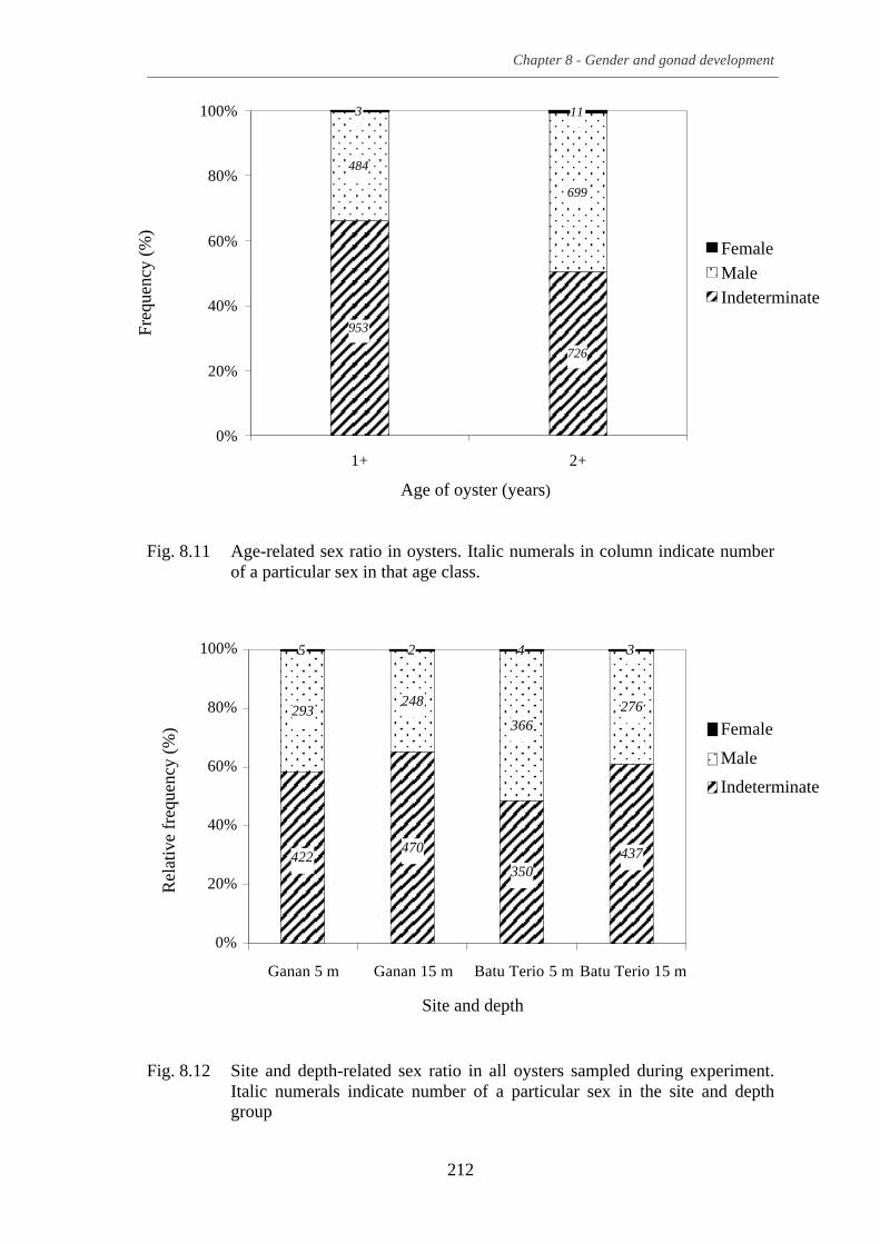
Chapter 8 - Gender and gonad development
212
Fig. 8.11 Age-related sex ratio in oysters. Italic numerals in column indicate number of a particular sex in that age class.
Fig. 8.12 Site and depth-related sex ratio in all oysters sampled during experiment. Italic numerals indicate number of a particular sex in the site and depth group
953 726
484 699
3 11
0%
20%
40%
60%
80%
100%
1+ 2+
Age of oyster (years)
Freq
uenc
y (%
)
Female Male Indeterminate
422 470
350 437
293 248
366 276
5 2 4 3
0%
20%
40%
60%
80%
100%
Ganan 5 m Ganan 15 m Batu Terio 5 m Batu Terio 15 m
Site and depth
Rel
ativ
e fr
eque
ncy
(%) Female
Male
Indeterminate

Chapter 8 - Gender and gonad development
213
8.3.3 Gonad developmental stages and GI
The combined frequencies of male and female oysters in various gonad developmental
stages are shown in Fig. 8.13. It was established that indeterminate oysters were highest
in numbers in August. Stages 1, 2 and 3 were present early in the experiment and
continued to be present throughout most of the sampling period. In contrast, Stages 4
and 5 were found mostly from December onwards, although a few were observed in
September. Oysters in Stage 6 of development were only observed in December and
January. No spawning activity was observed during sampling period. GI for each stage
is shown in Table 8.2 . In addition, the mean GI for each sampling month was plotted
and shown in Fig. 8.14. The GI rose in August and peaked in September before falling
slightly in November. In December and January, the index increased again before
falling in February.
Table 8.2 GI for the different stages of gonad development for each sampling
interval.
Gonad Stage
0 1 2 3 4 5 6
Aug 0 0.156 0.096 0.069 0.000 0.000 0.000
Sep 0 0.140 0.333 0.181 0.083 0.083 0.000
Nov 0 0.342 0.246 0.188 0.008 0.000 0.000
Dec 0 0.192 0.117 0.144 0.300 0.177 0.050
Jan 0 0.235 0.071 0.163 0.408 0.115 0.038
Feb 0 0.300 0.143 0.000 0.277 0.116 0.000

Chapter 8 - Gender and gonad development
214
Fig. 8.13 Combined gametogenic stages in male and female oysters from August 2001 to February 2002.
Fig. 8.14 Monthly mean (± SE) GI for P. maxima cultured at Ganan and Batu Terio at 5 m and 15 m depths.
0
100
200
300
400
Aug Sep Nov Dec Jan Feb
Month
Freq
uenc
y
Stages 0 1 2 3 4 5 6
0.0
0.2
0.4
0.6
0.8
1.0
1.2
Aug Sep Nov Dec Jan Feb
Month
Gon
ad in
dex

Chapter 8 - Gender and gonad development
215
8.3.4 Oyster growth
8.3.4.1 Total growth (GT)
Overall, shell length, height, thickness and wet weight of all oysters increased over the
sampling period. Total growth (GT) was positive (Table 8.3). When GT was subjected to
PCA (Appendix 1.8.3), it was found that length and height were strongly correlated to
each other (p < 0.05) and could be extracted as component 1, while thickness and
weight, though not significantly correlated, were strongly loaded to component 2 (Fig.
8.15). Together the components accounted for 73% of the variance (Table 8.4). Factor
scores were used to produce two new variables named LH (Length and height) and TW
(Thickness and weight). When the new variables were introduced into a stepwise
multiple regression analysis (Appendix 1.8.4) using binomial values for site, depth, age
and size (Appendix 1.8.2), regression of LH yielded: LH = -0.680 – 1.361 (Year 1) –
0.981 (Large) with r = 0.86, while the regression of TW = -0.508 + 1.015 (Large) with r
= 0.52.
The regression results indicate age and size accounted for variation in length and height
but did not indicate what underlying processes may be responsible for this relationship.
Shell thickness and weight appear to be less affected by size and not by age. Culture
site and depth did not have an effect in the total growth of shell length, height, thickness
and weight.
8.3.4.2 Growth rate (G30)
Growth rate of shell length, height and thickness was positive throughout the sampling
period. Weight G30 was mostly positive with the exceptions being small Year 1 oysters
cultured at a depth of 5 m at Ganan and large Year 1 oysters cultured at a depth of 15 m
in Batu Terio during August, as well as small Year 2 oysters cultured at 5 m and 15 m
in Batu Terio during February, when the G30 was negative.

Chapter 8 - Gender and gonad development
216
Table 8.3 Mean (± S.D) initial and final length, height, thickness and weight of different age and size classes of oysters, and the total average growth over the experimental period.
Large oysters Small oyster
Length (mm)
Height (mm)
Thickness
(mm)
Weight
(g)
Length (mm)
Height (mm)
Thickness
(mm)
Weight
(g) Year 1
Initial 126.76
(± 6.03)
124.13
(± 6.03)
27.22
(± 2.14)
218.12
(± 29.05)
94.23
(± 9.06)
93.98
(± 10.18)
20.58
(± 2.63)
97.87
(± 21.25)
Final 141.76
(± 11.08)
139.95
(± 10.97)
31.59
(± 2.93)
343.81
(± 47.08)
118.90
(± 15.40)
117.53
(± 12.01)
25.85
(± 4.55)
197.34
(± 52.35)
TG 15.00 15.82 4.37 125.69 24.67 23.55 5.28 99.47
Year 2
Initial 148.27
(± 6.89)
144.91
(± 8.59)
32.59
(± 2.95)
381.27
(± 41.89)
108.83
(± 11.59)
111.42
(± 10.56)
25.45
(± 2.55)
179.77
(± 40.46)
Final 154.23
(± 7.31)
152.74
(± 7.95)
35.33
(± 6.20)
483.25
(± 75.92)
121.38
(± 16.75)
123.30
(± 14.07)
28.96
(± 6.68)
252.90
(± 64.12)
TG
5.98 7.83 2.74 101.98 12.55 11.88 3.51 73.13

Chapter 8 - Gender and gonad development
217
Component 1
1.0.50.0-.5-1.0
Com
pone
nt 2
1.0
.5
0.0
-.5
-1.0
weight
thickness
height
length
Fig. 8.15 Component plot of GT parameters in rotated space.
Table 8.4 Rotated component matrix of PCA on GT of height, length, thickness and weight. Rotation method: Promax with Kaiser normalisation
Growth parameter
(GT)
Principal components Communality
1 2
Height .937 .011 0.890
Length .924 .246 0.870
Thickness -.050 .821 0.677
Weight .262 .683 0.498
Initial eigenvalues 1.83 1.12
% Variance 45.84 28.06
% Cumulative variance 45.84 73.91

Chapter 8 - Gender and gonad development
218
Table 8.5 Rotated component matrix of PCA on G30 of height, length, thickness and weight. Rotation method: Promax with Kaiser normalisation.
PCA of G30 (Appendix 8.5) resulted in one component being extracted that explained
78% of the variance in the factors (Table 8.5). The factor scores for the principal
component were used to plot changes in G30 and to compare difference in growth of
oysters. As only one component was extracted, G30 of shell length, height, thickness
and weight was grouped and discussed as a single entity.
8.3.4.2 (a) Age, size and temporal effect
When an ANOVA (Appendix 1.8.6) was performed on G30 as the dependent variable,
the results indicated that age, size and sampling time had a significant effect on growth
rate (Age: F(1,4) = 78.92, p < 0.05; Size: F(1,4) = 47.73, p < 0.05; Sampling: F(4,4) = 54.8,
p < 0.05). There was significant interaction between age of oyster and time of sampling
(F(4,4) = 27.81, p < 0.05). Post-hoc test confirmed that G30 for September differed from
all the other months.
With few exceptions, G30 of Year 1 oysters were consistently higher than Year 2 oysters
(Fig. 8.16). For both age classes, smaller oysters appear to have higher G30 than larger
Growth parameter
(G30)
Principal component
Communality
1
Height .942 .882
Length .939 .887
Thickness .925 .522
Weight .723 .856
Initial eigenvalues 3.14
% Variance 78.63
% Cumulative variance 78.63

Chapter 8 - Gender and gonad development
219
oysters. The temporal variation in G30 could be observed with maximum growth rates
occurring in September for both age and size groups and minimum growth occurring in
November (Fig. 8.16 and Fig. 8.17).
8.3.4.2 (b) Spatial effect
While G30 was not significantly different between oysters cultured at Ganan and Batu
Terio and between the two depths when tested with an ANOVA (Appendix 1.8.6), the
average G30 of oysters cultured at 5 m was higher than oysters cultured at 15 m at both
sites in December and January. When G30 scores were plotted as a function of site and
depth, growth rate for both sites were observed to peak in September (Fig. 8.17).
8.3.5 Condition index
CI for large and small Year 1 and Year 2 oysters peaked at the start of the experiment in
August then dropped sharply in September, before gradually reaching a second peak in
December (Fig. 8.16). Temporal changes in CI appeared to be reflected by inverse
changes in monthly instantaneous growth rates - the decline in CI of oysters in
September coincided with a peak in the monthly instantaneous growth, while the rise of
the index in December was inversely reflected in a drop in monthly instantaneous
growth rate during that month.
According to linear regression (Appendix 1.8.7) of log10 CI and environmental data,
water temperature, salinity, pH, rainfall, SPM, POM, chlorophyll a, b, and c explained
only 18% (p < 0.05) of the variation in the sampled oysters. Based on standardised
partial regression coefficients (!) that indicate the relative importance of independent
factors upon the dependent variable (Zar, 1984), chlorophyll a (! = -1.04) chlorophyll b
(! = -0.73), chlorophyll c (! = 1.77), water temperature (! = 0.47) and salinity (! =
0.34) had the greatest influence on CI. Pearson’s correlation analysis (Appendix 1.8.7)
revealed that CI was correlated (p < 0.05) to water temperature (r2 = 0.204) and salinity
(r2 = 0.243) but not to the other environmental variables.

Chapter 8 - Gender and gonad development
220
Fig. 8.16 Comparison between monthly G30 score (obtained by PCA of shell length, height, thickness and wet weight of oysters) and CI of oysters from two age and size classes.
-1.0
0.0
1.0
2.0
3.0 Fa
ctor
sco
re fo
r G30
100
150
200
250
300
Aug Sep Nov Dec Jan Feb
Date
Con
ditio
n in
dex
Year 1 Small Year 2 Large Year 2 Small
Year 1 Large
Year 1 Small Year 2 Large Year 2 Small
Year 1 Large
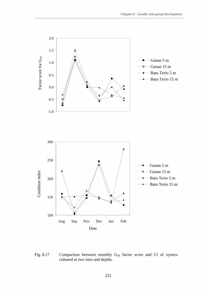
Chapter 8 - Gender and gonad development
221
Fig. 8.17 Comparison between monthly G30 factor score and CI of oysters cultured at two sites and depths.
-1.0
-0.5
0.0
0.5
1.0
1.5
2.0
100
150
200
250
300
Aug Sep Nov Dec Jan Feb
Date
Con
ditio
n in
dex
Fact
or s
core
for G
30
Ganan 5 m Ganan 15 m Batu Terio 5 m Batu Terio 15 m
Ganan 5 m Ganan 15 m Batu Terio 5 m Batu Terio 15 m

Chapter 8 - Gender and gonad development
222
8.3.6 Environmental parameters
As environmental parameters were presented in detail in Chapter 4, changes in each
parameter will not be repeated in this Chapter. However, as Chapter 4 explored
environmental parameters from three sites and two depths over a 20 months period
while in this study, two sites were compared and the period for the experiment was
seven months, environmental data from the relevant time-frame were extracted from the
overall data set to perform analyses. Environmental descriptors for the duration of this
experiment at Ganan and Batu Terio are summarised in Table 8.6.
8.3.7 Relationship between sex, size and environmental parameters
The relationships between sex and size (as measured by length, height, thickness and
weight), and sex and various environmental parameters were investigated using
discriminant analysis.
8.3.7.1 Sex, size and weight
Mean length, height, thickness and wet weight of indeterminate, male and female
oysters are given in Table 8.7. The mean length, height, thickness and weight of female
oysters were greater than that of male oysters which were in turn larger than
indeterminate oysters.
As there were three groups (indeterminate, male and female) to be classified, two
discriminant functions were produced consisting of two canonical or discriminant
variables (DV) (Appendix 1.8.10). Stepwise analysis established that weight, length and
height were significant in separating the categories. DV1 appeared to distinguish
indeterminate oysters from males and females by weight, while DV2 appeared to
separate males from indeterminate oysters based on length (Fig. 8.18). However, there
appeared to be a high degree of overlap between the different groups. In the
classification matrix, indeterminate oysters were classified correctly 80.3% of the time
while the number of oysters properly categorised as males and females were 42.8% and
35.7%, respectively.

Chapter 8 - Gender and gonad development
223
Table 8.6 Means (± SD) of various environmental parameters at Ganan and Batu Terio at 5 m and 15 m depths.
Site
Month
Temperature (°C)
Salinity
(‰)
PH
SPM
(g L-1)
POM (g L-1)
Chlorophyll a
(g L-1)
Chlorophyll b
(g L-1)
Chlorophyll c
(g L-1)
Ganan Aug 27.58 (0.22) 34.4 (0.9) 7.4 (0.1) 0.0340 (0.0055) 0.0140 (0.0055) 0.8238 (0.8754) 1.2511 (1.3957) 3.3688 (3.7631) 5 m Sep 27.73 (0.32) 34.0 (0.8) 7.5 (0.1) 0.3150 (0.0060) 0.0115 (0.0087) 0.3988 (0.1674) 0.5573 (0.2988) 1.5390 (0.7939) Nov 28.18 (0.37) 35.0 (0.8) 7.6 (0.1) 0.0350 (0.0058) 0.0075 (0.0050) 0.7867 (0.3039) 1.0045 (0.4319) 2.7434 (1.2078) Dec 29.21 (0.48) 35.0 (0.0) 7.7 (0.1) 0.0340 (0.0055) 0.0100 (0.0071) 0.2717 (0.3851) 0.4503 (0.6279) 1.2189 (1.8099) Jan 28.71 (0.24) 34.5 (0.6) 8.0 (0.0) 0.0225 (0.0050) 0.0075 (0.0050) 0.0219 (0.0155) 0.1375 (0.0750) 0.1188 (0.1048) Feb 28.50 (0.29) 35.0 (0.0) 8.0 (0.1) 0.0300 (0.0082) 0.0050 (0.0058) 0.0063 (0.0078) 0.0438 (0.0375) 0.0250 (0.0540) Ganan Aug 28.19 (0.17) 34.8 (0.8) 7.6 (0.1) 0.0360 (0.0055) 0.0060 (0.0055) 0.8700 (0.2405) 1.2439 (0.2877) 3.4218 (0.8117) 15 m Sep 28.35 (0.24) 34.0 (0.8) 7.7 (0.1) 0.0350 (0.0058) 0.0050 (0.0058) 0.2546 (0.2233) 0.3261 (0.3439) 0.9534 (0.9287) Nov 28.80 (0.33) 35.0 (0.0) 7.7 (0.1) 0.0300 (0.0082) 0.0100 (0.0082) 0.5999 (0.5094) 0.8911 (0.7846) 2.5123 (2.1948) Dec 29.07 (0.29) 35.0 (0.0) 7.8 (0.1) 0.0300 (0.0000) 0.0040 (0.0055) 0.2101 (0.2639) 0.3534 (0.3591) 0.8275 (1.3317) Jan 28.70 (0.14) 35.0 (0.0) 8.0 (0.0) 0.0275 (0.0096) 0.0050 (0.0058) 0.0194 (0.0083) 0.1188 (0.0375) 0.1000 (0.0456) Feb 28.66 (0.18) 35.0 (0.0) 8.0 (0.0) 0.0350 (0.0058) 0.0100 (0.0000) 0.0013 (0.0127) 0.0188 (0.0688) 0.0250 (0.0957) Batu Terio Aug 28.56 (0.19) 34.2 (1.1) 7.6 (0.2) 0.0360 (0.0089) 0.0140 (0.0114) 0.4549 (0.2497 0.6324 (0.4046) 1.8248 (1.2168) 5 m Sep 28.83 (0.19) 33.5 (0.6) 7.6 (0.2) 0.0325 (0.0050) 0.0075 (0.0050) 0.3271 (0.2413) 0.4555 (0.3135) 1.2971 (0.9456) Nov 29.34 (0.32) 34.5 (0.6) 7.8 (0.2) 0.0300 (0.0115) 0.0050 (0.0058) 0.3988 (0.1674) 0.5573 (0.2988) 1.5390 (0.7939) Dec 29.37 (0.35) 35.0 (0.0) 7.7 (0.1) 0.0300 (0.0071) 0.0060 (0.0089) 0.4135 (0.4356) 0.6131 (0.6912) 1.7499 (2.1337) Jan 28.94 (0.22) 34.8 (0.5) 8.0 (0.0) 0.0325 (0.0050) 0.0075 (0.0050) 0.0006 (0.0047) 0.0313 (0.0239) 0.0063 (0.0427) Feb 29.13 (0.22) 35.0 (0.0) 8.0 (0.0) 0.0275 (0.0050) 0.0075 (0.0050) 0.0063 (0.0060) 0.1438 (0.0375) 0.0250 (0.0456) Batu Terio Aug 28.15 (0.31) 34.0 (1.4) 7.6 (0.2) 0.0320 (0.0084) 0.0140 (0.0089) 0.4885 (0.2573) 0.7684 (0.3341) 2.0426 (0.8662) 15 m Sep 28.35 (0.41) 33.3 (1.0) 7.5 (0.2) 0.0325 (0.0096) 0.0075 (0.0050) 0.1666 (0.1217) 0.1701 (0.2815) 0.6535 (0.7003) Nov 28.80 (0.45) 34.5 (0.6) 7.8 (0.2) 0.0325 (0.0050) 0.0100 (0.0000) 0.2999 (0.1692) 0.2913 (0.3958) 0.9045 (0.9338) Dec 29.22 (0.41) 35 (0.0) 7.7 (0.1) 0.0320 (0.0045) 0.0040 (0.0089) 0.2099 (0.2750) 0.3230 (0.3534) 0.8142 (1.1843) Jan 28.78 (0.31) 34.8 (0.5) 8.0 (0.0) 0.0300 (0.0082) 0.0025 (0.0050) 0.0050 (0.0061) 0.0500 (0.0289) 0.0250 (0.0354) Feb 28.74 (0.18) 35.0 (0.0) 8.0 (0.0) 0.0275 (0.0096) 0.0050 (0.0058) 0.0144 (0.0085) 0.0813 (0.0427) 0.0750 (0.0677)

Chapter 8 - Gender and gonad development
224
Table 8.7 Mean (± SD) length, height, thickness and weight of indeterminate, male and female oysters in mm.
Fig. 8.18 Scatter plot showing sex groupings of oysters by two discriminant variables.
Sex
Indeterminate
Male
Female
Length 119.9 (20.1) 137.5 (17.1) 138.6 (19.8)
Height 119.3 (19.0) 136.3 (16.5) 140.5 (14.9)
Thickness 26.9 (5.4) 30.7 (4.7) 32.4 (3.8)
Weight 222.1 (105.8) 326.0 (112.4) 367.6 (97.4)
-8
-6
-4
-2
0
2
4
6
8
10
-4 -3 -2 -1 0 1 2 3 4
Canonical variable 1
Can
onic
al v
aria
ble
2
.
Indeterminate
Male
Female

Chapter 8 - Gender and gonad development
225
The correlation (r) of a particular variable to the discriminant functions may be used to
determine the relative importance of the variable (Table 8.8). DV1 separated
indeterminate oysters from males and females based on weight (r = 0.967), height (r =
0.948) and length (r = 0.933) while DV2 separated indeterminate oysters from males
based mainly on length (r = 0.339). Thickness did not appear to be an important factor
in discriminating between the sexes.
Although the analysis was significant in separating between the groups using the Wilks
Lambda statistic (Weight: F (2,2873) = 324.2, p < 0.05; Length: F (4,5744) = 162.1, p <
0.05; Height: F (6,5742) = 110.0, p < 0.05), size and weight were not reliable predictors of
sex because of the low percentages of correctly classified cases as well the overlap in
the scatter plot.
8.3.7.2 Sex and environmental parameters
There was an inverse correlation (Appendix 1.8.11) between the number of
indeterminate oysters and pH (r2 = -0.209, p < 0.05), water temperature (r2 = -0.261, p <
0.05) and rainfall (r2 = -0.261, p < 0.05) over the sampling period. A positive
correlation was also observed between the number of male oysters and pH (r2= 0.204, p
< 0.05), water temperature (r2= 0.261, p < 0.05) and rainfall (r2= 0.217, p < 0.05). No
correlation was found between female oyster numbers and environmental parameters.
Graphical representation showed that as rainfall, water temperature and pH increased
from August to December, there was a concomitant increase in the number of male
oysters and a decrease in the number of indeterminate oysters (Fig. 8.23). However,
when rainfall and temperature decreased from December to February, a decrease of the
same magnitude was not observed in male oysters. The change in male and
indeterminate numbers was relatively small from December to February.
While it appeared that pH, temperature and rainfall were significantly correlated to the
number of indeterminate and male oysters, the correlations were relatively weak and
did not fully account for the variation in the number of male and indeterminate oyster
adequately.

Chapter 8 - Gender and gonad development
226
Table 8.8 Coefficients of discriminant functions and correlation (r) of variables to the discriminant variables (DV).
Variable
DV1
DV2
Correlation to
DV1
Correlation to
DV2
Weight 0.479 -1.736 0.967 -0.210
Height 0.315 -0.083 0.948 0.045
Length 0.255 1.884 0.933 0.339
Thicknessa 0.714 -0.084
a. Not used in analysis

Chapter 8 - Gender and gonad development
227
0
100
200
300
400
0
100
200
300
400
Indeterminate Male rainfall
0
100
200
300
400
28
29
29
30
0
100
200
300
400
Aug Sep Nov Dec Jan Feb
Date
7.4
7.6
7.8
8.0
8.2
No
of o
yste
rs
Rai
nfal
l (m
m)
Tem
pera
ture
(°C
) pH
Fig. 8.19 Relationship between the number of indeterminate and male oysters
and rainfall, water temperature and pH.

Chapter 8 - Gender and gonad development
228
8.4 Discussion
The reproductive cycle in bivalve oysters involves several stages: growth and ripening
of gametes, spawning and gonad redevelopment (Gosling, 2003). This study attempts to
assess the course of the reproductive cycle in P. maxima through gross visual
examination of the gonads. While this method does not provide detailed information on
the development of gametes like that provided by histological or biopsy methods
(Barber and Blake, 1991), it does offer a simple and quick method to estimate overall
gonadal development in the field where access to more advanced equipment and
technique are limited. It also has the advantage of not requiring the sacrifice of an
animal.
Macroscopic investigation of gonads and comparison to histological data in this study
support previous reports that gonad colour and appearance may be used to determine
sex and stage of development in P. maxima (Rose et al., 1986). The difference between
the pale creamy patchiness in the digestive diverticula of male oysters, the bright
yellow-orange patchiness in female oysters and the clear translucence of indeterminate
oysters was very conspicuous in this species of pearl oyster. This fundamental
difference in the colour and the area occupied by the developing gametes made it
possible to distinguish between the gender and various stages of development of P.
maxima oysters with relative ease, as demonstrated when visual observations were
confirmed by histology (Appendix C). While gonad colour may be used to distinguish
between sexes in P. maxima and P. albina (Tranter, 1958a), it is not a reliable criterion
in other species of pearl oysters. For example, sex in P. imbricata could be
distinguished by colour only in the later stages of development (O’Connor and Lawler,
2004b; Choi and Chang, 2003; Behzadi et. al., 1997; Velayudhan and Gandhi, 1987;
Tranter, 1959) while histological examination is often required to determine sex in P.
mazatlanica (Saucedo and Monteforte, 1997a; Garcia-Dominguez et. al., 1996) and P.
margaritifera (Tranter, 1958d).
In this study, gametogenesis commenced immediately after pre-conditioned oysters
were placed at experimental sites, as shown by the number of sexually distinct oysters
observed at the first month of sampling. Proportion of indeterminate oysters fell to 77%
from an initial 100% and oysters with distinct sex were observed as spermatogenesis

Chapter 8 - Gender and gonad development
229
progressed, followed by oogenesis in a small number of oysters. In November, the
proportion of indeterminate oysters was at its lowest (50%) after which the percentage
of indeterminate oysters began to increase again. The percentage of indeterminate
oysters observed was always inversely proportional to the percentage of sexually
distinct oysters as oysters went through the gonadal cycle. The gonadal cycle began
from an inactive state (forced by pre-conditioning in an unfavourable environment),
progressed towards gonad maturity and finally culminated in a spawning event in
September – November and again towards the end of the experiment in February. The
subsequent increase in indeterminate oysters observed after those months represented
spent oysters that had discharged gametes during spawning. Spawning was likely partial
as male and female oysters with ripe gonads continued to be observed after November.
Observation on the proportion of inactive and sexually mature oysters within a
population of oysters could be used to interpret the gametogenic cycle of cultured P.
maxima.
The timing of the gametogenic cycle was supported by observations of changes in the
gonad index (GI). As GI increases during gametogenesis and decreases during
spawning (Gosling, 2003), results could be interpreted as follows: gametogenesis
commenced from August, followed by a partial spawning in September – November. It
would appear that not all gametes were released, as the drop in the index was slight. In
the following months, gametogenesis continued and resulted in a second spawning in
February when the GI decreased for the second time.
Observation of gonad stages was consistent in supporting the findings that there was
bimodal spawning in September - November and January - February. The number of
Stage 0 oysters observed decreased progressively from August until November matched
by a corresponding increase in Stage 1 and 2 oysters, indicative of the oysters
undergoing the developing stage of gametogenesis when production of gametes was on
the rise. A rise in the number of Stage 0 oysters was observed in December together
with a corresponding fall in Stage 1 oysters. This was seen as oysters having spawned
prior to the November sampling with the expulsion of gametes giving rise to the large
number of Stage 0 spent oysters. Ripe oysters (Stages 4, 5 and 6) were not observed in
November but were present in most of the other months, thus confirming that oysters
had spawned before the November sampling. The number of Stage 1 plus oysters

Chapter 8 - Gender and gonad development
230
increased until February, leading to the conclusion that a second stage of gametogenesis
occurred to be followed by a second spawning.
Previous literature indicates that mature P. maxima oysters undergo an annual
reproductive cycle which appear to vary in timing and duration according to location
(Wada, 1953b; Minaur, 1969; Rose et. al., 1990). This has also been reported in other
pearl oysters (Wada et al., 1995; O’Connor, 2002; Choi and Chang, 2003). Differences
in the reproductive cycle of bivalves from the same species are thought to be due to
critical water temperatures being achieved at different latitudinal ranges and at different
times (Giese, 1959; Giese and Pearse, 1974) as water temperature has been reported to
affect the onset of gametogenesis in pearl oysters (Araya-Nuñes et. al., 1991; Behzadi
et. al., 1997; Saucedo and Monteforte, 1997a; O’Connor, 2002; Choi and Chang, 2003;
O’Connor and Lawler, 2004b). For example, P. maxima populations in Queensland
were observed to have two breeding peaks, October – November and February – March
(Wada, 1953b; Minaur, 1969) while P. maxima in Western Australia were observed to
breed from September to April with peaks at either ends (Rose et. al., 1990).
Table 8.9 Spawning months of various species of pearl oysters found in different localities.
Pearl oyster species Locality Spawning months References P. maxima Queensland,
Australia October - November February - March
Wada, 1953b Minaur, 1969
Western Australia September – April Rose et. al., 1990
West Papua, Indonesia
September – November January - February
This study
P. fucata martensii Japan Continuous, with major peak in winter and minor peak in summer
Wada et. al., 1995
Korea April – August, with peak in June – July
Choi and Chang, 2003
P. albino sugillata New South Wales, Australia
Continuous, with peaks in Oct, Mar, Jan and April
O’Connor, 2002

Chapter 8 - Gender and gonad development
231
Rose (1990) hypothesized that the difference in the timing was most likely due to the
variation in surface water temperature at the two latitudes as P. maxima studied in
Western Australia was approximately 7 to 11 degrees south from the Queensland
populations and exposed to a lower minimum water temperature (18°C). Aljui Bay is
situated close to the equator (Latitude 00° 11’ S) and water temperature did not go
below 27.6°C in this study. However, despite the mean water temperature at Aljui Bay
being higher than the Australian sites, the timing for the reproductive cycles in P.
maxima at Aljui Bay and Western Australia appear to occur around the same time of the
year. It is likely that other factors, biological and environmental, also exert an influence
on the gonadal cycle of P. maxima besides water temperature.
Visual inspection of gonad conditions has its limitations, as it was difficult to ascertain
if indeterminate oysters were in an inactive or spent stage since the stages often
overlapped. However, given what is known about the gametogenic cycle of pearl
oysters in general (Rose et. al., 1990; Garcia-Dominguez et. al., 1996; Saucedo and
Monteforte, 1997a; Choi and Chang, 2003; O’Connor and Lawler, 2004b), it is possible
to approximate what state Stage 0 oysters were at during the experiment. Another
disadvantage of visual examination is that classification tends to be subjective (Gosling,
2003). The problem can however be overcome in a farm situation if specifically trained
workers were delegated the task of estimating gonad condition in preparation for
artificial propagation. The advantage of not sacrificing a valuable pearl oyster
outweighs the potential for possible errors in classifying gonad condition in cultured P.
maxima.
GI estimated the proportion of developing, ripe, spawning and spent individuals by
classifying sexual stages of the whole population of experimental oysters. CI, on the
other hand, estimated the current metabolic and reproductive status of individual pearl
oyster. A decrease in CI indicates a decrease in tissue weight of oysters likely caused
when a major biological effort has been expended. The probable cause of this is loss of
gonad tissue due to a recent spawning. From the results, low CI in September and
January (Fig. 8.16 and Fig. 8.17) indicate that oysters spawned around the period and is
consistent with other results obtained by visual examination of gonads. Condition
indices assess physiological activity such as growth, reproduction or secretion in
animals (Lucas and Beninger, 1985) and can indicate the nutritive state of the animal

Chapter 8 - Gender and gonad development
232
(Brown and Hartwick, 1988c; Littlewood and Gordon, 1988). While CI is accurate in
estimating the physiological state of an oyster, it represents only an individual. A larger
sample is required to estimate with more accuracy the reproductive state of a population
of oysters. Unfortunately, this is not economically viable in a farming situation. In this
regard, GI is preferable as it has the advantage of not requiring the destruction of the
animal.
Pearl oysters are protandric hermaphrodites and can reverse sex several times during
their lifetimes (Galstoff, 1950; Wada, 1953a, 1953b; Chellam, 1987; Saucedo and
Monteforte, 1997a; Vite-García and Saucedo, 2008). Pearl oysters in a natural
population achieve a sex ratio of 1:1 with increasing age and size (Wada, 1953; Gervis
and Sims, 1992). However, there have been reports that oysters in close proximity often
result in a higher proportion of male in the population (Burkenroad, 1931; Menzel,
1951; Buroker, 1983; Taylor, 1999; Walker and Power, 2001; Kimani and Mavuti,
2002; Saucedo et. al., 2002a, 2002b). This was shown to be the case here as the sex
ratio of female to male was an overwhelming 0.01:1. Similarly, Saucedo and
Monteforte (1997a) reported a strong male bias in small P. mazatlanica in Mexico, with
a female to male sex ratio of 0.12:1, and increasing to 0.38:1 as oysters grew larger.
Saucedo et al., (2002b) also described a 0.35:1 female to male ratio in P. mazatlanica
obtained from cultured conditions, but indicated that females outnumbered males in the
wild. It has been proposed that the predominance of maleness is an indication of
ambient stress and/or unsuitable culture condition with overcrowding playing a key role
in greater expression of maleness (Saucedo and Southgate, 2008). Morton (1991)
hypothesised that a male bias in juvenile bivalves allows for a more efficient allocation
of resources into growth. Male gamete production is more cost effective since juvenile
mortality in an unfavourable environment may be higher than for larger individuals.
Older females, on the other hand with lower growth rates may divert more energy into
ova production and with reduced mortality enhance the potential for fertilisation. The
funnelling of energy into survival and growth by a protandrist in its male phase before
taking advantage of the energy saved to become female, is an elaboration of the “size-
advantage model” (Ghiselin, 1969), a theory to explain the evolution of protandry. This
model predicts that when the reproductive success (RS, or number of viable offspring
produced) of males are less sensitive to size and age than the RS of females, a
protandric individual gains a reproductive advantage.

Chapter 8 - Gender and gonad development
233
Sex change is reversible in several species of oysters and thought to be caused by
changing environmental condition and stress (Cahn, 1949; Tranter, 1958a, b, c, d, 1959;
Chellam 1987; Rose et. al., 1990). Until recently, the prevailing view was that sex in
various species of oysters was predominantly determined by environmental factors such
as water temperature, acute water temperature changes (such as in an El Niño or La
Niña event), salinity, nutritive conditions or food availability (Coe, 1943; Rao, 1956) or
that hormone might be the major controlling mechanism (Kennedy, 1983; Thompson et
al., 1996). Results from this study showed that there was a correlation between pH,
water temperature and rainfall and the number of male oysters observed. As rainfall,
water temperature and pH increased from August to December, there was a
concomitant increase in the number of male oysters. pH can significantly alter the
physiology of marine invertebrates by having a synergistic effects with other
environmental factors such as elevated temperatures (O’Donnell et al., 2009), while
rainfall could change the pH of seawater. That water temperature was correlated to
spermatogenesis is not surprising, as it has been widely reported to affect
gametogenesis in other pearl oysters (Wada, 1953b; Minaur, 1969; Rose et al., 1990;
Araya-Nuñes et. al., 1991; Behzadi et. al., 1997; Saucedo and Monteforte, 1997a;
O’Connor, 2002; Choi and Chang, 2003; O’Connor and Lawler, 2004b). While there
was positive correlation between environmental parameters and the expression of
maleness, the correlations were relatively weak and did not fully account for the
variation in the number of male oyster adequately. The occurrence of female oysters did
not correlate to any environmental parameters. Given the persistently low number of
female oysters observed in this study, the absence of any correlation between
environmental parameters and number of female oysters should be interpreted with
caution. The implications of these results are that environmental parameters affect the
onset of spermatogenesis in P. maxima to a certain extent, but oogenesis is less
governed by environmental parameters. Other factors, for example, biological or
hormonal, are likely to play important roles in controlling gametogenesis.
Besides environmental parameters, a genetic basis of sex differentiation has been
proposed by a number of authors. Tranter (1958c) hypothesized that a “weak hereditary
sex-determining mechanism” may be responsible for sex change in P. albina, and more
recently Guo et al. (1998) showed that sex in the rock oyster Crassostrea gigas was
determined by a single gene locus with a dominant maleness allele and an allele for

Chapter 8 - Gender and gonad development
234
protandric femaleness, and other genes and/or environmental factors such as
temperature may regulate the rate of sex change. Bacci (1965) suggested that the
duration of the male or female phase in oysters may result from simple Mendelian
segregation of multiple sex genes whose action is additive. Haley (1975) proposed a
three loci model for sex determination in the American oyster, C. virginica, with each
locus segregating two additive alleles, m for maleness and f for femaleness, with the
m:f ratio determining sex. Arnoud-Haond et al., (2003) compared the geographical
distribution of genetic variability at mitochondrial and nuclear loci among natural
populations of P. mazatlanica in the tropical American Pacific coast and showed
evidence for male-biased effective sex ratio. While there is probably a genetic basis for
sex differentiation in P. maxima, it is likely that gene expression is mediated by external
factors such as environmental parameters, with both endogenous and exogenous factors
acting in concert to determine sex differentiation.
While the reproductive system in pearl oysters is relatively simple, consisting of
branching tubules with an epithelial lining from which gametes bud off and are shed
through an exhalant opening in the mantle (Gosling, 2003; Southgate and Lucas, 2008),
gametogenesis is a complex process which is controlled by a multitude of factors
encompassing biological, physical and chemical parameters. In this study, attempts to
partition the relative influence of the various factors using statistical procedures
produced outcomes, which can be interpreted in a meaningful biological context.
Results showed that that spermatogenesis and oogenesis in P. maxima cultured at Aljui
Bay were influenced by temporal (months of sampling as discussed earlier) and
biological factors (age and size of oysters) but not by spatial factors (site or depth of
culture). Results indicated that more males were found within faster growing oysters
from a younger age (Year 1 Large) than slower growing oysters from an older age
(Year 2 Small). Similarly, femaleness was also size-related. The implication for this is
that size, and not age was more important in the expression of sex in P. maxima.
Furthermore, discriminant analysis showed that indeterminate oysters could be
separated from males and females based on wet weight (r = 0.967), shell height (r =
0.948) and shell length (r = 0.933) and indeterminate oysters could be distinguished
from males based mainly on shell length (r = 0.339) while shell thickness was not
important in discriminating between the sexes. In a farm situation, this information
could be utilised by selecting and maintaining oysters with greater shell length or shell
Chapter 8 - Gender and gonad development
235
height, regardless of age, for breeding stock and using smaller oysters for pearl seeding.
By selecting larger oysters as broodstock, the likelihood of male and female expression
is increased.
The overwhelming bias towards male oysters in this experiment may be due to other
reasons besides those discussed. For instance, the duration of this experiment may not
have been sufficiently long enough to enable conversion to the female state. Secondly,
the majority of oysters used in this experiment fell between the 100 mm to 160 mm size
range. Sex ratio in P. maxima from Western Australia was reported to approach parity
only when oysters become larger and females reach a dorso-ventral measurement of
170 mm (Hart and Joll, 2006). Due to the scarcity of P. maxima with shell lengths >
170 mm, (only 12 out of the 480 oysters sampled had shell length > 170 mm), this
theory could not be assessed in the study. However, given what is know about sex
reversal in general in P. maxima, it is likely that the f:m sex ratio would be closer to
parity if oysters from a larger size range was used in any future studies.
In summary, this study showed that gametogenesis in cultured P. maxima in Aljui Bay
occurred between August to February, with spawning occurring twice during that
period; once in October/November and again in February. Sex ratio was
overwhelmingly biased towards maleness, and varied temporally for the duration of the
experiment. There was no difference in sex ratio between oysters cultured at different
sites and different depths. The expression of maleness was weakly correlated to water
temperature, pH and rainfall, while there was no correlation between femaleness and
environmental descriptors. Size, and not age, was more important in determining the
sex of P. maxima in this study.

Chapter 9 – General Discussion
236
CHAPTER 9
General Discussion
9.1 Background to the study
The culture of P. maxima at P. T. Cendana encompasses the entire life cycle of oysters,
starting with artificial propagation of broodstock to produce larvae, followed by grow-
out of oysters from juvenile to adulthood in the ocean, and ending with using oysters to
produce pearls or as broodstock. Hatchery techniques have improved in recent years and
reliable production of P. maxima larvae in the hatchery is a feature of most pearl farms.
However, the ocean grow-out phase of P. maxima culture is still frequently subjected to
various uncertainties including slow growth of animals (Traithong et al., 1997), high
mortalities (Wu et al., 2003b) and fouling and predation particularly in juvenile oysters
(Gervis and Sims, 1992). This is due to the difficulty of creating a controlled growing
environment out in the open ocean. However, it has been previously reported in other
studies that growth variability in a population of molluscs living in the same locality has
been reported to be related to differences in the microenvironments (Wilbur and Owen,
1964). Therefore, the selection of a particular culture site or culture depth within a farm
is an indirect method of exerting control over the growth environment of cultured pearl
oysters. Understanding how spatial difference affect growth and survival of P. maxima
at different stages of growth would serve to assist management in refining grow-out
techniques for optimal production of oysters.
This thesis aimed to address various growth aspects of farming P. maxima in a
commercial farm in Indonesia with special emphasis on the influence of the
environment, as bivalve growth is affected by a complex combination of biological and
environmental factors.

Chapter 9 – General Discussion
237
9.2 Major findings of this study
The major findings in this study were:
1. Seawater parameters in the P. maxima growing area of Aljui Bay were not
homogenous and environmental descriptors varied spatially between sites and
depths, as well as temporally throughout the year.
2. Growth of P. maxima was affected by the age of the oysters, with growth slowing
down with increasing age. Growth was also influenced by site and depth of
culture. Further results showed differences in spatial growth rates was linked to
the physico-chemical profile of the culture micro-environment, with variation in
somatic growth of P. maxima governed by varying levels of pH, salinity and
chlorophyll, while variation in gonad growth was influenced by variations in pH,
SPM, POM and water temperature.
3. The Special VBGF was the mathematical model that best described the growth of
P. maxima cultured in Aljui Bay.
4. Biofouling quantity and diversity affected growth of medium and small oysters.
The spatial and temporal variation in quantity and diversity of six classes of
biofouling was in turn affected by various environmental parameters, with
chlorophyll levels, pH and salinity having a greater affect on biofouling settlement
than SPM, POM and seawater temperature.
5. Gametogenesis in cultured P. maxima in Aljui Bay occurred between August to
February, with spawning occurring twice during that period; once in
October/November and again in February. Sex ratio in cultured P. maxima was
overwhelmingly biased towards maleness, with no spatial difference in sex ratio
between oysters cultured at various sites and depths. The expression of maleness
was weakly correlated to water temperature, pH and rainfall, while there was no
correlation between femaleness and environmental descriptors. Size, and not age,
was more important in determining the sex of P. maxima.

Chapter 9 – General Discussion
238
9.3 Implications of these findings
1. The heterogeneous nature of environmental parameters at various sites around
Aljui Bay means it is possible to culture P. maxima in various culture
microenvironments within a farm, thus allowing culturist some level of control
over the grow-out environment. Given the importance of environmental
parameters in many aspects of P. maxima farming, it is recommended that some
level of environmental monitoring be conducted as part of routine farming
protocol. This is to ensure that any changes in the physico-chemical profile of a
particular growing site are detected and grow-out management be adjusted
accordingly. Identification of potential new sites should also take into
consideration the environmental profile of the microenvironment.
2. It was found that culturing young P. maxima at the more favourable depth of 5 m
favour faster somatic growth and shorten the time it takes for pearl oysters to
reach operable size. The use of less rope for suspending oysters at 5 m reduces
entanglement and saves on the cost of culture material. Conversely, as the quality
of the resulting pearls has been reported to depend on slower growth and nacreous
deposition (Wada, 1973; Pouvreau and Prasil, 2001), this can be achieved by
suspending P. maxima at a depth of 15 m or greater during the pearl culture phase.
Results of this study showed that P. maxima aged 1.5 to 3.5 years old grown at
Batu Terio had the lowest survival rate. In light of this data, Ganan and Manselo
should be selected for the culture of younger P. maxima in Aljui Bay, and Batu
Terio be utilised for the culture of older and larger oysters.
3. Estimation of growth rate K, length at age t Lt and asymptotic size L! using the
VBGF showed that in the first two years of culture, the best site for grow-out
would be Manselo at a depth of 5 m when fast growth, high survival and larger
asymptotic size are essential to produce large numbers of oysters for grafting.
Oysters grown at Ganan and at a depth of 15 m had lower K values and would be
suitable to condition oysters prior to grafting and also for pearl grow-out.
4. Information on the effects of age, site, depth and month of sampling on quantity
and diversity of biofouling may be utilised in management of biofouling control in

Chapter 9 – General Discussion
239
P. maxima culture. Cleaning approximately every 4 weeks was effective in
keeping biofouling down, without detrimental effect to oysters. However, the
scheduling of a cleaning regime according to oyster size may be of further benefit
to ensure valuable resources are not wasted in superfluous cleaning, as smaller
oysters require less cleaning than larger oysters. Bivalves contributed the greatest
proportion of biofouling by weight - it would be judicious to avoid sites with high
bivalve infestations that could potentially add excess weight to the suspended
culture systems and impair floatation. A preliminary survey of the benthic
composition at prospective sites would provide information on potential
biofouling at those sites, as the settlement of biofouling organism is often a
reflection of the predominant species composition of the surrounding habitat.
5. Preparation of oysters for spawning at Aljui Bay should take place in August,
when gametogenesis commences. By selecting larger oysters as broodstock, the
likelihood of male and female expression is increased, as maleness and
femaleness in P. maxima are size-related. Indeterminate oysters could be
separated from males and females based on wet weight (r = 0.967), shell height (r
= 0.948) and shell length (r = 0.933) and indeterminate oysters could be
distinguished from males based mainly on shell length (r = 0.339). In a farm
situation, selecting and maintaining oysters with greater shell length or shell
height, regardless of age for breeding stock and using smaller oysters for pearl
seeding is recommended.
Table 9.1 summarises the various stages of grow-out of P. maxima at Aljui Bay and
shows how the results from this study may be used to assist in the management of
farming P. maxima. In summary, this research presented new data on growth of
different age classes of P. maxima cultured in a farm situation in Indonesia. It has added
to our knowledge the importance of various environmental factors and biofouling on
somatic and gonadal growth of P. maxima. This information can be utilised to improve
farming management practices through judicious selection of future culture sites. It is
hoped that this will form a basis for further study into grow-out of P. maxima in the
pearling industry in Indonesia and South-East Asia and lead to further improvement and
expansion in the industry for the future.

Chapter 10 – General Discussion
240
Table 9.1 Summary of the findings and implications of the results obtained in this thesis.
Thesis chapter Findings Implications and recommendations
Broodstock conditioning of oysters
8 Gametogenesis influenced by biological (age and size), but not spatial (site and depth) factors. Maleness and femaleness are size-related. Gametogenesis influenced by temporal (month) with two spawning events occurring between August – February.
Continued grading of oysters according to age and size to increase likelihood of male and female sex expressions. Depth or site does not affect gametogenesis; broodstock may be grown at the more cost effective depth of 5 m, and at any sites. Broodstock prepared for spawning from August. As two spawning peaks were observed, additional broodstock could be held in reserve for a second spawning later in the season.
5
Growth rate of different age classes of oysters influenced by site and depth.
Judicious selection of culture site and depth for different age classes of oysters to promote optimal growth so an operable size is achieved faster.
Juvenile oyster culture 6
Mathematical modelling for growth gives information on growth rate, K. Prediction on when an oyster achieves operable size. K is affected by site, depth and age of animal.
Information on K from various sites identified which sites were suitable for optimal growth. Planning and scheduling of seeding can be undertaken with size-at-age information available.
7 Biofouling levels and species affected by age of
oysters, and spatial and temporal factors. Identification of deleterious biofouling species at various sites and depths helps in selection of site with minimal fouling to reduce production costs. Scheduling of cleaning regime based on age of oysters.
Adult oyster culture 5, 6, 7
5, 6 Oysters grown at a depth of 15 m to slow down growth so a
better quality pearl is produced. Sites with low K selected for the same reason.
Pearl culture
Hatchery
Cleaning
Pearl seeding

Chapter 10 – General Discussion
241
9.4 Strengths of this study
This study represents one of the most comprehensive studies on growth of
cultured P. maxima in Indonesia. One advantage of conducting the research in situ
is results need not be translated from laboratory to field. This is useful from an
aquaculture point of view as it allows farm management to make decisions based
directly on the results of this research as the sites and depths used as treatments in
this thesis are actual culture sites and depths of farmed animals.
Access to farmed stocks of oysters ensured a large number of oysters was
available for repeated measure and replication. Larger sample size increases the
precision in estimates of growth parameters of the population. A dataset of this
size would not be available should the study have been conducted within a
research station or in a land-based facility.
Artificial propagation of P. maxima as a routine method of obtaining new oysters
for pearl culture meant that the absolute age of all oysters used in experiments was
known. This is particularly important in the mathematical modelling P. maxima
growth and studies on the onset of gametogenesis.
9.5 Shortcomings of this study
Some of the limitations in this study include the time constraint imposed by the
relatively short time frame for conducting field research for a PhD project. While
it would have been ideal to sample a larger oyster age range for longer, this was
not possible due to limited numbers of older oysters in farm stocks. To some
degree, this shortfall was overcame by selecting staggered age groups of P.
maxima, which allowed a wider age-span to be sampled over a shorter period.
Another disadvantage of this study was the remoteness of the farm site. The lack
of access to more sophisticated laboratory equipment restricted certain
experiments from being conducted. For instance, access to gas chromatography or
high-performance liquid chromatography would have allowed the fatty acid
composition or DNA:RNA ratio of P. maxima during different stages of growth to

Chapter 10 – General Discussion
242
be compiled. Preserving and getting samples back to James Cook University for
analyses was initially considered for this study, but due to the logistics involved in
passing Australian quarantine, this was not pursued. The absence of a facility to
control ambient environmental parameters such as temperature and salinity meant
the effects of a particular or precise variable on oyster growth could not be
determined.
Inherent restrictions of working in a fully functional commercial farm include
having to plan experiments around standard farm management practice. For
example, only existing long-lines already deployed for culturing farm animals
were available to grow experimental animals and no allowances were made for
randomness in site selection. Due to the high cost of P. maxima, sacrifice of live
animals was also kept to a minimum.
9.6 Future research
As hatchery culture is well established at P. T Cendana Indopearls, studies on
selective breeding to improve growth in P. maxima could be a basis for future
research. Previous work has shown that certain favourable traits such as shell
shape, size and growth rate are inherited (Southgate et. al., 2008). A better
understanding of the genetic basis for growth and reproduction would likely lead
to the improvement of oyster and pearl production.
While this research provided information on how various environmental
parameters can affect growth of cultured P. maxima , it would be interesting to
expand the research and conduct a similar growth study on wild P. maxima found
within Indonesia, so comparison between wild and farmed oysters growth
characteristics may be made.
Although the environmental impact of pearl farming has been studied in Japan,
Australia and the Pacific (O’Connor and Gifford, 2008), there has not been any
reported study of the impact of pearl culture in Indonesia. Pearl farming can effect
the environmental in a number of ways. Translocation of oysters and artificial
propagation might alter the gene pool of an indigenous population leading to

Chapter 10 – General Discussion
243
ecological damage. Habitat exclusion and modification of the local benthic
biodiversity and carrying capacity due to farming activities would also be
deleterious to the environment. This potential area of study is of national and
global importance to ensure that best practice management plans might be
implemented to reduce negative impact of pearl farming in Indonesia on the
environment.

244
REFERENCES
ABARZUA, S. and S. JAKUBOWSKI (1995) Biotechnological investigation for the prevention of biofouling. I. Biological and biochemical principles for the prevention of biofouling. Mar. Ecol. Pro. Ser. 123: 301 – 312
ABO, K. and S. TODA (2001) Evaluation model of farming density of Japanese pearl
oyster, Pinctada fucata martensii, based on physiology and food environment. Bull. Jap. Soc. Fish. Oceanogr 65: 135 – 144
AHMED, M., D. O. F. SKIBINSKI and J. A. BEARDMORE (1977) An estimate of the
amount of genetic variation in the common mussel, Mytilus edulis. Biochem. Genet. 15: 833-846
AKBERALI, H. B., M. J. EARNSHAW and K. R. M. MARRIOTT (1985) The action of
heavy metals on the gametes of the marine mussel, Mytilus edulis (L.) – II. Uptake of copper and zinc and their effect on respiration in the sperm and unfertilised egg. Mar. Environ. Res. 16: 37-39
ALAGARSWAMI, K. (1970) Pearl culture in Japan and its lessons for India. In:
Proceedings of the Symposium on Mollusca, Part 3. pp 975-998. Marine Biological Assoc., Cochin, India.
ALAGARSWAMI, K. and A. C. C. VICTOR (1976) Salinity tolerance and rate of
filtration of the pearl oyster, Pinctada fucata. J. Mar. Biol. Ass. India 18: 149-158
ALAGARSWAMI, K. and A. CHELLAM (1976) On fouling and boring organisms and
mortality of pearl oysters in the farm at Veppalodai, Gulf of Mannar. Indian J. Fish. 23(1): 10-22
ALAGARSWAMI, K., S. DHARMARAJ, T. S. VELAYUDHAN, A. CHELLAM, A. C.
C. VICTOR and A. D. GANDHI (1983a) Larval rearing and production of spat of pearl oyster Pinctada fucata (Gould). Aquaculture 34 (3-4): 287-301
ALAGARSWAMI, K., S. DHARMARAJ, T. S. VELAYUDHAN, A. CHELLAM, A. C.
C. VICTOR (1983b) Embryonic and early larval development of pearl oyster Pinctada fucata (Gould). In: Proceedings from the Symposium on Coastal Aquaculture, Cochin (India), 12-14 Jan 1980. Marine Biological Assoc., Cochin, India.
ALAGARSWAMI, K., S. DHARMARAJ, T. S. VELAYUDHAN, A. CHELLAM, A. C.
C. VICTOR (1983c) On controlled spawning of Indian pearl oyster Pinctada fucata (Gould). In: Proceedings from the Symposium on Coastal Aquaculture, Cochin (India), 12-14 Jan 1980. Marine Biological Assoc., Cochin, India.
ALARGARSWAMI, K., S. DHARMARAJ, A. CHELLAM and T. S. VELAYUDHAN
(1989) Larval and juvenile rearing of black-lip pearl oyster, Pinctada margaritifera (Linnaeus). Aquaculture 76: 43-56

245
ALDRICH, J. C. and M. CROWLEY (1986) Condition and variability in Mytilus edulis (L.) from different habitats in Ireland. Aquaculture 52: 273-286
ALLEN, S. K. Jr. and S. L. DOWNING (1986) Performance of triploid Pacific oysters,
Crassostrea gigas (Thunberg). I. Survival, growth, glycogen content and sexual maturation in yearlings. J. Exp. Mar. Biol. Ecol. 102: 197-208
ALMEIDA, A. L., J. MACHADO and J. COIMBRA (1997) Growth and biochemical
composition of Crassostrea gigas (Thunberg) at three fishfarm earthen ponds. J. Shellfish Res. 16(2): 455-462
AL-SAYED, H., A. K. G. EL-DIN and K. M. SALEH (1997) Shell morphometrics and
some biochemical aspects of the pearl oyster Pinctada radiata (Leach 1814) in relation to different salinity levels around Bahrain. Arab Gulf J. Scient. Res. 15(3): 767-782
ALVAREZ, G., C. ZAPATA, R. AMARO and A. GUERRA (1989) Multilocus
heterozygosity at protein loci and fitness in the European oyster, Ostrea edulis L. Heredity 63: 359-374
ALVE, E. (1999) Colonisation of new habitats by benthic foraminifera: a review. Earth
Science Reviews 46: 167 - 185 AMINOT, A, R. KEROUEL and J. BRETAUDEAU (2004) Marine ecosystem
hydrology parameters and analyses. Methodes d'analyse en milieu marin. ANGELL, C. L. (1986) The biology and culture of tropical oysters. ICLARM Stud. and
Rev. 13 ANSELL, A. D. (1974) Seasonal changes in biochemical composition of the bivalve,
Chlamys septemradiata from the Clyde sea area. Mar. Biol. 25: 85-99 APPELDOORN, R. S. (1983) Variation in the growth rate of Mya arenaria and its
relationship to the environment as analysed through Principal Components Analysis and the ! parameter of the von Bertalanffy equation. Fishery Bulletin 81: 75-84
ARAKAWA, K. Y. (1990a) Competitors and fouling organisms in the hanging culture of
the Pacific oyster Crassostrea gigas (Thunberg). Mar. Behav. Physiol. 17: 67-94 ARAYA-NUÑES, O., B. GANNING and F. BÜCKLE-RAMIREZ (1991) Gonad
maturity, induction of spawning, larval breeding and growth in the American pearl oyster (Pteria sterna, Gould). Calif. Fish and Game 77(4): 181-193
ARCHAMBAULT, P. and E. BOURGET (1999) Influence of shoreline configuration on
spatial variation of meroplaktonic larvae, recruitment and diversity of benthic subtidal communities. J. Exp. Mar. Biol. Ecol. 238: 161 – 184
ARNAUD-HAOND, S., M. MONTEFORTE, F. BLANC and F. BONHOMME (2003)
Evidence for male-biased effective sex ratio and recent step-by-step colonization

246
in the bivalve Pinctada mazatlanica. J. Evol. Biol. 16: 790 – 796 BACCI, G. (1965) Sex determination. Pergamon. Oxford. BACON, G. S., B. A. MACDONALD and J. EVAN WARD (1998) Physiological
response of infaunal (Mya arenaria) and epifaunal (Placopecten magellanicus) bivalves to variations in the concentration and quality of suspended particles. I. Feeding activity and selection. J. Exp. Mar. Biol. Ecol. 219: 105-125
BAMBER, R. N. (1987) The effects of acidic sea water on young carpet-shell clams
Venerupis decussata (L.)(Mollusca: Veneracea). J. Exp. Mar. Biol. Ecol. 108: 241-260
BAMBER, R. N. (1990) The effects of acidic seawater on three species of lamellibranch
mollusc. J. Exp. Mar. Biol. Ecol. 143: 181-191 BARBER, B. J. and N. J. BLAKE (1991) Reproductive physiology. In: S. E. Shumway
(editor). Scallops: Biology, Ecology and Aquaculture. Elsevier, New York. pp 377-428
BATALLER, E. E., A. D. BOGHEN and M. D. B. BURT (1999) Comparative growth of
the eastern oyster, Crassostrea virginica (Gmelin) reared at low and high salinities in New Brunswick, Canada. J. Shellfish Res.18(1): 107-114
BATES, W. R. (2005) Environmental factors affecting reproduction and development in
ascidians and other protochordates. Ca. J. Zool. 83: 51 – 61 BAYNE, B. L. and J. WIDDOWS (1978) The physiological ecology of two populations
of Mytilus edulis L. Oecologia 37: 137-162 BAYNE, B. L. and C. M. WORRALL (1980) Growth and production of Mytilus edulis
from two populations. Mar. Ecol. (Prog. Ser.) 3: 317-328 BAYNE, B. L., A. J. S. HAWKINS, E. NAVARRO and I. P. IGLESIAS (1989) Effects
of seston concentration on feeding, digestion and growth in the mussel Mytilus edulis. Mar. Ecol. Prog. Ser. 55: 47-54
BAYNE, B. L., C. J. BAYNE, T. C. CAREFOOT, and R. J. THOMPSON (1976) The
physiological ecology of Mytilus californianus Conrad. I. Metabolism and energy balance. Oecologia 22: 211-228
BAYNE, B. L., J. I. P. IGLESIAS, A. J. S. HAWKINS, E. NAVARRO, M. HERAL and
M. DESLOUS-PAOLI (1993) Feeding behaviour of the mussel, Mytilus edulis: Responses to variations in quantity and organic content of the seston. J. Mar. Biol. Ass. U.K. 73: 813-829
BAYNE, B. L., P. N. SELKELD and C. M. WORRALL (1983) Reproductive effort and
value in different populations of the marine mussel, Mytilus edulis L. Oecologia 59: 18-26

247
BAYNE. B. L. and R. C. NEWELL (1983) Physiological energetics of marine molluscs. In: A. S. M. Saleuddin and K. M. Wilbur (editors). The Mollusca: Physiology, Part 1. Academic Press, New York: 407-499
BEATTIE, J. H., J. PERDUE, W. H. HERSHBERGER and K. CHEW (1987) Effect of
inbreeding on the growth in the Pacific oyster (Crassostrea virginica). J. Shellfish Res. 6(1): 25-28
BEAUMONT, A. (2006). Genetics. Dev Aquacult. Fish. Sci. 35: 543 – 594 BEAUMONT, A. R. and J. E. FAIRBROTHER (1991) Ploidy manipulation in
molluscan shellfish: review. J. Shell. Res. 10: 1-18 BEAUMONT, A. R. and S. A. A. KHAMDAN (1991) Electrophoretic and
morphometrics characters in population differentiation of the pearl oyster, Pinctada radiata (Leach) from around Bahrain. J. Moll. Stud. 57: 433-441
BEAVEN, G. F. (1950) Growth observations of oysters held in trays at Solomon Island,
Maryland. Proc. Natl. Shellfish Assoc. for 1949: 143-49 BEHZADI, S., K. PARIVAR and P. ROUSTAIAN (1997) Gonadal cycle of pearl oyster,
Pinctada fucata (Gould) in North East Persian Gulf, Iran. J. Shellfish Res. 16(1): 129-135
BERNARD, R. F. (1983) Physiology and mariculture of some Northeastern Pacific
bivalve molluscs. Can. Spec. Publ. Fish. Aquat. Sci. 63
BLOT, THIRIOT-QUIEVREUX, C. and SOYER, J. (1988) Genetic relationships among populations of Mytilus desolationis from Kerguelen, M. edulis from the North Atlantic and M. galloprovincialis from the Mediterranean. Mar. Ecol. Prog. Ser. 44: 239-247
BOETTGER, C. R. (1952) Grössenwachstum und Geschlechsreife bei Schnecken und
pathologíscher Riesenwuchs als Folge einer gestörten Wechselwirkung beider Faktoren. Zool. Anz. Suppl. 17: 468-487
BRESSAN, M. and M. G. MARIN (1985) Seasonal variation in biochemical
composition and condition index of cultures mussels (Mytilus galloprovincialis Lmk) in the lagoon of Venice (North Adriatic). Aquaculture 48: 13-21
BRITTEN, H. B. (1996) Meta-analyses of the association between multilocus
heterozygosity and fitness. Evolution 50: 2158-2164 BROWN, J. R. (1988) Multivariate analyses of the role of environmental factors in
seasonal and site-related growth variation in the Pacific oyster Crassostrea gigas. Mar. Ecol. Prog. Ser. 45: 225-236
BROWN, J. R. and E. B. HARTWICK (1988a) A habitat suitability index model for
suspended tray culture of the pacific oyster, Crassostrea gigas (Thunberg). Aquaculture and Fish. Man. 19: 109-126

248
BROWN, J. R. and E. B. HARTWICK (1988b) Influences of temperature, salinity and
available food upon suspended culture of the Pacific oyster, Crassostrea gigas. I. Absolute and allometric growth. Aquaculture 70: 231-251
BROWN, J. R. and E. B. HARTWICK (1988c) Influences of temperature, salinity and
available food upon suspended culture of the Pacific oyster, Crassostrea gigas. II. Condition index and survival. Aquaculture 70: 253-267
BROWN, K. M. and D. C. SWEARINGEN (1998) Effect of seasonality, length of
immersion, locality and predation on an intertidal fouling assemblage in the Northern Gulf of Mexico. J. Exp. Mar. Biol. Ecol. 225: 107 – 121
BROWN, R. A. and W. D. RUSSELL-HUNTER (1978) Reproductive effort in molluscs.
Oecologia 37: 23-27 BULLOCK, T. H. (1955) Compensation for temperature in the metabolism and activity
of poikilotherms. Biol. Revs. Cambridge Phil. Soc. 30: 311-342 BULOW, F. J. (1970) RNA:DNA ratios as indicators of recent growth in a fish. J. Fish.
Res. Board Can. 27: 2343-2349 BULOW, F. J. (1987) RNA/DNA ratios as indicators of growth in fish: A review. In: S.
Summerfelt and G . E. Hall (editors). The age and growth of fish. The Iowa State University Press, Ames, Iowa.
BURKENROAD, M. D. (1931) Sex in the Louisiana oyster Crassostrea virginica.
Science 74: 71-72 BUROKER, N. E. (1983) Sexuality with respect to shell length and group size in the
Japanese oyster, Crassostrea gigas. Malacologia 23: 271-279 BUROKER, N. E., W. K. HERSHBERGER, K. K. CHEW, C. MAHNKEN, E. F.
PRENTICE and C. JONES (1975) Genetic variation in the Pacific oyster, Crassostrea gigas. J. Fish. Res. Board Can.: 2471-2477
CAHN, A. (1949) Pearl culture in Japan. United States Department of the Interior. Fish
and Wildlife Service. Fishery leaflet 357: 1-91 CHALFANT, J. S. , T. ARCHAMBAULT, A. E. WEST, J. G. RILEY and N. SMITH
(1980) Natural stocks of mussels: growth, recruitment and harvest potential. In: R. A. Lutz (editor). Mussel culture and harvest: A North American perspective. Dev. in Aquaculture and Fisheries Science (7). Elsevier Scientific Publishing Co. Amsterdam (Netherlands).
CHELLAM, A. (1978) Growth of pearl oyster Pinctada fucata in the pearl culture farm
at Veppalodai. Indian J. Fish. 25(1-2): 77-83 CHELLAM, A. (1987) Biology of the pearl oyster. Training manual. Central Marine
Fisheries Research Station (CMFRU), Tuticorin, India.

249
CHELLAM, A. (1988) Growth and biometric relationship of pearl oyster Pinctada
fucata (Gould). Indian J. Fish. 35(1): 1-5 CHESTER, R. and J. STONER (1972) Concentration of suspended particulate matter in
surface seawater. Nature 240: 552 – 553 CHINH, N., N. V. HUNG and P. BAY (2000) Growth and survival of yellow-lipped
pearl oyster Pinctada maxima in cage culture, Vietnam. Spec. Publ. Phuket Mar. Biol. Cent. 25(1): 193-196
CHIPMAN, W. A. and J. G. HOPKINS (1954) Water filtration by the bay scallop,
Pecten irradians as observed with the use of radioactive plankton. Biol. Bull 107: 80-91
CHOI, Y. H. and Y. J. CHANG (2003) Gametogenic cycle of the transplanted-cultured
pearl oyster, Pinctada fucata martensii (Bivalvia: Pteriidae) in Korea. Aquaculture 220: 781-790
CIGARRÍA, J. (1999) Effects of age, size, and season on growth of soft tissue in the
oyster Crassostrea gigas (Thunberg, 1793). J. Shellfish Res. 18(1): 127-131 CLAEREBOUDT, M. R., D. BUREAU, J. COTE and J. H. HIMMELMANN (1994)
Fouling development and its effects on the growth of juvenile giant scallops (Placopecten magellanicus) in suspended culture. Aquaculture 121: 327 – 342
CLARKE, A. (1983) Life in cold water: the physiological ecology of polar marine
ectotherms. Oceanogr. Mar. Biol. Ann. Rev. 21: 341-453 CLAUSEN, I. and H. U. RIISGÅRD (1996) Growth, filtration and respiration in the
mussel, Mytilus edulis: no evidence for physiological regulation of the filter-pump to nutritional needs. Mar. Ecol. Prog. Ser. 141: 37-45
CLEMMENSEN, C. (1993) Improvements in the fluorimetric determination of the RNA
and DNA content of individual marine fish larvae. Mar. Ecol. Prog. Ser. 10: 177-183
COCHARD, J. C. and N. DEVAUCHELLE (1993) Spawning fecundity and larval
survival and growth in relation to controlled conditioning in native and transplanted populations of Pecten maximus (L): evidence for the existence of separate stock. J. Exp. Mar. Biol. Ecol. 169: 41-56
COE, W. R. (1943) Sexual differentiation in mollusks. I. Pelecypods. Quart. Rev. Biol.
18: 154-164 COE, W. R. (1948) Nutrition, environmental conditions, and growth of marine bivalve
molluscs. J. Mar. Res. (Sears Foundation) 7: 586-601 COMTRADE (2005) United Nations statistical division. United Nations. Available at
http://unstats.un.org/unsd/comtrade [Verified 15 May 2009]

250
CONOVER, R. J. (1966) Assimilation of organic matter by zooplankton. Limnol.
Oceanogr. 11: 338-345 CÔTÉ, J., J. H. HIMMELMAN and M. R. CLAEREBOUDT (1994) Separating effects
of limited food and space on growth of the giant scallop Placopecten magellanicus in suspended culture. Mar. Ecol. Prog. Ser. 106: 85-91
CRENSHAW, M. A. (1980) mechanisms of shell formation and dissolution. In: D. C.
Rhodes and R. A. Lutz (editors). Skeletal growth of aquatic organisms: biological records of environmental change. Topics in geobiology. Vol.1: 115-132. Plenum Press, New York
CROSSLAND, C. (1957) The cultivation of the mother-of-pearl oyster in the Red Sea.
Australian J. Freshwat. Mar. Res. 8: 111 – 130 DALBY, J. E. and C. M. YOUNG (1993) Variable effects of ascidian competitors on
oysters in a Florida epifaunal community. J. Exp. Mar. Biol. Ecol. 167: 47 – 57 DAME, R. F. (1972) Comparison of various allometric relationships in intertidal and
subtidal American oysters. Fish. Bull. 70: 1121-1126 DAVIS, H. C. and R. R. GUILLARD (1958) Relative value of ten genera of
microorganisms as food for oyster and clam larvae. U. S. Fish Wildlife Serv., Fishery Bulletin 136: 293-304
DE NYS, R. and O. ISON (2008) Biofouling. In: The Pearl Oyster: Biology and
Culture (Eds: P. C. Southgate and J. S. Lucas). Academic Press. Oxford. DE WILDE, P. A. W. J. (1975) Influence of temperature on behaviour, energy
metabolism, and growth of Macoma balthica (L.). In: H. Barnes (editor). Proc. 9th Europ. Mar. Biol. Symp.: 239-256. Aberdeen University Press, Aberdeen, Scotland.
DE ZWAAN, A. and T. C. WIJSMAN (1976) Anaerobic metabolism in Bivalvia
(Mollusca) – characteristics of anaerobic metabolism. Comp. Biochem. Physiol. 54B: 313-324
DEBENAY, J. P., E. BICCHI, E. GOUBERT and E. ARMYNOT DU CHÂTELET
(2006) Spatio-temporal distribution of benthic foraminifera in relation to estuarine dynamics (Vie estuary, Vendée, W France). Estuarine, Coastal and Shelf Science 67: 181 – 197
DEGENS, E. T. and V. ITTEKKOT (1985) Particulate carbon overview. In: Degens, E.
T, Kempe, S. K. and Herrara, R. (Eds). Transport of carbon and mineral in major world rivers. Mitt. Geol. Palaont. Inst. Univ. Hamburg 58: 7 – 27
DEL RIO-PORTILLA, M.A., A. D. RE-ARAUJO and D. VOLTOLINA (1992) Growth
of the pearl oyster Pteria sterna under different thermic and feeding conditions. Mar. Ecol. Prog. Ser. 89: 221-227.

251
DESAI, D. V., A. C. ANIL and K. VENKAT (2006) Reproduction in Balanus amphitrite
Darwin (Cirripedia: Thoracica): influence of temperature and food concentration. Marine Biology 149 (6): 1431 - 1441
DESLOUS-PAOLI, J. M. and M. HÉRAL (1988) Biochemical composition and energy
value of Crassostrea gigas (Thunberg) cultured in the Bay of Marennes-Oléron. Aquat. Living Resour. 1: 239-249
DHARMARAJ, S., A. CHELLAM and T. S. VELAYUDHAN (1987) Biofouling, boring
and predation of pearl oysters. In: A. Alagarswami (editor). Pearl culture: Bull. Cent. Mar. Fish. Res. Inst. 39: 92-97. Central Marine Fisheries Research Institute, Cochin, India
DHOLAKIA, A. D., D. V. BHOLA, P. H. PATEL and D. M. MAKWANA (1997)
Salinity tolerance limit for survival of pearl oyster, Pinctada fucata (Gould) and edible oyster, Crassostrea gryphoides (Schlotheim). Fish. Chimes. Vol. 17(5): 17-18
DIAMOND, J. M. (1986) Proposed studies of conservation problems on the Western
Papuan Islands (Raja Ampat Islands), Irian Jaya. WWF-Indonesia, Bogor. Unpublished Report. Cited from http://sea.unepwcmc.org/sites/pa/1778v.htm [Verified 15 May 2009]
DICKIE, L. M., P. R. BOUBREAU and K. R. FREEMAN (1984). Influences of stock
and site on growth and mortality in the blue mussel (Mytilus edulis). Can. J. Fish. Aqualt. Sci. 41: 134-140
DIETRICH, G., K. KALLE, W. KRAUSS, G. SIEDLER (1980) General
oceanography. 2nd edition. John Wiley, New York. DOBRETSOV, S. V., P. Y. QIAN and M. WAHL (2005) Effect of solar ultraviolet
radiation on the formation of shallow, early successional biofouling communities in Hong Kong. Mar. Ecol. Prog. Ser. 290: 55 - 65.
DOROUDI, M. (1993) Infection of pearl oyster Pinctada margaritifera with Cliona sp.
and subsequent destruction of oyster shell. Iranian Fish. Bull. 3. Tehran DOROUDI, M. (1994) Infestation of the pearl oyster by the boring and fouling
organisms in the pearl culture farm and natural beds from northern coast of Persian Gulf. J. Shellfish Res. 13(1): 333
DOROUDI, M. (1996) Infestation of pearl oysters by boring and fouling organisms in
the northern Persian Gulf. Indian J. Mar. Sci. 25: 168-169 DOROUDI, M. and P. C. SOUTHGATE (2000) The influence of algal ration and larval
density on growth and survival of blacklip pearl oyster Pinctada margaritifera (L.) larvae. Aquacult. Res. 31 (8-9): 621 - 626
DOROUDI, M. S., P. C. SOUTHGATE and M. S. MAYER (1999a) The combined

252
effects of temperature and salinity on embryos and larvae of the black-lip pearl oyster, Pinctada margaritifera (L.) Aquacult. Res. 30 (4): 271-277
DRAL, A. D. G. (1967) The movement of the latero-frontal cilia and the mechanism of
particle retention in the mussel (Mytilus edulis L.). Neth. J. Sea Res. 3(3): 391-422
DUBOST, N., G. MASSON and J. MORETEAU (1996). Temperate freshwater fouling
on floating net cages: method of evaluation, model and composition. Aquaculture 143: 303 – 318
DUGGAN, W. P. (1973) Growth and survival of the bay scallop Argopecten irradians at
various locations in the water column and at various densities. Proc. Natl. Shellfish Assoc. 63: 68-71
EMERSON, C. W., J. GRANT, A. MALLET and C. CARVER (1994) Growth and
survival of sea scallops Placopecten magellanicus: effects of culture depth. Mar. Ecol. Prog. Ser. 108: 119-132
ENRIGHT, C. T., J. S. CRAIGIE and G. F. NEWKIRK (1986) The effect of pH and the
improvement of water quality by Chondrus crispus in an Ostrea edulis nursery. J. World Maricult. Soc. (16).
ESTACION, J. S. and R. D. BRALEY (1988) Growth and survival of Tridacna gigas in
an intertidal pond. In: J. W. Copland and J. S. Lucas (editors). Giant clams in Asia and the Pacific. ACIAR Monograph no. 9: 191-192
FERNANDEZ CASTRO, N. and VIDO DE MATTIO, N. (1987) Biochemical
composition, condition index and energy value of Ostrea puelchana (D’Orbigny): relationships with the reproductive cycle. J. Exp. Mar. Biol. Ecol. 108: 113-126
FERNÁNDEZ, E., J. LIN and J. SCARPA (1999) Culture of Mercenaria mercenaria
(Linnaeus): Effects of density, predator exclusion device and bag inversion. J. Shellfish Res. 18(1): 77-83
FONG, P. (1994) Environmental control of reproduction in estuarine and open coast
nereidid polychaetes from Central California. Conference of the International Association of Great Lakes Research and Estuarine Research Federation, Windsor, ON (Canada). 5 – 9 Jun 1994
FORBES, M. (1973) Setting and growth of Crassostrea rhizophorae. College of the
Virgin Islands, St Croix Campus. U. S. Virgin Is. Mimeo. FORREST, B. M., G. A. HOPKINS, T. J. DODGSHUN and J. P. A. GARDNER (2007)
Efficacy of acetic acid treatments in the management of marine biofouling. Aquaculture 262 (2-4): 319 - 332
FOSTER-SMITH, R. L. (1975) The effect of concentration of suspension on the
filtration rates and pseudofaecal production for Mytilus edulis (L.), Cerastoderma edule (L.) and Venerupis pullastra (Montagu). J. Exp. Mar. Biol. Ecol. 17: 1-22

253
FOUGEROUSE A., M. ROUSSEAU and J. S, LUCAS (2008) Soft Tissue Anatomy,
Shell Structure and Biomineralization. In: P. C. Southgate and J. S. Lucas (Editors). The Pearl Oyster: Biology and Culture: pp 131 - 186. Academic Press. Oxford.
FRANCIS, G. (2004) Introduction to SPSS for Windows (4th Edition). Pearson
Education Australia. FRANTZIS, A., A. GREMARE and G. VETION (1993) Growth rates and RNA/DNA
ratios in the deposit feeding bivalve Abra ovata fed on different detritus. Oceanologica Acta 16(3): 303 – 313
. FRANZ, D. R. (1993) Allometry of shell and body weight in relation to shore level in the
intertidal bivalve Geukensia demissa (Bivalvia: Mytilidae). J. Exp. Mar. Biol. Ecol. 174: 193-207
FRASER, D. F. and J. F. GILLIAM (1992) Non-lethal effects of predation Nonlethal
impact of predator invasion: Facultative suppression of growth and reproduction. Ecology 73(3): 959 - 970
FREEMAN, J. A. (1960) Influence of carbonic anhydrase inhibitors on shell growth of a
freshwater snail, Physa heterostropha. Biol. Bull. 118: 412-418 FREEMAN, K. R. and S. K. DENNY (2003) Oyster spat (Crassostrea virginica)
collection at Gillis Cove, Cape Breton, Nova Scotia: An analysis of collector efficacy. Can. Tech. Rep. Fish. Aquat. Sci. 2470
FRIEDMAN, K. J. and P. C. SOUTHGATE (1999) Growout of blacklip pearl oysters,
Pinctada margaritifera collected as wild spat in the Solomon Islands. J. Shellfish Res. 18(1): 159-167
FROMONT, J., R. CRAIG, L. RAWLINSON and J. ADLER (2005) Excavating sponges
that are destructive to farmed pearl oyster in Western and Northern Australia. Aquacult. Res. 36: 150 – 162
FRY, F. E. J. (1947) Effects of the environment on animal activity. Univ. Toronto Stud.
Biol. Ser. 55: 1-62 FULTON-HOWARD, B. E. and A. FORT (2004) A comparison of fouling organisms
over four months at three sites: Rhode River, Rockhold Creek and the Mid Chesapeake Bay. STAR (Students Training in Aquatic Research) SYMPOSIUM, Smithsonian Environmental Research Center
GABBOTT, P. A. (1983) Developmental and seasonal metabolic activities in marine
molluscs. In: A. S. M. Saleuddin and K. M. Wilbur (editors). The Mollusca. Volume 2: 165 - 217. Academic Press, New York
GABBOTT, P. A. and R. R. STEPHENSON (1974) A note on the relationship between
the dry weight condition index and the glycogen content of adult oysters (Ostrea

254
edulis) kept in the laboratory. J. Cons., Cons. Int. Explor. Mer. 35(3): 359-361 GALAP, C., F. LEBOULENGER and J. P. GRILLOT (1997) Seasonal variations in
biochemical constituents during the reproductive cycle of the female dog cockle Glycymeris glycymeris. Mar. Biol. 129: 625-634
GALLAGHER, S. M., R. MANN and G. C. SASAKI (1986) Lipid as an index of growth
and viability in three species of bivalve larvae. Aquaculture 56: 81-103 GALSTOFF, P. S. (1950) The pearl oyster resource of Panama. US Dept. Interior Fish
and Wild Life Services. Spec. Sci. Rep. Fish. No. 28 GALSTOFF, P. S. (1964) The American oyster, Crassostrea virginica Gmelin. U. S.
Fish. Wildl. Serv., Fish. Bull. 70: 1121-1126 GARCIA-DOMINGUEZ, F., B. P. CEBELLOS-VAZAUEZ and A. TRIPA-QUEZADA
(1996) Spawning cycle of the pearl oyster, Pinctada mazatlanica (Hanley, 1856) (Pteriidae) at Isla Espiritu Santo, B. C. S. Mexico J. Shellfish Res. 15: 297 – 303
GARCIA-CUELLAR, J. A., F. GARCIA-DOMINGUEZ, D. LLUCH-BELDA and S.
HERNANDEZ-VAZQUEZ (2004) El Nino and La Nina effects on reproductive cycle of the pearl oyster Pinctada mazatlanica (Hanley, 1856) (Pteriidae) at Isla Espiritu Santo in the Gulf of California. J. Shellfish Res. 23(1): 113-120
GAYTAN-MONDRAGON, I., C. CACERES-MARTINEZ and M. TOBIAS-SANCHEZ
(1993) Growth of the pearl oyster Pinctada mazatlanica and Pteria sterna in different culture structures at La Paz, Baja California Sur, Mexico. J. World Aquacult. Soc. 24(4): 541-546
GERVIS, M. H. and SIMS, N. A. (1992) The biology and culture of pearl oysters
(Bivalvia: Pteriidae). ICLARM Stud. Rev. 21. GHISELIN, M. T. (1969) The evolution of hermaphroditism among animals. Q. Rev.
Biol 44: 189 – 208 GIBSON, F. A. (1956) Escallops (Pecten maximus L.) in Irish waters. Sci. Proc. Roy.
Dublin Soc. 27: 253-270 GIESE, A. C. (1959) Reproductive cycles of some west coast invertebrates. In: Withrow,
R. B. (Ed.) Photoperiodism and related phenomena in plants and animals. American Assoc. of Advanced Science: 625 – 638. New York.
GIESE, A. C. and J. S. PEARSE (1974) Introduction: General Principles. In: A. C. Giese
and J. S, Pearse (Eds.) Reproduction of Marine Invertebrates Vol. 1: 1 - 49. Academic Press, New York
GILFILLAN, E. S., D. MAYO, S. HANSON, D. DONOVAN and L. C. JIANG (1976)
Reduction in carbon flux in Mya arenaria caused by a spill of no. 6 fuel oil. Mar. Biol. 37(2): 115-123

255
GOMPERTZ, B. (1825) On the nature of the function expressive of human mortality, and on a new mode to determining the value of life contingencies. Philos. Trans. R. Soc. Lond 115: 513 – 85
GOSLING, E. M. (2003) Bivalve Molluscs: Biology, Ecology and Culture. Blackwell
Publishing. GRANT, J. (1996) The relationship of bioenergetics and the environment to field growth
of cultured bivalves. J. Exp. Mar. Biol. Ecol. 200: 239-256 GUENTHER, J. and R. DE NYS (2006) Differential community development of fouling
species on the pearl oysters, Pinctada fucata, Pteria penguin and Pteria chinensis (Bivalvia, Pteriidae). Biofouling 22(3): 151 – 159
GUENTHER, J., P. C. SOUTHGATE and R. DE NYS (2006) The effect of age and shell
size on accumulation of fouling organisms on the Akoya pearl oyster Pinctada fucata (Gould). Aquaculture 253: 366 – 373
GUO, X, D. HEDGECOCK, W. K. HERSHBERGER,K. COOPER and S. K. ALLEN Jr
(1998) Genetic determinants of protandric sex in the Pacific oyster, Crassostrea gigas Thunberg. Evolution 52(2): 394 - 402
HADLEY, N. H. and J. J. MANZI (1983) growth of seed clams, Mercenaria mercenaria
at various densities in a commercial scale nursery system. Aquaculture 36: 369-378
HAINES, T. A. (1973) An evaluation of RNA_DNA ration as a measure of long-term
growth in fish populations. J. Fish. Res. Board Can. 30: 195-199 HALEY, L. E. (1975) Sex determination in the American oyster. Journal of Heredity
68: 114 – 116 HALEY, L. E. and G. F. NEWKIRK (1977) Selecting oysters for faster growth. In: J. W.
Avault (editor). Proc. 8th Ann. World Maricult. Soc.: 557-565 HAMAI, I. (1935) On the growth of the shell of Meretrix meretrix, especially with
regard to periodicity of growth relatively to the seasonal variations in the environment. Sci. Repts. Tôhoku Univ. 4th Ser. 9: 339-371
HANDLEY, S. J. (1998) Power to the oyster: Do spionid-induced shell blisters affect
condition in subtidal oysters? J. Shellfish Res. 17(4): 1093-1099 HARRIS, J. O, G. B. MAGUIRE, S. J. EDWARDS and S. M. HINDRUM (1999) Effect
of pH on growth rate, oxygen consumption rate, and histopathology of gill and kidney tissue for juvenile greenlip abalone, Haliotis laevigata Donovan and blacklip abalone, Haliotis rubra Leach. J. Shellfish Res. 18(2): 611-619
HART, A. M. and JOLL, L. M. (2006) Growth, mortality, recruitment and sex-ratio in
wild stocks of silver-lipped pearl oyster Pinctada maxima (Jameson) (Mollusca: Pteriidae), in Western Australia. J. Shellfish Res. 25(1): 201-210

256
HARVELL, C. D. (1992) Inducible defenses and allocation shifts in marine bryozoan.
Ecology 73: 1567-1576 HASEGAWA, T, K. ANDO, K. MIZUNO , K and R. LUKAS (2008). Relationship
between SST Cooling over the Western Part of the Pacific Warm Pool and Coastal Upwelling along the North Coast of Papua New Guinea Prior to the 2002/03 EL Nino. American Geophysical Union, 2000 Florida Ave., N.W. Washington DC 20009 USA, http://www.agu.org.elibrary.jcu.edu.au. [Viewed 7/9/9]
HASHIMOTO, T and S. NAKANO (2003) Effect of nutrient limitation on abundance
and growth of phytoplankton in a Japanese pearl farm. Mar. Ecol. Prog. Ser. 258: 43 – 50
HASKIN, H. H. (1954) Age determination in molluscs. Trans. N. Y. Acad. Sci. (2)16:
300-304 HASKIN, H. H. and S. E. FORD (1978) Mortality patterns and disease resistance in
Delaware Bay oysters. Proc. Natl. Shellfish Assoc. 68: 80 HAYASHI, M. and K. SEKO (1986) Practical techniques for artificial propagation of
the Japanese pearl oyster (Pinctada fucata). Bull. Fish. Res. Ins. 1: 39 – 62 HE, M., Y. GUAN, T. YUAN and H. ZHANG (2008) Realized heritability and response
to selection for shell height in the pearl oyster Pinctada fucata (Gould). Aquacult. Res. 39(8): 801 – 805
HEMMINGSEN, A. M. (1960) Energy metabolism as related to body size and
respiratory surfaces and its evolution. Rep. Steno. Mem. Hosp. Copenh. 9: 7-110
HENRICUS-PREMATILLEKE, J. (2005) South Sea pearl production seen exceeding
2000 kan. Jewel News Asia: 75 – 80 HÉRAL, M., J. M. DESLOUS-PAOLI, J. PROU and D. RAZET (1987) Relations entre
la nourriture disponible et la production de mollusques en milieu estuarien: variabilite temporelle de la colonne d’eau. Haliotis 16: 149-158
HERNANDEZ, M. J. and J. A. LEON (1995) Evolutionary perturbations of optimal life
histories. Evolutionary Ecology 9: 478-494 HIGGINS, E. (1938) Report of the commissioner of fisheries for the fiscal year 1938.
Appendix 1. Administrative report no. 300: 1-70. U. S. Bureau of fisheries, Washington, D. C.
HILBISH, T. J. (1986) Growth trajectory of shell and soft tissue in bivalves: seasonal
variations in Mytilus edulis L. J. exp. Mar. Biol. Ecol. 96: 103-113 HISADA, Y. and T. FUKUHARA (1999). Pearl marketing trends with emphasis on

257
black pearl market. Project No.13. South Pacific Aquaculture Development Project (Phase II). Food and Agriculture Organization of the United Nations
HOARE, R. (1996) World Climate. Buttle and Tuttle Ltd, http://www.worldclimate.com [Verified 15 May 2009] HOFMANN, E. E., J. M. KLINCK, E. N. POWELL, S. BOYLES and M. ELLIS (1994)
Modelling oyster populations II. Adult size and reproductive effort. J. Shellfish Res. 13(1): 165-182
HOLLIDAY, J. E., G. B. MAGUIRE and A. J. NELL (1991) Optimum stocking density
for nursery culture of Sydney rock oysters (Saccostrea commercialis). Aquaculture 96: 7-16
HOLLIDAY, J. E., G. B. MAGUIRE and A. J. NELL (1993) Effects of stocking
densities on juvenile Sydney rock oysters. Saccostrea commercialis) (Iredale and Roughley) in cylinders. Aquaculture 109: 13-26
HOLMES, N. J., V. J. HARRIOT and S. A. BANKS (1997) Latitudinal variation in
pattern of colonisation of cryptic calcareous marine organisms. Mar. Ecol. Prog. Ser. 155: 103 – 113
HUGHES, D. J., E. J. COOK, M. D. J. SAYER (2005) Biofiltration and biofouling on
artificial structures in Europe: the potential for mitigating organic impacts. Oceanogr. Mar. Biol. Annu. Rev. 43: 123 - 172
HUMPHREY, J. D (2008) Disease and Predation. In: Southgate P. C. and Lucas, J. S.
(Eds). The Pearl Oyster. Elsevier Press. Oxford HUXLEY, J. S. and G. TEISSIER (1936) Terminology of relative growth. Nature 137:
780-781 INCZE, L. S., R. A. LUTZ and L. WATLING (1980) Relationships between effects of
environmental temperature and seston on growth and mortality of Mytilus edulis in a temperate northern estuary. Mar. Biol. 57: 147-156
INGLE, R. M. and C. E. DAWSON (1952) Growth of the American oyster Crassostrea
virginica (Gmelin) in Florida waters. Bull. Marine Sci. Gulf and Caribbean 2: 393-404
INNES, D. J. and L. E. HALEY (1977) Genetic aspects of larval growth under reduced
salinity in Mytilus edulis. Biol. Bull. 153: 312-321 ITOH, K. and S. MUZAMOTO (1978) Mortality of the pearl oyster Pinctada fucata in
pearl cultured ground Ago Bay, Japan. Bull Natl. Pearl Res. Lab. 22: 2383 – 2404
JAMIESON, G. S, S. R. SWARBRICK and D. G. HERITAGE (1988) Spatial patterns of
mussel growth and survival throughout British Columbia. J. Shellfish Res. 7(1): 164

258
JEFFRIES, H. P. (1982) A stress syndrome in the hard clam, Mercenaria mercenaria . J.
Invertebr. Pathol. 20: 242-251 JEYABASKARN, Y., D. S. DEV, I. NALLUCHINNAPPAN and N.
RADHAKRISHNAN (1983) On the growth of the pearl oyster Pinctada fucata (Gould) under farm conditions at Tuticorin, Gulf of Mannar. Symp. Ser. Mar. Biol. Assoc. India 6: 587 - 589
JIANG, W., G. LI, G. XU, Y. LIN and N. QING (1993) Growth of the induced triploid
pearl oyster Pinctada martensii (D.). Aquaculture 111: 245-253 JONES, D. S., M. A. ARTHUR and D. J. ALLARD (1989) Sclerochronological records
of temperature and growth from shells of Mercenaria mercenaria from Narragansett Bay, Rhode Island. Mar Biol 102: 225-234
JØRGENSEN, C. B. (1952) Efficiency of growth in Mytilus edulis and two gastropod
veligers. Nature 170: 714 JØRGENSEN, C. B. (1976) Growth efficiencies and factors controlling size in some
Mytilid bivalves, especially Mytilus edulis L: review and interpretation. Ophelia 15(2): 175-192
JØRGENSEN, C. B. (1996) Bivalve filter feeding revisited. Mar. Ecol. Prog. Ser. 142:
287-302. KANDALA, V. M. and PRAJNESHU (2004) Fuzzy von Bertalanffy growth model for
determining age-length relationship. Indian J. Fish. 51(1): 55-59 KAUTSKY, N. (1982) Growth and size structure in a Baltic Mytilus edulis population.
Mar. Biol. 68: 117-133 KAUTSKY, N., K. JOHANNESSON and M. TEDENGREN (1990) Genotypic and
phenotypic differences between Baltic and North sea populations of Mytilus edulis evaluated through reciprocal transplantations. I. Growth and morphology. Mar. Biol. 59: 203-210
KAWAI, D. K. (1955) Carbonic anhydrase in pearl oyster. II. Changes of the enzyme
activity in relation to growth and seasons. Publs. Seto Marine Biol. Lab. (Kyoto Univ.) 5: 89-94
KAWAKAMI, I. K. (1952a) Studies on pearl-sac formation. On the regeneration and
transplantation of the mantle piece in the pearl oyster. Mem. Fac. Kyushu Univ. (Ser. E.) 1: 83 – 89
KAWAKAMI, I. K. (1952b) Marine regeneration in pearl oyster (Pinctada martensii). J.
Fuji Pearl Inst. 2(2): 1 – 4 KENCHINGTON, E. L. R. (1994) Spatial and temporal variation in adductor muscle
RNA/DNA ratio in sea scallops (Placopecten magellanicus) from the Bay of

259
Fundy, Canada. J. Shellfish Res. 13: 19-24 KENNEDY, V. S. (1983) Sex ratios in oysters, emphasizing Crassostrea virginica from
Chesapeake Bay, Maryland. The Veliger 25: 329-338 KEOUGH, M. J. (1983) Patterns of recruitment of sessile invertebrate in two subtidal
habitats. J. Exp. Mar. Biol. Ecol. 66: 213 – 245 KEOUGH, M. J. (1984) Effects of patch size on the abundance of marine sessile
invertebrates. Ecology 65: 423 – 437 KHAMDAN, S. A. A. (1998) Occurrence of Bucephalus sp. trematode in the gonad of
pearl oyster, Pinctada radiata. Environmental International 24: 117 – 120 KIM, I. O. (1969) Study on the culture of pearl oyster. I. On the wintering and growth of
pearl oyster, Pinctada martensii. Bull. Fish. Res. Dev. Agency, Pusan 4: 109 – 118
KIMANI, E. N. and K. M. MAVUTI (2002) Abundance and population structure of the
blacklip pearl oyster, Pinctada margaritifera L. 1758 (Bivalvia: Pteriidae), in coastal Kenya. West Indian Ocean J. Mar. Sci. Vol. 1: 169-179
KIMURA, D. K. (1980) Likelihood methods for the von Bertalanffy growth curve. Fish.
Bull., 77(4): 765-766 KIØRBOE, T., F. MØHLENBERG and O. NØHR (1980) Feeding, particle selection and
carbon absorption in Mytilus edulis in different mixture of algae and resuspended bottom material. Ophelia 19: 193-205
KIØRBOE, T., F. MØHLENBERG and O. NØHR (1981) Effects of suspended bottom
material on growth and energetics of Mytilus edulis . Mar. Biol. 61: 283-288 KIRBY-SMITH, W.W. and R. T. BARBER (1974) Suspension feeding aquaculture
systems: effects of phytoplankton concentration and temperature on growth of the bay scallop. Aquaculture 3: 135-145
KITAMURA, S., Y. TOMARU, Z. KAWABATA and S. SUZUKI (2002) Detection of
marine birnavirus in the Japanese pearl oyster Pinctada fucata and seawater from different depths. Diseases of Aquatic Organism 50: 211 – 217
KLINCK, J. M., E. E. HOFMANN and E. N. POWELL (1992) Modeling oyster
populations, adult size and reproductive effort. J. Shellfish Res. 11 (1): 199 KNUTZEN, J. (1981) Effects of decreased pH on marine organisms. Mar. Pollut. Bull.
(12): 25-29 KOBAYASHI, H. and J. MATSUI (1953) Studies on the resisting power of the pearl-
oyster (Pinctada martensii) against the change in environment. I. On ciliary movement of the gill. Norinsho Suisan Koshusho Kenkyu Hokoku (J. Shimonoseki Coll. Fish.) 3: 123-131

260
KOBAYASHI, S. and M. TOBATA (1949) Studies on culture of pearl. II. Activity of
pearl oysters in winter. Nippon Suisan Gakkaishi (Bull. Jap. Sco. Fish. Sci.) 14: 196 – 199
KOBAYASHI, S. and N. WATABE (1959) The Study of Pearls. Ghihodo Press, Japan. KOBAYASHI, T, N. NOZAWA and T. MIYAZAKI (1999) Studies on akoya-virus
disease associated with mass mortalities in Japanese pearl oyster Pinctada fucata martensii. Fourth Symposium on Diseases in Asian Aquaculture, Cebu City, Philippines, November 22 – 26. Book of Abstracts
KOEHN, R. K. and S. E. SHUMWAY (1982) A genetic/physiological explanation for
differential growth rate among individuals of the American oyster, Crassostrea virginica (Gmelin). Mar. Biol. Lett. 3: 35-42
KOMARU, A. and K. T. WADA (1989) Gametogenesis and growth of induced triploid
scallops Chlamys nobilis . Nippon Suisan Gakkaishi 55(3): 447-452 KOMARU, A. and K. T. WADA (1990) Gametogenesis and of triploids Japanese oyster,
Pinctada fucata martensii. In: M. Hoshi and O. Yamashita (editors). Advances in Invertebrate Reproduction. Elsevier, Amsterdam.
KRISTENSEN, I. (1957) Differences in density and growth in a cockle population in the
Dutch Wadden Sea. Arch. Neerl. Zool. 12: 351-453 KRÜGER, F. (1960) Zur Frage der Grössenabhängigkeit des Sauerstoffverbrauchs von
Mytilus edulis L. Helgol. Wiss. Meeresunters. 7: 125-148 KUNZ, G. F. and C. H. STEVENSON (1908) The Book of the Pearl: The History,
Art, Science and the Industry of the Queen of the Gem. The Century Co., New York
KURIHARA, T., H. YAMADA, J. NAKAMORI, M. SANO and H. SHIMIZU (2005)
Effects of rearing conditions on growth and survival in juvenile blacklip pearl oyster Pinctada margaritifera (L.) in subtropical Japan. J. Shellfish Res. 24(4): 1191 – 1195
KUWATANI. Y. (1965) Studies on the breeding of the Japanese pearl oyster, Pinctada
martensii (dunker). I. Change in the maturation of the eggs obtained from the excised gonads during spawning season. Bull. Natl. Pearl Res. Lab. 10: 1228 – 1243
KUWATANI. Y. and T. NISHII (1969) Effects of pH of culture water on the growth of
the Japanese pearl oyster. Bull. Jpn. Soc. Sci. Fish. 35: 342-350 KVINGEDAL, R., B. S. EVANS, J. J. U. TAYLOR, J. KNAUER and D. R. JERRY
(2008) Family by environment interactions in shell size of 43-day old silver-lip pearl oyster (Pinctada maxima), five families reared under different nursery conditions. Aquaculture 279 (1 – 4): 23-28

261
KVINGEDAL, R., D. R. JERRY, B. S. EVANS, J. J. U. TAYLOR and J. KNAUER
(2007a) Towards selective breeding of the silver-lip pearl oyster (Pinctada maxima): Understanding genotype by environment (GxE) interactions. Aquaculture 272, S280
KVINGEDAL, R., D. R. JERRY, B. S. EVANS, J. J. U. TAYLOR and J. KNAUER
(2007b) Genotype by environment (GxE) interactions in silver pearl oysters (Pinctada maxima) and their effects on spat survival and growth. Aquaculture 272, S280 – 281
LAMBERT, G. (2005) Historial introduction, overview and reproductive biology of the
protochordates. Can. J. Zool. 83 (1): 1 – 7 LAMMENS, J. J. (1967) Growth and reproduction of a tidal flat population of Macoma
bathica (C.). Neth. J. Sea Res. 3: 315-382 LANDMAN, N. H., P. M. MIKKELSEN, R. BIELER and B. BRONSON (2001) Pearls:
A Natural History. Harry N. Abrams Inc., New York LANNAN, J. E. (1972) Estimating heritability and predicting response selection for the
Pacific oyster, Crassostrea gigas. Proc. Natl. Shellfish Assoc. 62: 62-66 LANNAN, J. E. (1980) Broodstock management of Crassostrea gigas. 1.Genetic and
environmental variation in survival in the larval rearing system. Aquaculture 21: 323-336
LARDACCI, C., G. CECCHERELLI and F. ROSSI (1997) Streblospio shrubsolii
(Polychaeta: Spionidae): temporal fluctuations in size and reproductive activity. Cah. Biol. Mar. 38(3): 207 – 214
LARRIVEE, M-L, L. GIRAULT, F. PERNET and B. THOMAS (2004) Comparison of
five rearing techniques for the giant scallop Placopecten magellanicus in the Gaspe Bay, Quebec, Canada. J. Shellfish Res. 23(1): 300-301
LAWRENCE, D. R. and G. I. SCOTT (1982) The determination and use of condition in
oysters. Estuaries 5(1): 23-27 LE MOULLAC, G., E. GOVARD, D. SAULNIER, P. HAFFNER, E. THOUARD, G.
NEDELEC, J. GOGUENHEIM, C. ROUXEL and G. CUZON AQUACOP (2003) Recent improvements in broodstock management and larviculture in marine species in Polynesia and New Caledonia: genetic and health approaches. Aquaculture 227(1-4): 89 – 106
LESTER, R. J. G. (1989) Diseases of molluscs. Invertebrates in Aquaculture
Proceedings 117: 129-135 LEWIS, T. (1994) Impact on biofouling on the aquaculture industry. In: Kjelleberg, S.
and Steinberg, P. (Editors). Biofouling: Problems and solutions. Proceedings of an international workshop. University of New South Wales, Sydney 939 - 943

262
LIMA, S. L. and L. M. DILL (1990) Behavioural decisions made under the risk of
predation: a review and prospectus. Canadian Journal of Zoology 68: 619-640 LITTLEWOOD, D. T. J. and C. M. GORDON (1988) Sex ratio, condition and glycogen
content of raft-cultivated mangrove oysters, Crassostrea rhizophorae. J. Shellfish Res. 7(3): 395-399
LODEIROS, C. and J. H. HIMMELMAN (1996) Influence of biofouling on the growth
and survival of the tropical scallop, Euvola (Pecten) ziczac (L. 1758) in suspended culture. Aquaculture Research 27: 749 – 756
LODEIROS, C. and J. H. HIMMELMAN (2000) Identification of factors affecting
growth and survival of the tropical scallop, Euvola (Pecten) ziczac in the Golfo de Cariaco, Venezuela. Aquaculture 182: 91 – 114
LODEIROS, C. and N. GARCÍA (2004) The use of sea urchins to control biofouling
during suspended culture of bivalves. Aquaculture 231: 293 – 298 LODEIROS, C. J. M., J. J. RENGEL and J. H. HIMMELMAN (1999) Growth of Pteria
colymbus (Roding, 1798) in suspended culture in Golfo de Cariaco, Venezuela. J. Shellfish Res. 18: 155 – 158
LODEIROS, C., D. PICO, A. PRIETO, N. NARVÁEZ and A. GUERRA (2002) Growth
and survival of the pearl oyster Pinctada imbricata (Röding, 1758) in suspended and bottom culture in the Golfo de Cariaco, Venezuela. Aquaculture International 10: 327 - 338
LODEIROS, C., L. GALINDA, E. BUITRAGO and J. H. HIMMELMAN (2007) Effect
of mass and position of artificial fouling added to the upper valve of the mangrove oyster, Crassostrea rhizophorae on its growth and survival. Aquaculture 262: 168 – 171
LONGWELL, A.C. (1976) Review of genetic and related studies on commercial oysters
and other pelecypod molluscs. J. Fish. Res. Bd. Can. 33: 1100-1107 LOOSANOFF, V. L. (1942) Shell movements of the edible mussel Mytilus edulis (L.) in
relation to temperature. Ecology 23: 231-234 LOOSANOFF, V. L. (1950) Rate of water pumping and shell movements of oysters in relation to temperature. Anat. Rec., 108: 132 LOOSANOFF, V. L. (1954) New advances in the study of bivalve larvae. Am. Scientist
42: 607-624 LOOSANOFF, V. L. (1958) Some aspects of behaviour of oysters at different
temperatures. Biol. Bull. 114: 57-70 LOOSANOFF, V. L., H. C. DAVIS and P. E. CHANLEY (1953) Behaviour of clam
larvae in different concentrations of food organism. Anat. Record 117: 586-587

263
LÓPEZ, Y. S., J. C. PEÑA, M. P. QUESADA and R. C. SOTO (1995) Relaciones
morfométricas de Pinctada mazatlanica (Bivalvia: Pteriidae) en Putarenas, Costa Rica. Rev. Biol. Trop. 43(1-3): 177-180
LOSEE, E. (1978) Influence of heredity on larval and spat growth in Crassostrea
virginica. Proc. 9th Ann. Meet. World Maricult. Soc.: 101-107 LOWE, D. M., M. N. MOORE and B. L. BAYNE (1982) Aspects of gametogenesis in
the marine mussel Mytilus edulis L. J. Mar. Biol. Ass. U. K. 62: 133-145 LUCAS, A. and P. G. BENINGER (1985) The use of physiological indices in marine
bivalve aquaculture. Aquaculture 44: 187-200 LUCAS, J. S. (2008a) Feeding and Metabolism. In: P. C. Southgate and J. S. Lucas
(Editors). The Pearl Oyster: Biology and Culture. Academic Press. Oxford. LUCAS, J. S. (2008b) Environmental Influences. In: P. C. Southgate and J. S. Lucas
(Editors). The Pearl Oyster: Biology and Culture. Academic Press. Oxford. LUCAS, J.S., R. D. BRALEY, C. M. CRAWFORD and W. J. NASH (1988) Selecting
optimum conditions for ocean-nursery culture of Tridacna gigas. In: J. W. Copland and J. S. Lucas (Editors). Giant clams in Asia and the Pacific. ACIAR Monograph no. 9: 129-132
LUTZ, R. A. (1976) Annual growth patterns in the inner shell layer of Mytilus edulis . J.
Mar. Biol. Assoc. U. K. 56: 723-731 LUTZ, R. A. and C. T. HESS (1979) Biological and radiological analysis of the potential
of nuclear power plant effluent waters for shellfish culture. In: B. L. Godfriaux, A. F. Eble, A. Farmanfarmaian, C. R. Guerra and C. A. Stephens (editors). Power plant waste heat utilisation in aquaculture. Montclair, New Jersey. Allanheld, Osmun and Co.
MACDONALD, B. A. and J. E. WARD (1994) Variation I food quality and particle
selectivity in the sea scallop Placopecten magellanicus (Mollusca: Bivalvia). Mar. Ecol. Prog. Ser. 108: 251-264
MACDONALD, B. A. and N. F. BOURNE (1989) Growth of the purple-hinge rock
scallop, Crassadoma gigantea Gray, 1825 under natural conditions and those associated with suspended culture. J. Shellfish Res. 8(1): 179-186
MACDONALD, B. A. and R. J. THOMPSON (1985) Influence of temperature and food
availability on the ecological energetics of the giant scallop Placopecten magellanicus I. Growth rates of shell and somatic tissue. Mar. Ecol. Prog. Ser. 25: 279-294
MACDONALD, B. A., G. S. S. BACON and J. EVAN WARD (1998) Physiological
response of infaunal (Mya arenaria) and epifaunal (Placopecten magellanicus) bivalves to variations in the concentration and quality of suspended particles. II.

264
Absorption efficiency and scope for growth. J. Exp. Mar. Biol. Ecol. 219: 127-141
MALLET, A. L. and L. E. HALEY (1983b) Effects of inbreeding on larval and spat
performance in the American oyster. Aquaculture 33(1): 229 - 235 MALOUF, R. E. and W. P. BREESE (1977) Seasonal changes in the effect of
temperature and water flow rate on the growth of juvenile Pacific oyster Crassostrea gigas Thunberg. Aquaculture 12: 1-13
MALOUF, R. E. and M. BRICELJ (1989) Comparative Biology of Clams:
Environmental tolerances of feeding and growth. In: Manzi J. J. and M. Castagna (Editors). Clam Mariculture in North America: 23 - 74. Elsevier, Amsterdam
MANN, R. (1978) A comparison of morphometric, biochemical and physiological indexes of condition in marine bivalve molluscs. In: J. H. Thorp and I. W. Gibbons (editors). Energy and environmental stress in aquatic systems. DOE Sym. Ser. Ser. No. 48: 484-497
MANN, R. (1979) Some biochemical and physiological aspects of growth and
gametogenesis in Crassostrea gigas and Ostrea edulis grown at sustained elevated temperatures. J. Mar. Biol. Assoc. U. K. 59: 95-110
MAO CHE, L., T. LE CAMPION-ALSUMARD, N. BOURY-ESNAULT, C. PAYRI, S.
GOLUBIC and C. BEZAC (1996) Biodegradation of shells of the black pearl oyster, Pinctada margaritifera var. cumingii, by microborers and sponges of French Polynesia. Mar. Biol. 126: 509 – 509
MARCANO, J. S. , A. PRIETO, A., A. LAREZ, J. J. ALIO and H. SANABRIA (2005)
Growth and mortality of Pinctada imbricata (Mollusca: Pteridae) in Guamachito, Araya Peninsula, Sucre State, Venezuela. Cienc. Mar. 31(2): 387 – 397
. MARTÍNEZ, G., M. TORRES, E. URIBE, M. A. DÍAZ and H. PÉREZ (1992)
Biochemical composition of broodstock and early juvenile Chilean scallops, Argopecten purpuratus Lamarck, held in two different environments. J. Shellfish Res. 11: 307-313
MARTINEZ-FERNANDEZ, E, H. ACOSTA-SALMON and P. C. SOUTHGATE, PC
(2006) The nutritional value of seven species of tropical microalgae for black-lip pearl oyster (Pinctada margaritifera, L.) larvae. Aquaculture 257 (1-4): 491 – 503
MASON, J. (1957) The age and growth of the scallop Pecten maximus (L.) in Manx
waters. J. Marine Biol. Assoc. U. K. 36: 473-492 MASON, K. M., S. E. SHUMWAY, S. K. ALLEN Jr. and H. HIDU (1988) Induced
triploidy in the soft-shelled clam Mya arenaria: energetic implications. Mar. Biol. 98: 519-528
MAVUTI, K. M., E. N. KIMANI and T. MUKIAMA (2005) Growth patterns of the
pearl oyster Pinctada margaritifera (l). in Gazi Bay, Kenya. Afr. J. Mar. Sci. 27

265
(3): 567-575 MAYRAND, E., J. PELLERIN-MASSICOTTE and B. VINCENT (1994) Small scale
variability of biochemical indices of growth in Mya arenaria (L.). J. Shellfish Res. 13(1): 199 – 205
MAYZEAUD, P. (1976) Respiration and nitrogen excretion of zooplankton. IV. The
influences of starvation on the metabolism and the biochemical composition of some species. Mar. Biol. 37: 47-59
MAZOUNI, N., J.-C. GAERTNER and J.-M. DESLOUS-PAOLI (2001) Composition of
biofouling communities on suspended oyster cultures: an in situ study of their interaction with the water column. Mar. Ecol. Prog. Ser. 214: 93 - 102
MCDONALD, J. H. and KOEHN, R. K (1988) The mussels Mytilus galloprovincialis
and M. trossulus on the Pacific coast of North America. Mar. Biol. 99: 111-118 MEDCOF, J. C. and A. W. H. NEEDLER (1941) The influence of temperature and
salinity on the condition if oysters Crassostrea virginica. J. Fish. Res. Board Can. 5: 253-257
MEESE, R. J. and P. A. TOMICH (1992) Dots on the rocks: a comparison of percent
cover estimation methods. J. Exp. Mar. Biol. Ecol. 165: 59 – 73 MENZEL, R. W. (1951) Early sexual development and growth of the American oyster in
Louisiana waters. Science 113: 719-721 MENZEL, R. W. (1963) Seasonal growth of the northern quahog, Mercenaria
mercenaria and the southern quahog, M. campechiensis, in Alligator Harbour, Florida. Proc. Natl. Shellfish Assoc. 52: 37-46
MILINSKI, M. and R. HELLER (1978) Influence of a predator on optimal foraging
behaviour of sticklebacks (Gasterosieus aculeatus L.). Nature 275: 642-644 MILLS, D. (2000) Combined effects of temperature and algal concentration on survival,
growth and feeding physiology of Pinctada maxima (Jameson) spat. J. Shellfish Res. 19(1): 159-166
MINAUR, J. (1969) Experiments on the artificial rearing of the larvae of Pinctada
maxima (Jameson) (Lamellibranchia). Aust. J. Freshw. Res. 20: 175-187 MITTON, J. B. and M. C. GRANT (1984) Associations among protein heterozygosity,
growth rate and developmental homeostasis. Annu. Rev. Ecol. Syst. 15: 479-499 MIYAZAKI, T., K. GOTO, T. KOBAYASHI, T. KAGEYAMA and M. MIYATA
(1999) Mass mortalities associated with a virus disease in Japanese pearl oysters Pinctada fucata martensii. Diseases of Aquatic Organisms 32: 1 – 12
MOHAMMAD, M. B. M. (1972) Infestation of the pearl oyster, Pinctada margaritifera
(Linne) by a new species of Polydora in Kuwait, Arabian Gulf. Hydrobiologia

266
39: 463 – 477 MOHAMMAD, M. B. M. (1976) Relationship between biofouling and growth of the
pearl oyster Pinctada fucata (Gould) in Kuwait, Arabian Gulf. Hydrobiologia 51(2): 129-138
MØHLENBERG, F. and T. KIØRBOE (1981) Growth and energetics of Spisula
subtruncata (da Costa) and the effect of suspended bottom material. Ophelia 20: 79-90
MOK, T. K. (1974) Observations on the growth of the oyster Crassostrea gigas
Thunberg in Deep Bay, Hong Kong. Hong Kong Fish. Bull. 4: 45-53 MONDAL, S. K. (2006) Effect of temperature and body size on food utilization in the
marine pearl oyster Pinctada fucata (Bivalvia: Pteridae). Indian J. Mar. Sci. 35(1): 43 – 49
MONTEFORTE, M. and A. GARCIA-GASCA (1994) Spat collection studies on pearl
oysters, Pinctada mazatlanica and Pteria sterna (Bivalvia, Pteriidae) in Bahia de La Paz, South Baja California, Mexico. Hydrobiologia 291: 21 – 34
MOREAU, J. (1987) Mathematical and biological expression of growth in fishes: recent
trends and further developments. In: R. C. Summerfelt and G. E. Hall (editors). The age and growth of fish: 81-113. The Iowa State University Press, Ames, Iowa
MORTON, B (1991) Do the Bivalvia demonstrate environment-specific sexual
strategies? A Hong Kong model. Journal of Zoology 223(1): 131-142 MÜLLER, A. (1997) Cultured Pearls – The First One Hundred Years. Golay Buchel
USA MUNRO, J. L. and J. GWYTHER (1981) Growth rates and maricultural potential of
tridacnid clams. Proc. 4th Int. Coral Reef Symp. 2: 633-636 MURKEN, J. (1976) Feeding experiments with Mytilus edulis L. Feeding of waste
organic products from the fish industry of Bremerhaven as a means of recycling biodegradable wastes, Vol. 3. In: G. Persone and E. Jaspers (editors) Proc. 10th Europ. Mar. Biol. Symp.: 273-284. Universa Press, Wetteren
NAIR, N. U. and B. MEENAKUMARI (1998) Seasonal changes of the major fouling
organisms in Cochin Harbour. Ocean Research 20 (1): 43 – 49 NAKAOKA, M. (2000) Non-lethal effects of predators on prey populations: predator-
mediated change in bivalve growth. Ecology 81(4): 1031-1045 NALLUCHINNAPPAN, I., D. S. DEV, M. IRULANDY and Y. JEYABASKARAN
(1982) Growth of the pearl oyster Pinctada fucata in cage culture at Kundugal Channel Gulf of Mannar, India. Indian J. Mar. Sci. 11(2): 193-194

267
NARAYANAN, K. R. and M. S. MICHAEL (1968) On the relation between age and linear measurements of the pearl oyster, Pinctada vulgaris (Schumacher) of the Gulf of Kutch. J. Bombay Nat. Hist. Soc. 65(2): 441-281
NASR, D. H. (1982) Observations on the mortality of the pearl oyster Pinctada
margaritifera in Dongonab Bay, Red Sea. Aquaculture 28: 271 - 281 NASR, D. H. (1984) Feeding and growth of the pearl oyster Pinctada margaritifera (L.)
in Dongonab Bay, Red Sea. Hydrobiologia 110: 241-245 NAVARRO, J. M. and M. L. ULLOA (1992) Influence of the natural food supply
(seston) on the scope for growth of the Chilean ribbed mussel Aulacomya ater. Aquaculture '92: growing toward the 21st century: 167
NAYAR, K. N., S. MAHADEVAN and K ALAGARSWAMI (1987) Ecology of the
pearl oyster beds. Bull.Cent. Mar. Fish. Res. Inst. 39: 29 – 36 NAYAR, K. N. and M. AL-RUMAIDH (1993) The rate of growth of spat and yearlings
of the pearl oyster Pinctada radiata (Leach) of Bahrain Waters. J. Mar. Biol. Ass. India 35: 1-14
NEWKIRK, G. F. (1978a) Interaction of Genotype and Salinity in Larvae of the Oyster
Crassostrea virginica. Marine Biology 48(3): 227 – 234 NEWKIRK, G. F. (1978b) A discussion of possible sources of inbreeding in hatchery
stock and associated problems. Proc. 9th Ann. World Maricult. Soc.: 93-100 NEWKIRK, G. F. (1980) Review of the genetics and the potential for selective breeding
of commercially important bivalves. Aquaculture 19: 209-228 NEWKIRK, G. F., L. E. HALEY, D. L. WAUGH and R. DOYLE (1977) Genetics of
larvae and spat growth in the oyster, Crassostrea virginica. Mar. Biol. 41: 49-52 NEWKIRK, G. F., L. E. HALEY, and J. DINGLE (1980) Genetics of the blue mussel
Mytilus edulis (L.): nonadditive genetic variation in larval growth rate. Can. J. Genet. Cytol. 23: 349-354
NICHOLLS, A. G. (1931) On the breeding and growth-rate of the black black-lip pearl
oyster (Pinctada margaritifera). Reports of the Great Barrier Reef Committee 3: 36-31
NUMAGUCHI, K. (1994) Growth and physiological condition of the Japanese pearl
oyster, Pinctada fucata martensii (Dunker, 1850) in Ohmura Bay, Japan. J. Shellfish Fish. 13(1): 93-99
NUMAGUCHI, K. (1995a) Effects of water temperature on catabolic losses of meat and
condition index of unfed pearl oyster Pinctada fucata martensii. J. Fish. Sci. (Tokyo) 61(5): 735-738
NUMAGUCHI, K. (1995b) Influences of unfed condition on the mortality of pearl oyster

268
Pinctada fucata martensii. J. Fish. Sci. (Tokyo) 61(5): 739-742 NUMAGUCHI, K. and Y. TANAKA (1986a) Effects of salinity on mortality and growth
of the spat of the pearl oyster, Pinctada fucata martensii. Bull. Natl. Res. Inst. Aquacult. 9: 41-44
NUMAGUCHI, K. and Y. TANAKA (1986b) Effect of temperature on mortality and
growth of the spat of the pearl oyster, Pinctada fucata martensii. Bull. Natl. Res. Inst. Aquacult. 9: 35-39
O’CONNOR, W. A. (2002) Latitudinal variation in reproductive behaviour in the pearl
oyster, Pinctada albina sugillata. Aquaculture 209: 333-345 O’CONNOR, W. A. and N. F. LAWLER (2004a) Salinity and temperature tolerance of
embryos and juveniles of the pearl oyster, Pinctada imbricata, Röding. Aquaculture 229 (1-4): 493 - 506
O’CONNOR, W. A. and N. F. LAWLER (2004b) Reproductive condition of the pearl
oyster, Pinctada imbricata, Röding, in Port Stephens, New South Wales. Australia. Aquaculture Research 35: 385-396
O’DONNELL M. J., L. M. HAMMOND and G. E. HOFMANN (2009) Predicted impact
of ocean acidification on a marine invertebrate: elevated CO2 alters response to thermal stress in sea urchin larvae. Marine Biology 156(3): 1432-1793
OHTA, H., T. KAWAMOTO, K. ISOWA, H. AOKI, M. HAYASHI, T. NARITA and A.
KOMARU (2007) Motility of spermatozoa obtained from testes of Japanese pearl oyster Pinctada fucata martensii. Fish. Sci. 73(1): 107-111
OTA, S. and Y. FUKUSHIMA (1961) Studies on the feeding habits of Pinctada
martensii. VI: The effect of diluted seawater on the amount of faeces of the pearl oyster. Bull. Natl. Pearl Res. Lab 6: 567-572
OZAKI, Y. and C. ISHIBASHI (1934) Notes on the cercaria of the pearl oyster.
Proceedings of the Imperial Academy of Japan 10: 439 – 441 PAON, L. A. and E. L. R. KENCHINGTON (1995) Changes in somatic and
reproductive tissues during artificial conditioning of the sea scallop, Placopecten magellanicus (Gmelin, 1791). J. Shellfish Res. 14(1): 53-58
PAGES, J and V. PRASIL (2002) Effect of water confinement upon pearl-oyster growth
rate: Food quality vs quantity. Proceedings of the Ninth International Coral Reef Symposium, Bali, 23-27 October 2000, Volume 1: 89-93
PARK, M. S., H. J. LIM, Q. JO, J. S. YOO and M. JEON (1999) Assessment of
reproductive health in the wild seed oysters, Crassostrea gigas, from two locations in Korea. J. Shellfish Res. 18(2): 445-450
PARSONS G. J. and M. J. DADSWELL (1992) Effect of stocking density on growth,
production and survival of the giant scallop, Placopecten magellanicus, held in

269
intermediate suspension culture in Passamaquoddy Bay, New Brunswick. Aquaculture 103: 291-309
PASS, D. A., R. DYBDAHL and M. M. MANNION (1987) Investigations into the
causes of mortality of the pearl oyster, Pinctada maxima (Jameson), in Western Australia. Aquaculture 65 (2): 149-169
PATEL, B. S. and D. J. CRISP (1960) The influence of temperature on the breeding and
moulting activities of some warm water species of operculate barnacles. J. Mar. Biol. Assoc. UK 29: 667 - 680
PAUL, J. D. and I. M. DAVIES (1986) Effects of copper- and tin-based antifouling
compounds on the growth of scallops and oysters. Aquaculture 54: 191-203 PAULY, D. (1979) Gill size and temperature as governing factors in fish growth: a
generalisation of von Bertalanffy’s growth formula. Ber. Inst. Meereskd. Christian-Albrecht-Univ. Kiel 63
PEASE, A. K. (1976) Studies of the relationship of RNA/DNA ratios and the rate of
protein synthesis to growth in the oyster Crassostrea virginica. Environment Canada. Fisheries and Marine Service, Technical Report 622
PECHENIK, J. A. , L. S. EYSTER, J. WIDDOWS and B. L. BAYNE (1990) The
influence of food concentration and temperature on growth and morphological differentiation of blue mussel, Mytilus edulis L. larvae. J. Exp. Mar. Biol. Ecol. 136: 47-64
PÉREZ CAMACHO, A., VILLALBA, A. BEIRAS, R. and U. LABARTA (1997)
Asorption efficiency and condition of cultured mussels (Mytilus edulis galloprovincialis Linnaeus) of Galicia (NW Spain) infected by parasites Marteilia refringens Grizel et al. and Mytilicola intestinalis Steuer. J. Shellfish Res. 16(1): 77-82
PERKINS, F. O. (1996) Shell disease in the gold-lip pearl oyster, Pinctada maxima and
the eastern oyster Crassostrea virginica. Aquat. Living Resour. 9: 159-168 PETERSEN, C. H. and B. F. BEAL (1989) Bivalve growth and higher order interactions
importance of density, site and time. Ecology 70: 1390-1404 PETERSEN, J. K., I. SVANE and P. THOR (1997) In situ growth of the ascidian Ciona
intestinalis (L.) and the blue mussel Mytilus edulis in an eelgrass meadow. J. Exp. Mar. Biol. Ecol. 218: 1 - 11
PETERSON, C. H. and S. R. FEGLEY (1986) Seasonal allocation of resource to growth
of shell, soma and gonads in Mercenaria mercenaria . Biol. Bull. 171: 597-610 PIERCE, S. K. (1971) Volume regulation and valve movements by marine mussels.
Comp. Biochem. Physiol. 39a: 103-117 PILDITCH, C. A. and J. GRANT (1999) Effect of temperature fluctuations and food

270
supply on the growth and metabolism of juvenile sea scallops (Placopecten magellanicus). Mar. Biol 134: 235 – 248
PIT, J and P. SOUTHGATE (2000) When should pearl oyster, Pinctada margaritifera
(L.), spat be transferred from the hatchery to the ocean? Aquacult. Res. 31(10): 773-778
PIT, J. H. and P. C. SOUTHGATE (2003a) Fouling and predation: how do they affect
growth and survival of the blacklip pearl oyster, Pinctada margaritifera, during nursery culture? Aquacult. Int. 11: 545 - 555
POERNOMO, B. P. (2005) South Sea pearling in Indonesia: past, present and future.
World Aquaculture Society Conference, World Aquaculture 2005. May 9 – 13 2005, Bali, Indonesia
POUVREAU, S (1999) Study and modelling of mechanisms implied in growth of the
black-lipped pearl oyster, Pinctada margaritifera in the shellfish ecosystem of Takapoto lagoon (French Polynesia). Pearl oyster physiology and growth model. Thesis. Ecole Nationale Superieure d'Agronomie, Rennes (France)
POUVREAU, S. A. BODOY and D. BUESTAL (2000a) In situ suspension feeding
behaviour of the pearl oyster, Pinctada margaritifera: combined effects of body size and weather-related seston composition. Aquaculture 181 (1-2): 91 - 113
POUVREAU, S. and V. PRASIL (2001) Growth of the black-lip pearl oyster, Pinctada
margaritifera, at nine culture sites of French Polynesia: Synthesis of several sampling designs conducted between 1994 and 1999. Aquatic Living Resources 14 (3):155-163
POUVREAU, S., C. BACHER and M. HERAL (2000b) Ecophysiological model of
growth and reproduction of the black pearl oyster, Pinctada margaritifera: potential applications for pearl farming in French Polynesia. Aquaculture 186 (1-2): 117-144
POUVREAU, S., G. JONQUIÈRES and D. BUESTEL (1999) Filtration by the pearl
oyster, Pinctada margaritifera, under conditions of low seston load and small particle size in a tropical lagoon habitat. Aquaculture 176: 295-314
POUVREAU, S., J. TIAPARI, A. GANGNERY, F. LAGARDE, M. GARNIER, H.
TEISSIER, G. HAUMANI, D. BUESTEL and A. BODOY (2000c) Growth of the black-lip pearl oyster, Pinctada margaritifera, in suspended culture under hydrobiological conditions of Takapoto lagoon (French Polynesia). Aquaculture 184(1-2): 133-154
PRAJNESHU and R. VENUGOPALAN (1999). Von Bertalanffy growth model in a
random environment. Canadian Journal of Fisheries and Aquatic Science 56: 1026 –1030
PRATT, D. M. and D. A. CAMPBELL (1956) Environmental factors affecting growth in
Venus mercenaria. Limnol. Oceanog. 1: 2-17

271
QUAYLE, D. B. (1951) The rate of growth of Venerupis pullastra (Montagu) at
Millport, Scotland. Proc. Roy. Soc. Edinburgh B64: 384-406 QUAYLE, D. B. (1969) Pacific oyster culture in British Columbia. Fish. Res. Board
Can. Bull. 169: 192 QUAYLE, D. B. (1971) Pacific oyster raft culture in British Columbia. Fish. Res. Board
Can. Bull. 178: 34 QUAYLE, D. B. and G. F. NEWKIRK (1989) Farming bivalve molluscs: methods for
study and development. World Aquaculture Society, Baton Rouge, L. A. RAINER, J. S. and R. MANN (1992) Comparison of methods for calculating condition
index in eastern oysters, Crassostrea virginica (Gmelin, 1791) J. Shellfish Res. 11(1): 55-58
RAMASAMY, M. S. AND A. MURUGAN (2000) Development of fouling organisms
on pearl oyster, Pinctada fucata during a period of 2 months. Spec. Publ. Phuket Mar. Biol. Cent. 25: 57 – 58
RAO, K. V. (1956) Seasonal gonadal changes in the adult backwater oyster Ostrea
(Crassostrea) madrasensis (Preston). America Atlantic oysters change their sex. Alt. Biol. Stn. Progr. Rep. 5 (Note 19): 3-4
RAWSON, P. D. and T. J. HILBISH (1991) Genotype-environment interaction for
juvenile growth in the hard clam Mercenaria mercenaria (L.). Evolution (USA)45: 1924-1935
READ, K. R. H. (1962) Respiration of the bivalved molluscs Mytilus edulis L. and
Brachidontes demissus plicatulus Lamarck as a function of size and temperature. Comp. Biochem. Physiol. 7: 89-101
REMANE, A. and C. SCHLIEPER (1971) Biology of brackish water. Wiley-
Interscience. New York RICHARDS, F. F. (1959) A flexible growth function for empirical use. J. Exp. Bot. 10:
290 – 300 RICHARDSON, C. A, H. KENNEDY, C. M. DUARTE, D. P. KENNEDY and S.V.
PROUD (1999) age and growth of the fan mussel Pinna nobilis from south-east Spanish Mediterranean seagrass (Posidonia oceanica) meadows. Mar. Biol. 133: 205-212
RICHARDSON, C. A., D. J. CRISP and N. W. RUNHAM (1981) Factors influencing
shell deposition during a tidal cycle in the intertidal bivalve Cerastoderma edule. J. Mar. Biol. Assoc. U. K. 61(2): 465-476
RILEY, J. P., and R. CHESTER (1971) Introduction to Marine Chemistry. Academic
Press, London and New York.

272
ROBBINS, I. P. LUBET and J-Y. BESNARD (1990) Seasonal variations in the nucleic
acid content and RNA: DNA ratio of the gonad of the scallop Pecten maximus. Marine biology 105(1): 191 – 195
RODHOUSE, P. G. (1978) Energy transformations by the oyster Ostrea edulis L. in a
temperate estuary. J. Exp. Mar. Biol. Ecol. 34: 1-22 RODRIGUEZ, L. F. and S. E. IBARRA-OBANDO (2008) Cover and colonization of
commercial oyster (Crassostrea gigas) shells by fouling organisms in San Quintin Bay, Mexico. J. Shell. Res. 27 (2): 337 – 343
ROLAND W. G. and K. J. ALBRECHT (1990) Production of pacific oysters
Crassostrea gigas Thunberg, from wild-caught and hatchery-produced seed grown at several densities on oyster shells. Aquaculture 21: 31-38
ROSE, R. A. and S. BAKER (1989) Research and development of hatchery and nursery
culture for the pearl oyster, Pinctada maxima. FIRTA Project 87/82. Fisheries Department of Western Australia
ROSE, R. A. and S. BAKER (1994) Larval and spat culture of the Western Australian
silver- or goldlip pearl oyster, Pinctada maxima Jameson (Mollusca: Pteriidae). Aquaculture 126 (1-2): 35-50
ROSE, R. A., R. DYBDAHL, S. SANDER and S. BAKER (1986) Studies on artificially
propagating the gold pr silver-lipped pearl oyster Pinctada maxima (Jameson).. In: Darwin Aquaculture Workshop Technical Report No. 3: 0-67. E. Pyne (Editor). Fisheries Division, Department of Primary Industry and Fisheries. Australian Government Public Service, Canberra
ROSE, R. A., R. E. DYBDAHL and S. HARDERS (1990) Reproductive cycle of the
Western Australian Silver-lip pearl oyster, Pinctada maxima (Jameson) (Mollusca: Pteriidae). J. Shellfish Res. 9(2): 261-272
ROTHSCHILD, A. and ROTHSCHILD M. (1939) Some observation on the growth of
Peringia ulvae (Pennant, 1777) in the laboratory. Novitates Zool. 41: 240-247 ROTHSCHILD, M. (1936) Gigantism and variation in Peringia ulvae Pennant 1777,
caused by larval trematodes. J. Marine Biol Assoc. U. K. 20: 537-546 RUCK, K. R and COOK, P. A. (1998) Sabellid infestations in the shells of South African
molluscs: Implications for abalone mariculture. J. Shellfish Res. 17(3): 693-700 RUIZ, C. D. MARTINEZ, G. MOSQUERA, M. ABAD and J. L. SANCHEZ (1992a)
Seasonal variation in condition, reproductive activity and biochemical composition of the flat oyster, Ostrea edulis from San Cibran (Galicia, Spain). Mar. Biol. 112: 67-74
RUIZ, C., M. ABAD, F. SEDANO, L. O. GARCIA-MARTIN and J. L. SÁNCHEZ-
LÓPEZ (1992b) Influence of seasonal environmental changes in gamete

273
production and biochemical composition of Crassostrea gigas (Thunberg) in suspended culture in El Grove, Galicia, Spain. J. Exp. Mar. Biol. Ecol. 155: 249-262
RUPP, G. S, G. J. PARSONS, R. J. THOMPSON and M. M. DE BEM (2004) Effect of
depth and stocking density on growth and retrieval of the postlarval lion's paw scallop, Nodipecten nodosus (Linnaeus, 1758). J. Shellfish Res 23(2): 473-482
SAKUDA, H. M. (1966) Condition of American oyster Crassostrea virginica in West
Loch, Pearl Harbour, Hawaii. Trans Am. Fish Soc. 95(2): 216-218 SANDERSON, P. G. and D. M. TAYLOR (2003) Short-term water quality variability in
two tropical estuaries, Central Sumatra. Estuaries 26(1): 156 – 165 SATO-OKOSHI, W. and K. OKOSHI (1993) Microstructure of scallop and oyster gills
infested with boring Polydora. Nippon Suisan Gakkaishi 59: 1243-1247 SAUCEDO, P. E., C. RODRÍGUEZ-JARAMILLO, C. ALDANA-AVILÉS, P.
MONSALVOR-SPENCER, T. REYNOSO-GRANODOS, H. VILLEREAL and . MONTEFORTE (2000) Gonadic conditioning of the Calafia mother-of-pearl oyster, Pinctada mazatlanica (Hanley, 1856) under two temperature regimes Aquaculture 195: 103 - 119
SAUCEDO, P. and M. MONTEFORTE (1995) Breeding cycle of pearl oysters Pinctada
mazatlanica and Pteria sterna in Bahia de La Paz, South Baja California, Mexico. Book of Abstracts. Aquaculture '95, California (USA), 1-4 Feb 1995
SAUCEDO, P. and M. MONTEFORTE (1997a) Breeding cycle of pearl oysters
Pinctada mazatlanica and Pteria sterna (Bivlavia: Pteriidae) at Bahia De La Paz, Baja California Sur, Mexico. J. Shellfish Res. 16(1): 103 – 110
SAUCEDO, P. and M. MONTEFORTE (1997b) In situ growth of pearl oysters Pinctada
mazatlanica (Hanley 1856) and Pteria sterna (Gould 1851) under repopulation conditions at Bahia de la Paz, Baja California Sur, Mexico. Aquaculture Research 28 (5): 367 - 378
SAUCEDO, P. and M. MONTEFORTE (1998) Changes in shell dimensions of pearl
oysters, Pinctada mazatlanica (Henley 1856) and Pteria sterna (Gould 1851), during growth as criteria for Mabé pearl implants. Aquaculture Research 28: 367 - 378
SAUCEDO, P. and P. C. SOUTHGATE (2008) Reproduction, Development and
Growth. In: P. C. Southgate and J. S. Lucas (Editors). The Pearl Oyster: Biology and Culture. Academic Press. Oxford.
SAUCEDO, P. E, I. S. RACOTTA, H. VILLARREAL and M. MONTEFORTE (2002a)
Seasonal changes in the histological and biochemical profile of the gonad, digestive gland, and muscle of the Calafia mother-of-pearl oyster Pinctada mazatlanica (Hanley, 1856). J. Shellfish Res. 21: 127-135

274
SAUCEDO, P. E., A. MARTINEZ-LOPEZ, J. I. CACERES-PUIG (2009) Interactive effects of temperature and diet on the growth and biochemical composition of juveniles of the pearl oyster, Pinctada mazatlanica. Aquacult. Res. 40 (11): 1301-1309
SAUCEDO, P., C. RODRIGUEZ-JAMILLO and M. MONTEFORTE (2002b)
Microscopic anatomy of gonadal tissue and specialized storage cells associated with oogenesis and spermatogenesis in the Calafia mother-of-pearl oyster, Pinctada mazatlanica (Bivalvia: Pteriidae). J. Shellfish Res. 22(1): 145 - 155
SAVILLE-KENT, W. (1893) Pearl and pearl shell fisheries. In: The Great Barrier Reef
of Australia: its products and potentialities: 204 - 224. W. H. Allen, London SCARDINO, A., R. DE NYS, O. ISON, W. O’CONNOR and P. STEINBERG (2003)
Microtopography and antifouling properties of the shell surface of the bivalve molluscs Mytilus galloprovincialis and Pinctada imbricata. Biofouling 9(Supplement): 221 – 230
SCARDINO, A., R. DENYS, O. ISON, W. O’CONNOR and P. STEINBERG (2002)
Microtopography and antifouling properties of the bivalve molluscs Mytilus galloprovincialis and Pinctada imbricata. Biofouling 19: 221 – 330
SCOONES, R. J. S. (1990) Research on practices in the Western Australian cultured
pearl industry. Final report to the Fishing Industry Research and Development Council – Project BP 12 July 1987 – June 1990. Broome Pearls Pty. Ltd. Perth
SEED, R. (1973) Absolute and allometric growth in the mussel Mytilus edulis
L.(Mollusca: Bivalvia). Proc. Malac. Soc. Lond. 40: 343-357 SHAW, W. N. (1962) Raft culture of oysters in Massachusetts. Fish. Bull. Fish Wildl.
Serv. 61: 481-495 SHEN, Y.-P., X.-Y. ZHANG, H.-P. HE and L.-J. MA (1993) Triploidy induction by
hydrostatic pressure in the pearl oyster, Pinctada martensii Dunker. Aquaculture 110: 221-227
SHIRAI, S. (1994) Pearls and Pearl Oysters of the World. Marine Planning Co.
Okinawa SIMS, N. A. (1993) Size, age and growth of the black-lip pearl oyster, Pinctada
margaritifera (L.) (Bivalvia: Pteriidae). J. Shellfish Res. 12(2): 223-228 SIMS, N. A. (1994) Growth of wild and cultured black-lip oysters, Pinctada
margaritifera (L.) (Pteriidae; Bivlavia) in the Cook Islands. Aquaculture 122: 181 – 191
SINGH, S. M. and E. ZOUROS (1978) Genetic variation associated with growth rate in
the American oyster (Crassostrea virginica). Evolution 32: 354-364 SMITASIRI, R., J. KAJITWIWAT and P. TANTICHODOK (1994) Growth of a winged

275
pearl oyster Pteria penguin suspended at different depths. Phuket Mar. Biol. Cent. Spec. Publ. 13: 213-216
SOBRAL, P. and J. WIDDOWS (1997) Influence of hypoxia and anoxia on the
physiological responses of the clam Ruditapes decussates from Southern Portugal. Mar. Biol. 127: 455-461
SONKAR, A. K. (1998) The significance of a specific irritant [foreign body] in the
deposition of pearly layer. World Aquaculture Society conference abstract, Aquaculture 1998, Las Vegas, NV (USA), 15-19 Feb 1998
SOUTHGATE, P. C. (2008) Pearl Culture. In: P. C. Southgate and J. S. Lucas (Editors).
The Pearl Oyster: Biology and Culture. Academic Press. Oxford. SOUTHGATE, P. C. and A. C. BEER (1997) Hatchery and early nursery culture of the
blacklip oyster, Pinctada margaritifera (L.) J. Shellfish. Res. 16: 561 - 568 SOUTHGATE, P. C., A. C. BEER, P F. DUNCAN and R. TAMBURRI (1998)
Assessment of the nutritional value of three species of tropical microalgae, dried Tetraselmis and a yeast-based diet for larvae of the blacklip pearl oyster, Pinctada margaritifera (L.) Aquaculture 162 (3-4): 249-259
SOUTHGATE, P. C., E. STRACK, A. HART, K. T. WADA, M. MONTEFORTE, M.
CARIÑO, S. LANGY, C. LO, H. ACOSTA-SALMÓN and A. WANG (2008) Exploitation and culture of major commercial species. In: P. C. Southgate and J. S. Lucas (Editors). The Pearl Oyster: Biology and Culture. Academic Press. Oxford.
SOUTHGATE, P. C., E. STRACK, A. HART. K. T. WADA, M. MONEFORTE, M.
CARIÑO,S. LANGY, C. LO, H. ACOSTA-SALMON and A. WANG (2008). Exploitation and culture of major commercial species. In: P. C. Southgate and J. S. Lucas (Editors). The Pearl Oyster: Biology and Culture. Academic Press. Oxford.
SOUTHGATE, P.C. (2000) Growth of blacklip pearl oyster (Pinctada margaritifera)
juveniles using different nursery culture techniques. Aquaculture 187 (1-2): 97-104
SOUTHGATE, P.C. and J. S. LUCAS (2008) The Pearl Oyster: Biology and Culture.
Academic Press. Oxford. SPRUNG, M. (1984) Physiological energetics of mussel larvae (Mytilus edulis) I. Shell
growth and biomass. Mar. Ecol. Prog. Ser. 17: 283-293 SPRUNG, M. and J. BORCHERDING (1991) Physiological and morphometrics changes
in Dreissena polymorpha (Mollusca: Bivalvia) during a starvation period. Malacologia 33(1-2): 179-191
STANLEY, J. G., H. HIDU, S. K. ALLEN Jr. (1984) Growth of American oysters
increased by polyploidy induced by blocking meiosis II. Aquaculture 37: 147-

276
155 STEEL, M, Y. EVERINGHAM, D. COOMANS and T. HANCOCK (2004)
Multivariate Statistics: A Short Course. Department of Mathematics and Physics. James Cook University
STEVENSON, J. A. and L. M. DICKIE (1954) Annual growth rings and rate of growth
of the giant scallop, Placopecten magellanicus (Gmelin) in the Digby area of the Bay of Fundy. J. Fisheries Research Board Can. 11: 660-671
STIBOR, H. (1992) Predator induced life-history shifts in a freshwater cladoceran.
Oecologia 92: 162-165 STILES, S., T. ROBINSON and J. CHOROMANSKI (2000) Observations on growth
and survival of juvenile bay scallops (Argopecten irradians) from genetic lines under different density and holding conditions. J. Shellfish Res. 19(1): 583 (abstract)
STRACK, E. (2006) Pearls (English edition). Rühle-Diebener-Verlag, Stuttgart STRACK, E. (2008) Introduction. In: P. C. Southgate and J. S. Lucas (Editors). The
Pearl Oyster: Biology and Culture. Academic Press, Oxford STRICKLAND, J. D. H. and PARSONS, T. R. (1982) A Practical Handbook of
Seawater Analysis. 2nd edition. Fisheries Research Board of Canada Bulletin 167
SUKHOTIN. A. A. and N. V. MAXIMOVICH (1994) Variability of growth rate in
Mytilus edulis L. from the Chupa Inlet (White Sea). J. Exp. Mar. Biol. Ecol. 176: 15-26
SUTCLIFF, W. H. (1970) Relationship between growth and ribonucleic acid
concentration in some invertebrates. J. Fish. Res. Board Can. 27: 606-609 SWAIN, G. W., W. G. NELSON and S. PREEDEEKANIT (1998) The influence of
biofouling adhesion and biotic disturbance on the development of fouling communities on non-toxic surfaces. Biofouling12 (1-3): 257 – 269
TABARINI, C. L. (1984) Induced triploidy in the bay scallop, Argopecten irradians, and
its effect on growth and gametogenesis. Aquaculture 42: 151-160 TAKEMURA, Y. and T. OKUTANI (1955) On the identification of species of Pinctada
found attached to Pinctada maxima (Jameson) in the Arafura Sea. Bull. Tokai Regional Fish. Res. Lab. 20: 47 – 59
TANAKA Y. and M. KUMETA (1981) Successful artificial breeding of the silverlip
pearl oyster Pinctada maxima (Jameson). Bull. Natl. Res. Inst Aquacult. 2: 21 – 28
TANAKA, Y., S. INOHA and K. KAKAZU (1970) Studies on seed production I.

277
Spawning induction by thermal stimulation. Bull. Tokai Regional Fish. Res. Lab. 63: 75 – 78
TAYLOR, J. J, P.C. SOUTHGATE, M. S. WING AND R. A. ROSE (1997b) The
nutritional value of five species of microalgae for spat of the silver-lip pearl oyster, Pinctada maxima (Jameson) (Mollusca: Pteriidae). Asian Fish. Sci. 10 (1): 1-8
TAYLOR, J. J. U. (1999) Juvenile production and culture of the silver-lip pearl oyster,
Pinctada maxima (Jameson). PhD thesis. School of Marine Biology and Aquaculture. James Cook University
TAYLOR, J. J. U. and STRACK, E. (2008) Pearl Production. In: The Pearl Oyster:
Biology and Culture. P. C. Southgate and J. S. Lucas (Editors). Academic Press. Oxford
TAYLOR, J. J., P. C. SOUTHGATE and R. A. ROSE (1997a) Fouling animals and their
effect on the growth of silver-lip pearl oysters, Pinctada maxima (Jameson) in suspended culture. Aquaculture 153 (1-2): 31-40
TAYLOR, J. J., P. C. SOUTHGATE and R. A. ROSE (2004) Effects of salinity on
growth and survival of silver-lip pearl oyster, Pinctada maxima, spat. J. Shellfish Res. 23: 375-377
_ TAYLOR, J. J., P. C. SOUTHGATE, R. A. ROSE and KEEGAN, A. J. (1998) Effects of
larval set density on subsequent growth and survival of the silver-lip pearl oyster Pinctada maxima (Jameson). J. Shellfish Res.17(1): 281-283
TEDENGREN, M. and N. KAUTSKY (1986) Comparative study of the physiology and
its probable effect on size in blue mussels (Mytilus edulis L.) from the North Sea and Northern Baltic proper. Ophelia 25: 147-155
THIESEN, B. F. (1968) Growth and mortality of cultured mussels in the Danish Wadden
Sea. Meddr. Danm. Fisk. –og Havunders. 6: 47-78 THIESEN, B. F. (1982) Variation in size of gills, labial palp and adductor muscle in
Mytilus edulis L. (Bivalvia) from Danish waters. Ophelia 21(1): 49-63 THOMPSON, R. J. (1984) Production, reproductive effort, reproductive value and
reproductive cost in a population of the blue mussel Mytilus edulis from a subarctic environment. Mar. Ecol. Prog. Ser. 16: 249-257
THOMPSON, R. J., R. I. E. NEWELL, V. S. KENNEDY and R. MANN (1996)
Reproductive processes and early development. In: V. S. Kennedy, R. I. E. Newell and A. F. Eble (Editors). The Eastern Oyster Crassostrea virginica. Maryland Sea Grant, College Park, Maryland
TOMARU, Y, S. EBISUZAKI, Z. KUMATABARA, Z. KAWABATA and S.
NAKANO (2002a) Respiration rates of the Japanese pearl oyster, Pinctada fucata martensii, feeding on Pavlova lutheri and Chaetoceros gracilis. Aquacult.
278
Res. 33 (1): 33-36 TOMARU, Y, Y. KUMATABARA, Z. KAWABATA and S. NAKANO (2002b) Effect
of temperature and chlorophyll abundance on shell growth of the Japanese pearl oyster, Pinctada fucata martensii in suspended culture at different depths and sites. Aquaculture Research 33(2): 109-116
TOMARU, Y., Z. KAWABATA and S. I. NAKANO (2001) Mass mortality of the
Japanese pearl oyster Pinctada fucata martensii in relation to water temperature, chlorophyll a and phytoplankton composition. Dis. Aquat. Org. 44: 61 – 68
TOMARU, Y., Z. KAWABATA, K. NAKAGAWA and S. NAKANO (1999) The
vertical distribution of pearl oyster Pinctada fucata martensiii spat in Uchiumi Bay. Fish Sci. (Tokyo) 65: 358 – 361
TOMASCIK,T, A. J. MAH, A. NONTJI and M. K. MOOSA (1997) The Ecology of the
Indonesian Seas Part I: 94 – 100. Periplus Editions (HK) Ltd. Singapore TRAITHONG, T, T. POOMTONG and C. SOOKCHUAY (1997) Growth of the
hatchery-produced juvenile pearl oyster Pinctada maxima (Jameson) in the Gulf of Thailand. Spec. Publ. Phuket Mar. Biol. Cent. 17(1): 251 – 254
TRANTER, D. J. (1958a) Reproduction in Australian pearl oysters (Lamellibranchia). I.
Pinctada albina (Lamarck): primary gonad development. Aust. J. Mar. Freshw. Res. 9 (1): 135 - 143
TRANTER, D. J. (1958b) Reproduction in Australian pearl oysters (Lamellibranchia). II.
Pinctada albina (Lamarck): gametogenesis. Aust. J. Mar. Freshw. Res. 9 (1): 144-158
TRANTER, D. J. (1958c) Reproduction in Australian pearl oysters (Lamellibranchia). III.
Pinctada albina (Lamarck): breeding season and sexuality. Aust. J. Mar. Freshw. Res. 9: 191-216
TRANTER, D. J. (1958d) Reproduction in Australian pearl oysters (Lamellibranchia). IV.
Pinctada margaritifera (Lamarck): breeding season and sexuality. Aust. J. Mar. Freshw. Res. 9 (4): 509-523
TRANTER, D. J. (1959) Reproduction in Australian pearl oysters (Lamellibranchia). V.
Pinctada fucata (Gould). Aust. J. Mar. Freshw. Res. 10: 45-66 TUYEN, H. T. and V. S. TUAN (2000) Growth of silver-lip pearl oyster restored in the
waters around Cu Lao Cau Island, Binh Thuan Province, Vietnam. Spec. Publ. Phuket Mar. Biol. Cent. 21(1): 235-237
URBAN, H. J. (2000) Culture potential of the pearl oyster (Pinctada imbricata) from the
Caribbean. II. Spat collection, and growth and mortality in culture systems. Aquaculture 189 (3-4): 375-388
URBAN, H. J. (2002) Modelling growth of different developmental stages in bivalves.

279
Mar. Ecol. Prog. Ser. 238: 109 – 114 VACELET, E., A. ARNOUX and B. THOMASSIN (1996) Particulate material as an
indicator of pearl-oyster excess in the Takapoto Lagoon (Tuamotu, French Polynesia). Aquaculture 144 (1-3): 133-148
VAHL, C. (1973) Pumping and oxygen consumption rates of Mytilus edulis L. of
different sizes. Ophelia 12: 45-52 VAHL, C. (1980) Seasonal variations in seston and in the growth rate of the Iceland
scallop, Chlamys islandica (O.F. Mueller) from Balsfjord. J. Exp. Mar. Biol. Ecol. 48(2): 195 - 204
VAKILY, J. M. (1992) Determination and comparison of bivalve growth with emphasis
on Thailand and other tropical areas. ICLARM Tech. Rep. 36. 25p VAN STRALEN, M. R. and R. D. DIJKEMA (1994) Mussel culture in a changing
environment – the effects of a coastal engineering project on mussel culture (Mytilus edulis L.) in the Osterschelde Estuary (S. W. Netherlands). Hydrobiologia 283: 359-379
VELAYUDHAN T. S (1980) On the occurrence of shell boring polychaetes and
sponges on pearl oyster Pinctada fucata and control of boring organisms. Symp. on Coastal Aquaculture, Cochin (India), 12-14 Jan 1980
VELAYUDHAN T. S and A. D. GANDHI (1987) Morphology and anatomy of the
Indian pearl oyster. In: K. Alagarswami (Editor). Pearl Culture. Bull. Cent. Mar. Fish. Res. Inst. 39: 4-12
VERWEEN, A, M. VINCX and S. DEGRAER (2007) The effect of temperature and
salinity on the survival of Mytilopsis leucophaeata larvae (Mollusca, Bivalvia): The search for environmental limits. J. Exp. Mar. Biol. Ecol. 348(1-2): 111 - 120
VICTOR, A.C.C, A. CHELLAM, S. DHARMARAJ AND T. S. VELAYUDHAN
(1994) Recent developments in pearl oyster research in India. J. Shellfish Res. 13 (1): 353
VIDELA, J. A., O. R. CHAPPARO, R. J. THOMPSON and I. I. CONCHA (1998) role
of biochemical energy reserve in the metamorphosis and early juvenile development of the oyster Ostrea chilensis. Mar. Biol. 132: 635-640
VITE-GARCIA, M. N. and P. E. SAUCEDO (2008) Energy storage and allocation
during reproduction of pearl oyster Pteria sterna (Gould, 1851) at Bahía de La Paz, Baja California Sur, Mexico. J. Shellfish Res. 29: 1-9
von BERTALANFFY, L. (1938) A quantitative theory of organic growth (enquiries on
growth laws II). Human Biology 10: 181-213 von BERTALANFFY, L. (1957) Quantitative laws in metabolism and growth. Q. Rev.
Biol. 32: 217-231

280
WADA, K. (1969) Studies on the crystalline style of the Japanese pearl oyster - I. Effect
of diluted sea water on the crystalline style. Nippon Suisan Gakkaishi (Bull. Jap. Soc. Sci. Fish.) 35: 133-140
WADA, K. (1973) Modern and traditional methods of pearl culture. Underwater
Journal 5 (1): 28 – 33 WADA, K. (1987) Selective breeding and intraspecific hybridisation – Molluscs. From
Proc. World Symp. on Selection, Hybridisation, and Genetic Engineering in Aquaculture, Bordeaux. 27-30 May, 1986. Vol. 1, Berlin
WADA, K. T. (1984) Breeding study of the pearl oyster, Pinctada fucata. Bull. Natl.
Res. Inst. Aquaculture 6: 79-157 WADA, K. T. (1986a) Colour and weight of shells in the selected populations of the
Japanese pearl oyster, Pinctada fucata martensii. Bull. Natl. Res. Inst. Aquaculture 9: 1-6
WADA, K. T. (1986b) Genetic selection for shell traits in the Japanese pearl oyster,
Pinctada fucata martensii. Aquaculture 57: 171-176 WADA, K. T. (1989) Heritability estimation of larval shell length of the Japanese pearl
oyster. Bull. Natl. Res. Inst. Aquacult. 16: 83-87 WADA, K. T. (1991) The pearl oyster Pinctada fucata. In: W. Menzel (Editor).
Estuarine and Marine Bivalve Mollusk Culture: 246 – 249 WADA, K. T. and A. KOMARU (1994) Effect of selection for shell colouration on
growth rate and mortality in the Japanese pearl oyster, Pinctada fucata martensii. Aquaculture 125: 59-65
WADA, K. T. and D. R. JERRY (2008) Population Genetics and Stock Improvement. In:
P. C. Southgate and J. S. Lucas (Editors). The Pearl Oyster: Biology and Culture. Academic Press. Oxford
WADA, K. T. and I. TËMKIN (2008) Taxonomy and Phylogeny. In: P. C. Southgate
and J. S. Lucas (Editors). The Pearl Oyster: Biology and Culture. Academic Press. Oxford.
WADA, K. T., A. KOMARU and Y. UCHIMURA (1989) Triploid production in the
Japanese pearl oyster Pinctada fucata martensii. Aquaculture 76: 11-19 WADA, K. T., A. KOMARU, Y. ICHIMURA and H. KUROSAKI (1995) Spawning
peak occurs during winter in the Japanese subtropical population of the pearl oyster, Pinctada fucata fucata (Gould, 1850). Aquacult. 133 (3-4): 207-214
WADA, S. K. (1942) Artificial fertilization and development of the silver-lip pearl
oyster (P. maxima). Science of the South Seas 4: 202-208

281
WADA, S. K. (1953a) Biology of the silver-lip pearl oyster, Pinctada maxima (Jameson). 1. Artificial fertilization and development. Margarita 1: 3-15
WADA, S. K. (1953b) Biology of the silver-lip pearl oyster, Pinctada maxima
(Jameson). 2. Breeding seasons. Margarita 1: 17 – 28 WAHL, M. (2001) Small scale variability of benthic assemblages: biogenic
neighbourhood effects. J. Exp. Mar. Biol. Ecol. 258: 101 – 114 WAHL, M., K. KROGER and M. LENZ (1998) Non-toxic protection against epibiosis.
Biofouling 12: 205 – 226 WALKER, R. L. and A. J. POWER (2001) Growth and gametogenic cycle of the crested
oyster Ostrea equestris (Say, 1834) in coastal Georgia. J. Shellfish Res. 20(3): 945-949
WALLACE, J. and T. G. REINSNES (1985) The significance of various environmental
parameters for growth of the Iceland scallop, Chlamys islandica (Pectinidae) in hanging culture. Aquaculture 44: 229-242
WALNE, P. R. (1958) Growth of oysters (Ostrea edulis L.) J. Marine Biol. Assoc. U.
K. 37: 591-602 WALNE, P. R. (1966) Experiments in the large-scale culture of the larvae of Ostrea
edulis L. Fisheries Investigations Series 2, Vol. 25, No.4: 1-51 WALNE, P. R. and P. F. MILLICAN (1987) The condition index and organic content of
small oyster spat. J. Cons., Cons. Int. Explor. Mer. 38(2): 230-233 WARREN, C. E. and G. E. DAVIES (1967) Laboratory studies on the feeding
bioenergetics and growth of fish. In: S. D. Gerking (Editor). The Biological Basis of Freshwater Fish Production:175-214. Blackwell Scientific Publications, Oxford, England
WATSON, D. I. and D. K. A. BARNES (2004) Temporal and spatial components of
variability in benthic recruitment, a 5-year temperate example. Mar. Biol. 145: 201 - 214
WEBSTER, P. J., V. O. MAGANA, T. N. PALMER, J. SHUKLA, R. A. TOMAS, M.
YANAI and T. YASUNARI (1998) Monsoon: processes, predictability and the prospects for prediction. J. Geophysical Res. 103: 14451 – 14510
WELLADSEN, H. M. (2009) The effects of ocean acidification on the Akoya pearl
oyster, Pinctada fucata. Honours thesis, James Cook University, Australia WHITFIELD, M. and D. R. TURNER (1986) The carbon-dioxide system in estuaries –
an inorganic perspective. Sci. Total Environ. 49: 235-255 WIDDOWS, J. (1978) Combined effects of body size, food concentration and season on
the physiology of Mytilus edulis. J. Mar. Biol. Assoc. U. K. 58: 109-124

282
WIDDOWS, J. (1985) Physiological measurements. In: The effects of stress and
pollutants on marine animals. B. L. Bayne, D. A. Brown, K. Burns, D. R. Dixon, A. Ivanovici, D. R. Livingstone, D. M. Lowe, M. N. Moore, A. R. D. Stebbing, J. Widdows (Editors). Praeger Scientific, New York
WIDDOWS, J., P. DONKIN, P. N. SALKELD, J. J. CLEARY, D. M. LOWE, S. V.
EVANS and P. E. THOMPSON (1984) Relative importance of environment factors in determining physiological differences between two populations of mussels (Mytilus edulis). Mar. Ecol. Prog. Ser. 17: 33-48
WILBUR, K. M. and A. S. M. SALEUDDIN (1983) Shell formation. In: The
Mollusca: Physiology, Part 1. A. S. M. Saleuddin and K. M. Wilbur (Editors). Academic Press, New York
WILBUR, K. M. and G. OWEN (1964) Growth. In: Physiology of Mollusca. Vol. 1. K.
M. Wilbur and C. M. Yonge (Editors). Academic Press Inc. NY and London WILBUR, K. M. and L. H. JODREY (1955) Studies on shell formation. V. The
inhibition of shell formation by carbonic anhydrase inhibitors. Biol. Bull. 108: 359-365
WILBUR, K. M. and N. G. ANDERSON (1950) Carbonic anhydrase and growth in the
oyster and Busycon. Biol. Bull. 98: 19-24 WILDISH , D. J. and D. D. KRISTMANSON (1985) Control of suspension feeding
bivalve productions by current speed. Helgol. Wiss. Meersunters. 39: 237-243 WILKINS, N. P. (1967) starvation of the herring Clupea harengus L: survival and some
gross biochemical changes. Comp. Biochem. Physiol. 23: 503-518 WINTER, J. E. (1973) The filtration rate of Mytilus edulis and its dependence on algal
concentration, measured by a continuous automatic recording apparatus. Mar. Biol. 22: 317-328
WINTER, J. E. (1976) Feeding experiments with Mytilus edulis L. at a small laboratory
scale. The influence of suspended silt in addition to algal suspensions on growth, Vol. 2. In: Proc. 10th Europ. Mar. Biol. Symp.: 583-600. G. Persone and E. Jaspers (Editors). Universa Press, Wetteren
WINTER, J. E. (1978) A review of the knowledge of suspension-feeding in
lamellibranchiate bivalves, with special reference to artificial aquaculture systems. Aquaculture 13: 1-33
WOLFF, M. and J. GARRIDO (1991) Comparative study of growth and survival of two
colour morphs of the Chilean scallop Argopecten purpuratus (Lamarck 1819) in suspended culture. J. Shellfish Res. 10(1): 47-53
WRIGHT, D. A. and E. W. HETZEL (1985) Use of RNA: DNA ratios as an indicator of
nutritional stress in the American oyster Crassostrea virginica. Marine ecology

283
progress series 25 (2): 199 - 206 WU, M., S. K. K. MAK, X. ZHANG and P. QIAN (2003a) The effect of co-cultivation
on the pearl yield of Pinctada martensi (Dumker). Aquaculture 221 (1-4): 347-356
WU, X., J. PAN and J. JIANG (2003b) Studies on rickettsia-like organism (RLO)
disease of the tropical marine pearl oyster, VIII. Epidemiological investigation of RLO disease in juvenile populations of maricultured Pinctada maxima. Acta Oceanol. Sin. 25 (2): 84-94
YAMAGUCHI, K. (1958) On difference of colour and thickness of pearl layer of
cultured pearl caused by the disparity in age of mother oysters. Bull. Natl. Pearl Res. Lab 4: 325-328
YAMAGUCHI, K. and M. HASUO (1978) Comparative studies on the activity of pearl
oyster between suspending and bed culture methods. Bulletin of National Pearl Research Laboratory 22: 2405 – 2423
YAMAMOTO, K. (2000) Effects of water temperature on respiration of pearl oyter
Pinctada fucata martensii . Suisanzoshoku ( Bull. Jap. Soc. Aquacult.) 48: 47 – 52
YAN, Y, B. K. K. CHAN and G. A. WILLIAMS (2006) Reproductive development of
the barnacle Chthamalus malayensis in Hong Kong: implications for the life-history patterns of barnacles on seasonal tropical shores. Mar. Biol. 148 (4): 875 – 887
YOO S. K., M. S. YOO and J. N. BARK (1972) Biological studies on oyster culture (1):
Growth of the Crassostrea gigas. Bull. Pusan Fish. Coll. 12(2): 63-76 YU, D. H., J. C. CHEN, T. F. SU, H. ZHU and S. G. JIANG (1998) A primary study on
experimental biology of spermatozoa of Pinctada fucata (Gould). Trop. Oceanol./Redai Haiyang 17 (1): 83-87
YU, D., S. Q. JIANG, J. C. CHEN and T. F. SU (1999) Preliminary study on activation
mechanism of spermatozoa of Japanese pearl oyster, Pinctada martensii. Trop. Oceanol./Redai Haiyang 18 (2): 5-10
YU, X., Y. LIU, Y. FENG, M. WANG and L. LIANG (2005) Effects of lower salinity
on survival of wing oyster Pteria penguin. Journal of Zhanjiang Ocean University/Zhanjiang Haiyang Daxue Xuebao 25(4): 22-26
YUKIHIRA, H., D. W. KLUMPP and J. S. LUCAS (1998a) Effects of body size on
suspension feeding and energy budgets of the pearl oysters Pinctada margaritifera and P. maxima. Mar. Ecol. Prog. Ser. 170: 119 – 130
YUKIHIRA, H., D. W. KLUMPP and J. S. LUCAS (1998b) Comparative effects of
microalgal species and food concentration on suspension feeding and energy budgets of the pearl oysters Pinctada margaritifera and P. maxima (Bivalvia:

284
Pteriidae). Mar. Ecol. Prog. Ser. 171: 71-84 YUKIHIRA, H., D. W. KLUMPP and J. S. LUCAS (1999) Feeding adaptations of the
pearl oyster Pinctada margaritifera and P. maxima to variations in natural particulates. Mar. Ecol. Prog. Ser. 182: 161-173
YUKIHIRA, H., J. S. LUCAS and D. W. KLUMPP (2000) Comparative effects of
temperature on suspension feeding and energy budgets of the pearl oysters Pinctada margaritifera and P. maxima. Mar. Ecol. Prog. Ser. 195: 179-188
YUKIHIRA, H., J. S. LUCAS and D. W. KLUMPP (2006) The pearl oysters, Pinctada
maxima and P. margaritifera, respond in different ways to culture in dissimilar environments. Aquaculture 252(2-4): 208-224
ZAJAC, R. N., R. B. WHITLATCH and R. W. OSMAN (1989) Effect of interspecific
density and food supply on survivorship and growth of newly settled oysters, Crassostrea virginica. Mar. Ecol. Prog. Ser. 56: 127-132
ZANDEE, D. L., J. H. KLUYTMANS, W. ZURBURG, H. PIETERS (1980) Seasonal
variations in biochemical composition of Mytilus edulis with reference to energy metabolism and gametogenesis. Neth. J. Sea Res. 14: 1-29
ZAR, J. H. (1984) Biostatistical Analysis. Prentice-Hall Inc., Englewood Cliffs, New
Jersey. ZEUTHEN, E. (1947) Body size and metabolic rate in the animal kingdom with special
regard to the marine micro-fauna. Compt. rend. trav. lab. Carlsberg, Sér. chim. 26: 17-161
ZEUTHEN, E. (1953) Oxygen uptake as related to body size in organisms. Q. Rev. Biol.
28: 1-21 ZHANG, F, Y. HE, X. LIU, J. MA, L. QI and S. LI (1991) Growth and mortality of bay
scallop Argopecten irradians cultured at various water layers in Jiaozhou Bay. Journal of fisheries of China/Shuichan Xuebao 15(1): 42-47
ZOTTOLI, R. A. and M. R. CARRIKER (1974) Burrow morphology, tube formation
and micro-architecture of shell dissolution by the spionid polychaete Polydora websteri. Mar. Biol. 27: 307-316
ZOUROS, E. and D. W. FOLTZ (1987) The use of allelic isoenzyme variation for the
study of heterosis. In: Isoenzymes: Current topics in biological and medical research: 1-59. M. C. Rattazi, J. C. Scandalios, G. S. Whitt (Editors). Liss, New York

285
APPENDIX A
Statistical Analyses

2 A1
CHAPTER 4
4.1 Descriptive statistics for environmental parameters from various sites and depths Ganan 5 m
N Range Minimum Maximum Mean Std. Deviation Variance
Temp 89 2.07 27.43 29.50 28.3098 .48029 .231 Salinity 86 7.00 31.00 38.00 34.7907 .86930 .756 pH 79 1.90 6.40 8.30 7.6152 .43621 .190 SPM 86 .12 .01 .13 .0439 .02228 .000 POM 86 .11 .00 .11 .0210 .02076 .000 Chlorophyll a 77 1.09 .00 1.09 .5029 .25715 .066 Chlorophyll b 77 1.74 .00 1.74 .6987 .40990 .168 Chlorophyll c 77 5.15 .00 5.15 1.9753 1.15246 1.328 Valid N (listwise) 66 Ganan 15 m
N Range Minimum Maximum Mean Std. Deviation Variance
Temp 88 1.35 28.05 29.40 28.7534 .28278 .080 Salinity 86 4.00 33.00 37.00 34.8372 .71719 .514 pH 79 1.60 6.70 8.30 7.6949 .36158 .131 SPM 86 .12 .02 .14 .0437 .02191 .000 POM 86 .11 .00 .11 .0210 .02286 .001 Chlorophyll a 81 1.41 -.04 1.38 .4589 .26940 .073 Chlorophyll b 81 2.37 -.22 2.15 .6053 .45790 .210 Chlorophyll c 81 6.35 -.52 5.83 1.7365 1.22438 1.499 Valid N (listwise) 72 Manselo 5 m
N Range Minimum Maximum Mean Std. Deviation Variance
Temp 77 1.38 28.48 29.87 29.1828 .29978 .090 Salinity 73 5.00 31.00 36.00 34.3973 1.07677 1.159 pH 69 1.40 6.90 8.30 7.7464 .28880 .083 SPM 74 .15 .00 .15 .0457 .02433 .001 POM 74 .11 .00 .11 .0231 .02398 .001 Chlorophyll a 68 1.96 .00 1.96 .5661 .35155 .124 Chlorophyll b 68 3.18 .00 3.18 .7573 .59025 .348 Chlorophyll c 68 8.58 .00 8.58 2.1179 1.59147 2.533 Valid N (listwise) 62
Manselo 15 m
N Range Minimum Maximum Mean Std. Deviation Variance
Temp 76 1.41 28.04 29.45 28.7833 .30523 .093 Salinity 73 5.00 31.00 36.00 34.4521 1.01436 1.029 pH 69 1.40 6.90 8.30 7.7435 .29179 .085 SPM 74 .15 .00 .15 .0446 .02411 .001 POM 74 .13 -.01 .12 .0219 .02194 .000 Chlorophyll a 67 1.38 .00 1.38 .5730 .33673 .113 Chlorophyll b 67 2.26 .00 2.26 .7722 .56792 .323 Chlorophyll c 67 6.24 .00 6.24 2.1476 1.57032 2.466 Valid N (listwise) 60
Batu Terio 5 m
N Range Minimum Maximum Mean Std. Deviation Variance
Temp 86 1.59 28.28 29.87 29.0621 .30490 .093 Salinity 86 5.00 32.00 37.00 34.7791 .80295 .645 pH 79 1.60 6.70 8.30 7.7228 .32579 .106

3 A1
SPM 86 .13 .02 .15 .0451 .02340 .001 POM 86 .12 .00 .12 .0220 .02330 .001 Chlorophyll a 81 1.67 .00 1.66 .5773 .35280 .124 Chlorophyll b 81 2.58 -.03 2.56 .7842 .56227 .316 Chlorophyll c 81 6.80 .00 6.80 2.2307 1.54629 2.391 Valid N (listwise) 67 Batu Terio 15 m
N Range Minimum Maximum Mean Std. Deviation Variance
Temp 91 1.57 27.88 29.45 28.8152 .30267 .092 Salinity 86 7.00 30.00 37.00 34.7209 .92864 .862 pH 79 1.40 6.90 8.30 7.7354 .30844 .095 SPM 86 .14 .00 .14 .0435 .02335 .001 POM 86 .10 .00 .10 .0209 .02294 .001 Chlorophyll a 81 1.89 .00 1.89 .5585 .36563 .134 Chlorophyll b 81 2.86 .00 2.86 .7609 .60902 .371 Chlorophyll c 81 7.94 .00 7.94 2.1384 1.67771 2.815 Valid N (listwise) 72 4.2 Univariate ANOVA of environmental parameters Dependent Variable: Temp
Source Type III Sum of Squares df Mean Square F Sig.
Corrected Model 39.291(a) 6 6.549 57.743 .000 Intercept 2.164 1 2.164 19.079 .000 month .518 1 .518 4.563 .033 depth .582 1 .582 5.129 .024 site 20.718 2 10.359 91.342 .000 depth * site 17.120 2 8.560 75.482 .000 Error 56.704 500 .113 Total 420875.934 507 Corrected Total 95.995 506 a R Squared = .409 (Adjusted R Squared = .402) Dependent Variable: Salinity
Source Type III Sum of Squares df Mean Square F Sig.
Corrected Model 15.280(a) 6 2.547 3.137 .005 Intercept .099 1 .099 .121 .728 month 1.493 1 1.493 1.839 .176 depth .025 1 .025 .031 .860 site 12.211 2 6.105 7.520 .001 depth * site .330 2 .165 .203 .816 Error 392.126 483 .812 Total 589579.000 490 Corrected Total 407.406 489 a R Squared = .038 (Adjusted R Squared = .026) Dependent Variable: pH
Source Type III Sum of Squares df Mean Square F Sig.
Corrected Model 5.016(a) 6 .836 7.761 .000 Intercept 4.888 1 4.888 45.381 .000 month 4.056 1 4.056 37.661 .000 depth .101 1 .101 .934 .334 site .530 2 .265 2.459 .087 depth * site .147 2 .073 .681 .506 Error 48.144 447 .108 Total 27027.830 454 Corrected Total 53.160 453 a R Squared = .094 (Adjusted R Squared = .082)

4 A1
Dependent Variable: SPM
Source Type III Sum of Squares df Mean Square F Sig.
Corrected Model .022(a) 6 .004 7.392 .000 Intercept .022 1 .022 44.439 .000 month .022 1 .022 43.746 .000 depth .000 1 .000 .230 .631 site 7.66E-005 2 3.83E-005 .077 .925 depth * site 4.55E-005 2 2.27E-005 .046 .955 Error .240 485 .000 Total 1.231 492 Corrected Total .262 491 a R Squared = .084 (Adjusted R Squared = .072) Dependent Variable: POM
Source Type III Sum of Squares df Mean Square F Sig.
Corrected Model .023(a) 6 .004 8.143 .000 Intercept .023 1 .023 48.615 .000 month .023 1 .023 48.251 .000 depth 6.68E-005 1 6.68E-005 .143 .705 site 5.20E-005 2 2.60E-005 .056 .946 depth * site 3.90E-005 2 1.95E-005 .042 .959 Error .227 485 .000 Total .479 492 Corrected Total .249 491 a R Squared = .092 (Adjusted R Squared = .080) Dependent Variable: Chlorophyll a
Source Type III Sum of Squares df Mean Square F Sig.
Corrected Model 1.268(a) 6 .211 2.019 .062 Intercept .355 1 .355 3.389 .066 month .371 1 .371 3.544 .060 depth .036 1 .036 .346 .556 site .883 2 .442 4.221 .015 depth * site .042 2 .021 .199 .820 Error 46.877 448 .105 Total 179.828 455 Corrected Total 48.145 454 a R Squared = .026 (Adjusted R Squared = .013) Dependent Variable: Chlorophyll b
Source Type III Sum of Squares df Mean Square F Sig.
Corrected Model 6.192(a) 6 1.032 3.706 .001 Intercept 4.298 1 4.298 15.432 .000 month 4.374 1 4.374 15.705 .000 depth .111 1 .111 .399 .528 site 1.849 2 .924 3.320 .037 depth * site .181 2 .091 .325 .723 Error 124.763 448 .278 Total 372.061 455 Corrected Total 130.955 454 a R Squared = .047 (Adjusted R Squared = .035) Dependent Variable: Chlorophyll c
Source Type III Sum of Squares df Mean Square F Sig.
Corrected Model 46.775(a) 6 7.796 3.733 .001 Intercept 33.561 1 33.561 16.070 .000 month 34.162 1 34.162 16.358 .000 depth .986 1 .986 .472 .492

5 A1
site 12.669 2 6.335 3.033 .049 depth * site 1.047 2 .524 .251 .778 Error 935.612 448 2.088 Total 2901.954 455 Corrected Total 982.387 454 a R Squared = .048 (Adjusted R Squared = .035) Dependent Variable: Rainfall
Source Type III Sum of Squares df Mean Square F Sig.
Corrected Model 279238.112(a) 17 16425.771 7.326 .000 Intercept 718997.491 1 718997.491 320.678 .000 SMONTH 279238.112 17 16425.771 7.326 .000 Error 959626.350 428 2242.118 Total 2462488.500 446 Corrected Total 1238864.462 445 a R Squared = .225 (Adjusted R Squared = .195) 4.3 PCA of environmental parameters Correlation Matrix
Temp Salinity pH SPM POM Chloro a
Chloro. b
Chloro c
Rain fall
Correlation Temp 1.000 -.008 .229 .256 .264 .066 .014 .023 .107 Salinity -.008 1.000 .054 .023 .014 -.014 .020 .019 -.049 pH .229 .054 1.000 .128 .085 -.124 -.199 -.202 .248 SPM .256 .023 .128 1.000 .922 -.097 -.155 -.153 -.140 POM .264 .014 .085 .922 1.000 -.039 -.097 -.097 -.135 Chlorophyll a .066 -.014 -.124 -.097 -.039 1.000 .957 .956 .065 Chlorophyll b .014 .020 -.199 -.155 -.097 .957 1.000 .996 .027 Chlorophyll c .023 .019 -.202 -.153 -.097 .956 .996 1.000 .046 Rainfall .107 -.049 .248 -.140 -.135 .065 .027 .046 1.000 Sig. (1-tailed) Temp .428 .000 .000 .000 .082 .382 .316 .013 Salinity .428 .127 .305 .379 .380 .336 .346 .158 pH .000 .127 .003 .036 .006 .000 .000 .000 SPM .000 .305 .003 .000 .019 .000 .001 .002 POM .000 .379 .036 .000 .207 .020 .019 .003 Chlorophyll a .082 .380 .006 .019 .207 .000 .000 .103 Chlorophyll b .382 .336 .000 .000 .020 .000 .000 .297 Chlorophyll c .316 .346 .000 .001 .019 .000 .000 .185 Rainfall .013 .158 .000 .002 .003 .103 .297 .185 Communalities Initial Extraction Temp 1.000 .475 Salinity 1.000 .973 pH 1.000 .628 SPM 1.000 .919 POM 1.000 .919 Chlorophyll a 1.000 .959 Chlorophyll b 1.000 .987 Chlorophyll c 1.000 .988 Rainfall 1.000 .615 Extraction Method: Principal Component Analysis. Total Variance Explained
Component Initial Eigenvalues Extraction Sums of Squared Loadings
Rotation Sums of Squared Loadings(a)
Total % of Variance
Cumulative % Total % of
Variance Cumulative % Total % of
Variance Cumulative %
1 3.063 34.035 34.035 3.063 34.035 34.035 3.003 2 2.027 22.525 56.561 2.027 22.525 56.561 2.113 3 1.358 15.092 71.653 1.358 15.092 71.653 1.395

6 A1
4 1.014 11.271 82.924 1.014 11.271 82.924 1.029 5 .749 8.325 91.249 6 .658 7.314 98.563 7 7.614E-02 .846 99.409 8 4.975E-02 .553 99.962
9 3.395E-03 3.773E-02 100.000
Extraction Method: Principal Component Analysis. a When components are correlated, sums of squared loadings cannot be added to obtain a total variance. Pattern Matrix(a)
Component 1 2 3 4
Chlorophyll c .992 Chlorophyll b .991 Chlorophyll a .981 POM .963 SPM .954 pH -.179 .744 .160 Rainfall -.268 .742 -.119 Temp .115 .404 .519 Salinity .990 Extraction Method: Principal Component Analysis. Rotation Method: Oblimin with Kaiser Normalization. a Rotation converged in 5 iterations. 4.4 Multivariate analysis of variance to determine if environmental parameters
differed between sites, depths and sampling month. Between-Subjects Factors Value Label N
Site 1 Ganan 138 2 Manselo 122 3 Batu Terio 139
Depth 1 5m 195 2 15m 204
Multivariate Tests(c)
Effect Value F Hypothesis df Error df Sig. Partial Eta
Squared Intercept Pillai's Trace 1.000 98606.866(a) 8.000 380.000 .000 1.000 Wilks' Lambda .000 98606.866(a) 8.000 380.000 .000 1.000 Hotelling's Trace 2075.934 98606.866(a) 8.000 380.000 .000 1.000 Roy's Largest Root 2075.934 98606.866(a) 8.000 380.000 .000 1.000 SMONTH Pillai's Trace .213 12.861(a) 8.000 380.000 .000 .213 Wilks' Lambda .787 12.861(a) 8.000 380.000 .000 .213 Hotelling's Trace .271 12.861(a) 8.000 380.000 .000 .213 Roy's Largest Root .271 12.861(a) 8.000 380.000 .000 .213 SITE Pillai's Trace .138 3.528 16.000 762.000 .000 .069 Wilks' Lambda .864 3.613(a) 16.000 760.000 .000 .071 Hotelling's Trace .156 3.698 16.000 758.000 .000 .072 Roy's Largest Root .144 6.839(b) 8.000 381.000 .000 .126 DEPTH Pillai's Trace .010 .487(a) 8.000 380.000 .866 .010 Wilks' Lambda .990 .487(a) 8.000 380.000 .866 .010 Hotelling's Trace .010 .487(a) 8.000 380.000 .866 .010 Roy's Largest Root .010 .487(a) 8.000 380.000 .866 .010 SITE * DEPTH Pillai's Trace .091 2.263 16.000 762.000 .003 .045
Wilks' Lambda .910 2.302(a) 16.000 760.000 .003 .046 Hotelling's Trace .099 2.340 16.000 758.000 .002 .047

7 A1
Roy's Largest Root .094 4.470(b) 8.000 381.000 .000 .086 SITE * SMONTH Pillai's Trace .030 .727 16.000 762.000 .768 .015
Wilks' Lambda .970 .729(a) 16.000 760.000 .766 .015 Hotelling's Trace .031 .730 16.000 758.000 .764 .015 Roy's Largest Root .028 1.321(b) 8.000 381.000 .231 .027 DEPTH * SMONTH Pillai's Trace .018 .858(a) 8.000 380.000 .552 .018
Wilks' Lambda .982 .858(a) 8.000 380.000 .552 .018 Hotelling's Trace .018 .858(a) 8.000 380.000 .552 .018 Roy's Largest Root .018 .858(a) 8.000 380.000 .552 .018 SITE * DEPTH * SMONTH
Pillai's Trace .024 .573 16.000 762.000 .905 .012
Wilks' Lambda .976 .572(a) 16.000 760.000 .906 .012 Hotelling's Trace .024 .571 16.000 758.000 .906 .012 Roy's Largest Root .018 .874(b) 8.000 381.000 .538 .018 a Exact statistic b The statistic is an upper bound on F that yields a lower bound on the significance level. c Design: Intercept+SMONTH+SITE+DEPTH+SITE * DEPTH+SITE * SMONTH+DEPTH * SMONTH+SITE * DEPTH * SMONTH Levene's Test of Equality of Error Variances(a) F df1 df2 Sig. Temp 8.014 5 393 .000 Salinity 2.197 5 393 .054 pH 1.844 5 393 .103 SPM .637 5 393 .672 POM .990 5 393 .423 Chlorophyll a 2.136 5 393 .060 Chlorophyll b 2.327 5 393 .042 Chlorophyll c 2.477 5 393 .032 Tests the null hypothesis that the error variance of the dependent variable is equal across groups. a Design: Intercept+SMONTH+SITE+DEPTH+SITE * DEPTH+SITE * SMONTH+DEPTH * SMONTH+SITE * DEPTH * SMONTH Tests of Between-Subjects Effects
Source Dependent Variable
Type III Sum of Squares df Mean Square F Sig. Partial Eta
Squared Corrected Model Temp 30.713(a) 11 2.792 22.454 .000 .390
Salinity 20.607(b) 11 1.873 2.126 .018 .057 pH 3.961(c) 11 .360 3.358 .000 .087 SPM 1.929E-02(d) 11 1.754E-03 3.302 .000 .086 POM 2.051E-02(e) 11 1.865E-03 3.693 .000 .095 Chlorophyll a 1.265(f) 11 .115 1.133 .334 .031 Chlorophyll b 5.199(g) 11 .473 1.758 .060 .048 Chlorophyll c 39.366(g) 11 3.579 1.765 .058 .048 Intercept Temp 77784.362 1 77784.362 625543.034 .000 .999 Salinity 110417.315 1 110417.315 125311.610 .000 .997 pH 5761.738 1 5761.738 53720.235 .000 .993 SPM .298 1 .298 561.284 .000 .592 POM .112 1 .112 221.003 .000 .363 Chlorophyll a 22.373 1 22.373 220.531 .000 .363 Chlorophyll b 28.541 1 28.541 106.147 .000 .215 Chlorophyll c 227.657 1 227.657 112.289 .000 .225 SMONTH Temp .801 1 .801 6.445 .012 .016 Salinity 4.898 1 4.898 5.558 .019 .014 pH 2.937 1 2.937 27.384 .000 .066 SPM 1.640E-02 1 1.640E-02 30.877 .000 .074 POM 1.796E-02 1 1.796E-02 35.557 .000 .084 Chlorophyll a .233 1 .233 2.294 .131 .006 Chlorophyll b 3.261 1 3.261 12.127 .001 .030 Chlorophyll c 25.466 1 25.466 12.561 .000 .031 SITE Temp 5.407 2 2.704 21.743 .000 .101 Salinity 5.694 2 2.847 3.231 .041 .016

8 A1
pH .273 2 .137 1.273 .281 .007 SPM 2.197E-04 2 1.099E-04 .207 .813 .001 POM 1.332E-04 2 6.662E-05 .132 .876 .001 Chlorophyll a 9.444E-02 2 4.722E-02 .465 .628 .002 Chlorophyll b .182 2 9.096E-02 .338 .713 .002 Chlorophyll c 1.536 2 .768 .379 .685 .002 DEPTH Temp 8.569E-02 1 8.569E-02 .689 .407 .002 Salinity 3.243E-04 1 3.243E-04 .000 .985 .000 pH 5.585E-03 1 5.585E-03 .052 .820 .000 SPM 8.112E-06 1 8.112E-06 .015 .902 .000 POM 1.127E-04 1 1.127E-04 .223 .637 .001 Chlorophyll a 2.615E-02 1 2.615E-02 .258 .612 .001 Chlorophyll b .127 1 .127 .474 .492 .001 Chlorophyll c 1.253 1 1.253 .618 .432 .002 SITE * DEPTH Temp 3.319 2 1.660 13.347 .000 .065
Salinity .900 2 .450 .511 .600 .003 pH 3.182E-03 2 1.591E-03 .015 .985 .000 SPM 7.618E-05 2 3.809E-05 .072 .931 .000 POM 4.500E-06 2 2.250E-06 .004 .996 .000 Chlorophyll a 4.551E-02 2 2.276E-02 .224 .799 .001 Chlorophyll b 9.706E-02 2 4.853E-02 .180 .835 .001 Chlorophyll c .402 2 .201 .099 .906 .001 SITE * SMONTH Temp .526 2 .263 2.116 .122 .011
Salinity .737 2 .369 .418 .659 .002 pH .251 2 .125 1.169 .312 .006 SPM 3.942E-04 2 1.971E-04 .371 .690 .002 POM 2.643E-04 2 1.322E-04 .262 .770 .001 Chlorophyll a 9.209E-02 2 4.605E-02 .454 .636 .002 Chlorophyll b .187 2 9.333E-02 .347 .707 .002 Chlorophyll c 1.150 2 .575 .284 .753 .001 DEPTH * SMONTH Temp .480 1 .480 3.863 .050 .010
Salinity 1.133E-02 1 1.133E-02 .013 .910 .000 pH 1.038E-02 1 1.038E-02 .097 .756 .000 SPM 3.838E-05 1 3.838E-05 .072 .788 .000 POM 1.446E-04 1 1.446E-04 .286 .593 .001 Chlorophyll a 1.510E-03 1 1.510E-03 .015 .903 .000 Chlorophyll b 3.003E-02 1 3.003E-02 .112 .738 .000 Chlorophyll c .351 1 .351 .173 .677 .000 SITE * DEPTH * SMONTH
Temp 4.468E-02 2 2.234E-02 .180 .836 .001
Salinity 1.325 2 .663 .752 .472 .004 pH 2.028E-02 2 1.014E-02 .095 .910 .000 SPM 1.550E-05 2 7.750E-06 .015 .986 .000 POM 6.124E-05 2 3.062E-05 .061 .941 .000 Chlorophyll a 2.533E-02 2 1.266E-02 .125 .883 .001 Chlorophyll b 1.463E-02 2 7.316E-03 .027 .973 .000 Chlorophyll c 6.658E-02 2 3.329E-02 .016 .984 .000 Error Temp 48.122 387 .124 Salinity 341.002 387 .881 pH 41.508 387 .107 SPM .206 387 5.312E-04 POM .195 387 5.050E-04 Chlorophyll a 39.261 387 .101 Chlorophyll b 104.057 387 .269 Chlorophyll c 784.610 387 2.027 Total Temp 331236.736 399 Salinity 478693.000 399 pH 23746.860 399 SPM 1.022 399 POM .413 399 Chlorophyll a 152.462 399 Chlorophyll b 311.525 399

9 A1
Chlorophyll c 2433.493 399 Corrected Total Temp 78.836 398
Salinity 361.609 398 pH 45.469 398 SPM .225 398 POM .216 398 Chlorophyll a 40.525 398 Chlorophyll b 109.257 398 Chlorophyll c 823.977 398 a R Squared = .390 (Adjusted R Squared = .372) b R Squared = .057 (Adjusted R Squared = .030) c R Squared = .087 (Adjusted R Squared = .061) d R Squared = .086 (Adjusted R Squared = .060) e R Squared = .095 (Adjusted R Squared = .069) f R Squared = .031 (Adjusted R Squared = .004) g R Squared = .048 (Adjusted R Squared = .021)

10 A1
CHAPTER 5
5.1 Multivariate analysis of variance of length and weight GT Between-Subjects Factors Value Label N Site 1 Ganan 109
2 Manselo 128 3 Batu Terio 70
Depth 5 156 15 151
Size 1 Large 124 2 Medium 107 3 Small 76
Multivariate Tests(c) Effect Value F Hypothesis df Error df Sig. Intercept Pillai's Trace .949 2657.022(a) 2.000 288.000 .000
Wilks' Lambda .051 2657.022(a) 2.000 288.000 .000 Hotelling's Trace 18.452 2657.022(a) 2.000 288.000 .000 Roy's Largest Root 18.452 2657.022(a) 2.000 288.000 .000
Site Pillai's Trace .082 6.194 4.000 578.000 .000 Wilks' Lambda .918 6.292(a) 4.000 576.000 .000 Hotelling's Trace .089 6.390 4.000 574.000 .000 Roy's Largest Root .086 12.463(b) 2.000 289.000 .000
Depth Pillai's Trace .039 5.922(a) 2.000 288.000 .003 Wilks' Lambda .961 5.922(a) 2.000 288.000 .003 Hotelling's Trace .041 5.922(a) 2.000 288.000 .003 Roy's Largest Root .041 5.922(a) 2.000 288.000 .003
Size Pillai's Trace .926 124.506 4.000 578.000 .000 Wilks' Lambda .123 265.975(a) 4.000 576.000 .000 Hotelling's Trace 6.708 481.311 4.000 574.000 .000 Roy's Largest Root 6.648 960.691(b) 2.000 289.000 .000
Site * Depth Pillai's Trace .026 1.924 4.000 578.000 .105 Wilks' Lambda .974 1.923(a) 4.000 576.000 .105 Hotelling's Trace .027 1.923 4.000 574.000 .105 Roy's Largest Root .023 3.296(b) 2.000 289.000 .038
Site * Size Pillai's Trace .116 4.465 8.000 578.000 .000 Wilks' Lambda .885 4.514(a) 8.000 576.000 .000 Hotelling's Trace .127 4.562 8.000 574.000 .000 Roy's Largest Root .107 7.739(b) 4.000 289.000 .000
Depth * Size Pillai's Trace .024 1.744 4.000 578.000 .139 Wilks' Lambda .976 1.738(a) 4.000 576.000 .140 Hotelling's Trace .024 1.733 4.000 574.000 .141 Roy's Largest Root .015 2.130(b) 2.000 289.000 .121
Site * Depth * Size Pillai's Trace .059 2.199 8.000 578.000 .026 Wilks' Lambda .942 2.192(a) 8.000 576.000 .027 Hotelling's Trace .061 2.185 8.000 574.000 .027 Roy's Largest Root .035 2.514(b) 4.000 289.000 .042
a Exact statistic b The statistic is an upper bound on F that yields a lower bound on the significance level. c Design: Intercept+Site+Depth+Size+Site * Depth+Site * Size+Depth * Size+Site * Depth * Size Levene's Test of Equality of Error Variances(a)
F df1 df2 Sig. GTLength 2.116 17 289 .007 GTWeight 2.074 17 289 .008

11 A1
Tests the null hypothesis that the error variance of the dependent variable is equal across groups. a Design: Intercept+Site+Depth+Size+Site * Depth+Site * Size+Depth * Size+Site * Depth * Size Tests of Between-Subjects Effects
Source Dependent Variable Type III Sum
of Squares df Mean Square F Sig. Corrected Model GTLength 329226.060(a) 17 19366.239 113.331 .000
GTWeight 1557445.808(b) 17 91614.459 12.096 .000 Intercept GTLength 870019.879 1 870019.879 5091.345 .000
GTWeight 21407780.647 1 21407780.647 2826.616 .000 Site GTLength 383.072 2 191.536 1.121 .327
GTWeight 166695.217 2 83347.609 11.005 .000 Depth GTLength 1905.773 1 1905.773 11.153 .001
GTWeight 10609.783 1 10609.783 1.401 .238 Size GTLength 286883.599 2 143441.800 839.420 .000
GTWeight 920892.060 2 460446.030 60.796 .000 Site * Depth GTLength 1125.830 2 562.915 3.294 .038
GTWeight 20957.704 2 10478.852 1.384 .252 Site * Size GTLength 3111.060 4 777.765 4.551 .001
GTWeight 228496.155 4 57124.039 7.542 .000 Depth * Size GTLength 696.893 2 348.446 2.039 .132
GTWeight 21314.561 2 10657.280 1.407 .247 Site * Depth * Size GTLength 1461.227 4 365.307 2.138 .076
GTWeight 58641.930 4 14660.482 1.936 .105 Error GTLength 49384.933 289 170.882
GTWeight 2188782.746 289 7573.643 Total GTLength 1185447.503 307
GTWeight 27264263.905 307 Corrected Total GTLength 378610.993 306
GTWeight 3746228.554 306 a R Squared = .870 (Adjusted R Squared = .862) b R Squared = .416 (Adjusted R Squared = .381) Post hoc Multiple Comparisons Site Bonferroni
Dependent Variable (I) Site (J) Site
Mean Difference (I-J) Std. Error Sig.
95% Confidence Interval Lower Bound Upper Bound
GTLength Ganan Manselo -3.472 1.7037 .127 -7.574 .631 Batu Terio -2.553 2.0022 .610 -7.374 2.269
Manselo Ganan 3.472 1.7037 .127 -.631 7.574 Batu Terio .919 1.9432 1.000 -3.760 5.598
Batu Terio Ganan 2.553 2.0022 .610 -2.269 7.374 Manselo -.919 1.9432 1.000 -5.598 3.760
GTWeight Ganan Manselo -50.0454(*) 11.34249 .000 -77.3581 -22.7327 Batu Terio -27.3528 13.32959 .123 -59.4504 4.7448
Manselo Ganan 50.0454(*) 11.34249 .000 22.7327 77.3581 Batu Terio 22.6926 12.93692 .241 -8.4594 53.8447
Batu Terio Ganan 27.3528 13.32959 .123 -4.7448 59.4504 Manselo -22.6926 12.93692 .241 -53.8447 8.4594
Based on observed means. * The mean difference is significant at the .05 level. Size Bonferroni Dependent Variable (I) Size (J) Size
Mean Difference (I-J) Std. Error Sig.
95% Confidence Interval Lower Bound Upper Bound
GTLength Large Medium -40.317(*) 1.7249 .000 -44.471 -36.164 Small -81.495(*) 1.9043 .000 -86.081 -76.909
Medium Large 40.317(*) 1.7249 .000 36.164 44.471 Small -41.177(*) 1.9610 .000 -45.900 -36.455
Small Large 81.495(*) 1.9043 .000 76.909 86.081 Medium 41.177(*) 1.9610 .000 36.455 45.900
GTWeight Large Medium -107.4357(*) 11.48301 .000 -135.0867 -79.7846

12 A1
Small -133.8757(*) 12.67797 .000 -164.4043 -103.3472 Medium Large 107.4357(*) 11.48301 .000 79.7846 135.0867
Small -26.4401 13.05507 .131 -57.8766 4.9965 Small Large 133.8757(*) 12.67797 .000 103.3472 164.4043
Medium 26.4401 13.05507 .131 -4.9965 57.8766 Based on observed means. * The mean difference is significant at the .05 level. 5.2 ANOVA of G30 length and weight with repeated measures Within-Subjects Factors Measure month Dependent Variable length 1 ljun00
2 ljul00 3 laug00 4 lsep00 5 loct00 6 lnov00 7 ljan01 8 lfeb01 9 lmar01 10 lapr01 11 lmay01 12 ljun01 13 ljul01 14 laug01 15 lsep01 16 loct01 17 lnov01
weight 1 wjun00 2 wjul00 3 waug00 4 wsep00 5 woct00 6 wnov00 7 wjan01 8 wfeb01 9 wmar01 10 wapr01 11 wmay01 12 wjun01 13 wjul01 14 waug01 15 wsep01 16 woct01 17 wnov01
Between-Subjects Factors Value Label N SITE 1 Ganan 108
2 Manselo 124 3 Batu Terio 70
DEPTH 1 5m 152 2 15m 150
SIZE(AGE) 1 Large 119 2 Medium 107 3 Small 76
Multivariate Tests(c)
Effect Value F Hypothesis
df Error df Sig. Between Subjects
Intercept Pillai's Trace .958 3222.892(a) 2.000 282.000 .000
Wilks' Lambda .042 3222.892(a) 2.000 282.000 .000

13 A1
Hotelling's Trace 22.857 3222.892(a) 2.000 282.000 .000 Roy's Largest Root 22.857 3222.892(a) 2.000 282.000 .000 site Pillai's Trace .028 2.028 4.000 566.000 .089 Wilks' Lambda .972 2.033(a) 4.000 564.000 .088 Hotelling's Trace .029 2.038 4.000 562.000 .088 Roy's Largest Root .028 3.933(b) 2.000 283.000 .021 depth Pillai's Trace .059 8.846(a) 2.000 282.000 .000 Wilks' Lambda .941 8.846(a) 2.000 282.000 .000 Hotelling's Trace .063 8.846(a) 2.000 282.000 .000 Roy's Largest Root .063 8.846(a) 2.000 282.000 .000 size Pillai's Trace .921 120.682 4.000 566.000 .000 Wilks' Lambda .088 335.168(a) 4.000 564.000 .000 Hotelling's Trace 10.310 724.293 4.000 562.000 .000 Roy's Largest Root 10.301 1457.599(b) 2.000 283.000 .000 site * depth Pillai's Trace .024 1.742 4.000 566.000 .139 Wilks' Lambda .976 1.745(a) 4.000 564.000 .139 Hotelling's Trace .025 1.748 4.000 562.000 .138 Roy's Largest Root .024 3.408(b) 2.000 283.000 .034 site * size Pillai's Trace .060 2.185 8.000 566.000 .027 Wilks' Lambda .940 2.198(a) 8.000 564.000 .026 Hotelling's Trace .063 2.211 8.000 562.000 .025 Roy's Largest Root .056 3.974(b) 4.000 283.000 .004 depth * size Pillai's Trace .038 2.743 4.000 566.000 .028 Wilks' Lambda .962 2.758(a) 4.000 564.000 .027 Hotelling's Trace .039 2.773 4.000 562.000 .027 Roy's Largest Root .039 5.475(b) 2.000 283.000 .005 site * depth *
size Pillai's Trace .056 2.050 8.000 566.000 .039
Wilks' Lambda .944 2.067(a) 8.000 564.000 .037 Hotelling's Trace .059 2.083 8.000 562.000 .036 Roy's Largest Root .056 3.975(b) 4.000 283.000 .004 Within Subjects
month Pillai's Trace .973 280.759(a) 32.000 252.000 .000
Wilks' Lambda .027 280.759(a) 32.000 252.000 .000 Hotelling's Trace 35.652 280.759(a) 32.000 252.000 .000 Roy's Largest Root 35.652 280.759(a) 32.000 252.000 .000 month * site Pillai's Trace 1.157 10.861 64.000 506.000 .000 Wilks' Lambda .173 11.054(a) 64.000 504.000 .000 Hotelling's Trace 2.868 11.248 64.000 502.000 .000 Roy's Largest Root 1.817 14.364(b) 32.000 253.000 .000 month * depth Pillai's Trace .198 1.943(a) 32.000 252.000 .003 Wilks' Lambda .802 1.943(a) 32.000 252.000 .003 Hotelling's Trace .247 1.943(a) 32.000 252.000 .003 Roy's Largest Root .247 1.943(a) 32.000 252.000 .003 month * size Pillai's Trace 1.369 17.137 64.000 506.000 .000 Wilks' Lambda .033 35.633(a) 64.000 504.000 .000 Hotelling's Trace 17.273 67.742 64.000 502.000 .000 Roy's Largest Root 16.532 130.705(b) 32.000 253.000 .000 month * site *
depth Pillai's Trace .351 1.683 64.000 506.000 .001
Wilks' Lambda .678 1.692(a) 64.000 504.000 .001 Hotelling's Trace .434 1.700 64.000 502.000 .001 Roy's Largest Root .285 2.255(b) 32.000 253.000 .000 month * site *
size Pillai's Trace 1.229 3.535 128.000 1020.000 .000
Wilks' Lambda .217 3.674 128.000 1005.147 .000 Hotelling's Trace 1.950 3.817 128.000 1002.000 .000 Roy's Largest Root .902 7.189(b) 32.000 255.000 .000 month * depth
* size Pillai's Trace .463 2.385 64.000 506.000 .000
Wilks' Lambda .582 2.444(a) 64.000 504.000 .000 Hotelling's Trace .639 2.504 64.000 502.000 .000 Roy's Largest Root .472 3.731(b) 32.000 253.000 .000 month * site *
depth * size Pillai's Trace .705 1.704 128.000 1020.000 .000
Wilks' Lambda .448 1.756 128.000 1005.147 .000

14 A1
Hotelling's Trace .926 1.812 128.000 1002.000 .000 Roy's Largest Root .496 3.952(b) 32.000 255.000 .000 a Exact statistic b The statistic is an upper bound on F that yields a lower bound on the significance level. c Design: Intercept+site+depth+size+site * depth+site * size+depth * size+site * depth * size Within Subjects Design: month Mauchly's Test of Sphericity(b)
Within Subjects Effect Measure
Mauchly's W
Approx. Chi-
Square df Sig.
Epsilon(a) Greenhouse-
Geisser Huynh-
Feldt Lower-bound
month length .001 1871.594 135 .000 .537 .588 .063 weight .000 7367.849 135 .000 .154 .164 .063
Tests the null hypothesis that the error covariance matrix of the orthonormalized transformed dependent variables is proportional to an identity matrix. a May be used to adjust the degrees of freedom for the averaged tests of significance. Corrected tests are displayed in the Tests of Within-Subjects Effects table. b Design: Intercept+site+depth+size+site * depth+site * size+depth * size+site * depth * size Within Subjects Design: month Tests of Within-Subjects Effects Multivariate(c,d)
Within Subjects Effect Value F Hypothesis df Error df Sig. month Pillai's Trace .549 107.004 32.000 9056.000 .000
Wilks' Lambda .479 125.909(a) 32.000 9054.000 .000 Hotelling's Trace 1.030 145.723 32.000 9052.000 .000 Roy's Largest Root .971 274.743(b) 16.000 4528.000 .000
month * site Pillai's Trace .087 6.431 64.000 9056.000 .000 Wilks' Lambda .915 6.443(a) 64.000 9054.000 .000 Hotelling's Trace .091 6.456 64.000 9052.000 .000 Roy's Largest Root .060 8.516(b) 32.000 4528.000 .000
month * depth Pillai's Trace .012 1.660 32.000 9056.000 .011 Wilks' Lambda .988 1.662(a) 32.000 9054.000 .011 Hotelling's Trace .012 1.664 32.000 9052.000 .011 Roy's Largest Root .010 2.760(b) 16.000 4528.000 .000
month * size Pillai's Trace .411 36.580 64.000 9056.000 .000 Wilks' Lambda .599 41.298(a) 64.000 9054.000 .000 Hotelling's Trace .652 46.139 64.000 9052.000 .000 Roy's Largest Root .626 88.560(b) 32.000 4528.000 .000
month * site * depth Pillai's Trace .024 1.683 64.000 9056.000 .001 Wilks' Lambda .977 1.687(a) 64.000 9054.000 .001 Hotelling's Trace .024 1.692 64.000 9052.000 .000 Roy's Largest Root .020 2.897(b) 32.000 4528.000 .000
month * site * size Pillai's Trace .066 2.404 128.000 9056.000 .000 Wilks' Lambda .935 2.414(a) 128.000 9054.000 .000 Hotelling's Trace .069 2.424 128.000 9052.000 .000 Roy's Largest Root .052 3.692(b) 64.000 4528.000 .000
month * depth * size Pillai's Trace .031 2.250 64.000 9056.000 .000 Wilks' Lambda .969 2.256(a) 64.000 9054.000 .000 Hotelling's Trace .032 2.261 64.000 9052.000 .000 Roy's Largest Root .025 3.594(b) 32.000 4528.000 .000
month * site * depth * size
Pillai's Trace .055 1.998 128.000 9056.000 .000 Wilks' Lambda .946 2.002(a) 128.000 9054.000 .000 Hotelling's Trace .057 2.007 128.000 9052.000 .000 Roy's Largest Root .040 2.846(b) 64.000 4528.000 .000
a Exact statistic b The statistic is an upper bound on F that yields a lower bound on the significance level. c Design: Intercept+site+depth+size+site * depth+site * size+depth * size+site * depth * size Within Subjects Design: month d Tests are based on averaged variables. Univariate Tests
Source Measure
Type III Sum of Squares df
Mean Square F Sig.

15 A1
month length Sphericity Assumed 187.634 16 11.727 253.560 .000 Greenhouse-Geisser 187.634 8.586 21.853 253.560 .000 weight Sphericity Assumed 975.511 16 60.969 51.147 .000 Greenhouse-Geisser 975.511 2.456 397.170 51.147 .000 month * site length Sphericity Assumed 12.501 32 .391 8.447 .000 Greenhouse-Geisser 12.501 17.173 .728 8.447 .000 weight Sphericity Assumed 168.281 32 5.259 4.412 .000 Greenhouse-Geisser 168.281 4.912 34.257 4.412 .001 month * depth length Sphericity Assumed 1.993 16 .125 2.693 .000 Greenhouse-Geisser 1.993 8.586 .232 2.693 .005 weight Sphericity Assumed 13.570 16 .848 .711 .785 Greenhouse-Geisser 13.570 2.456 5.525 .711 .519 month * size length Sphericity Assumed 121.437 32 3.795 82.053 .000 Greenhouse-Geisser 121.437 17.173 7.072 82.053 .000 weight Sphericity Assumed 552.116 32 17.254 14.474 .000 Greenhouse-Geisser 552.116 4.912 112.394 14.474 .000 month * site * depth
length Sphericity Assumed 4.216 32 .132 2.849 .000
Greenhouse-Geisser 4.216 17.173 .245 2.849 .000 weight Sphericity Assumed 23.221 32 .726 .609 .959 Greenhouse-Geisser 23.221 4.912 4.727 .609 .690 month * site * size
length Sphericity Assumed 10.829 64 .169 3.658 .000
Greenhouse-Geisser 10.829 34.345 .315 3.658 .000 weight Sphericity Assumed 88.632 64 1.385 1.162 .179 Greenhouse-Geisser 88.632 9.825 9.021 1.162 .314 month * depth * size
length Sphericity Assumed 5.129 32 .160 3.466 .000
weight Sphericity Assumed 44.606 32 1.394 1.169 .235 Greenhouse-Geisser 44.606 4.912 9.080 1.169 .323 month * site * depth * size
length Sphericity Assumed 8.401 64 .131 2.838 .000
Greenhouse-Geisser 8.401 34.345 .245 2.838 .000 weight Sphericity Assumed 89.250 64 1.395 1.170 .168 Greenhouse-Geisser 89.250 9.825 9.084 1.170 .309 Error(month) length Sphericity Assumed 209.419 4528 .046 Greenhouse-Geisser 209.419 2429.938 .086 weight Sphericity Assumed 5397.611 4528 1.192 Greenhouse-Geisser 5397.611 695.091 7.765 Tests of Between-Subjects Effects Transformed Variable: Average
Source Measure Type III Sum of
Squares df Mean Square F Sig. Intercept length 353.041 1 353.041 6158.220 .000
weight 2584.776 1 2584.776 3988.138 .000 site length .432 2 .216 3.764 .024
weight 1.218 2 .609 .940 .392 depth length .969 1 .969 16.898 .000
weight 2.274 1 2.274 3.509 .062 size length 157.507 2 78.754 1373.727 .000
weight 1204.761 2 602.381 929.433 .000 site * depth length .346 2 .173 3.017 .051
weight 3.300 2 1.650 2.546 .080 site * size length .572 4 .143 2.495 .043
weight 10.010 4 2.503 3.861 .005 depth * size length .575 2 .287 5.012 .007
weight 1.120 2 .560 .864 .423 site * depth * size length .897 4 .224 3.912 .004
weight 5.691 4 1.423 2.195 .070 Error length 16.224 283 .057
weight 183.417 283 .648 Post Hoc Tests

16 A1
Site Bonferroni
Measure (I) site (J) site Mean Difference
(I-J) Std. Error Sig. 95% Confidence Interval
Lower Bound Upper Bound length Ganan Manselo -.03808(*) .007658 .000 -.05652 -.01964
Batu Terio -.01730 .008911 .160 -.03876 .00416 Manselo Ganan .03808(*) .007658 .000 .01964 .05652
Batu Terio .02078 .008694 .052 -.00016 .04172 Batu Terio Ganan .01730 .008911 .160 -.00416 .03876
Manselo -.02078 .008694 .052 -.04172 .00016 weight Ganan Manselo -.07706(*) .025748 .009 -.13907 -.01506
Batu Terio -.03998 .029961 .550 -.11213 .03218 Manselo Ganan .07706(*) .025748 .009 .01506 .13907
Batu Terio .03709 .029233 .617 -.03332 .10749 Batu Terio Ganan .03998 .029961 .550 -.03218 .11213
Manselo -.03709 .029233 .617 -.10749 .03332 Based on observed means. * The mean difference is significant at the .05 level. Size Bonferroni
Measure (I) size (J) size Mean Difference
(I-J) Std. Error Sig. 95% Confidence Interval
Lower Bound Upper Bound length Large Medium -.18040(*) .007756 .000 -.19908 -.16173
Small -.47129(*) .008527 .000 -.49182 -.45075 Medium Large .18040(*) .007756 .000 .16173 .19908
Small -.29088(*) .008728 .000 -.31190 -.26986 Small Large .47129(*) .008527 .000 .45075 .49182
Medium .29088(*) .008728 .000 .26986 .31190 weight Large Medium -.53042(*) .026078 .000 -.59322 -.46762
Small -1.29954(*) .028671 .000 -1.36859 -1.23050 Medium Large .53042(*) .026078 .000 .46762 .59322
Small -.76912(*) .029348 .000 -.83980 -.69845 Small Large 1.29954(*) .028671 .000 1.23050 1.36859
Medium .76912(*) .029348 .000 .69845 .83980 Based on observed means. * The mean difference is significant at the .05 level. 5.3 ANOVA of G30 length and G30 weight partitioned by size
G30 length SIZE = Small Between-Subjects Factorsa Value Label N DEPTH 5 985
15 926 SITE 1 Ganan 680
2 Manselo 642 3 Batu Terio 589
a. SIZE = Small
Levene's Test of Equality of Error Variancesa,b Dependent Variable:MIGR_Length F df1 df2 Sig.

17 A1
6.489 5 1905 .000 Tests the null hypothesis that the error variance of the dependent variable is equal across groups. a. SIZE = Small b. Design: Intercept + DEPTH + SITE + DEPTH * SITE
Tests of Between-Subjects Effectsb Dependent Variable:MIGR_Length
Source Type III Sum of Squares df Mean Square F Sig.
Corrected Model 7.736a 5 1.547 4.839 .000 Intercept 700.591 1 700.591 2191.309 .000 DEPTH .248 1 .248 .775 .379 SITE 4.366 2 2.183 6.829 .001 DEPTH * SITE 3.295 2 1.647 5.153 .006 Error 609.054 1905 .320 Total 1312.474 1911 Corrected Total 616.790 1910 a. R Squared = .013 (Adjusted R Squared = .010) b. SIZE = Small SIZE = Medium Between-Subjects Factorsa Value Label N DEPTH 5 1106
15 1072 SITE 1 Ganan 767
2 Manselo 815 3 Batu Terio 596
a. SIZE = Medium
Levene's Test of Equality of Error Variancesa,b Dependent Variable:MIGR_Length F df1 df2 Sig. 7.106 5 2172 .000 Tests the null hypothesis that the error variance of the dependent variable is equal across groups. a. SIZE = Medium b. Design: Intercept + DEPTH + SITE + DEPTH * SITE
Tests of Between-Subjects Effectsb Dependent Variable:MIGR_Length
Source Type III Sum of Squares df Mean Square F Sig.

18 A1
Corrected Model 1.357a 5 .271 3.117 .008 Intercept 150.572 1 150.572 1729.974 .000 DEPTH .006 1 .006 .064 .801 SITE .991 2 .495 5.692 .003 DEPTH * SITE .328 2 .164 1.886 .152 Error 189.045 2172 .087 Total 341.769 2178 Corrected Total 190.402 2177 a. R Squared = .007 (Adjusted R Squared = .005) b. SIZE = Medium SIZE = Large Between-Subjects Factorsa Value Label N DEPTH 5 1151
15 1217 SITE 1 Ganan 794
2 Manselo 833 3 Batu Terio 741
a. SIZE = Large
Levene's Test of Equality of Error Variancesa,b Dependent Variable:MIGR_Length F df1 df2 Sig. 19.815 5 2362 .000 Tests the null hypothesis that the error variance of the dependent variable is equal across groups. a. SIZE = Large b. Design: Intercept + DEPTH + SITE + DEPTH * SITE
Tests of Between-Subjects Effectsb Dependent Variable:MIGR_Length
Source Type III Sum of Squares df Mean Square F Sig.
Corrected Model .902a 5 .180 10.876 .000 Intercept 11.224 1 11.224 677.015 .000 DEPTH .706 1 .706 42.601 .000 SITE .081 2 .041 2.447 .087 DEPTH * SITE .088 2 .044 2.649 .071 Error 39.159 2362 .017 Total 51.290 2368 Corrected Total 40.060 2367 a. R Squared = .023 (Adjusted R Squared = .020) b. SIZE = Large

19 A1
G30 weight SIZE = Small Between-Subjects Factorsa Value Label N DEPTH 5 984
15 921 SITE 1 Ganan 680
2 Manselo 640 3 Batu Terio 585
a. SIZE = Small Levene's Test of Equality of Error Variancesa,b Dependent Variable:MIGR_Weight F df1 df2 Sig. 2.356 5 1899 .038 Tests the null hypothesis that the error variance of the dependent variable is equal across groups. a. SIZE = Small b. Design: Intercept + DEPTH + SITE + DEPTH * SITE
Tests of Between-Subjects Effectsb Dependent Variable:MIGR_Weight
Source Type III Sum of Squares df Mean Square F Sig.
Corrected Model 44.548a 5 8.910 3.992 .001 Intercept 4883.894 1 4883.894 2188.307 .000 DEPTH .021 1 .021 .009 .922 SITE 25.240 2 12.620 5.655 .004 DEPTH * SITE 21.872 2 10.936 4.900 .008 Error 4238.214 1899 2.232 Total 9133.924 1905 Corrected Total 4282.763 1904 a. R Squared = .010 (Adjusted R Squared = .008) b. SIZE = Small SIZE = Medium Between-Subjects Factorsa Value Label N DEPTH 5 1098
15 1070 SITE 1 Ganan 767
2 Manselo 813 3 Batu Terio 588

20 A1
Between-Subjects Factorsa Value Label N DEPTH 5 1098
15 1070 SITE 1 Ganan 767
2 Manselo 813 3 Batu Terio 588
a. SIZE = Medium
Levene's Test of Equality of Error Variancesa,b Dependent Variable:MIGR_Weight F df1 df2 Sig. 2.038 5 2162 .071 Tests the null hypothesis that the error variance of the dependent variable is equal across groups. a. SIZE = Medium b. Design: Intercept + DEPTH + SITE + DEPTH * SITE
Tests of Between-Subjects Effectsb Dependent Variable:MIGR_Weight
Source Type III Sum of Squares df Mean Square F Sig.
Corrected Model 12.897a 5 2.579 4.602 .000 Intercept 1074.662 1 1074.662 1917.468 .000 DEPTH .174 1 .174 .311 .577 SITE 11.029 2 5.514 9.839 .000 DEPTH * SITE 1.587 2 .794 1.416 .243 Error 1211.713 2162 .560 Total 2310.166 2168 Corrected Total 1224.609 2167 a. R Squared = .011 (Adjusted R Squared = .008) b. SIZE = Medium SIZE = Large Between-Subjects Factorsa Value Label N DEPTH 5 1153
15 1216 SITE 1 Ganan 793
2 Manselo 835 3 Batu Terio 741
a. SIZE = Large

21 A1
Levene's Test of Equality of Error Variancesa,b Dependent Variable:MIGR_Weight F df1 df2 Sig. 4.040 5 2363 .001 Tests the null hypothesis that the error variance of the dependent variable is equal across groups. a. SIZE = Large b. Design: Intercept + DEPTH + SITE + DEPTH * SITE
Tests of Between-Subjects Effectsb Dependent Variable:MIGR_Weight
Source Type III Sum of Squares df Mean Square F Sig.
Corrected Model 8.570a 5 1.714 1.221 .297 Intercept 62.074 1 62.074 44.210 .000 DEPTH 3.568 1 3.568 2.541 .111 SITE 3.141 2 1.571 1.119 .327 DEPTH * SITE 1.802 2 .901 .642 .527 Error 3317.835 2363 1.404 Total 3387.651 2369 Corrected Total 3326.405 2368 a. R Squared = .003 (Adjusted R Squared = .000) b. SIZE = Large 5.4 ANOVA of oyster mortality (3-way factorial) Tests of Between-Subjects Effects Dependent Variable: Mortality
Source Type III Sum of Squares df Mean Square F Sig.
Corrected Model 471.352(a) 255 1.848 2.310 .000 Intercept 62.235 1 62.235 77.774 .000 Month 45.432 17 2.672 3.340 .000 Site 16.321 2 8.160 10.198 .000 Size 11.062 2 5.531 6.912 .002 Depth .049 1 .049 .062 .805 Month * Site 106.012 34 3.118 3.897 .000 Month * Size 55.605 34 1.635 2.044 .006 Month * Depth 30.951 17 1.821 2.275 .009 Site * Size 1.994 4 .498 .623 .648 Site * Depth .321 2 .160 .201 .819 Size * Depth 1.210 2 .605 .756 .473 Month * Site * Size 130.340 68 1.917 2.395 .000 Month * Site * Depth 40.012 34 1.177 1.471 .089 Month * Size * Depth 29.457 34 .866 1.083 .382 Site * Size * Depth 2.586 4 .647 .808 .524 Error 54.414 68 .800 Total 588.000 324 Corrected Total 525.765 323

22 A1
a R Squared = .897 (Adjusted R Squared = .508) Multiple Comparisons Dependent Variable: Mortality Bonferroni
(I) Site (J) Site Mean Difference (I-J) Std. Error Sig.
95% Confidence Interval Lower Bound Upper Bound
Ganan Manselo .17 .122 .526 -.13 .47 Batu Terio -.37(*) .122 .010 -.67 -.07
Manselo Ganan -.17 .122 .526 -.47 .13 Batu Terio -.54(*) .122 .000 -.84 -.24
Batu Terio Ganan .37(*) .122 .010 .07 .67 Manselo .54(*) .122 .000 .24 .84
Based on observed means. * The mean difference is significant at the .05 level. Multiple Comparisons Dependent Variable: Mortality Bonferroni
(I) Size (J) Size Mean Difference (I-J) Std. Error Sig.
95% Confidence Interval Lower Bound Upper Bound
Large Medium -.15 .122 .683 -.45 .15 Small -.44(*) .122 .002 -.74 -.15
Medium Large .15 .122 .683 -.15 .45 Small -.30 .122 .053 -.60 .00
Small Large .44(*) .122 .002 .15 .74 Medium .30 .122 .053 .00 .60
Based on observed means. * The mean difference is significant at the .05 level. 5.5 ANOVA of Condition Index (3-way factorial) Tests of Between-Subjects Effects Dependent Variable: CI
Source Type III Sum of
Squares df Mean Square F Sig. Corrected Model 82328.921(a) 255 322.859 6.600 .000 Intercept 727005.626 1 727005.626 14862.453 .000 Month 29518.993 17 1736.411 35.498 .000 Site 1733.447 2 866.723 17.719 .000 Depth 794.919 1 794.919 16.251 .000 Size 23263.346 2 11631.673 237.791 .000 Month * Site 3447.784 34 101.405 2.073 .001 Month * Depth 1780.279 17 104.722 2.141 .005 Month * Size 9130.809 34 268.553 5.490 .000 Site * Depth 296.140 2 148.070 3.027 .050 Site * Size 1001.554 4 250.388 5.119 .000 Depth * Size 8.989 2 4.495 .092 .912 Month * Site * Depth 2755.996 34 81.059 1.657 .014 Month * Site * Size 5969.300 68 87.784 1.795 .000 Month * Depth * Size 1930.625 34 56.783 1.161 .251 Site * Depth * Size 696.739 4 174.185 3.561 .007 Error 19174.910 392 48.916 Total 828509.457 648 Corrected Total 101503.831 647 a R Squared = .811 (Adjusted R Squared = .688)

23 A1
Multiple Comparisons Dependent Variable: CI Bonferroni
(I) Site (J) Site Mean Difference
(I-J) Std. Error Sig. 95% Confidence Interval
Lower Bound Upper Bound Ganan Manselo -2.9350(*) .67299 .000 -4.5530 -1.3169
Batu Terio -3.8291(*) .67299 .000 -5.4472 -2.2110 Manselo Ganan 2.9350(*) .67299 .000 1.3169 4.5530
Batu Terio -.8942 .67299 .554 -2.5122 .7239 Batu Terio Ganan 3.8291(*) .67299 .000 2.2110 5.4472
Manselo .8942 .67299 .554 -.7239 2.5122 Based on observed means. * The mean difference is significant at the .05 level. Multiple Comparisons Dependent Variable: CI Bonferroni
(I) Size (J) Size Mean Difference (I-
J) Std. Error Sig. 95% Confidence Interval
Lower Bound Upper Bound Large Medium -6.4347(*) .67299 .000 -8.0528 -4.8166
Small -14.6409(*) .67299 .000 -16.2590 -13.0228 Medium Large 6.4347(*) .67299 .000 4.8166 8.0528
Small -8.2062(*) .67299 .000 -9.8242 -6.5881 Small Large 14.6409(*) .67299 .000 13.0228 16.2590
Medium 8.2062(*) .67299 .000 6.5881 9.8242 Based on observed means. * The mean difference is significant at the .05 level. 5.6 Stepwise regression of G30 length with environmental parameters All sizes, sites and depths Variables Entered/Removed(a) Model Variables Entered Variables Removed Method 1 pH . Stepwise (Criteria: Probability-of-F-to-enter <=
.050, Probability-of-F-to-remove >= .100). 2 Salinity . Stepwise (Criteria: Probability-of-F-to-enter <=
.050, Probability-of-F-to-remove >= .100). a Dependent Variable: G30Length Model Summary(c)
Model R R Square Adjusted R Square
Std. Error of the
Estimate
Change Statistics
R Square Change F Change df1 df2
Sig. F Change
1 .215(a) .046 .043 .3349415 .046 13.727 1 283 .000 2 .271(b) .073 .067 .3307334 .027 8.247 1 282 .004 a Predictors: (Constant), pH b Predictors: (Constant), pH, Salinity c Dependent Variable: G30Length ANOVA©
Model Sum of Squares df Mean Square F Sig. 1 Regression 1.540 1 1.540 13.727 .000(a)
Residual 31.749 283 .112 Total 33.289 284
2 Regression 2.442 2 1.221 11.163 .000(b)

24 A1
Residual 30.846 282 .109 Total 33.289 284
a Predictors: (Constant), pH b Predictors: (Constant), pH, Salinity c Dependent Variable: G30Length Coefficients(a)
Model
Unstandardized Coefficients
Standardized Coefficients
t Sig.
Correlations Collinearity
Statistics
B Std.
Error Beta Zero-order Partial Part Tolerance VIF
1 (Constant) -1.540 .493 -3.121 .002 pH .238 .064 .215 3.705 .000 .215 .215 .215 1.000 1.000
2 (Constant) 1.426 1.142 1.249 .213 pH .257 .064 .232 4.028 .000 .215 .233 .231 .989 1.011 Salinity -.090 .031 -.166 -2.872 .004 -.142 -.169 -.165 .989 1.011
a Dependent Variable: G30Length Excluded Variables(c)
Model Beta In t Sig. Partial
Correlation
Collinearity Statistics
Tolerance VIF Minimum Tolerance
1 SPM .033(a) .560 .576 .033 .956 1.046 .956 POM .052(a) .882 .378 .052 .985 1.015 .985 Salinity -.166(a) -2.872 .004 -.169 .989 1.011 .989 Temperature .022(a) .370 .712 .022 .945 1.059 .945 a .127(a) 2.097 .037 .124 .903 1.107 .903 b .035(a) .545 .586 .032 .799 1.252 .799 c .041(a) .621 .535 .037 .787 1.270 .787 Rainfall -.014(a) -.231 .817 -.014 .966 1.035 .966
2 SPM .047(b) .805 .421 .048 .950 1.053 .950 POM .060(b) 1.038 .300 .062 .983 1.017 .976 Temperature .009(b) .150 .881 .009 .939 1.065 .931 a .089(b) 1.428 .154 .085 .844 1.184 .844 b .007(b) .115 .908 .007 .780 1.282 .780 c .010(b) .149 .881 .009 .765 1.307 .765 Rainfall -.023(b) -.401 .689 -.024 .963 1.038 .954
a Predictors in the Model: (Constant), pH b Predictors in the Model: (Constant), pH, Salinity c Dependent Variable: G30Length Site = Manselo Variables Entered/Removed(a,b) Model Variables Entered Variables Removed Method 1
pH . Stepwise (Criteria: Probability-of-F-to-enter <= .050, Probability-of-F-to-remove >= .100).
a Dependent Variable: G30Length b Models are based only on cases for which site = Manselo Model Summary(b,c)
Model
R
R Square
Adjusted R
Square
Std. Error of the
Estimate
Change Statistics site =
Manselo (Selected)
site ~= Manselo
(Unselected)
R Square Change
F Change df1 df2
Sig. F Change
1 .249(a) .206 .062 .052 .3239461 .062 6.224 1 94 .014 a Predictors: (Constant), pH b Unless noted otherwise, statistics are based only on cases for which site = Manselo. c Dependent Variable: G30Length Coefficients(a,b) Model Unstandardized Standardized t Sig. Correlations Collinearity

25 A1
Coefficients Coefficients Statistics
B Std.
Error Beta Zero-order Partial Part Tolerance VIF
1 (Constant) -2.378 1.071 -2.220 .029 pH .345 .138 .249 2.495 .014 .249 .249 .249 1.000 1.000
a Dependent Variable: G30Length b Selecting only cases for which site = Manselo Excluded Variables(b)
Model Beta In t Sig. Partial
Correlation
Collinearity Statistics
Tolerance VIF Minimum Tolerance
1 SPM -.077(a) -.770 .443 -.080 .994 1.006 .994 POM -.052(a) -.514 .608 -.053 .996 1.004 .996 Salinity -.174(a) -1.730 .087 -.177 .966 1.036 .966 Temperature .024(a) .234 .816 .024 .943 1.060 .943 a -.031(a) -.302 .763 -.031 .959 1.043 .959 b -.120(a) -1.137 .258 -.117 .894 1.119 .894 c -.113(a) -1.064 .290 -.110 .890 1.123 .890 Rainfall .014(a) .137 .891 .014 .956 1.046 .956
a Predictors in the Model: (Constant), pH b Dependent Variable: G30Length Site = Batu Terio Variables Entered/Removed(a,b) Model Variables Entered Variables Removed Method 1 pH . Stepwise (Criteria: Probability-of-F-to-enter <= .050,
Probability-of-F-to-remove >= .100). 2 a . Stepwise (Criteria: Probability-of-F-to-enter <= .050,
Probability-of-F-to-remove >= .100). 3 Salinity . Stepwise (Criteria: Probability-of-F-to-enter <= .050,
Probability-of-F-to-remove >= .100). a Dependent Variable: G30Length b Models are based only on cases for which site = Batu Terio Model Summary(d,e)
Model
R
R Square
Adjusted R
Square
Std. Error of the
Estimate
Change Statistics site = Batu
Terio (Selected)
site ~= Batu Terio
(Unselected)
R Square Change
F Change df1 df2
Sig. F Change
1 .250(a) .062 .052 .3568221 .062 6.255 1 94 .014 2 .352(b) .124 .105 .3467374 .062 6.547 1 93 .012 3 .403(c) .245 .163 .135 .3408246 .039 4.255 1 92 .042 a Predictors: (Constant), pH b Predictors: (Constant), pH, a c Predictors: (Constant), pH, a, Salinity d Unless noted otherwise, statistics are based only on cases for which site = Batu Terio. e Dependent Variable: G30Length ANOVA(d,e) Model Sum of Squares df Mean Square F Sig. 1 Regression .796 1 .796 6.255 .014(a)
Residual 11.968 94 .127 Total 12.765 95
2 Regression 1.584 2 .792 6.586 .002(b) Residual 11.181 93 .120 Total 12.765 95
3 Regression 2.078 3 .693 5.962 .001(c) Residual 10.687 92 .116 Total 12.765 95
a Predictors: (Constant), pH b Predictors: (Constant), pH, a c Predictors: (Constant), pH, a, Salinity

26 A1
d Dependent Variable: G30Length e Selecting only cases for which site = Batu Terio Coefficients(a,b)
Model
Unstandardized Coefficients
Standardized Coefficients
t Sig.
Correlations Collinearity
Statistics
B Std.
Error Beta Zero-order Partial Part Tolerance VIF
1 (Constant) -2.202 .996 -2.210 .030 pH .324 .129 .250 2.501 .014 .250 .250 .250 1.000 1.000
2 (Constant) -3.902 1.174 -3.323 .001 pH .504 .144 .389 3.496 .001 .250 .341 .339 .761 1.314 a .586 .229 .285 2.559 .012 .095 .256 .248 .761 1.314
3 (Constant) .574 2.458 .234 .816 pH .556 .144 .430 3.867 .000 .250 .374 .369 .737 1.357 a .519 .227 .252 2.284 .025 .095 .232 .218 .746 1.341 Salinity -.140 .068 -.207 -2.063 .042 -.153 -.210 -.197 .906 1.103
a Dependent Variable: G30Length b Selecting only cases for which site = Batu Terio Excluded Variables(d)
Model Beta In t Sig. Partial
Correlation
Collinearity Statistics
Tolerance VIF Minimum Tolerance
1 SPM .054(a) .514 .608 .053 .928 1.078 .928 POM .066(a) .654 .515 .068 .980 1.021 .980 Salinity -.239(a) -2.359 .020 -.238 .925 1.081 .925 Temperature .088(a) .880 .381 .091 .990 1.010 .990 a .285(a) 2.559 .012 .256 .761 1.314 .761 b .250(a) 1.943 .055 .198 .587 1.705 .587 c .254(a) 1.965 .052 .200 .582 1.719 .582 Rainfall -.010(a) -.100 .921 -.010 .969 1.032 .969
2 SPM .043(b) .429 .669 .045 .926 1.079 .712 POM .049(b) .496 .621 .052 .975 1.026 .742 Salinity -.207(b) -2.063 .042 -.210 .906 1.103 .737 Temperature .023(b) .222 .825 .023 .917 1.090 .706 b -.304(b) -.951 .344 -.099 .092 10.819 .092 c -.299(b) -.921 .359 -.096 .089 11.174 .089 Rainfall .015(b) .146 .884 .015 .960 1.042 .752
3 SPM .083(c) .818 .416 .085 .897 1.115 .700 POM .073(c) .751 .454 .079 .961 1.040 .723 Temperature .078(c) .757 .451 .079 .862 1.161 .675 b -.049(c) -.142 .887 -.015 .077 12.954 .077 c -.078(c) -.228 .820 -.024 .079 12.739 .079 Rainfall -.008(c) -.077 .939 -.008 .948 1.054 .725
a Predictors in the Model: (Constant), pH b Predictors in the Model: (Constant), pH, a c Predictors in the Model: (Constant), pH, a, Salinity d Dependent Variable: G30Length Size: Medium Variables Entered/Removed(a,b) Model Variables Entered Variables Removed Method 1 pH . Stepwise (Criteria: Probability-of-F-to-enter
<= .050, Probability-of-F-to-remove >= .100). 2 Salinity . Stepwise (Criteria: Probability-of-F-to-enter
<= .050, Probability-of-F-to-remove >= .100). a Dependent Variable: G30Length b Models are based only on cases for which size = Medium Model Summary(c,d)
Model
R
R Square
Adjusted R
Square
Std. Error of the
Estimate
Change Statistics size =
Medium (Selected)
size ~= Medium
(Unselected)
R Square Change
F Change df1 df2
Sig. F Change

27 A1
1 .287(a) .083 .073 .1833946 .083 8.370 1 93 .005 2 .392(b) .243 .153 .135 .1771299 .071 7.695 1 92 .007 a Predictors: (Constant), pH b Predictors: (Constant), pH, Salinity c Unless noted otherwise, statistics are based only on cases for which size = Medium. d Dependent Variable: G30Length ANOVA(c,d) Model Sum of Squares df Mean Square F Sig. 1 Regression .282 1 .282 8.370 .005(a)
Residual 3.128 93 .034 Total 3.409 94
2 Regression .523 2 .261 8.334 .000(b) Residual 2.887 92 .031 Total 3.409 94
a Predictors: (Constant), pH b Predictors: (Constant), pH, Salinity c Dependent Variable: G30Length d Selecting only cases for which size = Medium Coefficients(a,b)
Model
Unstandardized Coefficients
Standardized Coefficients
t Sig.
Correlations Collinearity
Statistics
B Std.
Error Beta Zero-order Partial Part Tolerance VIF
1 (Constant) -1.103 .468 -2.358 .020 pH .176 .061 .287 2.893 .005 .287 .287 .287 1.000 1.000
2 (Constant) 1.554 1.059 1.467 .146 pH .193 .059 .315 3.265 .002 .287 .322 .313 .989 1.011 Salinity -.080 .029 -.268 -2.774 .007 -.235 -.278 -.266 .989 1.011
a Dependent Variable: G30Length b Selecting only cases for which size = Medium Excluded Variables(c)
Model Beta In t Sig. Partial
Correlation
Collinearity Statistics
Tolerance VIF Minimum Tolerance
1 SPM .049(a) .477 .634 .050 .956 1.046 .956 POM .072(a) .722 .472 .075 .985 1.015 .985 Salinity -.268(a) -2.774 .007 -.278 .989 1.011 .989 Temperature .109(a) 1.069 .288 .111 .945 1.059 .945 a .205(a) 1.988 .050 .203 .903 1.107 .903 b .028(a) .253 .801 .026 .799 1.252 .799 c .032(a) .281 .779 .029 .787 1.270 .787 Rainfall -.041(a) -.399 .691 -.042 .966 1.035 .966
2 SPM .071(b) .724 .471 .076 .950 1.053 .950 POM .086(b) .888 .377 .093 .983 1.017 .976 Temperature .088(b) .890 .376 .093 .939 1.065 .931 a .142(b) 1.370 .174 .142 .844 1.184 .844 b -.018(b) -.162 .871 -.017 .780 1.282 .780 c -.019(b) -.174 .862 -.018 .765 1.307 .765 Rainfall -.056(b) -.575 .567 -.060 .963 1.038 .954
a Predictors in the Model: (Constant), pH b Predictors in the Model: (Constant), pH, Salinity c Dependent Variable: G30Length Size: Small Variables Entered/Removed(a,b) Model Variables Entered Variables Removed Method 1 pH . Stepwise (Criteria: Probability-of-F-to-enter <=
.050, Probability-of-F-to-remove >= .100). 2 Salinity . Stepwise (Criteria: Probability-of-F-to-enter <=
.050, Probability-of-F-to-remove >= .100). a Dependent Variable: G30Length

28 A1
b Models are based only on cases for which size = Small Model Summary(c,d)
Model
R
R Square
Adjusted R
Square
Std. Error of the
Estimate
Change Statistics size = Small
(Selected)
size ~= Small
(Unselected)
R Square Change
F Change df1 df2
Sig. F Change
1 .367(a) .135 .125 .4166422 .135 14.472 1 93 .000 2 .449(b) .226 .201 .184 .4024402 .067 7.680 1 92 .007 a Predictors: (Constant), pH b Predictors: (Constant), pH, Salinity c Unless noted otherwise, statistics are based only on cases for which size = Small. d Dependent Variable: G30Length ANOVA(c,d) Model Sum of Squares df Mean Square F Sig. 1 Regression 2.512 1 2.512 14.472 .000(a)
Residual 16.144 93 .174 Total 18.656 94
2 Regression 3.756 2 1.878 11.596 .000(b) Residual 14.900 92 .162 Total 18.656 94
a Predictors: (Constant), pH b Predictors: (Constant), pH, Salinity c Dependent Variable: G30Length d Selecting only cases for which size = Small Coefficients(a,b)
Model
Unstandardized Coefficients
Standardized Coefficients
t Sig.
Correlations Collinearity
Statistics
B Std.
Error Beta Zero-order Partial Part Tolerance VIF
1 (Constant) -3.497 1.063 -3.290 .001 pH .526 .138 .367 3.804 .000 .367 .367 .367 1.000 1.000
2 (Constant) 2.536 2.407 1.054 .295 pH .564 .134 .394 4.203 .000 .367 .401 .392 .989 1.011 Salinity -.183 .066 -.260 -2.771 .007 -.219 -.278 -.258 .989 1.011
a Dependent Variable: G30Length b Selecting only cases for which size = Small Excluded Variables(c)
Model Beta In t Sig. Partial
Correlation
Collinearity Statistics
Tolerance VIF Minimum Tolerance
1 SPM .071(a) .722 .472 .075 .956 1.046 .956 POM .104(a) 1.073 .286 .111 .985 1.015 .985 Salinity -.260(a) -2.771 .007 -.278 .989 1.011 .989 Temperature .003(a) .033 .973 .003 .945 1.059 .945 a .181(a) 1.808 .074 .185 .903 1.107 .903 b .053(a) .490 .625 .051 .799 1.252 .799 c .063(a) .578 .565 .060 .787 1.270 .787 Rainfall -.030(a) -.300 .765 -.031 .966 1.035 .966
2 SPM .094(b) .980 .330 .102 .950 1.053 .950 POM .117(b) 1.253 .214 .130 .983 1.017 .976 Temperature -.018(b) -.183 .856 -.019 .939 1.065 .931 a .120(b) 1.184 .240 .123 .844 1.184 .844 b .009(b) .086 .932 .009 .780 1.282 .780 c .015(b) .137 .891 .014 .765 1.307 .765 Rainfall -.045(b) -.472 .638 -.049 .963 1.038 .954
a Predictors in the Model: (Constant), pH b Predictors in the Model: (Constant), pH, Salinity c Dependent Variable: G30Length

29 A1
Depth = 5 m Variables Entered/Removed(a,b) Model Variables Entered Variables Removed Method 1 pH . Stepwise (Criteria: Probability-of-F-to-enter <=
.050, Probability-of-F-to-remove >= .100). 2 Salinity . Stepwise (Criteria: Probability-of-F-to-enter <=
.050, Probability-of-F-to-remove >= .100). a Dependent Variable: G30Length b Models are based only on cases for which depth = 5m Model Summary(c,d)
Model
R
R Square
Adjusted R
Square
Std. Error of the
Estimate
Change Statistics depth =
5m (Selected)
depth ~= 5m (Unselected)
R Square Change
F Change df1 df2
Sig. F Change
1 .211(a) .045 .038 .3521443 .045 6.486 1 139 .012 2 .277(b) .253 .077 .063 .3474214 .032 4.805 1 138 .030 a Predictors: (Constant), pH b Predictors: (Constant), pH, Salinity c Unless noted otherwise, statistics are based only on cases for which depth = 5m. d Dependent Variable: G30Length ANOVA(c,d) Model Sum of Squares df Mean Square F Sig. 1 Regression .804 1 .804 6.486 .012(a)
Residual 17.237 139 .124 Total 18.041 140
2 Regression 1.384 2 .692 5.734 .004(b) Residual 16.657 138 .121 Total 18.041 140
a Predictors: (Constant), pH b Predictors: (Constant), pH, Salinity c Dependent Variable: G30Length d Selecting only cases for which depth = 5m Coefficients(a,b)
Model
Unstandardized Coefficients
Standardized Coefficients
t Sig.
Correlations Collinearity
Statistics
B Std.
Error Beta Zero-order Partial Part Tolerance VIF
1 (Constant) -1.434 .682 -2.103 .037 pH .226 .089 .211 2.547 .012 .211 .211 .211 1.000 1.000
2 (Constant) 1.862 1.647 1.130 .260 pH .239 .088 .223 2.725 .007 .211 .226 .223 .995 1.005 Salinity -.098 .045 -.180 -2.192 .030 -.165 -.183 -.179 .995 1.005
a Dependent Variable: G30Length b Selecting only cases for which depth = 5m Excluded Variables(c)
Model Beta In t Sig. Partial
Correlation
Collinearity Statistics
Tolerance VIF Minimum Tolerance
1 SPM .003(a) .033 .974 .003 .972 1.029 .972 POM .030(a) .362 .718 .031 .993 1.007 .993 Salinity -.180(a) -2.192 .030 -.183 .995 1.005 .995 Temperature -.015(a) -.179 .858 -.015 .944 1.060 .944 a .099(a) 1.125 .263 .095 .885 1.130 .885 b .009(a) .095 .924 .008 .771 1.298 .771 c .025(a) .261 .795 .022 .764 1.310 .764 Rainfall .001(a) .013 .990 .001 .972 1.029 .972
2 SPM .011(b) .137 .892 .012 .970 1.031 .968 POM .025(b) .308 .759 .026 .993 1.008 .988 Temperature -.045(b) -.530 .597 -.045 .921 1.086 .921 a .054(b) .598 .551 .051 .827 1.209 .827

30 A1
b -.025(b) -.268 .789 -.023 .750 1.334 .750 c -.013(b) -.136 .892 -.012 .738 1.354 .738 Rainfall -.006(b) -.074 .941 -.006 .970 1.030 .967
a Predictors in the Model: (Constant), pH b Predictors in the Model: (Constant), pH, Salinity c Dependent Variable: G30Length Depth = 15 m Variables Entered/Removed(a,b) Model Variables Entered Variables Removed Method 1 pH . Stepwise (Criteria: Probability-of-F-to-enter
<= .050, Probability-of-F-to-remove >= .100). a Dependent Variable: G30Length b Models are based only on cases for which depth = 15m Model Summary(b,c)
Model
R
R Square
Adjusted R
Square
Std. Error of the
Estimate
Change Statistics depth =
15m (Selected)
depth ~= 15m
(Unselected)
R Square Change
F Change df1 df2
Sig. F Change
1 .227(a) .211 .052 .045 .3180816 .052 7.734 1 142 .006 a Predictors: (Constant), pH b Unless noted otherwise, statistics are based only on cases for which depth = 15m. c Dependent Variable: G30Length ANOVA(b,c) Model Sum of Squares df Mean Square F Sig. 1 Regression .783 1 .783 7.734 .006(a)
Residual 14.367 142 .101 Total 15.150 143
a Predictors: (Constant), pH b Dependent Variable: G30Length c Selecting only cases for which depth = 15m Coefficients(a,b)
Model
Unstandardized Coefficients
Standardized Coefficients
t Sig.
Correlations Collinearity
Statistics
B Std.
Error Beta Zero-order Partial Part Tolerance VIF
1 (Constant) -1.744 .726 -2.403 .018 pH .262 .094 .227 2.781 .006 .227 .227 .227 1.000 1.000
a Dependent Variable: G30Length b Selecting only cases for which depth = 15m Excluded Variables(b)
Model Beta In t Sig. Partial
Correlation
Collinearity Statistics
Tolerance VIF Minimum Tolerance
1 SPM .061(a) .714 .476 .060 .930 1.075 .930 POM .072(a) .862 .390 .072 .970 1.031 .970 Salinity -.152(a) -1.850 .066 -.154 .979 1.022 .979 Temperature .110(a) 1.298 .196 .109 .930 1.076 .930 a .153(a) 1.818 .071 .151 .922 1.084 .922 b .060(a) .665 .507 .056 .822 1.217 .822 c .056(a) .616 .539 .052 .805 1.242 .805 Rainfall -.033(a) -.390 .697 -.033 .958 1.044 .958
a Predictors in the Model: (Constant), pH b Dependent Variable: G30Length

31 A1
5.7 Stepwise regression of G30 weight with environmental parameters All sites, sizes and depths Variables Entered/Removed(a) Model Variables Entered Variables Removed Method 1 SPM . Stepwise (Criteria: Probability-of-F-to-enter <=
.050, Probability-of-F-to-remove >= .100). 2 pH . Stepwise (Criteria: Probability-of-F-to-enter <=
.050, Probability-of-F-to-remove >= .100). a Dependent Variable: G30Weight Model Summary(c)
Model R R Square Adjusted R Square
Std. Error of the
Estimate
Change Statistics R Square Change F Change df1 df2
Sig. F Change
1 .208(a) .043 .040 .8398439 .043 12.855 1 283 .000 2 .247(b) .061 .054 .8336076 .017 5.250 1 282 .023 a Predictors: (Constant), SPM b Predictors: (Constant), SPM, pH c Dependent Variable: G30Weight ANOVA(c) Model Sum of Squares df Mean Square F Sig. 1 Regression 9.067 1 9.067 12.855 .000(a)
Residual 199.611 283 .705 Total 208.677 284
2 Regression 12.715 2 6.358 9.149 .000(b) Residual 195.962 282 .695 Total 208.677 284
a Predictors: (Constant), SPM b Predictors: (Constant), SPM, pH c Dependent Variable: G30Weight Coefficients(a)
Model
Unstandardized Coefficients
Standardized Coefficients
t Sig.
Correlations Collinearity
Statistics
B Std.
Error Beta Zero-order Partial Part Tolerance VIF
1 (Constant) .196 .168 1.168 .244 SPM 12.820 3.576 .208 3.585 .000 .208 .208 .208 1.000 1.000
2 (Constant) -2.601 1.232 -2.112 .036 SPM 11.083 3.629 .180 3.054 .002 .208 .179 .176 .956 1.046 pH .374 .163 .135 2.291 .023 .173 .135 .132 .956 1.046
a Dependent Variable: G30Weight Excluded Variables(c)
Model Beta In t Sig. Partial
Correlation
Collinearity Statistics
Tolerance VIF Minimum Tolerance
1 POM .030(a) .151 .880 .009 .088 11.356 .088 pH .135(a) 2.291 .023 .135 .956 1.046 .956 Salinity -.025(a) -.432 .666 -.026 .990 1.010 .990 Temperature .045(a) .706 .481 .042 .842 1.187 .842 a -.006(a) -.095 .925 -.006 .998 1.002 .998 b -.057(a) -.962 .337 -.057 .966 1.035 .966 c -.054(a) -.911 .363 -.054 .967 1.034 .967 Rainfall -.026(a) -.438 .662 -.026 .948 1.055 .948
2 POM .161(b) .798 .425 .048 .082 12.242 .079 Salinity -.037(b) -.630 .529 -.038 .983 1.018 .950 Temperature .021(b) .327 .744 .020 .818 1.223 .818 a .039(b) .645 .519 .038 .903 1.108 .865 b .001(b) .009 .993 .001 .791 1.265 .782

32 A1
c .007(b) .101 .920 .006 .780 1.283 .771 Rainfall -.063(b) -1.029 .304 -.061 .892 1.121 .883
a Predictors in the Model: (Constant), SPM b Predictors in the Model: (Constant), SPM, pH c Dependent Variable: G30Weight Site = Ganan Variables Entered/Removed(a,b) Model Variables Entered Variables Removed Method 1 SPM . Stepwise (Criteria: Probability-of-F-to-enter <=
.050, Probability-of-F-to-remove >= .100). a Dependent Variable: G30Weight b Models are based only on cases for which site = Ganan Model Summary(b,c)
Model
R
R Square
Adjusted R
Square
Std. Error of the
Estimate
Change Statistics site = Ganan
(Selected)
site ~= Ganan
(Unselected)
R Square Change
F Change df1 df2
Sig. F Change
1 .267(a) .182 .071 .061 .8171760 .071 7.002 1 91 .010 a Predictors: (Constant), SPM b Unless noted otherwise, statistics are based only on cases for which site = Ganan. c Dependent Variable: G30Weight ANOVA(b,c) Model Sum of Squares df Mean Square F Sig. 1 Regression 4.675 1 4.675 7.002 .010(a)
Residual 60.768 91 .668 Total 65.443 92
a Predictors: (Constant), SPM b Dependent Variable: G30Weight c Selecting only cases for which site = Ganan Coefficients(a,b)
Model
Unstandardized Coefficients
Standardized Coefficients
t Sig.
Correlations Collinearity
Statistics
B Std.
Error Beta Zero-order Partial Part Tolerance VIF
1 (Constant) -.012 .300 -.039 .969 SPM 17.088 6.458 .267 2.646 .010 .267 .267 .267 1.000 1.000
a Dependent Variable: G30Weight b Selecting only cases for which site = Ganan Excluded Variables(b)
Model Beta In t Sig. Partial
Correlation
Collinearity Statistics
Tolerance VIF Minimum Tolerance
1 POM -.008(a) -.027 .978 -.003 .128 7.831 .128 pH .064(a) .602 .549 .063 .916 1.092 .916 Salinity .122(a) 1.211 .229 .127 .999 1.001 .999 Temperature .016(a) .141 .888 .015 .765 1.307 .765 a .120(a) 1.148 .254 .120 .937 1.067 .937 b .018(a) .181 .857 .019 .997 1.003 .997 c .009(a) .091 .927 .010 .996 1.004 .996 Rainfall -.114(a) -1.113 .269 -.116 .964 1.037 .964
a Predictors in the Model: (Constant), SPM b Dependent Variable: G30Weight SITE = Manselo Variables Entered/Removed(a,b) Model Variables Entered Variables Removed Method 1 pH . Stepwise (Criteria: Probability-of-F-to-enter <=

33 A1
.050, Probability-of-F-to-remove >= .100). a Dependent Variable: G30Weight b Models are based only on cases for which site = Manselo \Model Summary(b,c)
Model
R
R Square
Adjusted R
Square
Std. Error of the
Estimate
Change Statistics site =
Manselo (Selected)
site ~= Manselo
(Unselected)
R Square Change
F Change df1 df2
Sig. F Change
1 .214(a) .162 .046 .036 .8398719 .046 4.507 1 94 .036 a Predictors: (Constant), pH b Unless noted otherwise, statistics are based only on cases for which site = Manselo. c Dependent Variable: G30Weight ANOVA(b,c) Model Sum of Squares df Mean Square F Sig. 1 Regression 3.179 1 3.179 4.507 .036(a)
Residual 66.306 94 .705 Total 69.485 95
a Predictors: (Constant), pH b Dependent Variable: G30Weight c Selecting only cases for which site = Manselo Coefficients(a,b)
Model
Unstandardized Coefficients
Standardized Coefficients
t Sig.
Correlations Collinearity
Statistics
B Std.
Error Beta Zero-order Partial Part Tolerance VIF
1 (Constant) -5.118 2.776 -1.844 .068 pH .762 .359 .214 2.123 .036 .214 .214 .214 1.000 1.000
a Dependent Variable: G30Weight b Selecting only cases for which site = Manselo Excluded Variables(b)
Model Beta In t Sig. Partial
Correlation
Collinearity Statistics
Tolerance VIF Minimum Tolerance
1 SPM .124(a) 1.234 .220 .127 .994 1.006 .994 POM .149(a) 1.484 .141 .152 .996 1.004 .996 Salinity -.138(a) -1.350 .180 -.139 .966 1.036 .966 Temperature .125(a) 1.205 .231 .124 .943 1.060 .943 a -.060(a) -.585 .560 -.061 .959 1.043 .959 b -.104(a) -.972 .333 -.100 .894 1.119 .894 c -.092(a) -.858 .393 -.089 .890 1.123 .890 Rainfall -.047(a) -.455 .650 -.047 .956 1.046 .956
a Predictors in the Model: (Constant), pH b Dependent Variable: G30Weight Site = Batu Terio Variables Entered/Removed(a,b) Model Variables Entered Variables Removed Method 1 SPM . Stepwise (Criteria: Probability-of-F-to-enter <=
.050, Probability-of-F-to-remove >= .100). a Dependent Variable: G30Weight b Models are based only on cases for which site = Batu Terio Model Summary(b,c)
Model
R
R Square
Adjusted R
Square
Std. Error of the
Estimate
Change Statistics site = Batu
Terio (Selected)
site ~= Batu Terio
(Unselected)
R Square Change
F Change df1 df2
Sig. F Change
1 .225(a) .199 .051 .041 .8625230 .051 5.030 1 94 .027 a Predictors: (Constant), SPM

34 A1
b Unless noted otherwise, statistics are based only on cases for which site = Batu Terio. c Dependent Variable: G30Weight ANOVA(b,c) Model Sum of Squares df Mean Square F Sig. 1 Regression 3.742 1 3.742 5.030 .027(a)
Residual 69.931 94 .744 Total 73.673 95
a Predictors: (Constant), SPM b Dependent Variable: G30Weight c Selecting only cases for which site = Batu Terio Coefficients(a,b)
Model
Unstandardized Coefficients
Standardized Coefficients
t Sig.
Correlations Collinearity
Statistics
B Std.
Error Beta Zero-order Partial Part Tolerance VIF
1 (Constant) .135 .303 .447 .656 SPM 14.227 6.343 .225 2.243 .027 .225 .225 .225 1.000 1.000
a Dependent Variable: G30Weight b Selecting only cases for which site = Batu Terio Excluded Variables(b)
Model Beta In t Sig. Partial
Correlation
Collinearity Statistics
Tolerance VIF Minimum Tolerance
1 POM -.241(a) -.660 .511 -.068 .076 13.143 .076 pH .147(a) 1.413 .161 .145 .928 1.078 .928 Salinity -.051(a) -.488 .627 -.051 .946 1.057 .946 Temperature -.027(a) -.225 .823 -.023 .717 1.395 .717 a -.053(a) -.527 .600 -.055 .990 1.010 .990 b -.077(a) -.738 .462 -.076 .937 1.067 .937 c -.074(a) -.708 .481 -.073 .942 1.062 .942 Rainfall -.008(a) -.073 .942 -.008 .949 1.054 .949
a Predictors in the Model: (Constant), SPM b Dependent Variable: G30Weight Size = Large Variables Entered/Removed(a,b) Model Variables Entered Variables Removed Method 1
POM . Stepwise (Criteria: Probability-of-F-to-enter <= .050, Probability-of-F-to-remove >= .100).
a Dependent Variable: G30Weight b Models are based only on cases for which size = Large Model Summary(b,c)
Model
R
R Square
Adjusted R
Square
Std. Error of the
Estimate
Change Statistics size = Large
(Selected)
size ~= Large
(Unselected)
R Square Change
F Change df1 df2
Sig. F Change
1 .223(a) .254 .050 .040 .3357716 .050 4.885 1 93 .030 a Predictors: (Constant), POM b Unless noted otherwise, statistics are based only on cases for which size = Large. c Dependent Variable: G30Weight ANOVA(b,c) Model Sum of Squares df Mean Square F Sig. 1 Regression .551 1 .551 4.885 .030(a)
Residual 10.485 93 .113 Total 11.036 94
a Predictors: (Constant), POM b Dependent Variable: G30Weight

35 A1
c Selecting only cases for which size = Large Coefficients(a,b)
Model
Unstandardized Coefficients
Standardized Coefficients
t Sig.
Correlations Collinearity
Statistics
B Std.
Error Beta Zero-order Partial Part Tolerance VIF
1 (Constant) .038 .063 .604 .547 POM 5.289 2.393 .223 2.210 .030 .223 .223 .223 1.000 1.000
a Dependent Variable: G30Weight b Selecting only cases for which size = Large Excluded Variables(b)
Model Beta In t Sig. Partial
Correlation
Collinearity Statistics
Tolerance VIF Minimum Tolerance
1 SPM .100(a) .293 .770 .031 .088 11.356 .088 pH .048(a) .470 .639 .049 .985 1.015 .985 Salinity -.025(a) -.249 .804 -.026 .996 1.004 .996 Temperature .009(a) .083 .934 .009 .829 1.207 .829 a .005(a) .046 .963 .005 .999 1.001 .999 b .000(a) -.004 .997 .000 .991 1.009 .991 c .000(a) .005 .996 .000 .992 1.009 .992 Rainfall -.137(a) -1.326 .188 -.137 .947 1.056 .947
a Predictors in the Model: (Constant), POM b Dependent Variable: G30Weight Size = Medium Variables Entered/Removed(a,b) Model Variables Entered Variables Removed Method 1
SPM .
Stepwise (Criteria: Probability-of-F-to-enter <= .050, Probability-of-F-to-remove >= .100).
a Dependent Variable: G30Weight b Models are based only on cases for which size = Medium Model Summary(b,c)
Model
R
R Square
Adjusted R
Square
Std. Error of the
Estimate
Change Statistics size =
Medium (Selected)
size ~= Medium
(Unselected)
R Square Change
F Change df1 df2
Sig. F Change
1 .397(a) .185 .158 .148 .3815877 .158 17.390 1 93 .000 a Predictors: (Constant), SPM b Unless noted otherwise, statistics are based only on cases for which size = Medium. c Dependent Variable: G30Weight ANOVA(b,c) Model Sum of Squares df Mean Square F Sig. 1 Regression 2.532 1 2.532 17.390 .000(a)
Residual 13.542 93 .146 Total 16.074 94
a Predictors: (Constant), SPM b Dependent Variable: G30Weight c Selecting only cases for which size = Medium Coefficients(a,b)
Model
Unstandardized Coefficients
Standardized Coefficients
t Sig.
Correlations Collinearity
Statistics
B Std.
Error Beta Zero-order Partial Part Tolerance VIF
1 (Constant) .158 .132 1.201 .233

36 A1
SPM 11.737 2.815 .397 4.170 .000 .397 .397 .397 1.000 1.000 a Dependent Variable: G30Weight b Selecting only cases for which size = Medium Excluded Variables(b
Model Beta In t Sig. Partial
Correlation
Collinearity Statistics
Tolerance VIF Minimum Tolerance
1 POM .066(a) .204 .839 .021 .088 11.356 .088 pH .107(a) 1.099 .275 .114 .956 1.046 .956 Salinity .053(a) .552 .582 .057 .990 1.010 .990 Temperature .161(a) 1.562 .122 .161 .842 1.187 .842 a .034(a) .354 .724 .037 .998 1.002 .998 b -.025(a) -.258 .797 -.027 .966 1.035 .966 c -.021(a) -.217 .829 -.023 .967 1.034 .967 Rainfall -.070(a) -.719 .474 -.075 .948 1.055 .948
a Predictors in the Model: (Constant), SPM b Dependent Variable: G30Weight Size = Small Variables Entered/Removed(a,b) Model Variables Entered Variables Removed Method 1
pH . Stepwise (Criteria: Probability-of-F-to-enter <= .050, Probability-of-F-to-remove >= .100).
2 POM .
Stepwise (Criteria: Probability-of-F-to-enter <= .050, Probability-of-F-to-remove >= .100).
a Dependent Variable: G30Weight b Models are based only on cases for which size = Small Model Summary(c,d)
Model
R
R Square
Adjusted R
Square
Std. Error of the
Estimate
Change Statistics size = Small
(Selected)
size ~= Small
(Unselected)
R Square Change
F Change df1 df2
Sig. F Change
1 .339(a) .115 .105 .9679286 .115 12.079 1 93 .001 2 .415(b) .230 .172 .154 .9413128 .057 6.334 1 92 .014 a Predictors: (Constant), pH b Predictors: (Constant), pH, POM c Unless noted otherwise, statistics are based only on cases for which size = Small. d Dependent Variable: G30Weight ANOVA(c,d) Model Sum of Squares df Mean Square F Sig. 1 Regression 11.317 1 11.317 12.079 .001(a)
Residual 87.130 93 .937 Total 98.447 94
2 Regression 16.929 2 8.464 9.553 .000(b) Residual 81.518 92 .886 Total 98.447 94
a Predictors: (Constant), pH b Predictors: (Constant), pH, POM c Dependent Variable: G30Weight d Selecting only cases for which size = Small Coefficients(a,b)
Model
Unstandardized Coefficients
Standardized Coefficients
t Sig.
Correlations Collinearity
Statistics
B Std.
Error Beta Zero-order Partial Part Tolerance VIF
1 (Constant) -7.106 2.469 -2.878 .005 pH 1.116 .321 .339 3.476 .001 .339 .339 .339 1.000 1.000

37 A1
2 (Constant) -6.744 2.406 -2.803 .006 pH 1.020 .315 .310 3.242 .002 .339 .320 .308 .985 1.015 POM 17.008 6.758 .241 2.517 .014 .278 .254 .239 .985 1.015
a Dependent Variable: G30Weight b Selecting only cases for which size = Small Excluded Variables(c)
Model Beta In t Sig. Partial
Correlation
Collinearity Statistics
Tolerance VIF Minimum Tolerance
1 SPM .230(a) 2.361 .020 .239 .956 1.046 .956 POM .241(a) 2.517 .014 .254 .985 1.015 .985 Salinity -.079(a) -.806 .422 -.084 .989 1.011 .989 Temperature .076(a) .759 .450 .079 .945 1.059 .945 a .065(a) .636 .526 .066 .903 1.107 .903 b -.045(a) -.410 .682 -.043 .799 1.252 .799 c -.033(a) -.297 .767 -.031 .787 1.270 .787 Rainfall -.125(a) -1.261 .210 -.130 .966 1.035 .966
2 SPM -.046(b) -.136 .892 -.014 .079 12.612 .079 Salinity -.091(b) -.956 .342 -.100 .987 1.013 .976 Temperature -.026(b) -.242 .809 -.025 .794 1.259 .794 a .048(b) .474 .636 .050 .899 1.113 .886 b -.033(b) -.305 .761 -.032 .797 1.254 .793 c -.022(b) -.202 .840 -.021 .786 1.272 .781 Rainfall -.066(b) -.661 .510 -.069 .902 1.109 .902
a Predictors in the Model: (Constant), pH b Predictors in the Model: (Constant), pH, POM c Dependent Variable: G30Weight Depth = 5 m Variables Entered/Removed(a,b) Model Variables Entered Variables Removed Method 1
POM .
Stepwise (Criteria: Probability-of-F-to-enter <= .050, Probability-of-F-to-remove >= .100).
a Dependent Variable: G30Weight b Models are based only on cases for which depth = 5m Model Summary(b,c)
Model
R
R Square
Adjusted R
Square
Std. Error of the
Estimate
Change Statistics depth =
5m (Selected)
depth ~= 5m (Unselected)
R Square Change
F Change df1 df2
Sig. F Change
1 .194(a) .210 .038 .031 .8746686 .038 5.426 1 139 .021 a Predictors: (Constant), POM b Unless noted otherwise, statistics are based only on cases for which depth = 5m. c Dependent Variable: G30Weight ANOVA(b,c) Model Sum of Squares df Mean Square F Sig. 1 Regression 4.151 1 4.151 5.426 .021(a)
Residual 106.341 139 .765 Total 110.492 140
a Predictors: (Constant), POM b Dependent Variable: G30Weight c Selecting only cases for which depth = 5m Coefficients(a,b)
Model
Unstandardized Coefficients
Standardized Coefficients
t Sig.
Correlations Collinearity
Statistics
B Std.
Error Beta Zero-order Partial Part Tolerance VIF
1 (Constant) .524 .135 3.869 .000

38 A1
POM 11.838 5.082 .194 2.329 .021 .194 .194 .194 1.000 1.000 a Dependent Variable: G30Weight b Selecting only cases for which depth = 5m Excluded Variables(b)
Model Beta In t Sig. Partial
Correlation
Collinearity Statistics
Tolerance VIF Minimum Tolerance
1 SPM .050(a) .169 .866 .014 .081 12.415 .081 pH .162(a) 1.956 .053 .164 .993 1.007 .993 Salinity .002(a) .026 .980 .002 1.000 1.000 1.000 Temperature .007(a) .081 .936 .007 .864 1.158 .864 a -.067(a) -.799 .426 -.068 .993 1.007 .993 b -.112(a) -1.348 .180 -.114 .999 1.001 .999 c -.101(a) -1.217 .226 -.103 1.000 1.000 1.000 Rainfall -.054(a) -.622 .535 -.053 .935 1.069 .935
a Predictors in the Model: (Constant), POM b Dependent Variable: G30Weight Depth = 15 m Variables Entered/Removed(a,b) Model Variables Entered Variables Removed Method 1
Temperature .
Stepwise (Criteria: Probability-of-F-to-enter <= .050, Probability-of-F-to-remove >= .100).
a Dependent Variable: G30Weight b Models are based only on cases for which depth = 15m Model Summary(b,c)
Model
R
R Square
Adjusted R
Square
Std. Error of the
Estimate
Change Statistics depth =
15m (Selected)
depth ~= 15m
(Unselected)
R Square Change
F Change df1 df2
Sig. F Change
1 .236(a) .078 .056 .049 .8067297 .056 8.375 1 142 .004 a Predictors: (Constant), Temperature b Unless noted otherwise, statistics are based only on cases for which depth = 15m. c Dependent Variable: G30Weight ANOVA(b,c) Model Sum of Squares df Mean Square F Sig. 1 Regression 5.450 1 5.450 8.375 .004(a)
Residual 92.415 142 .651 Total 97.866 143
a Predictors: (Constant), Temperature b Dependent Variable: G30Weight c Selecting only cases for which depth = 15m Coefficients(a,b)
Model
Unstandardized Coefficients
Standardized Coefficients
t Sig.
Correlations Collinearity
Statistics
B Std.
Error Beta Zero-order Partial Part Tolerance VIF
1 (Constant) -22.758 8.123 -2.802 .006
Temperature .817 .282 .236 2.894 .004 .236 .236 .236 1.000 1.000 a Dependent Variable: G30Weight b Selecting only cases for which depth = 15m Excluded Variables(b) Model Beta In t Sig. Partial Collinearity Statistics

39 A1
Correlation Tolerance VIF
Minimum Tolerance
1 SPM .134(a) 1.328 .186 .111 .645 1.550 .645 POM .108(a) 1.072 .286 .090 .653 1.532 .653 pH .118(a) 1.399 .164 .117 .930 1.076 .930 Salinity -.039(a) -.467 .641 -.039 .982 1.018 .982 a .004(a) .052 .958 .004 .994 1.006 .994 b -.050(a) -.607 .545 -.051 .990 1.010 .990 c -.055(a) -.665 .507 -.056 .989 1.011 .989 Rainfall -.086(a) -1.036 .302 -.087 .972 1.029 .972
a Predictors in the Model: (Constant), Temperature b Dependent Variable: G30Weight
CHAPTER 6 (NO STATS)

40 A1
CHAPTER 7
7.1 MANOVA of biofouling to test the effect of size, site, depth and month. Factorial design with no 4-way interaction
Between-Subjects Factors
Value Label N month AUG 00 18
SEP 00 18 OCT 00 18 NOV 00 18 JAN 01 18 FEB 01 15 APR 01 18 MAY 01 14 JUN 01 18 JUL 01 18 AUG 01 18 SEP 01 18 OCT 01 18 NOV 01 18
site 1 Ganan 83 2 Manselo 80 3 Batu Terio 82
size 1 Large 82 2 Medium 79 3 Small 84
depth 5 123 15 122
Multivariate Tests(c)
Effect Value F Hypothesis df Error df Sig.
Intercept Pillai's Trace .997 2566.906(a) 6.000 43.000 .000 Wilks' Lambda .003 2566.906(a) 6.000 43.000 .000 Hotelling's Trace 358.173 2566.906(a) 6.000 43.000 .000
Roy's Largest Root 358.173 2566.906(a) 6.000 43.000 .000
month Pillai's Trace 4.333 9.595 78.000 288.000 .000 Wilks' Lambda .000 23.140 78.000 243.195 .000 Hotelling's Trace 88.632 46.967 78.000 248.000 .000
Roy's Largest Root 47.759 176.339(b) 13.000 48.000 .000
site Pillai's Trace 1.609 30.177 12.000 88.000 .000 Wilks' Lambda .030 34.126(a) 12.000 86.000 .000 Hotelling's Trace 10.981 38.432 12.000 84.000 .000
Roy's Largest Root 8.478 62.171(b) 6.000 44.000 .000
size Pillai's Trace 1.177 10.478 12.000 88.000 .000 Wilks' Lambda .083 17.729(a) 12.000 86.000 .000 Hotelling's Trace 7.937 27.779 12.000 84.000 .000
Roy's Largest 7.521 55.151(b) 6.000 44.000 .000

41 A1
Root depth Pillai's Trace .817 31.913(a) 6.000 43.000 .000
Wilks' Lambda .183 31.913(a) 6.000 43.000 .000 Hotelling's Trace 4.453 31.913(a) 6.000 43.000 .000
Roy's Largest Root 4.453 31.913(a) 6.000 43.000 .000
month * site Pillai's Trace 4.236 4.433 156.000 288.000 .000 Wilks' Lambda .000 5.627 156.000 260.324 .000 Hotelling's Trace 25.568 6.774 156.000 248.000 .000
Roy's Largest Root 10.627 19.620(b) 26.000 48.000 .000
month * size Pillai's Trace 3.112 1.989 156.000 288.000 .000 Wilks' Lambda .007 2.253 156.000 260.324 .000 Hotelling's Trace 9.486 2.513 156.000 248.000 .000
Roy's Largest Root 3.709 6.848(b) 26.000 48.000 .000
month * depth Pillai's Trace 2.384 2.435 78.000 288.000 .000 Wilks' Lambda .024 3.034 78.000 243.195 .000 Hotelling's Trace 7.305 3.871 78.000 248.000 .000
Roy's Largest Root 4.475 16.523(b) 13.000 48.000 .000
site * size Pillai's Trace 1.204 3.302 24.000 184.000 .000 Wilks' Lambda .212 3.530 24.000 151.219 .000 Hotelling's Trace 2.084 3.604 24.000 166.000 .000
Roy's Largest Root 1.115 8.546(b) 6.000 46.000 .000
site * depth Pillai's Trace .640 3.451 12.000 88.000 .000 Wilks' Lambda .422 3.871(a) 12.000 86.000 .000 Hotelling's Trace 1.226 4.291 12.000 84.000 .000
Roy's Largest Root 1.092 8.009(b) 6.000 44.000 .000
size * depth Pillai's Trace .440 2.071 12.000 88.000 .027 Wilks' Lambda .598 2.100(a) 12.000 86.000 .025 Hotelling's Trace .607 2.125 12.000 84.000 .023
Roy's Largest Root .470 3.444(b) 6.000 44.000 .007
month * site * size
Pillai's Trace 3.835 1.735 294.000 288.000 .000 Wilks' Lambda .002 1.748 294.000 265.343 .000 Hotelling's Trace 12.357 1.737 294.000 248.000 .000
Roy's Largest Root 3.423 3.353(b) 49.000 48.000 .000
month * site * depth
Pillai's Trace 2.609 1.420 156.000 288.000 .005 Wilks' Lambda .025 1.458 156.000 260.324 .004 Hotelling's Trace 5.664 1.501 156.000 248.000 .002
Roy's Largest 2.352 4.342(b) 26.000 48.000 .000

42 A1
Root month * size * depth
Pillai's Trace 2.356 1.193 156.000 288.000 .100 Wilks' Lambda .043 1.179 156.000 260.324 .121 Hotelling's Trace 4.369 1.158 156.000 248.000 .152
Roy's Largest Root 1.325 2.446(b) 26.000 48.000 .004
site * size * depth Pillai's Trace 1.090 2.872 24.000 184.000 .000 Wilks' Lambda .249 3.089 24.000 151.219 .000 Hotelling's Trace 1.860 3.217 24.000 166.000 .000
Roy's Largest Root 1.142 8.752(b) 6.000 46.000 .000
a Exact statistic b The statistic is an upper bound on F that yields a lower bound on the significance level. c Design: Intercept+month+site+size+depth+month * site+month * size+month * depth+site * size+site * depth+size * depth+month * site * size+month * site * depth+month * size * depth+site * size * depth Tests of Between-Subjects Effects
Source Dependent Variable Type III Sum
of Squares df Mean Square F Sig. Corrected Model Maxillopoda 9731.931(a) 196 49.653 9.830 .000
Polychaeta 5821.287(b) 196 29.700 3.767 .000 Bivalvia 9303.771(c) 196 47.468 7.334 .000 Demospongiae 3240.016(d) 196 16.531 4.876 .000 Foraminifera 10668.451(e) 196 54.431 6.113 .000 Ascidicea 9366.896(f) 196 47.790 8.692 .000
Intercept Maxillopoda 6434.534 1 6434.534 1273.891 .000 Polychaeta 79524.165 1 79524.165 10087.350 .000 Bivalvia 11313.548 1 11313.548 1747.950 .000 Demospongiae 2311.284 1 2311.284 681.802 .000 Foraminifera 57598.779 1 57598.779 6468.711 .000 Ascidicea 7851.151 1 7851.151 1428.001 .000
month Maxillopoda 6200.033 13 476.926 94.420 .000 Polychaeta 674.636 13 51.895 6.583 .000 Bivalvia 5756.432 13 442.802 68.413 .000 Demospongiae 921.686 13 70.899 20.914 .000 Foraminifera 2314.378 13 178.029 19.994 .000 Ascidicea 3620.145 13 278.473 50.650 .000
site Maxillopoda 248.404 2 124.202 24.589 .000 Polychaeta 346.142 2 173.071 21.953 .000 Bivalvia 40.167 2 20.084 3.103 .054 Demospongiae 14.998 2 7.499 2.212 .121 Foraminifera 941.819 2 470.909 52.886 .000 Ascidicea 1756.470 2 878.235 159.737 .000
size Maxillopoda 396.558 2 198.279 39.255 .000 Polychaeta 745.409 2 372.705 47.276 .000 Bivalvia 11.499 2 5.750 .888 .418 Demospongiae 211.641 2 105.820 31.216 .000 Foraminifera 1283.982 2 641.991 72.100 .000 Ascidicea 339.299 2 169.650 30.857 .000
depth Maxillopoda 108.568 1 108.568 21.494 .000 Polychaeta 21.510 1 21.510 2.728 .105 Bivalvia 90.175 1 90.175 13.932 .001 Demospongiae 8.461 1 8.461 2.496 .121 Foraminifera 1337.689 1 1337.689 150.231 .000 Ascidicea 97.881 1 97.881 17.803 .000
month * site Maxillopoda 1126.704 26 43.335 8.579 .000 Polychaeta 1537.986 26 59.153 7.503 .000 Bivalvia 696.460 26 26.787 4.139 .000 Demospongiae 667.368 26 25.668 7.572 .000 Foraminifera 519.679 26 19.988 2.245 .008 Ascidicea 1632.557 26 62.791 11.421 .000

43 A1
month * size Maxillopoda 372.095 26 14.311 2.833 .001 Polychaeta 474.789 26 18.261 2.316 .006 Bivalvia 315.666 26 12.141 1.876 .029 Demospongiae 292.551 26 11.252 3.319 .000 Foraminifera 348.529 26 13.405 1.505 .109 Ascidicea 338.162 26 13.006 2.366 .005
month * depth Maxillopoda 220.671 13 16.975 3.361 .001 Polychaeta 146.314 13 11.255 1.428 .182 Bivalvia 65.705 13 5.054 .781 .676 Demospongiae 117.166 13 9.013 2.659 .007 Foraminifera 1217.089 13 93.622 10.514 .000 Ascidicea 130.978 13 10.075 1.833 .065
site * size Maxillopoda 48.060 4 12.015 2.379 .065 Polychaeta 237.236 4 59.309 7.523 .000 Bivalvia 29.088 4 7.272 1.124 .357 Demospongiae 55.840 4 13.960 4.118 .006 Foraminifera 303.544 4 75.886 8.522 .000 Ascidicea 97.980 4 24.495 4.455 .004
site * depth Maxillopoda 25.932 2 12.966 2.567 .087 Polychaeta 84.567 2 42.283 5.363 .008 Bivalvia 35.526 2 17.763 2.744 .074 Demospongiae 7.323 2 3.662 1.080 .348 Foraminifera 23.869 2 11.935 1.340 .271 Ascidicea 90.694 2 45.347 8.248 .001
size * depth Maxillopoda 42.939 2 21.470 4.251 .020 Polychaeta 68.253 2 34.127 4.329 .019 Bivalvia 14.532 2 7.266 1.123 .334 Demospongiae 8.703 2 4.351 1.284 .286 Foraminifera 93.270 2 46.635 5.237 .009 Ascidicea 7.739 2 3.869 .704 .500
month * site * size Maxillopoda 393.345 49 8.027 1.589 .055 Polychaeta 594.377 49 12.130 1.539 .069 Bivalvia 597.453 49 12.193 1.884 .015 Demospongiae 413.970 49 8.448 2.492 .001 Foraminifera 656.816 49 13.404 1.505 .079 Ascidicea 531.374 49 10.844 1.972 .010
month * site * depth Maxillopoda 113.026 26 4.347 .861 .654 Polychaeta 289.908 26 11.150 1.414 .147 Bivalvia 227.627 26 8.755 1.353 .180 Demospongiae 168.274 26 6.472 1.909 .026 Foraminifera 595.988 26 22.923 2.574 .002 Ascidicea 227.937 26 8.767 1.595 .080
month * size * depth Maxillopoda 192.991 26 7.423 1.470 .123 Polychaeta 174.327 26 6.705 .850 .666 Bivalvia 179.741 26 6.913 1.068 .411 Demospongiae 94.338 26 3.628 1.070 .409 Foraminifera 287.684 26 11.065 1.243 .252 Ascidicea 238.176 26 9.161 1.666 .062
site * size * depth Maxillopoda 94.992 4 23.748 4.702 .003 Polychaeta 187.034 4 46.758 5.931 .001 Bivalvia 42.433 4 10.608 1.639 .180 Demospongiae 46.893 4 11.723 3.458 .015 Foraminifera 214.598 4 53.649 6.025 .001 Ascidicea 70.374 4 17.593 3.200 .021
Error Maxillopoda 242.452 48 5.051 Polychaeta 378.411 48 7.884 Bivalvia 310.678 48 6.472 Demospongiae 162.718 48 3.390 Foraminifera 427.402 48 8.904 Ascidicea 263.904 48 5.498
Total Maxillopoda 17097.000 245 Polychaeta 90774.000 245 Bivalvia 21272.000 245 Demospongiae 5886.000 245 Foraminifera 73624.000 245 Ascidicea 18118.000 245

44 A1
Corrected Total Maxillopoda 9974.384 244 Polychaeta 6199.698 244 Bivalvia 9614.449 244 Demospongiae 3402.735 244 Foraminifera 11095.853 244 Ascidicea 9630.800 244
a R Squared = .976 (Adjusted R Squared = .876) b R Squared = .939 (Adjusted R Squared = .690) c R Squared = .968 (Adjusted R Squared = .836) d R Squared = .952 (Adjusted R Squared = .757) e R Squared = .961 (Adjusted R Squared = .804) f R Squared = .973 (Adjusted R Squared = .861) 7.2 Univariate analysis of variance for dry weight of fouling
Tests of Between-Subjects Effects Dependent Variable:weight
Source Type III Sum of Squares df Mean Square F Sig.
Corrected Model 27235.931a 181 150.475 7.119 .000 Intercept 57438.817 1 57438.817 2717.378 .000 month 7447.970 12 620.664 29.363 .000 site 597.590 2 298.795 14.136 .000 size 9079.374 2 4539.687 214.768 .000 depth 928.207 1 928.207 43.913 .000 month * site 3312.634 23 144.028 6.814 .000 month * size 1994.618 24 83.109 3.932 .000 month * depth 384.184 12 32.015 1.515 .153 site * size 51.841 4 12.960 .613 .655 site * depth 4.880 2 2.440 .115 .891 size * depth 87.080 2 43.540 2.060 .139 month * site * size 1720.511 46 37.402 1.769 .028 month * site * depth 1112.190 23 48.356 2.288 .008 month * size * depth 421.357 24 17.557 .831 .682 site * size * depth 35.502 4 8.876 .420 .793 Error 972.329 46 21.138 Total 86757.200 228 Corrected Total 28208.260 227
a. R Squared = .966 (Adjusted R Squared = .830)
Multiple Comparisons weight Bonferroni
(I) site (J) site Mean Difference (I-J) Std. Error Sig.
95% Confidence Interval
Lower Bound Upper Bound
Ganan Manselo -.3412 .73620 1.000 -2.1704 1.4881
Batu Terio 3.1671* .75138 .000 1.3001 5.0340
Manselo Ganan .3412 .73620 1.000 -1.4881 2.1704
Batu Terio 3.5082* .75138 .000 1.6413 5.3752

45 A1
Batu Terio Ganan -3.1671* .75138 .000 -5.0340 -1.3001
Manselo -3.5082* .75138 .000 -5.3752 -1.6413
Based on observed means. The error term is Mean Square(Error) = 21.138.
*. The mean difference is significant at the 0.05 level.
Multiple Comparisons weight Bonferroni
(I) size (J) size Mean Difference (I-J) Std. Error Sig.
95% Confidence Interval
Lower Bound Upper Bound
Large Medium 11.1941* .74582 .000 9.3409 13.0472
Small 14.8699* .74582 .000 13.0167 16.7230
Medium Large -11.1941* .74582 .000 -13.0472 -9.3409
Small 3.6758* .74582 .000 1.8226 5.5289
Small Large -14.8699* .74582 .000 -16.7230 -13.0167
Medium -3.6758* .74582 .000 -5.5289 -1.8226
Based on observed means. The error term is Mean Square(Error) = 21.138.
*. The mean difference is significant at the 0.05 level.
7.3 PCA of biofouling species and environmental parameters Correlation Matrix
Maxillopoda
Polychaeta
Bivalvia
Demospongiae
Foraminifera
Ascidicea
temp sal ph
spm
pom a b c
Correlation
Maxillopoda 1.000 .232 -
.068 .007 .340 .455 -
.075
-.27
4
-.20
6
-.24
1
-.24
2
.396
.464
.427
Polychaeta .232 1.000 .057 .204 .530 .205 .09
8
-.01
4
.184
-.02
4
-.06
0
-.11
6
-.12
3
-.12
4 Bivalvia
-.068 .057 1.000 .173 -.270 -.031 .01
1 .19
7 .27
9 .36
7 .35
0
-.10
0
-.07
8
-.11
5 Demospongiae .007 .204 .173 1.000 .084 -.042 .18
5
-.01
3
.299
.160
.104
-.08
8
-.10
8
-.12
3 Foraminifera .340 .530 -
.270 .084 1.000 .168 -
.118
-.18
0
-.05
4
-.21
6
-.24
2
-.02
4
.033
-.02
4 Ascidicea .455 .205 -
.031 -.042 .168 1.000 .204
-.30
7
-.05
1
-.20
3
-.20
0
.465
.476
.438
temp -.075 .098 .011 .185 -.118 .204 1.000
.013
.249
.418
.441
.233
.091
.121
sal -.274 -.014 .197 -.013 -.180 -.307 .01
3 1.000
.121
.034
.054
-.23
8
-.24
3
-.20
0 ph
-.206 .184 .279 .299 -.054 -.051 .249
.121
1.000
.244
.159
-.35
9
-.48
2
-.49
6 spm -.241 -.024 .367 .160 -.216 -.203 .41 .03 .24 1.0 .92 .01 - -

46 A1
8 4 4 00 4 3 .146
.161
pom -.242 -.060 .350 .104 -.242 -.200 .44
1 .05
4 .15
9 .92
4 1.000
.113
-.07
1
-.04
0 a
.396 -.116 -.100 -.088 -.024 .465 .23
3
-.23
8
-.35
9
.013
.113
1.000
.846
.938
b .464 -.123 -
.078 -.108 .033 .476 .091
-.24
3
-.48
2
-.14
6
-.07
1
.846
1.000
.898
c .427 -.124 -
.115 -.123 -.024 .438 .121
-.20
0
-.49
6
-.16
1
-.04
0
.938
.898
1.000
Sig. (1-tailed)
Maxillopoda .000 .144 .454 .000 .000 .12
0 .00
0 .00
1 .00
0 .00
0 .00
0 .00
0 .00
0 Polychaeta .000 .189 .001 .000 .001 .06
4 .41
6 .00
3 .35
3 .17
6 .03
5 .02
7 .02
7 Bivalvia .144 .189 .003 .000 .312 .43
2 .00
1 .00
0 .00
0 .00
0 .06
0 .11
3 .03
6 Demospongiae .454 .001 .003 .096 .255 .00
2 .41
9 .00
0 .00
6 .05
2 .08
6 .04
6 .02
7 Foraminifera .000 .000 .000 .096 .004 .03
3 .00
2 .20
9 .00
0 .00
0 .35
4 .30
1 .35
6 Ascidicea .000 .001 .312 .255 .004 .00
1 .00
0 .22
2 .00
1 .00
1 .00
0 .00
0 .00
0 temp .120 .064 .432 .002 .033 .001 .42
2 .00
0 .00
0 .00
0 .00
0 .07
5 .02
7 sal .000 .416 .001 .419 .002 .000 .42
2 .032
.297
.196
.000
.000
.001
ph .001 .003 .000 .000 .209 .222 .000
.032 .00
0 .00
7 .00
0 .00
0 .00
0 spm .000 .353 .000 .006 .000 .001 .00
0 .29
7 .00
0 .000
.420
.010
.005
pom .000 .176 .000 .052 .000 .001 .000
.196
.007
.000 .03
7 .13
1 .26
5 a .000 .035 .060 .086 .354 .000 .00
0 .00
0 .00
0 .42
0 .03
7 .000
.000
b .000 .027 .113 .046 .301 .000 .075
.000
.000
.010
.131
.000 .00
0 c .000 .027 .036 .027 .356 .000 .02
7 .00
1 .00
0 .00
5 .26
5 .00
0 .00
0
Communalities Initial Extraction Maxillopoda 1.000 .594 Polychaeta 1.000 .659 Bivalvia 1.000 .729 Demospongiae 1.000 .355 Foraminifera 1.000 .689 Ascidicea 1.000 .577 temp 1.000 .544 sal 1.000 .390 ph 1.000 .574 spm 1.000 .862 pom 1.000 .872 a 1.000 .894 b 1.000 .879 c 1.000 .915 Extraction Method: Principal Component Analysis. Total Variance Explained
Component Initial Eigenvalues Extraction Sums of Squared Loadings
Rotation Sums of Squared
Loadings(a)

47 A1
Total % of Variance Cumulative % Total % of Variance Cumulative % Total 1 3.942 28.159 28.159 3.942 28.159 28.159 3.752 2 2.586 18.474 46.634 2.586 18.474 46.634 2.578 3 1.934 13.812 60.445 1.934 13.812 60.445 1.938 4 1.071 7.652 68.097 1.071 7.652 68.097 1.962 5 .959 6.850 74.947 6 .891 6.365 81.312 7 .823 5.881 87.193 8 .487 3.481 90.674 9 .421 3.009 93.682 10 .354 2.528 96.210 11 .302 2.154 98.364 12 .134 .957 99.322 13 .064 .458 99.779 14 .031 .221 100.000 Extraction Method: Principal Component Analysis. a When components are correlated, sums of squared loadings cannot be added to obtain a total variance. Pattern Matrix(a)
Component
1 2 3 4 Maxillopoda .598 -.245 .381 -.035 Polychaeta -.051 -.020 .803 -.111 Bivalvia .147 .102 .155 .836 Demospongiae -.021 .163 .499 .239 Foraminifera -.066 -.154 .604 -.520 Ascidicea .660 -.084 .366 .030 temp .161 .711 .170 -.091 sal -.190 -.172 -.129 .546 ph -.361 .190 .468 .320 spm -.124 .905 -.033 .034 pom -.042 .919 -.117 .028 a .910 .214 -.167 -.040 b .928 -.001 -.164 .005 c .936 .027 -.218 -.001 Extraction Method: Principal Component Analysis. Rotation Method: Oblimin with Kaiser Normalization. a Rotation converged in 7 iterations. Multiple Comparisons Bonferroni
Dependent Variable (I) site (J) site
Mean Difference (I-J)
Std. Error Sig.
95% Confidence Interval Lower Bound
Upper Bound
Maxillopoda Ganan Manselo -.19 .352 1.000 -1.06 .69 Batu Terio 2.07(*) .350 .000 1.20 2.94
Manselo Ganan .19 .352 1.000 -.69 1.06 Batu Terio 2.26(*) .353 .000 1.39 3.14
Batu Terio
Ganan -2.07(*) .350 .000 -2.94 -1.20 Manselo -2.26(*) .353 .000 -3.14 -1.39
Polychaeta Ganan Manselo -2.63(*) .440 .000 -3.73 -1.54 Batu Terio .59 .437 .558 -.50 1.67
Manselo Ganan 2.63(*) .440 .000 1.54 3.73 Batu Terio 3.22(*) .441 .000 2.13 4.32
Batu Terio
Ganan -.59 .437 .558 -1.67 .50 Manselo -3.22(*) .441 .000 -4.32 -2.13

48 A1
Bivalvia Ganan Manselo .19 .399 1.000 -.80 1.18 Batu Terio 1.17(*) .396 .015 .18 2.15
Manselo Ganan -.19 .399 1.000 -1.18 .80 Batu Terio .98 .400 .054 -.01 1.97
Batu Terio
Ganan -1.17(*) .396 .015 -2.15 -.18 Manselo -.98 .400 .054 -1.97 .01
Demospongiae Ganan Manselo .09 .288 1.000 -.63 .80 Batu Terio -.56 .287 .168 -1.27 .15
Manselo Ganan -.09 .288 1.000 -.80 .63 Batu Terio -.65 .289 .089 -1.37 .07
Batu Terio
Ganan .56 .287 .168 -.15 1.27 Manselo .65 .289 .089 -.07 1.37
Foraminifera Ganan Manselo -.06 .468 1.000 -1.22 1.10 Batu Terio 4.06(*) .465 .000 2.90 5.21
Manselo Ganan .06 .468 1.000 -1.10 1.22 Batu Terio 4.12(*) .469 .000 2.96 5.28
Batu Terio
Ganan -4.06(*) .465 .000 -5.21 -2.90 Manselo -4.12(*) .469 .000 -5.28 -2.96
Ascidicea Ganan Manselo -6.69(*) .367 .000 -7.61 -5.78 Batu Terio -4.50(*) .365 .000 -5.41 -3.60
Manselo Ganan 6.69(*) .367 .000 5.78 7.61 Batu Terio 2.19(*) .368 .000 1.28 3.11
Batu Terio
Ganan 4.50(*) .365 .000 3.60 5.41 Manselo -2.19(*) .368 .000 -3.11 -1.28
Based on observed means. * The mean difference is significant at the .05 level. Multiple Comparisons Bonferroni Dependent Variable (I) size (J) size
Mean Difference (I-J) Std. Error Sig.
95% Confidence Interval Lower Bound Upper Bound
Maxillopoda Large Medium 1.13(*) .354 .007 .25 2.01 Small 3.20(*) .349 .000 2.33 4.06
Medium Large -1.13(*) .354 .007 -2.01 -.25 Small 2.07(*) .352 .000 1.19 2.94
Small Large -3.20(*) .349 .000 -4.06 -2.33 Medium -2.07(*) .352 .000 -2.94 -1.19
Polychaeta Large Medium 1.87(*) .443 .000 .77 2.97 Small 4.37(*) .436 .000 3.29 5.45
Medium Large -1.87(*) .443 .000 -2.97 -.77 Small 2.50(*) .440 .000 1.41 3.59
Small Large -4.37(*) .436 .000 -5.45 -3.29 Medium -2.50(*) .440 .000 -3.59 -1.41
Bivalvia Large Medium .97 .401 .058 -.02 1.97 Small .59 .395 .419 -.39 1.57
Medium Large -.97 .401 .058 -1.97 .02 Small -.38 .399 1.000 -1.37 .61
Small Large -.59 .395 .419 -1.57 .39 Medium .38 .399 1.000 -.61 1.37
Demospongiae Large Medium 1.82(*) .290 .000 1.10 2.54 Small 2.02(*) .286 .000 1.31 2.73

49 A1
Medium Large -1.82(*) .290 .000 -2.54 -1.10 Small .21 .289 1.000 -.51 .92
Small Large -2.02(*) .286 .000 -2.73 -1.31 Medium -.21 .289 1.000 -.92 .51
Foraminifera Large Medium 2.99(*) .470 .000 1.82 4.16 Small 5.65(*) .463 .000 4.50 6.80
Medium Large -2.99(*) .470 .000 -4.16 -1.82 Small 2.66(*) .468 .000 1.50 3.82
Small Large -5.65(*) .463 .000 -6.80 -4.50 Medium -2.66(*) .468 .000 -3.82 -1.50
Ascidicea Large Medium 1.30(*) .370 .003 .39 2.22 Small 2.95(*) .364 .000 2.05 3.85
Medium Large -1.30(*) .370 .003 -2.22 -.39 Small 1.64(*) .367 .000 .73 2.56
Small Large -2.95(*) .364 .000 -3.85 -2.05 Medium -1.64(*) .367 .000 -2.56 -.73
Based on observed means. *The mean difference is significant at the .05 level. 7.4 Simple linear regression of different classes of biofouling and environmental
parameters Maxillopoda Variables Entered/Removed(a)
Model Variables Entered
Variables Removed Method
1 b Stepwise (Criteria: Probability-of-F-to-enter <= .050, Probability-of-F-to-remove >= .100)
2 pom . Stepwise (Criteria: Probability-of-F-to-enter <= .050, Probability-of-F-to-remove >= .100).
3 sal . Stepwise (Criteria: Probability-of-F-to-enter <= .050, Probability-of-F-to-remove >= .100).
a Dependent Variable: Maxillopoda Model Summary
Model R R Square Adjusted R Square
Std. Error of the
Estimate
Change Statistics R Square Change F Change df1 df2
Sig. F Change
1 .464(a) .215 .211 5.678 .215 61.565 1 225 .000 2 .509(b) .259 .252 5.529 .044 13.294 1 224 .000 3 .533(c) .284 .274 5.447 .025 7.795 1 223 .006 a Predictors: (Constant), b b Predictors: (Constant), b, pom c Predictors: (Constant), b, pom, sal ANOVA(d) Model Sum of Squares df Mean Square F Sig. 1 Regression 1984.802 1 1984.802 61.565 .000(a)
Residual 7253.766 225 32.239 Total 9238.568 226
2 Regression 2391.172 2 1195.586 39.111 .000(b) Residual 6847.397 224 30.569 Total 9238.568 226
3 Regression 2622.454 3 874.151 29.464 .000(c) Residual 6616.115 223 29.669 Total 9238.568 226

50 A1
a Predictors: (Constant), b b Predictors: (Constant), b, pom c Predictors: (Constant), b, pom, sal d Dependent Variable: Maxillopoda Coefficients(a)
Model Unstandardized Coefficients
Standardized Coefficients
t Sig. B Std. Error Beta 1 (Constant) -1.032 .901 -1.145 .253
b 9.390 1.197 .464 7.846 .000 2 (Constant) 1.174 1.066 1.101 .272
b 9.088 1.168 .449 7.779 .000 pom -86.313 23.673 -.210 -3.646 .000
3 (Constant) 64.298 22.633 2.841 .005 b 8.292 1.186 .409 6.993 .000 pom -83.834 23.339 -.204 -3.592 .000 sal -1.804 .646 -.163 -2.792 .006
a Dependent Variable: Maxillopoda Variables Entered/Removed(a)
Model Variables Entered Variables Removed Method 1
ph . Stepwise (Criteria: Probability-of-F-to-enter <= .050, Probability-of-F-to-remove >= .100).
a Dependent Variable: Polychaeta Model Summary
Model R R Square Adjusted R Square
Std. Error of the
Estimate
Change Statistics
R Square Change F Change df1 df2
Sig. F Change
1 .184(a) .034 .029 4.966 .034 7.850 1 225 .006 a Predictors: (Constant), ph ANOVA(b)
Model Sum of Squares df Mean Square F Sig. 1 Regression 193.580 1 193.580 7.850 .006(a)
Residual 5548.763 225 24.661 Total 5742.343 226
a Predictors: (Constant), ph b Dependent Variable: Polychaeta Coefficients(a)
Model
Unstandardized Coefficients Standardized Coefficients
t Sig. B Std. Error Beta 1 (Constant) -3.002 7.710 -.389 .697
ph 2.819 1.006 .184 2.802 .006 a Dependent Variable: Polychaeta Bivalvia Variables Entered/Removed(a)
Model Variables Entered Variables Removed Method

51 A1
1 spm Stepwise (Criteria: Probability-of-F-to-enter <=
.050, Probability-of-F-to-remove >= .100).
2 ph . Stepwise (Criteria: Probability-of-F-to-enter <=
.050, Probability-of-F-to-remove >= .100).
3 temp . Stepwise (Criteria: Probability-of-F-to-enter <=
.050, Probability-of-F-to-remove >= .100).
4 sal . Stepwise (Criteria: Probability-of-F-to-enter <=
.050, Probability-of-F-to-remove >= .100).
5 b . Stepwise (Criteria: Probability-of-F-to-enter <=
.050, Probability-of-F-to-remove >= .100).
6 a . Stepwise (Criteria: Probability-of-F-to-enter <=
.050, Probability-of-F-to-remove >= .100).
7 c . Stepwise (Criteria: Probability-of-F-to-enter <= .050, Probability-of-F-to-remove >= .100).
a Dependent Variable: Bivalvia Model Summary
Model R R Square Adjusted R Square
Std. Error of the
Estimate
Change Statistics
R Square Change F Change df1 df2
Sig. F Change
1 .367(a) .135 .131 5.851 .135 35.086 1 225 .000 2 .416(b) .173 .166 5.734 .038 10.340 1 224 .001 3 .458(c) .210 .199 5.617 .037 10.405 1 223 .001 4 .485(d) .235 .222 5.538 .025 7.378 1 222 .007 5 .515(e) .265 .249 5.441 .030 9.028 1 221 .003 6 .528(f) .279 .259 5.402 .014 4.203 1 220 .042 7 .549(g) .301 .279 5.331 .022 6.851 1 219 .009 a Predictors: (Constant), spm b Predictors: (Constant), spm, ph c Predictors: (Constant), spm, ph, temp d Predictors: (Constant), spm, ph, temp, sal e Predictors: (Constant), spm, ph, temp, sal, b f Predictors: (Constant), spm, ph, temp, sal, b, a g Predictors: (Constant), spm, ph, temp, sal, b, a, c ANOVA(h)
Model Sum of Squares df Mean Square F Sig. 1 Regression 1201.323 1 1201.323 35.086 .000(a)
Residual 7703.863 225 34.239 Total 8905.186 226
2 Regression 1541.233 2 770.616 23.441 .000(b) Residual 7363.954 224 32.875 Total 8905.186 226
3 Regression 1869.523 3 623.174 19.752 .000(c) Residual 7035.663 223 31.550 Total 8905.186 226
4 Regression 2095.819 4 523.955 17.082 .000(d) Residual 6809.368 222 30.673 Total 8905.186 226
5 Regression 2363.055 5 472.611 15.965 .000(e) Residual 6542.132 221 29.602 Total 8905.186 226

52 A1
6 Regression 2485.692 6 414.282 14.198 .000(f) Residual 6419.495 220 29.180 Total 8905.186 226
7 Regression 2680.429 7 382.918 13.472 .000(g) Residual 6224.757 219 28.424 Total 8905.186 226
a Predictors: (Constant), spm b Predictors: (Constant), spm, ph c Predictors: (Constant), spm, ph, temp d Predictors: (Constant), spm, ph, temp, sal e Predictors: (Constant), spm, ph, temp, sal, b f Predictors: (Constant), spm, ph, temp, sal, b, a g Predictors: (Constant), spm, ph, temp, sal, b, a, c h Dependent Variable: Bivalvia Coefficients(a)
Model
Unstandardized Coefficients Standardized Coefficients
t Sig. B Std. Error Beta 1 (Constant) -.085 1.241 -.068 .946
spm 154.516 26.086 .367 5.923 .000 2 (Constant) -28.640 8.963 -3.195 .002
spm 133.797 26.360 .318 5.076 .000 ph 3.852 1.198 .201 3.216 .001
3 (Constant) 58.904 28.525 2.065 .040 spm 167.994 27.915 .399 6.018 .000 ph 4.493 1.190 .235 3.775 .000 temp -3.267 1.013 -.214 -3.226 .001
4 (Constant) -.340 35.592 -.010 .992 spm 167.087 27.527 .397 6.070 .000 ph 4.113 1.182 .215 3.480 .001 temp -3.209 .999 -.210 -3.212 .002 sal 1.743 .642 .161 2.716 .007
5 (Constant) -8.401 35.068 -.240 .811 spm 178.811 27.322 .425 6.545 .000 ph 6.112 1.338 .320 4.567 .000 temp -4.083 1.024 -.268 -3.989 .000 sal 2.161 .645 .199 3.348 .001 b 4.200 1.398 .211 3.005 .003
6 (Constant) -16.381 35.033 -.468 .641 spm 187.205 27.433 .445 6.824 .000 ph 6.098 1.329 .319 4.590 .000 temp -3.649 1.038 -.239 -3.515 .001 sal 2.062 .643 .190 3.209 .002 b 8.076 2.346 .406 3.443 .001 a -7.726 3.768 -.233 -2.050 .042
7 (Constant) -13.704 34.592 -.396 .692 spm 216.280 29.266 .514 7.390 .000 ph 7.321 1.392 .383 5.259 .000 temp -3.729 1.025 -.245 -3.637 .000 sal 1.773 .644 .163 2.753 .006 b 4.999 2.596 .251 1.925 .055 a -21.946 6.584 -.662 -3.333 .001 c 4.276 1.634 .615 2.617 .009
a Dependent Variable: Bivalvia Variables Entered/Removed(a)

53 A1
Model Variables Entered Variables Removed Method 1
ph . Stepwise (Criteria: Probability-of-F-to-enter <= .050, Probability-of-F-to-remove >= .100).
a Dependent Variable: Demospongiae Model Summary
Model R R Square Adjusted R Square
Std. Error of the
Estimate
Change Statistics
R Square Change F Change df1 df2
Sig. F Change
1 .299(a) .089 .085 3.571 .089 22.091 1 225 .000 a Predictors: (Constant), ph ANOVA(b)
Model Sum of Squares df Mean Square F Sig. 1 Regression 281.773 1 281.773 22.091 .000(a)
Residual 2869.941 225 12.755 Total 3151.713 226
a Predictors: (Constant), ph b Dependent Variable: Demospongiae Coefficients(a)
Model
Unstandardized Coefficients Standardized Coefficients
t Sig. B Std. Error Beta 1 (Constant) -22.853 5.545 -4.122 .000
ph 3.401 .724 .299 4.700 .000 a Dependent Variable: Demospongiae Variables Entered/Removed(a)
Model Variables Entered Variables Removed Method 1
pom . Stepwise (Criteria: Probability-of-F-to-enter <= .050, Probability-of-F-to-remove >= .100).
2 sal . Stepwise (Criteria: Probability-of-F-to-enter
<= .050, Probability-of-F-to-remove >= .100).
a Dependent Variable: Foraminifera Model Summary
Model R R Square Adjusted R Square
Std. Error of the
Estimate
Change Statistics
R Square Change F Change df1 df2
Sig. F Change
1 .242(a) .058 .054 6.558 .058 13.978 1 225 .000 2 .294(b) .087 .078 6.474 .028 6.889 1 224 .009 a Predictors: (Constant), pom b Predictors: (Constant), pom, sal ANOVA(c)
Model Sum of Squares df Mean Square F Sig. 1 Regression 601.134 1 601.134 13.978 .000(a)

54 A1
Residual 9676.173 225 43.005 Total 10277.307 226
2 Regression 889.855 2 444.927 10.617 .000(b) Residual 9387.452 224 41.908 Total 10277.307 226
a Predictors: (Constant), pom b Predictors: (Constant), pom, sal c Dependent Variable: Foraminifera Coefficients(a)
Model
Unstandardized Coefficients Standardized Coefficients
t Sig. B Std. Error Beta 1 (Constant) 18.401 .781 23.552 .000
pom -104.714 28.008 -.242 -3.739 .000 2 (Constant) 86.238 25.857 3.335 .001
pom -100.785 27.689 -.233 -3.640 .000 sal -1.956 .745 -.168 -2.625 .009
a Dependent Variable: Foraminifera Variables Entered/Removed(a)
Model Variables Entered Variables Removed Method 1 b . Stepwise (Criteria: Probability-of-F-to-enter <= .050,
Probability-of-F-to-remove >= .100). 2 ph . Stepwise (Criteria: Probability-of-F-to-enter <= .050,
Probability-of-F-to-remove >= .100). 3 sal . Stepwise (Criteria: Probability-of-F-to-enter <= .050,
Probability-of-F-to-remove >= .100). 4
pom . Stepwise (Criteria: Probability-of-F-to-enter <= .050, Probability-of-F-to-remove >= .100).
5 temp . Stepwise (Criteria: Probability-of-F-to-enter <= .050,
Probability-of-F-to-remove >= .100).
6 a . Stepwise (Criteria: Probability-of-F-to-enter <= .050, Probability-of-F-to-remove >= .100).
a Dependent Variable: Ascidicea Model Summary
Model R R Square Adjusted R Square
Std. Error of the
Estimate
Change Statistics
R Square Change F Change df1 df2
Sig. F Change
1 .476(a) .226 .223 5.539 .226 65.774 1 225 .000 2 .517(b) .267 .261 5.401 .041 12.610 1 224 .000 3 .554(c) .307 .297 5.266 .039 12.603 1 223 .000 4 .586(d) .343 .331 5.138 .036 12.264 1 222 .001 5 .622(e) .387 .373 4.975 .044 15.782 1 221 .000 6 .633(f) .401 .385 4.928 .014 5.288 1 220 .022 a Predictors: (Constant), b b Predictors: (Constant), b, ph c Predictors: (Constant), b, ph, sal d Predictors: (Constant), b, ph, sal, pom e Predictors: (Constant), b, ph, sal, pom, temp f Predictors: (Constant), b, ph, sal, pom, temp, a ANOVA(g)

55 A1
Model Sum of Squares df Mean Square F Sig. 1 Regression 2017.807 1 2017.807 65.774 .000(a)
Residual 6902.524 225 30.678 Total 8920.331 226
2 Regression 2385.663 2 1192.831 40.889 .000(b) Residual 6534.668 224 29.173 Total 8920.331 226
3 Regression 2735.213 3 911.738 32.872 .000(c) Residual 6185.118 223 27.736 Total 8920.331 226
4 Regression 3059.009 4 764.752 28.965 .000(d) Residual 5861.322 222 26.402 Total 8920.331 226
5 Regression 3449.678 5 689.936 27.872 .000(e) Residual 5470.653 221 24.754 Total 8920.331 226
6 Regression 3578.097 6 596.350 24.558 .000(f) Residual 5342.234 220 24.283 Total 8920.331 226
a Predictors: (Constant), b b Predictors: (Constant), b, ph c Predictors: (Constant), b, ph, sal d Predictors: (Constant), b, ph, sal, pom e Predictors: (Constant), b, ph, sal, pom, temp f Predictors: (Constant), b, ph, sal, pom, temp, a g Dependent Variable: Ascidicea Coefficients(a)
Model
Unstandardized Coefficients Standardized Coefficients
t Sig. B Std. Error Beta 1 (Constant) -.591 .879 -.673 .502
b 9.468 1.167 .476 8.110 .000 2 (Constant) -36.060 10.025 -3.597 .000
b 11.690 1.299 .587 8.999 .000 ph 4.434 1.249 .232 3.551 .000
3 (Constant) 41.415 23.913 1.732 .085 b 10.710 1.296 .538 8.262 .000 ph 4.453 1.218 .233 3.657 .000 sal -2.216 .624 -.204 -3.550 .000
4 (Constant) 35.783 23.386 1.530 .127 b 10.774 1.265 .541 8.517 .000 ph 5.053 1.200 .264 4.210 .000 sal -2.135 .609 -.197 -3.504 .001 pom -77.899 22.244 -.193 -3.502 .001
5 (Constant) -57.712 32.660 -1.767 .079 b 9.413 1.272 .473 7.401 .000 ph 3.562 1.221 .186 2.917 .004 sal -2.188 .590 -.202 -3.707 .000 pom -118.790 23.872 -.294 -4.976 .000 temp 3.775 .950 .247 3.973 .000
6 (Constant) -52.167 32.437 -1.608 .109 b 5.378 2.160 .270 2.490 .014 ph 3.543 1.210 .185 2.929 .004 sal -2.074 .587 -.191 -3.534 .000

56 A1
pom -131.502 24.281 -.326 -5.416 .000 temp 3.411 .955 .224 3.573 .000 a 8.028 3.491 .242 2.300 .022
a Dependent Variable: Ascidicea

57 A1
CHAPTER 8
8.1 !2 test to determine if the overall proportion of male and female oysters differed from 1 : 1
SEX Observed N Expected N Residual 1.00 1183 598.5 584.5 2.00 14 598.5 -584.5 Total 1197 Test Statistics SEX Chi-Square 1141.655 df 1 Asymp. Sig. .000 a 0 cells (.0%) have expected frequencies less than 5. The minimum expected cell frequency is 598.5. 8.2 Multivariate analysis of covariance to determine if the number of inactive, male
and female oysters are different between site, depth, age and size over the sampling period
Levenes Test for Equality of variance F df1 df2 Sig. INACTIVE .743 15 80 .734 MALE .759 15 80 .718 FEMALE 6.160 15 80 .000 Tests the null hypothesis that the error variance of the dependent variable is equal across groups. Multivariate Tests Effect Value F Hypothesis
df Error df Sig.
Intercept Pillai's Trace .999 34930.766 3.000 77.000 .000 Wilks' Lambda .001 34930.766 3.000 77.000 .000 Hotelling's Trace 1360.939 34930.766 3.000 77.000 .000 Roy's Largest
Root 1360.939 34930.766 3.000 77.000 .000
SITE Pillai's Trace .077 2.144 3.000 77.000 .101 Wilks' Lambda .923 2.144 3.000 77.000 .101 Hotelling's Trace .084 2.144 3.000 77.000 .101 Roy's Largest
Root .084 2.144 3.000 77.000 .101
DEPTH Pillai's Trace .087 2.431 3.000 77.000 .072 Wilks' Lambda .913 2.431 3.000 77.000 .072 Hotelling's Trace .095 2.431 3.000 77.000 .072 Roy's Largest
Root .095 2.431 3.000 77.000 .072
YEAR Pillai's Trace .232 7.772 3.000 77.000 .000

58 A1
Wilks' Lambda .768 7.772 3.000 77.000 .000 Hotelling's Trace .303 7.772 3.000 77.000 .000 Roy's Largest
Root .303 7.772 3.000 77.000 .000
SIZE Pillai's Trace .559 32.524 3.000 77.000 .000 Wilks' Lambda .441 32.524 3.000 77.000 .000 Hotelling's Trace 1.267 32.524 3.000 77.000 .000 Roy's Largest
Root 1.267 32.524 3.000 77.000 .000
SAMPLING Pillai's Trace .173 5.371 3.000 77.000 .002 Wilks' Lambda .827 5.371 3.000 77.000 .002 Hotelling's Trace .209 5.371 3.000 77.000 .002 Roy's Largest
Root .209 5.371 3.000 77.000 .002
SITE * DEPTH Pillai's Trace .024 .636 3.000 77.000 .594 Wilks' Lambda .976 .636 3.000 77.000 .594 Hotelling's Trace .025 .636 3.000 77.000 .594 Roy's Largest
Root .025 .636 3.000 77.000 .594
SITE * YEAR Pillai's Trace .017 .431 3.000 77.000 .731 Wilks' Lambda .983 .431 3.000 77.000 .731 Hotelling's Trace .017 .431 3.000 77.000 .731 Roy's Largest
Root .017 .431 3.000 77.000 .731
DEPTH * YEAR Pillai's Trace .072 1.991 3.000 77.000 .122 Wilks' Lambda .928 1.991 3.000 77.000 .122 Hotelling's Trace .078 1.991 3.000 77.000 .122 Roy's Largest
Root .078 1.991 3.000 77.000 .122
SITE * DEPTH * YEAR Pillai's Trace .028 .729 3.000 77.000 .538 Wilks' Lambda .972 .729 3.000 77.000 .538 Hotelling's Trace .028 .729 3.000 77.000 .538 Roy's Largest
Root .028 .729 3.000 77.000 .538
SITE * SIZE Pillai's Trace .028 .745 3.000 77.000 .528 Wilks' Lambda .972 .745 3.000 77.000 .528 Hotelling's Trace .029 .745 3.000 77.000 .528 Roy's Largest
Root .029 .745 3.000 77.000 .528
DEPTH * SIZE Pillai's Trace .028 .730 3.000 77.000 .537 Wilks' Lambda .972 .730 3.000 77.000 .537 Hotelling's Trace .028 .730 3.000 77.000 .537 Roy's Largest
Root .028 .730 3.000 77.000 .537
SITE * DEPTH * SIZE Pillai's Trace .023 .600 3.000 77.000 .617 Wilks' Lambda .977 .600 3.000 77.000 .617 Hotelling's Trace .023 .600 3.000 77.000 .617 Roy's Largest
Root .023 .600 3.000 77.000 .617
YEAR * SIZE Pillai's Trace .090 2.548 3.000 77.000 .062 Wilks' Lambda .910 2.548 3.000 77.000 .062 Hotelling's Trace .099 2.548 3.000 77.000 .062 Roy's Largest
Root .099 2.548 3.000 77.000 .062
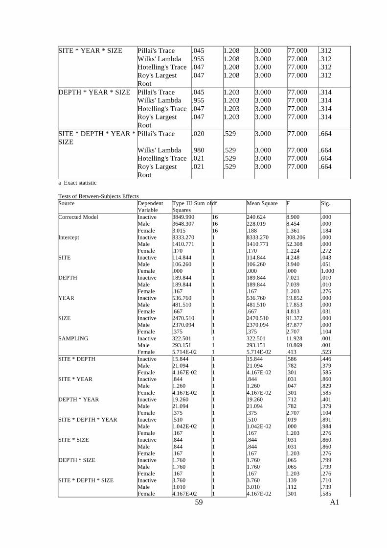
59 A1
SITE * YEAR * SIZE Pillai's Trace .045 1.208 3.000 77.000 .312 Wilks' Lambda .955 1.208 3.000 77.000 .312 Hotelling's Trace .047 1.208 3.000 77.000 .312 Roy's Largest
Root .047 1.208 3.000 77.000 .312
DEPTH * YEAR * SIZE Pillai's Trace .045 1.203 3.000 77.000 .314 Wilks' Lambda .955 1.203 3.000 77.000 .314 Hotelling's Trace .047 1.203 3.000 77.000 .314 Roy's Largest
Root .047 1.203 3.000 77.000 .314
SITE * DEPTH * YEAR * SIZE
Pillai's Trace .020 .529 3.000 77.000 .664
Wilks' Lambda .980 .529 3.000 77.000 .664 Hotelling's Trace .021 .529 3.000 77.000 .664 Roy's Largest
Root .021 .529 3.000 77.000 .664
a Exact statistic Tests of Between-Subjects Effects Source Dependent
Variable Type III Sum of Squares
df Mean Square F Sig.
Corrected Model Inactive 3849.990 16 240.624 8.900 .000 Male 3648.307 16 228.019 8.454 .000 Female 3.015 16 .188 1.361 .184 Intercept Inactive 8333.270 1 8333.270 308.206 .000 Male 1410.771 1 1410.771 52.308 .000 Female .170 1 .170 1.224 .272 SITE Inactive 114.844 1 114.844 4.248 .043 Male 106.260 1 106.260 3.940 .051 Female .000 1 .000 .000 1.000 DEPTH Inactive 189.844 1 189.844 7.021 .010 Male 189.844 1 189.844 7.039 .010 Female .167 1 .167 1.203 .276 YEAR Inactive 536.760 1 536.760 19.852 .000 Male 481.510 1 481.510 17.853 .000 Female .667 1 .667 4.813 .031 SIZE Inactive 2470.510 1 2470.510 91.372 .000 Male 2370.094 1 2370.094 87.877 .000 Female .375 1 .375 2.707 .104 SAMPLING Inactive 322.501 1 322.501 11.928 .001 Male 293.151 1 293.151 10.869 .001 Female 5.714E-02 1 5.714E-02 .413 .523 SITE * DEPTH Inactive 15.844 1 15.844 .586 .446 Male 21.094 1 21.094 .782 .379 Female 4.167E-02 1 4.167E-02 .301 .585 SITE * YEAR Inactive .844 1 .844 .031 .860 Male 1.260 1 1.260 .047 .829 Female 4.167E-02 1 4.167E-02 .301 .585 DEPTH * YEAR Inactive 19.260 1 19.260 .712 .401 Male 21.094 1 21.094 .782 .379 Female .375 1 .375 2.707 .104 SITE * DEPTH * YEAR Inactive .510 1 .510 .019 .891 Male 1.042E-02 1 1.042E-02 .000 .984 Female .167 1 .167 1.203 .276 SITE * SIZE Inactive .844 1 .844 .031 .860 Male .844 1 .844 .031 .860 Female .167 1 .167 1.203 .276 DEPTH * SIZE Inactive 1.760 1 1.760 .065 .799 Male 1.760 1 1.760 .065 .799 Female .167 1 .167 1.203 .276 SITE * DEPTH * SIZE Inactive 3.760 1 3.760 .139 .710 Male 3.010 1 3.010 .112 .739 Female 4.167E-02 1 4.167E-02 .301 .585

60 A1
YEAR * SIZE Inactive 142.594 1 142.594 5.274 .024 Male 133.010 1 133.010 4.932 .029 Female .000 1 .000 .000 1.000 SITE * YEAR * SIZE Inactive 5.510 1 5.510 .204 .653 Male 4.594 1 4.594 .170 .681 Female .375 1 .375 2.707 .104 DEPTH * YEAR * SIZE Inactive 15.844 1 15.844 .586 .446 Male 14.260 1 14.260 .529 .469 Female .375 1 .375 2.707 .104 SITE * DEPTH * YEAR * SIZE Inactive 8.760 1 8.760 .324 .571 Male 6.510 1 6.510 .241 .625 Female .000 1 .000 .000 1.000 Error Inactive 2135.999 79 27.038 Male 2130.682 79 26.971 Female 10.943 79 .139 Total Inactive 35351.000 96 Male 20357.000 96 Female 16.000 96 Corrected Total Inactive 5985.990 95 Male 5778.990 95 Female 13.958 95 a R Squared = .643 (Adjusted R Squared = .571) b R Squared = .631 (Adjusted R Squared = .557) c R Squared = .216 (Adjusted R Squared = .057) 8.3 Principal component analysis of length, height, thickness and weight total growth
(GT) Total Variance Explained Initial Eigenvalues Extraction Sums of Squared Loadings Rotation Sums of Squared
Loadings Component Total % of
Variance Cumulative %
Total % of Variance
Cumulative %
Total
1 1.834 45.841 45.841 1.834 45.841 45.841 1.802 2 1.123 28.064 73.905 1.123 28.064 73.905 1.202 3 .826 20.642 94.547 4 .218 5.453 100.000 Extraction Method: Principal Component Analysis. a When components are correlated, sums of squared loadings cannot be added to obtain a total variance. Correlation Matrix L H T W Sig. (1-tailed) L .000 .333 .213 H .000 .398 .324 T .333 .398 .289 W .213 .324 .289 Structure Matrix Component 1 2 H .937 .011 L .924 .246 T -.050 .821 W .262 .683 Extraction Method: Principal Component Analysis. Rotation Method: Oblimin with Kaiser Normalization.

61 A1
8.4 Stepwise regression analysis for the new variables LH and TW and dummy matrix
Dummy matrix
Site 1 Site 2 Depth 1 Depth 2 Year 1 Year 2 Size 1 Size 2 LH TW
1 0 1 0 1 0 1 0 0.6527 1.0689 1 0 0 1 1 0 1 0 0.5479 1.012 1 0 1 0 1 0 0 1 1.2972 0.887 1 0 0 1 1 0 0 1 0.331 0.5132 1 0 1 0 0 1 1 0 -0.3521 0.6157 1 0 0 1 0 1 1 0 -1.2958 -1.8918 1 0 1 0 0 1 0 1 0.4455 -1.8764 1 0 0 1 0 1 0 1 -0.305 -0.8596 0 1 1 0 1 0 1 0 -0.3561 1.2362 0 1 0 1 1 0 1 0 -0.348 0.0364 0 1 1 0 1 0 0 1 1.613 -0.5211 0 1 0 1 1 0 0 1 1.7057 -0.1712 0 1 1 0 0 1 1 0 -1.4591 -0.118 0 1 0 1 0 1 1 0 -1.3126 1.0737 0 1 1 0 0 1 0 1 -0.3604 -0.6803 0 1 0 1 0 1 0 1 -0.804 -0.3247 Regression for LH Model Summary Model R R Square Adjusted R Square Std. Error of the
Estimate 1 .703 .494 .458 .73642 2 .866 .750 .712 .53672 a Predictors: (Constant), Age 1 b Predictors: (Constant), Age 1, Size 1 c Dependent Variable: LH ANOVA Model Sum of
Squares df Mean Square F Sig.
1 Regression 7.408 1 7.408 13.659 .002 Residual 7.592 14 .542 Total 15.000 15 2 Regression 11.255 2 5.628 19.536 .000 Residual 3.745 13 .288 Total 15.000 15 a Predictors: (Constant), Age 1 b Predictors: (Constant), Age 1, Size 1 c Dependent Variable: LH Coefficients Unstandardized Coefficients Standardized
Coefficients t Sig.
Model B Std. Error Beta 1 (Constant) -.680 .260 -2.613 .020 Age 1 1.361 .368 .703 3.696 .002 2 (Constant) -.190 .232 -.818 .428 Age 1 1.361 .268 .703 5.071 .000 Size 1 -.981 .268 -.506 -3.655 .003

62 A1
a Dependent Variable: LH Regression for TW Model Summary Model R R Square Adjusted R Square Std. Error of the
Estimate 1 .524 .275 .223 .88141 a Predictors: (Constant), Age 1 b Dependent Variable: WT ANOVA Model Sum of
Squares df Mean Square F Sig.
1 Regression 4.124 1 4.124 5.308 .037 Residual 10.876 14 .777 Total 15.000 15 a Predictors: (Constant), Age 1 b Dependent Variable: WT Coefficients Unstandardized Coefficients
Standardized Coefficients
t Sig.
Model B Std. Error Beta 1 (Constant) -.508 .312 -1.629 .126 Age 1 1.015 .441 .524 2.304 .037 a Dependent Variable: WT 8.5 Principal component analysis of monthly instantaneous growth rate (G30) of shell
length, height, thickness and wet weight Total Variance Explained Initial Eigenvalues
Extraction Sums of Squared Loadings
Component Total % of Variance Cumulative %
Total % of Variance Cumulative %
1 3.145 78.635 78.635 3.145 78.635 78.635 2 .582 14.542 93.176 3 .176 4.406 97.582 4 9.673E-02 2.418 100.000 Extraction Method: Principal Component Analysis. Correlation Matrixa
L MIG H MIG T MIG W MIG Correlation L MIG 1.000 .893 .522 .863 H MIG .893 1.000 .578 .828 T MIG .522 .578 1.000 .548 W MIG .863 .828 .548 1.000 Sig. (1-tailed) L MIG .000 .000 .000 H MIG .000 .000 .000 T MIG .000 .000 .000 W MIG .000 .000 .000 Determinant = 3.119E-02 Rotated Component Matrix a Only one component was extracted. The solution cannot be rotated. Component Matrix Component

63 A1
1 H MIG .942 L MIG .939 W MIG .925 T MIG .723 Extraction Method: Principal Component Analysis. a 1 components extracted. Communalities Initial Extraction L MIG 1.000 .882 H MIG 1.000 .887 T MIG 1.000 .522 W MIG 1.000 .856 Extraction Method: Principal Component Analysis. 8.6 Univariate ANOVA to test if sampling, site, depth, age and size has an effect on
G30 factor scores Tests of Between-Subjects Effects Dependent Variable: G30 factor
Source Type III Sum of Squares
df Mean Square F Sig.
Corrected Model 78.455 75 1.046 7.684 .029 Intercept .000 1 .000 .000 1.000 YEAR 10.744 1 10.744 78.924 .001 SIZE 6.498 1 6.498 47.732 .002 SITE 4.302E-02 1 4.302E-02 .316 .604 DEPTH 1.765E-02 1 1.765E-02 .130 .737 SAMPLING 29.841 4 7.460 54.803 .001 YEAR * SIZE .693 1 .693 5.094 .087 YEAR * SITE 8.532E-03 1 8.532E-03 .063 .815 SIZE * SITE .273 1 .273 2.003 .230 YEAR * SIZE * SITE 6.992E-02 1 6.992E-02 .514 .513 YEAR * DEPTH 1.313E-02 1 1.313E-02 .096 .772 SIZE * DEPTH 9.516E-02 1 9.516E-02 .699 .450 YEAR * SIZE * DEPTH 1.071E-02 1 1.071E-02 .079 .793 SITE * DEPTH 9.500E-03 1 9.500E-03 .070 .805 YEAR * SITE * DEPTH 1.745E-03 1 1.745E-03 .013 .915 SIZE * SITE * DEPTH 3.219E-03 1 3.219E-03 .024 .885 YEAR * SIZE * SITE * DEPTH .390 1 .390 2.866 .166 YEAR * SAMPLING 15.144 4 3.786 27.811 .004 SIZE * SAMPLING 1.799 4 .450 3.304 .137 YEAR * SIZE * SAMPLING .804 4 .201 1.476 .358 SITE * SAMPLING 1.511 4 .378 2.774 .173 YEAR * SITE * SAMPLING 1.645 4 .411 3.021 .155 SIZE * SITE * SAMPLING 1.315 4 .329 2.415 .207 YEAR * SIZE * SITE * SAMPLING 2.221 4 .555 4.079 .101 DEPTH * SAMPLING 1.518 4 .379 2.788 .172 YEAR * DEPTH * SAMPLING .555 4 .139 1.019 .493 SIZE * DEPTH * SAMPLING 1.005 4 .251 1.846 .284 YEAR * SIZE * DEPTH * SAMPLING 1.034 4 .259 1.899 .275 SITE * DEPTH * SAMPLING .527 4 .132 .968 .512 YEAR * SITE * DEPTH * SAMPLING 1.742E-02 4 4.355E-03 .032 .997 SIZE * SITE * DEPTH * SAMPLING .649 4 .162 1.191 .435 Error .545 4 .136 Total 79.000 80 Corrected Total 79.000 79

64 A1
a R Squared = .993 (Adjusted R Squared = .864)
Multiple Comparisons Dependent Variable: G30 factor Bonferroni (I) Sampling (J) Sampling Mean Difference
(I-J)
Std. Error
Sig.
95% Confidence Interval Lower Bound Upper Bound
Aug Sep -1.7045887 .13044596 .002 -2.4347688 -.9744085 Oct -.1666138 .13044596 1.000 -.8967940 .5635663 Nov -.4364495 .13044596 .287 -1.1666296 .2937307 Dec -.2758143 .13044596 1.000 -1.0059945 .4543659 Sep Aug 1.7045887 .13044596 .002 .9744085 2.4347688 Nov 1.5379748 .13044596 .003 .8077947 2.2681550 Dec 1.2681392 .13044596 .006 .5379590 1.9983193 Jan 1.4287744 .13044596 .004 .6985942 2.1589545 Nov Aug .1666138 .13044596 1.000 -.5635663 .8967940 Sep -1.5379748 .13044596 .003 -2.2681550 -.8077947 Dec -.2698356 .13044596 1.000 -1.0000158 .4603445 Jan -.1092005 .13044596 1.000 -.8393806 .6209797 Dec Aug .4364495 .13044596 .287 -.2937307 1.1666296 Sep -1.2681392 .13044596 .006 -1.9983193 -.5379590 Nov .2698356 .13044596 1.000 -.4603445 1.0000158 Jan .1606352 .13044596 1.000 -.5695450 .8908153 Jan Aug .2758143 .13044596 1.000 -.4543659 1.0059945 Sep -1.4287744 .13044596 .004 -2.1589545 -.6985942 Nov .1092005 .13044596 1.000 -.6209797 .8393806 Dec -.1606352 .13044596 1.000 -.8908153 .5695450 Based on observed means. * The mean difference is significant at the .05 level. 8.7 Multiple linear regression analysis of log10 condition index and environmental
variables Correlations
LOGCI SPM POM pH Salinity Temperature Rainfall chloroa chlorob chloroc Pearson
Correlation LOGCI 1.000 .097 .086 .058 .243 .204 -.005 .099 .128 .115
SPM .097 1.000 .405 -.553 -.242 -.322 -.198 .501 .526 .533 POM .086 .405 1.000 -.519 -.335 -.540 -.458 .569 .570 .586 pH .058 -.553 -.519 1.000 .570 .526 .091 -.619 -.588 -.627 Salinity .243 -.242 -.335 .570 1.000 .446 .258 -.302 -.280 -.310 Temperature .204 -.322 -.540 .526 .446 1.000 .618 -.218 -.191 -.223 Rainfall -.005 -.198 -.458 .091 .258 .618 1.000 -.224 -.250 -.238 chloroa .099 .501 .569 -.619 -.302 -.218 -.224 1.000 .988 .994 chlorob .128 .526 .570 -.588 -.280 -.191 -.250 .988 1.000 .996 chloroc .115 .533 .586 -.627 -.310 -.223 -.238 .994 .996 1.000
Sig. (1-tailed)
LOGCI . .174 .202 .288 .008 .023 .480 .168 .107 .131
SPM .174 . .000 .000 .009 .001 .027 .000 .000 .000 POM .202 .000 . .000 .000 .000 .000 .000 .000 .000 pH .288 .000 .000 . .000 .000 .189 .000 .000 .000 Salinity .008 .009 .000 .000 . .000 .006 .001 .003 .001 Temperature .023 .001 .000 .000 .000 . .000 .016 .032 .014 Rainfall .480 .027 .000 .189 .006 .000 . .014 .007 .010 chloroa .168 .000 .000 .000 .001 .016 .014 . .000 .000 chlorob .107 .000 .000 .000 .003 .032 .007 .000 . .000 chloroc .131 .000 .000 .000 .001 .014 .010 .000 .000 .

65 A1
Model Summary Model R R Square Adjusted R
Square Std. Error
of the Estimate
Change Statistics R Square Change
F Change df1 df2 Sig. F Change
1 .433 .188 .103 .13561 .188 2.210 9 86 .029 a Predictors: (Constant), chloroc, Temperature, Salinity, SPM, Rainfall, POM, pH, chloroa, chlorob ANOVA
Model Sum of Squares df Mean Square F Sig. 1 Regression .366 9 .041 2.210 .029
Residual 1.581 86 .018 Total 1.947 95
a Predictors: (Constant), chloroc, Temperature, Salinity, SPM, Rainfall, POM, pH, chloroa, chlorob b Dependent Variable: LOGCI Coefficients Unstandardized
Coefficients
Standardized Coefficients
t Sig. Correlations
Model B Std. Error Beta Zero-order Partial Part 1 (Constant) -3.749 1.608 -2.332 .022 SPM 2.887 5.794 .065 .498 .620 .097 .054 .048 POM 7.607 6.311 .175 1.205 .231 .086 .129 .117 pH -.126 .150 -.169 -.839 .404 .058 -.090 -.082 Salinity 8.432E-02 .035 .304 2.417 .018 .243 .252 .235 Temperature .136 .056 .457 2.421 .018 .204 .253 .235 Rainfall -3.445E-04 .000 -.251 -1.519 .132 -.005 -.162 -.148 chloroa -.550 .542 -1.037 -1.015 .313 .099 -.109 -.099 chlorob -.281 .513 -.732 -.548 .585 .128 -.059 -.053 chloroc .239 .252 1.769 .947 .346 .115 .102 .092 a Dependent Variable: LOGCI 8.8 Principal component analysis of environmental parameters Total Variance Explained
Initial Eigenvalues Extraction Sums of Squared Loadings
Rotation Sums of Squared Loadings
Component Total % of Variance
Cumulative %
Total % of Variance
Cumulative %
Total % of Variance
Cumulative %
1 4.823 53.584 53.584 4.823 53.584 53.584 3.986 44.290 44.290 2 1.595 17.724 71.308 1.595 17.724 71.308 2.432 27.017 71.308 3 .960 10.664 81.972 4 .669 7.433 89.405 5 .474 5.265 94.670 6 .342 3.804 98.474 7 .127 1.408 99.883 8 8.767E-03 9.741E-02 99.980 9 1.802E-03 2.002E-02 100.000
Extraction Method: Principal Component Analysis Correlation Matrix SPM POM pH Salinity Temperature Rainfall Chloro a Chloro b Chloro c Correlation SPM 1.000 .405 -.553 -.242 -.322 -.198 .501 .526 .533 POM .405 1.000 -.519 -.335 -.540 -.458 .569 .570 .586 pH -.553 -.519 1.000 .570 .526 .091 -.619 -.588 -.627 Salinity -.242 -.335 .570 1.000 .446 .258 -.302 -.280 -.310
Temperature -.322 -.540 .526 .446 1.000 .618 -.218 -.191 -.223
Rainfall -.198 -.458 .091 .258 .618 1.000 -.224 -.250 -.238 chloroa .501 .569 -.619 -.302 -.218 -.224 1.000 .988 .994

66 A1
chlorob .526 .570 -.588 -.280 -.191 -.250 .988 1.000 .996 chloroc .533 .586 -.627 -.310 -.223 -.238 .994 .996 1.000 Sig. (1-tailed) SPM .025 .003 .127 .063 .177 .006 .004 .004 POM .025 .005 .055 .003 .012 .002 .002 .001 pH .003 .005 .002 .004 .336 .001 .001 .001
Salinity .127 .055 .002 .014 .112 .075 .093 .070 Temperature
.063 .003 .004 .014 .001 .153 .186 .147
Rainfall .177 .012 .336 .112 .001 .147 .119 .131 chloroa .006 .002 .001 .075 .153 .147 .000 .000 chlorob .004 .002 .001 .093 .186 .119 .000 .000 chloroc .004 .001 .001 .070 .147 .131 .000 .000
a Determinant = 1.604E-06 Rotated Component Matrix
Component
1 2 chloroc .973 -.132 chlorob .968 -.107 chloroa .967 -.118 pH -.659 .445 SPM .604 -.282 Temperature -.101 .914 Rainfall -5.745E-02 .759 Salinity -.260 .600 POM .537 -.582 Extraction Method: Principal Component Analysis. Rotation Method: Varimax with Kaiser Normalization. a Rotation converged in 3 iterations 8.9 Multivariate analysis of covariance of component 1 (Food), component 2
(Physical) scores and pH Levene's Test of Equality of Error Variances
F df1 df2 Sig. Food .635 3 20 .601 physical .460 3 20 .713 PH .769 3 20 .525 Tests the null hypothesis that the error variance of the dependent variable is equal across groups.a Design: Intercept+TIME+SITE+DEPTH+SITE * DEPTH Multivariate Tests
Effect Value F Hypothesis df Error df Sig. Intercept Pillai's Trace .999 9162.612 3.000 17.000 .000 Wilks' Lambda .001 9162.612 3.000 17.000 .000 Hotelling's Trace 1616.932 9162.612 3.000 17.000 .000 Roy's Largest Root 1616.932 9162.612 3.000 17.000 .000 TIME Pillai's Trace .909 56.778 3.000 17.000 .000 Wilks' Lambda .091 56.778 3.000 17.000 .000 Hotelling's Trace 10.020 56.778 3.000 17.000 .000 Roy's Largest Root 10.020 56.778 3.000 17.000 .000 SITE Pillai's Trace .183 1.272 3.000 17.000 .316 Wilks' Lambda .817 1.272 3.000 17.000 .316 Hotelling's Trace .224 1.272 3.000 17.000 .316 Roy's Largest Root .224 1.272 3.000 17.000 .316 DEPTH Pillai's Trace .188 1.316 3.000 17.000 .302 Wilks' Lambda .812 1.316 3.000 17.000 .302 Hotelling's Trace .232 1.316 3.000 17.000 .302 Roy's Largest Root .232 1.316 3.000 17.000 .302 SITE * DEPTH Pillai's Trace .223 1.622 3.000 17.000 .221

67 A1
Wilks' Lambda .777 1.622 3.000 17.000 .221 Hotelling's Trace .286 1.622 3.000 17.000 .221 Roy's Largest Root .286 1.622 3.000 17.000 .221 a Exact statistic b Design: Intercept+TIME+SITE+DEPTH+SITE * DEPTH Tests of Between-Subjects Effects Source Dependent
Variable Type III Sum
of Squares df Mean Square F Sig.
Corrected Model food 15.077 4 3.769 9.039 .000 physical 7.964 4 1.991 2.516 .076 pH .717 4 .179 21.529 .000 Intercept food 10.788 1 10.788 25.870 .000 physical 4.096 1 4.096 5.176 .035 pH 254.278 1 254.278 30543.181 .000 TIME food 13.356 1 13.356 32.030 .000 physical 5.072 1 5.072 6.409 .020 pH .670 1 .670 80.517 .000 SITE food 1.293 1 1.293 3.101 .094 physical 1.501 1 1.501 1.896 .184 pH 8.067E-03 1 8.067E-03 .969 .337 DEPTH food .421 1 .421 1.009 .328 physical 1.625E-03 1 1.625E-03 .002 .964 pH 1.927E-02 1 1.927E-02 2.314 .145 SITE * DEPTH food 7.811E-03 1 7.811E-03 .019 .893 physical 1.390 1 1.390 1.757 .201 pH 1.927E-02 1 1.927E-02 2.314 .145 Error food 7.923 19 .417 physical 15.036 19 .791 pH .158 19 8.325E-03 Total food 23.000 24 physical 23.000 24 pH 1447.961 24 Corrected Total food 23.000 23 physical 23.000 23 pH .875 23 a R Squared = .656 (Adjusted R Squared = .583),b R Squared = .346 (Adjusted R Squared = .209),c R Squared = .819 (Adjusted R Squared = .781) 8.10 Discriminant analysis of sex, size (length, height, thickness) and weight Eigenvalues Function Eigenvalue % of Variance Cumulative % Canonical
Correlation 1 .241 99.4 99.4 .441 2 .002 .6 100.0 .039 a First 2 canonical discriminant functions were used in the analysis. Wilks' Lambda Test of Function(s) Wilks' Lambda Chi-square df Sig. 1 through 2 .804 625.178 6 .000 2 .998 4.484 2 .106 Standardized Canonical Discriminant Function Coefficients Function 1 2 LENGTH .255 1.884

68 A1
HEIGHT .315 -.083 WEIGHT .479 -1.736 Structure Matrix Function 1 2 WEIGHT .967 -.210 HEIGHT .948 .045 LENGTH .933 .339 THICKNESSa .714 -.084 a This variable not used in the analysis. Functions at Group Centroids Function SEX 1 2 .00 -.414 -1.284E-03 1.00 .578 8.458E-03 2.00 .850 -.561 Unstandardized canonical discriminant functions evaluated at group means Classification Function Coefficients SEX .00 1.00 2.00 LENGTH .523 .537 .484 HEIGHT .771 .788 .796 WEIGHT -.169 -.165 -.154 (Constant) -59.130 -64.693 -66.408 Fisher's linear discriminant functions Classification Results Predicted Group Membership
Total
SEX .00 1.00 2.00 Original Count .00 1349 330 0 1679 1.00 505 678 0 1183 2.00 5 9 0 14 % .00 80.3 19.7 .0 100.0 1.00 42.7 57.3 .0 100.0 2.00 35.7 64.3 .0 100.0 a 70.5% of original grouped cases correctly classified. 8.11 Pearson’s correlation between inactive, male and female oysters and
environmental parameters Correlations Inacti
ve Male Fema
le SPM POM pH Salini
ty Temperature
Rainfall
Chloro a
Chloro b
Chloro c
Inactive Pearson 1 -.998 -.359 .114 .053 -.209 -.062 -.261 -.217 .073 .083 .090

69 A1
Correlation Sig. (2-tailed) . .000 .000 .268 .606 .041 .545 .010 .034 .481 .421 .386 N 96 96 96 96 96 96 96 96 96 96 96 96 Male Pearson
Correlation -.998 1 .319 -.113 -.048 .204 .055 .261 .217 -.071 -.081 -.087
Sig. (2-tailed) .000 . .002 .271 .642 .046 .594 .010 .034 .494 .432 .397 N 96 96 96 96 96 96 96 96 96 96 96 96 Female Pearson
Correlation -.359 .319 1 .084 -.029 .052 .091 .070 .164 .050 .051 .042
Sig. (2-tailed) .000 .002 . .418 .780 .613 .380 .499 .110 .629 .625 .687 N 96 96 96 96 96 96 96 96 96 96 96 96 SPM Pearson
Correlation .114 -.113 .084 1 .405 -.553 -.242 -.322 -.198 .501 .526 .533
Sig. (2-tailed) .268 .271 .418 . .000 .000 .017 .001 .053 .000 .000 .000 N 96 96 96 96 96 96 96 96 96 96 96 96 POM Pearson
Correlation .053 -.048 -.029 .405 1 -.519 -.335 -.540 -.458 .569 .570 .586
Sig. (2-tailed) .606 .642 .780 .000 . .000 .001 .000 .000 .000 .000 .000 N 96 96 96 96 96 96 96 96 96 96 96 96 pH Pearson
Correlation -.209 .204 .052 -.553 -.519 1 .570 .526 .091 -.619 -.588 -.627
Sig. (2-tailed) .041 .046 .613 .000 .000 . .000 .000 .377 .000 .000 .000 N 96 96 96 96 96 96 96 96 96 96 96 96 Salinity Pearson
Correlation -.062 .055 .091 -.242 -.335 .570 1 .446 .258 -.302 -.280 -.310
Sig. (2-tailed) .545 .594 .380 .017 .001 .000 . .000 .011 .003 .006 .002 N 96 96 96 96 96 96 96 96 96 96 96 96 Temperature
Pearson Correlation
-.261 .261 .070 -.322 -.540 .526 .446 1 .618 -.218 -.191 -.223
Sig. (2-tailed) .010 .010 .499 .001 .000 .000 .000 . .000 .033 .063 .029 N 96 96 96 96 96 96 96 96 96 96 96 96 Rainfall Pearson
Correlation -.217 .217 .164 -.198 -.458 .091 .258 .618 1 -.224 -.250 -.238
Sig. (2-tailed) .034 .034 .110 .053 .000 .377 .011 .000 . .028 .014 .019 N 96 96 96 96 96 96 96 96 96 96 96 96 Chloroa Pearson
Correlation .073 -.071 .050 .501 .569 -.619 -.302 -.218 -.224 1 .988 .994
Sig. (2-tailed) .481 .494 .629 .000 .000 .000 .003 .033 .028 . .000 .000 N 96 96 96 96 96 96 96 96 96 96 96 96 Chlorob Pearson
Correlation .083 -.081 .051 .526 .570 -.588 -.280 -.191 -.250 .988 1 .996
Sig. (2-tailed) .421 .432 .625 .000 .000 .000 .006 .063 .014 .000 . .000 N 96 96 96 96 96 96 96 96 96 96 96 96 Chloroc Pearson
Correlation .090 -.087 .042 .533 .586 -.627 -.310 -.223 -.238 .994 .996 1
Sig. (2-tailed) .386 .397 .687 .000 .000 .000 .002 .029 .019 .000 .000 . N 96 96 96 96 96 96 96 96 96 96 96 96 ** Correlation is significant at the 0.01 level (2-tailed). Correlation is significant at the 0.05 level (2-tailed).

286
APPENDIX B
CHEMICALS AND FIXATIVES
Chapter 3
90 % Acetone (v/v) Acetone 90 ml Add to 10 ml distilled water
Chapter 8 FAACC gonad fixative 40% Formaldehyde solution 10 ml Glacial acetic acid 5 ml Calcium chloride dihydrate 1.3 g Add to 85 ml of distilled water.

Appendix C – Histology
287
APPENDIX C
HISTOLOGY
Figure 1 Photo and micrograph of Stage 1 female P. maxima.
(a) Sex can be determined as female based on colour (yellowish-
orange) but development is slight and patchy. The gonad (G) is still flaccid and the colour somewhat dull and development is only along the base of the digestive diverticulum (DD).
(b) Early oogenesis. Acinus show some stem cells (sc), oogonia (og)
and young oocytes (y oc) developing along the inner wall. Larger and older oocytes (o oc) are found further within the acinar lumen. Interconnective tissue (ict) support area between acini.
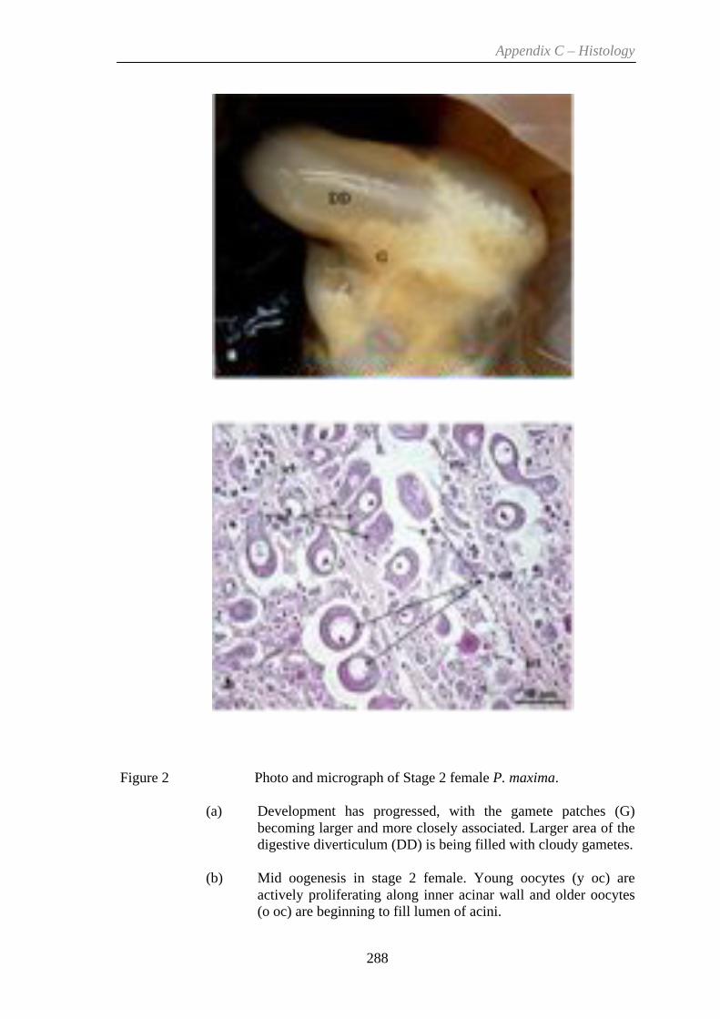
Appendix C – Histology
288
Figure 2 Photo and micrograph of Stage 2 female P. maxima.
(a) Development has progressed, with the gamete patches (G) becoming larger and more closely associated. Larger area of the digestive diverticulum (DD) is being filled with cloudy gametes.
(b) Mid oogenesis in stage 2 female. Young oocytes (y oc) are
actively proliferating along inner acinar wall and older oocytes (o oc) are beginning to fill lumen of acini.

Appendix C – Histology
289
Figure 3 Photo and micrograph of Stage 3 female P. maxima.
(a) Patches of gametes are more confluent and have taken on a more solid appearance. Gametes (G) are visible along length of digestive diverticulum.
(b) Mid-developmental phase of stage 3 female. Acini are still
visible and lumens of acini are filled with increasingly larger free oocytes (f oc) and acinar-connected oocytes (c oc). The proportion of interconnective tissue (ict) between acini is decreasing.

Appendix C – Histology
290
Figure 4 Photo and micrograph of Stage 4 female P. maxima.
(a) Gonad (G) is turgid, however, only one side of the gonad is well developed.
(b) Actively developing ovary. Acini start to become confluent (conf)
and are filled with free oocytes (f oc) and connected oocytes (c oc).

Appendix C – Histology
291
Figure 5 Photo and micrograph of Stage 5 female P. maxima.
(a) Female gonads (G) now appear as bands of colour with both sides of the gonad well developed and visible along the length of the digestive diverticulum (DD).
(b) Near ripe ovary. More acini become confluent and lumen starts to
be filled with greater number of free oocytes, although connected oocytes are still observed.

Appendix C – Histology
292
Figure 6 Photo and micrograph of Stage 1 male P. maxima.
(a) Male gonad (G) is clearly visible as creamy white patches. Patches are visible at the base of the digestive diverticulum (DD) around the dorsal edge of the retractor muscle (RM).
(b) Early stages of gametogenesis. Large spermatogonia (sg) lining inner wall of acinus and sparse spermatocytes (sc) and greater number of spermatids (st) visible in the inner lumen. Tails of spermatozoa (sz) can be seen within the pockets of spermatids.

Appendix C – Histology
293
Figure 7 Photo and micrograph of Stage 2 male P. maxima.
(a) Gametes (G) have moved further along the base of the digestive
diverticulum (DD). Development is still patchy and cloudy. (b) Actively developing testis. Spermatogonia (sg) can be seen
lining the inner wall of acini, large spermatocytes (sc) and small spermatids (st) are scattered at the periphery while spermatozoa (sz) with visible tails are in the centre.

Appendix C – Histology
294
Figure 8 Photo and micrograph of Stage 3 male P. maxima.
(a) Gametes (G) patches have become larger and progressed further along the digestive diverticulum (DD). Development is observed on only one side of the digestive diverticulum.
(b) Near ripe testis. Within the acinus, the outer darker bands of cells at the border are developing sperm (ds) while the more mature spermatozoa (sz) fill the middle with tails visible.

Appendix C – Histology
295
Figure 9 Photo and micrograph of Stage 4 male P. maxima.
(a) Gonad is turgid. Patches are large and more confluent and only one side of the digestive diverticulum has well developed gametes.
(b) Near ripe testis, with confluent acini filled predominantly with
sperm in the later stages of development i.e spermatids (st) and spermatozoa with tails (sz). Small bands of spermatocytes (sc) can also be seen.

Appendix C – Histology
296
Figure 10 Photo and micrograph of Stage 5 male P. maxima.
(a) Gonad patches are found along both sides of the digestive diverticulum and are well developed.
(b) Near ripe testis. Acini are packed tightly with sperm cells, with
spermatozoa (sz) in the centre of each lumen. Interconnective tissue (ict) between acini start to decrease.
sz
ict
sz
sz
ict
sz

Appendix C – Histology
297
Figure 11 Photo and micrograph of Stage 6 male P. maxima.
(a) The digestive diverticulum is turgid and filled with gametes. Gonad is full.
(b) Boundaries between acini are difficult to distinguish. Acini are fully
filled with mature sperm cells.
G
DD
G
a

298
APPENDIX D
Publication

CSIRO PUBLISHING
Marine and Freshwater Research, 2008, 59, 22–31 www.publish.csiro.au/journals/mfr
Modelling and comparison of growth of the silver-lip pearloyster Pinctada maxima (Jameson) (Mollusca : Pteriidae)cultured in West Papua, Indonesia
Anne M. LeeA,C, Ashley J. WilliamsB and Paul C. SouthgateA
APearl Oyster Research Group, School of Marine and Tropical Biology,James Cook University, Qld 4811, Australia.
BFishing and Fisheries Research Centre, School of Earth and Environmental Science,James Cook University, Qld 4811, Australia.
CCorresponding author. Email: [email protected]
© CSIRO 2008 10.1071/MF07112 1323-1650/08/010022

Growth of P. maxima cultured in West Papua Marine and Freshwater Research 23

24 Marine and Freshwater Research A. M. Lee et al.

Growth of P. maxima cultured in West Papua Marine and Freshwater Research 25

26 Marine and Freshwater Research A. M. Lee et al.

Growth of P. maxima cultured in West Papua Marine and Freshwater Research 27

28 Marine and Freshwater Research A. M. Lee et al.

Growth of P. maxima cultured in West Papua Marine and Freshwater Research 29

30 Marine and Freshwater Research A. M. Lee et al.

Growth of P. maxima cultured in West Papua Marine and Freshwater Research 31
http://www.publish.csiro.au/journals/mfr