1

Spatial Variability of Soil Organic Carbon in a Cassava field at Ekha Agro Farms, Lanlate, Oyo State, Nigeria

1Alabi , R.T., and 2Jayeoba O. J

1. Geospatial Laboratory, International Institute of Tropical Agriculture, Ibadan. Nigeria 2. Agronomy Department, Faculty of Agriculture, Nasarawa State University, Keffi, Lafia Campus, Nigeria

Abstract

Soil Organic Carbon (SOC) is one of the most important parameters affecting the chemical, physical and hydraulic characteristics of natural soils. Knowledge of spatial variability in soil fertility is important for site specific nutrient management. The study was conducted on a 467 hectare commercial cassava farm located at Lanlate (7º 36'N and 3º 27'E), Oyo State, southwestern Nigeria. Soil samples were collected from eighty–eight (88) sites on a grid system at 0-30 cm and 30-60 cm depths. Coordinates (latitude and longitude) of the locations of the sampling sites were obtained with the aid of a hand held Global Positioning System (GPS) (Garmin eTrex Ventura®) receiver,. The Walkley and Black (1934) wet digestion method was used to determine soil organic carbon content. Spatial analysis of the classified SOC was done in a GIS environment. A GIS software package ArcGIS 10.2 and ArcGIS Geo-statistical Analyst Extension were used. Various interpolation techniques, ordinary kriging, Simple Normal Score, Universal kriging, Empirical Bayesian Kriging and Ordinary co-kriging were used to produce the spatial distribution of the SOC. Ordinary co-Kriging with Nitrogen as a covariate gave the best model predictions for both surface and sub-surface depth. The best fit semivariogram models for SOC were “K-Bessel” and “J-Bessel” for surface and subsurface depths respectively. The nugget-to-sill ratio(Co/Co + C) for soil organic carbon at the surface depth was 0.103 and 0.062 for sub surface soil, these indicated a strong spatial dependence for both top soil and subsoil. The spatial distribution of soil organic carbon at Ekha farm is dominated by the constitutive factors and the random factors together. Based on the spatial interpolation, two management zones were delineated for SOC at the surface depth. Keywords: Precision Farming, Soil Organic Carbon, Semi -variogram, Spatial pattern, Kriging and Modeling.

Introduction

Soil organic carbon (SOC) is a complex and varied mixture of materials and makes up a small but vital part of all soils (CSIRO, 2011). Soil carbon improves the physical properties of soil. It increases the cation exchange capacity (CEC) and water-holding capacity of sandy soil and it contributes to the structural stability of clay soils by helping to bind particles into aggregates. (Leeper and Uren,1993). Soil organic matter, of which carbon is a major part, holds a great proportion of nutrients, cations and trace elements that are of importance to plant growth. It prevents nutrient leaching and is integral to the organic acids that make minerals available to plants. It also buffers soil from strong changes in pH (Leu, 2007). It is widely accepted that the carbon content of soil is a major factor in its overall health. SOC is the largest carbon (C) reservoir in many terrestrial ecosystems including grasslands, savannas, boreal forests, tundra, some temperate forests, and cultivated systems, comprising as much as 98% of ecosystem C stocks in some systems (Schlesinger, 1977). Globally, the amount of C stored in soil is equal to

2

the amount stored in vegetation and in the atmosphere combined (Schimel, 1995). Natural variations in SOC occur as a result of climate, organisms, parent material, time and relief (Young and Young, 2001). The greatest contemporary influence has been that of humans (CSIRO, 2011). The traditional approach to soil fertility management has been to treat fields as homogenous areas and to calculate fertilizer requirements on a whole field basis. However, it has been reported for at least 70 years that fields are not homogeneous and sampling techniques to describe field variability have been recommended (Flower et al., 2005, Santra et al., 2008). Describing the spatial variability across a field has been difficult until new technologies such as Global Positioning Systems (GPS) and Geographic Information Systems (GIS) were introduced. GIS is a powerful set of tools for collecting, storing, retrieving, transforming and displaying spatial data (Burrough, and McDonnell, 1998). GIS can be used in producing soil fertility map of an area that helps to understand the status of soil fertility spatially and temporally, which will help in formulating site-specific balanced fertilizer recommendation. These technologies allow fields to be mapped accurately and also allow complex spatial relationships between soil fertility factors to be computed (Patil et al., 2011) Geostatistics (e.g., Goovaerts, 1997; Webster and Oliver, 2001; Nielsen and Wendroth, 2003) has been extensively used for quantifying the spatial pattern of environmental variables. Kriging has been used for many decades as synonym for geostatistical interpolation and has been proved as sufficiently robust for estimating values at unsampled locations based on the sampled data. In recent years soil scientists focused on using geostatistics and different kriging methods to predict soil properties at unsampled locations and to better understand their spatial variability pattern over small large spatial scale. (Yost et al., 1982; Trangmar et al., 1987; Miller et al., 1988; Voltz and Webster, 1990; Chien et al., 1997; Lark, 2002). The purpose of this present study was, thus, to investigate the spatial variability of the soil organic carbon at two different soil layers in a cassava field. MATERIALS AND METHODS Description of the study area The study was conducted on a 467 hectare commercial cassava farm located at Lanlate (7º 36'N and 3º 27'E), Oyo State, southwestern Nigeria (Fig 1). The climate of lanlate area is hot subhumid and lies within the derived savanna zone, with annual rainfall of between 1200 and 1500 mm. The relative humidity is over 70% in the morning and falls to between 50 and 70% in the afternoon. The mean annual temperature is 27°C and the annual temperature range is 8°C. Some of the dominant vegetal species include Panicum maximum, Imperata cylindrical, Andropogon gayanus, Chromolaena odorata, Eupatorium odoratum, Tithonia diversifofolia, Parkia biglobosa, Vitellaria paradoxa, and Piliostigma reticulatal. The soils in the study area are Ferric Luvisols (Sonelveld, 2005). The study area was planted to cassava at different stages of growth (Figure 2). Soil samples were collected from eighty–eight (88) sites on a grid system using Global Positioning System (GPS), at 0-30 cm and 30-60 cm depths. The samples were air dried, crushed and passed through 2 mm sieve prior to analysis. The Walkley and Black (1934) wet digestion method was used to determine soil organic carbon content.

3

Figure 1: Map of the study area showing soil sampling locations (n=88)

Figure 2: View of the study area planted to cassava at different stages of growth.

4

Statistical analysis Exploratory data analysis was performed by SPSS (version 16) software. The data distributions were analyzed by classical statistics (mean maximum, minimum, standard deviation, skewness, kurtosis and coefficient of variation). Histograms and Box-plots for organic carbon data were inspected for the possible outliers which affect the descriptive statistics and the characterization of spatial variation. Geostatistical methods require using data with normal distribution values, SOC data was also checked for normality and transformed as appropriate. Spatial analysis of the classified soil organic carbon was performed in a GIS environment. Experimental semi-variograms were calculated for the two depths using equation (1)

…………………….. (1)

Where γ(h) is the semivariance for the lag distance h. N (h) is the number of sample pairs separated by the lag distance h, z(xα) is the measured value at αth sample location and z(xα+h) is the measured value at point α+hth sample location. Theoretical models (Spherical, Rational Quadratic, Hole effect, Exponential, K-Bessel or Gaussian) were fitted to experimental semivariograms. A GIS software package ArcGIS 10.1 and ArcGIS Geo-statistical Analyst Extension were used. Model selection for semivariograms was done on the basis of goodness of model fit criterion. Various interpolation techniques, ordinary Kriging, Simple Normal Score, Universal Kriging, Empirical Bayesian Kriging and Ordinary co-Kriging were used to produce the spatial distribution of the SOC. The possible effect of covariates on the prediction of SOC was explored. Hence Cokriging was performed with Nitrogen, Calcium, Phosphorus, CEC, Magnesium, Potassium, Iron, Sodium, elevation, Enhanced Vegetation Index (EVI) and Normalized Difference Vegetation Index (NDVI) as covariates with SOC. Long term average EVI and NDVI were obtained from AfSIS (2014).

Table 1 Organic Carbon Rating and Interpretations

Range (%) Class < 0.4 Very low

0.4 – 1.0 Low 1.0 – 1.5 Moderate 1.5 – 2.0 High

>2.0 Very high RESULTS AND DISCUSSION Statistical parameters of soil organic carbon The summary statistical parameters of the soil organic carbon data set were listed in Table 2. To evaluate the data set, the mean, minimum values, maximum values, median values, standard

5

deviation and variance were calculated. The organic carbon at the surface (0-30cm) depth ranged from 0.53 to 2.15 (mean = 1.0405), while that of the sub surface (30-60cm) soil ranged from 0.33 to 2.13. Kriging methods work best if the data is approximately normally distributed. In ArcGIS Geostatistical Analyst, the histogram and normal QQPlots were used to see what transformations, if any, are needed to make the data more normally distributed. Normal QQPlots provides an indication of univariate normality. Histogram and normal QQPlots analysis were applied for each soil organic carbon parameter and the results are presented in Figure 3. It was found that all the parameters required transformation for it to conform to the normality requirement of Kriging. For these parameters a log transformations were applied to make the distribution close to normal Table 2. Summary Statistical parameters of soil organic carbon at surface (0-30) and sub surface (30-60) depths

Soil Organic Carbon

30cm 60cm N 88 87 Mean 1.0405 0.7157 Std. Deviation 0.33469 0.30830 Variance 0.112 0.095 Skewness 1.268 1.834 Std. Error of Skewness 0.257 0.258 Kurtosis 1.903 4.935 Std. Error of Kurtosis 0.508 0.511 Range 1.63 1.80 Minimum 0.53 0.33 Maximum 2.16 2.13

Semivariogram models The prediction of the spatial process at nonsampling sites using geostatistics requires a theoretical semivariogram. It is necessary to decide on a theoretical variogram based on the experimental variogram. It is vital to choose an appropriate model to estimate spatial statistics as each model yields different values for nugget variance and range which are essential for geostatistical analyses (Trangmar, 1985). In this study, the semivariogram models (Circular, Spherical, Tetraspherical, Pentaspherical, Exponential, Gaussian, Rational Quadratic, Hole effect, K-Bessel, J-Bessel, Stable) were tested with optimized parameters. Prediction performances were assessed by cross validation. Cross Validation allows determination of which model provides the best predictions. For a model that provides accurate predictions, the standardized mean error (ME) should be close to 0, the root-mean-square error (RMS) and average standard error (AVS) should be as small as possible, and the root-mean square standardized error (RMSS) should be close to 1. When the average estimated prediction standard errors are close to the root-mean-square prediction errors from cross-validation, then you can be confident that the prediction standard errors are appropriate (ESRI, 2001). After applying different models for each soil parameter examined in this study, the error was calculated using cross validation and models giving best results were determined. Table 3 shows the most suitable

6

models and their semivariogram associated parameter values, which are called the nugget, range, and partial sill for each soil organic carbon data set.

Spatial Structure of Soil Organic Carbon The parameter values of different model fittings of semivariogram of soil organic carbon are summarized in Table 3. The semivariogram obtained from the experimental data often had a positive value of the intersection with the variogram axis expressed by the named nugget effect C0. The existence of a positive nugget effect in the soil organic carbon data can be explained by sampling errors, shortage variability, and unexplained and inherent variability. C0 can also indicate the irresolvable variance that characterizes the micro homogeneity at the sampling

Normal Q-Q Plot of Soil Organic Carbon at 30cm Depth

Normal Q-Q Plot of Soil Organic Carbon at 60cm Depth

Figure 3: Histogram of Soil organic carbon at (a) 0-30cm & (b) 30 - 60cm showing a normal probability distribution and Normal Q-Q Plot of Soil Organic Carbon at (c) 0-30cm & (d) 30-60cm depths

7

location. Some semivariograms are generally well structured with small nugget effect. It showed that the sampling is adequate to reveal the spatial structures (McGrath, 2004). It can be seen from Table 3 that the K-Bessel and J-Bessel nugget values were 0.0928 and 0.0114 for top and sub soil respectively. According to the nugget effect, the semivariogram increased until the variance of the data called Sill C was reached. Under this semivariogram value, the regionalized variables at the sampling locations are spatially correlated. The sill value represents total experimental errors (Ersoy, 2004). If the distance of two pairs increases, the variogram of those two pairs will also increase. Eventually, the increase of the distance cannot cause an increase in the variogram. The distance which causes the variogram to reach the plateau is called the range. In other words, the range is considered as the distance beyond which observations are not spatially dependent (Gallardo, 2003). The range of influences were 575.11 m for soil organic carbon at top soil (0-30) and 141.21m at the sub surface depth (30-60cm) in the study area. Table 3 Parameter values of different model fittings of semivariogram of soil organic carbon by ordinary co-kriging

The nugget-to-sill ratio (C0/(C0+C)) defines the spatial property. The variable is considered as a strong spatial dependence when the value of C0/( C0+ C) is less than 0.25, a moderate spatial dependence when this value is between 0.25 and 0.75, and a weak spatial dependence when the value is more than 0.75 (Cambardella et al., 1993). The nugget-to-sill ratio for soil organic carbon at the surface depth was 0.103 and 0.062 for sub surface soil, these shows a strong spatial dependence for both top soil and subsoil. These reveal that the spatial distribution of soil organic carbon at Ekha farm is dominated by the constitutive factors and the random factors together. The background content, type of soil forming mineral and soil type are the main aspects of the constitutive factors and human activities such as tillage-cropping systems, management measures, wastewater irrigation, vegetation cover, manure, crop residue management and artificial pollution are the random factors. Because of the disruptions and influences by human activities, the spatial relationship of soil organic carbon in the study area was weakened. Table 4 presents cross validation prediction errors for both topsoil and subsoil. From this table the best model prediction is assessed by the smallness of Root Mean Square error (RMS), its closeness to Average Standard error (AVS) and nearness of RMSS to 1. At the topsoil based on these paramaters Empirical Bayesian Kriging (EBK) performed with an RMS 0.322 and RMSS of 1.017 among kriging methods without covariates. However, all the Cokriging methods with different covariates outperformed EBK except for those with EVI and NDVI as covariates. This result suggests that other soil variables such as Nitrogen, Calcium, Magnessium and Cation Exchange Capacity (CEC) when used as covariates with SOC improved the prediction errors parameters. The best Cokriging prediction of SOC was with Nitrogen as covariate followed by Calcium and CEC.

Properties Depth (cm)

Model No of Lag

Lag size (m)

Nugget (Co)

Partial sill ( C )

Range (h)/ m

Sill (Co + C )

Ratio Co/ (Co + C )

Soil Organic Carbon

0-30 K-Bessel 12 71.88 0.092807 0.81007 575.11 0.90287 0.103

Soil Organic Carbon

30 - 60

J-Bessel 12 192 0.0114 0.16576 141.214 0.17687 0.062

8

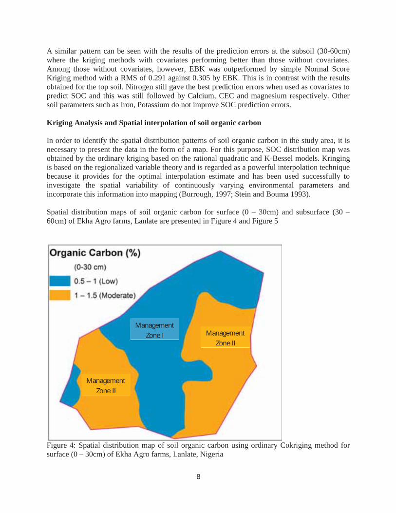
A similar pattern can be seen with the results of the prediction errors at the subsoil (30-60cm) where the kriging methods with covariates performing better than those without covariates. Among those without covariates, however, EBK was outperformed by simple Normal Score Kriging method with a RMS of 0.291 against 0.305 by EBK. This is in contrast with the results obtained for the top soil. Nitrogen still gave the best prediction errors when used as covariates to predict SOC and this was still followed by Calcium, CEC and magnesium respectively. Other soil parameters such as Iron, Potassium do not improve SOC prediction errors. Kriging Analysis and Spatial interpolation of soil organic carbon In order to identify the spatial distribution patterns of soil organic carbon in the study area, it is necessary to present the data in the form of a map. For this purpose, SOC distribution map was obtained by the ordinary kriging based on the rational quadratic and K-Bessel models. Kringing is based on the regionalized variable theory and is regarded as a powerful interpolation technique because it provides for the optimal interpolation estimate and has been used successfully to investigate the spatial variability of continuously varying environmental parameters and incorporate this information into mapping (Burrough, 1997; Stein and Bouma 1993). Spatial distribution maps of soil organic carbon for surface (0 – 30cm) and subsurface (30 – 60cm) of Ekha Agro farms, Lanlate are presented in Figure 4 and Figure 5

Figure 4: Spatial distribution map of soil organic carbon using ordinary Cokriging method for surface (0 – 30cm) of Ekha Agro farms, Lanlate, Nigeria

Management Zone II

Management Zone I

Management Zone II

9

Table 4: Cross validation prediction error parameters for different Kriging methods (covariates are in bracket for Cokriging methods)

0-30 cm depth

Empirical Bayesian Kriging (EBK)

Ordinary Kriging

Universal Kriging

Simple Normal Score Kriging

Ordinary Cokriging (Nitrogen)

Simple Normal Cokriging (Nitrogen)

Simple Normal Cokriging (Calcium)

Simple Normal Cokriging (CEC)

Simple Normal Cokriging (Magnessium)

Ordinary Cokriging (NDVI)

Simple Normal Cokriging (EVI)

Mean error (ME) -0.0114 -0.0004 -0.0004 -0.0043 -0.0053 -0.0034 -0.0058 -0.0057 -0.0051 -0.0010 -0.0045

Root Mean Square Error (RMS) 0.3221 0.3298 0.3298 0.3298 0.2383 0.2311 0.2640 0.2681 0.2877 0.3288 0.3287

Mean Standard Error (AVS) 0.3120 0.3227 0.3196 0.3100 0.2351 0.2069 0.2532 0.2573 0.2708 0.3230 0.3098

Root Mean Square Standardized (RMSS) 1.0170 1.0101 1.0321 1.0578 0.9989 1.0706 0.9795 0.9857 1.0220 1.0087 1.0479

Model Type Hole

Effect Hole

Effect Hole

Effect K-Bessel K-Bessel Stable Stable Stable Hole

Effect Hole

Effect

30-60cm depth

Mean error (ME) 0.0006 0.0001 -0.0014 0.0115 -0.0062 -0.0070 -0.0013 0.0017 0.0049 0.0026 0.0039

Root Mean Square Error (RMS) 0.3051 0.3201 0.3183 0.2912 0.2153 0.1999 0.2649 0.2744 0.2896 0.3026 0.3050

Mean Standard Error (AVS) 0.3041 0.2998 0.3128 0.2804 0.2580 0.1908 0.2482 0.2587 0.2623 0.2943 0.3005

Root Mean Square Standardized (RMSS) 0.9796 1.0660 1.0167 1.0067 0.9773 1.0912 1.0001 1.0080 1.0592 1.0021 1.0011

Model Type J-Bessel Hole

Effect J-Bessel J-Bessel Stable K-Bessel K-Bessel Rational

Quadratic Hole

Effect Gaussian

10

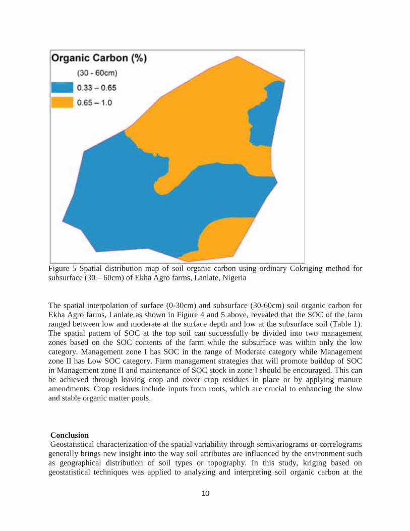
Figure 5 Spatial distribution map of soil organic carbon using ordinary Cokriging method for subsurface (30 – 60cm) of Ekha Agro farms, Lanlate, Nigeria The spatial interpolation of surface (0-30cm) and subsurface (30-60cm) soil organic carbon for Ekha Agro farms, Lanlate as shown in Figure 4 and 5 above, revealed that the SOC of the farm ranged between low and moderate at the surface depth and low at the subsurface soil (Table 1). The spatial pattern of SOC at the top soil can successfully be divided into two management zones based on the SOC contents of the farm while the subsurface was within only the low category. Management zone I has SOC in the range of Moderate category while Management zone II has Low SOC category. Farm management strategies that will promote buildup of SOC in Management zone II and maintenance of SOC stock in zone I should be encouraged. This can be achieved through leaving crop and cover crop residues in place or by applying manure amendments. Crop residues include inputs from roots, which are crucial to enhancing the slow and stable organic matter pools. Conclusion Geostatistical characterization of the spatial variability through semivariograms or correlograms generally brings new insight into the way soil attributes are influenced by the environment such as geographical distribution of soil types or topography. In this study, kriging based on geostatistical techniques was applied to analyzing and interpreting soil organic carbon at the

11

surface (0-30cm) and subsurface (30-60cm) depths in a commercial cassava farm at Lanlate, southwestern, Nigeria. The analysis of the spatial structure showed that SOC at both depths were spatially correlated. SOC was generally higher at the topsoil than at subsoil. Covariates such as Nitrogen, Calcium, CEC and Magnesium improved prediction errors thereby making for more reliable predictions. The spatial distribution of soil organic carbon at Ekha farm is dominated by the constitutive factors and the random factors together. The background content, type of soil forming mineral and soil type are the main aspects of the constitutive factors and human activities such as tillage-cropping systems, management measures, wastewater irrigation, vegetation cover, manure, crop residue management and artificial pollution are the random factors. Because of the disruptions and influences by human activities, the spatial relationship of soil organic carbon in the study area was weakened. However based on the spatial interpolation of the SOC, two management zones were delineated for the surface depth. Farm management strategies that will promote buildup of SOC in Management zone II and maintenance of SOC stock in zone I should be encouraged. References AfSIS, 2014: Africa Soil Information Service (AfSIS). http://www.africasoils.net/data/datasets Burrough, P.A. 1997. Principles of Geographical Information Systems, pp. 132-137. Oxford University Press.

Burrough, P.A. and McDonnell, R.A. 1998. Principals of Geographical Information Systems. Oxford, UK: Oxford University Press.

Cambardella C.A,., T.B. Moorman, T.B. Parkin, D.L. Karlen, R.F. Turco, and A.E. Konopka.. Field scale variability of soil properties in Central Iowa soils. Soil Sci. Soc. Am. J. 58:1501–1511. 1994 Chien Y. J., Lee D. Y., Guo H. Y & Houng K. H. (1997). Geostatistical analysis of soil properties of mid-west Taiwan soils. Soil Science, 162, pp. 291–298. Cleared Land. Soil Science Society of America Journal 51, 668-674.

CSIRO, 2011 Soil carbon: The Basics http://www.csiro.au/Outcomes/Environment/Australian-Landscapes/soil-carbon.aspx

McGrath D,. C. S. Zhang, and O. T. Carton, Geostatistical analyses and hazard Assessment on soil lead in Silvermines area, Ireland. Environmental Pollution. vol,127, 2004. pp.239-248 Ersoy A, T.Y. Yunsel,., M Cetin,. Characterization of land contaminated by heavy metal mining using geostatistical methods. Archives of Environmental Contamination and Toxicology. vol, 46, 2004, pp.162- 175.

12

Flowers, M., R. Weisz, and J.G. White. 2005. Yield-based management zones and grid sampling strategies: describing soil test and nutrient variability. Agron. J. 97:968-982.

Gallardo A.,. Spatial variability of soil properties in a floodplain forest in northwest Spain. Ecosystems. vol, 6,2003, pp. 564- 576. 2003 Goovaerts, P. (1997) Geostatistics for Natural Resources Evaluation. Oxford University Press, Oxford.. Lark R. M. (2002). Optimized spatial sampling of soil for estimation of the variogram by maximum likeliwood. Geoderma, 105, pp. 49–80.

Leeper, GW and Uren, NC (1993) 5th edn, Soil science, an introduction, Melbourne University Press, Melbourne

Leu, A (2007). Organics and soil carbon: increasing soil carbon, crop productivity and farm profitabilit in ‘Managing the Carbon Cycle’ Katanning Workshop 21-22 March 2007 www.amazingcarbon.com Miller M. P., Singer P. M. J. & Nielse, D. r. (1988). Spatial variability of wheat yield and soil properties on complex hills. SSSAJ, 52, pp. 1133–1141. Nielsen, D.R. and Wendroth, O. (2003) Spatial and temporal statistics: Sampling field soils

andTheir vegetation. Reiskirchen, Catena Verlag, 2003. 398p. Patil, S.S., V.C. Patil and K.A. Al-Gaadi 2011 Spatial Variability in Fertility Status of Surface Soils; World Applied Sciences Journal 14 (7): 1020-1024, 2011 ISSN 1818-4952 © IDOSI Publications, 2011

Santra, P., V.K. Chropra and D. Chakraborty, 2008 Spatial variability of soil properties and its application in predicting surface map of hydraulic parameters in an agricultural farm. Curr. Sci., 95(7): 937-945.

Schimel, D.S., 1995. Terrestrial ecosystems and the carbon cycle. Global Change Biology 1, 77–91. Schlesinger, W. H. (1977) Carbon balance in terrestrial detritus. Annual Review of Ecology and Systematics, 8,51-81.

Sonneveld B.G. J.S, 2005. Compilation of a soil map of Nigeria: A nation-wide soil resource and landform inventory. Nig. J. Soil Res. Vol. 6: 2005 71 – 83 Stein, A., Bouma, J. 1. Methods for comparing spatial variability patterns of millet yield and soil data. Soil Science Society of America Journal.vol,61, 1997, pp.861-870.

13

Trangmar, B. B., R. S. Yost, M. K. Wade, G. Uehara, and M. Sudjadi, 1987. Spatial Variation of Soil Properties and Rice Yield on Recently Cleared Land. Soil Science Society of America Journal 51, 668-674. Voltz, M.,Webster, R., 1990. A comparison of kriging, cubic splines and classification for predicting soil properties from sample information. J. Soil Sci. 41, 473–490. Walkley, A. and I.A. Black, (1934). An examination of the Degtjareff method for determining

soil organic matter and a proposed modification of the chromic acid titration method. Soil Sci. 37

Webster, R., Oliver, M. A (1990). Statistical methods in soil and land resource survey. Oxford University Press, Oxford Yost, R.S., G. Uehara and R.L. Fox, 1982. Geostatistical analysis of soil chemical properties of large land areas. i. semi-variograms. Soil Sci. Soc. Am. J., 46: 1028-1032

Young, A and Young, R. (2001). Soils in the Australian landscape. Melbourne: Oxford University Press. ISBN 978-0-19-551550-3.