spatial topology and its structural analysis based on the

Transactions in GIS

, 2007, 11(6): 943–960

© 2007 The Authors. Journal compilation © 2007 Blackwell Publishing Ltd

Blackwell Publishing LtdOxford, UKTGISTransactions in GIS1361-1682© 2008 The Authors. Journal compilation © 2008 Blackwell Publishing LtdXXX Original Articles

Spatial Topology and its Structural AnalysisB Jiang and I Omer

Research Article

Spatial Topology and its Structural Analysis based on the Concept of Simplicial Complex

Bin Jiang

Department of Land Surveying and Geo-InformaticsHong Kong Polytechnic University

Itzhak Omer

Environmental Simulation LaboratoryDepartament of Geography and Human EnvironmentTel-Aviv University

Abstract

This paper introduces a model that identifies spatial relationships for structuralanalysis based on the concept of simplicial complex. The spatial relationships areidentified through overlapping two map layers, namely a primary layer and acontextual layer. The identified spatial relationships are represented as a simplicalcomplex, in which simplices and vertices, respectively, represent two layers of objects.The model relies on the simplical complex for structural representation and analysis.To quantify structural properties of individual primary objects (or equivalentlysimplices), and the simplicial complex as a whole, we define a set of centralitymeasures by considering multidimensional chains of connectivity, i.e. the number ofcontextual objects shared by a pair of primary objects. With the model, the interactionand relationships with a geographic system are modeled from both local and globalperspectives. The structural properties and modeling capabilities are illustrated by asimple example and a case study applied to the structural analysis of an urbansystem.

1 Introduction

The first law of geography nicely describes an important characteristic of geographicsystems in which “everything is related to everything else, but near things are more relatedthan distant things” (Tobler 1970). The law suggests an overall structure of any geographicsystem, i.e. near things are more related than distant things. This is indeed true, as

Address for correspondence:

Bin Jiang, Department of Land Surveying and Geo-Informatics, TheHong Kong Polytechnic University, Kowloon, Hong Kong. Email: [email protected]

944

B Jiang and I Omer


Transactions in GIS

, 2007, 11(6)

spatial phenomena are not random. More significantly, the law implies an underlyingnetwork view as to how “things” are interconnected. This network view is oftenrepresented as a graph in which the “things” are vertices and thing-thing relationshipsare edges. This can be seen clearly from the well known TIGER data model. Underthe data model, linear objects form a kind of network in conventional quantitative geography(Haggett and Chorley 1969) and transportation modelling (Miller and Shaw 2001).Based on the geometric network representation, a series of network analyses can becarried out such as geocoding and routing analysis. A street network can also beperceived from a purely topological perspective (Jiang and Claramunt 2004), withwhich some universal patterns can be illustrated (e.g. Jiang 2007). In fact, the networkanalysis can be extended to all types of objects in Geographic Information Systems(GIS), as long as a rule of relationship is given for setting up an interconnected relationshipor topology. Current GIS, mainly based on a geometric paradigm, have not yet adoptedthe topological paradigm for advanced spatial analysis (Albrecht 1997, Batty 2005),particularly in the context of the emerging science of networks (Barabási 2003, Watts2004) following the two seminal papers (Watts and Strogatz 1998, Barabási and Albert1999). Furthermore, most of the existing studies adopted a graph theoretic approach forsetting up networks, and the thing-thing relationships are constrained by a direct relationship.For instance, two disjoint areas are usually considered to have no relationships.

This article describes a model that can help to set up thing-thing relationships (forthings which have no obvious direct relationships), in order to explore structural propertiesof individual objects of a geographic system, as well as the geographic system as a whole.Distinct from previous studies mostly based on graph theory for network representation,this article adopted the concept of simplicial complex, as defined in the theory of Q-analysis(Atkin 1974), for the representation and structural analysis of geographic systems.The structural analysis is fundamental to understanding the flows of goods, informationand people within a geographic system. Although Q-analysis shares with graph theory somesimilarity in terms of topology (Earl and Johnson 1981), the simplicial complex represen-tation is capable of exploring structural properties from the perspective of multidimensionalchains of connectivity. In this article, we direct our attention to an overall structure or topologyof an entire geographic system, and to how various parts (or objects) of the geographicsystem interact. In other words, our modeling effort is to take the interrelationship ofspatial objects as a whole and explore its structure at both local and global levels.

Q-analysis, initially developed from algebraic topology and by Atkin (1974, 1977),is a set theoretic method to set up relationships of two sets and further explore thestructure of the relationships. It provides a computational language for structuraldescription using both geometric and algebraic representations. Because of its capabilityin structural description, Q-analysis has been used to explore man-environment interactions,ecological relations, and urban structure in social science, geography, and urban studies(Gould 1980). Recently, Q-analysis has also found some interesting applications incomplexity study (Degtiarev 2000), database structure (Kevorchian 2003) and economicstructure analysis (Guo et al. 2003). To the best of our knowledge, Q-analysis has notbeen applied to spatial analysis in GIS, in particular in the way we suggest in this article.We believe that the model we suggest in this article can provide unique insights into thestructure of various geographic systems through layered geographic information – acommon data format of existing GIS.

The remainder of this article is organized as follows. Section 2 introduces spatialtopology that is a network representation of spatial relationships within a geographic

Spatial Topology and its Structural Analysis

945


Transactions in GIS

, 2007, 11(6)

system. Section 3 presents how Q-analysis in general and simplicial complex in partic-ular can be used to characterize structural properties of a spatial topology. Section 4suggests three centrality measures to characterize structural properties of individualobjects within a geographic system. The introduced model and measures are applied toa case study for topological analysis of an urban system in section 5. Finally, section 6concludes the paper and points out possible future work.

2 Spatial Topology: Definition and Illustration

Here we introduce a model to identify spatial relationships of geographic objects viacommon objects. To introduce the model, let us start with an example from socialnetworks. Two persons, A and B, are not acquainted in a general social sense as colleaguesor friends, but they can be considered as “adjacent”, as both, for instance, belong to thesame geographic information community. The community or organization peoplebelong to is a context that keeps people “adjacent”. Extending the case into a geographiccontext, we can say that, for instance, two houses are adjacent if they are both situatedalong the same street, or within the same district. We can further state that a pair ofobjects sharing more common objects is more “adjacent”. Now let us turn to the formalmodel for identifying such spatial relationships. The model aims to represent spatialrelationships of various objects as a simplicial complex. To this end, some formal defi-nitions are also presented in the context of GIS.

2.1 Defining Spatial Topology

We start with a definition of map layer according to set theory. Map layer is defined asa set of spatial objects at a certain scale in a database or on a map. For example,

M

=

{

o

1

,

o

2

, . . . ,

o

n

}, or

M

=

{

o

i

|

i

=

1, 2, . . . ,

n

} denotes a map layer (using a capital letter)that consists of multiple objects (using small letters). The objects can be put into fourcategories: point, line, area, and volume objects in terms of basic graphic primitives.Note that the definition of objects must be appropriate with respect to the modelingpurpose. For instance, a street layer can be considered a set of interconnected streetsegments, or an interconnected named street depending on the modeling purpose (Jiangand Claramunt 2004); a city layer can be represented as a point or area object depend-ing on the representation scale.

A spatial topology (

T

) is defined as a subset of the Cartesian product of two maplayers,

L

and

M

, denoted by

T

=

L

×

M.

To set up a spatial topology, we need toexamine the relationship of every pair of objects from one map layer to another. Asdistinct to topological relationships based on possible intersections of internal and exter-nal boundaries of spatially extended objects (Egenhofer 1991), we simply take a binaryrelationship. That is, if an object

�

is within, or intersects, another object

m

, we saythere is a relationship

λ

=

(

�

,

m

), otherwise no relationship,

λ

=

φ

[Note: the pair(

�

,

m

) is ordered, and (

m

,

�

) represents an inverse relation denoted by

λ

−

1

]. The relation-ship can be simply expressed as “an object has a relationship to a contextual object”. Ifa set of primary objects shares a common contextual object, we say the set of objectsare adjacent or proximate. Thus two types of map layers can be distinguished: theprimary layer for the primary objects, with which a spatial topology is to be explored,and the contextual layer, whose objects constitute a context for the primary objects. It

946

B Jiang and I Omer


Transactions in GIS

, 2007, 11(6)

is important to note that the contextual layer can be given in a rather abstract way witha set of features (instead of map objects). This way, the relationship from the primaryto contextual objects can be expressed as “an object has certain features”. For the sakeof convenience and with notation

T

=

L

×

M

, we refer to the first letter as the primarylayer and the second the contextual layer.

The notion of spatial topology presents a network view as to how the primaryobjects become interconnected via the contextual objects. A spatial topology can berepresented as a simplicial complex. Before examining the representation, we turn to thedefinition of simplicial complex (Atkin 1977). A simplicial complex is the collection ofrelevant simplices. Let us assume the elements of a set

A

form simplices (or polyhedra,denoted by

σ

d

where d is the dimension of the simplex); and the elements of a set

B

form vertices according to the binary relation

λ

, indicating that a pair of elements (

a

i

,

b

j

) from the two different sets

A

and

B

,

a

i

∈

A

and

b

j

∈

B

, are related. The simplicalcomplex can be denoted as

K

A

(

B

;

λ

). In general, each individual simplex is expressed asa

q-

dimensional geometrical figure with

q

+

1 vertices. The collection of all the simplicesforms the simplicial complex. For every relation

λ

it is feasible to consider the conjugaterelation,

λ

−

1

, by reversing the relations between two sets

A

and

B

by transposing theoriginal incidence matrix. The conjugate structure is denoted as

K

B

(

A

;

λ

−

1

).A spatial topology can be represented as a simplicial complex where the simplices

are primary objects, while vertices are contextual objects. Formally, the simplicial com-plex for the spatial topology

T

=

L

×

M

is denoted by

K

L

(

M

; λ), where L represents theprimary layer, and M the contextual layer, the relation between a primary object andcontextual object λ = (�, m). A spatial topology can be represented as an incidencematrix Λ, where the columns represent objects with the primary layer and the rowsrepresent the objects with the contextual layer. Formally it is represented as follows:

(1)

The entry 1 of the matrix indicates that a pair of objects (i, j) respectively from the twodifferent layers L and M (i.e. i ∈ L and j ∈ M) is related, while the entry 0 representsno relationship between the pair of the objects. The incidence matrix Λij is not symmetric,as λ ≠ λ−1 in general.

Spatial topology is not intended to replace the existing topology or spatial relation-ship representation, but to extend and enhance the existing ones for more advancedspatial analysis and modelling. In this respect, the simplicial complex representationprovides a powerful tool for exploring structural properties of spatial topology. Beforeintroducing the structural analysis, we take a look at a simple example.

2.2 A Simple Example

Let us assume with environmental GIS, three pollution sources whose impact areas areidentified, through a buffer operation, as a polygon layer. It is likely that the threepolluted zones overlap each other. This constitutes a map layer, denoted by Y = (yj | j =1, 2, 3). To assess the pollution impact on a set of locations with another map layerX = (xi | i = 1, 2, . . . 6), it is not sufficient to just examine which location is within whichpollution zones. We should take a step further to put all locations within an interconnectedcontext (a network view) using the concept of spatial topology. For instance, locationx1 is out of pollution zone y2, but it may get polluted through x2 and x5, assuming the

Λijif i jif

: ( , ) :

= =⎧⎨⎩10

λφ

Spatial Topology and its Structural Analysis 947

© 2007 The Authors. Journal compilation © 2007 Blackwell Publishing LtdTransactions in GIS, 2007, 11(6)

kind of pollution is transmittable. Only under the network view are we able to investigatethe pollution impact thoroughly.

In the example, the locations under pollution impact are of primary interest.Using Equation (1), the spatial topology can be represented as an incidence matrix asfollows.

For the primary layer, the six locations in Figure 1 and with respect to the columns ofthe matrix can be represented as six simplices as follows:

σ0(x1) = <y1>

σ1(x2) = <y1, y2>

σ1(x3) = <y2, y3>

σ0(x4) = <y3>

σ2(x5) = <y1, y2, y3>

σ0(x6) = <y3>

where the right hand side of the equation represents vertices that consist of a givensimplex. The dimension of a simplex is represented by a superscript. For instance, σ2(y5)denotes a 2-dimensional simplex or a 2-dimensinal face that consists of three vertices y1,y2, and y3. The simplices and the related complex can be graphically represented as inFigure 2.

Note that the primary and contextual objects are relative and transversal (inter-changeable) depending on different application interests. If for instance we take Y as theprimary layer (whether it makes sense is another issue which we will not consider here),i.e. to transpose the incidence matrix defined in Equation (1), then we would have threesimplices as follows (see also Figure 3a):

Λ36

1 2 3 4 5 6

1

2

3

1 1 0 0 1 00 1 1 0 1 00 0 1 1 1 1

=

⎡

⎣

⎢⎢⎢⎢

⎤

⎦

⎥⎥⎥⎥

x x x x x xyyy

Figure 1 A simple example

948 B Jiang and I Omer


σ2(y1) = <x1, x2, x5>

σ2(y2) = <x2, x3, x5>

σ3(y3) = <x3, x4, x5, x6>

The collection of the three simplices constitutes a three-dimensional complex (Figure 3b).We have noted that a spatial topology can be represented as a geometric form (the

simplicial complex). It is important to note that the geometric representation makes littlesense when the dimension of the simplicial complex exceeds three because of a humanperceptual constraint, but there is no such constraint for the algebraic approach. In this article,we mainly concentrate on the algebraic approach for structural analysis of a spatial topology.

3 Structural Properties of a Spatial Technology

A spatial topology can be represented as a connected simplicial complex for structuralanalysis based on Q-analysis theory. In this case, primary objects are represented as

Figure 2 The six simplices (a) and their collection – the simplicial complex Kx(Y; λ ) (b)

Figure 3 The three simplices (a) and their collection – the simplicial complex Ky (X; λ −1) (b)



individual simplicies, with contextual objects as the vertices of simplices. For theprimary layer, a pair of objects can be assessed to see if they share a common contextualobject, and if so, how many common objects they share. If there are q + 1 commoncontextual objects shared, we say the pair of primary objects is q-near. For example,0-nearness means that a pair of primary objects shares one contextual object, and1-nearness means 2 contextual objects are shared. For the example in Figure 3, the pairy1 − y2 shares two objects, i.e. two vertices x2 and x5, so we say y1 and y2 are 1-near. If,on the other hand, there is no contextual object shared, i.e. −1-near, but each of theprimary objects is q-near one or several common primary objects, we say that the pair ofobjects is q-connected due to the transitive rule. For instance, the primary objects y1 andy3 have only one common contextual object (x5), but they are 1-connected due to theprimary object y2 that serves as a transitional object; y2 is 1-near with y1 and with y3. Ina more general way, we say that two objects are q-connected if they are q-near or thereis a chain of q-near simplices between them. That is, two objects can be connectedthrough more than one transitional simplex (this is true of course for a case where thereis more than three primary objects). As a general rule, two simplices are q-near, theywould be also q-connected, but not vice versa.

The Q-analysis is based on the q-nearness and q-connectivity relations between thesimplices of a given complex (or simplicial complex). A Q-analysis of a complex KL(M; λ)determines the number (#) of distinct equivalence classes, or q-connected components,for each level of dimension q ranging from 0 to q − 1. The equivalence classes aredetermined by a rule as follows. If two simplices are q-connected (either q-near or q-connected), then they are in the same class. For example, the Q-analysis of the complexin Figure 3 leads to the following equivalence classes at the different dimensional levels ofq = 0, q = 1, q = 2 and q = 3. Each equivalence class is enclosed in the curly brackets below:

q = 0: {y1, y2, y3}

q = 1: {y1, y2, y3}

q = 2: {y1}, {y2}, {y3}

q = 3: {y3}

The spatial topology can be analyzed by Q-analysis from a global perspective. That is,through counting the number of components at each q-level, we are able to get a structurevector Q. It is defined as follows:

(2)

where the superscripts of the structural vector denote the dimension q, i.e. 0, 1, 2, . . . ,(q − 1) from right to left. Large entries in Q indicate that the structure at a certaindimension is fragmented or disconnected, while small entries imply more integrity structure.

For instance, the structure vector for the complex in Figure 3 indicates thatthere is one equivalence class (EC) at dimensional zero, one EC at dimension one, threeECs at dimension two, and one EC at dimension three. In other words, the complex israther fragmented at the second dimension, and rather integrated at the zero, first andthird dimensions. Such an analysis can provide some critical insights into the structureof a spatial topology in terms of information flows.

From a local perspective we could assess the uniqueness of individual primaryobjects in the whole spatial topology by the eccentricity index. This index is defined by

Q qq {# # # # } . . .

. . . = −−11

22

11

00

Q { }= 1 3 1 13 2 1 0



the relation between a dimension where an object is disconnected and another dimensionwhere the object is integrated. It is formally expressed as follows:

(3)

where œ or top-q denotes the highest dimension of the simplex (σi); q or bottom-q denotesthe lowest q level where the simplex gets connected to any other simplex. The eccentricityvalues of the primary objects in the complex presented in Figure 3 are Ecc (y1) = 0.5,Ecc (y2) = 0.5, and Ecc (y3) = 1.

According to Equation (3), a primary object (as a simplex) gains a high value ofeccentricity if it is different from every other. Thus it differentiates other simplices in thesense of uniqueness, rather than in the sense of importance or function in the flows andtransmission within a complex. In other words, the eccentricity cannot preciselycharacterize the status of different simplices. This can be illustrated with the complexshown in Figure 3, where both simplices y1 and y2 have the same eccentricity value (0.5).However, it is intuitive enough that y2 tends to be more important structurally than y1.Referring to the complex in Figure 3, without y2, the complex would be broken into twopieces at dimension two, while y2 and y3 are still kept together with the loss of y1. Thereason for this stems from the fact that the status of y2, as a transitional simplex inthe equivalence classes of dimensions of 0 and 1, is not taken into consideration inthe eccentricity computation. In other words, the computation of eccentricity doesnot consider nearness relations within the equivalence class, but such relations arecritical in determining the status of a simplex.

4 New Measures for Characterizing Structural Properties of Individual Simplices

The inability of eccentricity to describe the status of individual simplices within acomplex enables us to seek alternative measures for it. Centrality measures initiallydeveloped in the field of social networks (Freeman 1979) aim to support the quantitativedescription of a node status within a graph. It consists of three separate measurescharacterizing centrality from different perspectives: degree, closeness and betweenness.The degree centrality describes how many other nodes are connected directly to aparticular node. It can be obtained by simply counting the number of directly linkednodes. The closeness quantifies how close a node is to every other node by computingthe shortest distances from every node to every other. The betweenness measures towhat extent a node is located in between the paths that connect pairs of nodes, and assuch it reflects directly the intermediary location of a node along indirect relationshipslinking other nodes. We have extended the centrality measures into a simplicial complexto characterize the status of individual simplices within the complex. Basically, wedefine each measure at different dimensional levels, and then sum them up to show thecentrality of individual simplices.

4.1 Degree Centrality

For describing the degree centrality of a given simplex within a complex, we mustillustrate how many other simplices are directly connected to the simplex. We need to

Ecc i( )

σ =−+

œ qq 1



define the measure for a simplex at a different dimensional level. For a simplex (σi), thedegree centrality at a given dimension level q can be formulated as follows:

(4a)

where n is the total number of simplices within a complex, and λq denotes whether thereis direct relation (λ) between simplex (σi) to another simplex (σk) at dimension q.

To describe the overall degree centrality of a simplex within a simplicial complex,i.e. the total degree centrality of a simplex of different dimensions, we must accumulatethe degrees at the different dimensions, i.e.

(4b)

where max(q) represents the highest level of dimension of the complex. Thus, the totaldegree centrality indicates to what extent a simplex is connected directly in the wholecomplex.

4.2 Closeness Centrality

The closeness centrality in a graph context aims to assess the status of a node within agraph. It examines how a node is integrated or segregated with a graph or network. Itis interesting that the measure has different names in different contexts. For instance, itis called status in graph theory (Buckley and Harary 1990), whereas in space syntaxit is called integration (Hillier and Hanson 1984), computed from the reciprocal value ofpath length, a key concept used in small world theory (Watts and Strogatz 1998). Basedon the idea of closeness centrality, we suggest here a similar measure to quantify howeach simplex is close to every other. We define the measure for a simplex within acomplex at the different dimensional level.

(5a)

where d is the shortest distance from a given simplex (σi) to every other simplex, n isthe total number of simplices within a complex. Note the measure is given at a dimensionallevel q. Or put differently, the computation of the closeness considers multidimensionalchains of connectivity. A simplex gains a closeness value at the different dimensionallevel if it gets connected to other simplices.

Logically the closeness measure can be accumulated along the different dimensionallevels, to show an overall closeness of a simplex to every other at various dimensionallevels. The accumulated closeness can be formulated as follows:

(5b)

where max(q) represents the highest level of dimension of the complex.

D qi q i kk

n

( ) ( , )σ λ σ σ==

∑1

D qi i kk

n

q

q

( ) ( , )max( )

σ λ σ σ===

∑∑11

Cn

di q

i kk

n( )

( , )

σσ σ

=−

=∑

1

1

Cn

di

i kk

nq

q

( )

( , )

max( )

σσ σ

=−

=

= ∑∑ 1

1

0



4.3 Betweenness Centrality

On the basis of the idea of betweenness centrality, we suggest here a similar measure fordescribing the linkage status of a simplex within a complex. Unlike the betweennesscentrality in graph theory where the analysis focuses on zero-dimensional links using aterm in q-analysis, we consider the multidimensional nature of the linkage. That is, towhat extent a simplex is located in between the paths that connect pairs of simplices inthe simplical complex at different dimensional levels and thereby determine thebetweenness centrality of a given simplex at all dimensions. Accordingly, we definebetweenness centrality for a simplex (σi) in a given dimension q as follows:

(6a)

where Pij denotes the number of shortest paths between simplices σi and σj, and Pikj isthe number of shortest paths from σi to σj that pass through transitional simplex σk, i.e.the simplices σi and σj are q-connected by the transitional simplex σk; Pikj is a binaryvalue that indicates if a simplex σk serves as a transitional simplex for σi and σj – if so,Pikj = 1, otherwise Pikj = 0. Hence, the transitive weight of each transitional simplex σk

for a given pair σiσj is equal to the proportion 1/Pij i.e. if there is only one minimumpath between i and j then σk gains the value 1; if there are two minimum paths σk gainsthe value 1/2. Accordingly, the betweenness centrality of a simplex σk at dimension levelq is equal to the cumulative transitive weight values of σk for all the pairs at thatdimension. Note: the betweenness value does not exist when Pij = 0.

Applying the computation of B(σi)q for all the dimensions where the simplex isconnected to other simplices defines the total betweenness centrality of the simplexwithin a complex K:

(6b)

where max(q) represents the highest level of dimension of the complex. The total centralitymeasure is a cumulative value obtained by applying the computation of B(σi)q frombottom-q (the highest dimension at which a simplex gets connected to other simplices)down to dimension 0. As its counterpart defined in graph theory, this measure indicatesto what extent a simplex is important for the linkage within a complex. If a simplexwith higher value of betweenness gets removed, the whole complex may get broken intopieces.

5 Structural Analysis of an Urban System: Case Study

We applied the introduced model and measures to the city of Tel Aviv in Israel forstudying park-park and neighborhood-neighborhood relationships – a kind of structuralanalysis of urban systems. To achieve this goal, we first adopt neighborhoods as thecontextual layer to assess the park-park relationships. That is, two parks are inter-related if the two are accessible by some neighborhoods. Depending on the number ofneighborhoods, the strength of relationship varies from one pair to another, thusproviding a kind of multiple chain of connectivity among the parks. In the case study,a layer of 46 parks (0–45), denoted by P, and a layer of 62 neighborhoods (0–61),

BP

Pi q

ikj

ijji

( ) σ = ∑∑

BP

Pi

ikj

ijjiq

q

( ) max( )

σ = ∑∑∑=0



denoted by N, are overlapped (Figure 4), create the simplical complex Kp(N; λ) to assesswhether a park is accessible by a neighborhood. It should be noted that parks aredefined as green areas larger than 20,000 m2, and a park is accessible by a neighborhoodif it is within 0.5 km radius from the border of the park (these kinds of criteria are

Figure 4 Parks and neighborhoods in Tel-Aviv



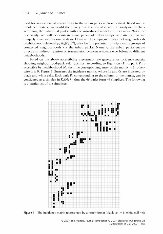
used for assessment of accessibility to the urban parks in Israeli cities). Based on theincidence matrix, we could then carry out a series of structural analysis for char-acterizing the individual parks with the introduced model and measures. With thecase study, we will demonstrate some park-park relationships or patterns that areuniquely illustrated by our analysis. However the conjugate relation, of neighborhood-neighborhood relationship, KN(P; λ−1), also has the potential to help identify groups ofconnected neighborhoods via the urban parks. Namely, the urban parks enabledirect and indirect relation or transmission between residents who belong to differentneighborhoods.

Based on the above accessibility assessment, we generate an incidence matrixshowing neighborhood-park relationships. According to Equation (1), if park Pi isaccessible by neighborhood Nj, then the corresponding entry of the matrix is 1, other-wise it is 0. Figure 5 illustrates the incidence matrix, whose 1s and 0s are indicated byblack and white cells. Each park Pi, corresponding to the column of the matrix, can beconsidered as a simplex in Kp(N; λ), thus the 46 parks form 46 simplices. The followingis a partial list of the simplices:

Figure 5 The incidence matrix represented by a raster format (black cell = 1, white cell = 0)



σ6(P0) = <N35, N37, N38, N39, N41, N42, N43>

σ4(P1) = <N43, N47>

. . .

σ5(P44) = <N1, N2, N3, N4, N6, N7>

σ0(P45) = <N1>

Obviously some simplices can be represented geometrically as a tetrahedron, while mostothers have the dimension of more than three. The higher dimensional simplices ifrepresented geometrically are difficult to perceive by human beings in terms of thecomplexity of structure, particularly for a large system. In this case, the algebraicmethod of spatial topology shows an advantage in discovering structure from both localand global perspectives.

We then rely on the incidence matrix for Q-analysis, forming the connected com-ponents (or EC as previously mentioned) at different dimensions (see Table 1, whereeach component is enclosed by curly brackets). It is intriguing to note from the tablethat all the simplices at dimension zero (q = 0) are interconnected, forming one inter-connected component. In contrast, the simplices are fragmented into two isolated partsat dimension one (q = 1). Furthermore at dimension one, there are two interconnectedcomponents: the first containing 43 simplices, and second containing 2 simplices. Interms of Q-analysis, simplices within each component are either q-near or q-connected.For the biggest component at dimension one, it means that all the simplices within thecomponent are 1-connected. The resulting connected components have far-reachingimplications in terms of structural analysis. From the structural perspective, the sim-plices at dimension one are not interconnected as a whole as at dimension zero. How-ever, the interconnected components at dimension one tend to trade more flows amongthe individuals. Taking the pair of parks {1, 4} for example, it has two neighborhoodsaccessible to the pair. In a similar fashion, the two pairs {0, 2}, {27, 30} at dimensiontwo (q = 2) have stronger interaction since they have three neighborhoods accessible

Table 1 Q-analysis of the park-park relationship (Note: connected components are highlighted)

q = 0: {0,1,2,3,4,5,6,7,8,9,10,11,12,13,14,15,16,17,18,19,20,21,22,23,24,25,26,27,28,29,30,31,32,33,34,35,36,37,38,39,40,41,42,43,44,45}

q = 1: {0,2,3,5,6,7,8,9,10,11,12,13,14,15,16,17,18,19,20,21,22,23,24,25,26,27,28,29,30,31,32,33,34,35,36,37,38,39,40,41,42,43,44} {1,4}

q = 2: {0,2} {3,6,8,9} {4} {5} {7} {10,11,13} {12,14,16} {15} {17} {18} {20,21,25,32,34,36,38,40,41,43,44} {22} {26} {27,30} {31,33,35,37}

q = 3: {0,2} {3,6} {4} {5} {7} {8} {9} {10} {11} {12,14} {13} {15} {16} {18} {21} {22} {25,34,44} {30} {31,33,37} {36} {40}

q = 4: {0,2} {3} {5} {6} {8} {9} {12} {13} {14} {21} {30} {31,33,37} {34} {44}q = 5: {0,2} {3} {6} {12} {13} {14} {21} {30} {33} {44}q = 6: {0,2} {21}q = 7: {2}

Q { }= 1 2 10 14 21 15 2 17 6 5 4 3 2 1 0



to each other. This kind of information is certainly unique to the multidimensionaltopological analysis suggested here. As such, this approach can be considered as anadvantage in comparison to the traditional network analysis which did not considerthe multidimensional chain of connectivity.

The structural vector according to Equation (2) indicatesthe degree of integration or fragmentation at different dimensions for the individualparks. The results of the above analysis are mainly carried out at the global level.

From the local perspective, we can compute a series of measures includingeccentricity, and the newly introduced centrality measures for individual simplices, toexamine their status in their connected wholes. According to the definition of eccentricity,we can remark that a simplex (equivalent to a park) with eccentricity of zero is fullyembedded in, or fully overlaps with other simplices in the simplicial complex. On thecontrary, a simplex with a higher eccentricity (non-zero) value tends to be distinctive oreccentric in the complex. Figure 6d illustrates the pattern of eccentricity of the parks. Ifa park has a very high connectivity, and on the other hand the park has a low number ofaccessible neighborhoods with any other park, then the park tends to be very distinctive oreccentric. From an operative perspective, it is important to keep the eccentric parks sincethey are critical for a provision of this service for certain urban neighborhoods. As mentionedearly in the article, the new centrality measures surpass the eccentricity in characterizingthe status of individual simplices of a complex. The introduced centrality measures considermultidimensional chains of connectivity at the different dimensions, so they comprehensivelyreflect the status of individual simplices within their complex. Compared to their counterpartsin graph theory, the simplicial complex representation provides some unique insights intostructural analysis. Figures 6a–c illustrate the centrality measures for the individual parks.

The above analysis can be applied to the case of neighborhood-neighborhoodrelationships (Table 2), and insights towards the structure of the relationship can be

Q { }= 1 2 10 14 21 15 2 17 6 5 4 3 2 1 0

Table 2 Q-analysis of the neighborhood-neighborhood relationship (Note: connected componentsare highlighted)

q = 0: {0,1,2,3,4,5,6,7,8,9,10,11,12,13,14,15,16,17,18,19,20,21,22,23,24,25,26,27,28,29,31,32,33,34,35,36,37,38,39,40,41,42,43,44,45,46,47,48,49,50,51,52,53,54,55,56,57,58,59,61}

q = 1: {0,1,2,3,4,5,6,7,9,10,21,22,23,24,31,32,47,48,50,52,53,54,55,56,57,58} {11,12,13,14,15,16} {17,18,19,20} {26,27,28,29,33,34,35,36,37,38,40,41,42,46} {39} {59}

q = 2: {0} {1,2,3,4,5,6,7,10,21,22,23} {11,12,13,14,15,16} {17} {18} {20} {24,31} {26,28} {27} {33} {34} {35} {42}

q = 3: {1,3,4,5,6} {7,10} {11,14,15,16} {12} {21} {23} {24} {42}q = 4: {3,4,5,6} {7,10} {15} {21} {23} {53}q = 5: {3,4} {5} {6} {7} {15}q = 6: {3} {4} {5} {6} {7}q = 7: {5} {6} {7}q = 8: {7}

Q { }= 1 3 5 5 6 8 13 6 18 7 6 5 4 3 2 1 0



obtained. In this case, neighborhoods constitute the primary layer, while parks are thecontextual layer. Various structural patterns are illustrated in Figure 7. This analysis canhelp us to identify neighborhoods which have an exclusive set of parks (high eccentricity),neighborhoods which are well connected (high degree), neighborhoods which have animportant role for information flow (high betweenness), and neighborhoods which arecloser to other neighborhoods (high closeness).

The case study has demonstrated the modeling capability in the kind ofstructural analysis from both local and global perspectives. Throughout the article, wehave tried to show: (1) how the simplicial complex is complementary to a graphrepresentation, both geometrically and algebraically; and (2) how the centralitymeasures, initially developed in the field of social networks or graph theory in general,can significantly contribute to the characterization of the status of individual simplicesof a complex.

Figure 6 Betweenness (a), degree (b), closeness (c) and eccentricity (d) of the parks(Note: values increase from light red to dark red)



6 Conclusions

This article introduced a model based on Q-analysis for exploring spatial relationshipsthrough common contextual objects. Through overlapping two map layers (a primarylayer and a contextual layer), a simplicial complex can be set up for exploring variousstructural properties both from local and global perspectives. The major contribution ofthis article is two-fold. First, the concept of spatial topology is suggested to extend theexisting topological concepts and to concentrate on the network view of a geographicsystem for more advanced and robust spatial analysis in terms of information flow orsubstance exchange. Second, the three centrality-based measures are introduced forcharacterizing structural properties of individual objects within a geographic system.

Figure 7 Betweenness (a), degree (b), closeness (c) and eccentricity (d) of the parks(Note: values increase from light red to dark red)



Thus it extends the conventional Q-analysis from initial qualitative analysis to quantitativeanalysis and enriches the capacity of Q-analysis to describe the topological status ofindividual objects in a given geographic system. Unlike their counterparts using a graphrepresentation, the measures suggested here consider multidimensional chains ofconnectivity based on the concept of simplicial complex. Thus the model is, to a greatextent, complementary to existing graph approaches in modeling information flowwithin a geographic system, or any natural and artificial system which can be abstractedas a network.

The model introduced is compatible to existing GIS models and thus is directlycomputable using layered geographic information commonly available in GIS. It isimportant to note that the analysis based on geometric representation is mainly applicableto a small system that is represented as a low dimensional complex, while the analysisusing an algebraic approach, in particular the newly introduced measures, can be usedfor a relative large system that is treated as a higher dimensional complex. We plan toimplement the model in the ArcGIS environment in the near future, which will signifi-cantly enhance GIS functionality in topological analysis. We have seen the modellingadvantage of our model in comparison to a graph approach. However, whether or notthe measures could be good indicators for real world flow prediction is out of the scopeof this article. It certainly deserves further study in the future. From a broader perspective,we also plan to explore the relevance of this approach for a variety of geographical systems.

Acknowledgements

Earlier versions of this paper were presented at the Ninth AGILE Conference onGeographic Information Science, 20–22 April, 2006, Visegrád, Hungary, and the NinthInternational Conference on Urban Planning and Urban Management, 29 June–1 July2005, UCL, London.

References

Albrecht J 1997 Overcoming the restrictions of current Euclidean-based geospatial data modelswith a set-oriented geometry. In Proceedings of Geocomputation ’97, Dunedin, New Zealand(available at http://www.geocomputation.org/1997/papers/palbrecht.htm)

Atkin R H 1974 Mathematical Structure in Human Affairs. London, HeinemannAtkin R H 1977 Combinatorial Connectivities in Social Systems. Basel, BirkhauserBarabási A-L 2003 Linked: How Everything is Connected to Everything Else and What It Means.

Cambridge, MA, PerseusBarabási A-L and Albert R 1999 Emergence of scaling in random networks. Science 286: 509–12Batty M 2005 Network geography: Relations, interactions, scaling and spatial processes in

GIS. In Fisher P and Unwin D J (eds) Re-presenting GIS. Chichester, John Wiley and Sons:149–70

Buckley F and Harary F 1990 Distance in Graphs. Reading, MA, Addison-WesleyDegtiarev K Y 2000 Systems analysis: Mathematical modelling and approach to structural

complexity measure using polyhedral dynamics approach. Complexity International 7: 1–22Earl C F and Johnson J H 1981 Graph theory and Q-analysis. Environment and Planning B 8:

367–91Egenhofer M 1991 Reasoning about binary topological relations. In Gunther O and Schek H-J

(eds) Second Symposium on Large Spatial Databases. Zurich, Switzerland, Springer-VerlagLecture Notes in Computer Science No. 525: 143–60

http://www.geocomputation.org/1997/papers/palbrecht.htm



Freeman L C 1979 Centrality in social networks: conceptual clarification. Social Networks 1:215–39

Guo D, Hewings G J D, and Sonis M 2003 Temporal Changes in the Structure of Chicago’sEconomy: 1980–2000. Champaign, IL, University of Illinois Research Report No. REAL 03-T-32 (available at http://www.uiuc.edu/unit/real/)

Gould P 1980 Q-Analysis, or a language of structure: An introduction for social scientists,geographers and planners. International Journal of Man-Machine Studies 12: 169–99

Haggett P and Chorley R J 1969 Network Analysis in Geography. London, Edward ArnoldHillier B and Hanson J 1984 The Social Logic of Space. Cambridge, Cambridge University PressJiang B 2007 A topological pattern of urban street networks: Universality and peculiarity. Physica

A 384: 647–55Jiang B and Claramunt C 2004 Topological analysis of urban street networks. Environment and

Planning B 31: 151–62Kevorchian C 2003 An algebraic topology approach of multidimensional data management based

on membrane computing. Annals of University of Craiova, Mathematics and Computer Sci-ence Series 30(2): 120–5

Miller H J and Shaw S-L 2001 Geographic Information Systems for Transportation: Principlesand Applications. Oxford, Oxford University Press

Tobler W R 1970 A computer movie simulating urban growth in Detroit region. Economic Geo-graphy 46: 234–40

Watts D J 2004 Six Degrees: The Science of a Connected Age. New York, NortonWatts D J and Strogatz S H 1998 Collective dynamics of ‘small-world’ networks. Nature 393:

440–2

http://www.uiuc.edu/unit/real/

spatial topology and its structural analysis based on the

Documents