Moran’s I and Spatial RegressionCreated 11/28/12 by Tom Stieve

SPATIAL STATISTICS: WHAT IS IT AND HOW DOES IT DIFFER FROM REGULAR STATISTICS?................................................................................................................... 1

HOMEOWNERSHIP IN MANHATTAN, NYC............................................................................................................ 2

SURVEYING THE DATA......................................................................................................................................... 2

IS THERE A SPATIAL FACTOR? CREATING WEIGHTS AND CLUSTER ANALYSIS........................................................6

INCORPORATING SPATIAL DEPENDENCY: SPATIAL REGRESSION.........................................................................17

FURTHER WORK:............................................................................................................................................... 24

Abstract: Two important spatial analyses are Moran’s I and Spatial Regression. Moran’s I tests to see if phenomena cluster or are randomly spread throughout space. Spatial Regression adds spatial weights into a regression analysis to include space into the model. This tutorial uses OpenGeoDa, one of the leading spatial statistics software packages. The tutorial duration is one hour and a half hours.

Spatial Statistics: What is it and How Does it Differ from Regular Statistics?

Statistics is “the classification and interpretation of such data in accordance with probability theory and the application of methods such as hypothesis testing to them” (http://www.thefreedictionary.com/statistics). If you’ve taken stats classes, remember you’re trying to use tests such as t-tests, regression, or chi-square to answer your questions. Also, remember, you have basic assumptions about your data:

1. Independent of observations2. Normal Distribution3. Equal variances of the scores in the population.

However, in geography, the idea of independence of observations is rejected:

1

Tobler’s first law of geography is "Everything is related to everything else, but near things are more related than distant things.”1

That is, statistics in geography considers that space/location is an influence on your observations. The closer things are, the more likely they will influence each other. For example, if your house is worth a lot, probably your neighbor’s house is worth a lot. If you are blue-collar Democrat, you are probably living on a street with many other blue-collar Democrats. Thus, there are special analyses in spatial statistics that consider this influence.

In this tutorial we concentrate on two powerful spatial statistical tests: Moran’s I and Spatial Regression. Moran’s I is a test for spatial autocorrelation, which examines whether a phenomenon is clustered or not. Spatial Regression is regression, or the ability to predict a value of an outcome variable based on values of explanatory variables, but spatial dependency is accounted for in the model. Both of these tests are explained more in the tutorial. We use both of these tests to investigate the spatial patterns of home ownership in the New York City borough of Manhattan.

Homeownership in Manhattan, NYC.

Homeownership is a difficult attainment for many people. It’s especially difficult in crowded, expensive cities like New York. Manhattan, the most expensive and most densely populated borough, makes a good test area to see if there is a pattern to homeownership, or lack thereof. Does homeownership cluster? If space matters to homeownership, what kind of model can we build to better explain the factors that make it possible? Please copy the folder Spatial Statistics found in S:\Tutorials\Tufts\Tutorial Data\ to your storage device for this tutorial.

Surveying the Data

Our data for this study come from a number of sources. The home ownership rates and socio-demographic data are from the U.S. Census Bureau American Community Survey (www.census.org). The object or person of a study is the unit of analysis, in this instance the census tract. For our research, we want a Dependent Variable and Independent Variables.

Dependent Variable (DV): In statistical models, the phenomenon you’d like to explain is the dependent variable. In this case, it is the percentage of homeownership per census tract in the borough of Manhattan, NYC.

1 1Tobler W., (1970) "A computer movie simulating urban growth in the Detroit region". Economic Geography, 46(2): 234-240.

2

Independent Variable (IV): In statistical models, the phenomenon that you think explains the dependent variable or outcome of your model. In this case, we are interested in some socio-demographic data such as percent foreign born, percent poor, and population per square mile.

First, it is good to check and see if your data are normally distributed. If you have skewness, problems with error variance and standard errors can arise. So, let’s see if there is skewness. You can do this by making a histogram of the counties by the percentage change.

1. Start OpenGeoDa and open your data set by clicking on the Open Project icon and navigating to Manhattan.shp shapefile found in the home ownership folder.

When you open up the shapefile, a new view appears with that layer.

2. If you click on Open Table and scroll to the last variable on the right, you will see the variable OWNERPER which is the percentage of homeownership.

3

Now, our first question for our research is if there is a spatial effect in our percentages of home ownership. Does ownership spread randomly across our study area or did the phenomenon cluster in certain areas? You can first map out the OWNERPER variable to visualize your data. One way to explore your data is with a Box Plot, which explore the variance and outliers of your data.

1. In the Explore pulldown, choose Box Plot. In the Variable Setting window, choose OWNERPER . Press ‘OK.’

2. This gives you the box plot with a hinge of 1.5, which is the interquartile range (25% - 75% of the observations) multiplied by 1.5. Given that most of the cases fall within the 25% - 75% range, the multiple of the range will show outliers, or tracts that are outside a normal distribution.

In the Box Plot graphic, you see the range of OWNERPER from lowest to highest represented with the circles.

4

The green circle is the average value.

The red area is the 25% to 75% range of values.

The orange line is the median.

The black lines are the considered the normal distribution of the data.

The circles outside of the black lines are the outliers.

So, it seems like the data is slightly skewed, but not by much.

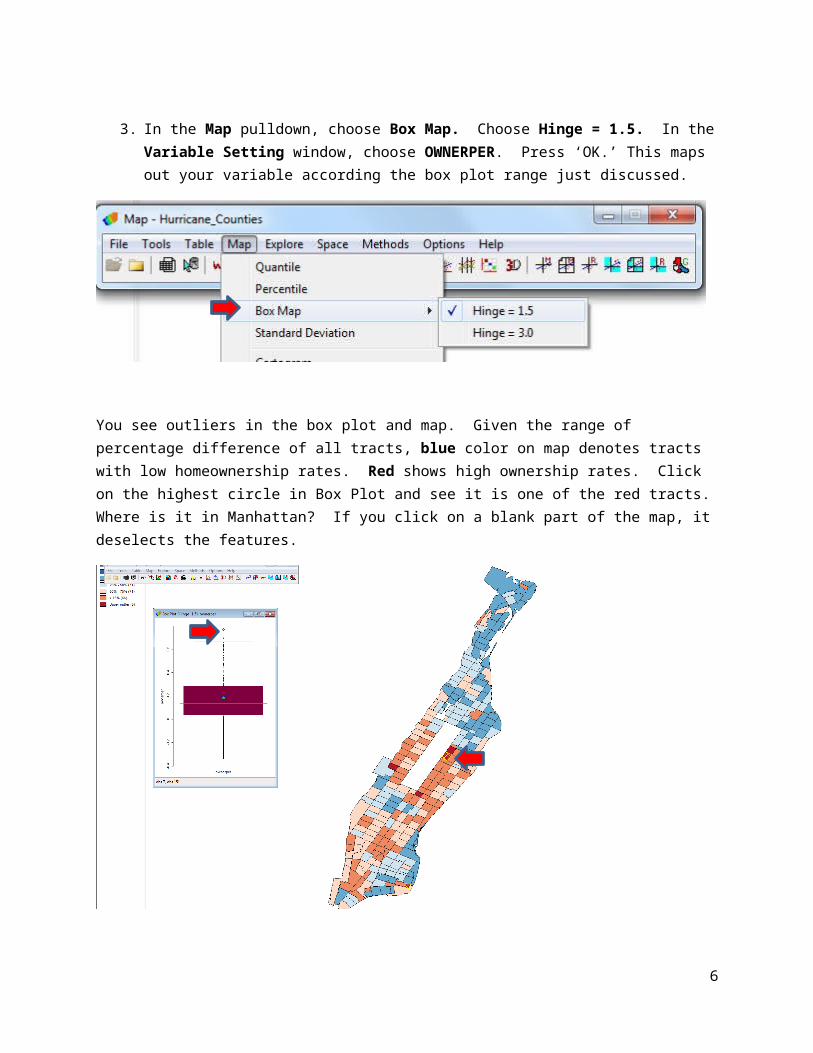
3. In the Map pulldown, choose Box Map. Choose Hinge = 1.5. In the Variable Setting window, choose OWNERPER. Press ‘OK.’ This maps out your variable according the box plot range just discussed.

You see outliers in the box plot and map. Given the range of percentage difference of all tracts, blue color on map denotes tracts with low homeownership rates. Red shows high ownership rates. Click on the highest circle in Box Plot and see it is one of the red tracts. Where is it in Manhattan? If you click on a blank part of the map, it deselects the features.

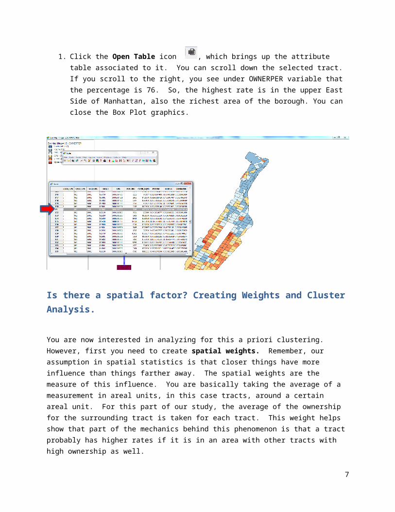
1. Click the Open Table icon , which brings up the attribute table associated to it. You can scroll down the selected tract. If you scroll to the right, you see under OWNERPER variable that

5

the percentage is 76. So, the highest rate is in the upper East Side of Manhattan, also the richest area of the borough. You can close the Box Plot graphics.

Is there a spatial factor? Creating Weights and Cluster Analysis.

You are now interested in analyzing for this a priori clustering. However, first you need to create spatial weights. Remember, our assumption in spatial statistics is that closer things have more influence than things farther away. The spatial weights are the measure of this influence. You are basically taking the average of a measurement in areal units, in this case tracts, around a certain areal unit. For this part of our study, the average of the ownership for the surrounding tract is taken for each tract. This weight helps show that part of the mechanics behind this phenomenon is that a tract probably has higher rates if it is in an area with other tracts with high ownership as well.

You have many options for creating spatial weights. You can use distance to make weights (e.g. < 60 miles), K neighbors (e.g. only 4 near neighbors) and socio-economic factors (e.g. employment rates). For more discussion on these kinds of weights, please see the presentations under Spatial Weights (https://geodacenter.asu.edu/eslides). In this case, you are interested in contiguity. You want to see if tracts are indeed next to and clustering with other tracts according to ownership. Let’s create the weights.

1. In the Tools menu, select Weights. In the next pop-up menu, choose Create.

6

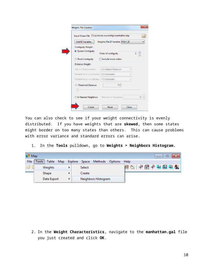
2. In the Weights File Creation window, you first need a unique number for each tract. Click Add ID Variable. In the new Add new ID Variable window, a new POLY_ID variable is suggested in the Enter new ID variable name: field. This new variable is populated with unique numbers for each tract. Accept it. Click Save to DBF File. When prompted in a new window to accept new variable, click YES and then OK when told in a new window that it has been added successfully.

3. In the Contiguity Weight, you now decide between Queen or Rook Contiguities. Think of a chess board. Rook Contiguity means the tracts share common boundaries that are similar to a Rook movement. Queen Contiguity is like the movement of a Queen (common boundaries and vertices).

Rook Queen

Tract Tract

7

Let theory drive your decision in choosing between which one. Is there reason to think that there is flow or influence going across all corners of the units of analysis? In this instance, you can choose Queen and then click Create at the bottom. When prompted, navigate to your storage device and save the weights file with the .gal extension. Close out of the Message and Weights File Creation windows when done.

You can also check to see if your weight connectivity is evenly distributed. If you have weights that are skewed, then some states might border on too many states than others. This can cause problems with error variance and standard errors can arise.

1. In the Tools pulldown, go to Weights > Neighbors Histogram.

8

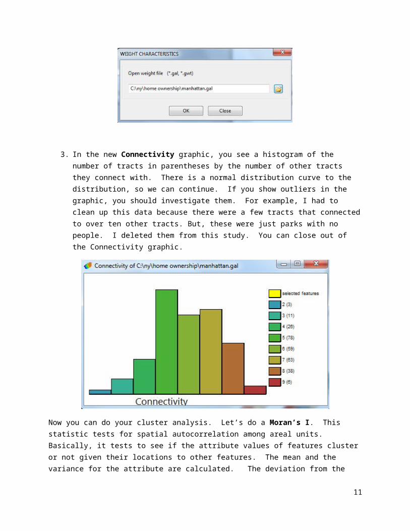
2. In the Weight Characteristics, navigate to the manhattan.gal file you just created and click OK.

3. In the new Connectivity graphic, you see a histogram of the number of tracts in parentheses by the number of other tracts they connect with. There is a normal distribution curve to the distribution, so we can continue. If you show outliers in the graphic, you should investigate them. For example, I had to clean up this data because there were a few tracts that connected to over ten other tracts. But, these were just parks with no people. I deleted them from this study. You can close out of the Connectivity graphic.

Now you can do your cluster analysis. Let’s do a Moran’s I. This statistic tests for spatial autocorrelation among areal units. Basically, it tests to see if the attribute values of features cluster or not given their locations to other features. The mean and the variance for the attribute are calculated. The deviation from the mean for each feature is then multiplied with neighboring features to create a cross-product. If many neighboring features have high or low cross-products, then there is clustering.

The test result is interpreted like a correlation result. This gives you a global result for the entire research area.

9

For information regarding the Moran’s I equation, please consult http://en.wikipedia.org/wiki/Moran%27s_I

1. Click on Univariate Moran to start the function.

10

A result of - 1 would give you a checkered pattern

A result of 0 would give you a random pattern

A result of 1 would give you a clustered pattern

2. In Variable Settings, choose the variable that you want to test. Select OWNERPER in menu. Click OK.

3. If prompted, in Select Weight, you must select the weight that you set up for your analysis. To do so, in Select from file (gal, gwt), navigate to the manhattan.gal. Click OK.

11

In the Moran Scatter Plot window, you get your test result, which is Moran’s I = .491. This shows a moderate/high autocorrelation in your research area. But, is it significant?

1. Right-click on the Moran Scatter Plot and in the pop up menu, select Randomization. Now choose how many permutations or running of the model to give you your test parameters. Choose 999 Permutations.

12

In the Randomization window, use the pseudo p-value for reporting the p value in your results. In this instance, p = .001, so it’s definitely significant.

Close the Randomization and Scatter Plot windows.

Moran’s I gives you a global statistic. So, you know there is clustering going on in the research area, but we don’t know exactly where or how. To investigate further, you can do a Local Indicators of Spatial Association (LISA). This test not only tests for regional clustering, it can also show the presence of significant spatial clusters or outliers by state.

1. Click on univariate LISA

13

2. In Variable Setting, scroll to OWNERPER in the menu. Click OK.

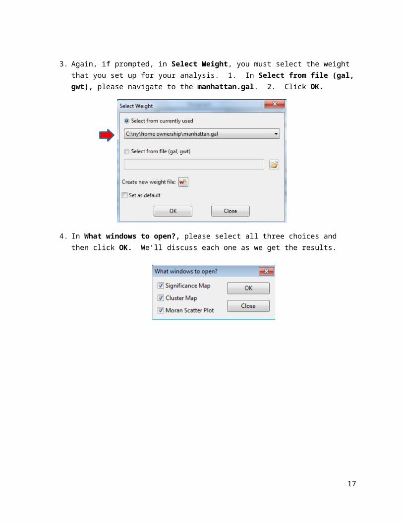
3. Again, if prompted, in Select Weight, you must select the weight that you set up for your analysis. 1. In Select from file (gal, gwt), please navigate to the manhattan.gal. 2. Click OK.

4. In What windows to open?, please select all three choices and then click OK. We’ll discuss each one as we get the results.

14

15

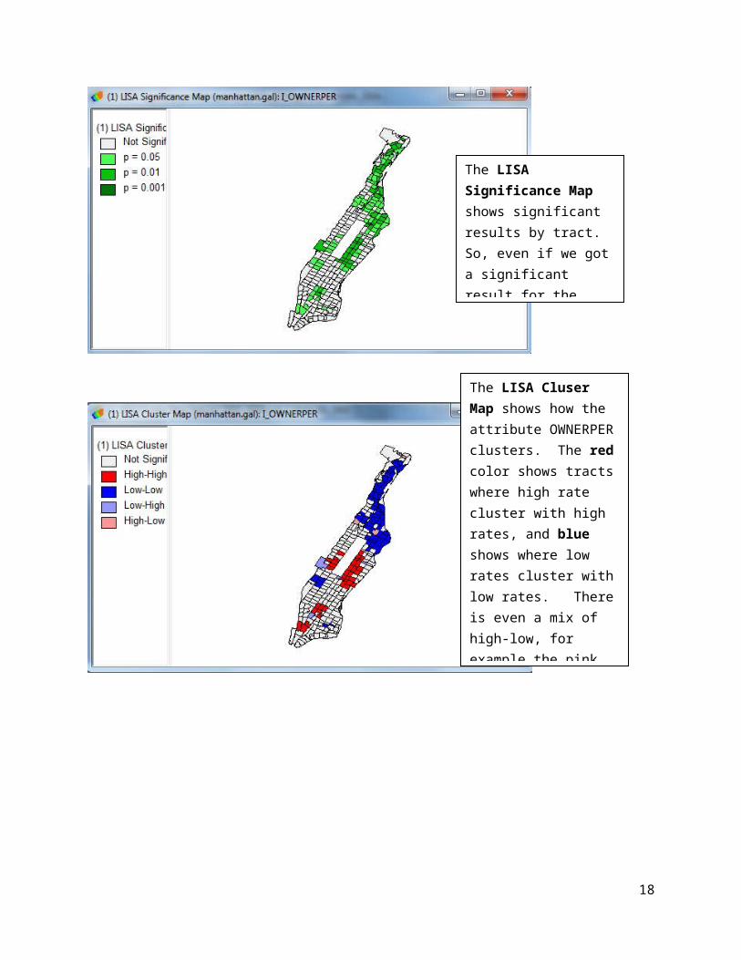
The LISA Significance Map shows significant results by tract. So, even if we got a significant result for the whole research area, only some tracts really show significant clustering.

The LISA Cluser Map shows how the attribute OWNERPER clusters. The red color shows tracts where high rate cluster with high rates, and blue shows where low rates cluster with low rates. There is even a mix of high-low, for example the pink color. So, there is a cluster of high ownership midtown and clusters of lower ownership uptown.

From the LISA, we can ascertain that there was statistically significant moderate clustering in Manhattan. Lower home ownership seems to cluster in poorer, non-white areas.

Reporting Results: Report at least the Moran’s I test value and the p value. So, for this test, you should report Moran’s I = .491, p = .001. Including the LISA cluster map is also a great way of showing how the attribute is actually clustering.

You can close out of all the results windows, but not Map – OWNERPER.

Incorporating spatial dependency: Spatial Regression

Regression (http://en.wikipedia.org/wiki/Regression_analysis) is ability to predict a value of an outcome (dependent) variable based on values of explanatory (independent) variables. Based on correlation, linear regression investigates whether an increase in the units of measurement of the independent variables increases or decreases the units of measurement of the dependent variable. In this case, you want to discern how much of the home ownership attribute (dependent) can be explained by social variables (independent). In the social sciences, these kinds of model building are used to help explain why the phenomenon happened. We know already that there is spatial dependency from our Moran’s I, so this also needs to be built into the model.

16

A Moran Scatter Plot is produced again. The LISA function is additionally very useful because it can create the global statistics in graphic form along with the local statistics.

First, when choosing independent variables for a regression model, you want to select something that theoretically makes sense. In this model, you want to explain why more people own their homes than others. Social and economic reasons seem reasonable in clarifying this. We have chosen three variables for possible explanatory variables: percentage of foreign born population (FORPOR), percentage of people under the poverty line (POVPER), and population per square mile (POP00_SQMI). We first will do a normal OLS Regression that does not use spatial weights.

1. In the Methods pulldown, choose Regression. 2. In the Regression Title and Output window, you can change the name of the results Report Title

if desired. We will just leave the name Regression. If you want, in Information in the output includes, you can include generate residuals, predicated values, etc. Click OK.

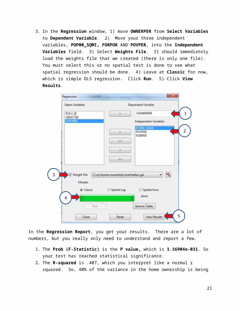
3. In the Regression window, 1) move OWNERPER from Select Variables to Dependent Variable. 2) Move your three independent variables, POP00_SQMI, FORPOR AND POVPER, into the Independent Variables field. 3) Select Weights File. It should immediately load the weights file that we created (there is only one file). You must select this or no spatial test is done to see what spatial regression should be done. 4) Leave at Classic for now, which is simple OLS regression. Click Run. 5) Click View Results.

17

In the Regression Report, you get your results. There are a lot of numbers, but you really only need to understand and report a few.

1. The Prob (F-Statistic) is the P value, which is 1.16904e-031. So your test has reached statistical significance.

2. The R-squared is .407, which you interpret like a normal r squared. So, 40% of the variance in the home ownership is being explained by our three independent variables. This model is moderately effective.

3. The Akaike info criterion and Schwarz criterion are important for spatial regression. They report on the goodness of fit for the models (http://en.wikipedia.org/wiki/Akaike_information_criterion). The lower this value is, the more accurate the test is.

4. Look at the independent variables. Under Probability, two of the independent variables, POVPER and FORPER, are significant, > 0.000 and .0003 respectively. POP00_SQMI is not at .782.

5. Under Coefficient, you see how strong each variable is in the model. You multiply the coefficient by the slope to get the unit change. So, POVPER is -0.684. So if you increase the poverty rate by one percent, you decrease the home ownership by -0.684 (1 (increase in poverty rate) * -0.684 (poverty coefficient) = -0.684 percent increase in home ownership).

18

2

1

3

4

5

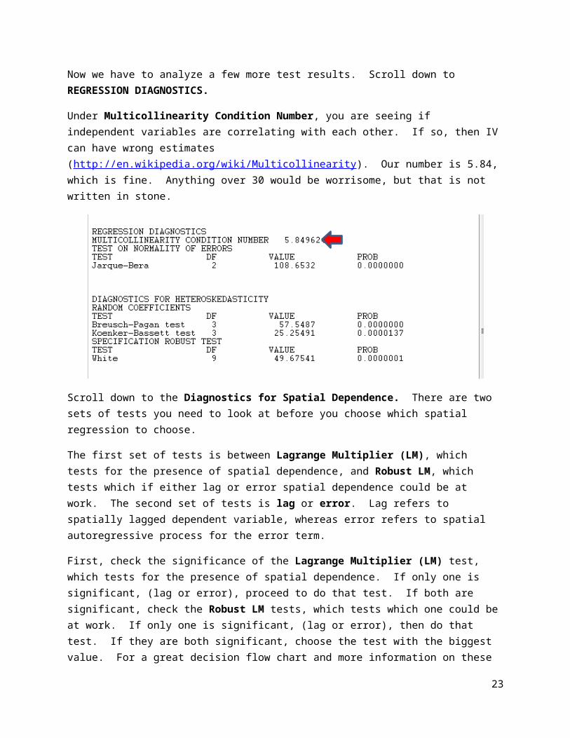
Now we have to analyze a few more test results. Scroll down to REGRESSION DIAGNOSTICS.

Under Multicollinearity Condition Number, you are seeing if independent variables are correlating with each other. If so, then IV can have wrong estimates (http://en.wikipedia.org/wiki/Multicollinearity). Our number is 5.84, which is fine. Anything over 30 would be worrisome, but that is not written in stone.

19

12

3

45

Scroll down to the Diagnostics for Spatial Dependence. There are two sets of tests you need to look at before you choose which spatial regression to choose.

The first set of tests is between Lagrange Multiplier (LM), which tests for the presence of spatial dependence, and Robust LM, which tests which if either lag or error spatial dependence could be at work. The second set of tests is lag or error. Lag refers to spatially lagged dependent variable, whereas error refers to spatial autoregressive process for the error term.

First, check the significance of the Lagrange Multiplier (LM) test, which tests for the presence of spatial dependence. If only one is significant, (lag or error), proceed to do that test. If both are significant, check the Robust LM tests, which tests which one could be at work. If only one is significant, (lag or error), then do that test. If they are both significant, choose the test with the biggest value. For a great decision flow chart and more information on these tests, look at Luc Anselin’s Exploring Spatial Data with Geoda on pg. 198 at (https://geodacenter.asu.edu/system/files/geodaworkbook.pdf)

Let’s look at our results. 1) First, we’ll check the Lagrange Multiplier for Lag and Error. Both are significant at p > .001. 2) Since both LM were significant, now check the Robust LM (lag) and (error). Both are significant at p = .030 and p = .028 respectively. So, choose the one with the biggest test value, which would be Robust LM (error) at 4.777. You can close the Results

20

4. Back in the Regression window, 1) under Models choose Spatial Error, 2) click Run, then 3) View Results.

.

21

1

3

2

In the Regression Report, scroll down to Summary of Output: Spatial Error Model. 1) One way of understanding the results in to compare the R-squared. This went up to .530. So, now it’s a stronger model. 2) What is very important are the Akaike info criterion and Schwarz criterion. You must make sure that these numbers went down in order to ensure that this test is more accurate than the OLS. In OLS regression, Akaike info criterion was -335, and now it’s -383, and the Schwarz criterion was -321, and now it’s -368. So the numbers went down suggesting that this is better test. 3) You need to also report your IVs. They are reasonably the same as the OLS. Pop00_SQMI is still insignificant, and POVPER and FORPER are still significant with about the same coefficients. Our take home message for this test is that for home ownership in Manhattan, space matters. When the spatial weights are taken into consideration in the model (Spatial Lag Model), the spatial regression becomes noticeably stronger in predicting the DV than a simple OLS Regression. The two IV of FORPER and POVPER are significant predictors for home ownership in this test area.

Using a chart is a great way to report your results. One way or reporting is to compare the OLS and ERROR regression models:

Coefficients OLS ERRORPOP00_SQMI 4.511867e-008 3.11906e-008 POVPER -0.684 -0.583*FORPER -0.393 -0.402*R-Squared 0.407 0.530Akaike info criterion -335.83 -383.311Schwarz orientation -321.23 -368.715*Significance at p < .001

22

2

3

1

Further work:

1. Investigate the murder rate in the south using the variable HC90 (Average of Number of Homicides for 1989-91) in S:\Tutorials\Tufts\Tutorial Data\Spatial Statistics\south.

a. What weights did you use?b. Please report the Moran’s I? Interpret your results. c. Please show the Moran’s map.

2. Now, using the same dataset, use HC90 as your DV. Your IV are RD90 Resource Deprivation/Affluence Component (prinicipal component composed of percent black, log of median family income, gini index of family income inequality, percent of families, female headed), PS90 Population Structure Component (prinicipal component composed of the log of population and the log of population density), DV90 (Percent of males 15 and over who are divorces) and UE90 (Percent of civilian labor force that is unemployed).

a. What spatial model is better, Error or lag?b. Please report your results below.

Coefficients OLS ERRORPOP00_SQMI POVPERFORPERR-SquaredAkaike info criterionSchwarz orientation

Note: We did not cover the heteroskedescity tests (http://en.wikipedia.org/wiki/Heteroscedasticity) in this tutorial. You can follow up at https://geodacenter.asu.edu/system/files/geodaworkbook.pdf.

23