Spatial Smoothing and Broadband Beamforming

Bhaskar D RaoUniversity of California, San Diego

Email: brao@ucsd.edu

Reference Books and Papers

1. Optimum Array Processing, H. L. Van Trees

2. Stoica, P., & Moses, R. L. (2005). Spectral analysis of signals (Vol.1). Upper Saddle River, NJ: Pearson Prentice Hall.

3. Schmidt, R. (1986). Multiple emitter location and signal parameterestimation. IEEE transactions on antennas and propagation, 34(3),276-280.

4. Roy, Richard, and Thomas Kailath. ”ESPRIT-estimation of signalparameters via rotational invariance techniques.” IEEE Transactionson acoustics, speech, and signal processing 37.7 (1989): 984-995.

5. Rao, Bhaskar D., and K. S. Arun. ”Model based processing ofsignals: A state space approach.” Proceedings of the IEEE 80.2(1992): 283-309.

Narrow-band Signals

x(ωc , n) = V(ωc , ks)Fs [n] +D−1∑l=1

V(ωc , kl)Fl [n] + Z[n]

Assumptions

I Fs [n], Fl [n], l = 1, ..,D − 1, and Z[n] are zero mean

I E (|Fs [n]|2) = ps , and E (|Fl [n]|2 = pl , l = 1, . . . ,D − 1, andE (Z[n]ZH [n]) = σ2

z I

I All the signals/sources are uncorrelated with each other and overtime: E (Fl [n]F ∗m[p]) = plδ[l −m]δ[n − p] and E (Fl [n]F ∗s [p]) = 0

I The sources are uncorrelated with the noise: E (Z[n]F ∗l [m]) = 0

Direction of Arrival (DOA) Estimation

x[n] =D−1∑l=0

VlFl [n] + Z[n], n = 0, 1, . . . , L− 1

Here we have chosen to denote Vs by V0 for simplicity of notation. NoteVl = V(kl). We will refer to the L vector measurements as L snapshots.

Goal: Estimate the direction of arrival kl or equivalently(θl , φl), l = 0, ...,D − 1.Can also consider estimating the source powers pl , l = 0, 1, ...,D − 1, andnoise variance σ2

z .

ULA :V(ψ) = [e−j

N−12 ψ, . . . , e j

N−12 ψ]T = e−j

N−12 ψ[1, e jψ, e j2ψ, ..., e j(N−1)ψ]T

Note for a ULA, V(ψ) = JV∗(ψ), where J is all zeros except for onesalong the anti-diagonal. Also note J2 = I.

ULA and Time Series

ULAx0[n]x1[n]

...xN−1[n]

=D−1∑l=0

1

e jψl

...e j(N−1)ψl

e−jN−1

2 ψlFl [n]+Z[n], n = 0, 1, . . . , L−1

Similar to a time series problems composed of complex exponentialsx [n] =

∑D−1l=0 cle

jωln + z [n], n = 0, 1, . . . , (M − 1).In vector form, the time series measurement is

x [0]x [1]

...x [M − 1]

=D−1∑l=0

1

e jωl

...e j(M−1)ωl

cl +

z [0]z [1]

...z [M − 1]

The sum of exponentials problem with M samples is equivalent to a ULAwith M sensors and one (vector) measurement or one snapshotIn array processing we have a limited number of sensors N but cancompensate potentially with L snapshots.The time series problem is equivalent to one snapshot but a potentiallylarge array if the number of samples M is large.

Observations

Sx = Ss + σ2z I

= Es (Λs + σ2z ID×D) EH

s + σ2zEnE

Hn

=D∑l=1

(λsl + σ2z )qlq

Hl + σ2

z

N∑l=(D+1)

qlqHl

I Sx has eigenvalues λl = λsl + σ2z , l = 1, . . . ,D, and

λl = σ2z , l = (D + 1), . . . ,N

I The number of sources D can be identified by examining themultiplicity of the smallest eigenvalue which is expected to be σ2

z

with multiplicity (N − D)

I The eigenvectors corresponding to the signal subspaces and noisesubspaces are readily available from the eigen decomposition of Sx ,i.e. Es and En are easily extracted.

MUltiple SIgnal Classification (MUSIC)

MUSIC uses the noise subspace spanned by the ”noise” eigenvectors En.

Since R(V) = R(Es) ⊥ R(En), we haveVl ⊥ R(En), l = 0, 1, . . . , (D − 1) or VH

l En = 0, l = 0, 1, . . . , (D − 1)Many options to use this orthogonality property. All methods start withSx , usually estimated from the data.

MUSIC Algorithm (also known as Spectral-MUSIC)

I Perform an eigen-decomposition of Sx

I Estimate D and the signal subspace Es and the noise subspace En

I Compute the spatial MUSIC spectrum as follows:

PMUSIC (k) =1

|VH(k)En|2

Note that |VH(k)En|2 = VH(k)EnEHn V(k) = VH(k)PnV(k) where

Pn = EnEHn

I The peaks in PMUSIC (k) gives us the DOA.

Root-MUSIC Algorithm for ULAs

I Perform an eigen-decomposition of Sx

I Estimate D and the signal subspace Es and the noise subspace En

I Compute ql(z) =∑N−1

m=0 ql [m]z−m, l = D + 1, . . . ,N − 1.

I Compute B(z) =∑N

l=D+1 Bl(z) where

Bl(z) = ql(z)q∗l ( 1z∗ ) =

∑N−1l=−(N−1) rql [m]z−m

I Perform a spectral factorization to find a minimum phase factorHrm(z), i.e. B(z) = Hrm(z)H∗rm( 1

z∗ ).

I The D roots on/close to the unit circle are identified and theirargument used to estimate the DOA

ESPRIT algorithm

I Perform an eigen-decomposition of Sx

I Estimate D and the signal subspace Es and the noise subspace En

I From Es determine E1 as the first (N − 1) rows and E2 as the last(N − 1) rows of Es

I Compute Φ by solving E2 = E1Φ using a Least Squares Approach,i.e. Φ = E+

1 E2.

I Perform an eigen-decomposition of Φ

I The argument of the D eigenvalues are used to estimate the DOA

As in the minimum norm method, E+1 can be obtained efficiently using

the matrix inversion lemma and the computation of Φ can be simplified.Another option is to use a Total Least Squares approach, as opposed to aLeast Squares approach, to estimate Φ

ESPRIT: ULA and Doublets

ESPRIT with Doublets: Theory

If the array manifold for the first array is v1(k), and the array manifoldfor the second array is v2(k),then for a plane with wavenumber kl , wehave v2(kl) = v1(kl)e−jωcτl . The overall array manifold has the form

V(kl) =

[v1(kl)v2(kl)

]=

[v1(kl)

v1(kl)e−jωcτl

]Now consider D plane waves. The signal subspace

V = [V0,V1, . . . ,VD−1] =

[v1(k0) v1(k1) . . . v1(kD−1)v2(k0) v2(k1) . . . v2(kD−1)

]=

[V1

V2

]=

[v1(k0) v1(k1) . . . v1(kD−1)

v1(kl)e−jωcτ0 v1(kl)e−jωcτ1 . . . v1(kl)e−jωcτD−1

]=

[V1

V1Ψ

]An ESPRIT algorithm can be developed now with

Es =

[E1

E2

]with E2 = E1Φ

Coherent Sources

Sx = Ss + σ2z I = VSFV

H + σ2z I

The dimension D of the signal subspace depends on the rank of thesource covariance matrix SF .

If the sources are highly correlated, SF can be ill-conditioned or singular.This can make the dimension of the signal subspace less than D and inparticular when an estimate of Sx is used.

Spatial Smoothing for ULAs: A technique to overcome this rankdeficiency problem.

Spatial Smoothing

We will consider the ULA as two sub-arrays as in ESPRIT: subarray 1 isthe first (N − 1) sensors and subarray 2 is the last (N − 1) sensors.Since the data is given by x[n] = VF[n] + Z[n], we have the data fromthe two sub-arrays given by

x1[n] = V1F[n] + Z1[n] and x2[n] = V2F[n] + Z2[n]

Covariance of the two subarrays are given by

S(1)x = V1SFV

H1 + σ2

z I and S(2)x = V2SFV

H2 + σ2

z I = V1ΨSFΨHVH1 + σ2

z I

Spatially Smoothed Covariance

S(s)x =

1

2

(S(1)x + S(2)

x

)=

1

2

(V1SFV

H1 + σ2

z I + V2SFVH2 + σ2

z I)

=1

2

(V1SFV

H1 + V1ΨSFΨHVH

1

)+ σ2

z I

= V1

(SF + ΨSFΨH

2

)VH

1 = V1SFVH1

SF = SF +ΨSF ΨH

2 is more likely to have rank D restoring the signalsubspace dimension in the spatially smoothed covariance matrix

Spatial Smoothing Cont’d

We can generalize this idea by viewing the ULA as P sub-arrays: subarray1 is the first (N − P + 1) sensors, and subarray 2 is the next (N − P + 1)sensors and so on.Since the data is given by x[n] = VF[n] + Z[n], we have the data fromthe l sub-array given by

xl [n] = VlF[n] + Zl [n], l = 1, 2, ..,P with Vl = V1Ψl−1

Covariance of the lth sub-array is given by

S(l)x = VlSFV

Hl + σ2

z I = V1Ψl−1S(ΨH)l−1V1 + σ2z I

Spatially Smoothed Covariance

S(s)x =

1

P

P∑l=1

S(l)x = V1SFV

H1

SF = 1P

∑Pl=1 Ψl−1SF (ΨH)l−1 is more likely to have rank D restoring the

signal subspace dimension in the spatially smoothed covariance matrix

Covariance Estimation

Given L snapshots

Sx =1

L

L−1∑n=0

x[n]xH [n] =1

LDDH , where D = [x[0], x[1], . . . , x[L− 1]]

Smoothed Covariance Estimate

S(s)x =

1

P

P∑l=1

S(l)x =

1

PL

P∑l=1

DlDHl where Dl = [xl [0], xl [1], . . . , xl [L− 1]]

and xl [n] = [xl−1[n], xl [n], . . . , xN−P+l−1[n]]T .For P = 2, we have x1[n] = [x0[n], x1[n], . . . , xN−2[n]]T andx2[n] = [x1[n], x2[n], . . . , xN−l [n]]T .Alternatively, we can express the smoothed covariance estimate as

S(s)x =

1

L

L−1∑n=0

Ds [n]DHs [n], where Ds [n] = [x1[n], x2[n], . . . , xP [n]]

Time Series: Sum of Exponentials

x [n], n = 0, 1, . . . ,M − 1: L = 1, one snapshot, array size N = M, whereM is the number of samples containing D exponentials.To compute a covariance matrix, we have to do smoothing.

Ds =

x [0] x [1] . . . x [P − 1]x [1] x [2] . . . x [P]

......

......

x [M − P] x [M − P + 1] . . . x [M − 1]

The smoothed covariance can be computed a S

(s)x = 1

PDsDHs .

Since we need rank of the matrix to be greater than D, we need P > Dand M − P + 1 > D. This requires M > 2D.

Instead of an eigen-decomposition of S(s)x , one can do a SVD of Ds .

Numerically superior.Can use MUSIC, ESPRIT or any subspace method to estimate thefrequencies ωl .

Forward-Backward (FB) Smoothing for ULAs

For a ULA, we have JV∗(ψ) = V(ψ). Hence

JS∗xJ = JV∗S∗FVTJ + σ2

zJIJ = VS∗FVH + σ2

z I

The signal subspace of JS∗xJ is also spanned by V and so subspacemethods MUSIC etc can be applied to JS∗xJ.The FB covariance estimate

SFBx =

1

2(Sx + JS∗xJ) =

1

2V(SF + S∗F )VH + σ2

z I

Subspace methods can be readily applied to estimated SFBx . The FB

covariance matrix has a better condition number and so improvesperformance.The FB approach can be applied to spatial smoothing, i.e.12

(S

(s)x + JS

∗(s)x J

)and also to the time series [Ds , JD∗s ].

Broadband Signals

Narrow band signals: f (t− τ)e jωc (t−τ) ≈ f (t)e jωc (t−τ), for τ << T = 12B

The signal becomes broadband if the bandwidth becomes large and thedelay across the array can no longer be considered small compared to thesampling interval

Signals such as speech signals are naturally baseband signals and arebroadband in nature

Delay and Sum beamformer

Delay the output of the sensors appropriately and enable constructiveaddition of the copies to get SNR improvement over white noiseIn the presence of an interferer will use FIR filters at the output to cancelor suppress interference

Time-Delay Estimation: Preliminaries1

rx1x2 [m] = E (x1[n + m]x∗2 [n]) and from LTI systems theory we know thecross-power spectrum is given by

Sy1y2 (e jω) =∞∑

m=−∞ry1y2 [m]e−jωm = H1(e jω)H∗2 (e jω)Sx1x2 (e jω)

Sy1y1 (e jω) is the power spectrum which is real and positive.If we are given data, we can divide the data into L blocks of length Nand estimate the cross-power spectrum using the FFT

1Carter, G. Clifford. Coherence and time delay estimation: an appliedtutorial for research, development, test, and evaluation engineers. IEEE, 1993.

Time Delay Estimation

y1[n] = r1(nT ) = s[n] + z1[n]

y2[n] = r2(nT ) = s[n − D] + z2[n]

Assuming the noises are uncorrelated, ry2y1 [m] = rss [m − D].

D = arg maxm

ry2y1 [m] = arg maxm

1

2π

∫ π

−πSy2y1 (e jω)e jωmdω

The peak is sharp if s[n] is a white noise sequence and in the absence ofreverberation/multipath.

Generalized Cross-Correlation (GCC) Methods

D = arg maxm

1

2π

∫ π

−πφ(e jω)Sy2y1 (e jω)e jωmdω

Cross-Correlation Method: φ(e jω) = 1The purpose of φ(e jω) is to whiten the signal and/or weight thespectrum based on the SNR in the frequency domain. Note thatSy2y1 (e jω) = Sss(e jω)e−jωD .PHAse Transform (PHAT): φ(e jω) = 1

|Sy2y1(e jω)|

Smoothed COherence Transform (SCOT): φ(e jω) = 1√Sy1y1

(e jω)Sy2y2(e jω)

Maximum-Likelihood (ML): φ(e jω) = 1|Sy2y1

(e jω)||γy2y1

(e jω)|2

1−|γy2y1(e jω)|2 where

γy2y1 (e jω) =Sy2y1 (e jω)√

Sy1y1 (e jω)Sy2y2 (e jω), 0 ≤ |γy2y1 (e jω)| ≤ 1,∀ω

is the coherence function.

Adaptive Broadband Beamformer2

2Frost, Otis Lamont. ”An algorithm for linearly constrained adaptive arrayprocessing.” Proceedings of the IEEE 60.8 (1972): 926-935.

Wideband BF Formulation

Number of sensors: N = K , number of taps, i.e. order of FIR filters is J.

If we denote the input measurement vector as x[n], then the data in thetap delay line is [x[n], x[n − 1], . . . , x[n − J + 1]]

Weights: Using vector notation, the weights in the tap delay line are[W0,W1, . . . ,WJ−1] , where Wk = [wk,0,wk,1, . . . ,wk,N−1].

Key Question: How to characterize and design such an array?

Characterization: Frequency-Wavenumber Response

Extension of the MPDR formulation: Look direction constraint plusminimize output power

Frequency Wavenumber Response

If the source signal is s(t) = e jΩt from direction k, then the signalreceived at sensor l is delayed relative to the origin by τl .

xl(t) = s(t) = e jΩ(t−τl ) or xl [n] = xl(nT ) = e jΩ(nT−τl ) = e jω(n−τl )

where ω = ΩT and τl = 1T τl .

xl [n]→ Hl(z)→ yl [n] = e jω(n−τl )Hl(ejω)

The array output

y [n] =N−1∑l=0

yl [n] =N−1∑l=0

e jω(n−τl )Hl(ejω) = e jωn

N−1∑l=0

e jωτlHl(ejω) = e jωnB(ω, k)

B(ω, k) =∑N−1

l=0 e jωτlHl(ejω) is the frequency-wavenumber response of

array

Time-Domain Formulation

Beamformer output

y [n] = W T0 x[n] +W T

1 x[n−1] + . . .+W TJ−1x[n−J + 1] =

J−1∑k=0

W Tk x[n−k]

Constraints: Define 1 = [1, 1, . . . , 1]T , a vector in RN .

N−1∑m=0

wk,m = fk or 1TWk = fk , k = 0, 1, . . . , J − 1

This is equivalent to look direction transfer function constraint of

Hd(z) = F (z) = f0 + f1z−1 + . . .+ fJ−1z

−(J−1) =J−1∑m=0

fmz−m

Frost Beamformer

Stacking all the BF weights and the constraints into large vectors ofdimension NJ, we have

y [n] = WTX[n], where W = [W T0 ,W

T1 , . . . ,W

TJ−1]T

and X[n] = [xT [n], xT [n − 1], . . . , xT [n − J + 1]]T .The output power is E (y2[n]) = WTRxxW where Rxx = E (X[n]XT [n]).The constraints are given by

CTW = f or

1T 0 . . . 00 1T . . . 0...

......

...0 0 . . . 1T

W =

f1f2...

fJ−1

The optimization problem is

minW

WTRxxW subject to CTW = f

Using Lagrange multipliers, we can show

Wo = R−1xx C(CTR−1

xx C)−1f

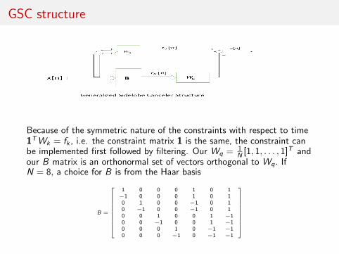
GSC structure

Because of the symmetric nature of the constraints with respect to time1TWk = fk , i.e. the constraint matrix 1 is the same, the constraint canbe implemented first followed by filtering. Our Wq = 1

N [1, 1, . . . , 1]T andour B matrix is an orthonormal set of vectors orthogonal to Wq. IfN = 8, a choice for B is from the Haar basis

B =

1 0 0 0 1 0 1−1 0 0 0 1 0 10 1 0 0 −1 0 10 −1 0 0 −1 0 10 0 1 0 0 1 −10 0 −1 0 0 1 −10 0 0 1 0 −1 −10 0 0 −1 0 −1 −1

GSC Implementation of Adaptive Broadband BF3

3Griffiths, Lloyd, and C. W. Jim. ”An alternative approach to linearlyconstrained adaptive beamforming.” IEEE Transactions on antennas andpropagation 30.1 (1982): 27-34.