spatial mapping of agricultural water productivity...

IRRIGATION AND DRAINAGE

Irrig. and Drain. 61: 60–79 (2012)

Published online 15 March 2011 in Wiley Online Library (wileyonlinelibrary.com) DOI: 10.1002/ird.618

SPATIAL MAPPING OF AGRICULTURAL WATER PRODUCTIVITY USING THE SWATMODEL IN UPPER BHIMA CATCHMENT, INDIA†

KAUSHAL K. GARG1*, LUNA BHARATI2, ANJU GAUR3, BIJU GEORGE4, SREEDHAR ACHARYA5,KIRAN JELLA5 AND B. NARASIMHAN6

1International Crops Research Institute for the Semi‐Arid Tropics, Patancheru, India2International Water Management Institute‐Nepal, Jawalakhel, Lalitpur, Nepal

3The World Bank, New Delhi, India4Department of Civil and Environmental Engineering, University of Melbourne, Australia

5International Water Management Institute‐Patancheru, Patancheru, India6Indian Institute of Technology, Chennai, India

ABSTRACT

The Upper Bhima River Basin is facing both episodic and chronic water shortages due to intensive irrigation development. Themain objective of this study was to characterize the hydrologic processes of the Upper Bhima River Basin and assess crop waterproductivity using the distributed hydrologic model, SWAT. Rainfall within the basin varies from 450 to 5000mm in a period of3–4months. The basin has an average rainfall of 711mm (32 400Mm3 (million cubic metres)) in a normal year, of which 12.8%(4150Mm3) and 21% (6800Mm3) are captured by the reservoirs and groundwater reserves, respectively, 7% (2260Mm3)exported as runoff out of the basin and the rest (63%) used in evapotranspiration. Agricultural water productivity for sugarcane,sorghum and millet were estimated as 2.90, 0.51 and 0.30 kg m¯3, respectively, which were significantly lower than the potentialand global maximum in the basin and warrant further improvement. Various scenarios involving different cropping patterns weretested with the goal of increasing economic water productivity values in the Ujjani Irrigation Scheme. Analysis suggests thatmaximization of the area by provision of supplemental irrigation to rainfed areas as well as better on‐farm water managementpractices can provide opportunities for improving water productivity. Copyright © 2011 John Wiley & Sons, Ltd.

key words: hydrological modelling; SWAT; crop water productivity; water balance; Upper Bhima; Ujjani Irrigation Scheme

Received 16 March 2010; Revised 3 December 2010; Accepted 3 December 2010

RÉSUMÉ

Le bassin versant du Haut‐Bhima est confronté aux pénuries d’eau épisodiques et chroniques à cause de développement del’irrigation intensive. L’objectif principal de cette étude est de caractériser les processus hydrologiques de ce bassin versant duHaut‐Bhima et d’évaluer la productivité en eau des cultures en utilisant SWAT, le modèle hydrologique distribué. Lesprécipitations dans le bassin versant varient de 450mm/an à 5000mm/an et sont réparties inégalement dans le temps et dansl’espace. Le bassin a une pluviométrie moyenne de 711mm (32 400Mm3) dans une année normale, dont 12.8% (4150Mm3)et 21% (6800Mm3) remplissent ou rechargent les réservoirs ou les nappes phréatiques, 7% (2260Mm3) ruissellent, et le reste(63%) est prélevé pour l’évapotranspiration. La productivité de l’eau agricole dans le bassin pour la canne à sucre, le sorgho et lemil ont été estimés à 2.90, 0.51 et 0.30 kg m¯3, ce qui est significativement plus faible que le potentiel maximal habituellementrencontré dans le monde. Il y a donc des marges de progrès qu’il convient d’explorer. Différents scénarios impliquant différentsitinéraires techniques ont été testés dans le but d’accroître la valeur économique de la productivité de l’eau dans le systèmed’irrigation d’Ujjani. L’analyse suggère que la maximisation de la superficie grâce à la fourniture d’irrigation d’appoint pour leszones pluviales, ainsi que le recours à des pratiques agricoles de gestion plus économes en eau, peuvent offrir des possibilités pouraméliorer la productivité de l’eau. Copyright © 2011 John Wiley & Sons, Ltd.

mots clés: modélisation hydrologique; SWAT; productivité en eau des cultures; gestion équilibrée de l’eau; bassin du Haut‐Bhima; système d’irrigation d’Ujjani

* Correspondence to: Kaushal K. Garg, International Crops Research Institute for the Semi‐Arid Tropics (ICRISAT) ‐ GT‐AES. Patancheru‐502324 AndhraPradesh Hyderabad Andhra Pradesh 502324, India. Tel.: +91 40 30713464. E‐mail: [email protected]†Cartographie de la productivité de l’eau en utilisant le modèle SWAT dans le bassin versant du Haut‐Bhima, en Inde.

Copyright © 2011 John Wiley & Sons, Ltd.

61WATER PRODUCTIVITY IN UPPER BHIMA CATCHMENT, INDIA

INTRODUCTION

The impact of climate change presents extraordinarychallenges for users and managers of water resources. Thisis particularly true in basins that are already facing waterscarcity. Water scarcity is particularly acute in manydeveloping countries, which have to cope with rapidlyexpanding populations, and the need to eradicate povertyand improve people’s quality of life. The Upper BhimaRiver Basin in the state of Maharashtra in India is anexample basin that is facing both episodic and chronic watershortages. The shortages are mainly due to water resourcesdevelopment following the rapid expansion of irrigatedagriculture. Due to upstream basin development andincreased diversion to meet growing demand, the waterreleased from the Upper Bhima River Basin has declined by59% from an average of 8820Mm3 in 1970–1980 to3620Mm3 during 1994–2000 (Gaur et al., 2007). Thechallenge is to find ways to meet growing demand and alsoto achieve positive environmental and economic outcomes.

The water resources in the basin are used to meet thegrowing intersectoral demands of the basin, includinghydropower, agriculture, industry and drinkingwater supplies.Agriculture is the largest consumer of water in the BhimaBasin. Therefore, any appropriate strategies for water savingsand more efficient use of water in agriculture would help tomanage water scarcity issues in the basin. The production ofmore food under a water‐scarce situation can be achieved bymaximizing crop yield per unit of water consumed (Kijneet al., 2003; Bouman, 2007), which is termed “crop waterproductivity” (WP) (Molden, 1997; Kijne et al., 2003).The framework of WP is a useful means to evaluate theperformance of agricultural production systems and recom-mendmanagement practices at any scale, ranging from field toriver basin (Molden and Sakthivadivel, 1999; Loeve et al.,2004). The Upper Bhima River Basin is very complex withhighly spatial and temporal variability in climate, wateravailability, land use and irrigation practices, and soil typecoupled with a series of multipurpose reservoirs. There is aneed for analytical tools or models that can simulate the basinhydrology, land use and provide site‐specific interventions.The Soil and Water Assessment Tool (SWAT) (Arnold et al.,1998; Srinivasan et al., 1998) is a process‐based continuoushydrological model that can predict the impact of landmanagement practices spatio‐temporally on water and agri-cultural yields in complex watersheds with varying soils, landuse and management conditions. SWAT is a proven tool forhydrological modelling to assess water quantity and quality(Kannan et al., 2007; Geza and McCray, 2008; Bosch, 2008;Yang et al., 2009; Ullrich and Volk, 2009) at different spatialscales, from small watersheds (Kang et al., 2006; Green andGriensven, 2008) to larger river basins (Luo et al., 2008) or tocontinental scale (Schuol et al., 2008). Several researchers


mentioned above have successfully used the model forhydrological and water resources assessment, WP mappingand simultaneously testing scenarios for various water‐ andland‐based interventions. In particular Immerzeel et al. (2008)have used SWAT tomapWP in the Upper BhimaBasin whichwas calibrated by using remotely sensed evapotranspirationbased on the SEBAL algorithm (Bastiaanssen et al., 1998a, b,2005). The model was set up at macro scale for the basin andlacked detailed field verification, therefore it was not possibleto simulate for project‐specific water management scenarios.The present study aims at mapping agricultural WP within thebasin using actual observations (flows and crop yields) forcalibration and simultaneously to understand the impact ofvarious water management scenarios on physical andeconomic WP in agriculture.

METHODOLOGY

Site description: Upper Bhima

The Upper Bhima (Figure 1) is one of the main tributariesof the Krishna River with a basin area of 46 066 km2

(National Water Development Agency, 2003). The majorportion of this sub‐basin lies in the state of Maharashtra(98.4%) with a small portion in Karnataka (1.6%). Themajor area of the basin is relatively flat and about 95% liesbelow 800m elevation. Elevation in the Western Ghatmountains reaches up to 1458m from 414m in the easternpart of the basin. The climate of the Upper Bhima RiverBasin is highly diverse, caused by the interaction betweenthe monsoon and the Western Ghat mountain range(Gunnel, 1997). The mean annual rainfall of the basin is653mm, with an uneven distribution in space and time(National Water Development Agency, 2003). The WesternGhats zone is covered with thick forest and receives heavyrainfall reaching a maximum of 5000mm yr¯1. Rainfalldecreases rapidly towards the eastern slopes and plateauareas where it is less than 500mm yr¯1. It again increasestowards the east; therefore, the central part of the UpperBhima receives the lowest rainfall. The mean maximumtemperature varies from 38 to 40 °C in May and minimumtemperature varies from 11 to 16 °C in January. The averageannual reference evapotranspiration (ETo) of the basin is1838, mm ranging from 263mm in May to 113mm inDecember. The Upper Bhima River Basin lies on granite,zeonite and basalt rocks, that all contain considerable stocksof groundwater. Total replenishable groundwater is5363Mm3 (Ground Water Resources of India, 1995). Soilin the basin is broadly divided into five groups: coarsershallow black soil, medium black soil, reddish brown soils,laterite and lateritic soils, and deep black soils. The alluvialplains are predominantly characterized by vertisols, while theWestern Ghats and steep slopes are luvisols (National Water

Irrig. and Drain. 61: 60–79 (2012)

Figure 1. Location of major reservoirs, stream network, discharge gauge, rainfall and meteorological stations in Upper Bhima Basin. This figure is availableonline at wileyonlinelibrary.com/journal/ird

62 K. K. GARG ET AL.

Development Agency, 2003; National Bureau of Soil Surveyand Land Use Planning (Challa et al., 1999), Nagpur, India).

The basin serves a population of 15million (Governmentof India, 2001) of which 6million live in urban areas. It isan important basin in the context of serving intersectoraldemands including urban, irrigation (4025 km2) and

Table I. The salient features of major projects in the Upper Bhima Riv

Scheme Purpose Live sto

Bhima (Ujjani) Irrigation and hydropower 1Ghod IrrigationKhadakwasla series Irrigation, drinking and hydropowerPawana Irrigation and hydropowerVir‐Bhatghar Irrigation and hydropowerKukadi projectsChaskaman Irrigation and hydropowerYedgaon IrrigationDimbhe Irrigation and hydropowerManikdoh Irrigation and hydropowerWadaj IrrigationHydropower schemes (westward diversion)Mulshi HydropowerAndhra HydropowerTatalakes HydropowerTotal 5

aMm3: million cubic metres.bMWH: megawatt‐hours.


hydropower generation (371MWH). The basin is highlyregulated, with 6 major and more than 30 medium reservoirswith a gross storage capacity of 7900Mm3 and live storagecapacity of 5700Mm3. The salient features of the importantreservoir projects are listed in Table I. The reservoirs areoperated in an integrated manner while serving as a flood

er Basin

rage (Mm3)a Gross storage (Mm3) Power potential (MWH)b

518 3320 12155 216 –740 841 16274 318 10931 951 25

–214 241 379 93 –

355 382 5288 308 633 36 –

523 554 150353 353 72265 274 72728 7887 371

Irrig. and Drain. 61: 60–79 (2012)


cushion and water source for various water users in thebasin. The downstream storages primarily depend on thereleases from upstream storages in the Western Ghats.Inflow takes place during the monsoon (June–October)season and the stored water is supplied for irrigation andnon‐irrigation uses throughout the year depending upon thewater availability in a reservoir. In general, live storages aredepleted during the year and the reservoirs are left with deadstorages by April or May. The projects in the basin weredesigned for protective irrigation for seasonal dry crops. Butthe cropping pattern later shifted to water‐intensive perennialcrops such as sugarcane. Increased population growth andeconomic development have placed immense stress on thewater resources of this basin. Intersectoral demands havechanged, especially with increasing needs for the urban andindustrial sectors accounting for 22% of total water use.

The land use consists of rainfed and irrigated area, forest,urban, rangeland and water bodies (Figure 2 and Table II).About 70% of total land is under agriculture, with 40%rainfed area. The major crops grown in this basin aresugarcane, sorghum, wheat, corn, millet, groundnut, foddergrass, and a variety of horticultural crops (Neena, 1998). The

Figure 2. Major land use classes in Upper Bhima Basin. This fig


irrigated crops such as sugarcane and sorghum account for25% of the total geographical area in the kharif and rabiseasons. The major sources of irrigation are canals (30% ofirrigated area) and groundwater (70%) (Agricultural Census,Government of Maharashtra).

The Ujjani Reservoir (Figure 1) is the largest reservoir inthe Upper Bhima River Basin and has a basin area of 14712 km2. The project is designed to irrigate an area of2595 km2 or 259 500 ha. Gross and live storage capacitiesof this reservoir are 3320 and 1517Mm3, respectively. Thedead storage capacity of the reservoir is higher than the livestorage capacity due to the flat topography of its location.As a result, approximately 580Mm3 yr¯1 of storage (17% ofgross storage) is lost by evaporation and seepage. Inflow tothe Ujjani Reservoir is dependent on upstream water useand releases from upstream reservoirs. The situationbecomes critical especially during dry years (+25% inflowto normal is considered a wet year and −25% inflow ofnormal is a dry year). For example in 2003, the UjjaniReservoir did not fill even to the dead storage level at theend of the monsoon due to low inflows. Farmers solelydependent on canal releases ended up dealing with crop

ure is available online at wileyonlinelibrary.com/journal/ird

Irrig. and Drain. 61: 60–79 (2012)

Table II. Land use classes in the Upper Bhima River Basin

Land use classes Crop grown in SWAT HRUs Growing season Crop period Area (km2) Area (%)

Rainfed area Sorghum Kharif 15 Jun–2 Nov 2 520 5.5Millet Kharif 15 Jun–2 Nov 18 986 41.7

Irrigated area Sorghum Kharif 15 Jun–2 Nov 9 930 21.8Sugarcane Perennial 5 Jan–20 Dec 1 612 3.5Sorghum Rabi 15 Nov–2 Mar 9 930 21.8a

Urban land 119 0.3Forest land 1 907 4.2Range land 9 826 21.6Water bodies 660 1.5

aSecond crop grown in irrigated area.


failure. Despite water scarcity in this region, a substantialarea is being cultivated under sugarcane, which requireshigh, intensive, year‐round irrigation. The cropping patternin the Ujjani command is characterized by a variety of foodand commercial crops like sorghum, maize, groundnut,wheat, oilseed, millet, cotton and sugarcane. Sugarcane is,however, the predominant perennial crop (20–40% of thetotal cultivable area).

SWAT model set‐up

The Soil and Water Assessment Tool (SWAT) is aprocess‐based continuous hydrological model and the maincomponents of the model include: climate, hydrology,erosion, soil temperature, plant growth, nutrients, pesticides,land management, channel and reservoir routing. The publicdomain model ArcSWAT2005 (version 2.4.1a) workingwith the ArcGIS9.2 interface was selected for this study as itconsiders spatial variability of soil, land use, climate andalso captures human‐induced land and water managementpractices which is particularly important in a complex basinlike the Upper Bhima.

The model divides the watershed into multiple sub‐basins, which are then further sub‐divided into hydrologicalresponse units (HRUs) which consist of homogeneous landuse, management and soil characteristics. SWAT dividesrainfall into different components which include evapora-tion, surface runoff, infiltration, plant uptake, lateral flowand groundwater recharge. Surface runoff from dailyrainfall is estimated with a modification of the SCS curvenumber method from the United States Department ofAgriculture Soil Conservation Service (USDA SCS) andpeak runoff rates using a modified rational method (Neitschet al., 2005). The model estimates plant growth underoptimal conditions, and then computes the actual growthunder stresses inferred by water and nutrient deficiency.Detailed descriptions of the model can be found in Arnoldet al. (1998), Srinivasan et al. (1998), Gassman et al. (2007)and Williams et al. (2008).


SWAT requires three basic files for delineating the basininto sub‐basins and HRUs: a digital elevation model(DEM), soil map and land use/land cover (LULC) map. A90m spatial resolution shuttle radar topographic mission(SRTM) DEM was used in this analysis (Rabus et al.,2003). A soil map of Maharashtra state was collected fromthe National Bureau of Soil Survey and Land Use Planning(Challa et al., 1999), Nagpur, India. Land use/land coverwere derived for the year 2004–2005 using Indian remotesensing satellites (IRS) P6 (Resourcesat 1), linear imagingself‐scanner (LISS) III remote sensing images of October2004 and February 2005 with a spatial resolution of 23.5m.Initially, unsupervised classification with a large number ofclasses (150) was performed. Later, these classes wereattributed to the six main classes (Figure 2) usingnormalized difference vegetation index (NDVI) patterns,verifying ground truth surveys and Google earth images.

Daily rainfall data from 44 rain gauge stations (Figure 1),which are spatially spread across the entire basin, werecollected from the Indian Meteorological Department(http://www.imdpune.gov.in/), Pune, India. Further recordsof meteorological parameters such as daily maximum andminimum temperatures, wind speed, solar radiation andrelative humidity were obtained from the meteorologicalstations in Pune, Sholapur and Dhapoli (Figure 1). Dailydischarge data from eight stations were collected from theHydrology Data Centre Nasik, Maharashtra, for modelcalibration and validation purposes. Similarly, daily inflowand outflow data of different reservoirs were collected fromthe Irrigation Project and Water Resources InvestigationCircle (http://www.pipcpune.in/index.html), Pune, India.The sub‐district‐level data for cropping pattern and cropyield data were collected from the Agricultural StatisticsDepartment of Maharashtra for the entire basin. Actual datafor crop yield and total production under various crops forthe Ujjani command were collected from the UjjaniCommand Area Development Authority (CADA), Sholapur(http://www.solapurcada.org/). Canal water releases for

Irrig. and Drain. 61: 60–79 (2012)


agriculture in different seasons were also collected fromCADA, Sholapur.

A total of 105 sub‐basins and 968 HRUs were delineatedin the Upper Bhima River Basin and further parameterized.SWAT attributes soil, management, hydrological and waterquality parameters for each HRU based on the spatial inputdata. Reservoirs play an important role in the hydrology ofthe Upper Bhima River Basin. Therefore 11 reservoirs werebuilt into the model to represent the total storage in thebasin. Only major reservoirs having storage capacity ofmore than 85Mm3 were taken into consideration. Out of the11, 3 reservoirs divert water outside the basin for powergeneration (Mulshi, Andhra and Tata lakes) and the rest aremultipurpose reservoirs with irrigation as the major wateruser (Table I). Irrigation command areas for each reservoirwere delineated separately and overlaid on the SWATproject to identify the source of irrigation in the model‐generated sub‐basins.

There are three types of cropping systems in the UpperBhima River Basin: (1) rainfed agriculture in which cropsare grown in the monsoon season (June–October) and noirrigation is supplied; (2) irrigated short duration crop inwhich 100–120‐day duration crops are grown withcomplete or partial irrigation; and (3) irrigated long durationcrop in which fully irrigated two‐seasonal or perennial cropsare grown. Although the cropping pattern in Upper Bhimaconsists of many food grain and commercial crops, the threemost dominant crops, i.e. sorghum, millet and sugarcane,were considered in the simulation (Table II). The firstseason crop, millet, was grown in 41.7% of total basin landunder rainfed area; and sorghum in 27.3% of total basinland under both rainfed and irrigated areas during the kharif(monsoon) season. The second‐season crop, sorghum, wasgrown in 21.8% of total basin land under irrigated areaduring the rabi (post‐monsoon) period. Sugarcane wasgrown in 3.5% of total basin land under irrigated area forthe entire 12‐month period.

Parameters concerned with management operations liketillage, plantation, fertilization, irrigation and harvesting werealso provided as input to the model. The irrigation supply wasspecified by crop water requirements (based on ET calcula-tions). During the growing season, reservoirs were consideredas the source of irrigation in command areas, whereasgroundwater was considered as the source of irrigation outsidethe command areas. Considering reuse of return flows andseepage by farmers within the command area, the overallefficiency of the major irrigation conveyance system wasassumed as 70%. The command areas of different reservoirprojects were delineated first. Sub‐basin HRUs belonging todistinct command areas were identified and assigned thecorresponding reservoir as the source of irrigation. For thesorghum crop, during the kharif season supplementalirrigation of 75mm was assigned three times and in the rabi


season 75mmwas assigned every 10 days throughout the cropgrowth period. For the sugarcane crop, 75mmof supplementalirrigation was applied 20 times during the whole season. Ingeneral canalwater is applied asflood irrigation in themajorityof command areas. In the model, water diverted for agriculturewas adjusted based on actual canal releases from eachreservoir.

Model calibration and validation

The data from January 1998 to December 2001 were usedfor model calibration, and data from January 2002 toOctober 2005 for model validation. In the calibration phase,runoff was simulated at a daily time step and was comparedwith observed discharge data from 8 gauging stationstogether with measured inflow data of 11 reservoir locations(Figure 3). Calibration is performed at various steps, startingfrom upstream to downstream parts of the basin. A series ofreservoirs located near the Western Ghats receive virginflows and the hydrological responses of these stations aredirectly subjected to climatic variations. The inflow into thedownstream reservoirs consisted of spills, releases from theupstream reservoirs and runoff contributed by its own basin.In addition, water stored in various reservoirs and irrigationreleases were compared with SWAT simulated values toparameterize local management of various command areasduring the calibration process.

As it is not feasible to include all parameters in thecalibration procedure, sensitivity analysis was performedfor a few selected locations. Parameter sensitivity wasobtained applying a combination of Latin hypercube andone‐factor‐at‐a‐time sampling techniques (Van Griensvenet al., 2006). Table III has a list of the most sensitiveparameters and their initial and final values before and aftercalibration. Performance evaluation of the model wasassessed based on the Nash–Sutcliffe efficiency coefficient(NSE) (Nash and Sutcliffe, 1970), the correlation coefficient(r) as well as visual comparison of hydrographs. Moreover,crop growth parameters for different crops were adjusted bycomparing simulated and measured crop yield in rainfedand irrigated locations.

Estimation of crop water productivity

Crop WP is the amount of grain yield obtained per unit ofwater used (Tuong and Bouman, 2003). Depending on thetype of water sources considered, WP is expressed as grainyield per unit water evapotranspired (WPET) or grain yieldper unit total water input (irrigation plus rainfall) (WPIP). Inthis study, technical WP was calculated using simulatedvalues of evapotranspiration (ETa) and yield values ofdifferent crops over the entire basin area. Moreover,economic water productivity, EWP (US$ m¯3 of water)

Irrig. and Drain. 61: 60–79 (2012)

Figure 3. Model performance at different gauging stations and reservoir locations: (a) NSE coefficient during model calibration; (b) NSE coefficient duringmodel validation. This figure is available online at wileyonlinelibrary.com/journal/ird


Copyright © 2011 John Wiley & Sons, Ltd. Irrig. and Drain. 61: 60–79 (2012)

Table III. The most sensitive parameters and their initial and final ranges before and after calibration

Parameter name Definition Sensitivity result Calibration results

Sensitivity rankincluded

observed values

Initial parameterrange

Final parameterrange

RCHRG_DP Deep aquifer percolation factor (−) 1 0.0–1.0 0.01–0.9CN2 SCS runoff curve number (−) 2 35–85 40–85ALPHA_BF Base flow alpha factor (days) 3 0.0–1.0 0.2–0.8ESCO Soil evaporation compensation factor (−) 4 0.0–1.0 0.20–0.87SOL_AWCa Soil available water storage capacity (mm H2O/mm

soil)5 0.10–0.28 0.10–0.28

SOL_Za Soil depth (cm) 6 50–430 50–430GW_DELAY Groundwater delay time (days) 7 0–100 10–31GW_REVAPb Groundwater revap coefficient (−) 8 0.02–0.20 0.05–0.19SURLAG Surface runoff lag coefficient (days) 9 0.0–10.0 1–3REVAP_MN Threshold depth of water for revap in shallow aquifer

(mm H2O)10 0–500 1–10

aThese parameters were not considered for calibration.bWater in shallow aquifer returning to root zone (mm H2O).


was calculated for the Ujjani command using the followingequations:

EWPðIPÞð$US m‐3Þ ¼ ∑ni¼1Gross Income generated ð$USÞ � Cost of cultivation ð$USÞ

Total water irrigated ðm3Þ þ Effective rainfall ðm3Þ (1)

EWPðETÞð$US m‐3Þ ¼ ∑ni¼1Gross Income generated ð$USÞ � Cost of cultivation ð$USÞ

Evapotranspiration ðm3Þ (2)

The cost of cultivation formajor cropswas collected from theDirectorate of Economics and Statistics, Planning Department,Government of Maharashtra, (http://mahades.maharashtra.gov.in). The support prices for the year 2003–2004 were used toestimate gross income. Finally net income was estimatedby subtracting cost of cultivation from gross income.The conversion rate for Indian rupees (22 November 2010) toUS$ was adopted as US$1=45.31 INR.

Scenario analysis

The Ujjani command area in the Upper Bhima sub‐basinwas selected for detailed assessment of the impact of cropmanagement scenarios on EWP. The scenarios primarilyfocused on diversifying crops with an aim to improve EWP.These new crops were grown under a limited amount ofsupplemental irrigation. In the model, the major croppingpattern diversification included groundnut in the monsoon(kharif ) and wheat in the post‐monsoon (rabi) season. Theamount and frequency of irrigation water diverted from the


reservoir during both seasons were similar to currentirrigation practice, which is four times during kharif andsix times during rabi. A detailed crop calendar is given inTable IV. Four scenarios were developed to understand theimpact on WP:

• Scenario 1 aimed at replacing sorghum and millet witha high‐value crop such as wheat and groundnut. Thesugarcane crop was maintained with prioritization forirrigation followed by wheat and groundnut;

• Scenario 2 targeted expansion of the command area bydiversifying to short‐duration high‐value crops such asgroundnut and wheat and also more stress‐tolerantcrops like millet and sorghum in place of long‐durationhigh‐water‐requiring sugarcane, while the applicationof water was limited to a certain number of irrigations;

• Scenario 3 included maximization of the irrigated areaby complete diversification to wheat and groundnutunder a limited water supply;

Irrig. and Drain. 61: 60–79 (2012)

Table IV. Details of simulation scenarios in the Ujjani command

Scenarios CropCrop growing period

No. of irrigationsJ J A S O N D J F M A M

Groundnut 4

Wheat 6

Sugarcane High priority

Groundnut 4

Millet 4

Wheat 6

Sorghum 6

Groundnut 4

Wheat 6

Scenario 1

Scenario 2

Scenario 3

Scenario 4Groundnut No water stress

Wheat No water stress


• Scenario 4 described the impact if the crops underScenario 3 were grown under an environment free ofwater stress. Irrigation was applied based on waterrequirements. Auto‐irrigation (where the model willautomatically assign irrigation based on soil moisturestatus) was assigned to avoid a water‐stress situationduring the crop growth period.

All the scenarios were simulated to map crop waterproductivity for wet, normal and dry rainfall years.

RESULTS AND DISCUSSION

Model performance

Performance evaluation of the model was assessed basedon the Nash–Sutcliffe efficiency (NSE) coefficient (Nashand Sutcliffe, 1970), the correlation coefficient (r) as well asvisual comparison of hydrographs. Positive values of NSEindicated that the calibrated model was a better predictorthan the mean values of the observed discharge. NSE valuesgreater than 0.60 are generally considered “satisfactory”and values greater than 0.8 are considered “good” (Chiewet al., 2002). The coefficients were calculated based onobserved data from 14 stations on a monthly basis. For thecalibration period, NSE coefficients were found in the rangeof 0.70–0.99 for 12 stations and less than 0.3 for theremaining 2 stations (Figure 3a). Similarly, NSE coeffi-cients for the validation period were found in the range of0.70–0.90 for 12 stations and between 0.10 and 0.30 for 2stations (Figure 3b). The poor performance for somestations can be attributed to interaction among variousreservoirs, unaccounted minor regulation structures (weirs


and minor storages) and other land and water managementpractices that were probably not accounted for in detail. Thepoorly performing stations were not similar during thecalibration and validation periods and the trend probablyvaried due to different rainfall patterns during thecalibration and validation periods. The calibration periodwith rainfall of 845mm was comparatively wetter than thevalidation period (746mm). The difference in rainfallpattern must have contributed to a difference in reservoirfilling and release pattern and hence in the performance ofthe model. During dry years, even the dead storages wereused for domestic purposes.

Overall, the hydrograph with simulated and actual valuesdemonstrated good performance of the model as shown inFigure 4. The coefficient of correlation was estimatedbetween 0.73 and 0.86 during calibration on a dailytimescale. During validation, the coefficient of correlationexcept at one location was estimated between 0.69 and 0.97.Comparison of observed and simulated discharges at fourgauging locations is presented in Figure 4 (a–d). FromFigure 4 it is clear that the model performed well in bothlow‐ and high‐flow periods. Similar results were also foundat other monitoring locations.

The model was also tested by comparing the simulatedand observed values of water released for agricultural useand reservoir storage. The water release pattern andreservoir storage simulated by the model and thosemeasured were found to match very well. There was clearevidence of unfilled storage during dry years whenreservoirs filled up to only 70% of live storage. Thesefindings additionally supported the model performance andmanagement strategy (e.g. cropping pattern and irrigationscheduling) assigned in the model set‐up.

Irrig. and Drain. 61: 60–79 (2012)

Late Gauging Station

Time (Year)98 99 00 01 02 03 04 05 06

0

50

100

150

Paragaon Gauging Station

0

50

100

150

Bandalgi Gauging Station

0

50

100

150

Takali Gauging Station

Dai

ly d

isch

arge

(M

m3 )

0

100

200

300

400Measured DischargeSimulated Discharge

Calibration Period Validation Period

NSE Coeff. = 0.41r = 0.69

NSE Coeff. = 0.71r = 0.86

NSE Coeff. = 0.61r = 0.82

NSE Coeff. = 0.21r = 0.35

NSE Coeff. = 0.67r = 0.81

NSE Coeff. = 0.78r = 0.82

NSE Coeff. = 0.92r = 0.97NSE Coeff. = 0.61

r = 0.73

Figure 4. (a–d). Measured and simulated discharge at selected four gauging stations in Upper Bhima Basin


Water balance

SWAT calculates the water balance at HRU (hydrologicalresponse unit) and sub‐basin levels on a daily/monthlytimescale. The water balance results of the Upper BhimaRiver Basin from 1999 to 2004 are presented in Figure 5(a),which consisted of five hydrological components: rainfall,evapotranspiration (ETa), change in reservoir storage, dis-charge from outlet and balance closure. The term “balanceclosure” comprised groundwater recharge, change in soilmoisture storage in the vadose zone, westward export fromthe basin for hydropower (1207Mm3) and model inaccura-cies. Positive values of rainfall in the upper panel in Figure 5indicated the source of water and negative values in thebottom panel represented different sink terms. Annual rainfallduring a normal year (2000–01) was estimated at 711mm (32400Mm3) which resulted in a surface runoff of 148mm(20.8%). In the monsoon season of a normal year (2000–01),12.8% (92mm) and 21% (156mm) of rainfall were capturedin reservoirs and groundwater storages, respectively, while


7% (45mm) was discharged as runoff out of the basin. Thesereserves were diverted for irrigation during monsoon andduring non‐monsoon seasons and subsequently depleted thesystem as ETa. The runoff coefficient in dry and wet yearsranged from 0.12 to 0.25. During dry years, the majority ofrunoff was captured by reservoirs. Approximately 20% ofwater stored in the reservoirs was diverted out of the basin inthe Western Ghats for hydropower generation. Change inreservoir storage was found to be negligible on an annualtimescale, which suggests that there was no carryover storagein the system. The positive value of change in reservoirstorage in 2002 was because of the depletion of water fromthe dead storage level to meet drinking water demands.

The major sink annual ETa was in the range of 60% ofrainfall, the majority of which occurred in the monsoonseason (40%). The ETa comprised evaporation andtranspiration from rainfed and irrigated areas as well asfrom other parts of the basin. The fraction of ETa was low(55%) during a wet year (1999), while during a dry rainfallyear (2003) it accounted for almost 70% of total rainfall with

Irrig. and Drain. 61: 60–79 (2012)

-900

-600

-300

0

300

600

900

1999-00 2000-01 2001-02 2002-03 2003-04 2004-05

Time (Year)

Hyd

rolo

gica

l com

pone

nts

(mm

)

Precipitation ETaChange in res. storage Discharge at outletBalance closure

-300

-200

-100

0

100

200

300

Jun Jul Aug Sep Oct Nov Dec Jan Feb Mar Apr May

Time (Month)

Hyd

rolo

gica

l com

pone

nts

(mm

)

Precipitation ETaChange in res. storage Discharge at outletBalance closure

Year 1999-2000

Figure 5. (a) Annual water balance from 1999–2000 to 2004–05 of Upper Bhima Basin; (b) monthly water balance from June 1999 to May 2000 of UpperBhima Basin


significantly low runoff out of the basin. Discharges at the basinoutlet were found to be 5130Mm3 (112mm) in 1999 (wet year)and 1070Mm3 (22mm) in 2003 (dry year). Average discharge(1999–2004) at the basin outlet was estimated as 2270Mm3

(7% of average annual rainfall). The annual average ground-water recharge coefficient was in therange of 13–19% of totalrainfall, which resulted in 87–135mm (3980–6190Mm3)of annual water reserve in the ground during the studyperiod (1999–2004) with an average value of 117mm(5370Mm3). This replenishable groundwater is availablefor domestic, industrial and agricultural uses. The ground-water potential is 13% more than the surface storage in thebasin but accounts for almost 70% of the irrigated area in thebasin, demonstrating double the irrigation efficiency inthe groundwater‐irrigated area.

The monthly water balance from June 1999 to May 2000is presented in Figure 5(b). It is seen from the figure that95% of total precipitation (802mm) falls from June to


October. ETa was highest in the months of July andSeptember (67mm in each month) and lowest in April(12mm). During the monsoon and non‐monsoon seasonsETa was estimated as 287mm (35.8% of total rainfall) and148mm (18.5% of total rainfall), respectively. Of the totalrainfall, 103 mm (12.8%) was captured in differentreservoirs during the monsoon period (4700Mm3). About99 mm of water was transferred outside the basin(4500Mm3) during the monsoon period.

Spatial pattern of water balance components

Spatial distribution of rainfall runoff, groundwaterrecharge and ETa were further analysed and are presentedin Figure 6 (a–d). Average annual data for a normal year(2000–01) were used to generate Figure 6. A substantialamount of runoff (water yield) was generated in theupstream regions (Ghats) due to high rainfall and the steep

Irrig. and Drain. 61: 60–79 (2012)

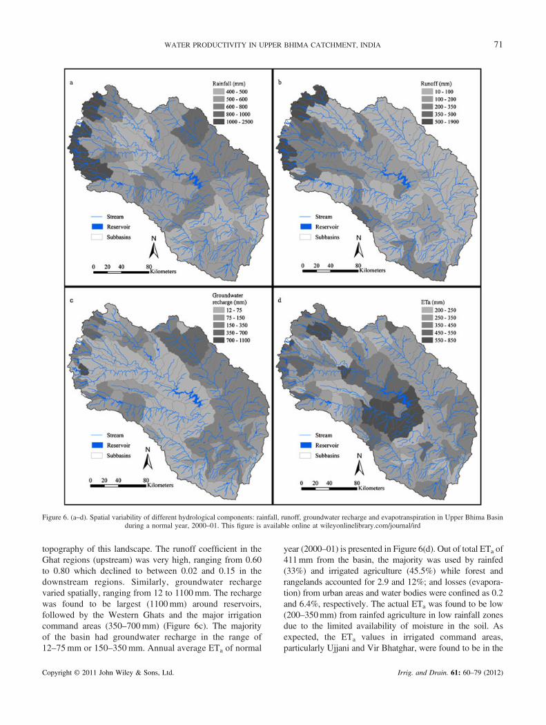
Figure 6. (a–d). Spatial variability of different hydrological components: rainfall, runoff, groundwater recharge and evapotranspiration in Upper Bhima Basinduring a normal year, 2000–01. This figure is available online at wileyonlinelibrary.com/journal/ird


topography of this landscape. The runoff coefficient in theGhat regions (upstream) was very high, ranging from 0.60to 0.80 which declined to between 0.02 and 0.15 in thedownstream regions. Similarly, groundwater rechargevaried spatially, ranging from 12 to 1100mm. The rechargewas found to be largest (1100mm) around reservoirs,followed by the Western Ghats and the major irrigationcommand areas (350–700mm) (Figure 6c). The majorityof the basin had groundwater recharge in the range of12–75mm or 150–350mm. Annual average ETa of normal


year (2000–01) is presented in Figure 6(d). Out of total ETa of411mm from the basin, the majority was used by rainfed(33%) and irrigated agriculture (45.5%) while forest andrangelands accounted for 2.9 and 12%; and losses (evapora-tion) from urban areas and water bodies were confined as 0.2and 6.4%, respectively. The actual ETa was found to be low(200–350mm) from rainfed agriculture in low rainfall zonesdue to the limited availability of moisture in the soil. Asexpected, the ETa values in irrigated command areas,particularly Ujjani and Vir Bhatghar, were found to be in the

Irrig. and Drain. 61: 60–79 (2012)


highest range of 550–850mm (Figure 6d). ETa in the upstreamWestern Ghats was found in the middle ranges (400–600mm)due to a combination of soil and land cover factors. The depthof soil in the Western Ghats is shallow and water‐holdingcapacity low compared to other parts of the basin. As a result,the potential for ETa is less in the Ghats during the non‐monsoon period. A large portion of theGhat area is covered byforests, where water can be extracted from subsurface layers tocontribute to ETa. Overall 79%of ETawas used by agriculturalcrops, while 15%was used by forest or rangelands and 6% lost(through evaporation) from urban areas and water bodies. Inother words, 46% of rainfall was used by agricultural crops.

Crop water productivity

Crop yield and WP were mapped spatially on a sub‐basinscale and are presented in Figures 7 and 8 for sorghum andsugarcane during wet (1999) and dry (2003) yearsrespectively. Crop productivity in different sub‐basins wasestimated based on yield and ETa from SWAT‐simulatedoutputs. The top two panels of Figure 7 show sorghum yieldand crop WP for 1999 and the lower panel yield and WP for2003. In a similar manner, results are presented forsugarcane in Figure 8.

The crop yields simulated by the model were foundcomparable with the actual yield obtained from theDepartment of Agriculture, Government of Maharashtra(http://www.mahaagri.gov.in) for different years. During anormal year (2000–01), the average simulated yields(σ, standard deviation) of sugarcane, sorghum and milletcrops were found as 40 (±19.1), 1.4 (±1.0) and 0.75 (±0.5)t ha¯1, respectively. Actual average yield (Department ofAgriculture, Government of Maharashtra, India) werereported as 90 (±13), 1.3 (±0.3), 1.1 (±0.4) t ha¯1, forsugarcane, sorghum and millet crops respectively. Themodel was set with a large acreage under sugarcane cropcompared to the actual area in 2000–01 (land useclassification was based on 2004–05). Water availabilityfor the sugarcane crop (modelled area) was not adequatewhich resulted in a lower crop yield (simulated) particularlyoutside the command area. Crop yields varied significantlyat both temporal and spatial scales.

Variations in yield were found to be very high forsorghum, as it ranged from 0.01 to 5.8 t ha¯1 yr¯1 at differentlocations in different rainfall years. During a wet year,the majority of the basin demonstrated yield in the range of1–3 t ha¯1, while the yield peaked in some irrigation projectsat 3–5.8 t ha¯1. During the dry year in 2003, crop yielddeclined to 0.5–1 t ha¯1 or less.

Sorghum WP in 1999 (wet year) varied from 0.01 to1.8 kg m¯3, with the majority of the area between 0.5 and0.9 kg m¯3. WP declined significantly during the dry year(2003) and the majority of the area had a WP below 0.5 kg


m¯3 with 70% of the basin below 0.2 kg m¯3. Sorghum yieldwas found to be high in irrigated command areas,particularly in middle reaches and in the downstream partof the basin possibly due to rainfall pattern, wateravailability in the soil and access to irrigation from canalsor groundwater. Despite high rainfall in the Western GhatsWP was found to be poor, probably due to comparativelyfewer number of rainy days, low soil water availability aswell as soil nutrient stress in agricultural fields.

The sugarcane yields within different sub‐basins showedthat the yields in irrigated command areas were as high as45–90 t ha¯1 during 1999 (wet year). Crop yields outside theirrigated command were, however, estimated to be very low(10–45 t ha¯1). During a dry year (2003), the range of cropyields reduced to 45–60 t ha¯1 in the irrigated command andbelow 20 t ha¯1 outside the command areas. During 2003,releases for irrigation from some major reservoirs (partic-ularly Ujjani) were curtailed significantly when somereservoirs ended up using dead storage for domestic needs.During 1999, WP for the sugarcane crop was found inthe range of 4–12 kg m¯3 in the majority of the basin, with8–12 kg m¯3 in canal‐irrigated commands. During 2003,the majority of the area had a WP of 1–4 kg m¯3, whilesome irrigated command areas or areas around reservoirsdemonstrated WP in the range of 4–8 kg m¯3.

The average water productivities were found as 2.9(±2.0) kg m¯3 for sugarcane, 0.51 (±0.3) kg m¯3 forsorghum and 0.30 (±0.1) kg m¯3 for millet crops. Theoptimum values of WP for sugarcane, sorghum and milletcrops were found when ETa was in the range of 1100–1200,300–400 and 400–500mm respectively. Immerzeel et al.(2008) reported similar WP for sugarcane in the UpperBhima but larger values (1.3 kg m¯3) for sorghum crops.The values for sorghum were comparable with the optimumWP, which indicates that Immerzeel et al. (2008) must haveestimated potential WP under no water or nutrient stress.Similar values for sorghum WP have been reported byDoorenbos and Kassam (1979) (0.60–1.0) and Mu et al.(2008) (0.65 kg m¯3) for China. In the case of pearl millet,Klaij and Vachaud (1992) reported a slightly higher range(0.5–1.1 kg m¯3) in Nigar (Rockstrom, 1995). Wheat hasbeen reported to be more productive when compared withother crops within India and elsewhere. For instance Muet al. (2008) reported 1.31 kg m¯3 in China which wastwice that of sorghum. In India, various values for wheatWP were reported as 0.86–1.31 kg m¯3 in Pantnagar(Mishra et al., 1995); 1.11–1.29 kg m¯3 in West Bengal(Bandyopadhyay and Mallick, 2003); 0.48–0.71 in UttarPradesh (Sharma et al., 2001); and 0.27–0.82 in Karnal(Sharma et al., 1990). A large gap among estimated andpotential (Immerzeel et al., 2008) and global waterproductivities clearly shows considerable scope for improve-ment which could be obtained through appropriate land and

Irrig. and Drain. 61: 60–79 (2012)

Figure 7. Yield and water productivity of sorghum crop in 1999 (wet year) and 2003 (dry year). This figure is available online at wileyonlinelibrary.com/journal/ird


water management practices, improved and drought‐tolerantcrop varieties, supplementary irrigation in rainfed areas,irrigation scheduling and improvement in irrigation efficien-cy and precision farming in irrigated lands.

Economic water productivity

The economic water productivity (EWP) is a function ofnet income and water used (Equations 1 and 2). The EWPwas determined for the Ujjani canal irrigated command,which is one of the largest and most important projects in


the basin. The irrigated area in the command varied from759 to 1005 km2 which accounted for 33–44% of irrigationpotential in the command. The sugarcane area accounted foran area similar to the irrigated area in the command.

In general, the net income from sugarcane (US$1394ha¯1)was tenfold that of millet (US$129 ha¯1) and twentyfold ofsorghum (US$67 ha¯1) (Table V). The water requirementof sugarcane was four times that of sorghum and millet.However, the water requirements of wheat and groundnutwere not significantly different from sorghum and millet,and the net incomes were comparable with millet and

Irrig. and Drain. 61: 60–79 (2012)

Figure 8. Yield and water productivity of sugarcane crop in 1999 (wet year) and 2003 (dry year). This figure is available online at wileyonlinelibrary.com/journal/ird


sugarcane, respectively. When compared for EWPET,groundnut was found the most productive, followed bysugarcane, wheat and millet.

Net income from the basin ranged from US$40.6 millionin a wet year to US$31.3million in a dry year (Table VI).The EWP of the basin was estimated with respect to actualwater input (EWPIP) and ranged between US$0.022m¯3 in awet year to US$0.036m¯3 in a dry year (Table VI). TheEWPIP was maximal during a dry year because ofsignificantly less water input (irrigation and effectiverainfall) than in a wet year. However, the water input during


a wet year was three times the total water available for thecrop in a dry year, and the net income was found to be only30% higher in a wet year than in a dry year. It means the WPwas more determined by water input during a year. The waterinput increased productivity to a certain extent and water inexcess affected the crop yield adversely. Vaidyanathan andSivasubramaniyan (2004) also reported similar ranges ofEWP in irrigated and rainfed areas between US$0.018–0.027and 0.012–0.032m¯3, respectively, for major river basins inIndia during 1991–1993. EWP in irrigated areas is found to belower than for rainfed crops at larger percentage area due to

Irrig. and Drain. 61: 60–79 (2012)

Table V. Evapotranspiration (year 2000–01) and net value of major crops in the Ujjani command

Crop grown Crop growingseason

Crop yield(t ha¯1)

ETa (mm) ETa under nostress condition (mm)

Water stressfactora

Income(US$ ha¯1)

Millet Kharif 1.7 398 306 0.0 129Sorghum Rabi 1.2 237 353 0.33 67Sugarcane Perennial 110 1418 1348 0.0 1394Groundnut Kharif 3.1 382 394 0.03 890Wheat Rabi 1.5 205 347 0.41 137

aStress factors 0 and 1 represent no stress and maximum stress situation during crop growth, respectively.

Table VI. VIEconomic water productivity in the Ujjani command (base line)

Year 1999–2000 2000–2001 2001–2002 2002–2003

Canal water released for irrigation (Mm3) 1530 848 519 697Effective rainfall (mm) 620 507 531 390Gross area cultivated (km2) Actual 1005 844 759 983

Modelled 4664 2618 1313 1755Net income generated (US$ million) Actual 40.7 36.5 32.0 31.4

Modelled 78.4 43.8 23.5 17.9EWPIP (US$ m¯3) Actual 0.022 0.033 0.044 0.036

Modelled 0.026 0.029 0.027 0.017


over‐irrigation and high conveyance and application losses(especially in canal command areas). Aggarwal et al. (2001)reported similar EWP (US$0.025–0.063m¯3) for paddy,wheat, mustard and cotton crops in kharif and larger EWP(US$0.10–0.13m¯3) in rabi under a surface irrigation systemin Sirsa district, Haryana, India.

Scenario analysis in the Ujjani command area

In order to understand the impact of various scenarios,the net income and EWP of major crops were used asindicators. Considering socio‐economic aspects, four sce-narios (Table VII) focusing on various crop diversificationoptions were evaluated for the Ujjani command. Theindicators for impact assessment were irrigable area, cropyields and the EWP (with respect to actual water input)which were compared with the baseline, i.e. actual valuesduring a year. All the indicators with respect to eachscenario during wet (1999–2000), normal (2000–01) anddry (2001–02 and 2002–03) years are shown in Table VII.

Scenario 1 included diversification from millet andsorghum to groundnut and wheat. The actual waterrequirements were not significantly different from thebaseline except that the sugarcane was prioritized evenduring dry years which resulted in no irrigation to wheatand groundnut during dry years or probably stressed duringnormal years. The level of stress was evidenced by lowcrop yields during normal and dry years than wet years.The area irrigated during a normal year was quite close to


the baseline, while net income increased to US$60millionas opposed to US$36.4million for current practices.During a wet year, net income almost quadrupled butduring a dry year, it matched the baseline. The EWPIP weresimilar during wet and normal years (US$0.058m¯3) andalmost twice the baseline. During a dry year, the EWPIP(US$0.040m¯3) was comparable with the baseline.

Scenario 2 aimed at maximizing irrigation intensity bydiversifying the sugarcane area into groundnut and wheatwhile maintaining sorghum and millet crops. The irrigationpotential was substantially higher than the baseline areaswhich can be attributed to some limitations in the model.Although attempts were made to account for spatialvariability in various parameters, the model was unable toincorporate the actual spatial pattern of land use, irrigationefficiencies and water stress over the command. The modelprioritizes irrigation by limiting the area or stress to adefined limit while in practice the stress varies from field tofield. Groundwater use in the model was limited to ashallow aquifer while in practice the groundwater isexploited from a deep aquifer. This limitation might haveled to underestimation of irrigation potential during dryyears. The net income under this scenario (US$116million)was almost three times the baseline during wet and normalyears. During a dry year, it declined to US$45 millionwhich is 25% higher than the baseline. As opposed toScenario 1, this scenario improved the EWPIP significantlyduring normal and dry years and ranged fromUS$0.035m¯3 (wet year) to US$0.066m¯3 (normal year).

Irrig. and Drain. 61: 60–79 (2012)

Table VII. Comparison of various indicators under various scenarios in the Ujjani command

Parameters Scenarios

Baseline Scenario 1 Scenario 2 Scenario 3 Scenario 4

Year 1999–2000 (wet year)Kharif crops Area km2 (yield t ha¯1) Millet 2260 (2.0) – 1364 (0.7) – –

Groundnut – 1491 (1.9) 1364 (2.1) 2827 (2.2) 1435 (2.6)Rabi crops Area km2 (yield t ha¯1) Sorghum 2260 (1.7) – 2267 (0.8) – –

Wheat – 1491 (1.1) 2217 (1.3) 3896 (1.3) 3107 (1.4)Perennial Area km2 (yield t ha¯1) Sugarcane 145 (82) 413 (127) – – –Total area (km2) 4665 3395 7182 6723 4542Net income (US$ million) 78.4 155 111 213 142Water used (Mm3) IP 3021 2711 3203 3283 2419

ET 1640 1328 1865 1369 1459Economic water productivity (US$ m¯3) EWP(IP) 0.026 0.057 0.035 0.065 0.059

EWP(ET) 0.048 0.117 0.059 0.155 0.097Year 2000–2001 (normal year)Kharif crops Area km2 (yield t ha¯1) Millet 1269 (2.5) – 899 (1.7) – –

Groundnut 0 879 (3.2) 1883 (3.3) 1207 (4.0)Rabi crops Area km2 (yield t ha¯1) Sorghum 1269 (1.3) – 1292 (1.2) – –

Wheat 317 (1.3) 1264 (1.5) 2280 (1.5) 1853 (1.6)Perennial Area km2 (yield t ha¯1) Sugarcane 81 (73) 413 (73) – – –Total area (km2) 2619 731 4334 4163 3060Net income (US$ million) 43.8 61 116 204 163Water used (Mm3) IP 1532 1057 1748 1802 1459

ET 944 642 1187 999 1061Stress factor (−) 0.14 0.19 0.22 0.37 0.0Economic water productivity (US$ m¯3) EWP(IP) 0.029 0.058 0.066 0.113 0.112

EWP(ET) 0.046 0.095 0.097 0.204 0.154Year 2001–2002 (dry year)Kharif crops Area km2 (yield t ha¯1) Millet 636 (2.7) – 321 (1.4) – –

Groundnut – 0 314 (2.7) 674 (2.8) 399 (3.0)Rabi crops Area km2 (yield t ha¯1) Sorghum 636 (1.4) – 901 (1.1) – –

Wheat – 0 881 (1.6) 1612 (1.6) 1321 (1.9)Perennial Area km2 (yield t ha¯1) Sugarcane 41 (66) 251 (99) – – –Total area (km2) 1313 251 2417 2286 1720Net income (US$ million) 23.5 30 45 77 58Water used (Mm3) IP 879 652 856 877 731


EWP(ET) 0.047 0.084 0.075 0.165 0.112Year 2002–2003 (dry year)Kharif crops Area km2 (yield t ha¯1) Millet 850 (1.4) – 321 (1.4) – –

Groundnut – 0 313 (3.0) 660 (3.0) 416 (3.2)Rabi crops Area km2 (yield t ha¯1) Sorghum 850 (1.3) – 1093 (1.3) – –

Wheat – 0 1070 (1.6) 1894 (1.7) 1543 (2.0)Perennial Area km2 (yield t ha¯1) Sugarcane 55 (60) 296 (93) – – –Total area (km2) 1755 296 2797 2554 1959Net income (US$ million) 17.9 32 54 85 69Water used (Mm3) IP 1050 812 944 954 859


EWP(ET) 0.026 0.073 0.073 0.193 0.105


In Scenario 3, the irrigated area was maximized byreplacing existing crops with groundnut and wheat. Thisscenario enhanced irrigation intensity (ratio of area irrigated


to command area) to 300% during a wet year and to 200%during a normal year. Simultaneously, the range of netincome was enhanced between US$77million (dry year) to

Irrig. and Drain. 61: 60–79 (2012)


US$213million (wet and normal years) which was almosttwo to six times the baseline WP. The EWPIP increasevaried from US$0.065m¯3 (wet year) to US$0.113m¯3

(normal year), demonstrating a threefold increase inproductivity under this scenario.

Under Scenario 4, irrigation was optimized to provide astress‐free environment for the crops adopted in Scenario 3in order to maximize returns per unit of land. As a result,irrigation intensity declined by 100% when compared withScenario 3. The net income (US$58–162 million) was alsofound to be significantly less than the income underScenario 3, yet it was two to four times the baselineincome. Since the water used was less than under Scenario3, the EWPIP was comparable with Scenario 3.

All the scenarios led to improvement in irrigationintensity, net income and economic WP over baseline.Scenario 3 demonstrated the largest irrigation intensity, netincome and EWP followed by Scenarios 4, 2 and 1. Itmeans that the groundnut and wheat crops with limitedirrigation supplies of four and six irrigations, respectively,were the best option out of the alternatives assessed in thepresent study. The water‐stress‐free environment for thesecrops improved the yield but it led to a reduction inirrigation intensity and net income as in Scenario 4. Thepriority given to sugarcane in Scenario 1 led to asubstantial reduction in WP by ignoring irrigation suppliesto wheat and groundnut during dry years. However, asScenario 2 contained mixed cultivation of millet orsorghum along with high‐value crops targeting a morediverse and resilient cropping system. Sorghum and milletare both low‐value crops but have high tolerance to water‐stress situations. Therefore, although the WP values arelower, the scenario is good during water‐stress years. TheEWP based on evapotranspiration was 1.5–2.4 times theEWP based on actual water utilized, suggesting that thepotential for EWP in the basin during a normal year wasUS$0.204m¯3, leading to a total net income of US$204million. It may be noted that the study consideredsupport prices. The actual value of crops may varyaccording to market conditions, which is predominantlycontrolled by supply and demand characteristics andseveral other externalities.

SUMMARY AND CONCLUSIONS

The Upper Bhima River Basin is facing both episodic andchronic water shortages due to intensive development indomestic, industrial and irrigation water needs. With ashrinking allocation to irrigation, there is a need tointroduce water management interventions with optimumreturns. In this study, the hydrological processes of theUpper Bhima River Basin were modelled using the


distributed hydrologic model, SWAT. The spatial patternof WP of major crops was analysed with the aim ofimproving the economic efficiency of water use in theirrigated area. The key findings of this study are:

• rainfall in the basin ranged from 450 to 5000mm, themajority of which occurred in the Western Ghatswithin 3–4months. During a normal year, out ofaverage rainfall of 32 400Mm3 (711mm), 12.8 and21% were stored in surface and ground reserves,respectively, and 7% resulted in surface runoff out ofthe basin;

• evapotranspiration is the major sink component in thehydrological balance (60%), where 46% was used byagricultural crops;

• the WP of major crops, sugarcane, sorghum and millet,was found to be 2.9, 0.51 and 0.30 kg m¯3,respectively. Crop productivity in the basin was foundin the lower range when compared with potential andglobal values. The findings suggested that there was apotential to improve further;

• during a normal year, the net returns and EWP of theUjjani Irrigation Scheme were found to be US$36.6million and US$0.033m¯3, respectively, whichcould be further improved to US$204 million and US$0.204m¯3, by diversifying existing crops (sorghum,millet and sugarcane) to groundnut and wheat crops.

Physical water scarcity was, however, not the onlyfactor for poor WP in the basin. High nutrient losses inupstream locations due to heavy runoff and inefficientwater utilization in water‐rich command areas are otherimportant factors. There is potential to increase the WP ofdifferent crops in the basin as the productivity of cerealcrops was very low. Better on‐farm water managementpractices, crop diversification, supplemental irrigation torainfed areas and other technological innovations could beimplemented.

ACKNOWLEDGEMENTS

This research was supported by a grant (LWR/2003/026)from the Australian Centre for International AgriculturalResearch (ACIAR). The views expressed in this article arethose of authors alone and do not necessarily represent theofficial position of the World Bank. The authors would liketo thank Dr W.W. Immerzeel for his support in the settingup the model. The authors are also grateful for the supportprovided by the Irrigation Project and Water ResourcesInvestigation Circle, Pune, India, Hydrology Surface DataCentre, Nashik, India and Ujjani Command Area Develop-ment Authority, Solapur, India.

Irrig. and Drain. 61: 60–79 (2012)


REFERENCES

Aggarwal PK, Roeter RP, Kalra N, Van Keulen H, Hoanh CT, Van Laar HH(eds). 2001. Land use analysis and planning for sustainable food security:with an illustration for the state of Haryana, India. Indian ResearchInstitute: New Delhi; International Rice Research Institute: Los Baños;Wageningen University and Research Center: Wageningen, 1–167.

Arnold JG, Srinivasan P, Muttiah RS, Williams JR. 1998. Large areahydrologic modeling and assessment. Part I. Model development.Journal of the American Water Resources Association 34: 73–89.

Bandyopadhyay PK, Mallick S. 2003. Actual evapotranspiration and cropcoefficients of wheat (Triticum aestivum) under varying moisture levelsof humid tropical canal command area. Agricultural Water Management59: 33–47.

Bastiaanssen WGM, Menenti M, Feddes RA, Holtslag AAM, 1998a. TheSurface Energy Balance Algorithm for Land (SEBAL): Part 1formulation. Journal of Hydrology 212–213: 198–212.

Bastiaanssen WGM, Pelgrum H, Wang J, Ma Y, Moreno J, Roerink GJ,van der Wal T. 1998b. The Surface Energy Balance Algorithm for Land(SEBAL): Part 2 validation. Journal of Hydrology 212–213: 213–229.

Bastiaanssen WGM, Noordman EJM, Pelgrum H, Davids G, Allen RG.2005. SEBAL for spatially distributed ET under actual management andgrowing conditions. ASCE Journal of Irrigation and DrainageEngineering 131(1): 85–93.

Bosch NS. 2008. The influence of impoundments on riverine nutrienttransport: an evaluation using the Soil and Water Assessment Tool.Journal of Hydrology 355: 131– 147.

Bouman BAM. 2007. A conceptual framework for the improvement ofcrop water productivity at different spatial scales. Agricultural Systems93: 43–60.

Challa O, Gajbhiye KS, Velayutham M. 1999. Soil Series of Maharashtra.NBSS Publication No. 79. National Bureau of Soil Survey and Land UsePlanning (BSS&LUP): Nagpur; 428 pp.

Chiew FHS, Peel MC, Western AW. 2002. Application and testing of thesimple rainfall‐runoff model SIMHYD. In Mathematical Models ofSmall Watershed Hydrology and Applications, Singh VP, Frevert DK(eds). Water Resources Publications: Littleton, Colo.; 335–367.

Doorenbos I, Kassam AH. 1979. Yield response to water. FAO Irrig. andDrain. Paper 33, Rome, 1–193.

Gassman PW, Reyes MR, Green CH, Arnold JG. 2007. The Soil and WaterAssessment Tool: historical development, application and futureresearch directions. Transactions of the ASABE 50(4): 1211–1250.

Gaur A, Acharya S, Turral H, McCornick PG. 2007. Implications ofdrought and water regulation in the Krishna basin, India. InternationalJournal of Water Resources Development 23(4): 583–589.

Geza M, McCray JE. 2008. Effects of soil data resolution on SWAT modelstream flow and water quality predictions. Journal of EnvironmentalManagement 88: 393–406.

Government of India. 2001. General population tables. Office of theRegistrar General and Census Commissioner, Ministry of Home Affairs:New Delhi.

Government of Maharashtra. 2005. Report on Water Audit of IrrigationProjects in Maharashtra 2004–05. Water Resources Department: Mumbai.

Green CH, Griensven AV. 2008. Autocalibration in hydrologic modeling:using SWAT2005 in small‐scale watersheds. Environmental Modelling& Software 23: 422–434.

Groundwater Resources of India (Central Ground Water Board) 1995.Ground Water Profiles (State wise) (online). (Ministry of WaterResources, Government of India). Available at http://cgwb.gov.in/(accessed 4 May 2010).

Gunnel Y. 1997. Relief and climate in South Asia: the influence of theWestern Ghats on the current climate pattern of Peninsular India.International Journal of Climatology 17: 1169–1182.


Immerzeel WW, Gaur A, Zwart SJ. 2008. Integrating remote sensing and aprocess‐based hydrological model to evaluate water use and productivityin a south Indian catchment. Agricultural Water Management 95: 11–24.

Kang MS, Park SW, Lee JJ, Yoo KH. 2006. Applying SWAT for TMDLprograms to a small watershed containing rice paddy fields. AgriculturalWater Management 79: 72–92.

Kannan N, White SM, Worrall F, Whelan MJ. 2007. Hydrologicalmodelling of a small catchment using SWAT‐2000 – ensuring correctflow partitioning for contaminant modeling. Journal of Hydrology 334:64–72.

Kijne JW, Barker R, Molden D. 2003. Water Productivity in Agriculture:Limits andOpportunities for Improvement. CAB International:Wallingford.

Klaij MC, Vachaud G. 1992. Seasonal water balance of a sandy soil inNiger cropped with pearl millet, based on profile moisture measure-ments. Agricultural Water Management 21: 313–330.

Loeve R, Dong B, Molden D, Li YH, Chen CD, Wang JZ. 2004. Issues ofscale in water productivity in the Zhanghe irrigation system: implicationsfor irrigation in the basin context. Paddy and Water Environment 2(4):227–236.

Luo Y, He C, Sophocleous M, Yin Z, Hongrui R, Ouyang Z. 2008.Assessment of crop growth and soil water modules in SWAT2000 usingextensive field experiment data in an irrigation district of the YellowRiver Basin. Journal of Hydrology 352: 139–156.

Mishra HS, Rathore TR, Tomar VS. 1995. Water use efficiency of irrigatedwheat in the Tarai region of India. Irrigation Science 16: 75–80.

Molden D. 1997. Accounting for water use and productivity. In SWIMPaper 1. IIMI: Colombo.

Molden D, Sakthivadivel R. 1999. Water accounting to assess use andproductivity of water. International Journal of Water ResourcesDevelopment 15(1 and 2): 55–71.

Mu J, Khan S, Hanjra MA, Wang H. 2008. A food security approach toanalyze irrigation efficiency improvement demands at the country level.Irrigation and Drainage 58(1): 1–16.

Nash JE, Sutcliffe JV. 1970. River flow forecasting through conceptualmodels, 1. A discussion of principles. Journal of Hydrology 10: 282–290.

National Water Development Agency. 2003. Water balance study of theUpper Bhima subbasin of the Krishna Basin. Technical Study No. 77.National Water Development Agency, Ministry of Water Resources,Government of India, New Delhi.

Neena D. 1998. Inter‐state variation in cropping pattern in India. IndianJournal of Regional Science 30: 57–69.

Neitsch SL, Arnold JG, Kiniry JR, Williams JR, King KW. 2005. Soil andwater assessment tool. Theoretical documentation, Version 2005.Grassland, Soil and Water Research Laboratory, Agricultural ResearchService and Blackland Research Centre, Texas Agricultural Experimen-tal Station: TX.

Rabus B, Eineder M, Roth A, Bamler R. 2003. The shuttle radartopography mission – a new class of digital elevation models acquired byspaceborne radar. Photogrammetric Engineering and Remote Sensing57: 241–262.

Rockstrom J. 1995. Biomass production in dry tropical zones: how toincrease water productivity. Land and Water Integration and River BasinManagement. FAO Land and Water Bulletin, 31–47.

Schuol J, Abbaspour KC, Srinivasan R, Yang H. 2008. Estimation offreshwater availability in the West African sub‐continent using theSWAT hydrologic model. Journal of Hydrology 352: 30–49.

Sharma KD, Kumar A, Singh KN. 1990. Effect of irrigation scheduling ongrowth, yield and evapotranspiration of wheat in sodic soils. AgriculturalWater Management 18: 267–276.

Sharma KS, Samra JS, Singh HP. 2001. Influence of boundaryplantation of poplar (Populus deltoides M.) on soil‐water use andwater use efficiency of wheat. Agricultural Water Management 51:173–185.

Irrig. and Drain. 61: 60–79 (2012)


Srinivasan R, Ramanarayanan TS, Arnold JG, Bednarz ST. 1998. Largearea hydrologic modeling and assessment part II: model application.Journal of American Water Resources Association 34: 91–101.

Tuong TP, Bouman BAM. 2003. Rice productivity in water‐scarceenvironments. In Water Productivity in Agriculture: Limits andOpportunities for Improvement, The Comprehensive Assessment ofWater Management in Agriculture Series, vol. 1, Kijne JW, Barker R,Molden D (eds). CABI Publishing: Wallingford, UK; 1–342.

Ullrich A, Volk M. 2009. Application of the Soil and Water AssessmentTool (SWAT) to predict the impact of alternative management practiceson water quality and quantity. Agricultural Water Management 96:1207–1217.


Vaidyanathan A, Sivasubramaniyan K. 2004. Efficiency of water use inagriculture. Economic and Political Weekly 3 July.

Van Griensven A, Meixner T, Grunwald S, Bishop T, Diluzio M, SrinivasanR. 2006. A global sensitivity analysis tool for the parameters of multi‐variable catchment models. Journal of Hydrology 324(1–4): 10–23.

Williams JR, Arnold JG, Kiniry JR, Gassman PW, Green CH. 2008.History of model development at Temple, Texas. Hydrological ScienceJournal 53(5): 948–960.

Yang Q, Meng F‐R, Zhao Z, Chow TL, Benoy G, Rees HW, Bourque CP‐A. 2009. Assessing the impacts of flow diversion terraces on streamwater and sediment yields at a watershed level using SWAT model.Agriculture, Ecosystems and Environment 132: 23–31.

Irrig. and Drain. 61: 60–79 (2012)

spatial mapping of agricultural water productivity...

Documents