spatial join techniques
TRANSCRIPT

Spatial Join Techniques
EDWIN H. JACOX and HANAN SAMET
Computer Science Department
Center for Automation Research
Institute for Advanced Computer Studies
University of Maryland
College Park, Maryland 20742
[email protected] and [email protected]
A variety of techniques for performing a spatial join are reviewed. Instead of just summarizingthe literature and presenting each technique in its entirety, distinct components of the differenttechniques are described and each technique is decomposed into an overall framework for per-forming a spatial join. A typical spatial join technique consists of the following components:partitioning the data, performing internal memory spatial joins on subsets of the data, and check-ing if the full polygons intersect. Each technique is decomposed into these components and eachcomponent is addressed in a separate section so as to compare and contrast the similar aspects ofeach technique. The goal of this survey is to describe algorithms within each component in detail,comparing and contrasting competing methods, thereby enabling further analysis and experimen-tation with each component and allowing for the best algorithms for a particular situation to bebuilt piecemeal, or, even better, enabling an optimizer to choose which algorithms to use.
Categories and Subject Descriptors: H.2.4 [Systems]: Query processing; H.2.8 [Database Ap-
plications]: Spatial databases and GIS
General Terms: Algorithms,Design
Additional Key Words and Phrases: external memory algorithms, plane-sweep, spatial join
1. INTRODUCTION
This article presents an in-depth survey and analysis of spatial joins. A large bodyof diverse literature exists on the topic of spatial joins. The goal of this article isnot only to survey the literature on spatial joins, but also to extract algorithms andtechniques from the literature and to present a coherent description of the stateof the art in the design of spatial join algorithms. Frequently, an article presentsa complete framework for performing a spatial join. Instead of summarizing eachcomplete framework individually, we decompose them into components in two ways.First, if several methods are similar, then a common algorithm is extracted fromthe frameworks to show specifically how each framework differs from the others.
Permission to make digital/hard copy of all or part of this material without fee for personalor classroom use provided that the copies are not made or distributed for profit or commercialadvantage, the ACM copyright/server notice, the title of the publication, and its date appear, andnotice is given that copying is by permission of the ACM, Inc. To copy otherwise, to republish,to post on servers, or to redistribute to lists requires prior specific permission and/or a fee.c© 2006 ACM 0362-5915/2006/0300-0001 $5.00
ACM Transactions on Database Systems, Vol. V, No. N, November 2006, Pages 1–45.

2 · E.H. JACOX and H. SAMET
Table I. Components of spatial join algorithms.Internal Memory A.3 Nested Loop Join [Mishra and Eich 1992]Methods A.3 Index Nested-Loop Join [Elmasri and Navathe 2000]
3.1 Plane Sweep [Arge et al. 1998; Preparata and Shamos 1985]3.2 Z-Order [Aref and Samet 1994b; Orenstein 1986]
Section 4.1 ExternalMemory Methods
4.1.1 Hierarchical Traversal [Brinkhoff et al. 1993; Gunther 1993;Huang et al. 1997b; Kim et al. 1995]
(Both Datasets In-dexed)
4.1.2 Non-Hierarchical Methods [Harada et al. 1990; Kitsuregawaet al. 1989]4.1.3 Multi-Dimensional Point Methods [Song et al. 1999]
Section 4.2 External 4.2.1 Construct a Second Index [Lo and Ravishankar 1994]Memory Methods 4.2.2 The Index as Partitioned Data [van den Bercken et al. 1999;
Mamoulis and Papadias 2003](One Dataset Not In-dexed)
4.2.3 The Index as Sorted Data [Arge et al. 2000; Gurret andRigaux 2000]
Appendix 4.3 External B.1 External Plane Sweep [Jacox and Samet 2003]Memory Methods 4.3.1 Generic Partitioning Algorithm(Neither Dataset B.2 Grid Partitioning [Patel and DeWitt 1996; Zhou et al. 1997]Indexed) B.3 Strip Partitioning [Arge et al. 1998]
B.4 Size Partitioning [Koudas and Sevcik 1997; Arge et al. 1998]B.5 Data Partitioning [Lo and Ravishankar 1995; 1996]
Appendix D D.1 Ordering Candidate Pairs [Abel et al. 1999]Refinement D.2 Polygon Intersection Test [Preparata and Shamos 1985;
Brinkhoff et al. 1994]D.3 Alternate Intersection Test [Brinkhoff et al. 1994]
Table II. Spatial join issues.Fundamentals and Section 2 Spatial Join BasicsConcepts Appendix A.1 Minimum Bounding Rectangles
Appendix A.2 Linear Orderings
Processing Issues 4.1.4 Joining Data Nodes
Partitioning Issues 4.3.2 Determining the Number of Partitions4.3.3 Repartitioning4.3.4 Avoiding Duplicate Results
Section 6 Uniform Dataset Estimates [Aref and Samet 1994a]Selectivity Estimation Non-Uniform Dataset Estimates [Belussi and Faloutsos 1995; Das
et al. 2004; Faloutsos et al. 2000; Mamoulis and Papadias 2001b]
Appendix C AlternateFiltering Techniques
C.1 False Hit Filtering [Brinkhoff et al. 1993; Koudas and Sevcik1997; Veenhof et al. 1995; Zimbrao and de Souza 1998]C.2 True Hit Filtering [Brinkhoff and Kriegel 1994a]C.3 Non-Blocking Filtering [Luo et al. 2002]
For instance, there exist several methods for performing a spatial join on R-trees[Guttman 1984], each using a hierarchical traversal method. From these differentalgorithms, we create a generic hierarchical traversal algorithm and show how eachmethod slightly varies the generic algorithm (see Section 4.1.1). Thus, each methodis presented in a simpler manner that allows it to be more thoroughly comparedand contrasted with similar algorithms. By doing so, the strengths and weaknessesof each competing algorithm become more apparent. The various components aretabulated in Table I along with the sections in which they are discussed. The secondapproach to decomposing the various methods is to extract common issues from
ACM Transactions on Database Systems, Vol. V, No. N, November 2006.

Spatial Join Techniques · 3
Table III. Specialized spatial joins.Section 5.1 MultiwaySpatial Joins
5.1.1 Multiway Indexed Nested Loop [Mamoullis and Papadias1998; Mamoulis and Papadias 2001a; Papadias et al. 1998]5.1.2 Multiway Hierarchical Traversal [Mamoullis and Papadias1998; Mamoulis and Papadias 2001a; Papadias et al. 1998]
Section 5.2 Parallel Parallel Hierarchical Traversal [Brinkhoff et al. 1996]Spatial Joins Parallel Grid Partitioning Methods [Luo et al. 2002; Patel and
DeWitt 2000; Zhou et al. 1997]Hypercube Spatial Joins [Hoel and Samet 1994]
Section 5.3 DistributedSpatial Joins
Distributed Filter and Refine [Abel et al. 1995; Mamoulis et al.2003]
each and address these issues in separate sections. For example, many of the spatialjoin methods for handling unindexed data must deal with the issue of removingduplicate results from the different stages of spatial join processing. Rather thanseparately show how each framework handles duplicate results, different techniquesfor handling duplicate results are described in a separate section (Section 4.3.4).The sections dealing with issues that arise in algorithms are tabulated in Table II.Furthermore, spatial joins for specialized environments are discussed in separatesections, as tabulated in Table III.
The rest of the paper is organized as follows. Section 2 defines the spatial join op-eration and discusses design parameters that influence the performance of a spatialjoin. Typically, a spatial join is performed in two stages: the filter stage in whichcomplicated polygonal objects are approximated by rectangles and the refinement
stage which removes any results produced during the filtering stage that do notsatisfy the join condition [Orenstein 1989b]. Section 3 describes internal memoryfiltering techniques, while Section 4 describes external memory filtering techniques.Section 5 explains how spatial joins are handled in specialized situations, such as inparallel architectures, while Section 6 discusses selectivity estimation. Concludingremarks are drawn in Section 7. In addition, Appendix A describes the followingtwo concepts that are important to many spatial join algorithms: the minimum
bounding rectangle (also known as a minimum bounding box ) and linear orderings.Appendix B provides details of the methods that do not rely on the input datasetsbeing indexed. The remaining appendices elaborate further on the filter and refinestages. In particular, Appendix C presents extended or alternate filtering tech-niques, while Appendix D discusses the refinement phase.
2. SPATIAL JOIN BASICS
Given two datasets of multi-dimensional objects in Euclidean space, a spatial joinfinds all pairs of objects satisfying a given relation between the objects that involvesthe values of their spatial components, such as intersection. For example, a spatialjoin answers such queries as find all of the rural areas that are below sea level,given an elevation map and a land use map [Veenhof et al. 1995]. To illustrate theconcept further, a simplified version of a spatial join is as follows: given two sets ofrectangles, R and S, find all of the pairs of intersecting rectangles between the twosets, that is, for each rectangle r in dataset R, find each intersecting rectangle, s,from dataset S, as illustrated in Figure 1. The general spatial join problem, also
ACM Transactions on Database Systems, Vol. V, No. N, November 2006.

4 · E.H. JACOX and H. SAMET
r1s2
y
x
s3
r3r2s1
Fig. 1. A spatial join to find the intersecting objects of datasets R, consisting of objects r1, r2,and r3, and S, consisting of objects s1, s2, and s3, will report the intersection of objects r1/s2,r2/s2, r2/s3 and r3/s2.
known as a spatial overlay join, extends the simplified version in several ways:
(1) The datasets can be objects other than rectangles such as points, segments, orpolygons 1.
(2) The datasets might have more than two dimensions 2.
(3) The relationship between pairs of objects can be any relation between theobjects that involves the values of the spatial components, such as intersection,nearness, enclosure, or a directional relation (for example, find all pairs ofobjects such that r is northwest of s [Zhu et al. 2001]).
(4) There might be more than two datasets in the relation (a multiway spatial join)or only one dataset (a self spatial join).
The problem of spatial join has been the subject of much attention in fields otherthan spatial databases. In particular, its solutions make use of the same principlesas interference detection in robotics applications (for example, [Gottschalk et al.1996]), game programming (for example, [Ulrich 2000]), and design rule checkingin VLSI applications (for example, [Rosenberg 1985]). These topics are beyond thescope of this review, but for more details, the interested reader should consult textssuch as [Samet 2006].
Spatial joins are distinguished from a standard relational join [Mishra and Eich1992] in that the join condition involves the multi-dimensional spatial attribute ofthe joined relation. This property prevents the use of the more sophisticated rela-tional join algorithms. For instance, because the data objects are multi-dimensional,there is no ordering of the data that preserves proximity. Relational join techniquesthat rely on sorting the data, such as the sort-merge join [Mishra and Eich 1992],work because neighboring objects (those with the next higher and lower value) areadjacent to each other in the ordering. However, in more than one dimension, thedata can not be sorted so that this property holds for all directions and dimensions.For example, in two dimensions, the left and right neighbors can be adjacent to an
1An extensive amount of research has also examined the related operation, the segment join[Balaban 1995; Brinkmann and Hinrichs 1998; Chazelle and Edelsbrunner 1992; Mairson andStolfi 1988; van Oosterom 1994], and the more general overlay operation which also addresses theeffects of the result of the spatial join on the way in which the combined attributes of the join arehandled [van Roessel 1987; 1991; 1994].2A one dimensional version of the spatial join would be an interval join [Enderle et al. 2004].
ACM Transactions on Database Systems, Vol. V, No. N, November 2006.

Spatial Join Techniques · 5
object in an ordering, but then the top and bottom neighbors will need to go else-where in the order (see Appendix A.2 for a further discussion of multi-dimensionalorderings).
Other relational join techniques are also inapplicable because the data objectsmight have extent. For example, equijoin techniques [Mishra and Eich 1992] (forexample, hash joins), will not work with spatial data because they rely on groupingobjects with the same value, which is not possible when the objects have extent.This is the same reason that equijoin techniques will not work with intervals (extentin one dimension) or inequalities. As an example, for a one-dimensional hash joinon datasets R and S, a group of objects from R is mapped to the same bucket,G, if their keys, key, are mapped by the hash function f(key) to the same value.An object g in bucket G can only be paired with an object from S whose key isalso mapped to the same value (f(key)) by the same hash function. This propertydoes not hold for objects with extent, such as a rectangle, because the objects canoverlap each other and a disjoint grouping might not exist. In fact, an object fromdataset R could potentially intersect every object from dataset S. Because of thesetwo factors (that is, failure to satisfy proximity preservation and extent) relationaljoin algorithms cannot be used directly to perform a spatial join.
The computational geometry approach to solving the simplified spatial join (atwo-set rectangle intersection) is to use a plane-sweep technique [Preparata andShamos 1985] (see Section 3.1). In order to use the plane-sweep method for ageneral spatial join, two problems must be overcome: the objects are not necessarilyrectangles and there might not be sufficient internal memory for the plane-sweepalgorithm. Furthermore, calculating whether two complex objects satisfy the joincondition, such as intersection, can be an expensive operation, and performing asfew of these operations as possible improves overall performance. To overcome theseproblems, a spatial join is typically performed using a two stage filter-and-refineapproach [Orenstein 1989b].
In the filter-and-refine approach, the spatial join is first solved using approxi-mations of the objects in the filtering stage and any incorrect results due to theapproximations are removed in the refinement stage using the full objects 3. Inthe filtering stage, objects are typically approximated using minimum bounding
rectangles (see Appendix A.1), hereafter referred to as MBRs, which require lessstorage space than the full object, resulting in faster processing and less expensiveI/O operations 4. For example, GIS objects might be polygons, each consisting ofthousands, or even millions, of points. Reading these objects in and out of memorycould easily be the dominant cost of performing a spatial join, depending upon theavailable amount of internal memory and the ratio of I/O to CPU performance,whereas a filter-and-refine approach alleviates this problem. Furthermore, a spatialjoin on rectangles presents a more tractable problem. For smaller datasets, thefiltering stage of the spatial join can be solved using internal memory techniques,which are described in Section 3. For larger datasets, external (secondary) memory
3While the filter and refine stages can be considered two phases of one technique, Park et al. [1999]propose separating the filter and refinement steps for query optimization so that each stage canbe combined with non-spatial queries.4Other approximations also can be used (see Appendix C).
ACM Transactions on Database Systems, Vol. V, No. N, November 2006.

6 · E.H. JACOX and H. SAMET
techniques are required for the filtering stage, which are described in Section 4.
The output of the filtering stage is a list of all pairs of objects whose approxi-mations satisfy the join condition, which is referred to as the candidate set, and istypically represented by pairs of object ids. The candidate set includes all of thedesired pairs, those whose full objects satisfy the join condition, but also includespairs whose approximations satisfy the join condition, but whose full objects do not.The extra pairs appear because of the inaccuracy of the object approximations (seeAppendix A.1). The purpose of the refinement stage is to remove the undesiredpairs using the full objects, producing the final list of object pairs that satisfy thegiven join condition. Refinement techniques are described in Appendix D.
As mentioned above, the dominant cost of a spatial join with very large objectscan be the I/O cost of reading the large objects, depending upon the amountof internal memory and the ratio of I/O to CPU performance. Early filteringtechniques were dominated by I/O costs [Brinkhoff et al. 1993]. Later techniqueshave improved I/O performance so that it is no longer an axiom that I/O costsdominate the CPU costs [Patel and DeWitt 1996]. Even though filtering reducesthe I/O costs, reading large objects can still be the major cost of the refinementstage, which is generally more expensive than the filtering stage [Patel and DeWitt1996]. Furthermore, while the performance improvement from using a filter-and-refine approach might be obvious for very large objects, it remains an open questionas to whether it is the best approach for smaller, simpler objects. As an exampleof an alternative approach, Zhu et al. [2000a; 2000b] have proposed methods forextending the plane-sweep algorithm (Section 3.1) to trapezoids and recti-linearpolygons, thereby avoiding the need for the filter-and-refine approach for objectshaving such shapes.
Throughout the review of the spatial join techniques, we do not discuss experi-mental results. Most of the methods described in this survey were shown to outper-form some other method. Unfortunately, we found it difficult to compare methodsusing only the literature since the techniques are compared with one or no othertechnique, and the implementations of the techniques can vary dramatically, whichhas a large impact on the experimental results. Furthermore, the variety of com-puter hardware, software and networks used make it difficult to compare resultsbetween methods. For these reasons, we do not discuss most experimental results.
Also, to simplify the discussion of the techniques, it is assumed that the data istwo dimensional and that we are interested in determining pairs of intersecting ob-jects. Both of these assumptions are common in the literature. The two-dimensionalassumption is made because the applications of these techniques to higher dimen-sional data has not been extensively addressed in the literature and many of thetechniques presented might not work or might not perform well in higher dimen-sions. The intersection assumption is made only to simplify the discussion. Webelieve that this assumption does not effect the generality of the algorithms. Forexample, a nearness relation can easily be calculated by extending the size of theMBRs so that nearness is calculated by an intersection test [Koudas and Sevcik1998]. However, for some predicates, such as a directional predicate, the algorithmsneed to be modified appropriately. For instance Zhu et al. [2001] use a modifiedplane-sweep algorithm (see Section 3.1) to search for all objects in the desired di-
ACM Transactions on Database Systems, Vol. V, No. N, November 2006.

Spatial Join Techniques · 7
rection for a directional predicate. When appropriate, a generic join condition isused, rather than intersection.
Furthermore, although many spatial join techniques depend on spatial indices,the discussion of spatial indices is left to other work [Gaede and Gunther 1998;Samet 1990]. Knowledge of these structures can be crucial to a deeper understand-ing of many of the techniques for processing spatial data. Where appropriate, theseindex structures are described, but in general, the algorithms are presented in sucha way that little or no knowledge of the underlying spatial indices is required.
Many factors contribute to the performance of a spatial join and influence thedesign of algorithms. The foremost factor, of course, is the processor speed andI/O performance, and in particular, the ratio of these two factors. Early spatialjoins algorithms were constrained by I/O, which dominated CPU time, and thefocus of improvements was on minimizing the amount of data that needed to beread from and written to external memory. As spatial join algorithms improved,experiments showed that CPU time accounted for an equal share of performanceand that the algorithms were no longer I/O dominated [Brinkhoff et al. 1993]. Inaddition, ever increasing amounts of internal memory allow larger portions of thedata to reside in memory, which also improves the performance of the spatial join.Today, algorithms need to account for both CPU performance and I/O performance.These two factors can be balanced somewhat by tuning page sizes and buffer sizes(the amount of internal memory available to the algorithm), two factors which alsoplay an important role in performance. However, as processor, I/O speeds, andinternal memory sizes continue to improve, algorithms need to account for thesefactors and thus tuning will always be necessary for the best performance.
The characteristics of the datasets and whether the datasets are indexed are alsomajor influences on performance. The dataset sizes obviously effect overall perfor-mance, but a more important issue is whether the dataset fits into the availableinternal memory. If the entire dataset does fit in internal memory, then the spatialjoin can be done entirely in memory (Section 3) 5, which can be significantly fasterthan using external memory methods (Section 4). One of the most confoundingfactors for spatial join design is the distribution of data. Algorithms for uniformlydistributed datasets are easy to develop, but the development of algorithms forhandling skewed datasets is significantly more complicated. A poorly designed al-gorithm can thrash with skewed datasets by repeatedly reading the same data inand out of external memory, which severely degrades performance. These factorsare mitigated if the data is indexed appropriately. If a dataset is indexed, then ingeneral, algorithms that use the index will be faster than those that do not. Sec-tion 4 classifies spatial join algorithms by whether they assume that both datasetsare indexed (Section 4.1), only one dataset is indexed (Section 4.2), or neither ofthe datasets are indexed (Section 4.3).
How the data is stored is another factor that contributes to the design of spatialjoins. Vectors (a list of vertices) are commonly used to store polygons, but rasterapproaches are also used [Orenstein 1986]. The choice of storage method for the
5If the plane-sweep technique is used (Section 3.1), then the dataset can be processed in internalmemory even if its total size exceeds the size of the internal memory provided that the data isalready sorted and that the active set fits into internal memory.
ACM Transactions on Database Systems, Vol. V, No. N, November 2006.

8 · E.H. JACOX and H. SAMET
full object mostly effects the complexity of the object intersection test during therefinement stage, since an approximation of the full object is used during the filter-ing stage. This article only discusses refinement techniques for the more commonvector representation. During the filtering stage, an object is represented by anapproximation and an object id or a pointer is used to access the full object. AnMBR is generally chosen as the approximation, but other approximations can alsobe used (see Appendix C).
The environment in which the algorithm is executed also plays a role in the de-sign of spatial join algorithms. In a demand-driven pipelined system [Graefe 1993],which is typical for a DBMS, each stage of the spatial join algorithm needs to out-put results continuously in order for the pipeline to run efficiently. In this case, eachstage is said to be non-blocking because the next stage does not need to wait forresults. Unfortunately, filtering methods that sort or partition the data are block-ing, although there is a method to produce some results earlier (see Appendix C.3).Also, specialized algorithms can be used to improve the performance of multiwayspatial joins, and modified algorithms are required to perform spatial joins that runin parallel environments and distributed environments (see Section 5).
3. THE FILTERING STAGE – INTERNAL MEMORY
During the filtering stage, a spatial join is performed on approximations of theobjects. This section describes techniques for performing a spatial join withoutusing external memory, that is, no data is written to external memory (only readonce if necessary). In particular, we note that if there is insufficient internal memoryto process a spatial join entirely in memory, then external memory must be usedto store all or portions of the datasets during processing (see Section 4). Even so,at some point, most external memory spatial join algorithms reduce the size of theproblem and process subsets of the data using internal memory techniques.
Two simple methods are not addressed here, but in Appendix A.3, which firstdescribes the brute force nested-loop join, and the related index nested-loop join,which is presented as an internal memory method even though it can be used as anexternal memory algorithm if the indices are stored in external memory. Two moresophisticated approaches are described here: the plane-sweep algorithm, rooted incomputational geometry, in Section 3.1, and a variant of the plane-sweep that usesa linear ordering of the data, in Section 3.2.
3.1 Plane Sweep
A two-dimensional plane-sweep [Preparata and Shamos 1985] of a set of axis-alignedrectangles finds all of the rectangles that intersect. The algorithm has two passes.The first pass sorts the rectangles in ascending order on the basis of their left sides(i.e., x coordinate values) and forms a list. The second pass sweeps a vertical scanline through the sorted list from left to right, halting at each one of these points, sayp. At any instant, all rectangles that intersect the scan line are considered active
and are the only ones whose intersection needs to be checked with the rectangleassociated with p. This means that each time the sweep line halts, a rectanglebecomes active, causing it to be inserted into the set of active rectangles, andany rectangles entirely to the left of the scan line are removed from the set of
ACM Transactions on Database Systems, Vol. V, No. N, November 2006.

Spatial Join Techniques · 9
1 procedure PLANE SWEEP(setA, setB)
2 begin
3 listA←SORT BY LEFT SIDE(setA);
4 listB←SORT BY LEFT SIDE(setB);
5 sweepStructureA←CREATE SWEEP STRUCTURE();
6 sweepStructureB←CREATE SWEEP STRUCTURE();
7 while NOT listA.END() OR NOT listB.END() do
8 /* get leftmost rectangle from the two lists */
9 if listA.FIRST() < listB.FIRST() then
10 sweepStructureA.INSERT(listA.FIRST());
11 sweepStructureB.REMOVE INACTIVE(listA.FIRST());
12 sweepStructureB.SEARCH(listA.FIRST());
13 listA.NEXT();
14 else
15 sweepStructureB.INSERT(listB.FIRST());
16 sweepStructureA.REMOVE INACTIVE(listB.FIRST());
17 sweepStructureA.SEARCH(listB.FIRST());
18 listB.NEXT();
19 endif;
20 enddo;
21 end;
Fig. 2. A two set plane-sweep algorithm to find the intersections between two sets of rectangles.
active rectangles 6. Thus, the key to the algorithm is its ability to keep track ofthe active rectangles (actually, just their vertical sides), as well as performing theactual intersection test.
To keep track of the active rectangles, the plane-sweep algorithm uses a structure(referred to as a sweep structure or sweepStructure in Figure 2) that supportsthree operations needed to track the active rectangles. The first, INSERT, insertsa rectangle by adding it to the active set. The second, referred to as REMOVE -
INACTIVE, removes from the active set all rectangles that do not overlap a givenrectangle (or line). These rectangles become inactive when the sweep line halts.The third operation, SEARCH, searches for all active rectangles that intersect a givenrectangle and outputs them. Examples of structures that support these operationsare discussed later in this section.
The classical rectangle intersection problem, given a set of rectangles, S, deter-mines the pairs of intersecting rectangles in S. A spatial join, given two sets ofrectangles, A and B, determines all pairs of intersecting rectangles in A and B —that is, for each rectangle r in A, find all of the rectangles in B intersected by r.To apply the plane-sweep algorithm, a sweep structure is needed for both A and B.Rectangles from A are inserted into A’s sweep structure and rectangles from B areinserted into B’s sweep structure. Also, a rectangle r from A will perform a searchon B’s sweep structure, thereby finding all the intersections with the rectangles inB, and vice versa. Such an algorithm in given in Figure 2.
The data structure used to implement the sweep structures in Figure 2 can have asignificant impact on performance, as Arge et al. [1998] show in their performance
6A variant of the plane-sweep algorithm also stops at the right sides of each rectangle, which alsomust be included in the original sorted list, and removes that rectangle from the active set.
ACM Transactions on Database Systems, Vol. V, No. N, November 2006.

10 · E.H. JACOX and H. SAMET
studies. The choice of a simple list structure or a block list structure (multipleobjects in each list entry) [Arge et al. 1998] is appropriate for smaller datasets,where the overhead of more sophisticated structures is not needed [Dittrich andSeeger 2000]. For larger datasets or highly skewed datasets, more sophisticatedstructures are appropriate. Some examples of data structures that will work assweep structures are:
(1) A simple linked list [Cormen et al. 1990].
(2) Interval tries [Knuth 1973], as used by Dittrich and Seeger [2000].
(3) A dynamic segment tree [Cormen et al. 1990].
(4) An interval tree [Edelsbrunner 1983] with a skip list [Pugh 1990], as describedby Hanson [1991] and used by Arge et al. [1998].
(5) A dynamic priority search tree [McCreight 1985].
Except for the linked list implementation, the search operation on the sweep struc-ture is O(log(n)), where n is the size of the combined datasets (na + nb), givinga running time for the plane-sweep algorithm of O(n · log(n)), which includes theinitial sort of the data.
Arge et al. [1998] modify the plane-sweep algorithm slightly to dramatically in-crease the size of datasets that can be processed without resorting to externalmemory. The traditional version of the plane-sweep algorithm assumes that all ofthe data is in internal memory. If the data is in external memory, then the entiredataset is first read into internal memory before performing the plane sweep. Argeet al. [1998], revisiting work by Guting and Schilling [1987], observed that only thedata in the sweep structures needs to be kept in internal memory. If the data is inexternal memory and sorted, then each object can be read one at time from externalmemory, inserted into the sweep structure, and then purged from internal memorywhen it is deleted from the sweep structure. In this way, only the data intersectingthe sweep line needs to be kept in internal memory, reducing the internal mem-ory requirements of the algorithm and increasing the size of datasets that can beprocessed without resorting to more sophisticated spatial join techniques. A roughcalculation estimates that a typical dataset will have O(
√n) objects intersecting
the sweep line [Ottmann and Wood 1986], meaning that datasets of size O(m2),can be processed, where m is the number of objects that can fit in internal memory.The plane-sweep technique can also be extended to process datasets of any size byusing external memory (see Appendix B.1).
3.2 Z-Order Methods
The plane-sweep method described in Section 3.1 only uses input sorted in one di-mension, but can be adapted to use more than one dimension using a more generallinear ordering that sorts the points using multiple dimensions (see Appendix A.2).Thus, instead of a sweep line, a point or grid cell is swept over the data space, cre-ating an active border [Aref and Samet 1994b; Dillencourt and Samet 1996]. Sincefewer objects will intersect a point than will intersect a line, the sweep structurewill be kept smaller, decreasing search times and the amount of internal memoryneeded. However, since the enclosing cells used for a linear ordering are biggerthan MBRs, the number of objects in the sweep structure will increase, thereby
ACM Transactions on Database Systems, Vol. V, No. N, November 2006.

Spatial Join Techniques · 11
a2
a1
a4
a3
b1
AB
Fig. 3. Objects are shown from dataset A and dataset B in the order in which they appear in theZ-order, where large objects are encountered first (that is, in the following order: a1, a2, a3, a4,b1). Since the stack for the B dataset will be empty until b1 is inserted, a2 and a4 do not need tobe inserted into A’s stack. In other words, when b1 is inserted into B’s stack, a1 and a3 are theonly elements in A’s stack, and a2 and a4 will never be in A’s stack when an element of B is inB’s stack. Therefore, a2 and a4 do not need to be inserted into A’s stack.
offsetting some of the benefit. Orenstein [1986] first used a variation of the Z-ordermethod in his work on spatial joins. This section shows how to adapt the plane-sweep method to use a Z-order (a Peano-Hilbert order would work as well) andrelates the algorithm to Orenstein’s work.
The Z-order algorithm is nearly identical to the plane-sweep algorithm, shown inFigure 2, and this section only describes the two minor modifications needed for theZ-order algorithm, rather than presenting the entire algorithm. First, the objectsfrom both datasets are assigned to Z-order grid cells (see Appendix A.2). Next, theobjects are sorted in Z-order rather than one-dimensionally. The remainder of theZ-order algorithm, which consists of creating the sweep structures and the while
loop, is identical to the plane-sweep algorithm, shown in Figure 2. In this case, theactive set, instead of being the objects that intersect the sweep line, are the enclosingcells of the objects that intersect the current Z-order grid cell. Since a sufficientlyfine grid cell will intersect fewer objects, the active set will be smaller and the sweepstructure can be simpler, such as a linked list [Cormen et al. 1990]. Also, the sweepstructure can be modified to take advantage of the regular decomposition of theZ-order cells. All of the objects in the active set (sweep structure), which are theenclosing Z-order grid cells, will have either a containment relation to each otheror be identical. In early work on spatial joins, Orenstein [1988] used a stack whichhe called a nest to implement the sweep structure. Because the input is sorted inZ-order, large objects can be inserted into the sweep structure before the smallerobjects that are enclosed by the object. These small objects will be removed beforetheir enclosing objects are removed. This LIFO property makes a stack the naturalchoice for the sweep structure. The INSERT and REMOVE INACTIVE methods willbe simple because they either push elements on to the stack or pop elements fromthe stack, respectively. The SEARCH method is also simple since all objects in thestack will intersect the input object. If the enclosing cells intersect, the MBRs canalso be checked for intersection to further filter false hits from the candidate set,assuming the MBRs are available.
Aref and Samet [1994c] further improved the use of the sweep structure by avoid-ing some insertions, using a technique similar to a zig-zag join [Garcia-Molina et al.2000]. They point out that if one stack is empty, for example, sweepStructureB,then it might not be necessary to insert elements into the other stack, sweep-
ACM Transactions on Database Systems, Vol. V, No. N, November 2006.

12 · E.H. JACOX and H. SAMET
Fig. 4. An object can be decomposed into multiple cells.
StructureA. The objects to skip can be determined by examining the next objectto be inserted into the empty stack. For example, in Figure 3, if dataset A containsthe objects a1, a2, a3 and a4, then objects a2 and a4 will not intersect any objectsin dataset B, which contains only b1. The objects a2 and a4 do not need to be in-serted into A’s stack. If one stack, sweepStructureB, is empty, then the algorithmcan look ahead to the next element, say bT op, that will be inserted into the emptystack, and avoid inserting any elements into the other stack, sweepStructureA,that do not intersect bT op. In Figure 3, sweepStructureB will be empty until b1 isencountered, which becomes bT op. Therefore, a2 and a4 do not need to be insertedinto the stack for dataset A, sweepStructureA. In a further extension, Aref andSamet [1996] modify the Z-order sweep to report larger pairs first, at each stoppingpoint (iteration of the while loop), by reporting from the bottom of the stack up,rather than from the top. Thus, the output is already in Z-order, which can beuseful for performing a cascaded join.
One drawback of the Z-order sweep method is that the stacks can be filled withobjects that have large enclosing cells, even when the objects are small. For in-stance, any object that overlaps the center point of the space will be contained inthe highest level enclosing cell, which encloses the entire space. Such an object willbe one of the first objects to enter a stack and will remain in the stack until thealgorithm is through processing. This increased stack size will impair performance.To alleviate this problem, Orenstein [1989a] suggested decomposing objects intomultiple cells, as shown in Figure 4. This decomposition not only reduces the sizeof the stack, but creates a more accurate approximation of the object, which reducesthe number of false hits. However, these benefits are offset by the increased numberof objects introduced by the redundancy and the need to remove duplicate results(see Appendix A.1). Even so, Orenstein [1989a] found that performance rapidlyimproves with a modest amount of decomposition. In a further study, Gaede [1995]developed a formula for determining the optimal amount of redundancy.
4. THE FILTERING STAGE – EXTERNAL MEMORY
The internal memory techniques mentioned in Section 3 require sufficient levelsof internal memory in order to operate efficiently. For instance, to perform thenested-loop join (Appendix A.3), both datasets need to be in internal memory inorder to avoid repeatedly reading the same objects in and out of external memory.To efficiently process datasets of any size, an algorithm must use external memoryto store subsets of the data (or references to the data) during processing or the
ACM Transactions on Database Systems, Vol. V, No. N, November 2006.

Spatial Join Techniques · 13
data must be indexed. This section describes filtering methods that use externalmemory to efficiently process datasets of any size.
If the data is already indexed, then it is generally advantageous to use the indexfor the filtering stage of a spatial join. Section 4.1 describes techniques for filteringwhen both datasets are indexed. Even if there is sufficient internal memory to usethe internal memory techniques from Section 3, if both datasets are indexed, thenit can be faster to use the two-index filtering techniques 7. Section 4.2 addresses thecase where only one of the datasets is indexed. Of course, the unindexed dataset canbe indexed and the two-index techniques from Section 4.1 can be used. Anotherapproach, if only one dataset is indexed, is to consider the index as a source ofsorted or partitioned data and use the techniques for performing a spatial joinwhen neither dataset is indexed, which are addressed separately, in Section 4.3. Ifneither dataset is indexed, then it might not be efficient to build indices in order todo a spatial join, especially if the indices will not be used again and immediatelydiscarded, as is the case if the spatial join is an intermediate step in solving acomplex query.
Even though the internal memory techniques in Section 3 cannot be used directly,at some point during processing, two subsets of the data that do fit in internalmemory are joined. These subsets can be two pages from indices, as in Section 4.1.1,or subsets created by partitioning the data, as in Section 4.3. In these cases, whenthe internal memory techniques from Section 3 become applicable, the reader isreferred to that section, rather than elaborating on the in-memory join aspects ofthe particular algorithm.
4.1 Both Datasets Indexed
If both datasets are indexed, but with incompatible types of indices, such as anR-tree [Guttman 1984] and a point quadtree [Finkel and Bentley 1974], Corral etal. [1999] suggest ignoring one index and performing an index-nested loop join, asdescribed in Appendix A.3. If both datasets are indexed using the same type of in-dex, then the technique for performing the filtering stage of the spatial join dependson the structure of the index. Since many spatial indices are hierarchical, a spatialjoin algorithm for these indices also has a hierarchical nature. These methods aredescribed in Section 4.1.1. Early work on spatial joins used a more general non-hierarchical approach, which are described in Section 4.1.2. Section 4.1.3 discussesa method that works with indices that transform objects into points in higher-dimensional space. Since most methods in this section join data pages or indexnodes, this issue is discussed separately, in Section 4.1.4.
4.1.1 Hierarchical Traversal. A common type of spatial index is one that canbe described as a hierarchical containment index or a generalization tree [Gunther1993; Hellerstein et al. 1995], such as an R-tree [Guttman 1984] or a multi-levelgrid file [Whang 1991]. This type of index is a tree structure in which every nodeof the tree corresponds to a region of the data space. An internal node’s regioncovers the regions of its sub-nodes and each node might or might not overlap other
7When an external memory filtering technique should be used instead of an internal memoryalgorithm is an open question.
ACM Transactions on Database Systems, Vol. V, No. N, November 2006.

14 · E.H. JACOX and H. SAMET
1 procedure INDEX TRAVERSAL SPATIAL JOIN(rootA, rootB)
2 begin
3 priorityQueue←CREATE PRIORITY QUEUE();
4 priorityQueue.ADD PAIR(rootA, rootB);
5 while NOT priorityQueue.EMPTY() do
6 nodePair←priorityQueue.POP();
7 rectanglePairs←FIND INTERSECTING PAIRS(nodePair);
8 foreach p ∈ rectanglePairs do
9 if p is a pair of leaves then
10 REPORT INTERSECTIONS(p);
11 else
12 priorityQueue.ADD PAIR(p);
13 endif;
14 enddo;
15 enddo;
16 end;
Fig. 5. A generic hierarchical traversal spatial join algorithm for data indexed by hierarchicalindices.
nodes, depending on the index type. Each node is typically stored on one page ofexternal memory, which is determined by the underlying DBMS and typically has asize ranging between 1KB and 8KB. This section assumes that the data objects areonly stored in the leaves of the tree, though the techniques can be adapted to handledata in the internal nodes. If both datasets are indexed using generalization trees,then a spatial join can be performed efficiently with a synchronized traversal ofthe indices. This section describes a generic synchronized traversal algorithm, andthen presents variations that differ in how the indices are traversed, attributable toGunther [1993], Brinkhoff et al. [1993], Kim et al. [1995], and Huang et al. [1997b] 8.
The generic synchronized traversal algorithm is shown in Figure 5. To simplifythe explanation, both indices are required to have the same height. For indices ofdifferent heights, the join of a leaf of one index with a sub-tree of the other can beaccomplished using a window query [Brinkhoff et al. 1993], or handling leaf-to-nodecomparison as special cases [Kim et al. 1995]. Starting with the two root nodes ofthe indices, rootA and rootB, the algorithm finds intersections between the subnodes of rootA and rootB using the FIND INTERSECTING PAIRS function. The in-tersecting sub-node pairs are added to the priority queue [Cormen et al. 1990],priorityQueue, and these pairs are checked for intersecting sub-nodes in later it-erations. If the two nodes are leaves, then the REPORT INTERSECTIONS function isused to compare the leaves and report any intersecting objects. Section 4.1.4 dis-cusses the methods used to find object or sub-node intersections within two nodes,as used by the FIND INTERSECTING PAIRS and REPORT INTERSECTIONS functions.
The three variations of the synchronized traversal algorithm differ in the imple-mentation of the ADD PAIR function, or, in other words, the priority (i.e., the sortorder) that is used by the priority queue. Each variation attempts to minimize diskaccesses. However, the algorithms must use heuristic methods, as a similar diskscheduling problem for relational joins has been shown to be NP-hard [Fotouhi andPramanik 1989; Merrett et al. 1981]. Gunther [1993] and Huang et al. [1997b] both
8See Huang et al. [1997a] and Theodoridis et al. [1998] for cost models for these approaches.
ACM Transactions on Database Systems, Vol. V, No. N, November 2006.

Spatial Join Techniques · 15
perform a breadth-first traversal, where priority is given to higher-level node pairs.In this way, all of the nodes at one level of the indices are examined before anynodes in the next level. Since all of the intersecting node pairs for a given level areknown before any pair is processed, Huang et al. [1997b] further sort the pairs fora level, that is, the pairs in the priority queue, to reduce the number of page faultsand buffer misses. In this approach, priority is still given to higher level nodes, buta secondary sort is used within each level. They investigated using the followingheuristics as a secondary sort:
(1) A secondary sort on one dataset’s nodes, say A, to achieve clustering for thatdataset. For example, for each element of A, say a, all node pairs containing awill be adjacent in the order.
(2) A secondary sort on the sum of the centers of the pair in one dimension. Ineffect, objects pairs whose centers are closer in the x-dimension are given pri-ority.
(3) A secondary sort on the center of the MBR enclosing the pair, in one dimension.
(4) A secondary sort on the center of the MBR enclosing the pair using a Peano-Hilbert order.
In their experiments, Huang et al. [1997b] found that ordering by the sum of thecenters of the pair in one direction outperformed the other orders in terms of I/Ofor realistic buffers sizes. One of the drawbacks of the breadth-first approach isthat, as the algorithm progresses, the priority queue can grow extremely large andportions of it might need to be kept in external memory.
Brinkhoff et al. [1993] and Kim et al. [1995] use a depth-first approach in whichall of the sub-node pairs for a given node pair, p, are processed before proceedingto the next node pair at the same level. In this case, priority is given to lower-level node pairs. As with the breadth-first approach, heuristics can be used toreduce I/O by secondarily ordering p′s intersecting sub-node pairs. Brinkhoff et al.experimented with several ordering heuristics that secondarily sort the intersectingregion of the node pairs 9:
(1) In one-dimension.
(2) By frequency (maximal degree), determining which node, say a, is containedin the most node-pairs, and processing a’s node pairs first.
(3) In Z-order.
Brinkhoff et al. found that the Z-order approach worked best for smaller buffersizes and that the frequency method worked best for larger buffer sizes. To improveperformance, Brinkhoff et al. [1993] use two path buffers, which keep in memory allof the ancestor nodes of the current node pair. They also advocate the use of anLRU buffer to improve performance. Additionally, Brinkhoff and Kriegel [1994b]suggest that the performance of the spatial join could be improved by organizing
9A sorted list of intersecting regions of node pairs can easily be determined by using a plane-sweeptechnique (see Section 3.1), which outputs the interesting regions of the node pairs in sorted order.Brinkhoff et al. [1993] use a variation of the algorithm described in Section 3.1 that does not requirea sweep structure, but instead searches the sorted lists of rectangles for intersections.
ACM Transactions on Database Systems, Vol. V, No. N, November 2006.
16 · E.H. JACOX and H. SAMET
(a) (b)
Set A
Set B
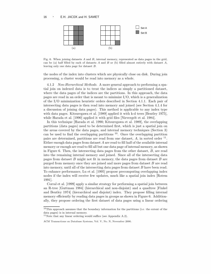
Fig. 6. When joining datasets A and B, internal memory, represented as data pages in the grid,can be (a) half filled by each of datasets A and B or (b) filled almost entirely with dataset A,leaving only one data page for dataset B.
the nodes of the index into clusters which are physically close on disk. During joinprocessing, a cluster would be read into memory as a whole.
4.1.2 Non-Hierarchical Methods. A more general approach to performing a spa-tial join on indexed data is to treat the indices as simply a partitioned dataset,where the data pages of the indices are the partitions. In this approach, the datapages are read in an order that is meant to minimize I/O, which is a generalizationof the I/O minimization heuristic orders described in Section 4.1.1. Each pair ofintersecting data pages is then read into memory and joined (see Section 4.1.4 fora discussion of joining data pages). This method is applicable to any index typewith data pages. Kitsuregawa et al. [1989] applied it with k-d trees [Bentley 1975],while Harada et al. [1990] applied it with grid files [Nievergelt et al. 1984].
In this technique [Harada et al. 1990; Kitsuregawa et al. 1989], the overlappingpartitions (data pages) need to be determined first, which is just a spatial join onthe areas covered by the data pages, and internal memory techniques (Section 3)can be used to find the overlapping partitions 10. Once the overlapping partitionpairs are determined, partitions are read from one dataset, A, in sorted order 11.Either enough data pages from dataset A are read to fill half of the available internalmemory or enough are read to fill all but one data page of internal memory, as shownin Figure 6. Then, the intersecting data pages from the other dataset, B, are readinto the remaining internal memory and joined. Since all of the intersecting datapages from dataset B might not fit in memory, the data pages from dataset B arepurged from memory once they are joined and more pages from dataset B are readinto memory, until all of the intersecting data pages from dataset B have been read.To enhance performance, Lu et al. [1995] propose precomputing overlapping indexnodes if the index will receive few updates, much like a spatial join index [Rotem1991].
Corral et al. [1999] apply a similar strategy for performing a spatial join betweenan R-tree [Guttman 1984] (hierarchical and non-disjoint) and a quadtree [Finkeland Bentley 1974] (hierarchical and disjoint) index. They propose filling internalmemory efficiently by reading data pages in groups as shown in Figure 6. Addition-ally, they propose ordering the first dataset of data pages using a linear ordering
10This approach assumes that the boundary information for the partitions (i.e. the extent of thedata pages) is in internal memory.11Note that any linear ordering would suffice (see Appendix A.2).
ACM Transactions on Database Systems, Vol. V, No. N, November 2006.

Spatial Join Techniques · 17
1410 12 16
ab
14
10
12
16
a
1410 12 16
b
Region of linesintersecting line a.
Right End Point
Left End Point
(a) (b)
Fig. 7. As an example of the transformation to multi-dimensional points in a higher-dimensionalspace, (a) two one-dimensional intervals, a and b, that overlap (b) will be near each other whenmapped to two-dimensional points. Any interval that overlaps interval a will be contained withinthe dotted lines when represented as a point. Furthermore, since the left end point of the intervalis represented by the x-axis, all points will be above the dashed, diagonal line since the left endpoint is always less than or equal to the right end point.
(see Appendix A.2). Even though the two indices are of different types, the methodworks because the data pages of the indices are treated as partitions.
The methods described in this section use heuristics to determine the order ofreading partitions. In a relevant analysis, Neyer and Widmayer [1997] showed thatdetermining the optimal read schedule to minimize the number of disk reads isNP-hard if no restrictions are placed on the partitions. However, if the partitionsdo not share boundaries (that is, they do not have any sides in common), theyshow that the problem is easy to solve. If G is a graph where the vertices representthe MBRs of the index nodes and an edge is placed between all of the intersectingnodes between the two datasets, then the optimal read schedule is the Hamiltonianpath through G, which can be found using an algorithm by Chiba and Nishizeki[1989].
4.1.3 Transform to Multi-Dimensional Points. Unlike points, rectangles haveextent, which complicates spatial join algorithms. For instance, since an object willnot fit neatly into a partition, either the object must be replicated into multiplepartitions or the partitions must overlap, as in an R-tree [Guttman 1984]. Transfor-mation methods avoid this problem by transforming objects into multi-dimensionalpoints in a higher dimensional space, such as used by the grid file index [Nievergeltet al. 1984]. For example, a two-dimensional rectangle can be transformed into apoint in four-dimensional space by using the coordinate values of the center point,half of the width, and half of the height as the four values representing the rectan-gle. Alternatively, the rectangle can be transformed using the coordinate values ofthe opposing corner points of the rectangle as the four values, which is a techniqueknown as the corner transformation.
Song et al. [1999] propose a spatial join for data that is indexed using the cornertransformation method. The indices create a partitioning of the multi-dimensionalpoints, and the method for joining the partitions is similar to the non-hierarchicalspatial join methods (Section 4.1.2), which order the processing of overlapping par-tition pairs between the two datasets. However, in the transformed space, the searchspace substantially increases. For instance, when joining two indexed datasets, R
ACM Transactions on Database Systems, Vol. V, No. N, November 2006.

18 · E.H. JACOX and H. SAMET
Space B
Space A
Space BSpace A
x
x
x
x
Fig. 8. When joining two data pages, only the objects within the intersecting region of the pages(marked with an x) need to be considered.
and S, a region (data page) containing points from a dataset R needs to be com-pared against a larger region containing points from dataset S. To see why this isso, consider the one-dimensional intervals, a and b, shown in Figure 7a. In two-dimensional space, any interval that overlaps a, such as b, will be contained withinthe region shown in Figure 7b, lying between the dashed and dotted lines. Notethat all data points in transformed space are above the diagonal since the termi-nating point of the interval is always greater than the starting point. Similarly, fortwo-dimensional objects, such as a rectangle r (for example, the MBR of an indexnode), all rectangles overlapping r will occupy a space in four dimensions similarto the region shown in Figure 7b (see Song et al. [1999] for the exact calculationof this region in four dimensions). Once the overlapping partition pairs have beendetermined, the methods in Section 4.1.2 can be used to order the reading of thedata pages from memory.
4.1.4 Node to Node Comparison. When joining two regions A and B, whichcould represent two index nodes, two data pages, or two partitions, if both regionscover the same space and fit in internal memory, then every object in region Aneeds to be joined with every other object in region B. This, of course, is aninternal memory spatial join and an appropriate internal memory technique fromSection 3 should be used. For smaller page sizes, a nested-loop join (Appendix A.3)might be best because of the low overhead. For larger page sizes, the plane-sweepmethod (Section 3.1), as suggested by Brinkhoff et al. [1993], or a Z-order sweep(Section 3.2) would be more appropriate.
If the regions do not cover the same space, as is likely when joining index nodes,then the search space can be reduced [Brinkhoff et al. 1993]. Only objects withinthe intersecting region of the two nodes need to be compared, as shown in Figure 8.For example, if the plane sweep method is used to join the nodes, then only theseobjects will be processed by the plane sweep.
4.2 One Dataset Not Indexed
If only one dataset is indexed, then the spatial join can be performed using anindex nested loop join (Appendix A.3), which uses the index to do window queries.For example, given two datasets to be joined, A and B, if dataset A is indexedwith an R-tree, then for every element b in B, a window query is performed on theR-tree index of A using each b, which finds all of the objects in A that intersect
ACM Transactions on Database Systems, Vol. V, No. N, November 2006.

Spatial Join Techniques · 19
A
F
G
ED
B
C
A
B C
D E F G
Seed LevelA
F
G
ED
B
C
p
(a) (b) (c)
Fig. 9. (a) The data (dark rectangles) and regions (lettered squares) covered by the nodes of anR-tree. (b) As shown in a hierarchical representation of the index node structure, the second levelof the R-tree is used as a seed level. (c) Since object p, from the second, unindexed dataset, doesnot overlap any seed level region (regions B and C), p can be discarded.
b. Another approach is to construct an index on the unindexed data and then usethe spatial join techniques for when both datasets are indexed, which are describedin Section 4.1. In support of this approach, techniques for efficiently constructingthe second index are surveyed in Section 4.2.1. Still another approach is to takeadvantage of the structure of the indexed data, without using the index directly,as described in Section 4.2.2, which reviews techniques that partition the leaves ofthe index, and Section 4.2.3, which reviews methods that adapt the plane-sweepalgorithm (Section 3.1) to use the index as a source of sorted data.
4.2.1 Constructing A Second Index. If only one dataset is indexed, then theother dataset can be indexed efficiently using bulk-loading techniques [Hjaltasonand Samet 1999; van den Bercken et al. 1997], which exist for many types of indices,and then the techniques described in Section 4.1 can be used to perform the spatialjoin. This approach is especially useful when the index will be saved and usedlater. Conversely, if the index is not going to be reused, then Lo and Ravishankar[1994] suggest building a special purpose index that improves the performance ofthe spatial join. However, the index might not be reusable because some of thedata will be excluded from the specially built index. This constructed index, whichis an R-tree [Guttman 1984], is built so that it mirrors the structure of the existingindex, thereby minimizing node overlap between the two indices and reducing thenumber of node-to-node comparisons, which speeds the spatial join.
Lo and Ravishankar [1994] call their constructed index a seeded tree since it isbuilt using the upper levels of the existing index to seed the construction of thesecond index. An upper level of the existing index, termed a seed level, is used topartition the second dataset. For efficiency, the level should be chosen such thateach node is assigned a write buffer. The number of write buffers is limited bythe amount of internal memory, which, therefore, determines the lowest level ofthe index that can be used. Lo and Ravishankar discuss techniques for choosinga level in [Lo and Ravishankar 1995]. In a slightly different approach, Mamoulisand Papadias [1999] point out that trying to create too many partitions will causebuffer thrashing and propose a bottom-up approach instead (see Section 4.2.3).One level of the existing index forms a collection of non-disjoint regions that do notnecessarily cover the data space. This is illustrated in Figure 9a and b by regionsB and C. Each region’s centroid, for example, the center points of the MBRs ofthe data pages, serves as the basis for partitioning the second dataset. Initially,
ACM Transactions on Database Systems, Vol. V, No. N, November 2006.

20 · E.H. JACOX and H. SAMET
each partition of the new index has no area. As objects from the unindexed datasetare inserted into a selected partition, the partition is enlarged to enclose all of itsobjects. Lo and Ravishankar experimented with different techniques for choosingthe partition in which to insert objects for the unindexed dataset. The techniquethat performed the best in their experiments is to insert an object into the partitionwith the nearest centroid. Another technique, which performed slightly worse, isto insert the object into the partition whose size is enlarged the least.
Once the data is partitioned, each partition is transformed into an R-tree usingbulk-loading techniques [van den Bercken et al. 1997]. The resulting forest of R-trees is attached to the upper seed levels, which are duplicated from the originalindex, and the new seed levels are adjusted to cover the newly created forest ofR-trees, resulting in a regular R-tree. Once this is done, the techniques given inSection 4.1.1 can be used to perform the spatial join. Since the trees are similar,performance improves because the number of overlapping nodes is reduced. Toimprove performance even further, Papadopoulos et al. [1999] note that duringconstruction of the R-tree, the leaves of the R-tree (or partitions in general) donot need to be written to external memory to form the full external memory indexif the R-tree is not going to be reused. Instead, the leaves or partitions can bejoined to the other dataset immediately and then thrown out, saving I/O cost andspeeding the spatial join.
Lo and Ravishankar [1994] also propose extensions to filter the second dataset,reducing the size of the second dataset and, thus, further speeding the join. Giventwo datasets A and B, where A is indexed and B is not, they note that any object inB, say b, that does not intersect with the regions covered by the upper level nodesof the existing index on dataset A, could not intersect any object in A. Therefore,b does not need to be inserted into the constructed index for dataset B. Thismakes the join faster, but renders the second index unusable for processing otheroperations in the future since it does not contain the entire dataset. For example,if the constructed R-tree is not going to be reused, then objects from the seconddataset that do not intersect the regions covered by the seed levels do not needto be inserted into the partitions because they will not intersect any object in theindexed dataset, as shown in Figure 9c for object p.
4.2.2 An Index as Partitioned Data. Even if just one dataset is indexed, the bestapproach to performing a spatial join might not be to construct a second index,but rather to use the synchronized traversal methods from Section 4.1.1. In thiscase, the pre-existing index can be viewed as a partition of the dataset and methodssimilar to the non-hierarchical methods (Section 4.1.2) can be used to perform thespatial join. To create partitions from an index, the data pages are grouped toform the partitions. The data pages can be grouped either in a top-down mannerfor hierarchical indices by using sub-trees as the partitions [van den Bercken et al.1999] or in a bottom-up fashion by grouping data pages, which can be used for anyindex type [Mamoulis and Papadias 2003].
In a top-down method to partitioning, proposed by van den Bercken et al. [1999],the unindexed dataset is partitioned based on one of the levels of the existinghierarchical index, for example, the sub-nodes of the root of the indexed dataset,which is similar to the seeded tree technique in Section 4.2.1 and shown in Figure 9b.
ACM Transactions on Database Systems, Vol. V, No. N, November 2006.

Spatial Join Techniques · 21
(a) (b)
Fig. 10. (a) A set of index data pages (b) are grouped to form slots, shown by thick-lined rectangles.
The partition boundaries are the MBRs of the internal index nodes for the chosenlevel, for example, regions B and C in Figure 9. The unindexed data is partitionedbased on these regions, placing each object into each partition that it overlaps,which replicates the data, requiring that duplicate removal techniques be used onthe result pairs (see Section 4.3.4).
Once the partitioning is done, each partition is joined with the objects in thesub-tree of the corresponding index node using any appropriate internal memorymethod (Section 3). If the data pages and partitions for a sub-node do not fit inmemory, then the method can be recursively applied by descending to the nextlevel of the index. This approach works best if the depth of the tree is small or,conversely, if the index has a large fan out. For this reason, van den Bercken etal. [1999] propose this approach as a technique for joining two unindexed datasets,in which case an index is created with the largest possible fan out on one datasetbefore the method is applied.
In a bottom-up approach to partitioning the data pages, Mamoulis and Papa-dias [1999; 2003] propose a technique that creates a target number of partitions,which they call slots, by grouping the data pages of the existing index, as shown inFigure 10. The unindexed dataset is partitioned based on the slots. To create theslots, the amount of data in each slot is first determined, which is roughly half ofthe available internal memory. The data pages of the existing index are grouped bytraversing them in a linear order (Appendix A.2) and adding them to a slot untilthe slot’s capacity is reached. Then, the next slot is filled and so forth. The regioncovered by the data pages in the slot form a partition for the unindexed data. Aswith the top-down approach, once the unindexed dataset is partitioned, a group ofdata pages from the original index (a slot) and its corresponding partition of theunindexed dataset are read into memory and joined. Due to skew, however, a slotand its partition might not fit in internal memory. In this case, the partitioningmethod is applied recursively until each slot and its partition fit in memory.
4.2.3 An Index as Sorted Data. An index can also be viewed as a sorted dataset,since extracting the data from an index in sorted order is inexpensive using an in-order traversal of the index. In this case, the plane-sweep method (Section 3.1) canused to perform the spatial join. Generally, the plane-sweep method is performedafter sorting both datasets. Since extracting data from an index in sorted order(sorted in one-dimension) is fast in this situation, the plane-sweep technique is lessexpensive than sorting both datasets since only one dataset needs to be sorted [Argeet al. 2000].
ACM Transactions on Database Systems, Vol. V, No. N, November 2006.

22 · E.H. JACOX and H. SAMET
Fig. 11. The leaves of an R-tree are grouped into strips, which can flushed to external memoryif internal memory overflows. Here, four strips (dashed lines) are formed, each containing twoobjects.
Another approach, one that modifies the plane-sweep method, proposed by Gur-ret and Rigaux [2000], is to read the data pages from an index (they use an R-tree)in a one-dimensional sorted order and insert entire data pages into the sweep struc-ture. In this case, one sweep structure will contain objects, as is normal, whilethe other sweep structure will contain data pages. This technique only requiresa modification of the plane-sweep SEARCH routine (see Figure 2) to search for in-tersections between an object and a data page. Since the REMOVE INACTIVE andINSERT routines work with MBRs and the enclosing rectangle of a data page is anMBR, these two methods do not need to be modified. Additionally, the initial sortstep of the plane-sweep algorithm needs to extract the data pages of the index aswell as to sort the unindexed dataset.
If memory overflows (that is, the active set is too large to fit in internal memory),then Gurret and Rigaux [2000] propose using a method in which some of the datapages of the index are removed (or flushed) from the sweep structure and written todisk for later processing. To do this, before the plane-sweep phase of the algorithmstarts, each data page is assigned to a strip, as shown in Figure 11. The stripsare created using a method that is similar to forming slots in Section 4.2.2, exceptthat a one-dimensional sort is used. Only entire strips of data pages are flushedat a time. After a strip is flushed, the plane-sweep algorithm continues. Anyrectangle from the unindexed dataset that overlaps the flushed strip is also writtento external memory. After the plane-sweep algorithm finishes, it is run again on theflushed data pages and the rectangles written to external memory, starting from thepoint where the flush occurred. If a plane sweep on the flushed data also overflowsmemory, then the flushed data can be partitioned further into strips and the entirealgorithm applied recursively.
4.3 Neither Dataset Indexed
The inputs to a spatial join operation are usually assumed to be indexed. However,the situation is often different when the input to the spatial join are themselves theresult of a spatial join. In particular, there is no requirement that the output of aspatial join be indexed (but see Hoel and Samet [1995], which evaluates differentspatial indices by taking into account the time necessary to construct an index forthe result of a spatial join). If neither dataset is indexed, then an index can bebuilt on one or both datasets, and then the techniques from Sections 4.1 and 4.2,respectively, can be used. If the index is to be saved and reused, this can make
ACM Transactions on Database Systems, Vol. V, No. N, November 2006.

Spatial Join Techniques · 23
1 2
3 4
Set A
Set B
1 2
3 4
Fig. 12. If both datasets, A and B, are partitioned using the same grid, then each grid cell isjoined with exactly one other, corresponding cell.
sense. If not, then other techniques that do not necessarily create an index mightbe faster 12. These techniques are useful when an index would not be used later,such as for a one-time operation on the data, where the extra cost of building theindex would be more expensive. For example, in a complex query, intermediateresults can be processed faster with these techniques. The key to most of thesetechniques lies in partitioning the datasets so that the partitions are small enoughto fit in internal memory. In other words, a divide-and-conquer approach is usedto decompose the datasets into manageable pieces.
Once the data is partitioned, each pair of overlapping partitions, one from eachdataset, is read into internal memory and internal memory techniques are used (seeSection 3). This assumes that the partition pairs fit into internal memory. If theydo not, then they can be repartitioned until the pairs fit (see Section 4.3.3).
As a foundation for describing the partitioning methods in this section, Sec-tion 4.3.1 describes a generic algorithm for performing a spatial join using a par-titioning technique. The algorithm also serves to introduce several common issuesassociated with the partitioning approach: determining the number of partitionsis discussed in Section 4.3.2, repartitioning, if any of the partition pairs do not fitin internal memory, is discussed in Section 4.3.3, and handling duplicate results isdiscussed in Section 4.3.4.
Details of specific methods are found in Appendix B. Appendix B.1 discussesan extension to the plane-sweep algorithm (Section 3.1) that can process datasetsof any size by using external memory. The distinction between the sort-and-sweepmethod and the partitioning method is analogous to the distinction between sort-merge joins and hash-based joins. Next more sophisticated partitioning algorithmsfrom the literature are described, grouped by how they partition the data: usinggrids in Appendix B.2, using strips in Appendix B.3, by size in Appendix B.4, andclustering in Appendix B.5.
4.3.1 Basic Partitioning Algorithm. This section uses a simplified algorithm toillustrate a spatial join technique based on partitioning. While the algorithm haslimited practical applications, it is used as the basis for describing more sophis-ticated algorithms and to discuss the common issues associated with partitioningtechniques. The basic concept is to define a grid and use it to partition the datafrom each dataset, datasets A and B, into external memory. Each data object isplaced into each grid cell (partition) that it overlaps. Once the data is partitioned,
12Some techniques for unindexed data create a usable index as a byproduct of the spatial join,for example, the filter tree [Koudas and Sevcik 1997].
ACM Transactions on Database Systems, Vol. V, No. N, November 2006.

24 · E.H. JACOX and H. SAMET
1 procedure GRID JOIN(setA, setB)
2 begin
3 /* determine the number of partitions */
4 m←AVAILABLE INTERNAL MEMORY;
5 mbrSize←BYTES TO STORE MBR;
6 minNumberOfPartitions←(SIZE(setA)+SIZE(setB))*mbrSize/m;
7 partitionList←DETERMINE PARTITIONS(minNumberOfPartitions,
8 AREA OF DATA SPACE);
9 /* partition data to external memory */
10 partitionPointersA←PARTITION DATA(partitionList, setA);
11 partitionPointersB←PARTITION DATA(partitionList, setB);
12 /* join partitions */
13 foreach partition ∈ partitionList do
14 partitionA←READ PARTITION(partitionPointersA, partition);
15 partitionB←READ PARTITION(partitionPointersB, partition);
16 PLANE SWEEP(partitionA, partitionB);
17 enddo;
18 end;
Fig. 13. A simple partitioning technique for performing a spatial join on unindexed data.
the partitions for each grid cell of dataset A are joined with the corresponding par-tition of dataset B using one of the internal memory methods from Section 3. Forexample, in Figure 12, both datasets A and B are partitioned using the same grid,and then, each corresponding cell is joined with the other. Grid cell 1 from datasetA, for instance, is joined with cell 1 from dataset B, and so forth.
In the algorithm, shown in Figure 13, the first step is to determine how manypartitions are needed. The goal is to create partitions that are small enough, whenpaired with a corresponding partition, to fit in internal memory. To do this, thealgorithm first calculates the minimum number of partitions needed, minNumberOf-Partitions, as the total storage costs of the objects in both datasets divided by theavailable internal memory. The algorithm uses the DETERMINE PARTITIONS functionto create the smallest grid that has at least minNumberOfPartitions. However,the calculation of minNumberOfPartitions is inaccurate for two reasons. First,if a dataset is skewed, then some grid cells might contain more objects than canfit in internal memory. The more sophisticated techniques described later in thissection correspond to different ways of dealing with skewed data. The simplifiedalgorithm assumes that the data is uniform. Second, since a data object is placedinto each cell it overlaps, the number of data objects will increase since the objectis replicated into each cell. To address this issue, the calculation of the minimumnumber of partitions can be adjusted using methods described in Section 4.3.2.Alternatively, the algorithm can continue and when a partition pair to be joined isencountered that is too large for internal memory, then one or both of the partitionscan be repartitioned, creating smaller partitions that can be processed. Section 4.3.3addresses repartitioning. Note that since objects are replicated into multiple cellsfor both datasets, duplicate results will arise. Section 4.3.4 addresses the issue ofremoving duplicates from the result dataset.
Once the partitions are created, the algorithm scans the datasets, placing eachobject into each partition that it overlaps using the PARTITION DATA function, whichwrites the objects to external memory. In the final step of the algorithm, each
ACM Transactions on Database Systems, Vol. V, No. N, November 2006.

Spatial Join Techniques · 25
partition pair is read into internal memory using the READ PARTITION function andjoined using the plane-sweep technique from Section 3.1 (note that any internalmemory spatial join would be appropriate), which will report all of the intersectingpairs between the partitions.
4.3.2 Determining the number of partitions. Many partitioning techniques mustfirst determine a target number of partitions. The goal is to create pairs of partitionto be joined that will fit in memory. However, because of data skew, no simplepartitioning scheme can guarantee that all of the partition pairs will fit in memory.Therefore, a heuristic calculation must be used. This calculation is constrained bythe following factors:
(1) The amount of internal memory, which determines the number of objects thatcan be joined at a time using internal memory techniques.
(2) The replication rate, which is the actual number of objects inserted into thepartitions, which includes duplicates.
(3) The amount of internal memory also limits the number of write buffers thatcan be used to partition the data to external memory.
Within these constraints, different techniques either try to maximize or minimizethe number of partitions. A minimum number of partitions might be calculatedin order to reduce replication, which reduces the number of pairs that need tobe joined. A maximum number of partitions minimizes the chances of a costlyrepartitioning.
The simplest calculation, ignoring data skew and replication, derives the tar-get number of partitions by dividing the total storage costs of the objects by theavailable internal memory. The total storage costs of the objects is the number ofobjects multiplied by the size of an object in bytes, referred to as objectSize. In animplementation, objectSize might be the sum of the size of a rectangle (MBR) inbytes and the size of an object pointer or object key. To account for replication, ascale factor, r, can be added to the calculation. The replication rate depends on thedataset and the partitioning scheme. In one set of experiments [Patel and DeWitt1996], the replication rate was found to be 3-10%. Incorporating the replicationscale factor, r, the calculation for the minimum number of initial partitions is:
r · (|setA| + |setB|) · objectSize
m, (1)
where m is the available internal memory. However, this equation does not takeinto account data skew and is only an estimate. In the worst case, with severelyskewed data, most of the data could be in one partition. In this case, repartitioningis required (see Section 4.3.3).
Equation 1 applies to internal memory methods that require all of the data to beread into internal memory before processing begins. Arge et al. [1998] showed thatthe plane-sweep method can process more data than can fit into internal memory,see Section 3.1. However, the exact amount of data that can be processed is de-pendent on the dataset, specifically the maximum density of the dataset [Faloutsosand Kamel 1994; Jacox and Samet 2003; Theodoridis et al. 1998], which is just themaximum number of objects in the active set. However, this value is difficult tocalculate for a given dataset.
ACM Transactions on Database Systems, Vol. V, No. N, November 2006.

26 · E.H. JACOX and H. SAMET
The maximum number of partitions is limited by internal memory in that internalmemory limits the number of external memory write buffers. Typically, for betterperformance, when writing to external memory, a page of internal memory is filledbefore it is flushed to external memory. This places a hard limit on the maximumnumber of partitions.
The principal motivation for getting the number of partitions right is to avoidrepartitioning (see Section 4.3.3). However, the more partitions there are, thegreater the replication. Some evidence suggests that this replication does not havea significant impact on the total processing time [Zhou et al. 1997]. In this case,creating the maximum number of partitions might optimize performance. Con-versely, internal memory algorithms might perform better with smaller partitions,thereby improving overall performance. From the literature, it is unclear what thebest choice is for the number of partitions and thus, we leave this choice as an openquestion.
4.3.3 Repartitioning. The goal of partitioning is to create partitions that aresmall enough to be processed by internal memory techniques (Section 3). However,the initial partitioning phase (Section 4.3.2) might create partitions that are toolarge because of data replication or skewed data. If this occurs, then the partitionpairs that are too large can be further sub-divided using the original partitioningscheme, creating a finer grid. If this repartitioning fails, then the process can berepeated recursively until all of the partition pairs can be processed by internalmemory methods.
Repartitioning can occur immediately after the initial partitioning, or it mightbe necessary to do it later, after some partition pairs have been joined because itmight not be known if a repartitioning will be necessary. With the basic internalmemory techniques, such as the nested-loop join (Section 3), the size of the datasetsthat can be processed is known, in which case, any over-full partition pairs can berepartitioned immediately, before joining any of the partitions. However, with otherinternal memory techniques, such as the plane-sweep extension [Arge et al. 1998],it might not be known whether or not a partition pair is small enough. In this case,repartitioning is done only when an internal memory technique fails because itssweep structure has grown too large for the available internal memory. Any resultpairs generated for the current partition pair need to be discarded since the resultswill be regenerated after repartitioning.
If a partition pair to be joined, say A and B, is too large for the available internalmemory, Dittrich and Seeger [2000] propose repartitioning only one of the datasets,say A, first, and then joining each sub-partition with B. If this fails to create smallenough partitions, then the other dataset, B can be repartitioned. This processcan also occur recursively until small enough partitions are achieved.
4.3.4 Avoiding Duplicate Results. If partitioning the data results in object repli-cation, then duplicate results will be reported. For instance, if a pair of overlappingobjects is split by a partition boundary, then the intersecting pair will be reportedwhen each partition is processed, as shown in Figure 14a. Some experiments haveshown that replication does not add considerably to processing [Zhou et al. 1997],though other experiments have shown the opposite [Luo et al. 2002]. In either case,
ACM Transactions on Database Systems, Vol. V, No. N, November 2006.

Spatial Join Techniques · 27
ab
Partition Boundary
x
Partition A
Partition B
(a) (b)
Fig. 14. (a) An intersection between objects a and b is reported from both partitions into whichthey are inserted, creating a duplicate result. (b) The reference point method for online duplicateavoidance only reports an intersecting pair if a point in the intersecting region, x, is within thecurrent partition. The point must be chosen consistently, such as always the lower left corner.
duplicate results need to be removed from the candidate set to avoid extra pro-cessing during the refinement stage (Appendix D). The duplicates can be removedwith an extra step between the filtering stage and the refinement stage or combinedwith refinement. With some algorithms, duplicate results can be detected duringfiltering and removed online.
One way to remove duplicate results from the candidate set after the filteringstage is to sort the candidate set and then scan the sorted list, removing duplicates.Some refinement techniques sort the candidate set first, and thus, this duplicateremoval technique can be used without a loss of performance (see Appendix D).However, to sort the candidate set, the entire candidate set must be producedfirst. In most database systems, that is, demand-driven pipelined systems [Graefe1993], results need to be produced continuously. In this case, online duplicate
removal techniques, which remove duplicates as they appear in the filtering stage,are preferred.
To implement online duplicate removal, the internal memory spatial join tech-niques (Section 3) can be modified with a simple test which is applied when therectangles are checked for intersection. The technique, termed the reference point
method [Aref and Samet 1994b; Dittrich and Seeger 2000; Seeger 1991], calculatesa point within the intersecting region of the two objects. The pair is reported onlyif this point is within the current partition. The test point can lie anywhere withinthe intersecting region of the two objects, such as the centroid of the region or acorner point, but must be chosen consistently 13. For instance, as shown in Fig-ure 14b, reference point x is the lower left corner point of the intersecting region ofthe two rectangles. Since point x only lies within the B partition, the intersectingrectangles will only be reported when the B partition is processed, but not whenthe A partition is processed, even though the A partition also includes the rectanglepair.
5. SPECIALIZED SPATIAL JOINS
A basic spatial join is executed between two sets of objects on the same machinewith a single processor. Modifications of the spatial join can be made to improveperformance when more than two sets of objects are joined in a multiway join,as described in Section 5.1. Also, the spatial join requires special considerations
13To use the reference point method, the approximations of the objects cannot be clipped, thatis, the full MBR must be stored and not just the portion of the object within a partition (mostpartitioning methods don’t use clipping).
ACM Transactions on Database Systems, Vol. V, No. N, November 2006.

28 · E.H. JACOX and H. SAMET
b
a
cb
a
c
ba c
(a) (b) (c)
Fig. 15. Three objects with (a) mutual intersection, (b) pair-wise intersection, (c) two of theobjects not intersecting.
A
B
C D
E
F G
Fig. 16. A graph representing the relations between datasets in a complex query between multipledatasets. Each edge is a join condition between the objects, which might be more than a binaryrelation, such as the ternary relation joining A, B, and C.
when it is performed using a parallel architecture, described in Section 5.2, or ondistributed computers, described in Section 5.3.
5.1 Multiway Joins
A complex query could contain multiple spatial joins. As an example, consider thequery – find all regions between 500 meters and 700 meters above sea level that re-
ceive 10 to 15 centimeters of rainfall and are in a forested area. This query requiresa spatial join to find the intersecting regions of rainfall and elevation and also theintersection with land type (forest). This query can be answered by performing aspatial join between any two of the datasets and joining the results with the thirddataset. The intermediate results are the intersecting regions of the result candi-date set, which is then joined with the third dataset. In the example, rainfall andelevation can be joined, creating a new dataset that represents regions with 10 to 15centimeters of rainfall and which are between 500 and 700 meters above sea level.This intermediate dataset is then joined with the land type data to create the finalresult.
The previous example illustrates a query with mutual intersection between thedatasets. A spatial query might not require that the datasets mutually intersect.For example, the query – find all roads that cross a river and a railroad track –does not require that the river and the railroad track in a result triplet intersect. InFigure 15a, the three objects have a mutually intersecting region, but in Figure 15b,each object pair-wise intersects. Furthermore, it is not necessarily the case that arelationship exists between all of the datasets in the query. For instance, as shownin Figure 15c, the query could only require that objects from dataset B intersect anobject from both A and C, but no restriction is placed on intersections between Aand C, such as with the road, river, and railroad example. In general, a multiwayspatial query can be represented by a graph, as shown in Figure 16, in which n-
ACM Transactions on Database Systems, Vol. V, No. N, November 2006.

Spatial Join Techniques · 29
1 procedure MULTI INDEX NLJ(joinCondition, setA, setB, setC)
2 begin
3 spatialIndexB←CREATE SPATIAL INDEX(setB);
4 spatialIndexC←CREATE SPATIAL INDEX(setC);
5 foreach a ∈ setA do
6 tempSetB = spatialIndexB.SEARCH(a);
7 foreach b ∈ tempSetB do
8 tempSetC = spatialIndexC.SEARCH(b);
9 foreach c ∈ tempSetC do
10 if SATISFIED(a, b, c, joinCondition) then
11 REPORT(a, b, c);
12 endif;
13 enddo;
14 enddo;
15 enddo;
16 end;
Fig. 17. A multiway index nested loop join that finds objects from three datasets that satisfy anytype of multiway intersection (see Figure 15).
ary relations are used to represent mutually intersecting regions. For instance,in Figure 16, objects from A, B, and C are required to mutually intersect, as inFigure 15a, as opposed to objects D, F , and G, which are only required to pair-wiseintersect, as in Figure 15b.
As mentioned, a multiway spatial join can be solved by joining two datasetsat a time and creating intermediate datasets. Furthermore, traditional databaseoptimization approaches [Graefe 1993] that order the pair-wise joins to efficientlysolve the query can be used [Mamoulis and Papadias 1999]. To do this, selectivityestimates (Section 6) are required in order to efficiently determine which pair ofdatasets to process first, typically processing the pair that produces the smallestintermediate result set first. Moreover, query optimizers also need selectivity in-formation in order to efficiently perform queries that involve a mix of spatial andaspatial data.
To be more efficient, several techniques have been proposed for extending thefiltering algorithms (Sections 3 and 4) to process multiple datasets at once. Forexample, the nested-loop join (Appendix A.3) can be extended to process threedatasets simultaneously by nesting another loop and using a join condition thattakes three arguments, which tests for a three-way intersection. Section 5.1.1 de-scribes a similar extension to the index nested-loop join (Appendix A.3), whichserves as a basis for describing a more sophisticated technique that is derived fromconstraint satisfaction problem (CSP) techniques [Kumar 1992]. Next, Section 5.1.2describes extending the synchronized traversal spatial join (Section 4.1.1) to per-form a multiway spatial join.
5.1.1 Multiway Indexed Nested-Loop Spatial Joins. A multiway version of theindex nested loop algorithm (Appendix A.3) can be created by nesting each addi-tional dataset. This algorithm, shown in Figure 17, is a simplification of algorithmsby Mamoulis and Papadias [1998] and Papadias et al. [1998], and only joins threedatasets. More datasets could be joined with further nesting, but the temporarycandidate sets can grow significantly larger with more datasets. A generic join
ACM Transactions on Database Systems, Vol. V, No. N, November 2006.

30 · E.H. JACOX and H. SAMET
condition, termed joinCondition, that specifies the desired relation between thedatasets, is used since a relation other than intersection might be required. How-ever, each dataset is assumed to be involved in some form of an intersection relationwith another dataset. Otherwise, the multiway spatial join might not be appropri-ate.
The first step in the algorithm, shown in Figure 17, indexes setB and setC.Then, for each element of setA, a window query is performed on the index ofsetB using the SEARCH method. This assumes that the relation specifies that setAand setB intersect. Each of the search results from setB is used to perform awindow query on setC, which produces another intermediate result set. Note thatnot all elements of setC need to intersect elements of setA as intersection is nota transitive relation (for example, objects a and c in Figure 15c do not intersecteach other, even though they both intersect object b). Finally, each result fromsetC, along with the current value for setA and setB are checked to ensure thatthey satisfy the given relation using the SATISFIED function, and if so, the valuesare reported. The SATISFIED function ensures that the specified join condition ismet. For example, if mutual intersection is required, as in Figure 15a, then theintersections of the type shown in Figures 15b and c will not be reported. Notethat the algorithm explicitly instantiates the temporary result sets, for example,tempSetB. This is done in order to give the reader an idea of the internal memoryrequirements of the algorithm. A database iterator could be used instead, therebyletting the database engine optimize storage and retrieval of the temporary resultset.
To enhance the performance of the algorithm, if the query seeks mutually inter-secting rectangles, each search can use the intersections of the current values of theprevious datasets to further improve performance. For instance, when the index onsetC is searched, the intersection of a and b would be the search window, ratherthan just b. Papadias et al. [1998] refer to this approach as a window reduction. Ina hybrid approach, Papadias et al. [1998] propose performing a normal spatial joinon two of the datasets first, which should be faster than a nested-loop join, andthen using window reduction for the remaining values.
To enhance the performance of the algorithm further, each temporary resultset could be checked against all previous relations to further prune the result set.For example, the algorithm only considers the relations between setA/setB andsetB/setC. A relation could exist between setA and setC, as in Figure 15a. Ifmore datasets were being joined with further nesting, then reducing the size oftempSetC would be advantageous. In this case, after the temporary result set forsetC is generated (tempSetC), it could be checked against the current value fromsetA, a, to further reduce the size of tempSetC.
The previous enhancement can be carried even further by having each currentset immediately prune each following dataset. For instance, in the algorithm inFigure 17, each value from setA could be used to produce temporary sets for everyother dataset, setB and setC, before scanning any other dataset. Papadias etal. [1998] and Mamoulis and Papadias [1998; 2001a] use this approach to solve themultiway spatial join, which is a constraint satisfaction problem (CSP) technique[Kumar 1992] called multi-level forward checking. In the CSP approach, temporary
ACM Transactions on Database Systems, Vol. V, No. N, November 2006.

Spatial Join Techniques · 31
1 procedure MULTI INDEX CSP(joinCondition, setA, setB, setC)
2 begin
3 tempSetA←∅
4 tempSetB←∅
5 foreach a ∈ setA do
6 foreach b ∈ setB do
7 if SATISFIED(a, b, joinCondtion) then
8 tempSetB←tempSetB ∪ b
9 endif;
10 enddo;
11 if relation between setA and setC then
12 foreach c ∈ setC do
13 if SATISFIED(a, c, joinCondtion) then
14 tempSetC←tempSetC ∪ c
15 endif;
16 enddo;
17 else
18 tempSetC = setC;
19 endif;
20 /* inner loop */
21 foreach b ∈ tempSetB do
22 foreach c ∈ tempSetC do
23 if SATISFIED(a, b, c, joinCondtion) then
24 REPORT(a, b, c);
25 endif;
26 enddo;
27 enddo;
28 enddo;
29 end;
Fig. 18. A multiway index nested loop join that finds objects from three datasets that satisfy anytype of multiway intersection using constraint satisfaction problem (CSP) techniques to prunetemporary datasets.
result sets are generated as soon as possible. In this algorithm, shown in Figure 18,if a relation exists between setA and setC, then a temporary result set, tempSetC,is generated in the outer loop using the current value from setA. If a relation existsbetween each dataset, then all temporary results are generated in the outer loopwith each object from setA. These sets are pruned as each object is instantiatedfor each dataset in the nested loops. As a further possible enhancement, anotherCSP technique is to dynamically vary the order in which the datasets are processed,choosing the one with the smallest temporary result set first.
5.1.2 Multiway Hierarchical Traversal. Papadias et al. [1998] and Mamoulis andPapadias [1998; 2001a] extend the hierarchical traversal method (Section 4.1.1) todo a multiway spatial join. This technique applies if each dataset is indexed using ahierarchical index, such as an R-tree [Guttman 1984]. For two datasets, the originalmethod compares overlapping nodes of the two indices. If the nodes are leaves, theintersecting objects within the node are reported, else the intersecting child nodepairs are placed on a priority queue to be processed later. To do a multiway join,the queue is modified to hold multiple nodes, one from each dataset, instead ofpairs. To start, the root nodes of the indices are checked and combinations of
ACM Transactions on Database Systems, Vol. V, No. N, November 2006.

32 · E.H. JACOX and H. SAMET
Index Node a1
Index Node b1 Index Node b2
Fig. 19. Objects in multiple partitions might be read from memory multiple times.
the root node’s children that satisfy the join condition are placed on the queue.Next, the first set of nodes on the queue is checked and combinations of childrenare put on the queue. This process repeats until the queue is empty. Papadiaset al. [1998] and Mamoulis and Papadias [1998] suggest using multi-level forwardchecking (Section 5.1.1) to check the nodes, but any appropriate multiway versionof an internal memory spatial join could be used. For instance, Park et al. [1999]propose using a pair-wise plane-sweep method for comparing multiple nodes atonce, that is, a plane-sweep method is used on the first two datasets and the resultsare joined with the third dataset with the plane-sweep method, and so forth. Asan alternate hybrid approach, Papadias et al. [1999] propose using the hierarchicaltraversal approach to instantiate the first few variables, then finishing with windowreduction (Section 5.1.1) to instantiate the remaining variables.
5.2 Parallel
In a parallel architecture, work is distributed amongst several processors. For aspatial join, the work can be distributed in both the filtering and refinement stages,and also for partitioning unindexed data. For the filtering stage, parallel techniquesthat extend the synchronized hierarchical traversal approach (Section 4.1.1) havebeen used for indexed data [Brinkhoff et al. 1996], and techniques that extend thegrid partitioning methods (Appendix B.2) have been used for unindexed data [Luoet al. 2002; Patel and DeWitt 2000; Zhou et al. 1997]. These techniques assume ashared nothing architecture (each processor has it’s own memory), although somealgorithms have extensions that use shared memory architectures to improve perfor-mance [Brinkhoff et al. 1996; Zhou et al. 1997]. Most of these methods have showna near linear speed increase with more processors. However, the key to achievinglinear speed increases during filtering depends on load balancing. An algorithmthat uses a specialized hypercube architecture to join two indexed datasets is alsodiscussed [Hoel and Samet 1994].
Brinkhoff et al. [1996] investigated extending the synchronized hierarchical traver-sal approach (Section 4.1.1) to parallel architectures by assigning sub-trees of theindex to each processor. In the simplest approach to distributing the work amongstn processors, a single processor first performs a hierarchical traversal, one level at atime, until the number of node pairs on the priority queue exceeds n. At that time,the node pairs are distributed to the processors, which perform a sequential spatialjoin. However, as shown in Figure 19, one processor might be assigned nodes a1and b1 and another processor the node pair a1 and b2. In this case, node a1 willbe read from memory twice. To overcome this inefficiency, Brinkhoff et al. proposeusing global buffers (in a shared memory architecture) so that one processor canaccess a node that another processor has read into internal memory. However, this
ACM Transactions on Database Systems, Vol. V, No. N, November 2006.
Spatial Join Techniques · 33
approach does incur extra communication costs to synchronize usage of the buffers.Additionally, the workloads might not be balanced since the processing time foreach sub-tree could be different. Rather than assigning all of the node pairs fromthe queue at once, Brinkhoff et al. suggest assigning only one node pair at a time toeach processor. Once a processor finishes with one node pair, another is requestedwhile the queue is not empty. When the queue is empty, they further suggest thatone processor can share the work of another processor by taking node pairs fromanother processor’s local queue, i.e., sub-trees of the original sub-trees.
For unindexed data, Zhou et al. [1997] adapt the variation of the grid partitioningmethod (Appendix B.2) that physically creates the grid cells. In their approach,the random data is evenly divided amongst the n processors, which then partitionthe data using the same tiling scheme. Then, with the sizes of the grid cells known,a single processor determines the merging of grid cells into n partitions using aZ-order merge, creating, on average, an even load distribution amongst the pro-cessors. Next, each processor is assigned a partition and the data is redistributedappropriately. Finally, each processor filters the data using a sequential spatialjoin filtering technique. Both Patel and Dewitt [2000] and Luo et al. [2002] inves-tigated a similar approach. Rather than physically tiling the data, though, theyboth use the virtual tiling method (Appendix B.2), relying on a good hash functionto distribute the data evenly.
For parallel refinement, each processor could refine the candidate pairs it pro-duces. However, Zhou et al. [1997] point out that it is difficult without muchselectivity information to balance the number of candidates produced by each pro-cessor during the filtering stage. If the candidate pairs are redistributed, then theworkload for refinement can be close to optimal since the number of vertices ineach polygon are good estimates of performance. Like sequential refinement, per-formance can be improved by ordering the candidate set to minimize the numberof times each full object is read. Zhou et al. argue that an efficient approach isto use one processor to sort the candidates into a linear order, and then assignthe candidates to each processor in a round-robin fashion. Each processor will beprocessing candidate pairs that are near each other (exhibiting locality), increas-ing the likelihood that an object only needs to be read into internal memory once(assuming a shared memory architecture), rather than continually reading some ofthe same objects throughout refinement. Zhou et al. took the approach of assigningfull objects to processors, which are responsible for reading the object into memoryand distributing the object to other processors. They found that the redistributioncosts are negligible.
Hoel and Samet [1994] describe parallel algorithms for PMR bucket quadtrees[Nelson and Samet 1987] and R-trees [Guttman 1984] using a specialized hypercubearchitecture. The algorithms require that the data fit in memory, but result in ex-tremely fast algorithms. In their quadtree approach, regions of one of the quadtreesare associated with half of the nodes (processors), termed the source nodes, andcorresponding regions of the other quadtree are associated with the other nodes,termed the target nodes. Each quadtree is assumed to cover the same area, andthus, because of the regular decomposition, there is a one-to-one correspondencebetween source nodes and target nodes. The source nodes send their objects to
ACM Transactions on Database Systems, Vol. V, No. N, November 2006.

34 · E.H. JACOX and H. SAMET
the target nodes, which check for intersections. Hoel and Samet also describe asimilar algorithm for R-trees in which the index nodes of the R-tree are associatedwith the processor nodes. However, because of the irregular decomposition, eachsource node will be associated with multiple target nodes, dramatically increasingthe communication costs and slowing the join.
5.3 Distributed
In a distributed spatial join, the datasets reside at different locations. Abel etal. [1995] show how to combine the semi-join [Mishra and Eich 1992] concept fordistributed join processing and the filter-and-refine approach for spatial join pro-cessing. Given two sets of objects, R and S, that are at different locations (physi-cally distributed), they send the MBRs of dataset R to the S location and filter theobjects there. Then, they send the full objects from S that are in the candidateset to R’s location to perform the refinement step. Tan et al. [2000] point out thatunlike a relational semi-join [Ozsu and Valduriez 1999], where the transmission costis dominant, the processing cost can be just as large of a factor for spatial joins.
Mamoulis et al. [2003] explore the distributed spatial join problem in which thedata resides on different servers between which there is no communication and theservers will not perform a spatial join. This would be the case if the servers arecommercially owned and contain proprietary data. Additionally, it is assumed thatthe servers will not provide statistics on the data. In this case, the spatial join mustbe performed at a third, possibly small, site, such as a mobile device. They pointout that any processing at the data server sites is relatively inexpensive comparedto a mobile device. Therefore, as much work as possible should be done on the dataservers, such as running queries to build useful statistics on the data. To do thespatial join, they propose a grid-based partitioning spatial join (Appendix B.2) anduse the detailed statistics to determine the best grid such that data fits within theavailable internal memory. The statistics are also used to identify empty regionsin a dataset for which no spatial join needs to be performed, thus saving valuabletransmission costs.
6. SELECTIVITY ESTIMATION
Techniques for estimating the selectivity of a spatial join are important as an aidfor analyzing spatial join algorithms, for use in query optimizers, and as a datamining tool. Gunther et al. [1998] have shown that along with the size of thedataset, selectivity is crucial in determining the performance of an algorithm. Queryoptimizers assist a database engine in determining the order of operations in acomplex query. Also, selectivity estimates could play a roll in determining whichspatial join algorithm to use. For instance, a very dense dataset in which nearlyevery pair is reported, could be computed faster using the simple nested loop join(Appendix A.3), rather than a more complex algorithm with a large overhead. Fordata mining applications, selectivity estimates can give approximate answers toqueries, which can be used to rule out hypotheses [Belussi and Faloutsos 1995].
For uniform datasets in two dimensions, a rudimentary estimate of the selectivityfor the filtering stage of a spatial join can be derived from the probability that twoaverage sized rectangles overlap [Aref and Samet 1994a]. Given that both datasetsare enclosed in a universe of finite area, which is represented as TotalArea, the
ACM Transactions on Database Systems, Vol. V, No. N, November 2006.

Spatial Join Techniques · 35
probability that two rectangles with widths wa and wb and heights ha and hb
intersect is:
(wa + wb) · (ha + hb)
TotalArea=
areaa + areab + (wa · hb) + (wb · ha)
TotalArea, (2)
where areaa and areab are the areas of two rectangles 14. To derive a selectivityestimate for a spatial join between two uniform datasets, the average sizes of therectangles in the two datasets A and B are substituted into Equation 2. In thiscase, the selectivity is approximately:
areaA + areab + (wA · hB) + (wB · hA)
TotalArea. (3)
However, the situation is more complicated for non-uniform datasets. Mamoulisand Papadias [2001b], An et al. [2001], and Belussi et al. [2004] propose using a two-dimensional histogram on each dataset, which can be a grid with occupancy counts.Within each grid cell, the selectivity estimate for uniform datasets, Equation 3, canbe applied. The results for each cell are then combined to get an overall estimateof selectivity. The finer the histogram, the more accurate the results will be. An etal. also studied sampling techniques and proposed a novel technique for estimatingintersections within a grid cell by counting the number of sides and corners ofrectangles within each grid cell.
Das et al. [2004] present a method that provides a selectivity estimate of a spatialjoin for skewed datasets. The method requires one scan of the dataset, and has aprovable, adjustable error bound. Each object in the dataset is represented by afixed set of objects from a dyadic cover, with a total size O(log(n)), where n is thesize of the dataset. As each object, r, is encountered, summary statistics for eachdyadic object composing r are updated. By combining these statistics in a mannerthat does not count particular intersections more than once, the method estimatesthe selectivity of the spatial join.
In another approach, working with point datasets, Belussi and Faloutsos [1995]expressed the selectivity of a self-spatial join in terms of a fractal dimension. Sincethe data is points, the spatial join finds all pairs of points within a distance ǫ, whichis expressed as nb(ǫ), and is analogous to the average number of intersecting pairs,that is, the selectivity of the spatial join 15. The average number of nearby, orneighboring, points captures information about the distribution of the data. If thedata is clustered, then the average number of neighbors increases. The problem,then, is to find a good estimate of the number of neighbors. To do so, Belussi andFaloutsos use the fractal correlation dimension D2, which is a characteristic of thedataset, and calculate the average number of neighbors as:
nb(ǫ) = (n − 1) · (2 · ǫ)D2 , (4)
where n is the number of points. Using this equation, the selectivity of a self-spatial
14Equation 2 assumes that the space wraps around and does not account for the need for rectanglesto be within the boundaries of the space. However, the difference is negligible if the rectangle is asmall fraction of the space. Also, a minus one value is also dropped from the sums, for simplicity.15Though, nb(ǫ) as defined by Belussi and Faloutsos [1995] is the number of points within a circle,here, their generalization to other shapes is used. In this case, a rectangle.
ACM Transactions on Database Systems, Vol. V, No. N, November 2006.

36 · E.H. JACOX and H. SAMET
join is estimated as (2 · ǫ)D2 . The correlation dimension, D2, can be calculated inO(n · log(n)) time [Belussi and Faloutsos 1995] or even in constant time accordingto Faloutsos et al. [2000], who describe algorithms for efficiently calculating the cor-relation dimension for a given dataset and show the effectiveness of the calculationfor predicting the selectivity of a self-spatial join 16.
7. CONCLUDING REMARKS
We have provided an in-depth survey and analysis of the various techniques used toperform a spatial join using a filter-and-refine approach in which complex objectsare approximated, typically by a minimum bounding rectangle. The approxima-tions are joined, producing a candidate set which is refined to produce the finalresults using the full objects. We examined various techniques for performing aspatial join using the available internal memory, using either nested loop joins,indexed nested loop joins, or variants of the plane-sweep technique. If there isinsufficient internal memory, then external memory can be used to process largerdatasets. We examined cases where the data is indexed or not indexed. If thedatasets are indexed, then overlapping data pages can be read in a predeterminedorder or the two indices can be traversed synchronously if the indices are hierarchi-cal. Pairs of overlapping data pages are joined using internal memory techniques.Alternatively, if the data is not indexed, then the data can be partitioned usinga variety of techniques, and then overlapping partition pairs can be joined usinginternal memory techniques. We also examined the techniques and issues involvedwith refining the candidate set produced during the filtering stage. Finally, welooked at spatial joins in a variety of situations: multiway spatial joins, parallelspatial joins, and distributed spatial joins.
Of course, there are many other variations of spatial joins and techniques whichspace limitations have prevented us from elaborating upon. We now briefly mentiona few of them. There has been some interest recently in improving performance ofspatial joins through the use of specialized hardware such as graphics processingunits (GPUs). Such an approach has been proposed by Sun et al. [2003] who suggestassigning a different color to each dataset and then letting the graphics hardwarerender the datasets for the screen. In this case, the frame buffer can be searchedfor regions containing a combination of the colors, which indicates intersectingobjects. From an analytical standpoint, the algorithm will be worse because of thescan of the frame buffer, but the overall performance will be improved due to theadvanced hardware. However, the drawback of this approach is that the graphicshardware typically only works on convex polygons and only a limited resolution canbe achieved, thereby leading to false hits that still need to be refined. In addition,Sun et al. propose using a similar approach to determine whether two polygonsintersect. In this case, the edges of one polygon are assigned one color while theother polygon’s edges are colored differently.
When the dataset is not updated often and speed is critical, Gunther [1993] sug-gest the use of a spatial join index [Rotem 1991]. In this case, all of the intersectingobjects are determined in advance and the resulting pairs of ids are stored in an
16Faloutsos et al. [2000] use the formula K · rP for selectivity, instead of Equation 3, where r
replaces 2 · ǫ and P replaces D2, and they also use the multiplier K.
ACM Transactions on Database Systems, Vol. V, No. N, November 2006.

Spatial Join Techniques · 37
index. A spatial join algorithm must be used, though, to create the original set ofresults pairs.
Zhu et al. [2005] address the issue that at times we are not interested in all ofthe intersecting pairs. In particular, given two spatial data sets A and B, they areinterested in obtaining the k objects from A or B that intersect the highest numberof objects from the other set, termed a top-k spatial join. They achieve this bymaking use of the synchronized traversal methods from Section 4.1.1.
Finally, we point out that Papadias and Arkoumanis [2002] take a different ap-proach to the issue of not reporting all of the intersecting pairs. They are motivatedby the desire to perform a multiway spatial join in a given amount of time due to theprohibitive expense, timewise, of performing the full multiway spatial join. Theirapproach searches for approximate solutions, which are defined as solutions thatmay violate some constraints. For instance, for a 3-way intersection, a solutionwith only two of the required intersections would be an approximate answer. Themethod they use is a combination of search heuristics, randomized algorithms, andR-tree spatial indexes [Guttman 1984]. In essence, a candidate pair is guessed andthen improved upon using a search through the R-trees. This operation is repeateduntil time runs out.
At this point, we mention that our main goal in this survey was to provide aguide as to what techniques work best in particular situations. However, we werenot able to conclusively determine which techniques are superior for each scenario aswe observed that the experiments comparing techniques were inconclusive and couldeasily be skewed by the choice of experimental data or details of implementation.Nevertheless, we feel that this survey illuminates some of these issues and hopethat it motivates further analyses and experimentation.
ACKNOWLEDGMENTS
The support of the National Science Foundation under Grants EIA-99-00268, IIS-00-86162, EIA-00-91474 and CCF-0515241, and Microsoft Research is gratefullyacknowledged.
REFERENCES
Abel, D. J., Gaede, V., Power, R., and Zhou, X. 1999. Caching strategies for spatial joins.GeoInformatica 3, 1 (June), 33–59.
Abel, D. J., Ooi, B. C., Tan, K.-L., Power, R., and Yu, J. X. 1995. Spatial join strategies indistributed spatial DBMS. In Advances in Spatial Databases—4th International Symposium,SSD’95, M. J. Egenhofer and J. R. Herring, Eds. vol. 1619 of Springer-Verlag Lecture Notes inComputer Science. Portland, ME, 348–367.
An, N., Yang, Z.-Y., and Sivasubramaniam, A. 2001. Selectivity estimation for spatial joins.In Proceedings of the 17th IEEE International Conference on Data Engineering. Heidelberg,Germany, 368–375.
Aref, W. G. and Samet, H. 1994a. A cost model for query optimization using R-trees. InProceedings of the 2nd ACM Workshop on Geographic Information Systems, N. Pissinou andK. Makki, Eds. Gaithersburg, MD, 60–67.
Aref, W. G. and Samet, H. 1994b. Hashing by proximity to process duplicates in spatialdatabases. In Proceedings of the 3rd International Conference on Information and KnowledgeManagement (CIKM). Gaithersburg, MD, 347–354.
Aref, W. G. and Samet, H. 1994c. The spatial filter revisited. In Proceedings of the 6thInternational Symposium on Spatial Data Handling, T. C. Waugh and R. G. Healey, Eds.
ACM Transactions on Database Systems, Vol. V, No. N, November 2006.

38 · E.H. JACOX and H. SAMET
International Geographical Union Commission on Geographic Information Systems, Association
for Geographical Information, Edinburgh, Scotland, 190–208.
Aref, W. G. and Samet, H. 1996. Cascaded spatial join algorithms with spatially sorted output.In Proceedings of the 4th ACM Workshop on Geographic Information Systems, S. Shekhar andP. Bergougnoux, Eds. Gaithersburg, MD, 17–24.
Arge, L., Hinrichs, K. H., Vahrenhold, J., and Vitter, J. S. 1999. Efficient bulk oper-ations on dynamic R-trees. In Proceedings of the 1st Workshop on Algorithm Engineeringand Experimentation (ALENEX’99), M. T. Goodrich and C. C. McGeoch, Eds. vol. 1619 ofSpringer-Verlag Lecture Notes in Computer Science. Baltimore, MD, 328–348.
Arge, L., Procopiuc, O., Ramaswamy, S., Suel, T., Vahrenhold, J., and Vitter, J. S.
2000. A unified approach for indexed and non-indexed spatial joins. In Proceedings of the 7thInternational Conference on Extending Database Technology—EDBT 2000, C. Zaniolo, P. C.Lockemann, M. H. Scholl, and T. Grust, Eds. vol. 1777 of Springer-Verlag Lecture Notes inComputer Science. Konstanz, Germany, 413–429.
Arge, L., Procopiuc, O., Ramaswamy, S., Suel, T., and Vitter, J. S. 1998. Scalable sweeping-based spatial join. In Proceedings of the 24th International Conference on Very Large DataBases (VLDB), A. Gupta, O. Shmueli, and J. Widom, Eds. New York, NY, 570–581.
Badawy, W. and Aref, W. 1999. On local heuristics to speed up polygon-polygon intersectiontests. In Proceedings of the 7th ACM International Symposium on Advances in GeographicInformation Systems, C. B. Medeiros, Ed. Kansas City, MO, 97–102.
Balaban, I. J. 1995. An optimal algorithm for finding segments intersections. In SCG ’95: Pro-ceedings of the Eleventh Annual Symposium on Computational Geometry. Vancouver, BritishColumbia, Canada, 211–219.
Ballard, D. H. 1981. Strip trees: a hierarchical representation for curves. Communications ofthe ACM 24, 5 (May), 310–321.
Becker, L., Giesen, A., Hinrichs, K., and Vahrenhold, J. 1999. Algorithms for performingpolygonal map overlay and spatial join on massive data set. In Advances in Spatial Databases—6th International Symposium, SSD’99, R. H. Guting, D. Papadias, and F. H. Lochovsky, Eds.vol. 1651 of Springer-Verlag Lecture Notes in Computer Science. Hong Kong, China, 270–285.
Becker, L., Hinrichs, K., and Finke, U. 1993. A new algorithm for computing joins with gridfiles. In Proceedings of the 9th IEEE International Conference on Data Engineering. Vienna,Austria, 190–197.
Belussi, A., Bertino, E., and Nucita, A. 2004. Grid based methods for estimating spatial joinselectivity. In Proceedings of the 12th ACM International Workshop on Advances in GeographicInformation Systems, I. F. Cruz and D. Pfoser, Eds. Washington, DC, 92–100.
Belussi, A. and Faloutsos, C. 1995. Estimating the selectivity of spatial queries using the‘correlation’ fractal dimension. In Proceedings of the 21st International Conference on VeryLarge Data Bases (VLDB), U. Dayal, P. M. D. Gray, and S. Nishio, Eds. Zurich, Switzerland,299–310.
Bentley, J. L. 1975. Multidimensional binary search trees used for associative searching. Com-munications of the ACM 18, 9 (Sept.), 509–517.
Brinkhoff, T. and Kriegel, H.-P. 1994a. Approximations for a multi-step processing of spa-tial joins. In IGIS’94: Geographic Information Systems, International Workshop on AdvancedResearch in Geographic Information Systems, J. Nievergelt, T. Roos, H.-J. Schek, and P. Wid-mayer, Eds. Monte Verita, Ascona, Switzerland, 25–34.
Brinkhoff, T. and Kriegel, H.-P. 1994b. The impact of global clustering on spatial databasesystems. In Proceedings of the 20th International Conference on Very Large Data Bases(VLDB), J. Bocca, M. Jarke, and C. Zaniolo, Eds. Santiago, Chile.
Brinkhoff, T., Kriegel, H.-P., and Schneider, R. 1993. Comparison of approximations ofcomplex objects used for approximation-based query processing in spatial database systems. InProceedings of the 9th IEEE International Conference on Data Engineering. Vienna, Austria,40–49.
Brinkhoff, T., Kriegel, H.-P., Schneider, R., and Seeger, B. 1994. Multi-step processing ofspatial joins. In Proceedings of the ACM SIGMOD Conference. Minneapolis, MN, 197–208.
ACM Transactions on Database Systems, Vol. V, No. N, November 2006.

Spatial Join Techniques · 39
Brinkhoff, T., Kriegel, H.-P., and Seeger, B. 1993. Efficient processing of spatial joins using
R-trees. In Proceedings of the ACM SIGMOD Conference. Washington, DC, 237–246.
Brinkhoff, T., Kriegel, H.-P., and Seeger, B. 1996. Parallel processing of spatial joins usingR-trees. In Proceedings of the Twelfth International Conference on Data Engineering, S. Y. W.Su, Ed. New Orleans, LA, 258–265.
Brinkmann, A. and Hinrichs, K. 1998. Implementing exact line segment intersection in mapoverlay. In Proceedings of the 8th International Symposium on Spatial Data Handling, T. K.Poiker and N. Chrisman, Eds. International Geographical Union, Geographic Information Sci-ence Study Group, GIS Lab, Department of Geography, Simon Fraser University, Burnaby,British Columbia, Canada, 569–579.
Brodsky, A., Lassez, C., Lassez, J., and Maher, M. J. 1995. Separability of polyhedra foroptimal filtering of spatial and constraint data. In Proceedings of the 14th ACM SIGACT-SIGMOD-SIGART Symposium on Principles of Database Systems (PODS). San Jose, CA,54–65.
Chazelle, B. and Edelsbrunner, H. 1992. An optimal algorithm for intersecting line segmentsin the plane. Journal of the ACM 39, 1 (Jan.), 1–54.
Chiba, N. and Nishizeki, T. 1989. The hamiltonian cycle problem is linear-time solvable for4-connect planar graphs. Journal of Algorithms 10, 2 (June), 187–211.
Cormen, T. H., Leiserson, C. E., and Rivest, R. L. 1990. Introduction to Algorithms. MITPress/McGraw-Hill, Cambridge, MA, 173–174.
Corral, A., Vassilakopoulos, M., and Manolopoulos, Y. 1999. Algorithms for joining R-treesand linear region quadtrees. In Advances in Spatial Databases—6th International Symposium,SSD’99, R. H. Guting, D. Papadias, and F. H. Lochovsky, Eds. vol. 1651 of Springer-VerlagLecture Notes in Computer Science. Hong Kong, China, 251–269.
Das, A., Gehrke, J., and Riedewald, M. 2004. Approximation techniques for spatial data. InProceedings of the ACM SIGMOD Conference. Paris, France, 695–706.
Dillencourt, M. B. and Samet, H. 1996. Using topological sweep to extract the boundaries ofregions in maps represented by region quadtrees. Algorithmica 15, 1 (Jan.), 82–102.
Dittrich, J.-P. and Seeger, B. 2000. Data redundancy and duplicate detection in spatial joinprocessing. In Proceedings of the 16th IEEE International Conference on Data Engineering.San Diego, CA, 535–546.
Dori, D. and Ben-Bassat, M. 1983. Circumscribing a convex polygon by a polygon of fewersides with minimal area addition. Computer Vision, Graphics, and Image Processing 24, 2(Nov.), 131–159.
Duncan, C. A., Goodrich, M., and Kobourov, S. 2001. Balanced aspect ratio trees: combiningthe advantages of k-d trees and octrees. Journal of Algorithms 38, 1 (Jan.), 303–333.
Edelsbrunner, H. 1983. A new approach to rectangle intersections: part I. International Journalof Computer Mathematics 13, 3–4, 209–219.
Elmasri, R. and Navathe, S. B. 2000. Fundamentals of Database Systems, Third ed. Addison-Wesley, Reading, MA.
Enderle, J., Hampel, M., and Seidl, T. 2004. Joining interval data in relational databases. InProceedings of the ACM SIGMOD Conference. Paris, France, 683–694.
Esperanca, C. and Samet, H. 1997. Orthogonal polygons as bounding structures in filter-refinequery processing strategies. In Advances in Spatial Databases—5th International Symposium,SSD’97, M. Scholl and A. Voisard, Eds. vol. 1262 of Springer-Verlag Lecture Notes in ComputerScience. Berlin, Germany, 197–220.
Faloutsos, C. and Kamel, I. 1994. Beyond uniformity and independence: analysis of R-treesusing the concept of fractal dimension. In Proceedings of the 13th ACM SIGACT-SIGMOD-
SIGART Symposium on Principles of Database Systems (PODS). Minneapolis, MN, 4–13.
Faloutsos, C., Seeger, B., Traina, A. J. M., and Traina Jr., C. 2000. Spatial join selectivityusing power laws. In Proceedings of the ACM SIGMOD Conference, W. Chen, J. Naughton,and P. A. Bernstein, Eds. Dallas, TX, 177–188.
Finkel, R. A. and Bentley, J. L. 1974. Quad trees: a data structure for retrieval on compositekeys. Acta Informatica 4, 1, 1–9.
ACM Transactions on Database Systems, Vol. V, No. N, November 2006.

40 · E.H. JACOX and H. SAMET
Foley, J. D. and van Dam, A. 1982. Fundamentals of Interactive Computer Graphics. Addison-
Wesley, Reading, MA.
Fotouhi, F. and Pramanik, S. 1989. Optimal secondary storage access sequence for performingrelational join. IEEE Transactions on Knowledge and Data Engineering 1, 3 (Sept.), 318–328.
Gaede, V. 1995. Optimal redundancy in spatial database systems. In Advances in SpatialDatabases—4th International Symposium, SSD’95, M. J. Egenhofer and J. R. Herring, Eds.vol. 951 of Springer-Verlag Lecture Notes in Computer Science. Portland, ME, 96–116.
Gaede, V. and Gunther, O. 1998. Multidimensional access methods. ACM Computing Sur-veys 20, 2 (June), 170–231.
Garcia-Molina, H., Ullman, J. D., and Widom, J. 2000. Database System Implementation.Prentice Hall, Englewood Cliffs, NJ.
Gottschalk, S., Lin, M. C., and Manocha, D. 1996. OBBTree: a hierarchical structure forrapid interference detection. In Proceedings of the SIGGRAPH’96 Conference. New Orleans,LA, 171–180.
Graefe, G. 1993. Query evaluation techniques for large databases. ACM Computing Sur-veys 25, 2 (June), 73–170.
Gunther, O. 1993. Efficient computation of spatial joins. In Proceedings of the 9th IEEEInternational Conference on Data Engineering. Vienna, Austria, 50–59.
Gunther, O., Oria, V., Picouet, P., Saglio, J.-M., and Scholl, M. 1998. Benchmarkingspatial joins a la carte. In Proceedings of the 10th International Conference on Scientific andStatistical Database Management, M. Rafanelli and M. Jarke, Eds. Capri, Italy, 32–41.
Gurret, C. and Rigaux, P. 2000. The sort/sweep algorithm: A new method for R-tree basedspatial joins. In Proceedings of the 12th International Conference on Statistical and ScientificDatabase Management (SSDBM). Berlin, Germany, 153–165.
Guting, R. H. and Schilling, W. 1987. A practical divide-and-conquer algorithm for the rect-angle intersection problem. Information Sciences 42, 2 (July), 95–112.
Guttman, A. 1984. R-trees: a dynamic index structure for spatial searching. In Proceedings ofthe ACM SIGMOD Conference. Boston, MA, 47–57.
Hanson, E. N. 1991. The interval skip list: a data structure for finding all intervals that overlapa point. Computer Science and Engineering Technical Report WSU–CS–91–01, Wright StateUniversity, Dayton, OH.
Harada, L., Nakano, M., Kitsuregawa, M., and Takagi, M. 1990. Query processing formulti-attribute clustered records. In 16th International Conference on Very Large Data Bases,D. McLeod, R. Sacks-Davis, and H.-J. Schek, Eds. Brisbane, Queensland, Australia, 59–70.
Hellerstein, J. M., Naughton, J. F., and Pfeffer, A. 1995. Generalized search trees fordatabase systems. In Proceedings of the 21st International Conference on Very Large DataBases (VLDB), U. Dayal, P. M. D. Gray, and S. Nishio, Eds. Zurich, Switzerland, 562–573.
Henrich, A. and Moller, J. 1995. Extending a spatial access structure to support additionalstandard attributes. In Advances in Spatial Databases—4th International Symposium, SSD’95,M. J. Egenhofer and J. R. Herring, Eds. vol. 951 of Springer-Verlag Lecture Notes in ComputerScience. Portland, ME, 132–151.
Henrich, A., Six, H.-W., and Widmayer, P. 1989. The LSD tree: spatial access to multidi-mensional point and non-point data. In Proceedings of the 15th International Conference onVery Large Databases (VLDB), P. M. G. Apers and G. Wiederhold, Eds. Amsterdam, TheNetherlands, 45–53.
Hjaltason, G. R. and Samet, H. 1999. Improved bulk-loading algorithms for quadtrees. InProceedings of the 7th ACM International Symposium on Advances in Geographic InformationSystems, C. B. Medeiros, Ed. Kansas City, MO, 110–115.
Hoel, E. and Samet, H. 1994. Data-parallel spatial join algorithms. In Proceedings of the 23rdInternational Conference on Parallel Processing. Vol. 3. St. Charles, IL, 227–234.
Hoel, E. G. and Samet, H. 1995. Benchmarking spatial join operations with spatial output. InProceedings of the 21st International Conference on Very Large Data Bases (VLDB), U. Dayal,P. M. D. Gray, and S. Nishio, Eds. Zurich, Switzerland, 606–618.
ACM Transactions on Database Systems, Vol. V, No. N, November 2006.

Spatial Join Techniques · 41
Huang, Y.-W., Jing, N., and Rundensteiner, E. A. 1997a. A cost model for estimating the
performance of spatial joins using R-trees. In Proceedings of the 9th International Conferenceon Scientific and Statistical Database Management, Y. E. Ioannidis and D. M. Hansen, Eds.Olympia, WA, 30–38.
Huang, Y.-W., Jing, N., and Rundensteiner, E. A. 1997b. Spatial joins using R-trees: breadth-first traversal with global optimizations. In Proceedings of the 23rd International Conferenceon Very Large Data Bases (VLDB), M. Jarke, M. J. Carey, K. R. Dittrich, F. H. Lochovsky,P. Loucopoulos, and M. A. Jeusfeld, Eds. Athens, Greece, 396–405.
Huang, Y.-W., Jones, M., and Rundensteiner, E. A. 1997. Improving spatial intersect joinsusing symbolic intersect detection. In Advances in Spatial Databases—5th International Sym-posium, SSD’97, M. Scholl and A. Voisard, Eds. vol. 1262 of Springer-Verlag Lecture Notes inComputer Science. Berlin, Germany, 165–177.
Hubbard, P. M. 1996. Approximating polyhedra with spheres for time-critical collision detection.ACM Transactions on Graphics 15, 3 (July), 179–210.
Jacox, E. and Samet, H. 2003. Iterative spatial join. ACM Transactions on Database Sys-tems 28, 3 (Sept.), 268–294.
Jagadish, H. V. 1990a. Linear clustering of objects with multiple attributes. In Proceedings ofthe ACM SIGMOD Conference. Atlantic City, NJ, 332–342.
Jagadish, H. V. 1990b. Spatial search with polyhedra. In Proceedings of the 6th IEEE Interna-tional Conference on Data Engineering. Los Angeles, CA, 311–319.
Kamel, I. and Faloutsos, C. 1993. On packing R-trees. In Proceedings of the 2nd InternationalConference on Information and Knowledge Management (CIKM). Washington, DC, 490–499.
Katayama, N. and Satoh, S. 1997. The SR-tree: an index structure for high-dimensional nearestneighbor queries. In Proceedings of the ACM SIGMOD Conference, J. Peckham, Ed. Tucson,AZ, 369–380.
Kedem, G. 1981. The quad-cif tree: a data structure for hierarchical on-line algorithms. ComputerScience Technical Report TR–91, University of Rochester, Rochester, NY. Sept.
Kim, S.-W., Cho, W.-S., Lee, M.-J., and Whang, K.-Y. 1995. A new algorithm for processingjoins using the multilevel grid file. In Proceedings of the 4th International Conference onDatabase Systems for Advanced Applications (DASFAA’95), T. W. Ling and Y. Masunaga,Eds. Vol. 5. Singapore, 115–123.
Kitsuregawa, M., Harada, L., and Takagi, M. 1989. Join strategies on KD-tree indexedrelations. In Proceedings of the 5th IEEE International Conference on Data Engineering. LosAngeles, CA, 85–93.
Klinger, A. 1971. Patterns and search statistics. In Optimizing Methods in Statistics, J. S.Rustagi, Ed. Academic Press, New York, 303–337.
Klosowski, J. T., Held, M., Mitchell, J. S. B., Sowizral, H., and Zikan, K. 1998. Effi-cient collision detection using bounding volume hierarchies of k-DOPs. IEEE Transactions onVisualization and Computer Graphics 4, 1 (Jan.), 21–36.
Knuth, D. E. 1973. The Art of Computer Programming: Sorting and Searching. Vol. 3. Addison-Wesley, Reading, MA.
Koudas, N. and Sevcik, K. C. 1997. Size separation spatial join. In Proceedings of the ACMSIGMOD Conference, J. Peckham, Ed. Tucson, AZ, 324–335.
Koudas, N. and Sevcik, K. C. 1998. High dimensional similarity joins: algorithms and perfor-mance evaluation. In Proceedings of the 14th IEEE International Conference on Data Engi-neering. Orlando, FL, 466–475.
Kriegel, H.-P., Kunath, P., Pfeifle, M., and Renz, M. 2004. Spatial join for high-resolutionobjects. In Proceedings of the 16th (IEEE) International Conference on Scientific and Statis-tical Database Management (SSDBM’04). Santorini Island, Greece, 151–160.
Kumar, V. 1992. Algorithms for constraints satisfaction problems: A survey. The AI Magazine,by the AAAI 13, 1 (Spring), 32–44.
Lo, M.-L. and Ravishankar, C. V. 1994. Spatial joins using seeded trees. In Proceedings of theACM SIGMOD Conference. Minneapolis, MN, 209–220.
ACM Transactions on Database Systems, Vol. V, No. N, November 2006.

42 · E.H. JACOX and H. SAMET
Lo, M.-L. and Ravishankar, C. V. 1995. Generating seeded trees from data sets. In Advances in
Spatial Databases—4th International Symposium, SSD’95, M. J. Egenhofer and J. R. Herring,Eds. vol. 951 of Springer-Verlag Lecture Notes in Computer Science. Portland, ME, 328–347.
Lo, M.-L. and Ravishankar, C. V. 1996. Spatial hash-joins. In Proceedings of the ACM SIG-MOD Conference. Montreal, Canada, 247–258.
Lu, H., Luo, R., and Ooi, B. C. 1995. Spatial joins by precomputation of approximations.In Proceedings of the 6th Australasian Database Conference. Australian Computer ScienceCommunications, volume 17, number 2. Glenelg, South Australia, Australia, 132–142.
Luo, G., Naughton, J. F., and Ellmann, C. 2002. A non-blocking parallel spatial join algorithm.In Proceedings of the 18th International Conference on Data Engineering. San Jose, CA, 697–705.
Mairson, H. G. and Stolfi, J. 1988. Reporting and counting intersections between two sets ofline segments. In Theoretical Foundations of Computer Graphics and CAD, R. A. Earnshaw,
Ed. Springer-Verlag, Berlin, West Germany, 307–325.
Mamoulis, N., Kalnis, P., Bakiras, S., and Li, X. 2003. Optimization of spatial joins on mobiledevices. In Advances in Spatial and Temporal Databases : 8th International Symposium, SSTD.Santorini Island, Greece, 233–251.
Mamoulis, N. and Papadias, D. 1999. Integration of spatial join algorithms for processingmultiple inputs. In Proceedings of the ACM SIGMOD Conference. Philadelphia, PA, 1–12.
Mamoulis, N. and Papadias, D. 2001a. Multiway spatial joins. ACM Transactions on DatabaseSystems 26, 4 (Dec.), 424–475.
Mamoulis, N. and Papadias, D. 2001b. Selectivity estimation of complex spatial queries. InAdvances in Spatial and Temporal Databases : 7th International Symposium, SSTD. RedondoBeach, CA, 155–174.
Mamoulis, N. and Papadias, D. 2003. Slot index spatial join. IEEE Transactions on Knowledgeand Data Engineering 15, 1, 211–231.
Mamoullis, N. and Papadias, D. 1998. Constraint-based algorithms for computing clique in-tersection joins. In Proceedings of the 6th ACM International Symposium on Advances inGeographic Information Systems, R. Laurini, K. Makki, and N. Pissinou, Eds. Washington,DC, 118–123.
McCreight, E. M. 1985. Priority search trees. SIAM Journal on Computing 14, 2 (May),257–276.
Merrett, T. H., Kambayashi, Y., and Yasuura, H. 1981. Scheduling of page-fetches in joinoperations. In Very Large Data Bases, 7th International Conference. Cannes, France, 488–498.
Mishra, P. and Eich, M. H. 1992. Join processing in relational databases. ACM ComputingSurveys 24, 1 (Mar.), 63–113.
Nelson, R. C. and Samet, H. 1987. A population analysis for hierarchical data structures. InProceedings of the ACM SIGMOD Conference. San Francisco, CA, 270–277.
Neyer, G. and Widmayer, P. 1997. Singularities make spatial join scheduling hard. In Algo-rithms and Computation, 8th International Symposium, ISAAC. Singapore, 293–302.
Nievergelt, J., Hinterberger, H., and Sevcik, K. C. 1984. The grid file: an adaptable, sym-metric multikey file structure. ACM Transactions on Database Systems 9, 1 (Mar.), 38–71.
Omohundro, S. M. 1989. Five balltree construction algorithms. Tech. Rep. TR–89–063, Inter-national Computer Science Institute, Berkeley, CA. Dec.
Orenstein, J. A. 1986. Spatial query processing in an object-oriented database system. InProceedings of the ACM SIGMOD Conference. Washington, DC, 326–336.
Orenstein, J. A. 1989a. Redundancy in spatial databases. In Proceedings of the ACM SIGMODConference. Portland, OR, 294–305.
Orenstein, J. A. 1989b. Strategies for optimizing the use of redundancy in spatial databases.In Design and Implementation of Large Spatial Databases—1st Symposium, SSD’89, A. Buch-mann, O. Gunther, T. R. Smith, and Y.-F. Wang, Eds. vol. 409 of Springer-Verlag LectureNotes in Computer Science. Santa Barbara, CA, 115–134.
ACM Transactions on Database Systems, Vol. V, No. N, November 2006.

Spatial Join Techniques · 43
Orenstein, J. A. and Manola, F. A. 1988. PROBE spatial data modeling and query processing
in an image database application. IEEE Transactions on Software Engineering 14, 5 (May),611–629.
Ottmann, T. and Wood, D. 1986. Space-economical plane-sweep algorithms. Computer Vision,Graphics, and Image Processing 34, 1 (Apr.), 35–51.
Ozsu, M. T. and Valduriez, P. 1999. Principles of Distributed Database Systems, Second ed.Prentice-Hall, Englewood Cliffs, NJ.
Papadias, D. and Arkoumanis, D. 2002. Approximate processing of multiway spatial joins invery large databases. In Advances in Database Technology - EDBT 2002, 8th InternationalConference on Extending Database Technology, C. S. Jensen, K. G. Jeffery, J. Pokorny, S. Salte-nis, E. Bertino, K. Bohm, and M. Jarke, Eds. Lecture Notes in Computer Science, vol. 2287.Prague, Czech Republic, 179–196.
Papadias, D., Mamoulis, N., and Delis, V. 1998. Algorithms for querying by spatial struc-ture. In Proceedings of the 24th International Conference on Very Large Data Bases (VLDB),A. Gupta, O. Shmueli, and J. Widom, Eds. New York, NY, 546–557.
Papadias, D., Mamoulis, N., and Theodoridis, Y. 1999. Processing and optimization of multi-way spatial joins using R-trees. In Proceedings of the 18th ACM SIGACT-SIGMOD-SIGARTSymposium on Principles of Database Systems (PODS). Philadelphia, PA, 44–55.
Papadopoulos, A., Rigaux, P., and Scholl, M. 1999. A performance evaluation of spatialjoin processing strategies. In Advances in Spatial Databases—6th International Symposium,SSD’99, R. H. Guting, D. Papadias, and F. H. Lochovsky, Eds. vol. 1651 of Springer-VerlagLecture Notes in Computer Science. Hong Kong, China, 286–307.
Park, H.-H., Cha, G.-H., and Chung, C.-W. 1999. Multi-way spatial joins using R-trees:methodology and performance evaluation. In Advances in Spatial Databases—6th Interna-tional Symposium, SSD’99, R. H. Guting, D. Papadias, and F. H. Lochovsky, Eds. vol. 1651 ofSpringer-Verlag Lecture Notes in Computer Science. Hong Kong, China, 229–250.
Park, H.-H., Lee, C.-G., Lee, Y.-J., and Chung, C.-W. 1999. Early separation of filter andrefinement steps in spatial query optimization. In Database Systems for Advanced Applica-tions, Proceedings of the Sixth International Conference on Database Systems for AdvancedApplications (DASFAA), A. L. P. Chen and F. H. Lochovsky, Eds. Hsinchu, Taiwan, 161–168.
Patel, J. M. and DeWitt, D. J. 1996. Partition based spatial-merge join. In Proceedings of theACM SIGMOD Conference. Montreal, Canada, 259–270.
Patel, J. M. and DeWitt, D. J. 2000. Clone join and shadow join: two parallel spatial join algo-rithms. In Proceedings of the eighth ACM international symposium on Advances in geographicinformation systems. Washington, D.C., 54–61.
Peucker, T. 1976. A theory of the cartographic line. International Yearbook of Cartography 16,134–143.
Preparata, F. P. and Shamos, M. I. 1985. Computational Geometry: An Introduction. Springer-Verlag, New York.
Pugh, W. 1990. Skip lists: a probabilistic alternative to balanced trees. Communications of theACM 33, 6 (June), 668–676.
Reddy, D. R. and Rubin, S. 1978. Representation of three-dimensional objects. ComputerScience Technical Report CMU–CS–78–113, Carnegie-Mellon University, Pittsburgh, PA. Apr.
Rosenberg, J. B. 1985. Geographical data structures compared: a study of data structuressupporting region queries. IEEE Transactions on Computer-Aided Design 4, 1 (Jan.), 53–67.
Rotem, D. 1991. Spatial join indices. In Proceedings of the 7th IEEE International Conferenceon Data Engineering. Kobe, Japan, 500–509.
Samet, H. 1990. The Design and Analysis of Spatial Data Structures. Addison-Wesley, Reading,MA.
Samet, H. 2006. Foundations of Multidimensional and Metric Data Structures. Morgan-Kaufmann, San Francisco.
Schiwietz, M. and Kriegel, H.-P. 1993. Query processing of spatial objects: complexity versusredundancy. In Advances in Spatial Databases—3rd International Symposium, SSD’93, D. Abel
ACM Transactions on Database Systems, Vol. V, No. N, November 2006.

44 · E.H. JACOX and H. SAMET
and B. C. Ooi, Eds. vol. 692 of Springer-Verlag Lecture Notes in Computer Science. Singapore,
377–396.
Seeger, B. 1991. Performance comparison of segment access methods implemented on top of thebuddy-tree. In Advances in Spatial Databases—2nd Symposium, SSD’91, O. Gunther and H.-J.Schek, Eds. vol. 525 of Springer-Verlag Lecture Notes in Computer Science. Zurich, Switzerland,277–296.
Sellis, T., Roussopoulos, N., and Faloutsos, C. 1987. The R+-tree: a dynamic index formulti-dimensional objects. In Proceedings of the 13th International Conference on Very LargeDatabases (VLDB), P. M. Stocker and W. Kent, Eds. Brighton, United Kingdom, 71–79.
Song, J.-W., Whang, K.-Y., Lee, Y.-K., Lee, M.-J., and Kim, S.-W. 1999. Spatial join process-ing using corner transformation. IEEE Transactions on Knowledge and Data Engineering 11, 4(July/August), 688–695.
Stonebraker, M., Frew, J., Gardels, K., and Meredith, J. 1993. The SEQUOIA 2000 storagebenchmark. In Proceedings of the ACM SIGMOD Conference. Washington, DC, 2–11.
Sun, C., Agrawal, D., and Abbadi, A. E. 2003. Hardware acceleration for spatial selectionsand joins. In Proceedings of the ACM SIGMOD Conference. San Diego, CA, 455–466.
Tan, K.-L., Ooi, B. C., and Abel, D. J. 2000. Exploiting spatial indexes for semijoin-basedjoin processing in distributed spatial databases. IEEE Transactions on Knowledge and DataEngineering 12, 6 (November/December), 920–937.
Theodoridis, Y., Stefanakis, E., and Sellis, T. K. 1998. Cost models for join queries in spatialdatabases. In Proceedings of the 14th IEEE International Conference on Data Engineering.Orlando, FL, 476–483.
Ulrich, T. 2000. Loose octrees. In Game Programming Gems, M. A. DeLoura, Ed. CharlesRiver Media, Rockland, MA, 444–453.
U.S. Bureau of the Census. 1992. Tiger/line files (tm). Tech. rep., U.S. Bureau of the Census.
van den Bercken, J., Seeger, B., and Widmayer, P. 1997. A generic approach to bulk loadingmultidimensional index structures. In Proceedings of the 23rd International Conference onVery Large Data Bases (VLDB), M. Jarke, M. J. Carey, K. R. Dittrich, F. H. Lochovsky,P. Loucopoulos, and M. A. Jeusfeld, Eds. Athens, Greece, 406–415.
van den Bercken, J., Seeger, B., and Widmayer, P. 1999. The bulk index join: A genericapproach to processing non-equijoins. In Proceedings of the 15th International Conference onData Engineering. Sydney, Austrialia, 257.
van Oosterom, P. 1994. An R-tree based map-overlay algorithm. In EGIS/MARI94: FifthEuropean Conference on Geographical Information Systems. Paris France, 318–327.
van Oosterom, P. and Claassen, E. 1990. Orientation insensitive indexing methods for geo-metric objects. In Proceedings of the 4th International Symposium on Spatial Data Handling.
Vol. 2. Zurich, Switzerland, 1016–1029.
van Roessel, J. W. 1987. Design of a spatial data structure using the relational normal forms.Int. J. Geographical Information Systems 1, 1 (Jan.), 33–50.
van Roessel, J. W. 1991. A new approach to plane-sweep overlay: Topological structuring andline-segment classification. Cartography and Geographic Information Systems 18, 1 (Jan.),49–67.
van Roessel, J. W. 1994. An integrated point-attribute model for four types of areal GIS features.In Proceedings of the 6th International Symposium on Spatial Data Handling. Edinburgh,Scotland, UK, 137–144.
Veenhof, H. M., Apers, P. M. G., and Houtsma, M. A. W. 1995. Optimisation of spatial joinsusing filters. In Advances in Databases, Proceedings of 13th British National Conference onDatabases (BNCOD13), C. A. Goble and J. A. Keane, Eds. vol. 940 of Springer-Verlag LectureNotes in Computer Science. Manchester, United Kingdom, 136–154.
Whang, K.-Y. 1991. The multilevel grid file—a dynamic hierarchical multidimensional file struc-ture. In Proceedings of the 2nd International Conference on Database Systems for AdvancedApplications (DASFAA’91), A. Makinouchi, Ed. Tokyo, Japan, 449–459.
ACM Transactions on Database Systems, Vol. V, No. N, November 2006.

Spatial Join Techniques · 45
White, D. A. and Jain, R. 1996. Similarity indexing with the SS-tree. In Proceedings of the
12th IEEE International Conference on Data Engineering, S. Y. W. Su, Ed. New Orleans, LA,516–523.
Wilschut, A. N. and Apers, P. M. G. 1991. Dataflow query execution in a parallel main-memoryenvironment. In Proceedings of the 1st International Conference on Parallel and DistributedInformation Systems (PDIS). Miami, FL, 68–77.
Xiao, J., Zhang, Y., Jia, X., and Zhou, X. 1998. Data declustering and cluster-ordering tech-nique for spatial join scheduling. In Proceedings of the 5th International Conference on Foun-dations of Data Organization and Algorithms (FODO), K. Tanaka and S. Ghandeharizadeh,Eds. Kobe, Japan, 47–56.
Zhou, X., Abel, D. J., and Truffet, D. 1997. Data partitioning for parallel spatial join pro-cessing. In Advances in Spatial Databases—5th International Symposium, SSD’97, M. Scholland A. Voisard, Eds. vol. 1262 of Springer-Verlag Lecture Notes in Computer Science. Berlin,Germany, 178–196.
Zhu, H., Su, J., and Ibarra, O. H. 2000a. Extending rectangle join algorithms for rectilinearpolygons. In Web-Age Information Management: First International Conference, WAIM 2000.Shanghai, China, 247–258.
Zhu, H., Su, J., and Ibarra, O. H. 2000b. Toward spatial joins for polygons. In Proceedings of the12th International Conference on Statistical and Scientific Database Management (SSDBM).Berlin, Germany, 233–241.
Zhu, H., Su, J., and Ibarra, O. H. 2001. On multi-way spatial joins with direction predicates. InAdvances in Spatial and Temporal Databases : 7th International Symposium, SSTD. RedondoBeach, CA, 217–235.
Zhu, M., Papadias, D., Zhang, J., and Lee, D. L. 2005. Top-k spatial joins. IEEE Transactionson Knowledge and Data Engineering 17, 4 (April), 567–579.
Zimbrao, G. and de Souza, J. M. 1998. A raster approximation for processing of spatialjoins. In Proceedings of the 24th International Conference on Very Large Data Bases (VLDB),A. Gupta, O. Shmueli, and J. Widom, Eds. New York, NY, 558–569.
ACM Transactions on Database Systems, Vol. V, No. N, November 2006.

Spatial Join Techniques · App–1
This document is the online-only appendix to:
Spatial Join TechniquesEDWIN H. JACOX and HANAN SAMET
Computer Science Department
Center for Automation Research
Institute for Advanced Computer Studies
University of Maryland
College Park, Maryland 20742
[email protected] and [email protected]
ACM Transactions on Database Systems, Vol. V, No. N, November 2006, Pages 1–45.
A. SPATIAL JOIN CONCEPTS
Appendices A.1 and A.2 review MBRs and linear orderings, respectively, which areconcepts that are fundamental to many spatial join techniques. Also, Appendix A.3describes a simple method for performing an in-memory spatial join, the nested-loopjoin.
A.1 Minimum Bounding Rectangles and Approximations
For the filtering stage, most algorithms use a minimum bounding rectangle (MBR)to approximate the full object, though other approximations might be used insteador as a secondary filter (Appendix C). An MBR of an object is the smallest enclosingrectangle whose sides are parallel to the axes of the space (axis-aligned), as shownin Figure 20a. MBRs are preferred over the full object because they require lessmemory and intersections between MBRs are easier to calculate. Objects, especiallyin GIS applications, can be very large, requiring many points or lines to represent apolygon, and for large datasets, which are also typical in GIS applications, readingthousands, millions, or more of these objects from external memory and performingintersection tests on them can be extremely expensive in terms of I/O performance.Instead, if MBRs are used in the filtering stage, the MBRs can be read from externalmemory faster than the full object and the intersection tests can be performedfaster. Unfortunately, using MBRs, or any approximation, will produce some wronganswers. As shown in Figure 20b, an object might only occupy a fraction of itsMBR, leaving a portion of dead space. Two MBRs might intersect, but the objectsthey represent might not intersect, as shown in Figure 20c. This result is referredto as a false hit, whereas the result is termed a true hit if the MBRs intersect andthe objects they represent also intersect.
Permission to make digital/hard copy of all or part of this material without fee for personalor classroom use provided that the copies are not made or distributed for profit or commercialadvantage, the ACM copyright/server notice, the title of the publication, and its date appear, andnotice is given that copying is by permission of the ACM, Inc. To copy otherwise, to republish,to post on servers, or to redistribute to lists requires prior specific permission and/or a fee.c© 2006 ACM 0362-5915/2006/0300-0001 $5.00
ACM Transactions on Database Systems, Vol. V, No. N, November 2006.

App–2 · E.H. JACOX and H. SAMET
y
x
(a) (b) (c)
Fig. 20. (a) A minimum bounding rectangle (MBR) is the smallest rectangle that fully enclosesan object and whose sides are parallel to the axes. (b) The area of an MBR might be significantlylarger than the area of the enclosed object. The extra area is referred to as dead space. (c) TwoMBRs might intersect even though the objects that they enclose do not intersect.
(a) (b)
Fig. 21. (a) In order to reduce dead space, an object can be approximated by two disjointrectangles. (b) However, both rectangles might intersect a second object, thereby producingduplicate results.
Before performing a spatial join, the MBRs for the full objects must be calculated.If the data is indexed using a spatial indexing method [Gaede and Gunther 1998;Samet 1990], then typically the MBRs exist already. If they do not, then a scanof the full dataset is required to create the MBRs. Forming the MBR of an objectsimply involves checking each corner point of the object, which is an O(n) operationfor a polygonal object with n vertices.
Use of the filter and refine approach for spatial joins was first introduced byOrenstein [1989b]. Orenstein was concerned that a poor approximation would de-grade performance [Orenstein 1989a] and experimented with using a set of disjointrectangles to approximate each object. For example, to use this representation,the object in Figure 20b is decomposed into the two MBRs shown in Figure 21a,improving the approximation by reducing the dead space, but also increasing thesize of the dataset. While this approach improves the accuracy of the filter stage, italso creates the need for an extra step after the filtering stage to remove duplicatesfrom the candidate set. As shown in Figure 21, both pieces of the decomposedobject in Figure 21a might intersect the same object, as shown in Figure 21b. Bothof these intersections create a candidate pair. The duplicate results generally needto be removed for most applications and this typically should be done before themore costly refinement stage in order to avoid extra processing (see Section 4.3.4for a discussion of duplicate removal techniques).
Nevertheless, most algorithms use one MBR, rather than approximating an objectby a set of rectangles, and rely on the refinement stage to efficiently remove falsehits. However, many algorithms intentionally duplicate objects. For instance, if
ACM Transactions on Database Systems, Vol. V, No. N, November 2006.
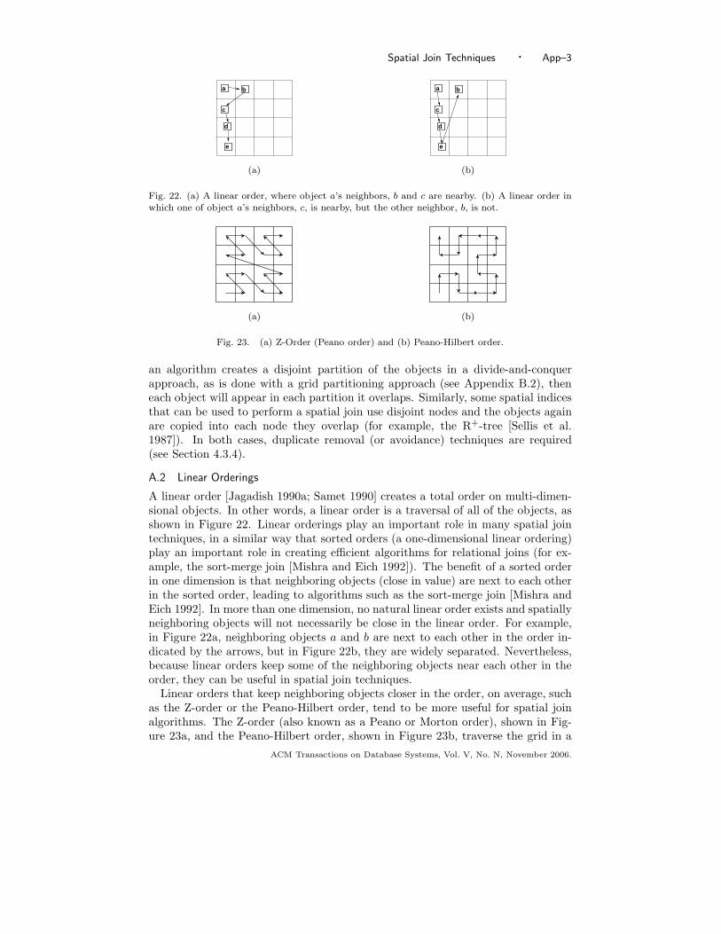
Spatial Join Techniques · App–3
a
c
d
e
b a
c
d
e
b
(a) (b)
Fig. 22. (a) A linear order, where object a’s neighbors, b and c are nearby. (b) A linear order inwhich one of object a’s neighbors, c, is nearby, but the other neighbor, b, is not.
(a) (b)
Fig. 23. (a) Z-Order (Peano order) and (b) Peano-Hilbert order.
an algorithm creates a disjoint partition of the objects in a divide-and-conquerapproach, as is done with a grid partitioning approach (see Appendix B.2), theneach object will appear in each partition it overlaps. Similarly, some spatial indicesthat can be used to perform a spatial join use disjoint nodes and the objects againare copied into each node they overlap (for example, the R+-tree [Sellis et al.1987]). In both cases, duplicate removal (or avoidance) techniques are required(see Section 4.3.4).
A.2 Linear Orderings
A linear order [Jagadish 1990a; Samet 1990] creates a total order on multi-dimen-sional objects. In other words, a linear order is a traversal of all of the objects, asshown in Figure 22. Linear orderings play an important role in many spatial jointechniques, in a similar way that sorted orders (a one-dimensional linear ordering)play an important role in creating efficient algorithms for relational joins (for ex-ample, the sort-merge join [Mishra and Eich 1992]). The benefit of a sorted orderin one dimension is that neighboring objects (close in value) are next to each otherin the sorted order, leading to algorithms such as the sort-merge join [Mishra andEich 1992]. In more than one dimension, no natural linear order exists and spatiallyneighboring objects will not necessarily be close in the linear order. For example,in Figure 22a, neighboring objects a and b are next to each other in the order in-dicated by the arrows, but in Figure 22b, they are widely separated. Nevertheless,because linear orders keep some of the neighboring objects near each other in theorder, they can be useful in spatial join techniques.
Linear orders that keep neighboring objects closer in the order, on average, suchas the Z-order or the Peano-Hilbert order, tend to be more useful for spatial joinalgorithms. The Z-order (also known as a Peano or Morton order), shown in Fig-ure 23a, and the Peano-Hilbert order, shown in Figure 23b, traverse the grid in a
ACM Transactions on Database Systems, Vol. V, No. N, November 2006.

App–4 · E.H. JACOX and H. SAMET
A B
C D
A B
C D
A
B
C D
Entire Space
1 2
3 4
5 6
7 8
9 10
11 12
13 14
15 16
(a) (b) (c)
A
Entire Space
1 2 3 4
B
5 6 7 8
C
9 10 11 12
D
13 14 15 16
(d)
Fig. 24. (a) A four cell grid traversed in a Z-order. (b) A sixteen cell grid traversed in a Z-order.(c) A sixteen cell grid traversal that includes enclosing blocks (lettered blocks). (d) A sixteen cellgrid traversal as a tree traversal.
pattern that helps to preserve locality. They are also known as space-filling curves(see [Samet 2006] for other such curves). Both of these linear orders first orderobjects in a block before moving to the next block. For example, the Z-order is atraversal through a regular grid using a ‘Z’ pattern, as shown in Figure 24a. If thereare more than four cells in the grid, then each top-level block is fully traversed be-fore moving to the next block. In Figure 24b, block A from Figure 24a is traversedin a ‘Z’ pattern before moving to block B. This pattern is repeated at finer levels,where a block at any level is fully traversed before moving to the next block. Inthis way, a linear order is imposed on the cells. The Peano-Hilbert order is similar,as shown in Figure 23b, though each block is traversed in a rotation that might beclockwise or counter-clockwise, avoiding the large jumps between the constituentgrid cells of a Z-order.
Additionally, an order might visit both the grid cells and the enclosing blocks,for instance, ordering both the blocks in Figure 24a and the constituent grid cellsin Figure 24b. To accomplish this order, one convention is to visit enclosing regions(the blocks in Figure 24a) before visiting smaller regions (the cells in Figure 24b),as shown in Figure 24c, which also includes the top level cell (the enclosing space)in the ordering. In essence, this a hierarchical traversal of the nodes, as shown inFigure 24d, which is a preorder tree traversal.
To traverse points in a linear order, the grid cells can be made small enoughsuch that each point is in its own grid cell. To traverse objects in a linear order,either a point in the objects, such as the centroid, is used to represent each objector the objects are assigned to the smallest enclosing block or grid cell, which issimilar to creating an MBR for the object, but with more dead space, as shown inFigure 25a. Note that an object, no matter how small, that intersects the centerpoint will always be in the top level cell (root space), as shown in Figure 25b. Somealgorithms can take advantage of the regular structure of the enclosing cells, but
ACM Transactions on Database Systems, Vol. V, No. N, November 2006.

Spatial Join Techniques · App–5
A
C
B
D
1 2 5 6
3 4 7 8
9 10 13 14
11 12 15 16
r
s
t
(a) (b)
Fig. 25. (a) In a linear ordering, objects can be assigned to the smallest enclosing block or gridcell. Object r is assigned to the root space since it is not within any block. Object s is assigned tothe lower right block, B, and object t is assigned to cell 14. (b) An object overlapping the centerpoint, no matter how small, will be assigned to the top level, which is the entire space.
1 procedure NESTED LOOP JOIN(setA, setB, joinCondition)
2 begin
3 foreach a ∈ setA do
4 foreach b ∈ SetB do
5 if SATISFIED(a, b, joinCondition) then
6 REPORT(a, b);
7 endif;
8 enddo;
9 enddo;
10 end;
Fig. 26. The basic nested loop join with running time O(na · nb), for datasets of size na and nb,using an arbitrary join condition (joinCondition).
1 procedure INDEX NESTED LOOP JOIN(setA, setB)
2 begin
3 spatialIndex←CREATE SPATIAL INDEX(setA);
4 foreach a ∈ setA do
5 spatialIndex.INSERT(a)
6 enddo;
7 foreach b ∈ setB do
8 searchResults←spatialIndex.SEARCH(b)
9 REPORT(searchResults)
10 enddo;
11 end;
Fig. 27. An index nested-loop join improves the performance of the spatial join to O((na + nb) ·log(na) + f), assuming search times of the index are O(log(na) + f), where f is the number ofresults found, na is the size of the indexed dataset, and nb is the size of the unindexed dataset.
at the price of more false hits due to the increased dead space (see Section 3.2 andAppendix B.4).
A.3 Nested Loop Joins
The most basic spatial join method is the nested-loop join, which compares everyobject in one dataset to every object in the other dataset [Mishra and Eich 1992].The algorithm, shown in Figure 26, takes every possible pair of objects and passes itto the SATISFY function to check if the pair of objects meets the given join condition,
ACM Transactions on Database Systems, Vol. V, No. N, November 2006.

App–6 · E.H. JACOX and H. SAMET
termed joinCondition in the algorithm. If a pair satisfies the join condition, thenit is reported using the REPORT function. Given two datasets, A and B, with na andnb objects in each, respectively, the nested-loop join takes O(na ·nb) time. Despitethis larger cost, the nested-loop join can be useful when there are too few objectsto justify the overhead of more complex methods. Note that this algorithm workswith any object type and with any arbitrary join condition.
A variant of the nested-loop join algorithm, called the index nested-loop join [El-masri and Navathe 2000], improves performance for larger datasets by first creatinga spatial index on one dataset, say A. In this algorithm, given in Figure 27, thespatial index is first created and every element of dataset A is inserted into theindex using the INSERT function. Next, the other dataset, say B, is scanned, andeach element is used to search the index on dataset A for intersections. The in-dex is searched using the SEARCH function, which in this context becomes a window
query [Gaede and Gunther 1998] on the index, where the window is the object fromdataset B. Generally, the search window is a rectangle, which limits the types ofjoin conditions to intersection tests or related relations that can be solved with awindow query, such as proximity. Typically, for each object in dataset B, the timeto search the index is, on average, O(log(na) + f), where na is the size of datasetA and f is the number of intersections found. For example, the search and inserttime, on average, for an R-tree [Guttman 1984] is O(log(na) + f). In theory, anobject could intersect every object in the index, creating an O(n) search time. Inpractice though, the number of intersections is small and the running time of theentire algorithm is O((na + nb) · log(na) + f), which includes the time to constructthe index, which is typically O(na · log(na)). Since all of dataset A is inserted first,more efficient static indices and bulk-loading techniques [Arge et al. 1999; Hjaltasonand Samet 1999; Kamel and Faloutsos 1993; van den Bercken et al. 1997] can beused to improve the construction time and the performance of the index.
The index nested-loop algorithm can be executed entirely in memory, using inmemory indices, and is useful as a component in other spatial join algorithms (seeSection 4). The algorithm can also be used as a stand alone external memory spatialjoin algorithm by using external memory indices, which allows the algorithm toprocess larger datasets. For instance, Becker et al. [1993] used grid files [Nievergeltet al. 1984] as the index and Henrich and Moller [1995] used an LSD tree [Henrichet al. 1989] as the index. However, more sophisticated methods exist for using anexternal spatial index to perform a spatial join (see Section 4).
B. NEITHER DATASET INDEXED TECHNIQUES
This Appendix provides more details of specific methods for performing a spatialjoin on unindexed data that were mentioned in Section 4.3. Appendix B.1 discussesan extension to the plane-sweep algorithm (Section 3.1) that can process datasets ofany size by using external memory. Next more sophisticated partitioning algorithmsfrom the literature are described, grouped by how they partition the data: usinggrids in Appendix B.2, using strips in Appendix B.3, by size in Appendix B.4, andclustering in Appendix B.5.
ACM Transactions on Database Systems, Vol. V, No. N, November 2006.

Spatial Join Techniques · App–7
1 procedure EXTERNAL PLANE SWEEP(setA, setB)
2 begin
3 mergedSet←SET MERGE(setA, setB);
4 sortedSet←SORT BY LEFT SIDE(mergedSet);
5 insertList←sortedSet;
6 sweepStructureA←CREATE SWEEP STRUCTURE();
7 sweepStructureB←CREATE SWEEP STRUCTURE();
8 while insertList 6= ∅ do
9 sweepStructureA.INITIALIZE();
10 sweepStructureB.INITIALIZE();
11 doOverFile←new File();
12 foreach r in sortedSet do
13 if r ∈ setA then
14 sweepStructureB.REMOVE INACTIVE(r);
15 sweepStructureB.SEARCH(r);
16 if r = insertList.FIRST() then
17 insertList.POP();
18 errorStatus←sweepStructureA.INSERT(r);
19 if errorStatus = InsufficientMemoryError then
20 doOverFile.WRITE(r);
21 endif;
22 endif;
23 else
24 sweepStructureA.REMOVE INACTIVE(r);
25 sweepStructureA.SEARCH(r);
26 if r = insertList.FIRST() then
27 insertList.POP();
28 errorStatus←sweepStructureB.INSERT(r);
29 if errorStatus = InsufficientMemoryError then
30 doOverFile.WRITE(r);
31 endif;
32 endif;
33 endif;
34 enddo;
35 insertList←doOverFile.READ ENTIRE FILE();
36 enddo;
37 end;
Fig. 28. An external memory version of the plane-sweep algorithm with the ability to processdatasets of any size.
B.1 External Plane Sweep
Jacox and Samet [2003] extended the modified plane-sweep algorithm of Arge etal. [1998] (see Section 3.1) to process datasets of any size by using external memory.The algorithm, shown in Figure 28, adds an outer loop to the plane-sweep algorithmthat keeps track of which objects have been inserted into the sweep structure.Initially, all objects are included in the list of objects to insert, which are stored inthe insertList variable. In the first pass of the outer loop, the plane-sweep runsnormally. If there is sufficient internal memory, the external plane-sweep performsexactly as the internal version (see Figure 2), and the outer loop does not need tobe run again. However, if internal memory is full, then the current object is notinserted into the sweep structure, but marked as not having been added to the sweepstructure. In this case, a reference to the object is saved to a file (or some other
ACM Transactions on Database Systems, Vol. V, No. N, November 2006.

App–8 · E.H. JACOX and H. SAMET
Partition 1
Partition 2
Partition 3
2,3
1, 2, 3
3
1
1
2
1,3
1,2
(a) (b)
Fig. 29. (a) Noncontiguous grid cells are grouped to form three partitions. (b) Forming partitionsfrom noncontiguous grid cells helps to prevent data skew problems by creating partitions of equalsize. Even though the data is clustered in the lower left corner, the partitioning scheme results ineach partition containing either four or five objects. Each object is labeled with the partitions inwhich it will be placed.
external memory storage), called doOverFile. When a pass of the plane-sweepfinishes, this list of objects in doOverFile serves as the list of objects to insert intothe sweep structure in the next pass of the outer loop, which just performs thesame plane-sweep again, but doesn’t insert the objects that were inserted on thefirst pass. The plane-sweep algorithm is run repeatedly until all objects have beeninserted into the sweep structure. Note that on every pass, every object is used tosearch the sweep structure, thereby not missing any intersecting pairs. Also notethat the algorithm merges the two datasets into one dataset at the beginning of thealgorithm with the SET MERGE function so that the algorithm only needs to manageone doOverFile instead of two.
B.2 Partitioning Using Grids
No technique uses a simple grid as did the generic algorithm in Figure 13, sinceit is only useful for uniform distributions. However, Patel and Dewitt [1996] usea uniform grid as a starting point. First, the data space is divided into a uniformgrid, where the number of grid cells, which they call tiles, is greater (typically muchgreater) than the number of desired partitions. The grid cells are then grouped intopartitions using a mapping function in such a way as to minimize skew by, hopefully,creating partitions that contain a similar numbers of objects. For example, inFigure 29a, the grid cells are grouped to form three partitions. Even if the data isskewed, each partition will cover part of the dataset, as shown in Figure 29d. Notethat the data is not physically partitioned into the grid cells, but only into the finalpartitions. In other words, grid cells are assigned to partitions first, and then thedata is partitioned.
Patel and Dewitt [1996] do not proscribe a particular mapping, but only suggestusing some form of a hashing function to assign the cells to partitions. The hashfunction should be chosen to distribute the data evenly amongst the partitionsand is dependent on the dataset. As an example, Patel and Dewitt use a round-robin order, that scans the grid in row-major order and alternates assigning the cellsamong the partitions, as is shown in Figure 29a. In the figure, because the grid cellsare not contiguous, the partitions have a larger total perimeter, leading to increaseddata replication since a larger perimeter provides more opportunities for an object
ACM Transactions on Database Systems, Vol. V, No. N, November 2006.

Spatial Join Techniques · App–9
Sweep Line
Sort/Sweep Direction
Strip 1
Strip 2
Strip 3
Strip 4
Fig. 30. In strip partitioning, the data is partitioned into strips and sorted parallel to the stripto take advantage of the plane-sweep modification described in Section 3.1. In this example, thesweep is repeated four times, once for each strip. The actual height of the sweep line is the heightof the strip.
to intersect the perimeter. Using more initial grid cells increases the uniformityof the distribution because areas of skewed, dense data are distributed amongstseveral partitions, but using more grid cells also increases the replication of objectsacross partitions. Experiments [Patel and DeWitt 1996] showed that increasing thenumber of grid cells can create near uniform distributions from skewed datasets, butthe replication rate can also increase rapidly. In their experiments, Patel and Dewitt[1996] found that Tiger data [U.S. Bureau of the Census 1992] had a replicationrate of about 2.5% with 100 grid cells per partition while Sequoia data [Stonebrakeret al. 1993] had a replication rate of 10%.
Zhou et al. [1997] use a variation of this technique in which the data is physicallypartitioned into the grid cells, first. Since the grid cell sizes are known, the parti-tions can be formed by grouping contiguous cells until a desired partition size, asdetermined using methods from Section 4.3.2, is reached. This approach reducesthe amount of replication because the partition boundary is smaller. The cells canbe grouped using any linear order, such as a Z-order (Appendix A.2). If any gridcells remain after the maximum number of partitions have been formed, then theycan be assigned to the partitions with the least objects.
B.3 Partitioning With Strips
Arge et al. [1998] partition the data into strips so that they can take advantage oftheir modification to the plane-sweep algorithm (Section 3.1). They show a lowerbound for their method of O(n logm(n)+t) I/O transfers, which is optimal, where nis the number of objects in both sets divided by the block size, B (that is, n = N/B,where N is the total number of objects in the datasets), m is the amount of internalmemory divided by block size, and t is the number of result pairs divided by blocksize. For the plane-sweep method, after the data is sorted, it is partitioned intostrips that are parallel to the sort direction, as shown in Figure 30 17. With themodified plane-sweep method, the amount of data that can be processed with agiven amount of internal memory is limited by the maximum size of the active set.When the data is partitioned into strips, the maximum size of the active set is themaximum number of objects that intersect the sweep line, which is a function of
17Guting and Schilling [1987] also used a form of strip partitioning to solve the rectangle inter-section problem using external memory.
ACM Transactions on Database Systems, Vol. V, No. N, November 2006.
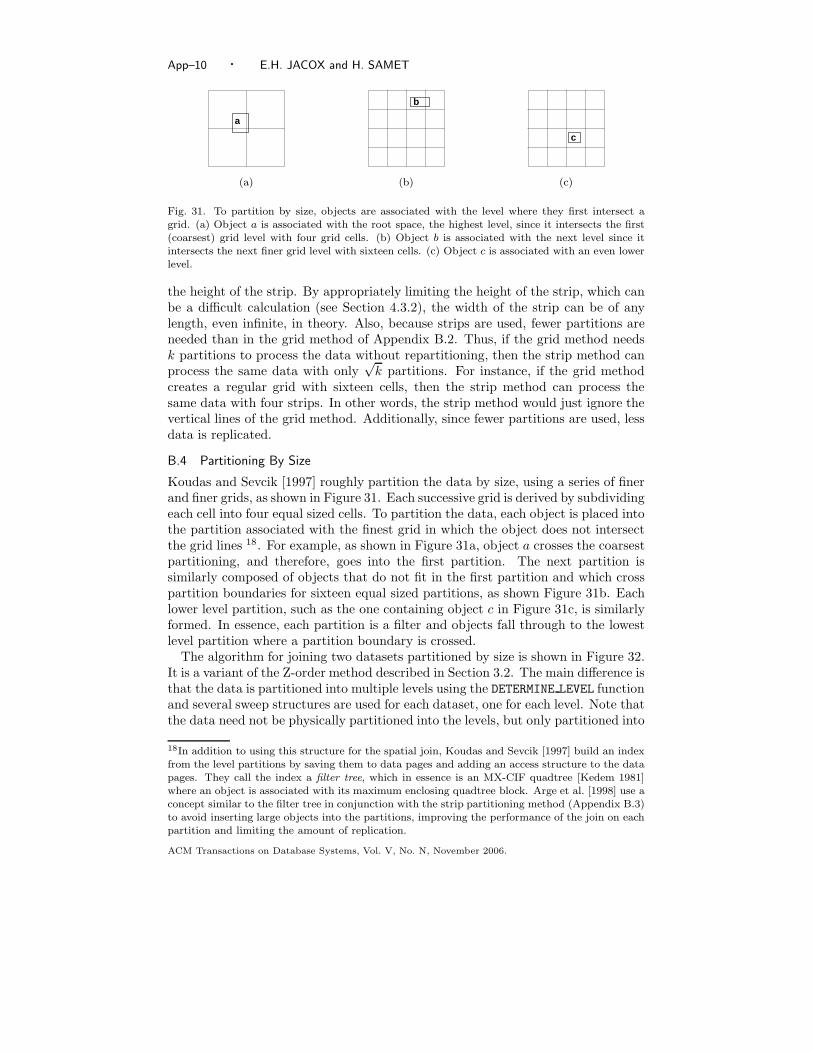
App–10 · E.H. JACOX and H. SAMET
a
b
c
(a) (b) (c)
Fig. 31. To partition by size, objects are associated with the level where they first intersect agrid. (a) Object a is associated with the root space, the highest level, since it intersects the first(coarsest) grid level with four grid cells. (b) Object b is associated with the next level since itintersects the next finer grid level with sixteen cells. (c) Object c is associated with an even lowerlevel.
the height of the strip. By appropriately limiting the height of the strip, which canbe a difficult calculation (see Section 4.3.2), the width of the strip can be of anylength, even infinite, in theory. Also, because strips are used, fewer partitions areneeded than in the grid method of Appendix B.2. Thus, if the grid method needsk partitions to process the data without repartitioning, then the strip method canprocess the same data with only
√k partitions. For instance, if the grid method
creates a regular grid with sixteen cells, then the strip method can process thesame data with four strips. In other words, the strip method would just ignore thevertical lines of the grid method. Additionally, since fewer partitions are used, lessdata is replicated.
B.4 Partitioning By Size
Koudas and Sevcik [1997] roughly partition the data by size, using a series of finerand finer grids, as shown in Figure 31. Each successive grid is derived by subdividingeach cell into four equal sized cells. To partition the data, each object is placed intothe partition associated with the finest grid in which the object does not intersectthe grid lines 18. For example, as shown in Figure 31a, object a crosses the coarsestpartitioning, and therefore, goes into the first partition. The next partition issimilarly composed of objects that do not fit in the first partition and which crosspartition boundaries for sixteen equal sized partitions, as shown Figure 31b. Eachlower level partition, such as the one containing object c in Figure 31c, is similarlyformed. In essence, each partition is a filter and objects fall through to the lowestlevel partition where a partition boundary is crossed.
The algorithm for joining two datasets partitioned by size is shown in Figure 32.It is a variant of the Z-order method described in Section 3.2. The main difference isthat the data is partitioned into multiple levels using the DETERMINE LEVEL functionand several sweep structures are used for each dataset, one for each level. Note thatthe data need not be physically partitioned into the levels, but only partitioned into
18In addition to using this structure for the spatial join, Koudas and Sevcik [1997] build an indexfrom the level partitions by saving them to data pages and adding an access structure to the datapages. They call the index a filter tree, which in essence is an MX-CIF quadtree [Kedem 1981]where an object is associated with its maximum enclosing quadtree block. Arge et al. [1998] use aconcept similar to the filter tree in conjunction with the strip partitioning method (Appendix B.3)to avoid inserting large objects into the partitions, improving the performance of the join on eachpartition and limiting the amount of replication.
ACM Transactions on Database Systems, Vol. V, No. N, November 2006.

Spatial Join Techniques · App–11
1 procedure PARTITION BY SIZE(setA, setB)
2 begin
3 /* determine number of levels */
4 minSize←FIND SMALLEST OBJECT(setA, setB);
5 levels←CEILING(log4(TotalArea/minSize));
6 listA←SORT IN Z-ORDER(setA);
7 listB←SORT IN Z-ORDER(setB);
8 sweepStructuresA[]←CREATE SWEEP STRUCTURES(levels);
9 sweepStructuresB[]←CREATE SWEEP STRUCTURES(levels);
10 while NOT listA.END() OR NOT listB.END() do
11 /* get next rectangle from the two lists */
12 if listA.FIRST() < listB.FIRST() then
13 object←listA.POP();
14 level←DETERMINE LEVEL(object)
15 sweepStructuresA[level].INSERT(object);
16 for( i=level; i<=0; i-- ) do
17 sweepStructuresB[i].REMOVE INACTIVE(object);
18 sweepStructuresB[i].SEARCH(object);
19 enddo;
20 listA.NEXT();
21 else
22 object←listB.POP()
23 level←DETERMINE LEVEL(object)
24 sweepStructuresB[level].INSERT(object);
25 for( i=level; i<=0; i-- ) do
26 sweepStructuresA[i].REMOVE INACTIVE(object);
27 sweepStructuresA[i].SEARCH(object);
28 enddo;
29 listB.NEXT();
30 endif;
31 enddo;
32 end;
Fig. 32. A modified Z-order algorithm that partitions the data by size.
distinct sweep structures, which is a modification suggested by Dittrich and Seeger[2000]. The first step in the algorithm is to determine how many levels are needed,which is done with a simple calculation. The smallest grid cells should be about thesame size as the smallest object, which is found using the FIND SMALLEST OBJECT
function. The number of levels then is roughly the base four logarithm of the totalnumber of grid cells at the finest level, which is estimated as the enclosing area ofthe data space, TotalArea, divided by the size of the smallest object, minSize. Thealgorithm then proceeds nearly identically to the Z-order method from Section 3.2,accounting for multiple sweep structures. Each object is read (in Z-order) andinserted into its dataset’s sweep structure for its level using the INSERT function.Next, after the inactive objects are removed using the REMOVE INACTIVE function,the sweep structures for the other dataset are searched for intersections using theSEARCH function. Only sweep structures at the same level or shallower (coarser)need to be searched since the Z-order can ensure that larger objects will be seenfirst. For instance, the two root space sweep structures will be searched after everyinsertion of the opposing data set.
The finest level partition needed depends on the size of the smallest objects.
ACM Transactions on Database Systems, Vol. V, No. N, November 2006.

App–12 · E.H. JACOX and H. SAMET
The algorithm in Figure 32 assumes that all of the coarser levels contain objects,but this might not be the case. The algorithm can be modified to ignore emptylevels. Note that because the objects are partitioned by size, they are not replicatedbetween partitions. Also, there is no way to repartition the data. Since the sizesof partitions are determined by grid divisions and not by the number of objectsin each partition, there could be too many objects in a particular partition andthe sweep structures could overflow the available internal memory. However, intheir experiments, Koudas and Sevcik [1997] found that sweep structures, whichthey implemented as stacks, tend to contain few objects, and internal memory isunlikely to overflow.
Small objects might be in level partitions meant for larger objects if they crosspartition boundaries for that level, as was shown in Figure 25b in Appendix A.2.This hinders performance. Dittrich and Seeger [2000] suggest replicating smallobjects to allow them to be placed into more appropriate partitions. If an objectis smaller than the grid cells of the boundary that it overlaps, then the object isdivided using the boundary. Each divided piece is then used to find a finer levelpartition in which to insert the full object. For example, the object in Figure 25bwould be divided into four pieces and inserted into the four middle partitions.Duplicate removal methods will then be needed (see Section 4.3.4).
B.5 Data-Centric Partitioning
Lo and Ravishankar [1995; 1996] cluster the data into partitions. One of thedatasets, say dataset A, is first sampled and a nearest-center heuristic is used toidentify clusters of the sampled objects. The centroids of the clusters form the basisof the partitions. Initially, each partition is just the identified point, with no area.As objects from dataset A are inserted into the partitions, the partition boundariesare expanded to enclose the inserted objects. Thus, a partition boundary is theenclosing MBR of the objects in the partition. Data is inserted into the partitionsusing a choice of heuristics, such as inserting into the partition whose size grows theleast by area or into the partition whose centroid is closest. Note that this processresults in non-disjoint partitions. Once dataset A is inserted into the partition,the resulting partition boundaries are used to partition the second dataset, say B.Objects from dataset B are inserted into each partition that they overlap. Eachpartition for dataset A then needs to be joined with only one partition from datasetB using any appropriate internal memory method (Section 3). Duplicate resultsdo not occur since each object from dataset A is only in one partition. One benefitof building non-disjoint partitions is that the partitions might not cover the entiredata space. If this is the case with dataset A, then objects from dataset B that donot overlap any partition can be discarded since they could not be joined with anyobject in dataset A.
C. FILTERING EXTENSIONS
This section discusses approximations other than MBRs that can be used for fil-tering, and a method for making the filtering phase non-blocking. Appendix C.1surveys techniques for producing better candidate sets with fewer false hits by usingbetter approximations. Appendix C.2 discusses tests and approximations that canbe used to identify true hits, that is, pairs of objects that definitely intersect. These
ACM Transactions on Database Systems, Vol. V, No. N, November 2006.

Spatial Join Techniques · App–13
(a) (b) (c)
(d) (e)
Fig. 33. Alternate approximations to MBRs include: (a) the rotated minimum bounding rectangle,(b) the minimum bounding circle, (c) the minimum bounding ellipse, (d) the convex hull, and (e)the minimum bounding n-corner polygon (for example, 5-corner).
pairs can be immediately reported and then removed from the candidate set, mean-ing that they are not passed to the more expensive refinement stage. Appendix C.3describes a technique for making the filtering phase non-blocking.
C.1 False Hit Filtering
The MBR is not the only approximation that can be used during the filteringstage. Other approximations can be used if the filtering method is adapted touse the alternate approximation. Additionally, other approximations can be usedas a secondary filter after the initial filtering stage to prune some false hits fromthe candidate set. To do this, the candidate set is scanned and an intersectiontest is performed on each pair of objects using a different approximation than wasused to do the initial filtering. This second approximation should be stored sincecalculating the approximation on the fly requires the full object to be read intomemory.
Brinkhoff et al. [1993] investigated false hit filtering methods that use approxi-mations other than the MBR, which are shown in Figure 33. The approximationsare:
(1) The rotated minimum bounding rectangle.
(2) The minimum bounding circle.
(3) The minimum bounding ellipse.
(4) The convex hull.
(5) The minimum bounding n-corner polygon (for example, 5-corner).
They found that using a better approximation generally reduces the number offalse hits. The convex hull and 5-corner approximation performed especially well.However, the higher storage costs, the increased complexity of calculating the ap-proximation, and the increased complexity of the intersection test can mitigate the
ACM Transactions on Database Systems, Vol. V, No. N, November 2006.

App–14 · E.H. JACOX and H. SAMET
(a)
Covered
Mostly Covered
Partially Covered
Not Covered
(b)
Fig. 34. An object (a) is approximated using a four color scheme (b) by imposing a grid over theobject and coloring the cells depending on whether they are covered, mostly covered, partiallycovered, or not covered.
Fig. 35. An MBR approximation can be improved by adding two more sides, parallel to eachother.
benefit. Even so, Brinkhoff and Kriegel [1994a] found that additional filtering withthese approximations can improve total performance significantly.
Zimbrao and de Souza [1998] propose using a 4-color raster approximation forsecondary filtering. As shown in Figure 34, a grid is imposed over each objectand grid cells are colored depending on whether they are covered, mostly covered,partially covered, or not covered. To check for intersections, the two raster ap-proximations of the objects are compared, taking into account the different offsetsand scales of the grids. The number of grid cells can be adjusted to obtain moreaccurate results for filtering, but at the expense of higher storage costs.
Veenhoff et al. [1995] propose an approximation that is constructed by rotatingtwo parallel lines around the object 19. In other words, two more sides, parallel toeach other, are added by chopping two corners of the MBR, as shown in Figure 35,creating a better approximation than the MBR, but still relatively inexpensive tocalculate, (i.e., O(n)). The tighter approximation reduces the number of false hits.
A number of techniques have been proposed in the spatial indexing, robotics, andcomputer graphics literature for improving the quality of the approximation yieldedby the MBR whose sides are parallel to the axes. For example, an index termedan oriented bounding box tree (OBBTree) (for example, [Gottschalk et al. 1996;Reddy and Rubin 1978]) uses a rotated minimum bounding box; a P-tree [Jagadish1990b] uses an n-corner polygon; a k-DOP data structure [Klosowski et al. 1998],where the number k of possible orientations of the approximation is bounded; anda general spatial filtering mechanism [Brodsky et al. 1995], which attempts to findthe optimal orientations, uses a minimum bounding polybox. The most general
19This approximation is also used by Duncan et al. [2001] in the BAR tree index.
ACM Transactions on Database Systems, Vol. V, No. N, November 2006.

Spatial Join Techniques · App–15
(a) (b) (c)
Fig. 36. An object approximated by: (a) a maximum enclosed circle, (b) a maximum enclosedrectangle, and (c) a maximum enclosed axis-aligned rectangle.
solution is the convex hull, which is often approximated by a minimum boundingpolygon of a fixed number of sides having either an arbitrary orientation (for ex-ample, the minimum bounding n-corner [Dori and Ben-Bassat 1983; Schiwietz andKriegel 1993]) or a fixed orientation, usually parallel to the coordinate axes (forexample, [Esperanca and Samet 1997]). The minimum bounding box may also bereplaced by a circle, sphere (for example, the sphere tree [Hubbard 1996; Omo-hundro 1989; van Oosterom and Claassen 1990; White and Jain 1996]), ellipse, orintersection of the minimum bounding box with the minimum bounding sphere (forexample, the SR-tree [Katayama and Satoh 1997]). In more than two-dimensions,Kriegel et al. [2004] present approximations for high-resolution three-dimensionalobjects.
In addition to alternate approximations, Koudas and Sevcik [1997] propose anadditional filtering mechanism that might be useful for sparser datasets. Theypropose building a bitmap for one of the datasets, say A, where each bit representsa cell in a fine grid over the data space. If any object from dataset A intersects agrid cell, then the bit is turned on for that cell. Then, as objects from the seconddata are processed, each object is checked against the bit map. If the object doesnot intersect a cell with the bit turned on, then the object can be discarded.
C.2 True Hit Filtering
The traditional filtering phase identifies a candidate set, which is a super set ofintersecting objects that also includes pairs of objects that do not intersect, butwhose approximations intersect. In true hit filtering, additional approximations areused to find object pairs that definitely intersect, termed true hits, and thus can bereported immediately or later combined with the results of the refinement stage.While reducing the size of the candidate set is beneficial, Brinkhoff and Kriegel[1994a] point out that multiple filters might not combine well, that is, adding morethan one filter might not significantly improve performance.
To identify true hits, Brinkhoff and Kriegel [1994a] propose using what they call aprogressive approximation, where the approximation is entirely enclosed by the fullobject. In contrast to enclosing approximations, such as the MBR, the progressiveapproximation does not include extra dead space, but rather excludes portions ofthe full object. If the progressive approximations of two objects intersect, thenthe full objects must intersect. Brinkhoff and Kriegel [1994a] investigated threedifferent progressive approximations, shown in Figure 36:
ACM Transactions on Database Systems, Vol. V, No. N, November 2006.

App–16 · E.H. JACOX and H. SAMET
Fig. 37. If the MBRs of two objects cross, then the two objects must intersect.
(1) A maximum enclosed circle.
(2) A maximum enclosed rectangle.
(3) A maximum enclosed axis-aligned rectangle.
These approximations were shown to be effective at identifying true hits, but theyare more expensive to calculate than MBRs and require extra storage space.
Brinkhoff and Kriegel [1994a] also describe a cross test that looks for enclosingapproximations, such as MBRs, that cross, as shown in Figure 37 20. For example,assuming the objects are contiguous, if the MBRs of two objects cross, then theobjects must intersect. This is because the objects must also cross at some pointand thereby intersect. This is most clearly seen by trying to imagine a counterexample where the MBRs cross, as in Figure 37, without the objects intersecting.In their experiments, Brinkhoff and Kriegel found that very few intersecting MBRswill cross. However, they argue that since the cross test is so simple, it is worthapplying, even if it identifies only a few true hits.
C.3 Non-Blocking Filtering
During the filtering phase, any algorithm will block while building an index, sortingthe data, or partitioning the data. No output will be produced while this occurs,which delays overall processing in a pipelined system [Graefe 1993]. This sectionfirst describes a variant of the index nested-loop join (Appendix A.3) which is non-blocking and then presents a method to make any filtering technique non-blocking.
The indexed nested-loop join in Appendix A.3 blocks while it is building an index,that is, it doesn’t produce any result pairs, which can slow processing in pipelinedsystems [Graefe 1993]. To overcome this limitation, Luo et al. [2002] use a non-blocking variation of the index nested-loop join so that some results are returnedimmediately. In the algorithm, shown in Figure 38, each dataset is indexed usinga dynamic index, such as an R-tree [Guttman 1984]. A dynamic index must beused, which can be less efficient than static indices, but static indices block whilebeing built. The input to the algorithm is the combined datasets. If the datasetsare separate, as shown in previous algorithms, then either one data element orblocks of elements should be read from each dataset, alternating between the twodatasets. Otherwise, no results will be reported until items from the second datasetare encountered. As each element is encountered, it is inserted into the index
20The cross test is similar to the intersection test of Ballard [1981] and Peucker [1976].
ACM Transactions on Database Systems, Vol. V, No. N, November 2006.

Spatial Join Techniques · App–17
1 procedure NON-BLOCKING NESTED LOOP JOIN(combinedDataSets)
2 begin
3 spatialIndexA←INTIALIZE DYNAMIC SPATIAL INDEX();
4 spatialIndexB←INTIALIZE DYNAMIC SPATIAL INDEX();
5 foreach dataElement ∈ combinedDataSets do
6 if dataElement ∈ setA then
7 spatialIndexA.INSERT(dataElement)
8 intersections←spatialIndexB.SEARCH(dataElement)
9 else
10 spatialIndexB.INSERT(dataElement)
11 intersections←spatialIndexA.SEARCH(dataElement)
12 endif;
13 REPORT(intersections)
14 enddo;
15 end;
Fig. 38. A non-blocking index nested loop join allows results to be reported immediately andcontinuously.
belonging to it’s own dataset and the other index is searched for intersections. Inthis way, results can appear after only a few objects have been seen, though at theexpense of building a second index.
A similar technique can be used to make any filtering technique non-blocking.Luo et al. [2002] propose a simple extension, that is conceptually similar to apipelining hash join [Wilschut and Apers 1991], and is applicable to most filteringmethods. They propose devoting a portion of internal memory to maintaining anin-memory R-tree (or any other spatial index) for each dataset, say datasets A andB, and then using the non-blocking nested loop join as a front-end to the filteringmethod. Only a subset of datasets A and B is inserted into the R-trees, whichis processed like the non-blocking nested loop join shown in Figure 38. Once theR-trees are full, that is, the allotted internal memory is used up, the remaining datais processed using a more efficient external memory method (Section 4). However,the R-trees are still searched using the remaining objects in order to find all ofthe intersections with the objects in the indices. Once all of the data has beenencountered, the objects in the indices can be discarded since all intersections withthem have been reported, thereby freeing more internal memory for use by theexternal memory method used for the remaining objects.
D. THE REFINEMENT STAGE
The filtering stage (Section 4) produces a set of candidate object pairs that aretypically represented as pairs of object ids. The candidate set contains pairs whoseapproximations intersect, but do not necessarily intersect themselves. The refine-ment stage checks the full objects to remove any of these false hits from the can-didate set. Unless all of the full objects in the candidate set can fit into internalmemory, the key to the refinement stage is ordering the reading of the full objectsto minimize I/O. This issue is discussed in Appendix D.1. Since objects are of-ten polygons, Appendix D.2 describes a common algorithm for checking if a pairof polygonal objects intersect. This test can be performed faster if the polygonsare indexed using a spatial access method [Gaede and Gunther 1998; Samet 1990],
ACM Transactions on Database Systems, Vol. V, No. N, November 2006.

App–18 · E.H. JACOX and H. SAMET
which is discussed in Appendix D.3.The candidate set might contain duplicate results, which should be removed first
to avoid any extra intersection tests on the full objects. If online techniques forduplicate removal are used (Section 4.3.4), then the candidate set will not containany duplicate results. However, some methods cannot use the online techniquesand will introduce duplicates into the candidate set. A straight-forward approachto duplicate removal is to sort the id pair list, then scan the list and remove theduplicates. This extra step might not impact performance because it can be com-bined with techniques for efficiently reading the full objects from external memoryin order to do the full object intersection tests, as discussed in Appendix D.1.
D.1 Ordering Pairs
Before performing an intersection test on a pair of objects, each object must be readinto memory. Since the full objects might be large, it is unlikely that every objectin the candidate set will fit into internal memory. In the best case, each objectwill be read once, and in the worst case, both objects will need to be read for eachcandidate pair. The pairs can be processed in the order in which the filtering stageproduces them, which is necessary in a pipelined system [Graefe 1993]. Otherwise, ifthe extra cost of sorting is acceptable, then the candidate pairs can be sorted by idsor by the MBRs using a one-dimensional sort or a linear order (see Appendix A.2).Sorting improves performance and avoids the worst case of reading two objects foreach candidate pair by minimizing the number of repeated reads of an object.
When the candidate pairs are not sorted, Abel et al. [1999] showed that thefiltering method used impacts the performance of the refinement stage. In theirexperiments, they showed that the output of Z-order methods (see, for example,Appendix A.1 and Appendix B.4) were processed faster in the refinement stagethan the output of the hierarchical traversal methods (Section 4.1.1). To explainthis phenomenon, they suggest that the Z-order methods produce candidates thathave more locality, making it more likely that the candidate pairs for an object arenear each other in the output order, and thus, the object is more likely to remainin internal memory until it is needed again.
Alternatively, sorting the candidate pairs can reduce the number of times anobject is read into memory, although the cost of sorting the pairs might offset someof the performance benefit. The pairs can be sorted using objects from only onedataset or a combination of both objects, using, for example, the centroid of the twoobjects or the MBR enclosing the two objects. Also, different amounts of internalmemory can be devoted to each dataset, which is similar to the techniques used toread partitions in a non-hierarchical spatial join (Section 4.1.2). In one approach,the candidate pairs can be sorted for one dataset, say R. The objects in datasetR will be read into memory only once, while the objects from the other dataset,say S, will be read a multiple number of times. The objects from dataset S mightbe read as often as once for each candidate set pair, which is still better than theworst case of reading two objects into memory for each candidate pair. In anotherapproach, Patel and Dewitt [1996] modify this process slightly by reading as muchof the sorted dataset R into memory as possible, leaving room for one object fromthe dataset S. Then, the objects from dataset S are read one at a time, testingfor intersections with each object with which it is paired in the candidate set that
ACM Transactions on Database Systems, Vol. V, No. N, November 2006.

Spatial Join Techniques · App–19
1 function EDGE INTERSECTION TEST(edgesA, edgesB, MBRoverlap): boolean
2 begin
3 allEdges←edgesA ∪ edgesB;
4 allEdgesInRegion←EDGES IN REGION(allEdges, MBRoverlap);
5 allEndPoints←DOUBLE EDGES(allEdgesInRegion);
6 edgeList=SORT BY END POINT(allEndPoints);
7 activeEdges←CREATE SWEEP STRUCTURE();
8 while edgeList 6= ∅ do
9 edge←edgeList.POP();
10 edgeAbove←activeEdges.EDGE ABOVE(edge);
11 edgeBelow←activeEdges.EDGE BELOW(edge);
12 if edge is the beginning of the edge then
13 activeEdges.INSERT(edge);
14 if INTERSECT(edge, edgeAbove) OR INTERSECT(edge, edgeBelow) then
15 return true;
16 endif;
17 else
18 if INTERSECT(edgeAbove, edgeBelow) then
19 return true;
20 endif;
21 activeEdges.REMOVE(edge);
22 endif;
23 enddo;
24 return false; /* No intersection detected. */
25 end;
Fig. 39. A plane-sweep algorithm for detecting the intersection of simple polygons whose MBRsintersect.
is present within the portion of dataset R that is in memory. While objects fromdataset R are still read one at a time, objects from dataset S will likely be read lessoften, since on each read, they can be compared to a multiple number of objectsfrom R.
In a more sophisticated approach for polygonal datasets, Xiao et al. [1998] pro-pose clustering the candidate pairs using matrix calculations. In their approach,they pose the read scheduling as an optimization problem that minimizes the num-ber of fetches, weighted by object size. In the matrix, rows represent one datasetand columns represent the other dataset. The matrix values are the sums of thenumber of vertices in two intersecting polygons or zero for non-candidate pairs. Thisapproach, unlike other methods, takes into account object sizes. Matrix calcula-tions, termed the Bond Energy Algorithm, are used to cluster objects into datasetsthat fit in memory, where an object might be in multiple clusters. This algorithmruns in O(n3) time, where n is the number of objects.
D.2 Polygon Intersection Test
If the objects are polygons, a common approach to test if the objects intersect is aplane-sweep technique [Preparata and Shamos 1985], which is conceptually similarto the plane-sweep technique described in Section 3.1. The algorithm, shown inFigure 39, determines if two polygons have any intersecting edges. As with theplane-sweep technique in Section 3.1, this algorithm works by sweeping an axis-aligned line across the plane. The end points of the edges from both polygons
ACM Transactions on Database Systems, Vol. V, No. N, November 2006.

App–20 · E.H. JACOX and H. SAMET
e
ab
Fig. 40. Only the edges contained within the intersecting region of the MBRs could intersect eachother. Edge e of object a, which is outside of the intersecting region, could not possibly intersectobject b.
are the stopping points of the sweep line and the edges intersecting the sweep lineform the active set. If the polygons do not have intersecting edges, one polygoncould be contained within the other and a separate test for containment needs tobe performed, which is described later.
The typical plane-sweep polygon intersection algorithm has been modified toimprove its performance for the refinement stage using a technique of Brinkhoffet al. [1994]. Since only edges within the intersecting region of the MBRs of thetwo polygons could possibly intersect, only those edges are used in the plane-sweepmethod. Any other edges are removed from consideration using the EDGES IN -
REGION function in the algorithm. For example, in Figure 40, edge e of polygona is not contained in the intersecting region of the MBRs and could not possiblyintersect polygon b.
The algorithm has also been simplified by assuming that the polygons are simple,that is, they do not intersect themselves. In the algorithm, as soon as an intersectingedge is found, the algorithm can report that the polygons intersect without checkingif the intersecting edges belong to the same polygon because the polygons aresimple 21.
The first step of the algorithm in Figure 39 combines the edges from both poly-gons into one dataset and removes any edges that do not overlap the intersectingregion of the MBRs, MBRoverlap, using the EDGES IN REGION function. Next, theDOUBLE EDGES function creates two entries for each edge, one for each end point,which are the stopping points of the sweep line. Then, the end points are sortedin one dimension using the SORT BY END POINT function. As with the plane-sweepalgorithm in Section 3.1, a sweep structure is needed to store the edges that inter-sect the sweep line. In this case, the sweep structure, referred to as activeEdges,must perform two additional operations, EDGE ABOVE and EDGE BELOW, which iden-tify edges that intersect the sweep line just above the given edge or just below,respectively. After initializing the activeEdges structure with the CREATE SWEEP -
STRUCTURE function, the list of edges is scanned. When an edge is first encountered,it is inserted into the activeEdges structure, using the INSERT function. Whenthe end of an edge is encountered, it is removed from the activeEdges structure
21Becker et al. [1999] review and propose algorithms for non-simple polygons and efficient algo-rithms for finding all of the intersecting edges.
ACM Transactions on Database Systems, Vol. V, No. N, November 2006.

Spatial Join Techniques · App–21
Sweep Line Position A
1
2
3
4
Sweep LinePosition B
(a)
Sweep Line
1
2
3
4
Edge Above
Edge Below
Inserted Edge
5
(b)
Sweep Line
6
3
4
Edge Above
Edge Below
Deleted Edge
(c)
Fig. 41. (a) Two intersecting edges will intersect the sweep line at adjacent points as the sweepline approaches their intersect point. (b) When an edge is inserted, it could intersect the edgejust above it or below it. (c) When an edge is deleted, the edges adjacent to it might intersect.
a
b
point p
c
Fig. 42. Object a will be reported as contained within object b since the horizontal line througha point, p, in a intersects object b once to the left of point p. Object a will not be reported ascontained within object c since it intersects the horizontal line twice to the left of point p.
using the REMOVE function.In the algorithm, an edge intersection test is performed when an edge is inserted
or removed from the sweep structure. As the sweep line moves, the relative positionsof the intersection points of the sweep line with the edges change. For example,as shown in Figure 41a, the edges intersect the sweep line at position A, in theorder 3, 1, 2, and 4, from top to bottom. At position B, the sweep line does notintersect edges 1 or 2 and edge 3 has moved down the sweep line while edge 4 hasmoved up. The edges continuously change their intersection point with the sweepline as the sweep progresses, but the relative order of the edges only change whenan edge is inserted or removed (or when two edges intersect). Furthermore, onlythe two edges adjacent to the inserted or removed edge will move in the relativeorder. For instance, when edge 5 is inserted in Figure 41b, only edges 2 and 4 havechanged order and are no longer adjacent. Therefore, when an edge is inserted,an intersection test is performed with it and the edge above and the edge belowusing the EDGE ABOVE and EDGE BELOW functions, respectively, to find the edges tobe tested. Similarly, when an edge is deleted, only the relative order of the edgesabove and below it are effected. For instance, when edge 6 is deleted in Figure 41c,edges 3 and 4 become adjacent. Therefore, when an edge is deleted, an intersectiontest is performed between the edge that was above it and the edge that was belowit, using the EDGE ABOVE and EDGE BELOW functions, respectively.
Because the polygons are assumed to be simple, if any edges intersect, thenthe polygons must intersect and true is returned. Otherwise, the sweep completes
ACM Transactions on Database Systems, Vol. V, No. N, November 2006.

App–22 · E.H. JACOX and H. SAMET
Fig. 43. A polygon can be approximated by trapezoids, which can be used to perform a fasterpolygon intersection test.
without finding any intersections and false is returned 22. Since a polygon couldbe contained within the other, a containment test is necessary if false is returnedto confirm that the polygons do not overlap. A containment test [Preparata andShamos 1985], which typically has an O(n) running time, needs to be run twice toconclude that neither object is contained within the other. One such algorithm,briefly described here, takes a point from one polygon, say a, and the edges fromthe other, say b, and checks if the point is contained within the polygon. If so, thena must be contained within b. Any point on or in polygon a will suffice. Using ahorizontal line through the point from polygon a, the algorithm counts the numberof edges of b that intersect the horizontal line to the left of the given point. Asshown in Figure 42, the point is contained within the polygon only if the horizontalline intersects the edges an odd number of times to the left of the point. Thealgorithm concludes by returning true if an odd number of intersections to the leftof the point were detected and false otherwise. Care must be taken in countingintersections with horizontal edges, which can be counted as either no intersectionor as two intersections. Care must also be taken with intersections involving the endpoints of edges, which can be counted as half of an intersection. For more details onthis issue, see the discussion of the point-in-polygon test in any computer graphicsbook, such as [Foley and van Dam 1982].
D.3 An Alternate Intersection Test
To improve the speed of the polygon intersection test, at the expense of higher stor-age costs, a spatial access method can be used to store each full polygon [Gaede andGunther 1998; Samet 1990]. When the polygons are represented by a containmenthierarchy (for example, an R+-tree [Sellis et al. 1987] or a region quadtree [Klinger1971]), a synchronized traversal similar to that described in Section 4.1.1 can beused to check for intersections between the full polygons. For example, Brinkhoff etal. [1994] propose that each full polygon be decomposed into trapezoids, as shownin Figure 43, and storing the pieces in an R∗-tree like structure called a TR∗-tree.The entire TR∗-tree for each polygon is stored with the polygon. When two poly-gons are checked for intersection, both TR∗-trees are read into memory and then
22In the full polygon intersection test, where all of the intersecting edges need to be found orthe polygons are not simple, intersections with adjacent edges also need to be checked when anintersection point occurs since the two edges switch positions in the list, creating new adjacenciesfor the edges. The algorithm shown in Figure 39 just reports success as soon as any intersectionis found since the polygons are simple and will not self-intersect.
ACM Transactions on Database Systems, Vol. V, No. N, November 2006.

Spatial Join Techniques · App–23
a synchronized traversal is performed to check for intersections. This process canbe further improved by using heuristics that detect intersections between partialpolygons [Badawy and Aref 1999; Huang et al. 1997].
ACM Transactions on Database Systems, Vol. V, No. N, November 2006.