Spatial Database &

Spatial Data Mining

Shashi ShekharDept. of Computer Sc. and Eng.

University of Minnesota

shekhar@cs.umn.edu, www.cs.umn.edu/~shekhar

www.spatial.cs.umn.edu

Spatial Data

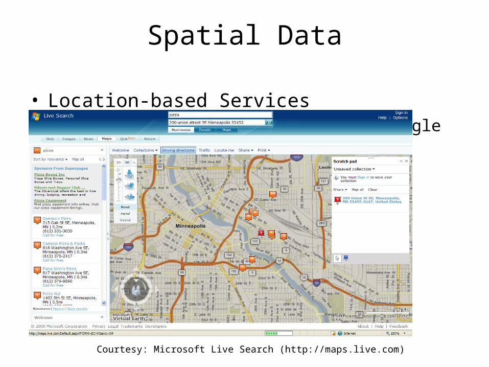
• Location-based Services– E.g.: MapPoint, MapQuest, Yahoo/Google Maps, …

Courtesy: Microsoft Live Search (http://maps.live.com)

Spatial Data

• In-car Navigation Device

Emerson In-Car Navigation System (Courtesy: Amazon.com)

Bookhttp://www.spatial.cs.umn.edu

Outline

• Spatial Databases– Conceptual Modeling

• Pictograms enhanced Entity Relationship Model

– Logical Data Model• Direction predicates and queries

– Physical Data Model• Query Processing – Shortest Paths, Evacuation Routes,

– Correlated time-series

• Storage – Connectivity Clustered Access Method

• Spatial Data Mining– Location Prediction – fast algorithms– Co-location patterns – definition, algorithms– Spatial outliers – algorithms– Hot-spots – new work on “mean streets”

Geo-Spatial Databases: Management and Mining

Nest locations Distance to open water

Vegetation durabilityWater depth

1. Recent book from our group! 3. Shortest Path Queries 4. Storing roadmaps in disk blocks2. Parallelize Range Queries

6. Spatial outlier detect bad sensor (#9) on Highway I-355. Location prediction to characterize nesting grounds.

Spatial Data Mining (SDM)

• The process of discovering– interesting, useful, non-trivial patterns

• patterns: non-specialist• exception to patterns: specialist

– from large spatial datasets

• Spatial pattern families– Spatial outlier, discontinuities– Location prediction models– Spatial clusters– Co-location patterns– …

Spatial Data Mining - Example

Nest locationsDistance to open water

Vegetation durability Water depth

Spatial Autocorrelation (SA)• First Law of Geography

– “All things are related, but nearby things are more related than distant things. [Tobler, 1970]”

• Spatial autocorrelation– Nearby things are more similar than distant things– Traditional i.i.d. assumption is not valid– Measures: K-function, Moran’s I, Variogram, …

Pixel property with independent identical distribution

Vegetation Durability with SA

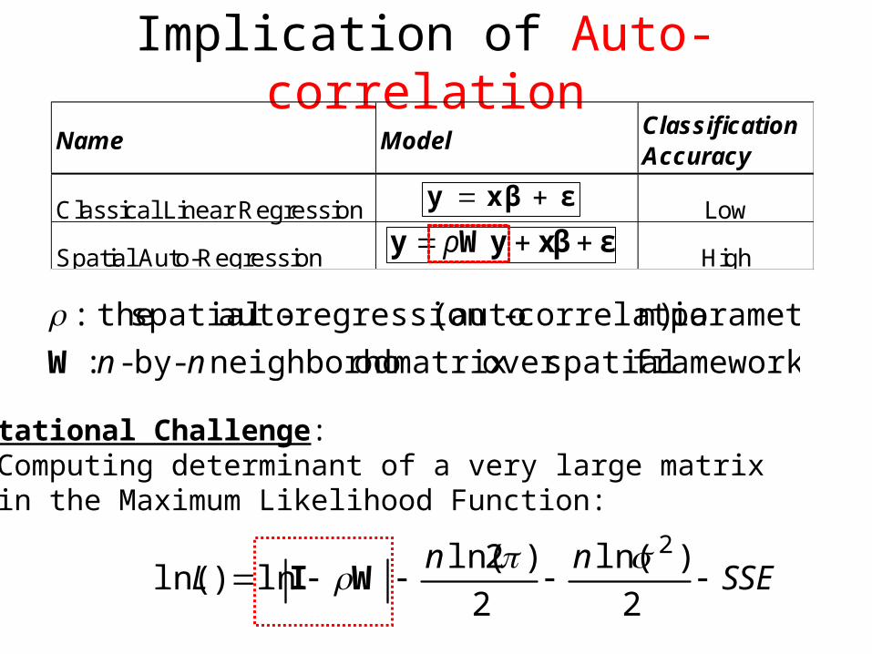
Implication of Auto-correlation

Classical Linear Regression Low

Spatial Auto-Regression High

Name ModelClassification Accuracy

εx βy

εxβWyy ρ

framework spatialover matrix odneighborho -by- :

parameter n)correlatio-(auto regression-auto spatial the:

nnW

SSEnn

L 2

)ln(

2

)2ln(ln)ln(

2WI

Computational Challenge: Computing determinant of a very large matrix in the Maximum Likelihood Function:

Outline

• Spatial Databases– Conceptual Modeling

• Pictograms enhanced Entity Relationship Model

– Logical Data Model• Direction predicates and queries

– Physical Data Model• Query Processing – Shortest Paths, Evacuation Routes,

– Correlated time-series

• Storage – Connectivity Clustered Access Method

• Spatial Data Mining– Location Prediction – fast algorithms– Co-location patterns – definition, algorithms– Spatial outliers – algorithms– Hot-spots – new work on “mean streets”

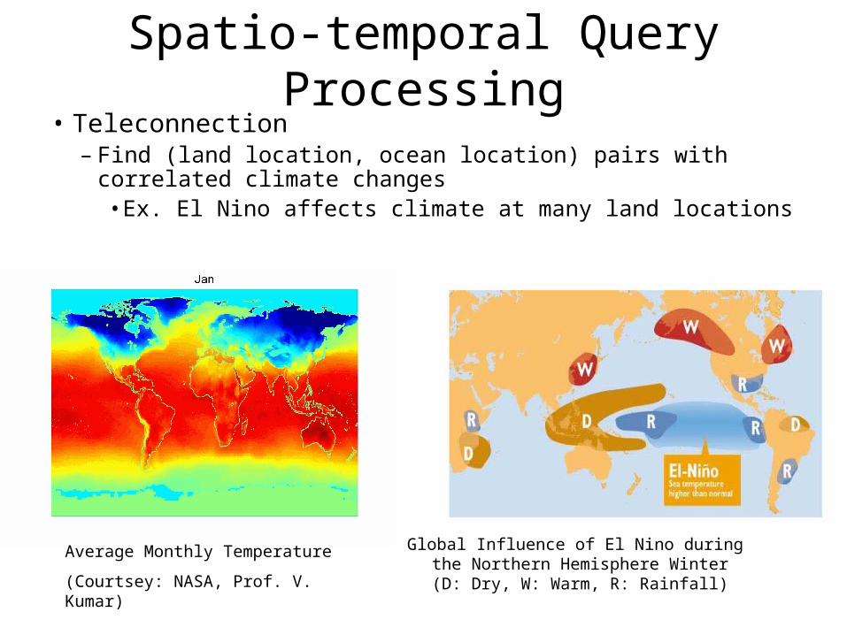
Spatio-temporal Query Processing• Teleconnection

– Find (land location, ocean location) pairs with correlated climate changes• Ex. El Nino affects climate at many land locations

Global Influence of El Nino during the Northern Hemisphere Winter(D: Dry, W: Warm, R: Rainfall)

Average Monthly Temperature

(Courtsey: NASA, Prof. V. Kumar)

Auto-correlation saves computation cost

• Challenge– high dimensional (e.g., 600) feature space– 67k land locations and 100k ocean locations (degree by degree

grid)– 50-year monthly data

• Computational Efficiency– Spatial autocorrelation

• Reduce Computational Complexity

– Spatial indexing to organize locations• Top-down tree traversal is a strong filter

• Spatial join query: filter-and-refine

– save 40% to 98% computational cost at θ = 0.3 to 0.9

Evacuation Route Planning - Motivation

No coordination among local plans means Traffic congestions on all highways e.g. 60 mile congestion in Texas (2005)

Great confusions and chaos

"We packed up Morgan City residents to evacuate in the a.m. on the day that Andrew hit coastal Louisiana, but in early afternoon the majority came back home. The traffic was so bad that they couldn't get through Lafayette." Mayor Tim Mott, Morgan City, Louisiana ( http://i49south.com/hurricane.htm )

Florida, Lousiana (Andrew, 1992)

( www.washingtonpost.com)

( National Weather Services) ( National Weather Services)

( FEMA.gov)

I-45 out of Houston

Houston

(Rita, 2005)

A Real Scenario

Nuclear Power Plants in Minnesota

Twin Cities

Monticello Emergency Planning Zone

Monticello EPZSubarea Population2 4,675 5N 3,9945E 9,6455S 6,7495W 2,23610N 39110E 1,78510SE 1,39010S 4,616 10SW 3,40810W 2,35410NW 707Total 41,950

Estimate EPZ evacuation time: Summer/Winter (good weather):     3 hours, 30 minutesWinter (adverse weather):   5 hours, 40 minutes

Emergency Planning Zone (EPZ) is a 10-mile radius around the plant divided into sub areas.

Data source: Minnesota DPS & DHS Web site: http://www.dps.state.mn.us

http://www.dhs.state.mn.us

A Real World Testcase

Source cities

Destination

Monticello Power Plant

Routes used only by old plan

Routes used only by result plan of capacity constrained routing

Routes used by both plans

Congestion is likely in old plan near evacuation destination due to capacity constraints. Our plan has richer routes near destination to reduce congestion and total evacuation time.

Twin Cities

Experiment Result

Total evacuation time:

- Existing Plan: 268 min.

- New Plan: 162 min.

Outline

• Spatial Databases– Conceptual Modeling

• Pictograms enhanced Entity Relationship Model

– Logical Data Model• Direction predicates and queries

– Physical Data Model• Query Processing – Shortest Paths, Evacuation Routes,

– Correlated time-series

• Storage – Connectivity Clustered Access Method

• Spatial Data Mining– Location Prediction – fast algorithms– Co-location patterns – definition, algorithms– Spatial outliers – algorithms– Hot-spots – new work on “mean streets”

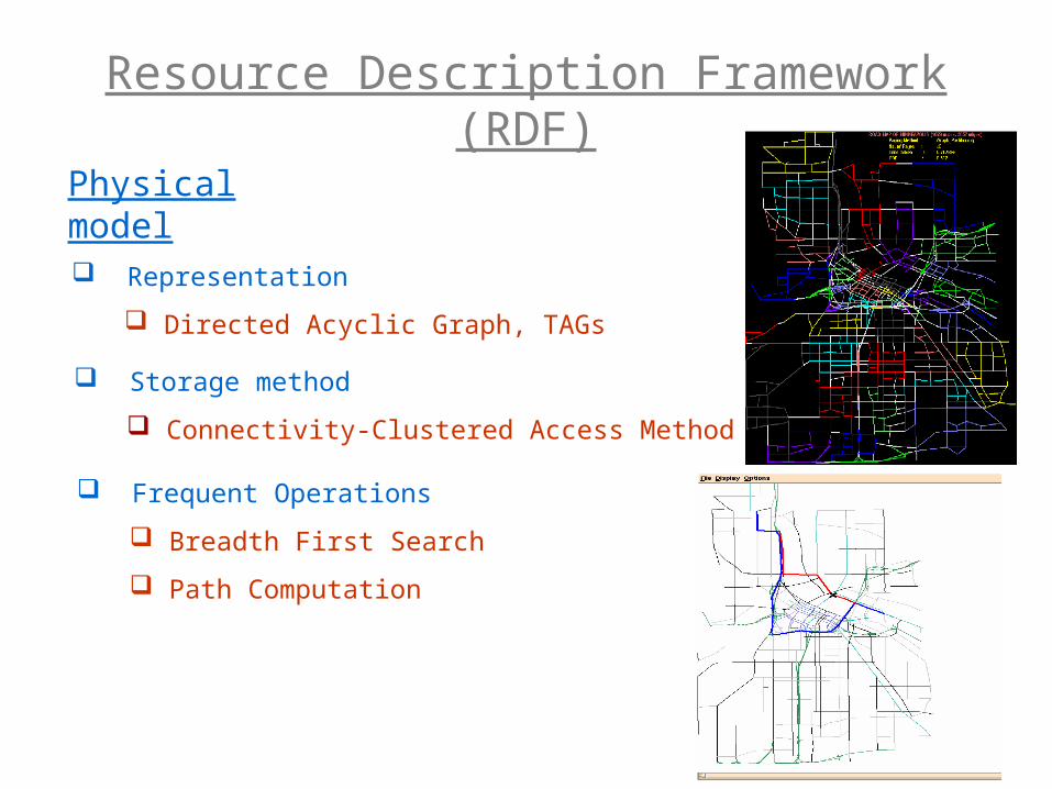
Resource Description Framework (RDF)

Physical model

Representation

Directed Acyclic Graph, TAGs

Storage method

Connectivity-Clustered Access Method (CCAM)

Frequent Operations

Breadth First Search

Path Computation

Semantics in Databases

• Ontology

- Shared Conceptualization of knowledge in a specific domain.

• Resource Description Framework (RDF)

- Representation of resource information in World Wide Web.

• Patterns

Ontology based Semantic Computing

Example Query

SELECT * FROM travelmodeWHERE ONT_RELATED (transport,

‘IS_A’,‘Road’,‘Transport_Ontology’,123) = 1;

Result: All walk and drive modes.

…

Drive Walk

Transport

Road Commuter Rail

Bus

ApplicationsHomeland Security, Life Sciences, Web Services

Resource Description Framework (RDF)Multimodal Transportation System

Commonwealth Ave. and Subway (Green Line), Boston[source: http://maps.google.com/]

Subway Stations

Road Intersections

Transition Edge

N1 N2 N3 N4 N5

R1 R2 R3

Graph Representation

(between BU Central and Blandford St)

Resource Description Framework (RDF)

: Street

: TrafficLight

: RailRoute

: RailRoute

: bus

:busTerminals

: busStops

crosscuts used_by

parallel

has Start/end

halts

Light Rail System

: Rail_line

: Streets

: Streets

start/end

has

serves

crosscuts

parallel

: Terminals

used_by

Road System

: TrafficLight

: Stations

: Trains

Transit Edges(*)

Multimodal Transportation System

: Streets

SELECT S.street, S.busStop, R.Stations, R.RailRoute,R.TerminalFROM TABLE(SDO_RDF_MATCH(

‘(?x : halts ?b)

SDO_RDF_Models(‘rail_line R’,’street S’)),

‘(?rr :serves ? z),

WHERE S.b hasTransitTo R.z and S.Street = ‘Commonwealth’

‘(?rr :start/end ?tr),

Find all routes from the Commonwealth Avenue to the Logan Airport using bus and subway systems.

*Note: A subset of possible transition edges is shown.

and R.terminal = ‘Logan airport’;

Geo-Spatial Databases: Management and Mining

Nest locations Distance to open water

Vegetation durabilityWater depth

1. Recent book from our group! 3. Shortest Path Queries 4. Storing roadmaps in disk blocks2. Parallelize Range Queries

6. Spatial outlier detect bad sensor (#9) on Highway I-355. Location prediction to characterize nesting grounds.