spatial correlations in a transonic jet...spatial correlations in a transonic jet lawrence...
TRANSCRIPT
Spatial Correlations in a Transonic Jet
Lawrence Ukeiley∗
University of Florida, Shalimar, Florida 32579
Charles E. Tinney†
Université de Poitiers, 86034 Poitiers, France
Richa Mann‡
University of Mississippi, University, Mississippi 38677
and
Mark Glauser§
Syracuse University, Syracuse, New York 13244
DOI: 10.2514/1.26071
Particle image velocimetrymeasurements of an unheatedMach 0.85 jet are used to examine its various turbulence
properties. The data are presented from two separate experiments; one with the light sheet orientated in the
streamwise direction (r–x plane) and one with the light sheet perpendicular to the flow direction (r–� plane). The
instrument’s characteristics allow for the calculation and subsequent analysis of the two-point spatial correlations
which are known to be relevant to the source terms in acoustics analogies where sound production is concerned. An
examination of the spatial correlations demonstrates the averaged spatial evolution of the jet’s large-scale turbulent
structures throughout the noise producing region. In particular, the (r–x) spatial dependence of the axial and
azimuthal normal stresses manifest a oblique structure in the mixing layer regions of the flow, whereas the radial
normal stresses evolvemore uniformly toward the end of the potential core. Quadrupole source terms relevant to the
sound productionmechanisms are also calculated fromwhich their spatial distributions are analyzed with zero time
delay. The analysis of these source terms at x=D� 4 showhow the peak energy for the shear-noise component resides
on the high-speed side of the shear layer around r=D� 0:33, whereas the self-noise terms peak along the lip-line at
r=D� 0:5, and aremost energetic for the streamwise and azimuthal components of the velocity. To fully evaluate the
quadrupole sources of noise, the space-time correlations of the full three-dimensional turbulent flowfield are
required which are currently not available from experiments.
I. Introduction
T HE noise generated by the turbulent fluctuations of high-speed,transonic jet plumes represents an important source of sound for
many civilian and military aircraft personnel, especially those whoreside and work in close proximity to active aviation operations.Fundamental studies of these sources have been ongoing essentiallysince the advent of jet aircraft and have concentrated on both theturbulent flow and the acoustic pressure fluctuations that it radiates.Although several decades of research have produced numerousvolumes of literature pertaining to the subject of aerodynamicallygenerated noise, many scientific gaps still reside in identifying theexact nature by which turbulent flows generate sound. Particularlychallenging is the limited information identifying the differencesbetween the turbulent statistics of the “quiet” and “noisy” structuresof a flow [1,2], and under what circumstances do some of thedynamic characteristics (of theflow) play amore significant role thanothers. In hindsight, the recent advancements with computational
capabilities, including the introduction of planar optical techniques,have provided the necessary tools by which identifying (andcontrolling) the sources of sound from high-speed jet flows may beaddressed.
Lighthill [3,4] has been attributed with developing the first theoryby which the turbulent properties of a flow could generate and emitsound. Since this work, there has been a wealth of studies usingnumerical, analytical, and experimental techniques, most of whichhave improved the capabilities of existing tools for capturing andunderstanding the so-called sources of noise. Many reviews ofLighthill’s original work have been performed, including those ofCrighton [5], Ffowcs-Williams [6], Goldstein [7], Ribner [8], andLilley [9], to name a few. In Lighthill’s analogy [3,4], the turbulencefield is replaced by a volume of distributed sources with equivalentenergy. As is known, the Lighthill analogy allows one to solve for thefar-field sound using sources which comprise properties of anunsteady fluid in free space. It is believed that this accounts for all ofthe effects of the fluid flow, including the interaction of the soundfield with the turbulence. However, the exact mechanisms by whichthe rotational hydrodynamic energy of the turbulence is transferredinto irrotational propagative energy is still unknown. This isprimarily due to the fact that a complete evaluation of the radiatingsources of noise in turbulent flows requires not only a three-dimensional survey of the turbulent structures, but also theirtemporal behavior. This of course has been very challenging for theexperimentalist, thus placing most of the demand for understandingthe noise source mechanisms into the hands of the numericalcommunity.
With the advancement of the personal computer, the ability toaccurately model turbulent flows has increased substantially. Thus,time-dependent numerical simulations have been used to examinethe so-called noise sources in subsonic and supersonic turbulentshear flows for many reasons, including their ability to model allregions of space and time. These include both direct numericalsimulations [2,10] and large eddy simulations [11]. Colonius and
Presented as Paper 2654 at the 34thAIAAFluidDynamics Conference andExhibit, Portland, Oregon, 28 June–1 July 2004; received 21 June 2006;revision received 26 December 2006; accepted for publication 26 January2007. Copyright © 2007 by the authors. Published by the American Instituteof Aeronautics and Astronautics, Inc., with permission. Copies of this papermay be made for personal or internal use, on condition that the copier pay the$10.00 per-copy fee to the Copyright Clearance Center, Inc., 222 RosewoodDrive, Danvers, MA 01923; include the code 0001-1452/07 $10.00 incorrespondence with the CCC.
∗Assistant Professor, Mechanical and Aerospace Engineering. AIAASenior Member.
†Postdoctoral Research Fellow, Centre National de la RechercheScientifique, Laboratoire d’Etudes Aerodynamiques, Poitiers, France. AIAAMember.
‡Graduate Student, Aeroacoustics Emphasis on Engineering Science,Jamie L. Whitten National Center for Physical Acoustics.
§Professor, Mechanical and Aerospace Engineering, 151 Link Hall.Associate Fellow AIAA.
AIAA JOURNALVol. 45, No. 6, June 2007
1357

Freund [12], Freund [2], and Whitmire and Sakar [13] havedemonstrated the ability to validate the Lighthill approach usingnumerical simulations. In particular, Freund [2] concentrated on bothconfirming one’s ability to calculate the far-field noise from theturbulence and an identification of the properties associated with thisnoise. However, the exact process by which noise is generated stillremains to be fully understood and has promptedmany new concernsregarding the robustness of the acoustic analogy [14] (such as theLighthill [3], Goldstein [15], and Lilley [16] analogies) and theassumptions of the turbulent correlations and statistics [9,17]. Thus,the capabilities for evaluating these assumptions, as well as verifyingthe acoustic analogy directly, has been underway [14,18].
Returning once more to the experimental community, developingan understanding of the turbulent fluctuations in shear flows and themeans by which they generate and radiate sound into the acoustic farfield has been an understudy almost since the original work ofLighthill [3,4]. Some of these studies comprise multipointmeasurements of various fluid properties (velocity, pressure) andsurveys of the far-field acoustics. However, since the advent of laser-based optical techniques, the ability to measure the turbulentproperties of unsteady fluid motions without intruding on the naturalcharacteristics of the flow has substantially improved the capabilitiesof the experimentalist and his/her contribution to the aeroacousticsfield. This, along with the limited use of hot wires (Harper-Bourne[19]) has shifted the measurements from mean properties, as washistorically done with pressure-based probes, to terms more relevantto those which arise in the theories of aerodynamically generatedsound. Lau et al. [20] andMorris [21] used laserDoppler velocimetry(LDV) techniques to measure turbulence properties in compressiblejets and are attributed to extending these measurement techniques totransonic regimes. Complementary to the aforementioned inves-tigations, Stromberg et al. [22] and Ukeiley et al. [23,24] employedrakes of hot wires to show the similarities and differences in thecompressible flow structure to their incompressible counterparts.Where planar-based optical techniques are concerned, such asparticle image velocimetry (PIV), Seiner et al. [25], Arakeri et al. [1],andBridges andWernet [26,27] have illustrated the spatial propertiesof the turbulence structure throughout the dominant sound producingregions of the jet. Additional precursors to these later studies haveadded a wealth of understanding regarding the spatial correlations ofthe turbulent jet, which forms the basis of Lighthill’s acousticanalogy [3,4].
Although the aforementioned studies have concentrated on eithermeasuring the near-field velocity or far-field sound independently,some attempts have been undertaken to relate the two throughsynchronous measurements. These pioneering efforts date back tothe 1970s, whereby hot-wire (velocity) and microphone (far-field
noise) measurements were acquired simultaneously. Based on thecausality principles of Siddon [28], only limited success wasachieved, notably due to the low levels of correlations between thetwo fields (velocity and acoustic midfield). However, others [29–31]have had success in separating the “shear-noise” component of theturbulence from “self-noise,” where the peak of the jet’s primarysources of noise are concerned, the former component beingdominant. Recently, these types of studies have been reinstated usingmore advanced planar optical techniques to measure the flowfield[32]. In addition to these studies, PIV measurements have beenacquired synchronously with the far-field acoustics [33] which willbe studied in a later part of this larger effort.
In this study, we concern ourselves with an examination of theturbulent velocity field from a highReynolds number,Mach 0.85 jet,acquired using stereo particle image velocimetry techniques. Thistool is used to measure the velocity field in two planes: 1) alignedwith the primary jet flow direction (x–r), and 2) perpendicular to theprimary jet flow (r–�). The measurements concentrate on mappingout a region up to ten jet exit diameters D downstream of the nozzleexit plane, comprising the near-field region of the jet, the collapse ofthe potential core, and the region after the potential core where thedominant sound producing events are commonly believed tooriginate. In the analysis, terms relevant to the Lighthill source tensor[3,4] are examined and contrasted with previous assumptions whichwere necessary where limited sampling capabilities and data storagewere more concerning. Because PIV yields snapshots of highlyresolved spatial data uncorrelated in time (preemptive to time-resolved PIV instruments which are still incapable of sampling atadequate speeds to resolve all of the scales of the flow at thesespeeds), we will only be able to examine the spatial correlations, notthe space-time correlations. The latter of the two is crucial indetermining the acoustic far-field noise from the turbulence.However, this is an initial part of a larger studywhere experimentallyestimated time-dependent data [33] will be available and thesemethods will be alluded to.
II. Experimental Facilities and Techniques
The experimental results reported in this work were collected infacilities both at the University of Mississippi and SyracuseUniversity (see Fig. 1a). The two facilities each have unique featuresin terms of capabilities and instrumentation. Inwhat follows, some ofthe highlighted capabilities will be detailed.
A. Anechoic Jet Laboratory
The Anechoic Jet Laboratory is housed in the Jamie WhittenNational Center for Physical Acoustics (NCPA) on the campus of the
Fig. 1 a) PIV arrangements at University ofMississippi and SyracuseUniversity, and b) anechoic chamberwith nozzle and instrument configuration at
Syracuse University.
1358 UKEILEY ET AL.
University of Mississippi. Details of this facility can be found inPonton et al. [34]. The fully anechoic chamber encompasses 14:3 m3
(within the fiberglass wedge tips), comprising a sound absorptioncoefficient of at least 0.99 for all frequencies above 200 Hz. Apowered ventilation system provides uniform airflow (�0:3 m=s)via plenums located behind the front and rear walls. The compressedair system is capable of providing over 6000 SCFM (standard cubicfeet per minute) of dry (�40�C dewpoint) air at 600 psia inconjunction with over 170 m3 of air storage space to damp out anyfluctuations from the compressor system. A combination of differentvalves allows the exit Mach number to be held constant within 1%and a muffler system removes any excess noise introduced by thevalves. Additional characteristics include a liquid propane burner(although not employed in this study), a ceramic flow straightener(400 cells=in2), and a converging nozzle with an exit diameter of3.56 cm.
The measurements presented here for discussion were acquiredusing a three-component PIV system, comprising Kodak ES 1.0cameras [8 bit, 9 mm charge-coupled device (CCD) array of1008 � 1016 pixels] used to capture suspended atomizedmineral oililluminated by a New Wave-Gemini laser. Timing of the system ishandled by the IDT Flex controller and the images are eitherprocessed using a commercial software package from IDT or with anin-house code (EDPIV). Details of the algorithms for data processingin each of these can be found in Gui and Wereley [35] and Wereleyand Gui [36]. The atomized mineral oil is introduced upstream of theplenum using a Laskin nozzle-based system, capable of producingparticles on the order of 1 �m in diameter.
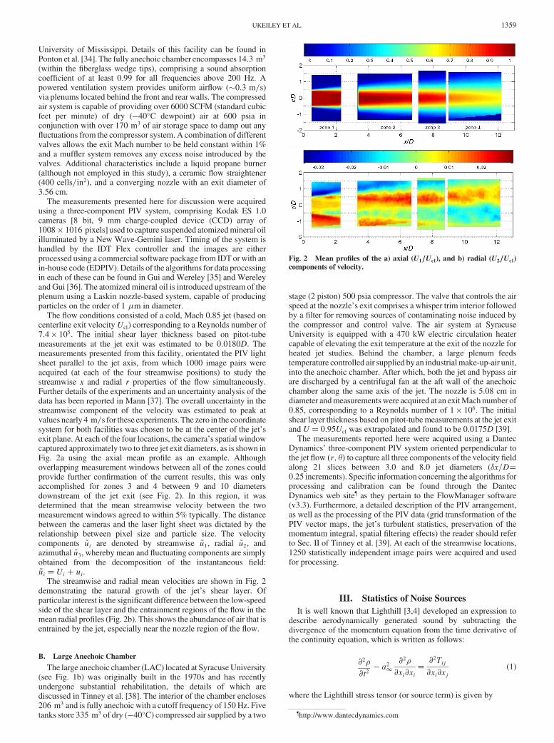
The flow conditions consisted of a cold, Mach 0.85 jet (based oncenterline exit velocityUcl) corresponding to a Reynolds number of7:4 � 105. The initial shear layer thickness based on pitot-tubemeasurements at the jet exit was estimated to be 0:0180D. Themeasurements presented from this facility, orientated the PIV lightsheet parallel to the jet axis, from which 1000 image pairs wereacquired (at each of the four streamwise positions) to study thestreamwise x and radial r properties of the flow simultaneously.Further details of the experiments and an uncertainty analysis of thedata has been reported in Mann [37]. The overall uncertainty in thestreamwise component of the velocity was estimated to peak atvalues nearly 4 m=s for these experiments. The zero in the coordinatesystem for both facilities was chosen to be at the center of the jet’sexit plane. At each of the four locations, the camera’s spatial windowcaptured approximately two to three jet exit diameters, as is shown inFig. 2a using the axial mean profile as an example. Althoughoverlapping measurement windows between all of the zones couldprovide further confirmation of the current results, this was onlyaccomplished for zones 3 and 4 between 9 and 10 diametersdownstream of the jet exit (see Fig. 2). In this region, it wasdetermined that the mean streamwise velocity between the twomeasurement windows agreed to within 5% typically. The distancebetween the cameras and the laser light sheet was dictated by therelationship between pixel size and particle size. The velocitycomponents ~ui are denoted by streamwise ~u1, radial ~u2, andazimuthal ~u3, whereby mean and fluctuating components are simplyobtained from the decomposition of the instantaneous field:~ui �Ui � ui.The streamwise and radial mean velocities are shown in Fig. 2
demonstrating the natural growth of the jet’s shear layer. Ofparticular interest is the significant difference between the low-speedside of the shear layer and the entrainment regions of the flow in themean radial profiles (Fig. 2b). This shows the abundance of air that isentrained by the jet, especially near the nozzle region of the flow.
B. Large Anechoic Chamber
The large anechoic chamber (LAC) located at SyracuseUniversity(see Fig. 1b) was originally built in the 1970s and has recentlyundergone substantial rehabilitation, the details of which arediscussed in Tinney et al. [38]. The interior of the chamber encloses206 m3 and is fully anechoic with a cutoff frequency of 150 Hz. Fivetanks store 335 m3 of dry (�40�C) compressed air supplied by a two
stage (2 piston) 500 psia compressor. The valve that controls the airspeed at the nozzle’s exit comprises a whisper trim interior followedby a filter for removing sources of contaminating noise induced bythe compressor and control valve. The air system at SyracuseUniversity is equipped with a 470 kW electric circulation heatercapable of elevating the exit temperature at the exit of the nozzle forheated jet studies. Behind the chamber, a large plenum feedstemperature controlled air supplied by an industrialmake-up-air unit,into the anechoic chamber. After which, both the jet and bypass airare discharged by a centrifugal fan at the aft wall of the anechoicchamber along the same axis of the jet. The nozzle is 5.08 cm indiameter andmeasurementswere acquired at an exitMach number of0.85, corresponding to a Reynolds number of 1 � 106. The initialshear layer thickness based on pitot-tubemeasurements at the jet exitand U� 0:95Ucl was extrapolated and found to be 0:0175D [39].
The measurements reported here were acquired using a DantecDynamics’ three-component PIV system oriented perpendicular tothe jet flow �r; �� to capture all three components of the velocity fieldalong 21 slices between 3.0 and 8.0 jet diameters (�x=D�0:25 increments). Specific information concerning the algorithms forprocessing and calibration can be found through the DantecDynamics web site¶ as they pertain to the FlowManager software(v3.3). Furthermore, a detailed description of the PIV arrangement,as well as the processing of the PIV data (grid transformation of thePIV vector maps, the jet’s turbulent statistics, preservation of themomentum integral, spatial filtering effects) the reader should referto Sec. II of Tinney et al. [39]. At each of the streamwise locations,1250 statistically independent image pairs were acquired and usedfor processing.
III. Statistics of Noise Sources
It is well known that Lighthill [3,4] developed an expression todescribe aerodynamically generated sound by subtracting thedivergence of the momentum equation from the time derivative ofthe continuity equation, which is written as follows:
@2�
@t2� a21
@2�
@xi@xi�@2Tij@xi@xj
(1)
where the Lighthill stress tensor (or source term) is given by
Fig. 2 Mean profiles of the a) axial (U1=Ucl), and b) radial (U2=Ucl)
components of velocity.
¶http://www.dantecdynamics.com
UKEILEY ET AL. 1359

Tij � � ~ui ~uj ��p � �a21
��ij � �ij (2)
Here, a1 is the ambient speed of sound and �ij is the viscous stresstensor. The left-hand side of this inhomogeneous wave, Eq. (1),represents the propagation of the sound after it leaves the turbulentflowfield, whereas the right-hand side is said to be representative ofthe generation of sound in the turbulent flow. Classically, the last twoterms on the right-hand side of the Lighthill stress tensor, Eq. (2), areneglected using a cold jet and high Reynold’s number assumptions,respectively, for each of the terms. Freund [10] recently evaluatedthese assumptions and showed that even in a lower Reynold’snumber jet, the contribution from the viscous stress tensor is indeednegligible. This, however, was not necessarily the case for themiddleterm. Because only the velocity field was acquired in the currentexperiments, we will work with the commonly used assumption thatTij � � ~ui ~uj.
The calculation of aerodynamically generated sound is conven-tionally carried out in one of two ways. The first involves directlyevaluating the source field on the right-hand side of Lighthill’sequations and using it as a time-dependent input in the solution ofEq. (1). This was carried out by Colonius&Freund [12] and requireda large computational effort not only to solve for the nonho-mogeneous wave equation, but to process a highly resolved grid thatwas necessary for adequately modeling the acoustic source terms.This is not possible using the current data set because it has beensampled discontinuously. However, Tinney et al. [40] havepresented amethod for reconstructing a time-resolved estimate of theflowfield through a mean-square estimation procedure. This tool hasdemonstrated many promising results and will be the subject offuture studies.
The second involves solving Eq. (1) for an analytical solution tothe density field. This has been shown previously for an unboundedflow and has the following form:
��y; t� 1
4�a21
ZZZV
1
jy � xj@2Tij�x; ��@xi@xj
dx (3)
where � is the density fluctuations in the far field and � is now aretarded time coefficient that is associatedwith the propagation of thesound. This can be rewritten as follows:
��y; t� 1
4�a41
xixjx3
ZZZV
@2Tij�x; ��@�2
dx (4)
where xi=x is the direction cosine between the source at x, and theobservation point at y. It should be pointed out that in much of theliterature on this subject, the direction cosines and Tij are combinedso that the equation is written with the second time derivative of Txxusing the velocity in the direction of the observation point. However,in instanceswhere PIV data are employed, itmay bemore convenientto leave it in the form shown in Eq. (4) because themeasurements aretypically acquired along a discretized Cartesian grid.
Typically, one is concerned with the far-field acoustic intensity,
I�y� � a31�oh��y; t�2i (5)
which, after substituting the density field ��x; t� in (5) using (4), wecan rewrite this as follows:
I�y� �xixjxkxl
16�2a51�ox4
ZV
ZV 0
�@2Tij@�2
@2T 0kl@�2
�dx dx0 (6)
Here, the first and second terms in the bracket are evaluated at (x; �)and (x0; �0) which are suitable retarded times to reach the observationpoint. Following the analysis of Proudman [41] and later, Ribner[42], the preceding relationship can be written as
I�y� �xixjxkxl
16�2a51�ox4
ZV
@4
@�4hTijT 0kli dr (7)
using several assumptions such as homogeneity of the turbulencefield. If one assumes that the only important term in the Lighthillstress tensor is the first, that is Tij � ~ui ~uj, then Eq. (7) can besimplified as
I�y� �xixjxkxk
16�2a51�ox4
ZV
@4
@�4h ~ui ~uj ~u0k ~u0li dr (8)
As one can see, the principle term in Eq. (8) comprises fourth-order, two-point, time and space correlations. Of course, other formsto the solution of the Lighthill equation can be derived if differentlimiting assumptions are applied, many of which result in the two-point correlation as the principle term.An example of this was shownby Seiner et al. [43] who used the properties from algebraiccorrelations to derive an expression for the far-field intensity. Thiswas obtained by multiplying the double divergence of a Green’sfunction with TijTkl, of which the former needed to be defined. Inconcert with Eq. (8), these formulations demonstrate the importancefor studying the two-point correlations as a means by which tounderstand and predict the noise sources in unbounded turbulentflows. In Secs. V and VI we will present the two-point spatialcorrelations from the data sets described in Sec. II.
IV. Single-Point Turbulent Statistics and the LighthillSource Term
If one is to solve the Lighthill equation, then one must be able tomeasure the source term Tij. The ability to measure all of the nineterms in this tensor, from which the double divergence is calculated,has been central to many of the complicating factors in studying thenoise sources generated by turbulence. Throughout the resultssections we will present turbulence properties as they relate to theLighthill source tensor.
First, we will examine some of the individual components of thesimplified form of Tij, i.e., uiuj using a subset of the data acquired atthe NCPA. The density term has been dropped here, and will beneglected throughout the Results section due to the lack of availablelocal density measurements. However, measurements of thestatistical quantities for the velocity have been found to closelyresemble hot-wire measurements (mass flux) in subsonic jets [23]where the static temperature and ambient conditions were matched.In Fig. 3a, the streamwise (top) and radial (bottom) components ofthe fluctuating velocity field are presented, normalized by the jet exitvelocity. The axial component is shown to peak between 8 and 10 jetdiameters at around 15%, whereas the radial component peaksaround 8%. Shear stress profiles of u1u2=U
2cl are also shown in
Fig. 3b with a peak around 0.7% of the jet exit velocity squared.These stress profiles agree well with the PIV measurements ofArakeri et al. [1] and Bridges [27], and in general show the samediscrepancies with the LDV measurements of Lau et al. [20], whichare attributed to the filtering effects inherent in PIVmeasurements asdescribed by Westerweel [44]. Centerline statistical features of theaxial velocity are shown in Fig. 3c whereby the potential core isshown to decay between five and six jet diameters. Arakeri et al. [1]showed that the mean axial velocity of a Mach 0.9 jet (D� 2:2 cm)decayed to 70% of the jet exit speed around x=D� 12, whereas thepeak in the axial rms occurred around 10 jet diameters. Likewise, thecenterline velocity of a Mach 0.6 jet (D� 8:2 cm) was shown todecay toward 60% by Narayanan et al. [45] with the axial rmsvelocity peaking similarly around 10 jet diameters. The currentmeasurements are complementary to these investigations wherebythe mean axial centerline velocity decays to roughly 65% of the jet’sexit velocity at x=D� 12 with a maximum in the turbulenceintensity at x=D� 10.
Figure 4 displays the components of the Reynolds stress tensorfrom the data acquired at the LAC in the (r–�) plane, normalized bythe jet exit velocity squared. The profiles are plotted using shear layercoordinates [��x� � �r � r0:5�=x]∗∗ and manifest linear growth
∗∗The radial location r0:5 is where the mean axial velocity is 50% of the jetexit velocity.
1360 UKEILEY ET AL.

patterns for the high- and low-speed sides of the shear layer wherebythe potential core is found to collapse between five and six jetdiameters, similar to the measurements shown in Fig. 3c of theNCPA jet. The axial stress profile shown in Fig. 4a demonstrates apeak around 1.8%, in concert with other reported findings [20],whereas the radial stresses are under at 0.8%. The azimuthalcomponent in Fig. 4c is slightly larger (0.9%) than the radialcomponent, although they are quite close in this data set, both ofwhich (radial and azimuthal) are nearly half the value of the axialcomponent, which overall, reflects the highly anisotropic nature ofthe turbulent jet. In concert with the shear stress term presented inFig. 3b from the NCPA jet, the shear stress term (axial–radial) inFig. 4d exhibits a peak around 0.7% of the jet exit velocity squared.The peak energy manifest on the high-speed side of the shear layer isin good agreement with the measurements of others [18,46]. Allnormal and shear stresses at x=D� 5 are shown in Fig. 4f,demonstrating that u1u2 is the only significantly nonzero componentof the shear stresses. The spatial correlations generated from the u1u3shear stress term will be subsequently presented as it should notnecessarily be discarded.
Where the peak energy is concerned, the spreading of the turbulentshear layer is visible in the normal components of the Reynoldsstresses where the levels at ��x� � 0 are shown to increase until thecollapse of the potential core, as was demonstrated by Narayananet al. [45]. Interestingly, the shear stress component u1u2 in Fig. 4ddoes not increase significantly, and maintains its profile well into thetransition region of the flow. In hindsight, the overall agreement ofthese two data sets to those presented in the literature demonstrates
the quality of the measurement techniques and of the facilitiesemployed to construct a natural turbulent jet.
V. Evolution of Two-Point Statistics
In this section, we will present two-point turbulent statisticsthroughout the measurement region and discuss the trends observedin the data. This will be done before evaluating the terms specific tothe Lighthill source tensor and is necessary to demonstrate thecharacteristics of the high Reynolds number transonic jet. Where theazimuthal extent of these two-point correlations are concerned, theazimuthal symmetry of the jet is considered, and the correlations areonlymapped over nonrepeating regions in space, that is between zeroand �. The mathematical form for calculating the normalizedcorrelations of the axial–radial and radial–azimuthal data is asfollows:
Rij�x; r� �hui�x; r; t�uj�x0; r0; t�i
hui�x; r; t�2i0:5huj�x0; r0; t�2i0:5
Rij�r; �� �hui�r; �; t�uj�r0; �0; t�i
hui�r; �; t�2i0:5huj�r0; �0; t�2i0:5
(9)
A. Streamwise Velocity
Starting with the measurements from the NCPA, the two-pointspatial correlations are evaluated across the jet’s streamwise andradial plane. The origins of these correlations are fixed at three pointsin the radial direction (r=D� 0:0, 0.5, and 0.74) and two axialpositions (x=D� 4:0 and x=D� 8:0), as shown in Figs. 5a and 5b,respectively.†† At r=D� 0:5, the axial extent of the streamwisecorrelation increases from nearly 0.5 jet diameters at x=D� 4, toapproximately one full jet diameter at x=D� 8. With the exceptionof regions within the potential core of the jet (r=D� 0:0), thestreamwise domain over which the correlated region extends is about2.5 times that of the radial domain. Where the radial extension ofthese correlations are concerned, they are shown to grow with theexpanding shear layer but do not extend over the entire shear layer, inview of the radial correlations shown next. One interesting feature inthis figure is the inclined nature of the correlation function in theshear layer regions of the flow, relative to the axis of the jet. This isalso seen in the measurements of Arakeri et al. [1] and can beattributed to the straining of the large-scale turbulence structure.
The azimuthal dependence of these correlations are demonstratedin Fig. 6, consistent with the transonic jet measurements (hot wires)of Ukeiley and Seiner [23] and the incompressible jet measurementsof Jung et al. [47]. Comparing the top (x=D� 4) and bottom(x=D� 8) profiles, the azimuthal extent of the streamwise spatialcorrelations in the outer part of themixing layer at x=D� 8 aremuchlarger when compared with the measurements observed at x=D� 4.The opposite is true in the potential core region where the correlatedregion has a larger azimuthal distribution at the upstream position.This is a well-known artifact of jet flows whereby the potential coreregion gives way to the expanding turbulent shear layer up until thecollapse of the potential core.
B. Radial Velocity
For the radial component of the two-point correlations (Fig. 7), thestreamwise extent of the large-scale structure does not exhibit thesame inclined behavior as the streamwise correlations (Fig. 5) andgrows at a fairly uniform rate in this region of the flow. A moreinteresting feature is the radial extent of the correlation in thepotential core region of the flow at r=R� 0:0 in Fig. 7a and 7b. Theaxial extent of this correlation is shown to have a spatial phase shift(in sign) of approximately one jet diameter at both x=D� 4 and 8,and is evidence of a compact well-organized flappingmode structure(a helical Fourier mode 1). This is consistent at both axial positions
Fig. 3 Stress profiles: a) velocity profiles of the axial (top) and radial
(bottom) stresses; b) shear stress hu1u2i=U2cl; and c) streamwise variation
of the axial velocity’s mean and turbulence intensity on the centerline
where u01 has been normalized by its maximum value and is thus
nondimensional.
††The origin for evaluating the correlations over the axial and radial planewill be the same in subsequent figures using the NCPA jet data with contourlevels ranging between �0:5 and 1.0 with increments of 0.1.
UKEILEY ET AL. 1361

shown. In the shear layer region (r=D� 0:5 and 0.74) at x=D� 8:0,the spatial extent of the correlation stretches to nearly one full jetdiameter, from about half a jet diameter at x=D� 4:0. As one mightexpect, the radial component of the large-scale structures convectingthrough the shear layer accounts for more of the shear layer’s growththan do the axial components.
Because the distribution of the radial correlations in the (r–x)plane (Fig. 7) demonstrate helical-type structures in the potentialcore regions of the flow, then the same should be expected of the
radial correlations across the (r–�) plane. Considering first that in acylindrical coordinate system, defined in a way that �r and �r(where r=D is positive) represent fluidmovements from the potentialcore to the shear layer and from the shear layer to the potential core,‡‡
respectively, then for a helical-type structure, the radial componentof the velocity vector should be opposite in sign for azimuthal
−0.1 −0.05 0 0.05 0.1 0.15 0.20
5
10
15
20
η(x)
<u 1u 1>
/Ucl2
× 10
3
4.0D4.5D5.0D5.5D6.0D6.5D7.0D7.5D8.0D
−0.1 −0.05 0 0.05 0.1 0.15 0.2
0
2
4
6
8
10
12
η(x)
<u 2u 2>
/Ucl2
× 10
3
−0.1 −0.05 0 0.05 0.1 0.15 0.2
0
2
4
6
8
10
12
η(x)
<u 3u 3>
/Ucl2
× 10
3
−0.1 −0.05 0 0.05 0.1 0.15 0.2
0
2
4
6
8
η(x)
<u 1u 2>
/Ucl2
× 10
3
−0.1 −0.05 0 0.05 0.1 0.15 0.20
5
10
15
20
η(x)
TK
E/U
cl2×
103
−0.1 −0.05 0 0.05 0.1 0.15 0.20
5
10
15
20
η(x)
<u iu j>
/Ucl2
× 10
3
i=1,j=1i=2,j=2i=3,j=3i=1,j=2i=1,j=3i=2,j=3
a)
d)
b)
e)
c)
f)
Fig. 4 Radial distribution of individual Reynolds stress components: a) axial i; j� 1, b) radial i; j� 2; c) azimuthal i; j� 3; d) shear i� 1, j� 2;
e) turbulent kinetic energy 0:5hu21 � u2
2 � u23i; and f) survey of Reynolds stress components at x=D� 5.
r/D = 0.0 r/D = 0 .5 r/D = 0 .74
3.5 4 4.5 5 5.5 6 6.5−1.5
−1
−0.5
0
0.5
1
1.5
x/D
r/D
3.5 4 4.5 5 5.5 6 6.5−1.5
−1
−0.5
0
0.5
1
1.5
x/D
r/D
0
0.2
0.4
0.6
0.8
3.5 4 4.5 5 5.5 6 6.5−1.5
−1
−0.5
0
0.5
1
1.5
x/D
r/D
7 7.5 8 8.5 9 9.5 10−1.5
−1
−0.5
0
0.5
1
1.5
x/D
r/D
7 7.5 8 8.5 9 9.5 10−1.5
−1
−0.5
0
0.5
1
1.5
x/D
r/D
0
0.2
0.4
0.6
0.8
7 7.5 8 8.5 9 9.5 10−1.5
−1
−0.5
0
0.5
1
1.5
x/D
r/D
a)
b)
−0.2
−0.4
−0.5
−0.2
−0.4
−0.5
Fig. 5 Normalized streamwise velocity correlation coefficients in the (r–x) plane at a) x=D� 4:0, and b) x=D� 8:0.
‡‡The opposite being true for the section of the jet where r=D is negative.
1362 UKEILEY ET AL.

separations 180 deg away from the point of origin. This is indeed thecase as is shown in Fig. 8 at r=D� 0:03where the radial extent of theradial correlation is opposite in sign with respect to the diametricdisposition of the point of origin. The Fourier–azimuthaldecomposition of the Mach 0.85 jet has been performed by Tinney
et al. [33] using the correlations presented here and demonstrated asignificant contribution to the turbulent energy from the helical modestructure at these Reynolds numbers and jet exit speeds whencompared with the lower speed, lower Reynolds number flowspresented by Jung et al. [47].
r/D = 0.03 r/D = 0.5 r/D = 0.75
−0.1
0
0.1
0.2
0.3
0.4
0.5
0.6
0.7
0.8
0.9
−1.5 −1 −0.5 0 0.5 1 1.5
−1.5
−1
−0.5
0
0.5
1
1.5
r/D
r/D
−0.1
0
0.1
0.2
0.3
0.4
0.5
0.6
0.7
0.8
−1.5 −1 −0.5 0 0.5 1 1.5
−1.5
−1
−0.5
0
0.5
1
1.5
r/D
r/D
−0.1
0
0.1
0.2
0.3
0.4
0.5
0.6
0.7
0.8
−1.5 −1 −0.5 0 0.5 1 1.5
−1.5
−1
−0.5
0
0.5
1
1.5
r/D
r/D
Fig. 6 Normalized streamwise velocity correlation coefficients in the (r–�) plane at x=D� 4 (top) and x=D� 8 (bottom).
r/D = 0.0 r/D = 0.5 r/D = 0.74
3.5 4 4.5 5 5.5 6 6.5−1.5
−1
−0.5
0
0.5
1
1.5
x/D
r/D
3.5 4 4.5 5 5.5 6 6.5−1.5
−1
−0.5
0
0.5
1
1.5
x/D
r/D
0
0.2
0.4
0.6
0.8
3.5 4 4.5 5 5.5 6 6.5−1.5
−1
−0.5
0
0.5
1
1.5
x/Dr/
D
7 7.5 8 8.5 9 9.5 10−1.5
−1
−0.5
0
0.5
1
1.5
x/D
r/D
7 7.5 8 8.5 9 9.5 10−1.5
−1
−0.5
0
0.5
1
1.5
x/D
r/D
0
0.2
0.4
0.6
0.8
7 7.5 8 8.5 9 9.5 10−1.5
−1
−0.5
0
0.5
1
1.5
x/D
r/D
−0.2
−0.4
−0.5
−0.2
−0.4
−0.5
a)
b)
Fig. 7 Normalized radial velocity correlation coefficients in the (r–x) plane at a) x=D� 4:0, and b) x=D� 8:0.
r/D = 0.03 r/D = 0.5 r/D = 0.75
−0.8
−0.6
−0.4
−0.2
0
0.2
0.4
0.6
0.8
−1.5 −1 −0.5 0 0.5 1 1.5
−1.5
−1
−0.5
0
0.5
1
1.5
r/D
r/D
−0.1
0
0.1
0.2
0.3
0.4
0.5
0.6
0.7
0.8
0.9
−1.5 −1 −0.5 0 0.5 1 1.5
−1.5
−1
−0.5
0
0.5
1
1.5
r/D
r/D
−0.1
0
0.1
0.2
0.3
0.4
0.5
0.6
0.7
0.8
0.9
−1.5 −1 −0.5 0 0.5 1 1.5
−1.5
−1
−0.5
0
0.5
1
1.5
r/D
r/D
Fig. 8 Normalized radial velocity correlation coefficients in the (r–�) plane at x=D� 4 (top) and x=D� 8 (bottom).
UKEILEY ET AL. 1363

At r=D� 0:5 and 0.75 in Fig. 8 (where the points of origin arewithin the shear layer regions), the spatial extent of the correlationsare shown to grow more in the radial direction than in the azimuthaldirection where the differences in the downstream position areconcerned. This small growth (azimuthally) results in the presence ofhigher Fourier–azimuthal modes that are commonly found in thelow-speed (low-frequency) side of the turbulent jet’s shear layer[23].
C. Azimuthal Velocity
In light of the aforementioned normal stresses, the (r–x) spatialdistribution of the azimuthal correlation (Fig. 9) demonstrates avector component of the large-scale turbulent structurewhich ismorecompact and less dispersive in space. Similar to the axial correlationsshown in Fig. 5, the azimuthal correlations are inclined at an anglewhich appears to be around 20–30 deg from the jet axis (dashed line),however, it is much more pronounced here. This is an interestingartifact considering that the peak radiation of the pressure field thatpropagates into the far field has been shown to typically occur at anangle of 20–30 deg from the positive jet axis. Furthermore, theobliqueness of the correlation appears to have little dependence onthe axial or radial position in the flow in view of themeasurements in
Figs. 9a and 9b.One interpretation of this behavior exhibited by thesecorrelations is due to a helical structure associated with the azimuthalvelocity. For origins on the centerline of the jet, there is a largecorrelated region which extends equally in the radial and streamwisedirections while exhibiting features of an oblique structure in theshear layer. This behavior appears to be consistent throughout theentire streamwise domain studied.
The azimuthal extent of the azimuthal correlations are shown inFig. 10 and are similar to the radial velocity correlations atr=D� 0:0, whereby the sign switching articulates the presence of ahelical azimuthal mode structure in the potential core regions. Theradial extent of these correlations are nearly half of those observed forthe radial velocity. In the mixing layer, the spatial extension of thecorrelation azimuthally is similar to the (r–x) distribution of theradial correlations illustrated in Fig. 7, thus demonstrating how theenergy shifts to lower Fourier–azimuthalmode numbers after the endof the potential core [24].
D. Shear Components
Although we have only considered so far the two-pointcorrelations of the normal stresses, the shear stress components of thevelocity field are presented here for completeness. In Fig. 11, the
r/D = 0.0 r/D = 0.5 r/D = 0.74
3.5 4 4.5 5 5.5 6 6.5−1.5
−1
−0.5
0
0.5
1
1.5
x/D
r/D
3.5 4 4.5 5 5.5 6 6.5−1.5
−1
−0.5
0
0.5
1
1.5
x/D
r/D
−0.5
−0.4
−0.2
0
0.2
0.4
0.6
0.8
3.5 4 4.5 5 5.5 6 6.5−1.5
−1
−0.5
0
0.5
1
1.5
x/D
r/D
7 7.5 8 8.5 9 9.5 10−1.5
−1
−0.5
0
0.5
1
1.5
x/D
r/D
7 7.5 8 8.5 9 9.5 10−1.5
−1
−0.5
0
0.5
1
1.5
x/D
r/D
0
0.2
0.4
0.6
0.8
7 7.5 8 8.5 9 9.5 10−1.5
−1
−0.5
0
0.5
1
1.5
x/D
r/D
a)
b)
−0.4
−0.2
−0.5
Fig. 9 Normalized azimuthal velocity correlation coefficients in the (r–x) plane at a) x=D� 4:0, and b) x=D� 8:0.
r/D = 0.03 r/D = 0.5 r/D = 0.75
−0.8
−0.6
−0.4
−0.2
0
0.2
0.4
0.6
0.8
−1.5 −1 −0.5 0 0.5 1 1.5
−1.5
−1
−0.5
0
0.5
1
1.5
r/D
r/D
−0.1
0
0.1
0.2
0.3
0.4
0.5
0.6
0.7
0.8
0.9
−1.5 −1 −0.5 0 0.5 1 1.5
−1.5
−1
−0.5
0
0.5
1
1.5
r/D
r/D
−0.2
−0.1
0
0.1
0.2
0.3
0.4
0.5
0.6
0.7
0.8
−1.5 −1 −0.5 0 0.5 1 1.5
−1.5
−1
−0.5
0
0.5
1
1.5
r/D
r/D
Fig. 10 Normalized azimuthal velocity correlation coefficients in the (r–�) plane at x=D� 4 (top) and x=D� 8 (bottom).
1364 UKEILEY ET AL.

u1u2 components illustrate similar characteristics to the radialcorrelations (Fig. 7) in the shear layer regions of the flow. Thecorrelations at the jet’s center (r=D� 0:0) show evidence of fluidbeing entrained before the point of origin, followed by an ejection offluid from the potential core after the point of origin. The spatialseparation between these events are on the order of one jet diameter atboth axial stations, and is consistent with streamwise and radialcorrelations shown in Figs. 5 and 7. It should be noted that the sign ofthese correlations is an artifact of the coordinate system and that the
relationship of the axial–radial shear stresses agree with the generaltheorem that uv���T�@U=@r�.
The same phenomena is shown in Fig. 12a at r=D� 0:03,whereby the potential core region of the flow manifests a strongazimuthal correlation resulting from the passage of turbulentstructures whose radial and axial components are phase aligned. Thishas been demonstrated by Citriniti &George [48] who reconstructedtime-resolved slices through the (r–�) plane of the low-Reynoldsnumber, low-speed jet and the eruption of highly correlated
r/D = 0.0 r/D = 0.5 r/D = 0.74
−0.5
−0.4
−0.3
−0.2
−0.1
0
0.1
0.2
3.5 4 4.5 5 5.5 6 6.5−1.5
−1
−0.5
0
0.5
1
1.5
x/D
r/D
−0.5
−0.4
−0.3
−0.2
−0.1
0
0.1
0.2
0.3
0.4
0.5
3.5 4 4.5 5 5.5 6 6.5−1.5
−1
−0.5
0
0.5
1
1.5
x/D
r/D
−0.5
−0.4
−0.3
−0.2
−0.1
0
0.1
0.2
0.3
0.4
0.5
3.5 4 4.5 5 5.5 6 6.5−1.5
−1
−0.5
0
0.5
1
1.5
x/D
r/D
0
0.1
7 7.5 8 8.5 9 9.5 10−1.5
−1
−0.5
0
0.5
1
1.5
x/D
r/D
0
0.1
0.2
0.3
0.4
0.5
7 7.5 8 8.5 9 9.5 10−1.5
−1
−0.5
0
0.5
1
1.5
x/D
r/D
0
0.1
0.2
0.3
0.4
0.5
7 7.5 8 8.5 9 9.5 10−1.5
−1
−0.5
0
0.5
1
1.5
x/D
r/D
a)
b)
−0.5
−0.4
−0.3
−0.2
−0.1
−0.5
−0.4
−0.3
−0.2
−0.1
−0.5
−0.4
−0.3
−0.2
−0.1
Fig. 11 Normalized shear velocity correlation coefficients in the (r–x) plane at a) x=D� 4:0, and b) x=D� 8:0.
r/D = 0.03 r/D = 0.5 r/D = 0.75
−0.15
−0.1
−0.05
0
0.05
0.1
−1.5 −1 −0.5 0 0.5 1 1.5
−1.5
−1
−0.5
0
0.5
1
1.5
r/D
r/D
−0.1
0
0.1
0.2
0.3
0.4
0.5
−1.5 −1 −0.5 0 0.5 1 1.5
−1.5
−1
−0.5
0
0.5
1
1.5
r/D
r/D
−0.1
0
0.1
0.2
0.3
0.4
−1.5 −1 −0.5 0 0.5 1 1.5
−1.5
−1
−0.5
0
0.5
1
1.5
r/D
r/D
−0.06
−0.04
−0.02
0
0.02
0.04
0.06
−1.5 −1 −0.5 0 0.5 1 1.5
−1.5
−1
−0.5
0
0.5
1
1.5
r/D
r/D 0
0.05
0.1
0.15
0.2
0.25
−1.5 −1 −0.5 0 0.5 1 1.5
−1.5
−1
−0.5
0
0.5
1
1.5
−0.2
r/D
r/D
−0.2
−0.1
0
0.05
0.1
0.15
0.2
0.25
−1.5 −1 −0.5 0 0.5 1 1.5
−1.5
−1
−0.5
0
0.5
1
1.5
r/D
r/D
a)
b)
−0.05
−0.1
−0.15
−0.25
−0.05
−0.15
Fig. 12 Normalized shear velocity correlation coefficients in the (r–�) plane at x=D� 4 (top) and x=D� 8 (bottom) for a) (u1u2), and b) (u1u3).
UKEILEY ET AL. 1365

structures through the flow’s potential core regions followed byhigher Fourier mode events in the low-speed side of the shear layer[49].
Figure 12b displays the streamwise–azimuthal velocitycorrelations in the (r–�) plane. One can see that the correlationbetween these two components is weak in the potential core region,but should not be so easily discarded in the shear layer regions as theyappear to possess a fair percentage of the total turbulent velocity’senergy. The fact that both of these correlations exhibitedantisymmetric patterns implies that when the spatial volumes areintegrated in Lighthill’s analysis, these components will notcontribute (or very little) when there is no time separation. Thisdemonstrates the necessity for evaluating the space-time character-istics of these correlations to determine whether these eventscontribute significantly to the radiated noise field.
VI. Quadrupole Correlations
To calculate the relative contributions of the different quadrupoleself- and cross-correlations to the sound emitted in a given direction,Ribner [42] reformulated the Lighthill theory by postulatingisotropic turbulence superposed on amean flow. This is important, asthe effects of convection and refraction, which are known todominate the heart-shaped pattern of jet noise, can be corrected out toyield the small basic directivity of the eddy noise generators [42].
The process entails reducing the 36 possible quadrupolecorrelations to a distinct set of nine, nonvanishing correlationintegrals, shown in Eq. (8) as h ~ui ~uj ~u0k ~u0li, that contribute to theaxisymmetric noise pattern of a round jet. Decomposing the instan-taneous field into mean and turbulence quantities ( ~ui �Ui � ui),leads to the terms commonly known as “shear” and “self” noisecomponents. The shear-noise (fast) components compriseinteractions of the mean flow with the turbulence, UiU
0jhuku0li,
whereas the self-noise (slow) components involve interactions of theturbulence with the turbulence huiuju0ku0li. Note that the primes inRibner’s formulation [42] comprise velocity terms that are functionsof both spatial and temporal separations. With the current data set,only spatial separations can be examined. In the absence of temporalinformation, this may be misleading because the latter of the twodemonstrates the frequency dependence of the space-time structure.However, one can still gain insight into the relative weights of thecomponents by examining these correlations with spatial separationsonly, and in addition, this information can serve to help guide futureanalysis.
In the subsequent discussion, the nine different source terms willbe analyzed to provide a basic understanding of their relativecontribution to the overall noise generated by round jets.Whereas thespatial correlations have been shown to comprise inhomogeneousand anisotropic behavior, the evaluation of Ribner’s terms are stillexact. It is worth mentioning that the effects of the isotropicassumption are being evaluated by many such as Khavrahan [17],Seiner et al. [43], and Jordan and Gervais [18]. The measurements inthe latter two studies mentioned have shown that using the isotropicassumptions overestimate the shear-noise terms and that the self-noise terms dominate shear-noise terms by up to a factor of 2.5 whenthe anisotropic shape of the jet structure is retained. Thus, by directlycalculating these terms from the PIV measurement, one is able toneglect any assumptions that may be otherwise limiting anddemonstrate their true spatial topology.
A. Shear-Noise Terms
In the axisymmetric jet, the mean streamwise velocity is at leastone order of magnitude greater than the radial or azimuthal velocities(Fig. 2). Therefore, the only significant shear-noise terms would be
U1U01hu1u01i U1U
01hu2u02i U1U
01hu3u03i (10)
Clearly, these terms will have similar behavior to what wasdiscussed in the previous section where the two-point statistics areconcerned and are illustrated in Fig. 13 using the r–x plane data at
x=D� 4. These shear-noise terms are normalized by U4cl and the
radial position of the origin is identified at the top of each column.One can see from Fig. 13 that the azimuthal component
(U1U01hu3u03i) comprises the strongest correlation in all regions of the
flow, except in the low-speed side of the shear layer (r=D� 0:75)where the azimuthal and streamwise correlations are maximallysimilar. It is interesting to point out that where the radial dependenceof the origin is concerned, the correlations shown in Fig. 13 weredetermined to comprise the greatest levels using the origins atr=D� 0:33. Thus, the maximum shear-noise correlations(determined for all three components) are favorable toward thehigh-speed side of the shear layer. The significance of this, where thepressure field is concerned, has been investigated recently by Hallet al. [50] whereby the near-field pressure region surrounding a high-speed subsonic jet flow has been found to have a strong lineardependence, hpui, with the velocity field along the interfacial regionof the flow between the potential core and the high-speed side of theshear layer. The same pressure velocity correlationswere extended toquadratic relationships by Tinney et al. [40] to quantify the nonlineardependencies, hpuui. The results exhibited identical spatialdependencies between the linear and nonlinear correlations,although the linear term was shown to contain higher levels than thenonlinear term. Therefore, the findings reported here demonstrateimportant information concerning the near-field pressure andperhaps insight into the noise generating events of the flow. Theshear-noise terms, with origins located further downstream (notshown),were quite similar to those shownhere at x=D� 4; themajordifferences being slightly higher values over a slightly larger area.
B. Self-Noise Terms
The last surviving self-noise terms (nine) that contribute to thenoise pattern of the jet are written as follows:
Du21u
021
E Du21u
022
E Du1u2u
01u02
E Du22u
022
E Du21u
023
EDu1u3u
01u03
E Du23u
023
E Du22u
023
E Du2u3u
02u03
E(11)
The spatial distribution of a subset of these correlations are shown inFig. 14 at x=D� 4 and, in general, have smaller peak values than theshear-noise terms. Like the shear-noise terms, the origin in the radialdirection was selected based on the maximum correlation valuewhich was found to follow the lip-line of the jet at r=D� 0:5. This isdifferent from the shear-noise terms (Fig. 13) whereby themaximumcorrelation was found to occur on the high-speed side of the mixinglayer. For the self-noise terms, the normal stress correlations hu21u023 iand hu22u023 i were similar to the hu21u022 i correlation in Fig. 14, and soare not shown. Also, the spatial distribution of the shear stresscorrelation hu2u3u02u03i (not shown) was similar to the shear stresscorrelation hu1u3u01u03i, although the latter of the two (shown inFig. 14) contained a peak value of nearly twice that of the former.One can see from these correlations that, except for the shear stressterm hu1u3u01u03i (and hence hu2u3u02u03i), the correlations extend tothe opposite side of the mixing layer. By comparing the relativeamplitudes of these functions, it is clear that the dominant self-noiseterms for the zero time delay case are the axial hu21u021 i and azimuthalhu23u023 i normal stresses.
VII. Summary
The turbulent statistics as they relate to the Lighthill source termswere investigated in a high Reynolds number, Mach 0.85axisymmetric jet flow. Specifically, the two-point spatial statisticswere studied to determine trends in all three flow coordinates. Theanalysis comprised measurements from two separate experimentsusing stereo three-component PIV techniques, that is, one with thelight sheet orientated in the streamwise direction (r–x) and one withthe light sheet orientated perpendicular to the jet flow (r–�). Thesingle-point statistics were in good agreement with previouslymeasured flow quantities and demonstrated typical inhomogeneous
1366 UKEILEY ET AL.

and anisotropic behaviors of high-speed, high Reynolds number,subsonic jet flows.
Two-point statistics were also presented and illustrated the largespatial coherence in the potential core regions of the flow where thelow-order structures of the flow are known to persist, whereas theazimuthal spatial correlations in the mixing layer regionsdemonstrated the characteristics that are typical of higher modenumber (Fourier–azimuthal) events. A full vector decomposition ofthe velocity field was performed by Tinney et al. [33] and
demonstrated that this is indeed the case, as has been shown by otherinvestigators [24,47]. Where the axial and radial spatial dependenceof the normal stresses are concerned, the axial and azimuthalcomponents of velocity demonstrated an oblique-shaped structure inthe mixing layer regions of the flow, whereas the radial normalstresses evolved downstream more uniformly.
Quadrupole correlations were also presented to demonstrate theirspatial evolution in the radial and streamwise directions. From this,the peak energy for the shear-noise component at x=D� 4was found
u21u 2
1 u22u 2
2 u23u 2
3
2
4
6
8
10
12x 10
−4
4 5 6
−1
−0.5
0
0.5
1
x/D
r/D
0
0.2
0.4
0.6
0.8
1
1.2
x 10−4
4 5 6
−1
−0.5
0
0.5
1
x/D
r/D
0
0.5
1
1.5
2
x 10−3
4 5 6
−1
−0.5
0
0.5
1
x/D
r/D
u21u 2
2 u1u2u1u2 u1u3u1u3
0
1
2
x 10−4
4 5 6
−1
−0.5
0
0.5
1
x/D
r/D
−1.5
−1
−0.5
0
0.5
1
1.5
2x 10
−4
4 5 6
−1
−0.5
0
0.5
1
x/D
r/D
0
1
2
3
4
5
x 10−4
4 5 6
−1
−0.5
0
0.5
1
x/D
r/D
Fig. 14 Self-noise spatial correlations normalized by U4cl in the (r–x) plane, with the origin located at x=D� 4 and r=D� 0:5.
r/D = 0.0 r/D = 0.33 r/D = 0.75
−5
0
5
10x 10
−4
4 5 6
−1
−0.5
0
0.5
1
x/D
r/D
0
2
4
6
8
10x 10
−3
4 5 6
−1
−0.5
0
0.5
1
x/D
−2
−1
0
1
2
3
4
5
x 10−4
4 5 6
−1
−0.5
0
0.5
1
x/D
−6
−4
−2
0
2
4
6
8
10
12x 10
−4
4 5 6
−1
−0.5
0
0.5
1
x/D
−1
−0.5
0
0.5
1
1.5
2
2.5
3
x 10−3
4 5 6
−1
−0.5
0
0.5
1
x/D
−1.5
−1
−0.5
0
0.5
1
1.5
2x 10
−4
4 5 6
−1
−0.5
0
0.5
1
x/D
−1
−0.5
0
0.5
1
1.5
2
x 10−3
4 5 6
−1
−0.5
0
0.5
1
x/D
−2
0
2
4
6
8
10
12
x 10−3
4 5 6
−1
−0.5
0
0.5
1
x/D
−4
−3
−2
−1
0
1
2
3
4
5x 10
−4
4 5 6
−1
−0.5
0
0.5
1
x/D
r/D
r/D
r/D
r/D r/D
r/D
r/D
r/D
a)
b)
c)
Fig. 13 Shear-noise spatial correlations for a) streamwise U1U01hu1u
01i, b) radial U1U
01hu2u
02i, and c) azimuthal U1U
01hu3u
03i components of velocity.
UKEILEY ET AL. 1367

to reside on the high-speed side of the shear layer aroundr=D� 0:33, whereas the self-noise terms peaked along the lip-line atr=D� 0:5. Coincidentally, the axial hu21u021 i and azimuthal hu23u023 inormal stresses, and the combined normal stress term hu21u023 icomprised significantly greater correlation levels than all of the othernine self-noise terms.
Although this analysis has shed some insight into the noise sourcesin transonic jets following Ribner [42], space and time information isnecessary to establish the link to the far-field noise. In this vane,conditional estimation techniques have been developed inconjunction with low-dimensional techniques [33,40] to permittime-resolved reconstructions of the jet’s three-dimensional, large-scale structure. From this, the time dependence of the variousquadrupole source terms can be calculated and the mechanismsresponsible for jet noise can be assessed more thoroughly.
Acknowledgments
This work has been partially funded by a grant from Air ForceOffice of Scientific Research, J. Schmisseur, technical monitor. Theauthors would also like to thank B. Jansen, R. Danforth, N. Murray,and L. Gui for assistance in acquiring and processing the particleimaging velocimetrymeasurements at the Jamie L.Whitten NationalCenter for Physical Acoustics facility.
References
[1] Arakeri, L., Krothapalli, A., Siddavaram, V., Alkislar, M. B., andLourenco, L. M., “On the use of Microjets to Suppress Turbulence in aMach 0.9 Axisymmetric Jet,” Journal of Fluid Mechanics, Vol. 490,Aug. 2003, pp. 75–98.
[2] Freund, J. B., “Noise Sources in a Low-ReynoldsNumber Turbulent Jetat Mach 0.9,” Journal of Fluid Mechanics, Vol. 438, July 2001,pp. 277–305.
[3] Lighthill, M. J., “On Sound Generated Aerodynamically 1: GeneralTheory,” Proceedings of the Royal Society of London, Series A:
Mathematical and Physical Sciences, Vol. 211, March 1952, pp. 564–587.
[4] Lighthill, M. J., “On Sound Generated Aerodynamically 2: Turbulenceas a Source of Sound,” Proceedings of the Royal Society of London,
Series A: Mathematical and Physical Sciences, Vol. 222, Feb. 1954,pp. 1–32.
[5] Crighton, D. G., “Basic Principals of Aerodynamic Noise Generation,”Progress in Aerospace Sciences, Vol. 16, No. 1, 1975, pp. 31–96.
[6] Ffowcs–Williams, J. E., “Aeroacoustics,” Annual Review of Fluid
Mechanics, Vol. 9, 1977, pp. 447–468.[7] Goldstein, M. E., Aeroacoustics, McGraw–Hill, New York, 1976.[8] Ribner, H. S., “Perspectives on Jet Noise,” AIAA Journal, Vol. 19,
No. 12, 1981, pp. 1513–1526.[9] Lilley, G. M., Jet Noise: Classical Theory and Experiments, edited by
H. Hubbard, Vol. 1, NASA Reference Publ. 1258, 1991.[10] Freund, J. B., “Noise-Source Turbulent Statistics and the Noise from a
Mach 0.9 Jet,” Physics of Fluids, Vol. 15, No. 6, 2003, pp. 1788–1799.[11] Bogey, C., Bailly, C., and Juvé, D., “Noise Investigation of a High
Subsonic,Moderate Reynolds Number Jet Using a Compressible LargeEddy Simulation,” Theoretical and Computational Fluid Dynamics,Vol. 16, No. 4, 2003, pp. 273–297.
[12] Colonius, T., and Freund, J. B., “Application of Lighthill’s Equation toa Mach 1.92 Turbulent Jet,” AIAA Journal, Vol. 38, No. 2, 1999.
[13] Whitmire, J., and Sarkar, S., “Validation of Acoustic-AnalogyPredictions for Sound Radiated by Turbulence,” Physics of Fluids,Vol. 12, No. 2, 2000, pp. 381–391.
[14] Samanta, A., Freund, J. B., Wei, M., and Lele, S. K., “Robustness ofAcoustic Analogies,” AIAA Journal, Vol. 44, No. 11, 2006.
[15] Goldstein, M., “Generalized Acoustic Analogy,” Journal of Fluid
Mechanics, Vol. 488, Aug. 2003, pp. 315–333.[16] Lilley, G. M., “On the Noise from Jets,” AGARD CP-131, 1974.[17] Khavaran, A., “Role of Anisotropy in Turbulent Mixing Noise,” AIAA
Journal, Vol. 37, No. 7, 1999, pp. 832–842.[18] Jordan, P., and Gervais, Y., “Modelling Self- and Shear-Noise
Mechanisms in Inhomogeneous, Anisotrpic Turbulence,” Journal of
Sound and Vibration, Vol. 279, Nos. 3–5, Jan. 2005, pp. 529–555.[19] Harper-Bourne, M., “Jet Noise Turbulence Measurments,” AIAA
Paper 03-3214, 2003.[20] Lau, J. C., Morris, P. J., and Fisher, M. J., “Measurements in Subsonic
and Supersonic Free Jets Using a Laser Velocimeter,” Journal of Fluid
Mechanics, Vol. 93, No. 1, 1979, pp. 1–27.[21] Morris, P. J., “Turbulence Measurements in Subsonic and Supersonic
Axisymmetric Jets in a Parallel Stream,” AIAA Journal, Vol. 14, No. 6,1976, pp. 1468–1475.
[22] Stromberg, J. L.,McLaughlin, D. K., and Troutt, T. R., “Flow Field andAcoustic Properties of a Mach Number 0.9 Jet at a Low ReynoldsNumber,” Journal of Sound and Vibration, Vol. 72, No. 2, 1980,pp. 159–176.
[23] Ukeiley, L., and Seiner, J., “Examination of Large Scale Structures in aTransonic Jet Mixing Layer,” ASME Paper FEDSM98-5234, 1998.
[24] Ukeiley, L., Seiner, J., and Ponton, M., “Azimuthal Structure of anAxisymmetric Jet Mixing Layer,” ASME Paper FEDSM99-7252,1999.
[25] Seiner, J., Ukeiley, L., and Ponton, M., “Jet Noise SourceMeasurements Using PIV,” AIAA Paper 99-1869, 1999.
[26] Bridges, J., andWernet,M., “Measurements of the Aeroacoustic SoundSource in Hot Jets,” AIAA Paper 03-3130, 2003.
[27] Bridges, J., “Effect of Heat on Space-Time Correlations in Jets,”AIAAPaper 06-2534, 2006.
[28] Siddon, T. E., “Noise Source Diagnostics Using CausalityCorrelations,” AGARD CP-131, 1973.
[29] Seiner, J. M., and Reethof, G., “On the Distribution of SourceCoherency in Subsonic Jets,” AIAA Paper 74-0004, 1974.
[30] Schaffar, M., “Direct Measurements of Axial Correlations in JetVelocity Fluctuations and Far Field Noise Near the Axis of Cold Jets,”Journal of Sound and Vibration, Vol. 64, No. 1, 1979, pp. 73–83.
[31] Juvé, D., Sunyach, M., and Comte-Bellot, G., “Intermittency of NoiseEmissions in Subsonic Cold Jets,” Journal of Sound and Vibration,Vol. 71, No. 3, 1980, pp. 319–332.
[32] Thurow, B., Hileman, J., Lempert, W., and Samimy, M., “Techniquefor Real-Time Visualization of Flow Structure in High-Speed Flows,”Physics of Fluids, Vol. 14, No. 10, Oct. 2002, pp. 3449–3552.
[33] Tinney, C. E., Ukeiley, L. S., and Glauser, M. N., “Evolution of theMost Energetic Modes in a High Sub-Sonic Mach Number TurbulentJet,” AIAA Paper 05-0417, Jan. 2005.
[34] Ponton, M. K., Seiner, J., Ukeiley, L., and Jansen, B., “New AnechoicChamber Design for Testing High Temperature Jet Flows,” AIAAPaper 01-2190, Jan. 2001.
[35] Gui, L., and Wereley, S., “Correlation Based Continuous Window-Shift Technique to Reduce the Peak-Locking Effect in Digital PIVImage Evaluation,” Experiments in Fluids, Vol. 32, No. 4, April 2002,pp. 506–517.
[36] Wereley, S., and Gui, L., “Correlation Based Central Difference ImageCorrection (CDIC) Method and Application in a Four-Roll Mill FlowPIV Measurement,” Experiments in Fluids, Vol. 34, No. 1, Jan. 2003,pp. 42–51.
[37] Mann, R., “Turbulence Properties of a Mach 0.85 Jet,” Ph.D.Dissertation, Univ. of Mississippi, University, MS, 2006.
[38] Tinney, C. E., Hall, A., Glauser,M.N.,Ukeiley, L. S., andCoughlin, T.,“Designing an Anechoic Chamber for the Experimental Study of HighSpeed Heated Jets,” AIAA Paper 04-0010, Jan. 2004.
[39] Tinney, C. E., Ukeiley, L. S., and Glauser, M. N., “Low-DimensionalCharacteristics of Subsonic Jet Flows,” Journal of Fluid Mechanics,pp. 1–28 (Currently in review).
[40] Tinney, C. E., Jordan, P., Hall, A. M., Delville, J., and Glauser, M. N.,“Time-Resolved Estimate of the Turbulence andSourceMechanisms ina Subsonic Jet Flow,” Journal of Turbulence, (to be published).
[41] Proudman, I., “Generation of Noise by Isotropic Turbulence,”Proceedings of the Royal Society of London, Series A: Mathematical
and Physical Sciences, Vol. 214, No. 1116, Aug. 1952, pp. 119–132.[42] Ribner, H. S., “Quadrupole Correlations Governing the Pattern of Jet
Noise,” Journal of Fluid Mechanics, Vol. 38, No. 1, Aug. 1969, pp. 1–24.
[43] Seiner, J., Ukeiley, L., Ponton, M., and Jansen, B. J., “Progress inExperimental Measure of Turbulent Flow for Aeroacoustics,” AIAAPaper 02-2402, 2002.
[44] Westerweel, J., “Effect of Sensor Geometry on the Performance of PIVInterrogation,” 9th International Symposium on Laser Techniques
Applied to Fluid Mechanics, Springer, Lisbon, Portugal, 1998, pp. 37–55.
[45] Narayanan, S., Barber, T., and Polak, D., “High Subsonic JetExperiments: Turbulence and Noise Generation Studies,” AIAA
Journal Vol. 40, 2003, pp. 430–437.[46] Hussain, A. K. M. F., and Clark, A. R., “On the Coherent Structure of
theAxisymmetricMixing Layer: a Flow-Visualization Study,” Journalof Fluid Mechanics, Vol. 104, 1981, pp. 263–294.
[47] Jung, D., Gamard, S., and George, W. K., “Downstream Evolution ofthe Most Energetic Modes in a Turbulent Axisymmetric Jet at HighReynolds Number, Part 1: the Near-Field Region,” Journal of Fluid
1368 UKEILEY ET AL.
Mechanics, Vol. 514, Sept. 2004, pp. 173–204.[48] Citriniti, J., and George, W., “Reconstruction of the Global Velocity
Field in the Axisymmetric Mixing Layer Using the Proper OrthogonalDecomposition,” Journal of Fluid Mechanics, Vol. 418, Sept. 2000.
[49] Glauser, M., and George, W., “Orthogonal Decomposition of theAxisymmetric Jet Mixing Layer Including Azimuthal Dependence,”Advances in Turbulence, edited by G. Comte-Bellot and J. Mathieu,
Springer–Verlag, New York, 1987.[50] Hall, A. M., Glauser M. N., and Tinney, C. E., “Experimental
Investigation of the Pressure-Velocity Correlation of a M� 0:6Axisymmetric Jet,” AIAA Paper 05-5294, May 2005.
R. LuchtAssociate Editor
UKEILEY ET AL. 1369