spatial considerations for linking … ecological applications, 15(1), 2005, pp. 137–153 q 2005 by...

137

Ecological Applications, 15(1), 2005, pp. 137–153q 2005 by the Ecological Society of America

SPATIAL CONSIDERATIONS FOR LINKING WATERSHED LAND COVERTO ECOLOGICAL INDICATORS IN STREAMS

RYAN S. KING,1,3 MATTHEW E. BAKER,1 DENNIS F. WHIGHAM,1 DONALD E. WELLER,1 THOMAS E. JORDAN,1

PAUL F. KAZYAK,2 AND MARTIN K. HURD2

1Smithsonian Environmental Research Center, Box 28, Edgewater, Maryland 21037 USA2Monitoring and Nontidal Assessment Division, Maryland Department of Natural Resources,

Annapolis, Maryland 21401 USA

Abstract. Watershed land cover is widely used as a predictor of stream-ecosystemcondition. However, numerous spatial factors can confound the interpretation of correlativeanalyses between land cover and stream indicators, particularly at broad spatial scales. Weused a stream-monitoring data set collected from the Coastal Plain of Maryland, USA toaddress analytical challenges presented by (1) collinearity of land-cover class percentages,(2) spatial autocorrelation of land cover and stream data, (3) intercorrelations among andspatial autocorrelation within abiotic intermediaries that link land cover to stream biota,and (4) spatial arrangement of land cover within watersheds. We focused on two commonlymeasured stream indicators, nitrate-nitrogen (NO3–N) and macroinvertebrate assemblages,to evaluate how different spatial considerations may influence results. Partial correlationanalysis of land-cover percentages revealed that simple correlations described relationshipsthat could not be separated from the effects of other land-cover classes or relationshipsthat changed substantially when the influences of other land-cover classes were taken intoaccount. Partial Mantel tests showed that all land-cover percentages were spatially auto-correlated, and this spatial phenomenon accounted for much of the variation in macroin-vertebrate assemblages that could naively be attributed to certain classes (e.g., percentagecropland). We extended our use of partial Mantel tests into a path-analytical frameworkand identified several independent pathways between percentage developed land and in-stream measurements after factoring out spatial autocorrelation and other confoundingvariables; however, under these conditions, percentage cropland was only linked to nitrate-N. Further analyses revealed that spatial arrangement of land cover, as measured by arealbuffers and distance weighting, influenced the amount of developed land, resulting in athreshold change in macroinvertebrate-assemblage composition. Moreover, distance-weighted percentage cropland improved predictions of stream nitrate-N concentrations insmall watersheds, but not in medium or large ones. Collectively, this series of analysesclarified the magnitude and critical scales of effects of different land-cover classes onCoastal Plain stream ecosystems and may serve as an analytical framework for other studies.Our results suggest that greater emphasis should be placed on these important spatialconsiderations; otherwise, we risk obscuring the relationships between watershed land coverand the condition of stream ecosystems.

Key words: agriculture; bioassessment; distance weighting; ecological thresholds; land-covercollinearity; land use; macroinvertebrates; nitrate-nitrogen; nutrients; spatial autocorrelation; ur-banization; water quality.

INTRODUCTION

As geographic information system (GIS) technologyhas emerged and become widely available, investiga-tors have relied more heavily on land use and landcover as broad-scale predictors of aquatic conditions(see Hunsaker and Levine 1995, Allan and Johnson1997). According to O’Neill et al. (1997), linkages be-tween watershed land cover and the biological integrity

Manuscript received 10 March 2004; revised 1 June 2004;accepted 17 June 2004. Corresponding Editor: C. Nilsson.

3 Present address: Center for Reservoir and Aquatic Sys-tems Research, Department of Biology, Baylor University,One Bear Place #97388, Waco, Texas 76798-7388 USA.E-mail: Ryan S [email protected]

of stream ecosystems have exciting potential as an in-expensive alternative to ground-based monitoring, par-ticularly at broad geographic scales. Similarly, biolog-ical assessments, such as those using an index of bi-ological integrity, have become standard in many re-gional-scale stream-monitoring programs (e.g.,Barbour et al. 1999). It seems natural to extend O’Neillet al.’s ideas to relate watershed land cover to ecolog-ical indicators in streams, and many investigators haveemployed this approach (e.g., Roth et al. 1996, Lam-mert and Allan 1998, Strayer et al. 2003).

Despite the great potential of land-cover analysesand indicator approaches, they also present particularanalytical challenges. First, land cover is most com-

138 RYAN S. KING ET AL. Ecological ApplicationsVol. 15, No. 1

monly summarized using class percentages, such aspercentage cropland in a watershed. Such class per-centages are not independent predictors because in-creasing the percentage of one class necessarily resultsin a decrease in percentage of one or more other classes(Van Sickle 2003). This lack of independence can con-found correlative analyses and yield potentially mis-leading results (Griffith et al. 2002), yet few watershedinvestigators have explicitly or implicitly addressedthis issue (Osborne and Wiley 1988, Herlihy et al.1998).

Both among and within regions, land-cover classesalso tend to be patchy and spatially autocorrelated. Spa-tial autocorrelation may be particularly problematic inbroad-scale watershed studies because the locations ofthese land-cover patches often correspond to an un-derlying pattern in the physical template of the land-scape. Consequently, the apparent relationships be-tween land-cover variables and ecological indicators instreams could just as easily be explained by natural,spatial factors that necessarily covary with land cover,such as local or subregional distributional patterns ofstream fauna that are dependent upon physical attri-butes of streams and their watersheds (e.g., Richardset al. 1997). Thus, many apparent linkages betweenland cover and stream indicators may be spatially con-founded (Legendre 1993). This phenomenon is occa-sionally acknowledged, but rarely addressed quanti-tatively.

Watershed land cover is also often used as a directpredictor of biological indicators in streams; howeverit is only indirectly related to stream biota via a diz-zying array of near-stream and in-stream abiotic fac-tors. Distinguishing the independent effects of abioticintermediaries between land cover and stream biota,each of which suffers from its own collinearity (e.g.,Norton 2000, Yuan and Norton 2003) and spatial-au-tocorrelation (e.g., Lichstein et al. 2002) issues, is bothchallenging and critical for understanding the mecha-nisms by which land cover interacts with stream eco-systems (Strayer et al. 2003). Moreover, linking landcover to stream condition via specific stressors is crit-ical for diagnosing causes of ecological impairment,currently a major focus of state and federal agencies(e.g., EPA 2000b).

Within watersheds, the spatial arrangement of landcover may play an important role in modulating land-cover effects on stream ecosystems (O’Neill et al.1997). Most investigations of land-cover arrangementutilize land-cover class percentages within a certaindistance or series of distances from a sampling locationor a stream channel (e.g., Omernik et al. 1981, Schuftet al. 1999, Sponseller et al. 2001). Such fixed-areabuffers essentially reduce land-cover arrangement to astep function—characterizing land cover inside thedesignated area while ignoring land cover outside. Fewinvestigators have employed distance weighting of wa-tershed land cover, an approach whereby patches of a

particular land-cover class receive greater emphasiswhen they occur closer to a feature of interest, such asa sampling station or stream channel. Distance weightshave shown some promise for representing the effectsof spatial arrangement in watershed studies (e.g., Hun-saker and Levine 1995, Comeleo et al. 1996, Sorannoet al. 1996), yet it remains unclear how best to applythis technique.

Watershed size is also an important consideration inland-cover analysis because it not only determines thepotential range of land-cover proximity, but also be-cause it influences the range of potential land-coverpercentages as measured by the grain size of a partic-ular land-cover map (Turner et al. 1989). Strayer et al.(2003) showed that the effect of land cover on streamecosystems was dependent upon watershed size, a phe-nomenon suggested by these authors to be due to dif-ferences in the relative importance of spatial arrange-ment across watershed size classes. However, no pre-vious study has examined the interaction between spa-tial arrangement of land cover and watershed size.Scale dependency of spatial-arrangement effects haspotentially significant implications for land-use plan-ning and watershed management.

In this paper, we use the context of an aquatic-in-dicator study in the mid-Atlantic region of the UnitedStates to explore and address analytical challenges pre-sented by (1) collinearity of land-cover class percent-ages, (2) spatial autocorrelation of land cover andstream-indicator data, (3) intercorrelations and spatialautocorrelation of abiotic intermediaries between landcover and stream biota, and (4) spatial arrangement ofland-cover classes within watersheds. To address thesespatial considerations, we employed watershed landcover and stream indicator data from the Coastal Plainphysiographic province of Maryland, USA, a large areawith distinct spatial patterns of multiple land-covertypes. We focused on two commonly used measurementendpoints, nitrate-nitrogen (NO3-N) and macroinver-tebrate assemblages, to evaluate how different ecolog-ical indicators can influence our interpretation of land-cover effects on stream ecosystems. The broad objec-tive of this paper is to illustrate several important spa-tial considerations that have potential to confound theinterpretation of similar studies throughout the world.

STUDY AREA

The Coastal Plain of Maryland (USA) encompassesapproximately 12 900 km2 of the watershed of Ches-apeake Bay, one of the largest, most productive estu-aries in the world and an ecosystem of high conser-vation value that faces difficult restoration challenges(Orth and Moore 1983, Officer et al. 1984, Boesch etal. 2001). We focused our analysis on the Coastal Plainbecause of the potentially important linkage betweenthe condition of coastal streams and the ChesapeakeBay ecosystem. Approximately 9% of the land in theCoastal Plain is residential or commercial develop-

February 2005 139LINKING WATERSHED LAND COVER TO STREAMS

FIG. 1. The study area. (Left) Location of the Coastal Plain physiographic province, Maryland (MD), in relation to themid-Atlantic region, USA. (Right) Land cover and stream sampling locations (N 5 295 sites, solid circles) surveyed by theMaryland Biological Stream Survey (MBSS).

ment, as resolved in the National Land Cover Database(EPA 2000a). The Baltimore and Washington, D.C.,metropolitan areas, located on the western shore ofChesapeake Bay, contribute most of this developedland (Fig. 1). Much of the remaining non-wetland forestcover (39% of total area) is located in the southern halfof the Coastal Plain, particularly on the western shoreof Chesapeake Bay. The eastern shore is predominantlyagricultural. Agricultural land-cover classes are almostexclusively represented by cropland and pasture, eachrepresenting a significant percentage (20% and 16%,respectively) of total land cover in the Coastal Plain.Wetlands, including forested and emergent classes,comprise roughly 14% of the total land area, but muchof this is restricted to tidal zones in the southeasternpart of the province.

The topography of the Coastal Plain varies from therolling hills of the inner Coastal Plain on the westernshore to the extremely flat terrain of the southern por-tion in the outer Coastal Plain on the eastern shore.Most streams in the province are low gradient, sinuous,and characterized by silt, sand, or gravel substrates(Janicki et al. 1995). Water chemistry is variable, but

relatively undisturbed streams are typically character-ized by relatively low acid-neutralizing capacity, highdissolved organic carbon, neutral-to-slightly acidic pH,and relatively low conductivity (Janicki et al. 1995).

METHODS

Stream data

We used stream data collected by the Maryland Bi-ological Stream Survey (MBSS; Klauda et al. 1998).The MBSS is a stream-monitoring program based ona probabilistic sampling design stratified by major ba-sins and stream order (1st-to-3rd order on a 1:250 000stream map). Sampling locations were randomly as-signed to non-overlapping, 75-m stream segmentsacross the state of Maryland (USA). Within the ran-domly selected segments, the survey included measuresof stream physical characteristics, water quality, ripar-ian and in-stream habitat, hydrology, and macroinver-tebrate assemblage composition. A total of 330 siteswere sampled in the Coastal Plain during 1995–1997.For our analysis, we selected 295 of these sites (Fig.1) that had complete physical, chemical, and biological


data, including nitrate-N and genus-level macroinver-tebrate assemblage composition. Greater details on theMBSS data set, including information on collectionmethods, sample analysis, and quality assurance/qual-ity control, are provided in Mercurio et al. (1999). Sum-maries of variables used in our analysis are providedAppendices A and B.

Although the state of Maryland has developed anindex of biological integrity (IBI), a widely used in-dicator of stream ecosystem health based on attributesof macroinvertebrate assemblages (Stribling et al.1998), we chose to examine the raw composition dataas a multivariate response variable. Preliminary anal-ysis indicated variation in the raw assemblage mea-surements that was potentially related to land covermight have been lost when the data were reduced tounivariate IBI scores. Instead, we converted these datainto a distance matrix using Bray-Curtis dissimilarity(BCD; Bray and Curtis 1957). BCD is a robust, eco-logically interpretable distance metric that expressesthe percentage taxonomic dissimilarity between pairsof samples (Faith et al. 1987, Legendre and Anderson1999). Increasing percentage dissimilarity (BCD) be-tween pairs of macroinvertebrate samples indicates anincreasing loss or replacement of taxa. Thus, BCDserved as a relative metric of taxonomic change in re-sponse to land cover and other predictors. Prior to cal-culation of BCD, macroinvertebrate abundance data(323 taxa) were log10(x 1 1) transformed to add greaterweight to taxa with low abundance values. In subse-quent analyses, BCD was analyzed either as a raw dis-tance matrix or as univariate axis scores obtained froma distance-based ordination technique (nonmetric mul-tidimensional scaling; nMDS) (see Methods: Dataanalyses, below).

Geographic analyses

For each stream sampling point we analyzed landcover in the upstream watershed. Watershed boundarieswere delineated from 1:24 000 digital elevation models(DEMs) expressed as a 30-m raster (USGS NationalElevation Data Set, available online)4 using a modifiedversion of the method described by Jenson and Do-mingue (1988). DEMs were modified by lowering theelevation values of mapped stream channels (1:24 000digital line graphs, DLG; USGS) to force flow-direc-tion maps to match existing stream lines (M. E. Baker,D. E. Weller, and T. E. Jordan, unpublished manu-script). Within watersheds, land-cover percentageswere summarized from the National Land Cover Da-tabase (NLCD), a raster data set developed from 30-mLandsat thematic-mapper images taken during 1992(EPA 2000a). Watershed boundaries were overlaid onthe NLCD in a GIS, and land-cover class percentageswere calculated for each area.

4 ^www.usgs.gov&

Percentage developed land in a watershed was de-fined as the sum of NLCD low- and high-intensity res-idential and commercial land-cover classes. Pasturewas not considered to be a significant source area ofnitrate-N (Jordan et al. 1997a, 2003, Weller et al. 2003),and preliminary analysis suggested that it was veryweakly related to macroinvertebrate assemblages, sopercentage cropland was the lone agricultural land-cov-er class used in subsequent analyses. Percentage for-ested land was the sum of the NLCD deciduous, co-niferous, mixed, and forested wetland classes, whereaspercentage wetland was the sum of emergent and for-ested wetlands.

To characterize land-cover arrangement within wa-tersheds, we used both neighborhood buffers and in-verse-distance weights (IDWs). We calculated land-cover percentages within 50-m, 100-m, and 250-mbuffers of mapped stream channels, as well as within250 m, 500 m, and 1000 m of sampling stations. Allbuffer analyses were further constrained by watershedboundaries. We calculated IDWs by weighting land-cover percentages by their proximity to stream chan-nels or sampling stations (Fig. 2). We used linear (Eu-clidean) measures (Fig. 2) as well as estimates of flowlength to represent distance. Flow-length distance wasestimated by tracing the path of steepest descent be-tween sets of points across a DEM using the eight-directional algorithm described by O’Callaghan andMark (1984) and Jenson and Domingue (1988) andimplemented in an ARC/INFO GIS system (ESRI, Red-lands, California, USA). Counts of distances were ag-gregated into unequal-interval distance classes. Fordistance-to-station IDWs, classes were 0–100 m, 101–250 m, 251–500 m, 501–1000 m, 1001–2000 m, 2001–5000 m, 5001–10 000 m, and .10 000 m. Distance-to-stream IDWs included a 0–30 m class to emphasizeland-cover cells immediately adjacent to stream chan-nels and a .1000-m class that replaced 1001–2000,2001–5000, 5001–10 000, and .10 000 distance-to-station classes because most distances to streams were,1000 m. The ranges were wider for greater distancesbecause inverse-distance functions are less sensitive todistance at large distances than at small ones. The high-est distance in each range was used to represent allcells within the range in the IDW calculation. The equa-tion for calculating inverse distance-weighted percent-age land cover in a watershed is as follows:

C

n WO X Ci51IDW % land cover in watershed 5 100 3 (1)C

n WO T Ci51

where C is the number of distance classes, nX is thenumber of cells of the land-cover class of interest indistance class i, WC is the inverse-distance weight fordistance class i where d21 5 the maximum distancebetween a cell in distance class i and the station or


FIG. 2. An example of two Euclidean-distance descriptions used in the analysis of spatial arrangement of land cover.Colors represent a gradient of distance values from near (red) to far (blue) relative to the sampling station or stream.

stream (e.g., 101–250 m distance class was assigned adistance of 250 m), and nT is the total number of land-cover cells in distance class i. With all IDWs we as-sumed that the effect of a particular land-cover patchwould increase with proximity to sampling stations orstream channels.

Data analyses

Land-cover class percentages are not indepen-dent.—To evaluate the effect of collinearity amongland-cover classes, we explored the relationships be-tween watershed land cover and stream nitrate-N con-centration. We focused on the effects of developed,agricultural, forested, and wetland land-cover classes.We expected agricultural land, particularly cropland,to be the primary source area for nitrate-N in streams(Jordan et al. 1997a, b) and developed land to be asecondary source (Liu et al. 2000, Jordan et al. 2003,Weller et al. 2003). Increasing amounts of forest andwetland cover were expected to reduce nitrate-N con-centrations through removal of source area, andthrough the processes of uptake, transformation, anddilution (e.g., Peterjohn and Correll 1984, Weller et al.1998, Jones et al. 2001). We calculated a Pearson prod-uct-moment correlation matrix of the land-cover var-iables to assess the independence of land-cover classesin our data set. We then employed partial correlationanalyses to evaluate the independent effect of croplandand developed land on nitrate-N concentrations. Priorto analysis, nitrate-N data were log10–transformed toreduce heteroscedasticity (Sokal and Rohlf 1995).

Land cover is spatially contagious and covaries withthe physical template.—We assessed the effect of spa-tial autocorrelation on apparent linkages between landcover and stream nitrate-N and macroinvertebrate as-

semblages by using the partial Mantel test, a multi-variate extension of partial correlation that uses dis-tance or difference matrices as variables (Mantel 1967,Smouse et al. 1986). Partial Mantel tests estimate thestrength of the correlation (Mantel r) between two dis-tance matrices after the effect of one or more matriceshas been eliminated. Distance matrices can be univar-iate (e.g., an individual land-cover variable) or multi-variate (e.g., geographical x-, y-coordinates of streamsampling locations). Mantel tests allow the user to re-move the spatial component of variation between apredictor and response variable to yield a spatially in-dependent estimate of the relationship. Mantel r co-efficients are scaled from 21 to 1, although negativecoefficients are rare and usually indicate a noisy, het-eroscedastic relationship (Dutilleul et al. 2000). Mantelr coefficients are typically much smaller than conven-tional correlation coefficients: coefficients .0.1 are of-ten highly significant statistically (and possibly eco-logically), and coefficients .0.5 indicate a very strongrelationship (Legendre and Fortin 1989, Dutilleul et al.2000). Significance of Mantel r coefficients is evalu-ated using random permutations of observations in thedistance matrices (e.g., 10 000 permutations; Manly1997). Greater details on the theory and application ofMantel tests are presented in Legendre and Legendre(1998) and Urban et al. (2002). Mantel tests were per-formed using the ECODIST library of functions (un-published; D. L. Urban and S. Goslee, Duke University,Durham, North Carolina, USA) in S-Plus 2000 (Math-soft, Seattle, Washington, USA).

Land cover (percentage) and geographic coordinates(Universal Trans-Mercator x- y-coordinates, in meters)of the sampling locations were converted to individualdistance matrices using Euclidean distance between


sample pairs for comparison with the BCD (Bray-Cur-tis dissimilarity) matrix of macroinvertebrate compo-sitional dissimilarity. Given results from previous stud-ies in other areas (e.g., Roth et al. 1996, Harding et al.1998, Weigel 2003) we expected both percentage de-veloped land and percentage cropland to negativelyaffect stream biological condition so that each classwould account for unique variation in macroinverte-brate assemblage composition, even after removing theeffect of competing land-cover classes and spatial au-tocorrelation (expressed as the separation distancesamong sampling locations in the geographical distancematrix; hereafter, ‘‘Space’’). We did not include forestcover as a partial predictor because it was not mutuallyexclusive of the wetland variable. Also, accounting forforest cover in the partial Mantel tests would eliminatemuch of the variation potentially explained by devel-oped or cropland cover because both of these anthro-pogenic land-cover types replace forest cover on thelandscape. In other words, a significant effect of per-centage developed land after accounting for percentagecropland and percentage wetland would also imply asignificant percentage forest effect.

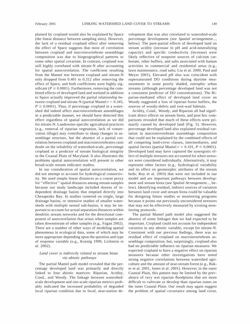
Land cover is indirectly related to stream biota viaabiotic pathways.—To relate land cover to stream biotavia abiotic pathways, we extended the partial Manteltest into a path-analytical framework (e.g., Leduc et al.1992, King et al. 2004). Spatial, land-cover, and abioticvariables are arranged in a hierarchical manner so thatvariation explained by confounding variables is fac-tored out, and the remaining variation in the responsevariable can be evaluated using the predictor variableof interest. This approach yields a pure-partial corre-lation—variation that cannot be explained by all of theother confounding variables in the analysis. To visu-alize the results, significant pure-partial correlations aresynthesized in a diagram that depicts pathways of sig-nificant relationships among variables (Fig. 5). Al-though this approach is conservative, a significantpure-partial relationship can afford compelling evi-dence for a potential causal pathway between land cov-er and biota (King et al. 2004).

We selected a suite of physical and chemical vari-ables measured by the MBSS as reach-scale abioticpredictors of macroinvertebrate assemblage composi-tion. We evaluated the simple relationship betweeneach variable and macroinvertebrate assemblage com-position using nonmetric multidimensional scaling(nMDS) ordination (Minchin 1987) and simple Manteltests. The ordination helped us visualize the directionand magnitude of abiotic correlations with composi-tion, whereas the Mantel tests helped confirm whichvariables were most strongly related to compositionusing the raw distance matrices. We selected variablesthat were most strongly correlated with macroinver-tebrate composition and removed redundant metrics ofa particular stream attribute (e.g., stream habitat) thatwere necessarily collinear, unless they appeared to ac-

count for a unique component of variation. This anal-ysis helped us identify the following groups of vari-ables to be used as individual distance matrices in thepartial Mantel path model: Watershed area (in hect-ares); Riparian (shading, remoteness, aesthetic rating,minimum width of riparian forest buffer); Gradient(slope, average velocity, velocity–depth diversity);Size (maximum depth, average width, average thalwegdepth); Woody (number of pieces of woody debris andnumber of root wads); SubQual. (in-stream habitat, epi-faunal substrate, pool quality, riffle quality, embed-dedness); NO3-N (nitrate-nitrogen), DOC (dissolvedorganic carbon); Cond. (specific conductivity); Acidity(pH and acid-neutralizing capacity); DO (dissolved ox-ygen); and Temp. (temperature) (see Appendix A).These groups of variables were converted into indi-vidual distance matrices using Euclidean distance. In-dividual variables in multi-variable distance matriceswere first standardized to z-scores (Legendre and Le-gendre 1998) so that each variable was weighted equal-ly in the matrix. Prior to standardization and conversionto distance matrices, some individual variables weretransformed to improve linearity and reduce heteros-cedasticity (arcsine square root for percentage vari-ables; log10 for continuous variables; see Appendix A).

We arranged distance matrices based on our inter-pretation of their hierarchical structure and causal or-der. This resulted in five levels of organization: spatial(Space, Watershed area); land cover (Developed, Wet-land, Cropland); indirect site-level abiotic variables(Riparian, Gradient, Size); direct site-level abiotic var-iables (Temp., DO, Acidity, Cond., DOC, NO3-N,SubQual., Woody); and the biological response vari-able (Macroinvertebrate assemblage composition). Weused this framework to specify appropriate covariatesfor each partial Mantel test. For all tests, we accountedfor Space and Watershed area, as these were spatialfactors that could confound apparent relationships atany level in the analysis. Furthermore, we accountedfor variation explained by other matrices in the samelevel of the hierarchy and examined the residual effectof each individual matrix on each matrix in the levelimmediately below it. These pathways representedpure-partial direct effects. However, we also tested forresidual effects between indirect predictors and mac-roinvertebrate composition by factoring out variationexplained by matrices on the same level and all levelsbelow them (e.g., a significant effect of developed landcover on macroinvertebrate composition after account-ing for abiotic intermediaries). Greater details on meth-ods and rationale for partial Mantel path models arepresented in King et al. (2004).

Spatial arrangement may be an important modulatorof watershed land-cover effects on stream ecosys-tems.—We explored the effect of within-watershed ar-rangement of land cover by relating macroinvertebrateassemblages to three ways of representing land cover:(1) percentage developed land in the watershed, (2)


TABLE 1. Pearson product-moment correlation matrix of watershed percentage land-coversummaries from the Coastal Plain physiographic province, Maryland, USA.

Land cover

Land cover

Developed Forested Cropland Wetland

Developed · · ·Forested 20.40**** · · ·Cropland 20.51**** 20.34**** · · ·Wetland 20.43**** 0.11NS 0.49**** · · ·

Note: Watersheds correspond to the 295 stream sites sampled by the Maryland BiologicalStream Survey (MBSS) in 1995–1997 (see Fig. 1).

**** P # 0.0001; NS, not significant (P . 0.05).

percentage developed land within a 250-m radius bufferaround the sampling station, and (3) percentage de-veloped land weighted by its inverse distance to thesampling station. We focused on developed land be-cause our other analyses showed that it was the primaryland-cover class linked to changes in macroinvertebrateassemblage composition (see Results, below). Prelim-inary analysis using station and stream buffers of var-ious sizes also indicated that macroinvertebrate com-position was more sensitive to development near thestation than along the entire stream corridor in the wa-tershed, so we retained the 250-m station buffer forfurther analysis. We used linear rather than flow-lengthdistance because we did not expect the effect of de-velopment to be transmitted solely by hydrologic pro-cesses (see Results, below).

As a response variable, we used axis scores that cor-responded most closely to increasing development inwatersheds from an nMDS ordination of genus-levelassemblage composition (BCD). The nMDS producedindividual site and taxa scores representing a univariateindex of taxonomic dissimilarity among sites—increas-ingly positive nMDS scores represented relatively di-verse macroinvertebrate assemblages composed ofmany pollution-sensitive taxa, while increasingly neg-ative scores corresponded to assemblages dominatedby taxa typically associated with impaired streams (Ap-pendix B). These nMDS scores could be evaluatedgraphically, which improved our ability to contrast sen-sitivity of responses among the three developed-landmetrics. Scatterplots of nMDS scores and developed-land metrics suggested a potential threshold response,so we evaluated the effect of spatial arrangement bycontrasting the amount of development that may haveresulted in a threshold, as quantified using nonpara-metric change-point analysis (nCPA; Qian et al. 2003,King and Richardson 2003). Change-point analysis es-timates the numerical value of a predictor, x, resultingin a threshold in the response variable, y, representedas the cumulative probability of a threshold. We hy-pothesized that if developed land near the samplingstation had a greater influence on stream biota, thenthreshold levels of percentage developed land wouldbe lower using the 250-m buffer and the IDW thanthreshold levels of unweighted developed land in the

watershed. Ordination and changepoint analyses wereconducted in PC-ORD 4.9 (MjM Software, GlenedenBeach, Oregon, USA) and in S-Plus 2000 using thecustom function nonpar.chngp (Qian et al. 2003), re-spectively.

After previous analyses (see Results, below) showedthat stream nitrate-N concentrations were stronglylinked to percentage cropland in watersheds, we ex-plored this relationship further by contrasting resultsfrom three watershed size classes determined by the33rd and 66th size percentiles in our data set. We thencompared these regressions on simple watershed per-centages with those using percentage cropland weight-ed by either the linear or flow-length inverse distanceto the sampling station or streams. Analyses reportedin Results are limited to linear station IDWs becauselinear and flow-length distance-to-station IDWs cap-tured virtually the same amount of variation in nitrate-N concentrations, but both of these IDWs capturedmore variation in nitrate-N than IDWs based on dis-tance to stream. Prior to analysis, we log10–transformednitrate-N concentrations and used partial correlationanalyses to remove variation attributable to percentagedeveloped land in watersheds.

RESULTS

Land-cover class percentages are not independent

A Pearson product-moment correlation matrix of thefour land-cover variables (N 5 295 stream sites sam-pled; Table 1) revealed a negative, triangular relation-ship among developed, cropland, and forested landcovers (i.e., all three dominant classes were negativelycorrelated with each other). Wetland cover tended topositively covary with cropland and negatively covarywith development. However, wetlands were only weak-ly correlated with forest cover despite sharing the for-ested wetland class.

Percentage cropland was highly positively correlatedwith nitrate-N (r 5 0.67, P # 0.0001; Fig. 3A) whileforest was negatively correlated with nitrate-N (r 520.57, P # 0.0001). Percentage wetland was positivelycorrelated to nitrate-N (r 5 0.21, P 5 0.0002), whereasincreasing percentage developed land appeared to re-duce nitrate-N (r 5 20.19, P 5 0.0011; Fig. 3). How-


FIG. 3. Simple correlation of (A) percentage cropland and(B) percentage developed land cover in watersheds withstream nitrate-N concentrations in Coastal Plain streams, and(C) the partial correlation between developed land cover andnitrate-N after the effect of cropland was removed.

ever, after the use of partial correlation analysis to fac-tor out the effect of cropland, correlations between bothpercentage developed land and percentage wetland andnitrate-N residuals were altered. The relatively highconcentrations of nitrate-N observed at low percent-ages of development (Fig. 3B) were markedly reducedwhen expressed as residuals after the effect of croplandhad been removed (Fig. 3C). Consequently, the direc-tion of the correlation reversed, yielding a significant,positive relationship (partial r 5 0.21, P 5 0.0003;Fig. 3C). Similarly, factoring out the effect of croplandidentified a weak but negative correlation between per-centage wetland and nitrate-N (partial r 5 20.15, P 50.021).

Land cover is spatially contagious and covarieswith the physical template

We estimated the degree of spatial contagion, or au-tocorrelation, in each land-cover class using the lineardistance between sampling sites, or Space, as a pre-dictor. Results from simple Mantel tests on land-coverpercentages indicated that they were spatially autocor-related among watersheds (Mantel r 5 0.07–0.48, P #0.0001). The spatial distributions of wetland and crop-land were particularly contagious, consistent with largeamounts of these land covers observed in the outerCoastal Plain (Fig. 1).

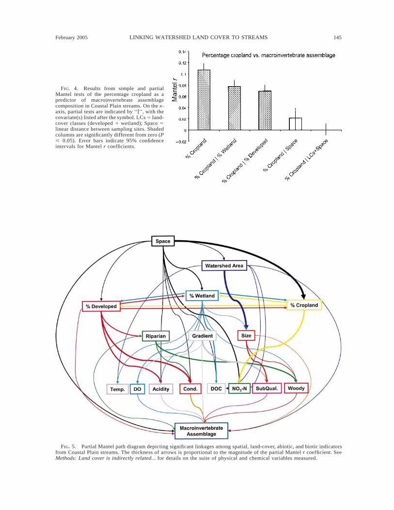
Percentage developed, percentage cropland, and per-centage wetland each were significant predictors ofmacroinvertebrate assemblage composition (simpleMantel test, Mantel r 5 0.193 (developed), 0.107 (crop-land), 0.114 (wetland); all P # 0.0001). All three land-cover classes remained significant predictors of com-position after the effect of each competing land coverwas removed; however, the magnitude of the correla-tions dropped for cropland (partial Mantel r 5 0.053,P 5 0.0002) and wetland (partial Mantel r 5 0.054, P# 0.0001). In contrast, percentage developed land re-mained a relatively strong correlate of composition af-ter removing the combined effects of percentage crop-land and percentage wetland (partial Mantel r 5 0.172,P # 0.0001). Factoring out the spatial component ofvariation in addition to the competing land-cover per-centages reduced the magnitude of the wetland effectto a level of marginal statistical significance (partialMantel r 5 0.039, P 5 0.013) and completely elimi-nated the correlation between cropland and composi-tion (partial Mantel r 5 0.002, P 5 0.902; Fig. 4). Infact, Space alone explained most of the variation incomposition that could be attributed to cropland (par-tial Mantel r 5 0.021, P 5 0.100; Fig. 4). Developedland was still a highly significant predictor of com-position after factoring out the effects of Space, crop-land, and wetland (partial Mantel r 5 0.173, P #0.0001).

Land cover is indirectly related to stream biotavia abiotic pathways

The pathways in Fig. 5 represent significant partialcorrelations between distance matrices, including path-


FIG. 4. Results from simple and partialMantel tests of the percentage cropland as apredictor of macroinvertebrate assemblagecomposition in Coastal Plain streams. On the x-axis, partial tests are indicated by ‘‘z’’, with thecovariate(s) listed after the symbol. LCs 5 land-cover classes (developed 1 wetland); Space 5linear distance between sampling sites. Shadedcolumns are significantly different from zero (P# 0.05). Error bars indicate 95% confidenceintervals for Mantel r coefficients.

FIG. 5. Partial Mantel path diagram depicting significant linkages among spatial, land-cover, abiotic, and biotic indicatorsfrom Coastal Plain streams. The thickness of arrows is proportional to the magnitude of the partial Mantel r coefficient. SeeMethods: Land cover is indirectly related... for details on the suite of physical and chemical variables measured.


FIG. 6. Scatterplots of the threshold effect of developedland on macroinvertebrate assemblage composition (Bray-Curtis dissimilarity expressed as nonmetric multidimensionalscaling [nMDS] Axis 1 scores). (A) Percentage developedland in the watershed. (B) Percentage developed land withina 250-m radius buffer of the sampling station. (C) Percentagedeveloped land in the watershed weighted by its inverse dis-tance (IDW; in meters) to the sampling station. The dottedlines indicate the cumulative probability of an ecologicalthreshold in response to increasing percentage developedland. Samples within the watershed-scale threshold zone of21–32% developed land in panel (A) are highlighted in blackin panels (A)–(C).

ways representing residual effects between matricesseparated by more than one hierarchical level. For brev-ity, here we describe only the significant pathways as-sociated with percentage developed land and percent-age cropland (see Fig. 5 for all significant partial Man-tel results).

Percentage developed land was directly and indi-rectly linked to several abiotic matrices. Developedland had direct linkages with Riparian (independent ofcompeting land-cover classes and spatial matrices; par-tial Mantel r 5 0.278, P # 0.0001) and Acidity andCond. (specific conductivity) (independent of inter-mediate effects of Riparian, Gradient, and Size, pluscompeting land-cover classes and spatial matrices, par-tial Mantel r 5 0.081 and 0.346, respectively; P #0.0001). Developed land also had indirect linkages withCond. (partially due to the direct effect of developmenton Riparian; partial Mantel r 5 0.167, P # 0.0001),and Woody (partially due to the direct effect of de-velopment on Riparian, partial Mantel r 5 0.263, P #0.0001). Percentage cropland, on the other hand, wasnot linked to any abiotic variable, with the exceptionof nitrate-N.

Acidity, Cond., Woody, and Riparian all had signif-icant direct effects on macroinvertebrate assemblages,and these effects were mostly attributable to percentagedeveloped land (Fig. 5). Percentage developed landalso explained variation in macroinvertebrate assem-blage composition that could not be explained by thecombined effect of all competing land-cover classes,abiotic intermediaries, and spatial factors (partial Man-tel r 5 0.101, P # 0.0001). There was no effect ofpercentage cropland on macroinvertebrate assemblagecomposition.

Spatial arrangement may be an important modulatorof watershed land-cover effects on stream ecosystems

Change-point analysis indicated that as little as 21%developed land in watersheds may result in a thresholdin the biotic composition of Coastal Plain streams (Fig.6A). Macroinvertebrate assemblage compositionchanged markedly between 21 and 32% developedland, and there was nearly a 100% probability thatsharp changes in taxonomic composition would occurbeyond 32% developed land. In contrast, there was a5% probability that as little as 1% developed land andnearly a 100% probability that .22% developed landin a 250-m buffer around each sampling station wouldalter stream macroinvertebrate assemblages (Fig. 6B).Here, many of the high-scoring samples that corre-sponded to watersheds with 21–32% development (theapparent watershed-scale threshold zone) actually hadrelatively little developed land in the 250-m buffer(Fig. 6B). However, many low-scoring samples withinthe watershed threshold zone also had little-to-no de-veloped land in the buffer. Contrasting watershed- andbuffer-scale results (Fig. 6A, B) with those obtainedusing inverse distance weighted (IDW) percentage de-

veloped land (Fig. 6C) suggested that development nearthe station had a greater effect on macroinvertebrateassemblages, but developed land elsewhere in the wa-tershed also influenced stream condition. The apparentthreshold zone using IDW percentage developed landwas 18–23%, much lower than the threshold zone cor-


FIG. 7. Regressions of stream nitrate-N concentrations on percentage cropland corrected for percentage developed landin the watershed in (A) large, (B) medium, and (C) small watersheds; and (D) percentage cropland in small watershedsweighted by its inverse distance (IDW) to station. Small watersheds with .25% cropland (unweighted) are indicated by solidsymbols. See Fig. 4 legend for explanation of partial-residuals labels.

responding to unweighted percentage developed landin the watershed. Moreover, high-scoring macroinver-tebrate samples within the watershed-scale thresholdzone (Fig. 6A) shifted to the left of the distance-weight-ed development threshold, but, contrary to the 250-mbuffer results (Fig. 6B), most of the low-scoring mac-roinvertebrate samples exceeded the threshold (Fig.6C).

Overall, percentage cropland was a strong predictorof stream nitrate-N in the Coastal Plain, and this re-lationship was slightly stronger after accounting forpercentage development (r 5 0.713, P , 0.0001, N 5295 sites). Regression slopes were similar among wa-tershed size classes (0.0092, 0.0124, and 0.0126 forsmall, medium, and large classes, respectively) but thevariance explained by these models varied markedly(Fig. 7). Large watersheds (.2600 ha) exhibited thestrongest correlation between percentage cropland andstream nitrate-N (Fig. 7A), but there was a trend towardweaker relationships in medium (600–2600 ha; Fig.7B) and small (,600 ha; Fig. 7C) watersheds.

Inverse-distance weighted percent cropland did notimprove predictions of nitrate-N over unweighted per-

centage cropland across all watersheds (r 5 0.702), inlarge (r 5 0.762), or in medium watersheds (r 5 0.626).Moreover, IDW percentage cropland yielded nearlyidentical slopes among all watershed size classes(0.0095, 0.0121, and 0.0129 for small, medium, andlarge, respectively). However, in small watersheds,IDW percentage cropland was a stronger predictor thanunweighted percentages and this effect was particularlyapparent in watersheds with $25% cropland (Fig. 7D).When watersheds with ,25% cropland (unweighted)were excluded from the analysis, partial correlationsbetween IDW percentage cropland and nitrate in-creased from 0.446 to 0.554 in small watersheds, butdecreased from 0.362 to 0.267 in large and 0.104 to0.043 in medium watersheds.

DISCUSSION

Land-cover class percentages are not independent

One of the most common uses of watershed land-cover data is to relate the percentages of specific land-cover classes (e.g., cropland) to stream indicator datausing simple linear correlation or regression analysis


(Van Sickle 2003). This is often conducted as an ex-ploratory series of correlations or stepwise multipleregressions in which several land-cover classes areused to predict a response variable. Land-cover vari-ables that yield the largest correlations are often in-ferred as related in some way, possibly causally, to theresponse variable. However, few investigators explic-itly acknowledge the fundamental limitation that land-cover percentages among watersheds tend to be highlycollinear (inter-correlated) so that a significant rela-tionship between a response variable and one land-cover variable may be accompanied by significant re-lationships with one or more other land-cover classes.It is very difficult to interpret results from such analyseswithout a clear understanding of the correlation struc-ture among land-cover variables and the ecological pro-cesses that yield that structure (MacNally 2000).

We used partial correlation analysis to factor out theeffect of cropland and test for independent correlationsbetween the remaining land-cover variables and thenitrate-N residuals. Here, the relatively high concen-trations of nitrate-N observed at low percentage de-veloped land were markedly reduced in the residualsafter factoring out the effect of cropland. Consequently,the direction of the correlation of nitrate-N and devel-oped land reversed, yielding a significant, positive re-lationship consistent with our expectations that devel-oped lands are nitrate-N sources (Jordan et al. 2003,Weller et al. 2003). By removing the overwhelmingeffect of cropland, we were able to isolate the inde-pendent effect of developed land. Similarly, factoringout the effect of cropland allowed us to identify a weakbut negative correlation between percentage wetlandand nitrate-N that matched our understanding of wet-lands as N sinks rather than sources (Weller et al. 1996,Baker et al. 2001). Thus, the effects of developed landand wetland on nitrate-N as inferred from simple cor-relations were very misleading. Only after consideringthe effect of other, collinear land-cover classes werewe able to isolate the individual effect of each class.

Although our initial explorations of the correlationbetween land-cover percentages and stream nitrate-Nwere ecologically misleading, they made sense statis-tically. The highest nitrate-N concentrations were ob-served in watersheds with a high percentage cropland,and high percentage cropland necessarily resulted in arelatively low percentage developed land. Therefore,developed land would logically be negatively corre-lated with nitrate-N using simple correlation analysis(Fig. 3B). The positive simple correlation of the per-centage wetland with nitrate-N was misleading for adifferent reason. Percentage cropland and percentagewetland were positively correlated because wetlandsspatially covaried with cropland on the outer CoastalPlain (Fig. 1, Table 1), so wetlands superficially ap-peared to increase nitrate-N concentrations relative toother land-cover classes.

Although these examples may seem somewhat ele-mentary, the analytical problems presented by collin-earity among land-cover classes are not trivial and canaffect virtually any broad-scale watershed study. Whereonly two predominant land-cover classes occur, itwould not make sense to factor out the effect of oneclass prior to examining the effect of the other becausetheir mutual effect would be captured when one land-cover type is used as a predictor. However, this scenariois an exception, and competing land-cover classes willneed to be accounted for in most studies.

Although we used partial-correlation analysis to il-lustrate the problem of land-cover collinearity, multi-ple-regression analysis also isolates the residual effectof each predictor in a similar way. However, our partial-correlation approach forced us to evaluate the inter-relationships of all pairs of land-cover predictors andtheir independent effects on nitrate rather than relyingon statistical software to identify the ‘‘best’’ suite ofpredictors, as is commonly done using stepwise mul-tiple regression. We contend that the latter approachmay sequentially identify the strongest predictors butobscure the fact that very similar results could havebeen obtained using collinear, competing land-coverclasses excluded by the stepwise selection process. Thegoal of our analysis was not to simply build the bestpredictive model, but to try to elucidate how differentland-cover classes may be linked to each other and tostream conditions. We suggest partial-correlation anal-ysis may further serve as a fundamental first step forbuilding such predictive models (e.g., Van Sickle 2003,Van Sickle et al. 2004).

Land cover is spatially contagious and covarieswith the physical template

We expected that macroinvertebrate assemblagecomposition would be affected by increasing percent-age cropland (e.g., Roth et al. 1996). Cropland was asignificant but not a strong correlate of macroinverte-brate composition when we used a simple Mantel test(Fig. 4). The relatively low influence of cropland fur-ther decreased when development and wetland effectswere removed, suggesting that much of the apparentcropland effect was indicating an absence of developedland and presence of wetland rather than the presenceof cropland. This interpretation was reinforced whenthe magnitude of the effect of developed land scarcelydecreased after accounting for cropland and wetland.Thus, the effects of cropland, wetland, and developedland were not ‘‘canceling’’ each other out in the partialMantel analysis. Instead, cropland simply did not ex-plain much unique variation in composition.

The effect of spatial autocorrelation on the relation-ships between cropland and macroinvertebrates wasmore interesting (Fig. 4). Given the high degree ofspatial contagion in the distribution of cropland in theCoastal Plain (simple Mantel r 5 0.481), we expectedthat some of the variation in macroinvertebrates ex-


plained by cropland would also be explained by Space(the linear distance between sampling sites). However,the lack of a residual cropland effect after removingthe effect of Space suggests that most of correlationbetween cropland and macroinvertebrate assemblagecomposition was due to biogeographical patterns orsome other spatial covariate. In contrast, cropland wasstill highly correlated with nitrate-N after accountingfor spatial autocorrelation. The coefficient resultingfrom the Mantel test between cropland and nitrate-Nonly dropped from 0.401 to 0.312 after removing theeffect of Space, and both coefficients were highly sig-nificant (P # 0.0001). Furthermore, removing the com-bined effects of developed land and wetland in additionto Space actually improved the partial relationship be-tween cropland and nitrate-N (partial Mantel r 5 0.345,P # 0.0001). Thus, if percentage cropland in a water-shed did indeed affect macroinvertebrate assemblagesin a predictable manner, we should have detected thiseffect regardless of spatial autocorrelation as we didfor nitrate-N. Landowner-specific agricultural practices(e.g., removal of riparian vegetation, lack of conser-vation tillage) may contribute to sharp changes in as-semblage structure, but the absence of a partial cor-relation between cropland and macroinvertebrates castsdoubt on the reliability of watershed-scale, percentagecropland as a predictor of stream biological integrityin the Coastal Plain of Maryland. It also illustrates theproblems spatial autocorrelation will present to otherbroad-scale stream indicator studies.

In our consideration of spatial autocorrelation, wedid not attempt to account for hydrological connectiv-ity. We used simple linear distances as a coarse proxyfor ‘‘effective’’ spatial distances among stream samplesbecause our study landscape included dozens of in-dependent drainage basins that emptied directly intoChesapeake Bay. In studies centered on single, largedrainage basins, or intensive studies of smaller water-sheds with multiple nested sub-basins, it may be im-portant to account for actual separation distances withindendritic stream networks and for the directional com-ponent of autocorrelation that arises when samples aretaken downstream of other samples (e.g., Fagan 2002).There are a number of other ways of modeling spatialphenomena in ecological data, some of which may bemore appropriate depending upon the question and typeof response variable (e.g., Koenig 1999, Lichstein etal. 2002).

Land cover is indirectly related to stream biotavia abiotic pathways

The partial Mantel path model revealed that the per-centage developed land was primarily and directlylinked to four abiotic matrices: Riparian, Acidity,Cond., and Woody. The linkage between watershed-scale development and site-scale riparian metrics prob-ably indicated the increased probability of degradedlocal riparian condition due to local, near-station de-

velopment that was also correlated to watershed-scalepercentage development (see Spatial arrangement...,below). The pure-partial effects of developed land onstream acidity (increase in pH and acid-neutralizingcapacity) and specific conductivity (increase) werelikely reflective of nonpoint sources of calcium car-bonate, other buffers, and salts associated with humanactivities in commercial and residential areas (e.g.,lawn maintenance, road salts; Liu et al. 2000, Paul andMeyer 2001). Elevated pH also was coincident withsupersaturated DO conditions during daytime mea-surements in some poorly shaded, eutrophic urbanstreams (although percentage developed land was nota consistent predictor of DO concentrations). The Ri-parian-mediated effect of developed land cover onWoody suggested a loss of riparian forest buffers, thesources of woody-debris and root-wad habitats.

Acidity, Cond., Woody, and Riparian all had signif-icant direct effects on stream biota, and post hoc com-parisons revealed that much of these effects were pri-marily caused by developed land (Fig. 5). However,percentage developed land also explained residual var-iation in macroinvertebrate assemblage compositionthat could not be explained by the combined effects ofall competing land-cover classes, intermediaries, andspatial factors (partial Mantel r 5 0.101, P # 0.0001).Developed land may have captured the synergistic ef-fect of multiple stressors not accounted for when stress-ors were considered individually. Alternatively, it mayrepresent other factors (e.g., hydrological variabilityand its effect on geomorphic attributes of the streambeds; Roy et al. 2003) that were not included in ourmodel and are important pathways between develop-ment and stream biota (see Spatial Arrangement..., be-low). Identifying residual, indirect sources of variationbetween land cover and stream biota could be valuablefor designing future studies or monitoring programsbecause it points out previously unconsidered stressorsthat may not be effectively measured by existing mon-itoring protocols.

The partial Mantel path model also suggested theabsence of some linkages that we had expected to beimportant. Cropland could not account for independentvariation in any abiotic variable, except for nitrate-N.Consistent with our previous findings, there was noresidual effect of cropland on macroinvertebrate as-semblage composition, but, surprisingly, cropland alsohad no predictable influence on riparian measures. Weexpected cropland to have a negative effect on riparianmeasures because other investigations have notedstrong negative correlations between watershed agri-culture and the amount of near-stream forest (e.g., Bak-er et al. 2001, Jones et al. 2001). However, in the outerCoastal Plain, this pattern may be limited by the prev-alence of very wet riparian floodplains that are moredifficult to cultivate or develop than riparian zones onthe inner Coastal Plain. Our result may again suggestthe problem of spatial covariance among land cover,


the physical template, and stream indicators (Richardset al. 1997).

In addition to the absence of a cropland effect, watertemperature was not a significant correlate of macro-invertebrates in the path model despite its recognizedimportance to stream biota (Hawkins et al. 1997). Tem-perature was only weakly correlated to macroinvere-brates in the simple Mantel tests, thus collinearity withother variables in the path model played only a minorrole in its insignificance. However, temperature wasonly measured on one date from each stream locationand, consequently, was influenced by temporal varia-tion among dates or times of sampling during the Mary-land Biological Stream Survey study (Klauda et al.1998). Thus, the estimate of temperature used in ouranalysis was not as robust as a long-term, integratedmeasure. This may partially explain why Riparian ex-plained residual variation in the macroinvertebrate dataafter all of the in-stream measures had been factoredout of the path model. Riparian measures may havebeen acting as indicators of a temperature effect notcaptured by the temperature variable.

Analyzing potential abiotic pathways between landcover and stream biota is clearly complex. All of thevariables used in this path model were significant cor-relates of macroinvertebrate assemblage compositionusing ordination and simple Mantel tests. However,many of these relationships could not be separated fromspatial artifacts or variation shared with other abioticfactors. Our exploratory approach is conservative likea single-edged sword: a significant pure-partial effectmakes a strong case for a particular linkage, but thelack of an effect does not necessarily mean a variableis unimportant. We argue that a conservative approachis needed to make strong inference using correlativeanalyses because observational studies are confoundedby the complexity of ecological data and associatedspatial dependencies (Legendre 1993, Lichstein et al.2002). Therefore, our analysis was a series of steps thatforced us to think about how to interpret correlativeresults in the context of several confounding analyticalhurdles. We have produced a body of evidence thatsuggests that development was an important source ofstressors to Coastal Plain stream ecosystems, while wa-tershed-scale cropland was not as clearly linked tooverall stream condition as we expected. However,cropland was clearly linked to elevated nitrate-N con-centrations, and excessive nutrient loading, particularlynitrate-N, is one of the most important stressors to beconsidered in restoring and managing the ChesapeakeBay ecosystem (Correll 1987, Boesch et al. 2001).

Spatial arrangement may be an important modulatorof watershed land-cover effects on stream ecosystems

We found that the threshold of macroinvertebrate-assemblage response was more sensitive to increasesin developed land if development was located closerto the sampling station (Fig. 6). When we related de-

veloped land near a station to the macroinvertebrateresponse, we observed a lower percentage developedland threshold than that estimated using developmentacross the entire watershed. This result, together withour path analysis results, suggest that development hasits greatest effect when close to the sampling station,where development contributes to riparian degradationand reduced woody-debris recruitment. To explore thisquestion more completely, we highlighted sites withwhole-watershed percentage developed land near thethreshold levels of effect on macroinvertebrates (Fig.6A) and tracked the effect of 250-m station buffers andIDWs on the apparent distribution of these sites relativeto the threshold. Sites with near-threshold land-coverpercentages are of particular interest because greaterdevelopment across the watershed always results indegradation and there is little evidence that less de-velopment predictably degrades streams. Therefore,near-threshold watersheds are where we expect land-cover arrangement to have the greatest influence onmacroinvertebrate assemblages. When we quantifieddeveloped land for a 250-m buffer (Fig. 6B), all of thehigh-scoring macroinvertebrate samples (Fig. 6A)moved to the left along the development axis (Fig. 6B).These high-scoring sites—characterized by pollution-sensitive macroinvertebrate taxa (Appendix B)—hadmoderate percentages of developed land in their wa-tersheds and little or none within 250 m of the samplingstation. Distance weighting also moved the high-qual-ity sites further to the left on the development axis(Fig. 6C), but not as much because distant develop-ment, excluded from the buffer summary, was incor-porated into the development effect. In addition, manylow-quality near-threshold sites apparently had sub-stantial percentages of development outside 250 m andthe buffer analysis failed to discriminate these fromhigh-quality sites. In contrast, distance weighting shift-ed the positions of these same sites to the right side ofthe threshold. Thus, distance weighting accounted forboth the whole-watershed and local-scale effects of de-veloped land.

The NLCD (National Land Cover Database) land-cover data used in our analysis did not include imper-vious surface as a land-cover class. Impervious surfaceis recognized as an important landscape indicator inwatershed studies (e.g., Arnold and Gibbons 1996,Wang et al. 2001). Percentage developed land is likelyto be highly correlated to percentage imperviousness,but it is not equivalent (1:1). Thus, the numerical de-veloped-land thresholds reported in this study shouldnot be interpreted as percentage impervious-surfacethresholds. However, the clear biotic thresholds ob-served in response to percentage developed land sug-gest that a similar analysis using percentage impervioussurface is warranted and could be very useful for land-use planning and ecological forecasting in this region(Nilsson et al. 2003, Van Sickle et al. 2004).


We also examined the influence of land-cover ar-rangement on predictions of stream nitrate-N concen-trations, yet these results depended on watershed size.In regressions using percentage cropland corrected forthe occurrence of developed land, we observed lowerexplanatory power in smaller watersheds (Fig. 7C)compared to medium (Fig. 7B) or large (Fig. 7A) wa-tersheds, though the slopes of the responses were sim-ilar. Strayer et al. (2003) observed a size effect in theability of land cover to predict various stream indica-tors, possibly because land-cover arrangement is moreimportant in small watersheds. Our findings appear tosupport their observations and hypothesis. Althoughdistance weights did not improve predictions of streamnitrate-N concentrations among large or medium wa-tersheds, they provided a 6% improvement in theamount of variance explained across all small water-sheds, and an 11% increase in small watersheds with.25% cropland (Fig. 7D). Incorporating land-cover ar-rangement in predictions of nitrate-N concentrations isconsistent with the idea that landscape sinks can reducenutrient discharges (Weller et al. 1998). However, ourresults do not prove conclusively that the spatial ar-rangement of cropland has a significant effect on ni-trate-N concentrations. The distance measures de-scribed here only account for surface distance, and oth-er transport pathways, or alternate forms of proximity,may be important, especially for nitrate-N (Jordan etal. 1997a, Baker et al. 2001).

Distance weighting can account for land-cover ar-rangement effects on stream conditions that are missedby land-cover percentages in whole watersheds orneighborhood buffers. Certainly proximal land coveris important, but reliance on buffers alone ignores thepotential for simultaneous and synergistic effects ofwatershed-scale land cover. Further, land-cover per-centages in buffers can be so highly correlated withwatershed-scale land cover that their unique effect ona response variable is often indistinguishable from wa-tershed-scale effects (Richards et al. 1997, Jones et al.2001). Arrangement effects may differ among phys-iographic regions, land-cover classes, response vari-ables, and the specific biophysical processes involved;so it may be prudent to consider different proximitymeasures (both dependent on and independent of land-cover percentage and watershed size) and differentweighting schemes for each combination of land-coverclass and stream indicator. The metrics described hereare useful exploratory analyses that complement cur-rent watershed-scale perspectives and warrant furtherinvestigation.

CONCLUSION

As the need for broad-scale assessment of aquaticconditions increases, we will likely see a greater reli-ance on land cover as an indicator of aquatic condition.We have highlighted several common problems that canarise in the use and relating of land-cover data to eco-

logical indicators in streams. Correctly interpretingland-cover effects in the context of proportional inter-dependence, spatial autocorrelation, collinearity withintermediaries, and spatial arrangement are nearly uni-versal challenges facing researchers and managers en-gaged in the conservation and management of aquaticresources. These challenges influenced our interpreta-tion of land-cover patterns and our ability to detectrelationships between human activities and stream con-dition. Simple correlations with land-cover percentagesmay lead to incorrect interpretations of the magnitudeand even the direction of an effect. Previous studies ofaquatic condition may well have suffered from theseinterpretive problems.

The methods we present are certainly not the onlysolutions available. However, the consideration of land-cover class interdependence, autocorrelation, linkageswith abiotic intermediaries, and spatial arrangementshould become standards in indicator analyses. Oth-erwise, we risk obscuring the relationships betweenland-cover patterns and condition of stream ecosys-tems.

ACKNOWLEDGMENTS

We thank our colleagues in the Atlantic Slope Consortium(ASC) for support of this research and the numerous indi-viduals at the Maryland Department of Natural Resourceswho contributed to the collection of the MBSS data set. Wealso thank Christer Nilsson and two anonymous reviewersfor improving an earlier draft of this paper. This research wasfunded by a grant to the ASC project from the U.S. Envi-ronmental Protection Agency’s Science to Achieve Results(STAR) Estuarine and Great Lakes (EaGLes) program, USE-PA Agreement number R-82868401. Although the researchdescribed in this article has been funded by the United StatesEnvironmental Protection Agency, it has not been subjectedto the Agency’s required peer and policy review and thereforedoes not necessarily reflect the views of the Agency and noofficial endorsement should be inferred.

LITERATURE CITED

Allan, J. D., and L. B. Johnson. 1997. Catchment-scale anal-ysis of aquatic ecosystems. Freshwater Biology 37:107–111.

Arnold, C. L., and C. J. Gibbons. 1996. Impervious surface:the emergence of a key urban environmental indicator.American Planning Association Journal 62:243–258.

Baker, M. E., M. J. Wiley, and P. W. Seelbach. 2001. GIS-based hydrologic modeling of riparian areas: implicationsfor stream water quality. Journal of the American WaterResources Association 37:1615–1628.

Barbour, M. T., J. Gerritsen, B. D. Snyder, and J. B. Stribling.1999. Rapid bioassessment protocols for use in streamsand wadeable rivers: periphyton, benthic macroinverte-brates, and fish. EPA 841-B-99-002. U. S. EnvironmentalProtection Agency, Office of Water, Washington, D.C.,USA.

Boesch, D. F., R. B. Brinsfield, and R. E. Magnien. 2001.Chesapeake Bay eutrophication: scientific understanding,ecosystem restoration, and challenges for agriculture. Jour-nal of Environmental Quality 30:303–320.

Bray, J. R., and J. T. Curtis. 1957. An ordination of the uplandforest communities of southern Wisconsin. EcologicalMonographs 27:325–349.

Comeleo, R. L., J. F. Paul, and P. V. August. 1996. Rela-tionships between watershed stressors and sediment con-


tamination in Chesapeake Bay estuaries. Landscape Ecol-ogy 11:307–319.

Correll, D. L. 1987. Nutrients in Chesapeake Bay. Pages 298–320 in L. W. Hall, H. M. Austin, and S. K. Majumdar,editors. Contaminant problems and management of livingChesapeake Bay resources. Pennsylvania Academy of Sci-ence, Easton, Pennsylvania, USA.

Dutilleul, P., D. Sockwell, D. Frigon, and P. Legendre. 2000.The Mantel-Pearson paradox: statistical considerations andecological implications. Journal of Agricultural, Biologi-cal, and Ecological Statistics 5:131–150.

EPA [United States Environmental Protection Agency].2000a. Multi-Resolution Land Characteristics Consortium(MRLC) database. ^http://www.epa.gov/mrlcpage&

EPA [United States Environmental Protection Agency].2000b. Stressor identification guidance document. EPA/822/B-00/025. U. S. Environmental Protection Agency Of-fice of Water, Washington, D.C., USA.

Fagan, W. F. 2002. Connectivity, fragmentation, and extinc-tion risk in dendritic metapopulations. Ecology 83:3243–3249.

Faith, D. P., P. R. Minchin, and L. Belbin. 1987. Composi-tional dissimilarity as a robust measure of ecological dis-tance. Vegetatio 69:57–68.

Griffith, J. A., E. A. Martinko, J. L. Whistler, and K. P. Price.2002. Preliminary comparison of landscape pattern–nor-malized difference vegetation index (NDVI) relationshipsto Central Plains stream conditions. Journal of Environ-mental Quality 31:846–859.

Harding, J. S., E. F. Benfield, P. V. Bolstad, G. S. Helfman,and E. B. D. Jones. 1998. Stream biodiversity: the ghostof land use past. Proceedings of the National Academy ofSciences (USA) 95:14843–14874.

Hawkins, C. P., J. N. Houge, L. M. Decker, and J. W. Fem-inella. 1997. Channel morphology, water temperature, andassemblage structure of stream insects. Journal of the NorthAmerican Benthological Society 16:728–749.

Herlihy, A. T., J. L. Stoddard, and C. B. Johnson. 1998. Therelationship between stream chemistry and watershed landcover data in the mid-Atlantic region, US. Water, Air, andSoil Pollution 105:377–386.

Hunsaker, C. T., and D. A. Levine. 1995. Hierarchical ap-proaches to the study of water quality in rivers. BioScience45:193–203.

Janicki, A., M. Morgan, and J. Lynch. 1995. An evaluationof stream chemistry and watershed characteristics in themid-Atlantic coastal plain. Report Number CBRM-AD-95-2. Chesapeake Bay Research and Monitoring Division,Maryland Department of Natural Resources, Annapolis,Maryland USA.

Jenson, S. K., and J. O. Domingue. 1988. Extracting topo-graphic structure from digital elevation data for geographicsystem analysis. Photogrammic Engineering and RemoteSensing 54:1593–1600.

Jones, K. B., A. C. Neale, M. S. Nash, R. D. Van Remortel,J. D. Wickham, K. H. Riiters, and R. V. O’Neill. 2001.Predicting nutrient discharges and sediment loadings tostreams from landscape metrics: a multiple watershed studyfrom the United States Mid-Atlantic Region. LandscapeEcology 16:301–312.

Jordan, T. E., D. L. Correll, and D. E. Weller. 1997a. Effectsof agriculture on discharges of nutrients from Coastal Plainwatersheds of Chesapeake Bay. Journal of EnvironmentalQuality 26:836–848.

Jordan, T. E., D. L. Correll, and D. E. Weller. 1997b. Relatingnutrient discharges from watersheds to land use and stream-flow variability. Water Resources Research 33:2579–2590.

Jordan, T. E., D. E. Weller, and D. L. Correll. 2003. Sourcesof nutrient inputs to the Patuxent River estuary. Estuaries26:226–243.

King, R. S., and C. J. Richardson. 2003. Integrating bioas-sessment and ecological risk assessment: an approach todeveloping numerical water-quality criteria. EnvironmentalManagement 31:795–809.

King, R. S., C. J. Richardson, D. L. Urban, and E. A. Ro-manowicz. 2004. Spatial dependency of vegetation–envi-ronmental linkages in an anthropogenically influenced wet-land ecosystem. Ecosystems 7:75–97.

Klauda, R., P. Kazyak, S. Stranko, M. Southerland, N. Roth,and J. Chaillou. 1998. The Maryland Biological StreamSurvey: a state agency program to assess the impact ofanthropogenic stresses on stream habitat and biota. Envi-ronmental Monitoring and Assessment 51:299–316.

Koenig, W. D. 1999. Spatial autocorrelation of ecologicalphenomena. Trends in Ecology and Evolution 14:22–26.

Lammert, M., and J. D. Allan. 1998. Assessing biotic integ-rity of streams: effects of scale in measuring the influenceof land use/cover and habitat structure on fish and mac-roinvertebrates. Environmental Management 23:257–270.

Leduc, A., P. Drapeau, Y. Bergeron, and P. Legendre. 1992.Study of spatial components of forest cover using partialMantel tests and path analysis. Journal of Vegetation Sci-ence 3:69–78.

Legendre, P. 1993. Spatial autocorrelation: trouble or a newparadigm? Ecology 74:1659–1673.

Legendre, P., and M. Anderson. 1999. Distance-based re-dundancy analysis: testing multispecies responses in mul-tifactorial experiments. Ecological Monographs 69:1–24.

Legendre, P., and M.-J. Fortin. 1989. Spatial pattern and eco-logical analysis. Vegetatio 80:107–138.

Legendre, P., and L. Legendre. 1998. Numerical ecology.Second edition. Elsevier, Amsterdam, The Netherlands.

Lichstein, J. W., T. R. Simons, S. A. Shriner, and K. E. Fra-nzreb. 2002. Spatial autocorrelation and autoregressivemodels in ecology. Ecological Monographs 72:445–463.

Liu, Z.-J., D. E. Weller, D. L. Correll, and T. E. Jordan. 2000.Effects of land cover and geology on stream chemistry inwatersheds of Chesapeake Bay. Journal of the AmericanWater Resources Association 36:1349–1366.

MacNally, R. 2000. Regression and model-building in con-servation biology, biogeography, and ecology: the distinc-tion between—and reconciliation of—‘‘predictive’’ and‘‘explanatory’’ models. Biodiversity and Conservation 9:655–671.

Manly, B. F. J. 1997. Randomization, bootstrap, and MonteCarlo methods in biology. Second edition. Chapman andHall, London, UK.

Mantel, N. 1967. The detection of disease clustering and ageneralized regression approach. Cancer Research 27:209–220.

Mercurio, G., J. C. Chaillou, and N. E. Roth. 1999. Guideto using 1995–1997 Maryland Biological Stream Surveydata. Report number EA-99-5; prepared by Versar (Colum-bia, Maryland, USA) for Maryland Department of NaturalResources (Annapolis, Maryland, USA). ^http://www.dnr.state.md.us/streams/mbss/mbss pubs.html&

Minchin, P. R. 1987. An evaluation of the relative robustnessof techniques for ecological ordination. Vegetatio 69:89–107.

Nilsson, C., J. E. Pizzuto, G. E. Moglen, M. A. Palmer, E.H. Stanley, N. E. Bockstael, and L. C. Thompson. 2003.Ecological forecasting and the urbanization of stream eco-systems: challenges for economists, hydrologists, geomor-phologists, and ecologists. Ecosystems 6:659–674.

Norton, S. B. 2000. Can biological assessments discriminateamong types of stress? A case study from the Eastern Corn-belt Plains Ecoregion. Environmental Toxicology andChemistry 19:1113–1119.

O’Callaghan, J. F., and D. M. Mark. 1984. The extraction ofdrainage networks from digital elevation data. ComputerVision, Graphics, and Image Processing 28:323–344.


Officer, C. B., R. B. Biggs, J. L. Taft, L. E. Cronin, M. A.Tyler, and W. R. Boynton. 1984. Chesapeake Bay anoxia:origin, development, and significance. Science 223:22–27.

Omernik, J. M., A. R. Abernathy, and L. M. Male. 1981.Stream nutrient levels and proximity of agricultural andforest land to streams: some relationships. Journal of Soiland Water Conservation 36:227–231.

O’Neill, R. V., C. T. Hunsaker, K. B. Jones, K. H. Riiters, J.D. Wickham, P. M. Schwartz, I. A. Goodman, B. L. Jack-son, and W. S. Baillargeon. 1997. Monitoring environ-mental quality at the landscape scale. BioScience 47:513–519.

Orth, R. J., and K. A. Moore. 1983. Chesapeake Bay: anunprecedented decline in submerged aquatic vegetation.Science 222:51–54.

Osborne, L. L., and M. J. Wiley. 1988. Empirical relation-ships between land use/cover and stream water quality inan agricultural watershed. Journal of Environmental Man-agement 26:9–27.

Paul, M. P., and J. L. Meyer. 2001. Streams in the urbanlandscape. Annual Review of Ecology and Systematics 32:333–365.

Peterjohn, W. T., and D. L. Correll. 1984. Nutrient dynamicsin an agricultural watershed: observations on the role of ariparian forest. Ecology 65:1466–1475.

Qian, S. S., R. S. King, and C. J. Richardson. 2003. Twostatistical methods for the detection of environmentalthresholds. Ecological Modelling 166:87–97.

Richards, C., R. J. Haro, L. B. Johnson, and G. E. Host. 1997.Catchment and reach scale properties as indicators of mac-roinvertebrate species traits. Freshwater Biology 37:219–230.

Roth, N. E., J. D. Allan, and D. L. Erickson. 1996. Landscapeinfluences on stream biotic integrity assessed at multiplespatial scales. Landscape Ecology 11:141–156.

Roy, A. H., A. D. Rosemond, M. J. Paul, D. S. Leigh, andJ. B. Wallace. 2003. Stream macroinvertebrate response tocatchment urbanisation (Georgia, USA). Freshwater Biol-ogy 48:329–346.

Schuft, M. J., T. J. Moser, P. J. Wigington, D. L. Stevens, L.S. McAllister, S. S. Chapman, and T. L. Ernst. 1999. De-velopment of landscape metrics for characterizing riparian-stream networks. Photogrammetric Engineering and Re-mote Sensing 65:1157–1167.

Smouse, P. E., J. C. Long, and R. R. Sokal. 1986. Multipleregression and correlation extensions of the Mantel test ofmatrix correspondence. Systematic Zoology 35:627–632.

Sokal, R. R., and F. J. Rohlf. 1995. Biometry. Third edition.W. H. Freeman and Company, New York, New York, USA.

Soranno, P. A., S. L. Hubler, and S. R. Carpenter. 1996. Phos-phorous loads to surface waters: a simple model to account

for spatial pattern of land use. Ecological Applications 6:865–878.

Sponseller, R. A., E. F. Benfield, and H. M. Valett. 2001.Relationships between land use, spatial scale, and streammacroinvertebrate communities. Freshwater Biology 46:1409–1424.

Strayer, D. L., R. E. Beighley, L. C. Thompson, S. Brooks,C. Nilsson, G. Pinay, and R. J. Naiman. 2003. Effects ofland cover on stream ecosystems: roles of empirical modelsand scaling issues. Ecosystems 6:407–423.

Stribling, J. B., B. K. Jessup, J. S. White, D. Boward, andM. Hurd. 1998. Development of a benthic index of bioticintegrity for Maryland streams. Report Number CBWP-EA-98-3. Maryland Department of Natural Resources,Monitoring and Nontidal Assessment Division, Annapolis,Maryland, USA.

Turner, M. G., R. V. O’Neill, R. H. Gardner, and B. T. Milne.1989. Effects of changing spatial scale on landscape pat-tern. Landscape Ecology 3:153–162.

Urban, D., S. Goslee, K. Pierce, and T. Lookingbill. 2002.Extending community ecology to landscapes. Ecoscience12:200–212.

Van Sickle, J. 2003. Analyzing correlations between streamand watershed attributes. Journal of the American WaterResources Association 39:717–726.

Van Sickle, J., J. Baker, A. Herlihy, P. Bayley, S. Gregory,P. Haggerty, L. Ashkenas, and J. Li. 2004. Projecting thebiological condition of streams under alternative scenariosof human land use. Ecological Applications 14:368–380.

Wang, L., J. Lyons, P. Kanehl, and R. Bannerman. 2001.Impacts of urbanization on stream habitat and fish acrossmultiple spatial scales. Environmental Management 28:255–266.

Weigel, B. M. 2003. Development of stream macroinverte-brate models that predict watershed and local stressors inWisconsin. Journal of the North American BenthologicalSociety 22:123–142.

Weller, C. M., M. C. Watzin, and D. Wang. 1996. Role ofwetlands in reducing phosphorus loading to surface waterin eight watersheds in the Lake Champlain Basin. Envi-ronmental Management 20:731–730.

Weller, D. E., T. E. Jordan, and D. L. Correll. 1998. Heuristicmodels for material discharge from landscapes with ripar-ian buffers. Ecological Applications 8:1156–1169.

Weller, D. E., T. J. Jordan, D. L. Correll, and Z.-J. Liu. 2003.Effects of land use change on nutrient discharges from thePatuxent River watershed. Estuaries 26:244–266.

Yuan, L. L., and S. B. Norton. 2003. Comparing responsesof macroinvertebrate metrics to increasing stress. Journalof the North American Benthological Society 22:308–322.

APPENDIX A

A table summarizing the spatial, land cover, and environmental variables obtained from the NLCD and MBSS data sets(N 5 295 stream sites sampled), including distance-matrix assignments and data transformations, is available in ESA’sElectronic Data Archive: Ecological Archives A015-004-A1.

APPENDIX B

A table summarizing scientific names, nMDS Axis 1 scores, frequencies of occurrence, and tolerance values for allmacroinveretebrate taxa with at least 10 occurrences in the MBSS data set (N 5 295 stream sites sampled) is available inESA’s Electronic Data Archive: Ecological Archives A015-004-A2.

spatial considerations for linking … ecological applications, 15(1), 2005, pp. 137–153 q 2005 by...

Documents