1

Spatial and temporal dimensions to the taxonomic diversity of arthropods in an arid grassland savannah Fredrik Daleruma,b,c,*, J. Low de Vriesd, Christian W.W. Pirkd and Elissa Z. Cameronb,e a Research Unit of Biodiversity (UO, CSIC, PA), University of Oviedo, Mieres Campus, 33600 Mieres, Spain b Mammal Research Institute, Department of Zoology and Entomology, University of Pretoria, Private Bag X20, 0028 Pretoria, South Africa c Department of Zoology, Stockholm University, 106 91, Stockholm, Sweden d Department of Zoology and Entomology, University of Pretoria, Private Bag X20, 0028 Pretoria, South Africa e School of Zoology, University of Tasmania, Private Bag 50, Bobart, TAS 7001, Australia * Corresponding author E-mail: dalerumjohan@uniovi.es Journal of Arid Environment, 144, 21-30

2

ABSTRACT Quantifying the drivers of biodiversity variation is a key topic in contemporary ecology. While the geographic distribution of biodiversity is broadly determined by water and energy, local environmental conditions may be important. We valuated the relative effects of spatial and temporal variation on taxonomic diversity of ground living arthropod communities in central South Africa. Seasonal climate variation was a major driver of arthropod abundance, but seasonal effects differed between habitats. We did not find any evidence for modular community structures, even across different habitats, or any evidence for a nested pattern across seasons. Instead, we observed a spatial nestedness which was only partly related to specific habitats. Our results suggest that neutral processes had influenced arthropod community structure, but also that very local processes may have been pivotal in determining local and regional arthropod diversity. Such processes may not necessarily have been neutral, but could have been caused by niche deterministic processes acting at scales smaller the distinct habitat classes we used for our study. We further suggest that alterations in climate likely will have substantial effects on the spatial and temporal distribution of arthropod diversity in this arid region. Keywords alpha diversity, beta diversity, community, invertebrate, modularity, nestedness

3

1. Introduction Understanding drivers for the distribution of biological diversity across spatial and temporal scales has emerged as key a topic in contemporary ecology (Reiss et al. 2009). This interest has at least partly been fuelled by a realization of the critical roles biodiversity has for the functioning of ecosystems (Hooper et al. 2005), and subsequently also for the sustenance of humanity (Cardinale et al. 2012). The geographic distributions of biological organisms are broadly determined by interactions of available water and energy (Hawkins et al. 2003). These factors have generated a large scale latitudinal diversity gradient in which the equatorial zones generally contain more diverse biological communities than temperate or polar ones (Hillebrand 2004). However, although this latitudinal diversity gradient sets the ecological boundary conditions for patterns of biodiversity (Hubbel 2001), both local conditions as well as neutral processes such as genetic drift and random dispersal events may impose strong effects on the composition and structure of ecological communities (Rosensweig 1995, Alonso 2006). Such effects can not be ignored if we aim to fully understand how ecological communities have formed and are maintained.

Taxonomic diversity, which can be regarded as a discrete classification of phylogenetic relationships, may relate to both functional and phylogenetic aspects of diversity and can be seen as a proxy for these more specific diversity dimensions (Hooper et al. 2002). Taxonomic diversity is often partitioned into and components to distinguish between different scale-dependent characteristics of variation (Whittaker 1960). Alpha diversity quantifies the local diversity within a specific site, diversity quantifies the variability among sampling units for a given area at a given spatial scale, whereas diversity quantifies the total diversity of a group of locations and therefore represents regional diversity.

However, although diversity metrics are useful for assessing the amount of variation within and among biological communities, they do not fully describe patterns of species distributions across time and space (but see Anderson et al. 2011). In particular, both nested and modular patterns of the spatial distributions of species may be highly relevant for ecosystem properties, but are not readily quantified by various diversity metrics. Nested patterns of species distributions have been recognized since the early half of the past century (Hultèn 1938). Spatial nestedness indicates a distribution pattern where the distributions of the most widespread species also encompass the distribution of more localized ones (Galeano et al. 2009). Hence, with a truly nested spatial pattern all of the species present within species-poor locations are present within species-rich locations. The species rich locations therefore contain unique species and as a consequence species-poor locations do not contribute to the overall species richness of an area (Slipinski et al. 2012). Modularity describes the extent to which species are clustered into ‘modules’, where species are more ecologically associated within modules than they are across modules (Olesen et al. 2007). Modular patterns remain poorly incorporated into spatial ecology (Thèbault 2013). This is somewhat surprising, since the extent of modularity is expected to be an important property of ecological communities (Olesen et al. 2007).

Despite ample attention to spatial partitioning of diversity (e.g., Lande 1996, Crist et al. 2003, Gering et al. 2003, Ulrich et al. 2009), limited attention has been given to the temporal partitioning of species communities (Tylianakis et al. 2005). This is unfortunate, since temporal variation may have significant impact on both regional diversity as well as spatial variation of diversity among different habitats (Tylianakis et al. 2005, Rollin et al. 2015). Repeated studies on tropical invertebrate assemblages have suggested that temporal variation in species turnover may account for up to 20-25% of overall diversity within regions, which are values that are very close the variation attributed to spatial variation related to different habitats (DeVries et al. 1997, Tylianakis et al. 2005, see also Rollin et al. 2015). The temporal scale of sampling may also introduce substantial methodological bias in quantification of both species richness and diversity measures even in non-seasonal environments (Summerville and Crist 2005), and seasonal variation in climate may have profound variation on ecological communities as well (Wolda 1988).

4

Arthropoda is one the most diverse animal phylums with an estimated species richness of between 5 and 10 million extant species (Ødegaard 2000). Arthropod communities are important ecological components and have direct consequences on plant communities both through top-down processes and as a food source for organisms at higher trophic levels (Walker and Jones 2001). Since arthropods are both abundant and relatively easy to sample, they are frequently used as model organisms for studies evaluating how local environmental factors influence diversity (McGeoch 1998). However, rigid species-level evaluations of hyper-diverse taxa such as arthropods are logicistically daunting and may be subject to taxonomic uncertainty (Williams and Gaston 1994, Lawton et al. 1998, Cagnolo et al. 2002, Báldi 2003). Although the diversity and richness of higher taxon levels may be poor indicators of the diversity of other organism groups (Báldi 2003), they seem to correlate well with the diversity of finer taxonomic resolutions within these coarser groupings (Williams and Gaston 1994, Vanderklift et al. 1998, Báldi 2003, Bang and Faeth 2011). These observations are supported by theoretical arguments for diversity patterns to be robust against taxonomic scale (Storch and Sizling 2008).

Although climate may impose the ultimate boundary conditions for species ranges (Hawkins et al. 2003), the characteristics of local plant communities directly influence the abundance and composition of arthropod communities by acting both as a food source and as refugia (Southwood et al. 1979). Although stochastic processes may be important for local community assembly (Chase and Mayers 2011), there is generally a positive association between plant and arthropod diversity which may suggest that niche related processes are important for the composition of local arthropod assemblages. These patterns may be related to the ability of richer plant communities to host richer communities of herbivorous arthropods (Siemann et al. 1998), but also because of a positive secondary effect on predatory and parasitic arthropods (Southwood et al. 1979, Siemann et al. 1998). Furthermore, within the effects imposed by local vegetation characteristics, temporal variation in local climate may also influence the abundance and composition of arthropods at any given time (Wolda 1988).

Here we use data from a survey of ground living arthropods in central South Africa to evaluate how spatial variation within and across four distinct habitats and temporal variation primarily related to climate influenced abundance as well as and diversity of local arthropod communities. Because most arthropods have relatively limited dispersal abilities, we expect that broad scale environmental variables, including climate, have dictated the regional taxonomic pool of arthropods, but that local variation primarily in plant communities has defined the spatial variation in arthropod communities within this regional pool. Furthermore, we expect that temporal variation in climate has defined the community of arthropods within a specific site at any given time. We specifically evaluated the following predictions: (i) there will be an increase in abundance for all taxonomic groups during the wet compared o the dry season, (ii) there will be an increase in both alpha and beta diversity with increasing spatial scale, (iii) there will be will an increase in both alpha and beta diversity with increasing temporal scale, (iv) there will be a modular spatial pattern of arthopods among different habitats, and (v) there will be a nested temporal pattern of community composition within these modules, caused by seasonal variation in climate. We conducted the analyses at the taxonomic resolution of order, except for members of myriapods and arachnids, which were grouped across higher taxonomic ranks.

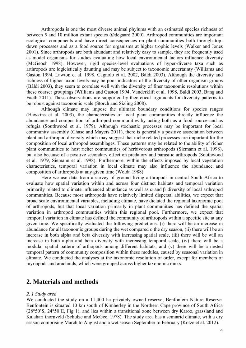
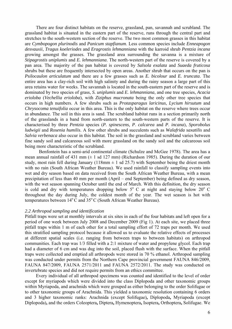
2. Materials and methods 2. 1 Study area We conducted the study on a 11,400 ha privately owned reserve, Benfontein Nature Reserve. Benfontein is situated 10 km south of Kimberley in the Northern Cape province of South Africa (28°50’S, 24°50’E, Fig 1), and lies within a transitional zone between dry Karoo, grassland and Kalahari thornveld (Schulze and McGee, 1978). The study area has a semiarid climate, with a dry season comprising March to August and a wet season September to February (Kotze et al. 2012).

5

Fig. 1. The location of Benfontein Game Reserve as well as the distribution of locations of pitfall trap sites within reserve.

6

There are four distinct habitats on the reserve, grassland, pan, savannah and scrubland. The grassland habitat is situated in the eastern part of the reserve, runs through the central part and stretches to the south-western section of the reserve. The two most common grasses in this habitat are Cymbopogon plurinodis and Panicum stapfianum. Less common species include Enneapogon desvauxii, Tragus koeleriodes and Eragrostis lehmanniana with the karroid shrub Pentzia incana growing amongst the grasses. The grassland area surrounding the savanna is a mixture of Stipagrostis uniplumis and E. lehmanniana. The north-western part of the reserve is covered by a pan area. The majority of the pan habitat is covered by Salsola exalata and Suaeda fruticosa shrubs but these are frequently intersected by open areas. Another shrub that occurs on the pan is Psilocaulon articulatum and there are a few grasses such as E. bicolour and E. truncata. The entire area has a clay-rich soil with high salinity and during the rainy season a large part of this area retains water for weeks. The savannah is located in the south-eastern part of the reserve and is dominated by two species of grass, S. uniplumis and E. lehmanniana, and one tree species, Acacia erioloba (Vechellia erioloba), with Ziziphus mucronata being the only other tree species that occurs in high numbers. A few shrubs such as Protasparagus laricinus, Lycium hirsutum and Chrysocoma tenuifolia occur in this area. This is the only habitat on the reserve where trees occur in abundance. The soil in this area is sand. The scrubland habitat runs in a section primarily north of the grasslands in a band from north-eastern to the south-western parts of the reserve. It is characterised by three Pentzia species (P. spinescens, P. calcarea and P. incana), Sporobolus ludwigii and Rosenia humilis. A few other shrubs and succulents such as Walafrida saxatilis and Salvia verbenaca also occur in this habitat. The soil in the grassland and scrubland varies between fine sandy soil and calcareous soil with more grassland on the sandy soil and the calcareous soil being more characteristic of the scrubland.

Benfontein has a semi-arid continental climate (Schulze and McGee 1978). The area has a mean annual rainfall of 431 mm (± 1 sd 127 mm) (Richardson 1985). During the duration of our study, most rain fell during January (118mm ± 1 sd 25.7) with September being the driest month with no rain (South African Weather Bureau). We used rainfall to classify sampling events into wet and dry season based on data received from the South African Weather Bureau, with a mean precipitation of less than 40 mm per month (April – end September) being defined as dry season, with the wet season spanning October until the end of March. With this definition, the dry season is cold and dry with temperatures dropping below 5o C at night and staying below 20o C throughout the day during July, the coldest month of the year. The wet season is hot with temperatures between 14o C and 35o C (South African Weather Bureau).

2.2 Arthropod sampling and identification Pitfall traps were set at monthly intervals at six sites in each of the four habitats and left open for a period of one week between July 2008 and December 2009 (Fig 1). At each site, we placed three pitfall traps within 1 m of each other for a total sampling effort of 72 traps per month. We used this stratified sampling protocol because it allowed us to evaluate the relative effects of processes at different spatial scales (i.e. ranging from between traps to between habitats) on arthropod communities. Each trap was 1/3 filled with a 2:1 mixture of water and propylene glycol. Each trap had a diameter of 6 cm and was dug into the soil, placed flush with the surface. When the pitfall traps were collected and emptied all arthropods were stored in 70 % ethanol. Arthropod sampling was conducted under permits from the Northern Cape provincial government FAUNA 846/2009, FAUNA 847/2009, FAUNA 2571/2011 and FAUNA 2572/2011. The study was conducted on invertebrate species and did not require permits from an ethics committee.

Every individual of all arthropod specimens was counted and identified to the level of order except for myriapods which were divided into the class Diplopoda and other taxonomic groups within Myriapoda, and arachnids which were grouped as either belonging to the order Solifugae or to other taxonomic groups of Arachnida. This yielded a taxonomic resolution containing 6 orders and 3 higher taxonomic ranks: Arachnida (except Solifugae), Diplopoda, Myriapoda (except Diplopoda), and the orders Coleoptera, Diptera, Hymenoptera, Isoptera, Orthoptera, Solifugae. We

7

opted for this broad classification for two primary reasons. First, a higher taxonomic resolution would have been largely impractical, and would have necessitated sub-sampling of data. We regarded that a complete data set, albeit with a coarser taxonomic resolution, would be informative than sub-sampled data at finer taxonomic resolution. Second, many arthropod groups of finer taxonomic ranks are poorly defined (e.g., Ødegaard 2000), and we also had few individuals of many finer scale groups. Our taxonomic resolution hence provided taxonomically robust data that enabled inclusion of all trapped arthropods without considering taxonomic groups with a very small number of trapped individuals. Since sparse matrices may provide poor quantifications of diversity and ecological interactions (Galeano et al. 2009, Heino et al. 2015), we regard this as an additional benefit of our classification. Although empirical data suggests some variation in terms of how well coarse scale taxonomic groupings represent finer ones (Bevilacqua et al. 2012, van Rijn et al. 2015), any taxonomic resolution that holds sufficient information to address the questions of concerns may be regarded as appropriate targets for analyses (Ellis 1985). Since diversity patterns are expected to be invariant of taxonomic resolution (Storch and Sizling 2008), we regard our data to be informative regarding the environmental influences on arthropod communities, albeit with the caveat of lacking some statistical power that may accompany biodiversity data at more refined taxonomic scales.

2.3 Data analyses Because of the large dominance of ants (Hymenoptera, family Formicidae) in the sample, we did separate analyses of the effects of season and habitat on abundance with ants included and excluded from the data. We conducted all analyses on diversity and taxonomic composition on data where all ants were excluded.

We used generalized linear mixed models with a Poisson error distribution and a log link to evaluate the effects of habitat and seasons on overall arthropod abundance. For the models, we used the raw count of arthropods collected in each single trap during each trapping session as response variable. We used habitat (as a four level factor including grass, pan, savannah, and shrub), season (as a two level factor including dry and wet seasons) and the two-way interaction as fixed effects. We fitted the models using trap nested within trap site which was nested within habitat as a nested factorial random effect structure, to account for spatial interdependence. To evaluate the relative effects of seasons within each habitat and of habitat within each season we fitted subset models within each habitat and each season. Pair-wise seasonal differences were evaluated from the subset models using Tukey contrasts (Hothorn et al. 2008).

We used the exponent of the Shannon-Wiener index (Shannon 1948) as a measure of diversity, which represents the hypothetical number of equally common taxonomic groups in a sample (i.e. effective number of taxonomic groups, Jost 2006). We quantified diversity across four spatial and three temporal scales. On a temporal scale we either quantified diversity separately for each monthly sample, as all samples pooled within a season, or as all samples pooled across the whole study period. For each of these temporal scales, we estimated diversity either for each trap separately, for pooled data from all traps within a sampling site, for pooled data from all traps within a habitat, and for pooled data from all traps within the study area. To evaluate the effect of temporal and spatial scales on diversity within and across habitats and seasons we used a permutation based linear model approach implemented in the R package lmPerm (Wheeler 2010), due to the inherent non-independence of data points across the different spatial and temporal scales. Furthermore, because the full sample design contained structural zeros (e.g., each month can only be attributed to one season, and hence not contribute to pooled samples across seasons), we created three subset models to evaluate specific hypotheses (Hector et al. 2010). In the first subset model, we excluded all data pooled across both seasons and across all habitats. In this model we used the estimated effective number of taxonomic groups as dependent variable, and season, habitat, spatial resolution (as a three level factor including trap, site, or all traps with each habitat), temporal resolution (as a two level factor including month and all trap occasions within a season) and all interactions as predictors. In the second subset model, we did

8

not include a monthly temporal resolution, and not samples pooled across all habitats. In this model, we used season (estimated as a three level factor including dry and wet seasons and both seasons combined), habitat (estimated as a four level factor including grass, pan, savannah, and shrub), spatial resolution (as a three level factor including trap, site, or all traps with each habitat) and all interactions. In the third subset model, we only included data pooled across all traps within each habitat or the whole study area. In this model, we used season (estimated as a three level factor including dry and wet seasons and both seasons combined), habitat (estimated as a five level factor including grass, pan, savannah, shrub, and all habitats combined), temporal resolution (as a two level factor including month and all trap occasions within or across seasons) and two-way interaction effects.

We quantified diversity as the Euclidean distances between each trap to relevant group centroids in a multidimensional space which dimensions were defined by the detected taxonomic groups (Anderson et al. 2006). To evaluate the effect of spatial scale on diversity within and between habitats, we calculated Euclidean distances to centroids for each trap site, each habitat and for the whole reserve. However, to enable a quantification of how much this spatial heterogeneity was influenced by variation in arthropod communities over time, we replicated each spatial centroid three times. First we calculated each of the three spatial centroids only on samples collected the same month, secondly on all samples collected the same season, and finally on samples pooled across all sample occasions. We also included a fourth category of centroid which had no spatial dimension. These were calculated on samples from each trap pooled across each season and both season combined. The distances to this centroid hence indicate the variation attributable only to temporal variation within and across seasons. We calculated the Euclidean distances on raw counts of individual arthropods from each taxonomic group for each trap. We used mixed linear models to evaluate the effect of space and time on variation in arthropod communities. Due to structural zeros, similarly to our analyses of diversity we created three subsets models. All models used the Euclidean distance as response variable and were fitted with trap nested within trap site nested within habitat as random effect structure. To evaluate interactions between habitat, season and the spatial and temporal resolution, we created two subset models, one excluding distances to centroids without a spatial dimension (i.e. centroids were calculated from samples aggregated across time from the same trap) and one excluding distances to centroids without any temporal variation (i.e. were centroids were calculated from samples aggregated across different locations but only from the same trapping occasion). In both models, we also excluded distances to centroids calculated across all samples pooled, since they reflect the overall diversity within the whole study area. These models included season, habitat, temporal resolution, spatial resolution and all interactions as categorical predictors. To enable evaluations of the full set of factor levels, we also created a model containing only the main effects of habitat, season, spatial resolution and temporal resolution. This model was fitted on all levels of spatial and temporal resolution.

We adopted methods from recent advances in the analyses of ecological networks (Miranda et al. 2014) to quantify the relative variation in arthropod community composition across spatial and temporal scales (e.g., Borthagaray et al. 2014). For these analyses, we created a matrix with the taxonomic groups as rows and the spatial sampling sites broken down into the two seasons as columns (Ulrich et al. 2009). Each cell represented the total number of arthropods of a specific taxonomic group trapped at each site for a given season, and hence allowed weighted quantifications of spatiotemporal patterns in community structure. We pooled samples across traps within sites and over all months within seasons to avoid excessive number of zero values in the interaction matrices. With this pooling, we also avoided potential confounding effects related to the non-independence of data from traps within each site.

We tested if there was evidence for spatial or temporal modularity in arthropod communities using the QuaBiMO algorithm (Dormann and Strauss 2014). This algorithm computes a modularity index (Q) that ranges from 0, which indicates that a community has no more links within modules than what is expected by chance, to a maximum value of 1, which

9

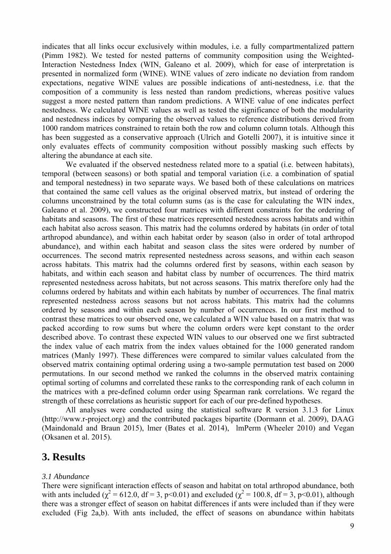
indicates that all links occur exclusively within modules, i.e. a fully compartmentalized pattern (Pimm 1982). We tested for nested patterns of community composition using the Weighted-Interaction Nestedness Index (WIN, Galeano et al. 2009), which for ease of interpretation is presented in normalized form (WINE). WINE values of zero indicate no deviation from random expectations, negative WINE values are possible indications of anti-nestedness, i.e. that the composition of a community is less nested than random predictions, whereas positive values suggest a more nested pattern than random predictions. A WINE value of one indicates perfect nestedness. We calculated WINE values as well as tested the significance of both the modularity and nestedness indices by comparing the observed values to reference distributions derived from 1000 random matrices constrained to retain both the row and column column totals. Although this has been suggested as a conservative approach (Ulrich and Gotelli 2007), it is intuitive since it only evaluates effects of community composition without possibly masking such effects by altering the abundance at each site.

We evaluated if the observed nestedness related more to a spatial (i.e. between habitats), temporal (between seasons) or both spatial and temporal variation (i.e. a combination of spatial and temporal nestedness) in two separate ways. We based both of these calculations on matrices that contained the same cell values as the original observed matrix, but instead of ordering the columns unconstrained by the total column sums (as is the case for calculating the WIN index, Galeano et al. 2009), we constructed four matrices with different constraints for the ordering of habitats and seasons. The first of these matrices represented nestedness across habitats and within each habitat also across season. This matrix had the columns ordered by habitats (in order of total arthropod abundance), and within each habitat order by season (also in order of total arthropod abundance), and within each habitat and season class the sites were ordered by number of occurrences. The second matrix represented nestedness across seasons, and within each season across habitats. This matrix had the columns ordered first by seasons, within each season by habitats, and within each season and habitat class by number of occurrences. The third matrix represented nestedness across habitats, but not across seasons. This matrix therefore only had the columns ordered by habitats and within each habitats by number of occurrences. The final matrix represented nestedness across seasons but not across habitats. This matrix had the columns ordered by seasons and within each season by number of occurrences. In our first method to contrast these matrices to our observed one, we calculated a WIN value based on a matrix that was packed according to row sums but where the column orders were kept constant to the order described above. To contrast these expected WIN values to our observed one we first subtracted the index value of each matrix from the index values obtained for the 1000 generated random matrices (Manly 1997). These differences were compared to similar values calculated from the observed matrix containing optimal ordering using a two-sample permutation test based on 2000 permutations. In our second method we ranked the columns in the observed matrix containing optimal sorting of columns and correlated these ranks to the corresponding rank of each column in the matrices with a pre-defined column order using Spearman rank correlations. We regard the strength of these correlations as heuristic support for each of our pre-defined hypotheses.

All analyses were conducted using the statistical software R version 3.1.3 for Linux (http://www.r-project.org) and the contributed packages bipartite (Dormann et al. 2009), DAAG (Maindonald and Braun 2015), lmer (Bates et al. 2014), lmPerm (Wheeler 2010) and Vegan (Oksanen et al. 2015).

3. Results

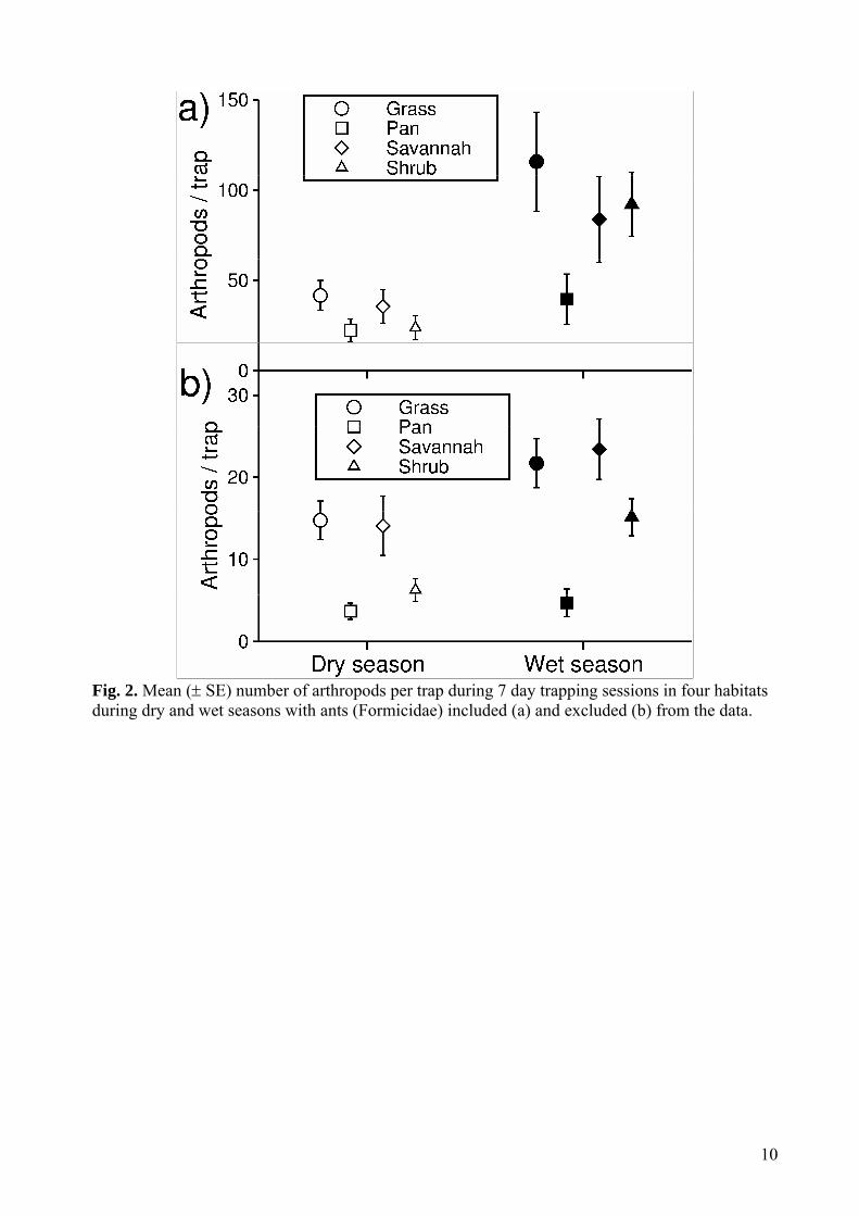
3.1 Abundance There were significant interaction effects of season and habitat on total arthropod abundance, both with ants included (χ2 = 612.0, df = 3, p<0.01) and excluded (χ2 = 100.8, df = 3, p<0.01), although there was a stronger effect of season on habitat differences if ants were included than if they were excluded (Fig 2a,b). With ants included, the effect of seasons on abundance within habitats

10

Fig. 2. Mean ( SE) number of arthropods per trap during 7 day trapping sessions in four habitats during dry and wet seasons with ants (Formicidae) included (a) and excluded (b) from the data.

11

Table 1. Coefficients from generalized linear mixed models describing pair-wise differences in the number of trapped arthropods including and excluding ants between four habitats within the dry and the wet season as well as between the dry and the wet season within each habitat.

Including ants Excluding ants Contrast β Z p β Z p DRY SEASON Grass-Savannah 0.213 0.728 0.886 1.515 6.500 <0.001 Grass-Shrub 0.609 2.081 0.159 0.848 3.362 0.004 Grass-Pan 0.951 3.525 0.003 0.048 0.193 0.997 Savannah-Shrub 0.396 2.252 0.057 0.800 2.929 0.018 Savannah-Pan 0.738 1.166 0.647 1.467 5.742 <0.001 Shrub-Pan 0.342 1.261 0.587 1.153 4.694 <0.001

WET SEASON Grass-Savannah 0.351 1.146 0.661 -0.043 0.240 0.998 Grass-Shrub 0.206 0.671 0.908 0.429 0.241 0.284 Grass-Pan 1.108 3.846 <0.001 1.582 6.591 <0.001Savannah-Shrub -0.146 2.464 0.066 0.472 1.917 0.221 Savannah-Pan 0.757 2.938 0.017 1.625 6.633 <0.001 Shrub-Pan 0.902 0.448 0.970 1.153 4.694 <0.001

DRY-WET SEASONS Grass 1.022 60.390 <0.001 0.389 12.010 <0.001Savannah 0.887 46.600 <0.001 0.510 15.820 <0.001Shrub 1.356 63.550 <0.001 0.884 19.740 <0.001Pan 0.570 22.600 <0.001 0.246 3.665 <0.001

12

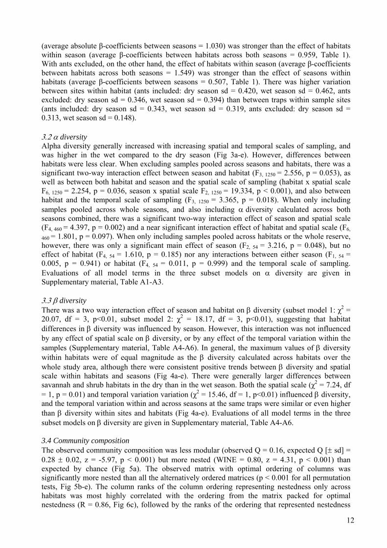
(average absolute β-coefficients between seasons = 1.030) was stronger than the effect of habitats within season (average β-coefficients between habitats across both seasons = 0.959, Table 1). With ants excluded, on the other hand, the effect of habitats within season (average β-coefficients between habitats across both seasons = 1.549) was stronger than the effect of seasons within habitats (average β-coefficients between seasons = 0.507, Table 1). There was higher variation between sites within habitat (ants included: dry season sd = 0.420, wet season sd = 0.462, ants excluded: dry season sd = 0.346, wet season sd = 0.394) than between traps within sample sites (ants included: dry season sd = 0.343, wet season sd = 0.319, ants excluded: dry season sd = 0.313, wet season sd = 0.148). diversity Alpha diversity generally increased with increasing spatial and temporal scales of sampling, and was higher in the wet compared to the dry season (Fig 3a-e). However, differences between habitats were less clear. When excluding samples pooled across seasons and habitats, there was a significant two-way interaction effect between season and habitat (F3, 1250 = 2.556, p = 0.053), as well as between both habitat and season and the spatial scale of sampling (habitat x spatial scale F6, 1250 = 2.254, p = 0.036, season x spatial scale F2, 1250 = 19.334, p < 0.001), and also between habitat and the temporal scale of sampling (F3, 1250 = 3.365, p = 0.018). When only including samples pooled across whole seasons, and also including diversity calculated across both seasons combined, there was a significant two-way interaction effect of season and spatial scale (F4, 460 = 4.397, p = 0.002) and a near significant interaction effect of habitat and spatial scale (F6,

460 = 1.801, p = 0.097). When only including samples pooled across habitats or the whole reserve, however, there was only a significant main effect of season (F2, 54 = 3.216, p = 0.048), but no effect of habitat (F4, 54 = 1.610, p = 0.185) nor any interactions between either season (F1, 54 = 0.005, p = 0.941) or habitat (F4, 54 = 0.011, p = 0.999) and the temporal scale of sampling. Evaluations of all model terms in the three subset models on diversity are given in Supplementary material, Table A1-A3.

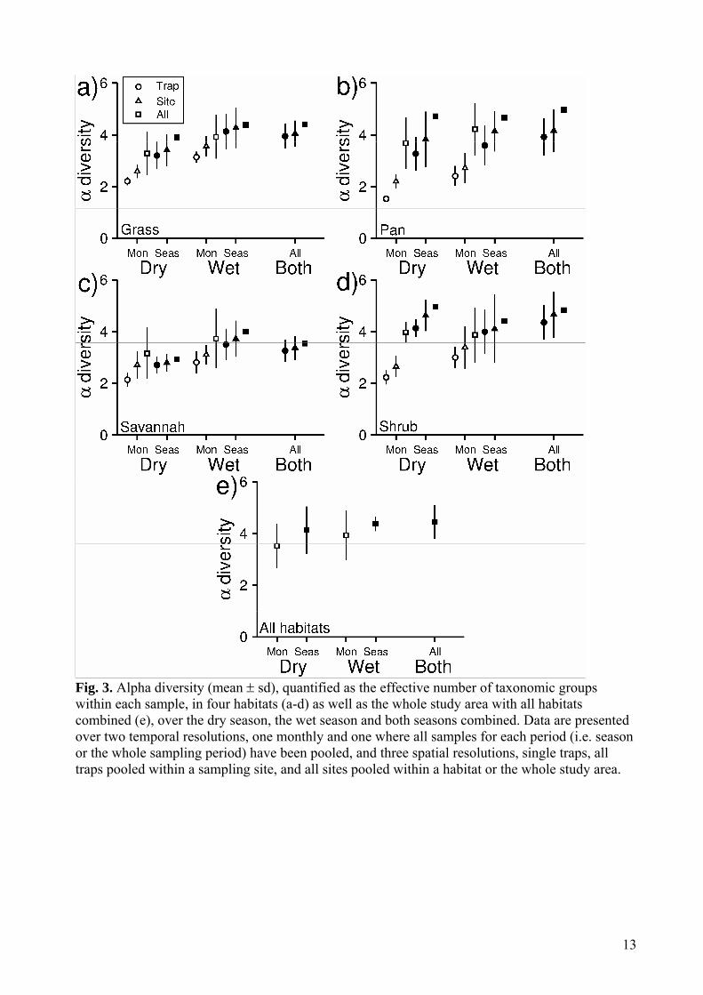
diversity There was a two way interaction effect of season and habitat on diversity (subset model 1: χ2 = 20.07, df = 3, p<0.01, subset model 2: χ2 = 18.17, df = 3, p<0.01), suggesting that habitat differences in diversity was influenced by season. However, this interaction was not influenced by any effect of spatial scale on diversity, or by any effect of the temporal variation within the samples (Supplementary material, Table A4-A6). In general, the maximum values of diversity within habitats were of equal magnitude as the diversity calculated across habitats over the whole study area, although there were consistent positive trends between diversity and spatial scale within habitats and seasons (Fig 4a-e). There were generally larger differences between savannah and shrub habitats in the dry than in the wet season. Both the spatial scale (χ2 = 7.24, df = 1, p = 0.01) and temporal variation variation (χ2 = 15.46, df = 1, p<0.01) influenced diversity, and the temporal variation within and across seasons at the same traps were similar or even higher than diversity within sites and habitats (Fig 4a-e). Evaluations of all model terms in the three subset models on diversity are given in Supplementary material, Table A4-A6.

3.4 Community composition The observed community composition was less modular (observed Q = 0.16, expected Q [ sd] = 0.28 0.02, z = -5.97, p < 0.001) but more nested (WINE = 0.80, z = 4.31, p < 0.001) than expected by chance (Fig 5a). The observed matrix with optimal ordering of columns was significantly more nested than all the alternatively ordered matrices (p < 0.001 for all permutation tests, Fig 5b-e). The column ranks of the column ordering representing nestedness only across habitats was most highly correlated with the ordering from the matrix packed for optimal nestedness (R = 0.86, Fig 6c), followed by the ranks of the ordering that represented nestedness

13

Fig. 3. Alpha diversity (mean sd), quantified as the effective number of taxonomic groups within each sample, in four habitats (a-d) as well as the whole study area with all habitats combined (e), over the dry season, the wet season and both seasons combined. Data are presented over two temporal resolutions, one monthly and one where all samples for each period (i.e. season or the whole sampling period) have been pooled, and three spatial resolutions, single traps, all traps pooled within a sampling site, and all sites pooled within a habitat or the whole study area.

14

Fig. 4. Beta diversity (mean SE), quantified as Euclidean distances from each trap to centroids in a multivariate space defined by the taxonomic group of arthropods. Centroids have been calculated across four spatial scales, trap (which lacks spatial resolution and hence only reflects temporal variation within and across seasons), site, habitat and the whole reserve, and three temporal scales, month (a,b), season (c,d) and both seasons combined (e).

15

Fig. 5. Graphic representations of observed (a) and expected interaction matrices for four competing hypotheses regarding nested community composition: b) communities are nested across habitats and within each habitat also across seasons, c) communities are nested across seasons and within each season also across habitats, d) Communities are only nested across habitats, and e) communities are only nested across seasons. In all matrices the taxon groups are ordered according to occurrence. In the observed matrix, the columns are ordered according to occurrences (i.e. this matrix represent the most nested pattern derived from the data), whereas in the expected matrices the columns are ordered first by respective habitat and season class, and within each relevant class ordered according to occurrences. Both habitats and season were ordered based on total number of occurrences. Darker shades represent more trapped individuals.

16

Fig. 6. Correlation between the observed rank of sites ordered by maximum abundance and orders reflecting four competing hypotheses regarding nested community composition: a) communities are nested across habitats and within each habitat also across season, b) communities are nested across season and within each season also across habitats, c) Communities are only nested across habitats, and d) communities are only nested across seasons.

17

also across seasons within habitats (R = 0.80, Fig 6a). The ranks of the ordering representing nestedness only across seasons (R = 0.59) and nestedness across seasons and within each season across habitats (R = 0.52) were not as highly correlated to the ranks of the optimally ranked matrix (Fig 6b,d).

4. Discussion

Our results indicated that local processes and seasonal variation in climate interacted in shaping local arthropod communities, both in terms of abundance and taxonomic composition. We found increased arthropod abundance in the wet compared to the dry season. This result agrees with previous suggestions that seasonal variation of arthropod communities in arid grassland and savannah regions are mainly caused by variation in rainfall (Wolda 1988), although we can not rule out that seasonal variation in temperature was influential as well. Climate mediated effects in temporal variation in arthropod communities may primarily be related to seasonal differences in plant growth, with subsequent differences in availability of food and of refugia (O'Connor 1994, Milton and Dean 2000).

Contrary to our predictions, we did not find that community structures were specific to each habitat, nor that communities sampled in the season with least arthropod abundance (i.e. the dry season) were nested within communities sampled within the season with the highest abundance (wet season). Instead, we found that the observed nested pattern more closely related to a spatial nestedness; communities sampled in less arthropod rich habitats seemed to be nested within communities sampled within more arthropod rich ones. Such nested distribution patterns are common across a wide range of ecosystems and taxonomic groups, and can be attributed to several factors (Wright et al. 1998). We suggest three possible explanations for these observations. Firstly, neutral assembly processes such as random dispersal could have shaped local communities within habitats, where the richer habitats could be regarded as source communities from which communities in the other habitats were drawn from (Chase and Mayers 2011). Secondly, heterogeneity within rather than across habitats could have shaped the observed lack of modular structures, and possibly also cause the spatial nestedness. Contrary to the previous suggestion, this would suggest some level of niche related process (Chesson 2000), albeit at a finer spatial scale than the broad habitat classes we used here. Thirdly, our lack of observed modularity could have been an artefact (sensu Palmer et al. 2008) caused by our coarse taxonomic resolution. In such a case, any community differentiation would have been observed at finer taxonomic resolutions than the one we used. Such an interpretation would similarly imply a niche based assembly process, since any effects of taxonomic scale should have been mediated by a taxonomic scaling of traits associated with niche utilization (Bevilacqua et al. 2012). However, we interpret our observed positive association between diversity and spatial scale as well as the similar diversity within and across habitats as support for the importance of neutral processes in the formation of arthropod communities in this arid grassland (Chase et al. 2005).

We found that diversity increased with increased spatial and temporal scales of sampling. These results mirror previous suggestions that biodiversity has to be evaluated at multiple scales (Tylianakis et al. 2006). We observed a higher diversity in the season with the highest abundance (i.e. the wet season), which suggests that the temporal scale dependence may have been caused by a higher likelihood of sampling rare taxonomic groups at larger time scales (e.g., Gotelli and Colwell 2001). However, our results also suggest that both spatial and temporal scale dependence may have differed between habitats. Although we can not rule out confounding effects of sampling intensity, we believe that these observations highlight that assembly processes within habitats may have been highly influential in determining the composition of local arthropod communities, and that such processes may not necessarily have been neutral. Similar results have been found for vertebrates in a Mediterranean environment (Martin and Ferrer 2015). Contrary to recent claims that regional processes may be more important than local ones for the assembly of local ecological communities (Rickliefs 2008), we suggest that local processes are not only

18

directly important for the composition of local arthropod communities, but also that variation in such processes within and among habitats are critically important for how arthropods vary across time and space. We therefore accentuate the potential importance of maintaining heterogeneity even within habitats for the maintenance of biodiversity at a range of spatial and temporal scales.

We found that diversity appeared to be of the same magnitude if quantified across time or across space. Moreover, we did not find any evidence for a temporal nestedness in the observed arthropod communities. The level of diversity is predicted to be positively related to the level of environmental specialization, with high diversity being caused by high levels of specialization to local environmental conditions (Jankowski et al. 2009). Our results therefore suggest that adaptation to climate related factors may be as important as adaptations to habitat related factors, and subsequently that alterations in climate may have profound influences on the patterns of biodiversity. Such suggestions are not novel (Parmesan and Yohe 2003, Hillebrand et al. 2010), but highlight that alterations in climate and associated seasonal characteristics may have broad scale consequences across a wide range of relevant ecological scales.

We conducted the study with a coarse taxonomic resolution. Although such coarse resolution may have confounded the results, e.g. it has been suggested that spatial nestedness increases with decreasing taxonomic resolution (Wright et al. 1998), arthropod diversity at coarse taxonomic resolutions have been found to correspond to diversity at finer resolutions (Williams and Gaston 1994, Vanderklift et al. 1998, Báldi 2003, Bang and Faeth 2011), and diversity patterns have been suggested as robust against taxonomic resolution (Storch and Sizling 2008). We suggest that maintaining larger taxonomic groupings was beneficial in that it allowed us to keep robust taxonomic classifications without being influenced by the relative taxonomic uncertainty between groups, and hence avoid issues related to the taxonomic accuracy of the included taxa (Jones 2008). Fine scale taxonomic resolutions may also have introduced a large number of empty cells in our data matrices, which could have had serious consequences for analytical results (Galeano et al. 2009, Heino et al. 2015). Alternatives could be to pool data either across time or space, but by maintaining a coarse taxonomic resolution we were instead able to address questions related to a wider range of both spatial and temporal scales, which we believe was instrumental for maintaining appropriate ecological focus for our questions. Hence, although we call for caution in generalizing our results to other taxonomic scales, we believe that our study still has been informative in evaluating the relative effects of spatial variation within and between habitats, as well as temporal variation related to seasonal variation primarily in rainfall, on local arthropod communities in this arid environment.

To conclude, our result supported previous studies suggesting seasonal climate variation, probably strongly linked to rainfall, as a major driver of arthropod abundance, but in our study area such climate effects appeared to have differed between habitats. We found evidence for spatial nestedness in arthropod communities. However, communities were no not completely nested across either habitats or seasons. We also observed that diversity was positively associated with spatial scale within habitats and was as high within as across habitats. We interpret these observations as support for the importance of neutral processes for shaping arthropod community structure. However, both spatial and temporal scale dependence of diversity differed among habitats, which suggest that processes acting at very local scales may also have been important for arthropod diversity, and that such process may have been related to non-neutral processes. Finally, we found that diversity appeared to be as high across seasons as across and within habitats, which points to the potential for climate alterations to substantially affect arthropod diversity in this arid region.

Acknowledgements We are most grateful to the numerous field assistants that aided with field data collection. This research was conducted with the kind permission by De Beers Mining Corporation to conduct research on Benfontein Game Reserve, and we are grateful for the logistic support they offered on the reserve. We are most grateful to Professor Nigel C. Bennett for assistance with various parts

19

of this research. The research was financially supported by a South African Research Chair Initiative chair of Mammal Behavioural Ecology and Physiology awarded by the National Research foundation (NRF) to N.C. Bennett, an NRF Focus Area grant awarded to E.Z. Cameron, P.W Bateman and F. Dalerum, NRF and University of Pretoria incentive funding awarded to F. Dalerum and C.W.W. Pirk and a Ramòn y Cajal fellowship awarded to F. Dalerum by the Spanish Ministry of Competitiveness and Economy.

References Alonso, D., Etienne, R. S., McKane, A. J. 2006. The merits of neutral theory. -Tr. Ecol. Evol. 21:

451-457. Anderson, M. J., Crist, T. O., Chase, J. M., Vellend, M., Inouye, B. D., Freestone, A. L., Sanders,

N. J., Cornell, H. V., Comita, L. S., Davies, K. F., Harrison, S. P., Kraft, N. J. B., Stegen, J. C., Swenson, N. G. 2011. Navigating the multiple meanings of diversity: a roadmap for the practicing ecologist. -Ecol. Lett. 14: 19-28.

Anderson, M. J., Ellingsen, K. E. and McArdle, B. H. 2006. Multivariate dispersion as a measure of beta diversity. - Ecol. Lett. 9: 683-693.

Báldi, A. 2003. Using higher taxa as surrogates of species richness: a study based on 3700 Coleoptera, Diptera, and Acari species in Central-Hungarian reserves. -Basic Appl. Ecol. 4: 589-593.

Bang, C., Faeth, S. H. 2011. Variation in arthropod communities in response to urbanization: Seven years of arthropod monitoring in a desert city. - Landsc. Urb. Plan. 103: 383-399.

Bates, D., Maechler, M., Bolker, B., Walker, S. 2014. lme4: Linear mixed-effects models using Eigen and S4. -ArXiv 1406.5823.

Bevilacqua, S., Terlizzi, A., Claudet, J., Fraschetti, S., Boero, F. 2011. Taxonomic relatedness does not matter for species surrogacy in the assessment of community responses to environmental drivers. -J. Appl. Ecol. 49: 357-366.

Borthagaray, A. I., Arim, M., Marquet, P. A. 2014. Inferring species roles in metacommunity structure from species co-occurrence networks. -Proc. Roy. Soc. B: Biology 281: 1792.

Cagnolo, L., Molina, S.I., Valladares, G. R. 2002. Diversity and guild structure of insect assemblages under grazing and exclusion regimes in a montane grassland from Central Argentina. -Biodiv. Cons. 11: 407-420.

Cardinale, B. J., Duffy, J. E., Gonzalez, A., Hooper, D. U., Perrings, C., Venail,P., Narwani, A., Mace, G. M., Tilman, D., Wardle, D. A., Kinzig, A. P., Daily, G. C., Loreau, M., Grace, J. B., Larigauderie, A., Srivastava, D. S., Naeem, S. 2012. Biodiversity loss and its impact on humanity. Nature 486: 59-67.

Chase, J. M., Amarasekare, P., Cottenie, K., Gonzalez, A., Holt, R. D., Holyoak, M., Hoopes, M. F., Leibold, M. A., Loreau, M., Mouquet, N., Shurin, J. B., Timlan, D. 2005. Competing theories for competitive metacommunities. -In Holyoak, M., Leibold, M. A., Holt, R. D. (eds), Metacommunities: spatial dynamics and ecological communities. University of Chicago Press, pp. 335–354.

Chase, J. M., Mayers, J. A. 2011. Disentangling the importance of ecological niches from stochastic processes across scales. -Phil. Trans. Roy. Soc. B 366: 2351-2363.

Chesson, P. 2000. Mechanisms of maintenance of biodiversity. –Ann. Rev. Ecol. Evol. 31: 343-366.

Crist, T. O., Veech, J. A. Gering, J. C., Summerville, K. S. 2003. Partitioning species diversity across landscapes and regions: a hierarchical analysis of a, b and g diversity. -Am. Nat. 162: 734–743.

Cook, R. R., Quinn, J. F. 1995. The influence of colonization in nested species subsets. -Oecologia 102: 413-424.

DeVries, P. J., Murray, D. Lande, R. 1997. Species diversity in vertical, horizontal, and temporal dimensions of a fruit-feeding butterfly community in an Ecuadorian rainforest. -Biol. J. Linn. Soc. 62: 343–364.

20

Dormann C. F., Fruend J., Bluethgen N., Gruber, B. 2009. Indices, graphs and null models: analyzing bipartite ecological networks. -Open Ecol. J. 2: 7-24.

Dormann, C. F., Strauss, R. 2014.A method for detecting modules in quantitative bipartite networks. -Meth. Ecol. Evol. 5: 90-98.

Ellis, D. 1985. Taxonomic sufficiency in pollution assessment. -Mar. Poll. Bull. 16: 442–461. Galeano, J., Pastor, J. M., Iriondo, J. M. 2009. Weighted-Interaction Nestedness Estimator

(WINE): A new estimator to calculate over frequency matrices. -Env. Mod. Softw. 24: 1342-1346.

Gering, J. C., Crist, T. O., Veech, J. A. 2003. Additive partitioning of species diversity across multiple spatial scales: implications for regional conservation of biodiversity. -Cons. Biol. 17: 488-499.

Gibson, R. H., Knott B., Eberlein, T., Memmot J. 2011. Sampling method influences the structure of plant-pollinator networks. -Oikos 120: 822-831.

Gotelli, N. J., Colwell, R. K. 2001. Quantifying biodiversity: procedures and pitfalls in the measurement and comparison of species richness. -Ecol. Lett. 4: 379-391.

Hawkins, B. A., Field, R., Cornell, H. V., Currie, D. J., Guegan, J. F., Kaufman, D. M., Kerr, J. T., Mittelbach, G. G., Oberdorff, T., O’Brien, E. M., Porter, E. E., Turner, J. R. G. 2003. Energy, water, and broad-scale geographic patterns of species richness. Ecology 84: 3105-3117.

Hector, A., von Felten, S., Schmid, B. 2010. Analyses of variance with unbalanced data: an update for ecology and evolution. -J. Anim. Ecol. 79: 308-316.

Heino, J., Melo, A. S., Bini, L. M.. Altermatt, F., Al-Shami, S. A., Angeler, D. G., Bonada, N., Brand, C., Callisto, M., Cottenie, K., Dangles, O., Dudgeon, D., Encalada, A., Gothe, E., Gronroos, M., Hamada, N., Jacobsen, D., Landeiro, V. L., Ligeiro, R., Martins, R. T., Miserendino, M. L., Md Rawi, C. S., Rodrigues, M. E., Roque, F. D., Sandin, L., Schmera, D., Sgarbi, L. F., Simaika, J. P., Siqueira, T., Thompson, R. M., Townsend, C. R. 2015. A comparative analysis reveals weak relationships between ecological factors and beta diversity of stream insect metacommunities at two spatial levels. Ecol. Evol. 5: 1235-1248.

Hillebrand, H. 2004. On the generality of the latitudinal diversity gradient. Am. Nat. 163: 192-211.

Hillebrand, H., Soininen, H., Snoeijs, H. 2010. Warming leads to higher species turnover in a coastal ecosystem. -Glob. Ch. Biol. 16: 1181-1193.

Hothorn, T., Brets, F., Westfall, P. 2008. Simultaneous inference in general parametric models. Biometr. J. 50: 346-363.

Hooper, D. U., Chapin, F. S. I., Ewel, J. J., Hector, A., Inchausti, P., Lavorel, S., Lawton, J. H., Lodge, D. M., Loreau, M., Naeem, S., Schmid, B., Setälä, H., Symstad, A. J., Vandermeer, J., Wardle, D. A. 2005. Effects of biodiversity on ecosystem functioning:a consensus of current knowledge. - Ecol. Monogr. 75: 3-35.

Hooper, D. Buchmann, N., Degrange, V, Díaz, S. M. Gessner, M. O. Grime, P., Hulot, F., Mermillod-Blondin, F., van Peer, L., Roy, J., Symstad, A., Solan, M., Spehn, E. M. 2002. Species diversity, functional diversity and ecosystem functioning. -In Loreau, M., Naeem, S., Inchausti, P. (eds), Biodiversity and ecosystems functioning: a current synthesis. Oxford Univ. Press, pp. 195-208.

Hubbell, S. 2001. The unified theory of biodiversity and biogeography. -Princeton University Press.

Hultèn, E. 1937. Outline of the history of Arctic and Boreal biota during the Quaternary period. -Thule.

Jankowski, J., Ciecka, A., Meyer, N., Rabenold, K. 2009. Beta diversity along environmental gradients: implications of habitat specialization in tropical montane landscapes. -J. Animal Ecol. 78: 315-327

Jones, F. C. 2008. Taxonomic sufficiency: The influence of taxonomic resolution on freshwater bioassessments using benthic macroinvertebrates. -Env. Rev. 16: 45-69.

21

Jost, L. 2006. Entropy and diversity. -Oikos 113: 363-375. Kotze, R., Pirk, C. W. W., Bennett, N. C., Cameron, E. Z., De Vries, J. L., Marneweck, D.,

Dalerum, F. 2012. Temporal patterns of den use suggest polygamous mating patterns in an obligate monogamous mammal. -Anim. Behav. 84: 1573-1578.

Lande, R. 1996. Statistics and partitioning of species diversity, and similarity among multiple communities. -Oikos 76: 5-13.

Lawton, J. H., Bignell, D. E., Bolton, B., Bloemers, G. F., Eggleton, P., Hammond, P. M., Hodda, M., Holt, R. D., Larsen, T. B., Mawdseley, N. A., Stork, N. E., Srivastava, D. S., Watt, A. D. 1998. Biodiversity inventories, indicator taxa and effects of habitat modification in tropical forests. -Nature 391: 72-76.

Martin, B., Ferrer, M. 2015. Temporally variable environments maintain more beta-diversity in Mediterranean landscapes. -Acta Oecol. 68: 1-10.

Manly, B. F. J. 1997. Randomization, bootstrap, and Monte Carlo methods in biology. 2nd ed. -Chapman and Hall.

Maindonald, J. H., Braun, W. J. 2015. DAAG: Data analysis and graphics data and functions. R package version 1.22. http://cran.r-project.org/package=DAAG

McGeogh, M. A. 1998. The selection, testing and application of terrestrial insects as bioindicators. -Biol. Rev. 73: 181-201.

Miranda, M., Parrini, F., Dalerum, F. 2013. A categorization of network approaches to analyse trophic relationships. Meth. Ecol. Evol. 4: 897-905.

Milton, S. J., Dean, W. R. J. 2000. Disturbance, drought and dynamics of desert dune grassland, South Africa. -Pl. Ecol. 150: 37-51.

O'Connor, T. G. 1994. Composition and population responses of an African savanna grassland to rainfall and grazing. -J. Appl. Ecol. 31: 155-171.

Ødegaard, F. 2000. How many species of arthropods? Erwin’s estimate revised. -Biol. J. Linn. Soc. 71: 583–597.

Oksanen, J., Blanchet, F.G., Kindt, R., Legendre, P., Minchin, P. R., O'Hara, R. B., Simpson, G. L., Solymos, P., Stevens, M. H. H., Wagner H. 2015. vegan: Community ecology package. R package version 2.2-1. http://cran.r-roject.org/package=vegan

Olesen, J. M. Bascompte, J. Dupont, Y .L., Jordano, P. 2007. The modularity of pollination networks. -Proc. Nat. Acad. Sci. 104: 19891-19896.

Palmer, M. W., McGlinn, D. J., Fridley, J. A. 2008. Artefacts and artifictions in biodiversity research. Folia Geobot. 43: 245-257.

Parmesan, C., Yohe G. 2003. A globally coherent fingerprint of climate change impacts across natural systems. -Nature 421: 37-42.

Pimm, S. L. 1982. Food webs. -Chicago Univ. Press. Reiss, J., Bridle, J. R., Montoya, J. M., Woodward, G. 2009. Emerging horizons in biodiversity

and ecosystem functioning research. Tr. Ecol. Evol. 24: 505-514. Richardson, P. R. K. 1985. The social behaviour and ecology of the aardwolf, Proteles cristatus

(Sparrman, 1783) in relation to its food resources. PhD Dissertation, Univ. of Oxford. Rickliefs, R. E. 2008. Disentigration of the ecological community. -Am- Nat. 172: 741-750. Rollin, O., Bretagnolle, V., Fortel, L., Guilbaud, L., Henry, M. 2015. Habitat, spatial and temporal

drivers of diversity patterns in a wild bee assemblage. –Biodiv. Cons. 24: 1195-1214. Rosensweig, M. L. 1995. Species diversity in time and space. -Cambridge Univ. Press. Schulze, R. E., McGee, O. S. 1978. Climatic indices and classification in relation to the

biogeography of southern Africa. In: Werger M. J. A. and B. A. C. (eds), Biogeography and ecology of Southern Africa. Junk Publ., pp. 21–52.

Shannon, C. E. 1948. A mathematical theory of communication. -Bell Syst. Techn. J. 27: 379-423. Siemann, E., Tilman, D., Haarstad, J., Ritchie M. 1998. Experimental tests of the dependence of

arthropod diversity on plant diversity. -Am. Nat. 152: 738-750. Slipinski, P., Zmihorski, M., Czechowski, W. 2012. Species diversity and nestedness of ant

assemblages in an urban environment. -Eur. J. Entomol. 109: 197-206.

22

Southwood, T. R. E., Brown, V. K., Reader P. M. 1979. The relationships of plant and insect diversities in succession. -Biol. J. Linn. Soc. 12: 327-348.

Storch, D., Šizling, A. L. 2008. The concept of taxon invariance in ecology: do diversity patterns change with changes in taxonomic resolution? -Folia Geobot. 43: 329-344.

Summerville, K. S., Crist, T. O. 2005. Temporal patterns of species accumulation in a survey of Lepidoptera in a beech–maple forest. Biodiv. Cons. 14: 3393-3406.

Thèbault, E. 2013. Identifying compartments in presence–absence matrices and bipartite networks: insights into modularity measures. -J. Biogeogr. 40: 759-768

Tylianakis, J., Klein, A. M., Lozada, T., Tscharntke, T. 2006. Spatial scale of observation affects a, b and g diversity of cavity-nesting bees and wasps across a tropical land-use gradient. -J. Biogeogr. 33: 1295-1304.

Tylianakis, J., Klein, A. M., Tscharntke, T. 2005. Spatiotemporal variation in the diversity of hymenoptera across a tropical habitat gradient. Ecology 86: 3296-3302.

Ulrich, W., Almeida-Neto, M. and Gotelli, N. J. (2009) A consumers guide to nestedness analysis. -Oikos 118: 3-17.

Ulrich ,W. and Gotelli, N. L. 2007. Null model analyses of species nestedness patterns. -Ecology 88: 1824-1831.

van Rijn, I., Neeson, T. M., Mandelik, Y. 2015. Reliability and refinement of the higher taxa approach for bee richness and composition assessments. Ecol. Appl. 25: 88-98.

Walker, M., Jones, T. H. 2001. Relative roles of top-down and bottom-up forces in terrestrial tritrophic plant–insect herbivore–natural enemy systems. -Oikos 93: 177-187.

Williams, P. H., Gaston, K. J. 1994. Measuring more of biodiversity: Can higher taxon-richness predict wholesale species richness? -Biol. Cons. 67: 211-217.

Wolda, H. 1988. Insect Seasonality: Why? -Ann. Rev. Ecol. Syst. 19: 1-18.