spatial analyst - suitability modeling - esri...the suitability modeling model steps • determine...

ArcGIS Spatial Analyst – Suitability Modeling

Kevin M. Johnston Elizabeth Graham

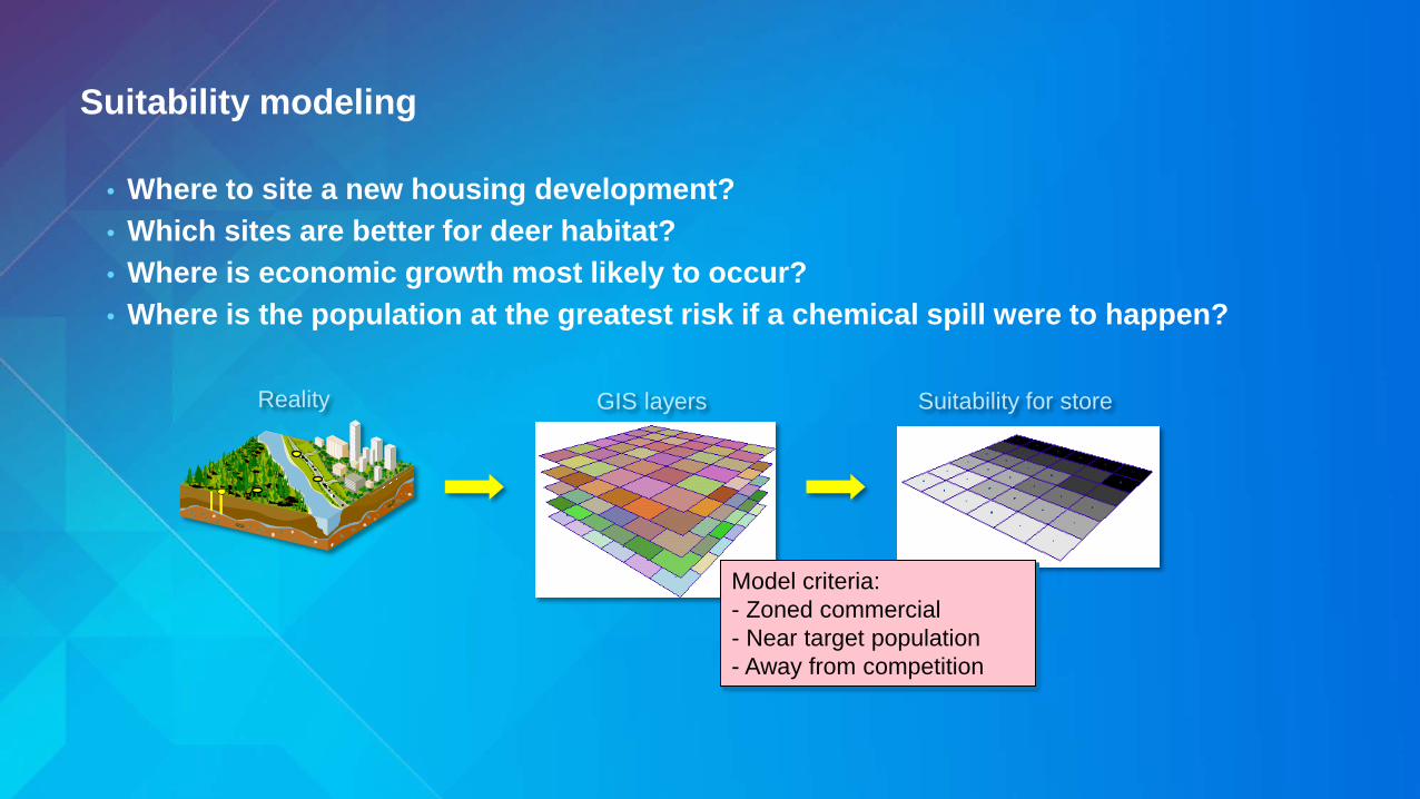
Suitability modeling

• Where to site a new housing development? • Which sites are better for deer habitat? • Where is economic growth most likely to occur? • Where is the population at the greatest risk if a chemical spill were to happen?

Reality GIS layers Suitability for store

Model criteria: - Zoned commercial - Near target population - Away from competition

What we know

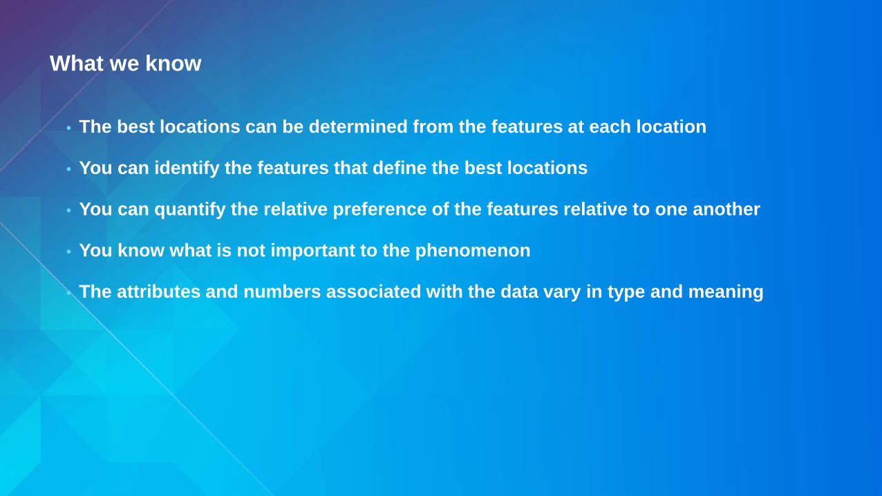
• The best locations can be determined from the features at each location

• You can identify the features that define the best locations

• You can quantify the relative preference of the features relative to one another

• You know what is not important to the phenomenon

• The attributes and numbers associated with the data vary in type and meaning

The presentation outline

• Background

• How to create a suitability model and the associated issues

• Demonstration

• Look deeper into the transformation values and weights

• Demonstration

• Fuzzy logic

Manipulation of raster data - Background

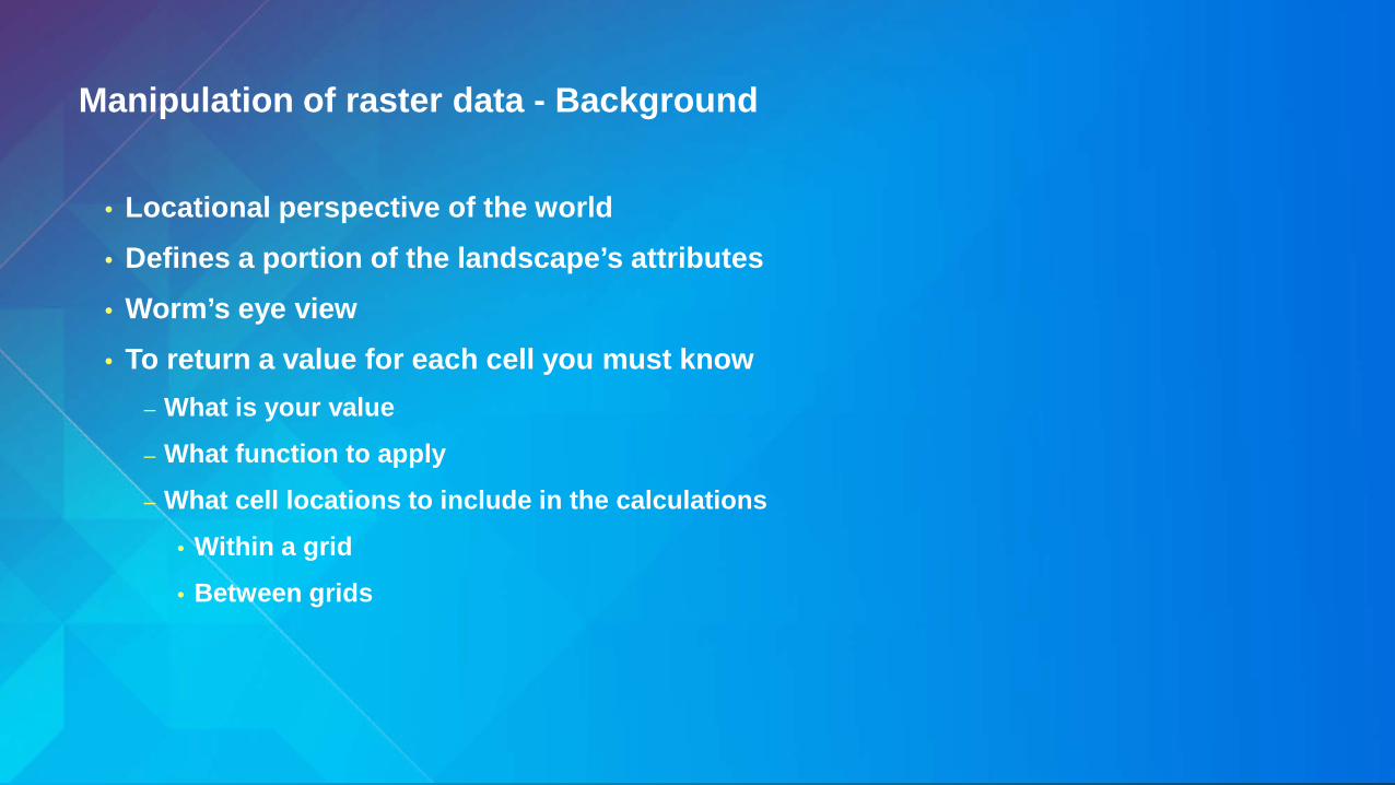
• Locational perspective of the world • Defines a portion of the landscape’s attributes • Worm’s eye view • To return a value for each cell you must know

– What is your value

– What function to apply

– What cell locations to include in the calculations

• Within a grid

• Between grids

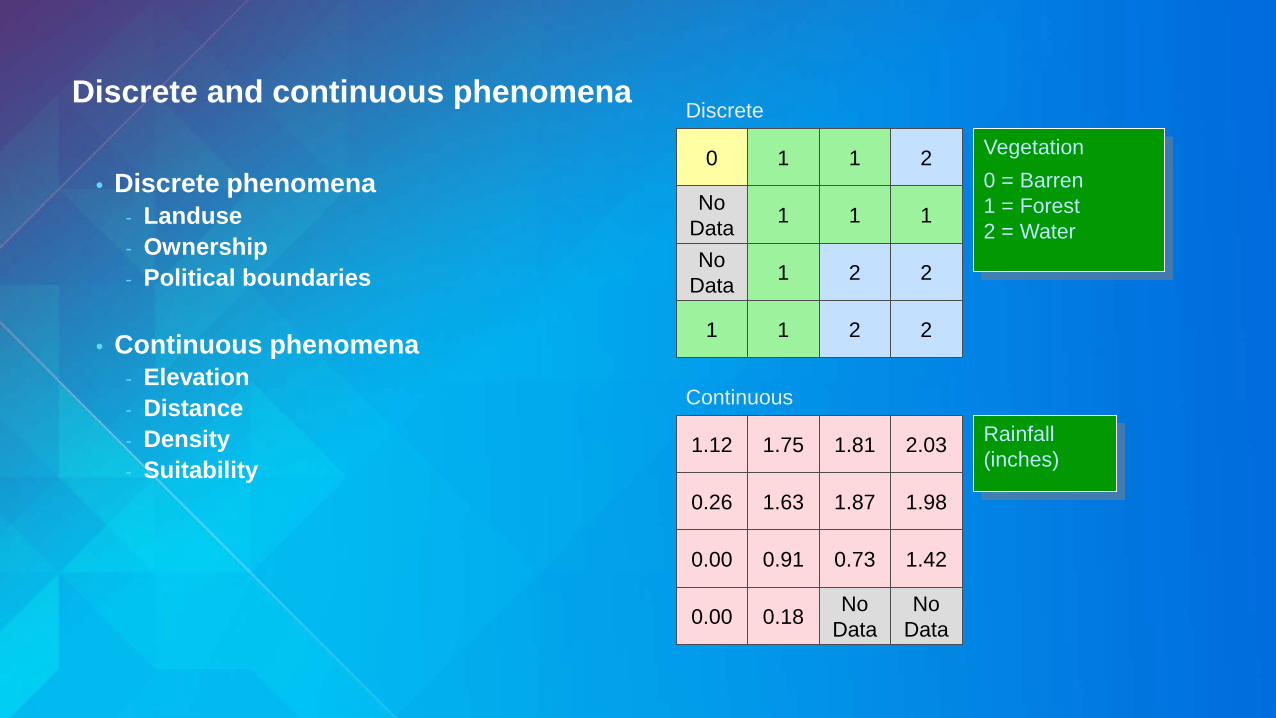
Discrete and continuous phenomena

• Discrete phenomena - Landuse - Ownership - Political boundaries

• Continuous phenomena

- Elevation - Distance - Density - Suitability

2 1 1 0

No Data 1 1 1

No Data 1 2 2

1 1 2 2

Vegetation 0 = Barren 1 = Forest 2 = Water

Discrete

1.12 1.75 1.81 2.03

0.26 1.63 1.87 1.98

0.00 0.91 0.73 1.42

0.00 0.18 No Data

No Data

Rainfall (inches)

Continuous


• Background


• Demonstration


• Demonstration

• Fuzzy logic

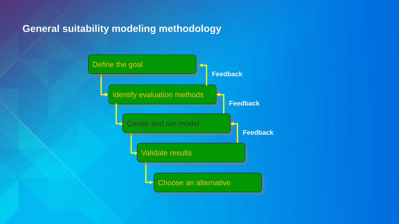
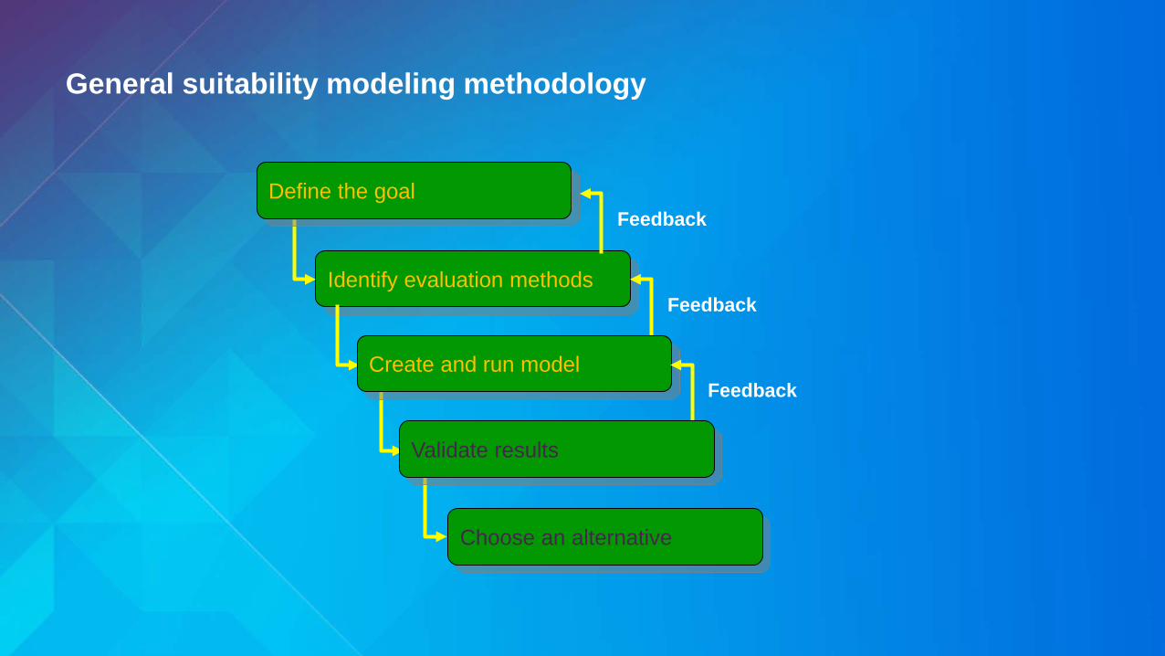
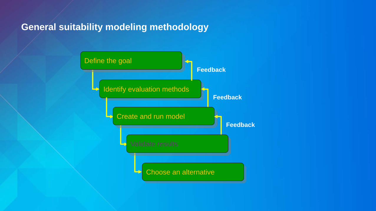
General suitability modeling methodology

Identify evaluation methods

Feedback

Feedback

Define the goal

Create and run model

Choose an alternative

Feedback

Validate results

Problem definition

• Most important and most time consuming – glossed over • Measurable • The gap between desired and existing states

• Define the problem

• “Locate a ski resort”

• Establish the over arching goal of the problem • Make money

• Identify issues • Stakeholders

• Legal constraints

Models and sub-models

• Break down problem into sub models - Helps clarify relationships, simplifies problem

Terrain Sub-model

Development Cost Sub-model

Input Data (many)

Accessibility Sub-model

Ski Resort Model

Best Resort Sites

Input Data (many)

Input Data (many)


• How will you know if the model is successful?

• Criteria should relate back to the overall goals of the model

• May need to generalize measures • “On average near the water”

• Determine how to quantify • “Drive time to the city”

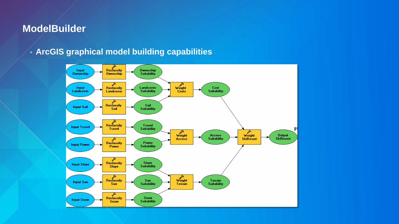
ModelBuilder

• ArcGIS graphical model building capabilities

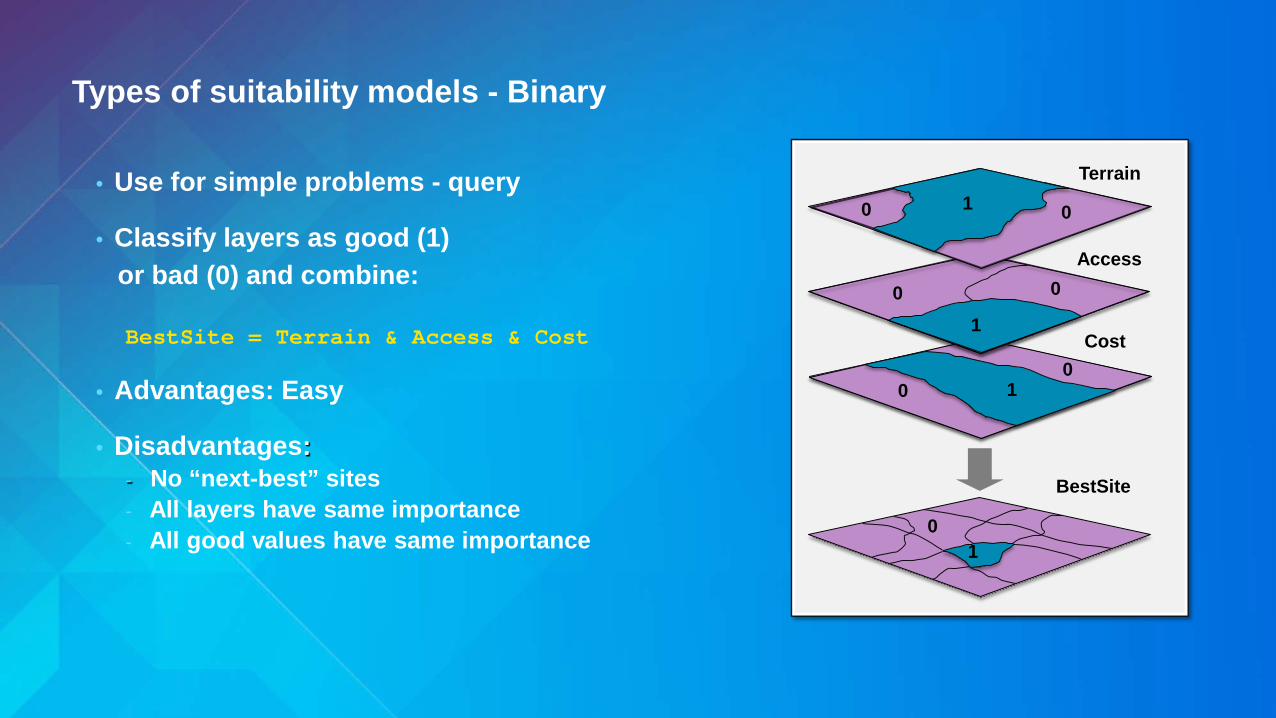
Types of suitability models - Binary

• Use for simple problems - query

• Classify layers as good (1) or bad (0) and combine:

BestSite = Terrain & Access & Cost

• Advantages: Easy

• Disadvantages: - No “next-best” sites - All layers have same importance - All good values have same importance

Access

Cost

BestSite

Terrain

0

0 0

1

0 1 0

0 1

1 0

1

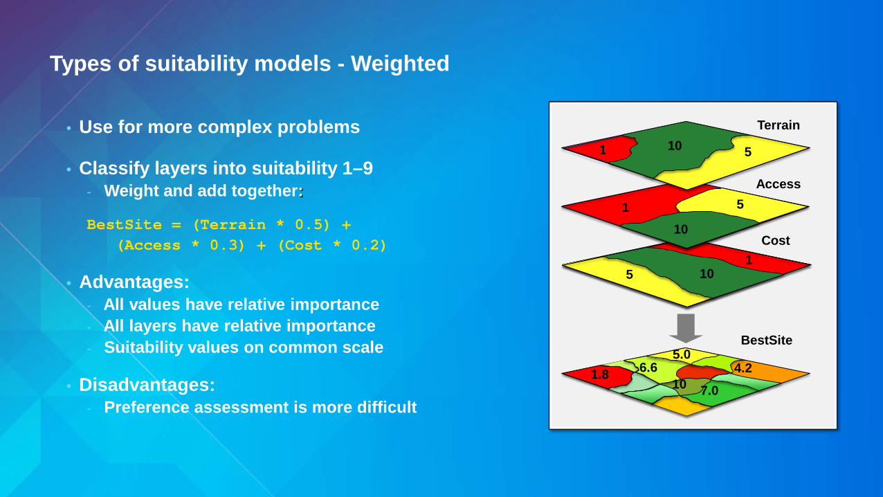
Types of suitability models - Weighted

• Use for more complex problems

• Classify layers into suitability 1–9 - Weight and add together:

BestSite = (Terrain * 0.5) + (Access * 0.3) + (Cost * 0.2)

• Advantages: - All values have relative importance - All layers have relative importance - Suitability values on common scale

• Disadvantages: - Preference assessment is more difficult

Access

Cost

BestSite

Terrain

1

1

5 10

5

5

10

1 10

10 6.6

7.0

4.2 5.0

1.8



Feedback

Feedback

Define the goal



Feedback

Validate results

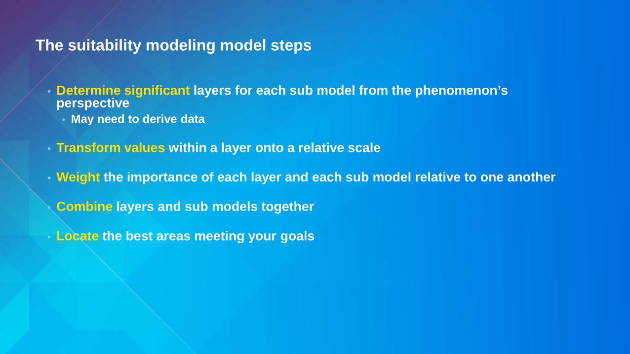
The suitability modeling model steps

• Determine significant layers for each sub model from the phenomenon’s perspective

• May need to derive data

• Transform values within a layer onto a relative scale

• Weight the importance of each layer and each sub model relative to one another

• Combine layers and sub models together

• Locate the best areas meeting your goals

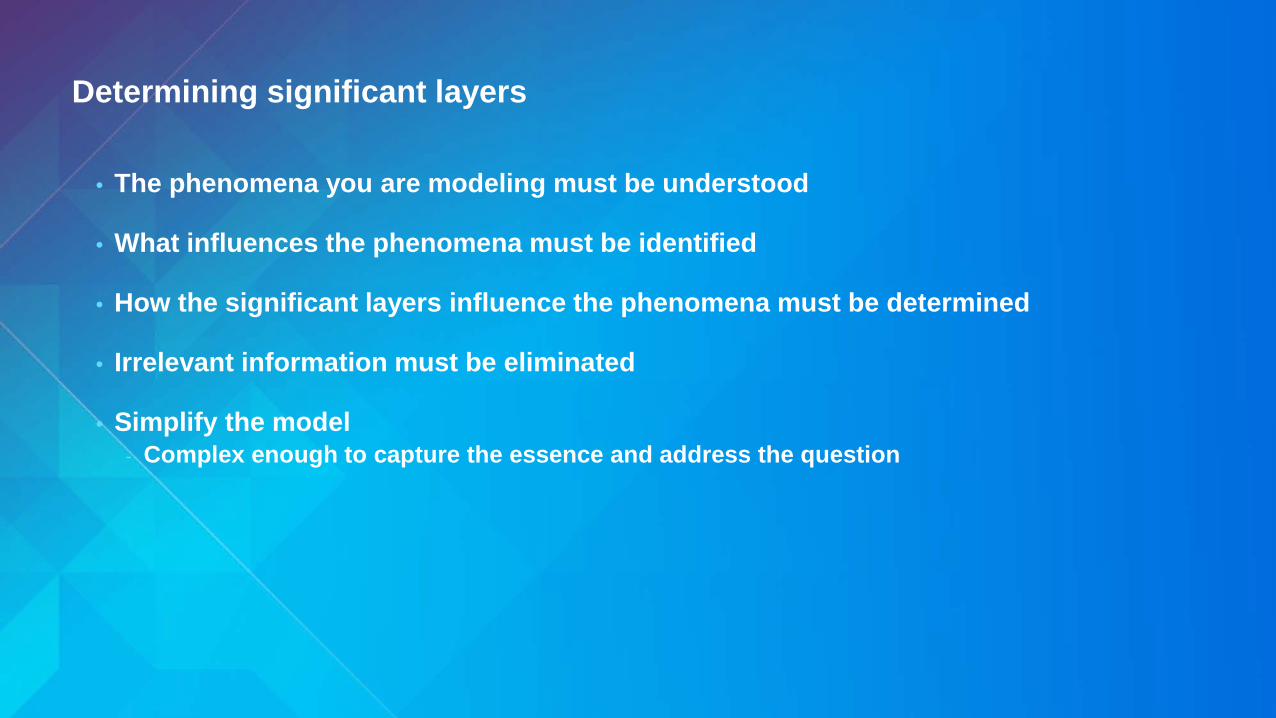
Determining significant layers

• The phenomena you are modeling must be understood

• What influences the phenomena must be identified

• How the significant layers influence the phenomena must be determined

• Irrelevant information must be eliminated

• Simplify the model - Complex enough to capture the essence and address the question

Transform values – Place various criteria on common scale

• Base data may not be useful for measuring all criteria

- Need to measure access, not road location

• May be easy: - ArcGIS Spatial Analyst tools - Distance to roads

• May be harder: - Require another model - Travel time to roads

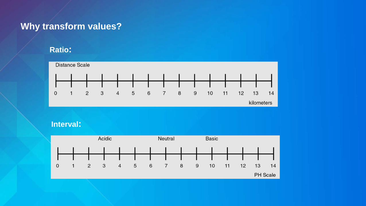
Why transform values?

Ratio:

Interval:

Why transform values?

Nominal: Ordinal:

Transform values – Define a scale of suitability

• Define a scale for suitability - Many possible; typically 1 to 9 (worst to best) - Reclassify layer values into relative suitability - Use the same scale for all layers in the model

Travel time suitability

8 7 6 5 – 15 minutes to off ramp 4 3 2

9 – 0 minutes to off ramp

1 – 45 minutes to off ramp

Best

Worst

Soil grading suitability

8 7 6

5 – Landslide; moderate 4 3 2

9 – Recent alluvium; easy

1 – Exposed bedrock; hard

Best

Worst

0

3282.5

Distance to roads

9

7

8

6 5

Suitability for Ski Resort Within and between layers

Accessibility sub model Development sub model

Tools to transform your values – convert to suitability

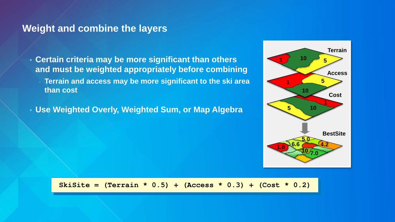
Weight and combine the layers

• Certain criteria may be more significant than others and must be weighted appropriately before combining

- Terrain and access may be more significant to the ski area than cost

• Use Weighted Overly, Weighted Sum, or Map Algebra

SkiSite = (Terrain * 0.5) + (Access * 0.3) + (Cost * 0.2)

Access

Cost

BestSite

Terrain 1

1

5 10

5

5

10

1 10

10 6.6

7.0 4.2

5.0 1.8

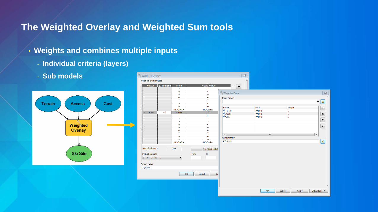
The Weighted Overlay and Weighted Sum tools

• Weights and combines multiple inputs - Individual criteria (layers)

- Sub models

Locate

• Model returns a suitability “surface” - Ranks the relative importance of each site to one another

relative to the phenomenon

• Create candidate sites - Select cells with highest scores - Define regions with unique IDS (Region Group) - Eliminate regions that are too small

• Choose between the candidates

Site 1

Site 2

Site 3


• Background


• Demonstration


• Demonstration

• Fuzzy logic

Demo Basic Suitability Model Transform values Weight Combine



Feedback

Feedback

Define the goal



Feedback

Validate results

Validation

• Ground truth – visit the site in person

• Use local knowledge and expert experience

• Alter values and weights

• Perform sensitivity and error analysis

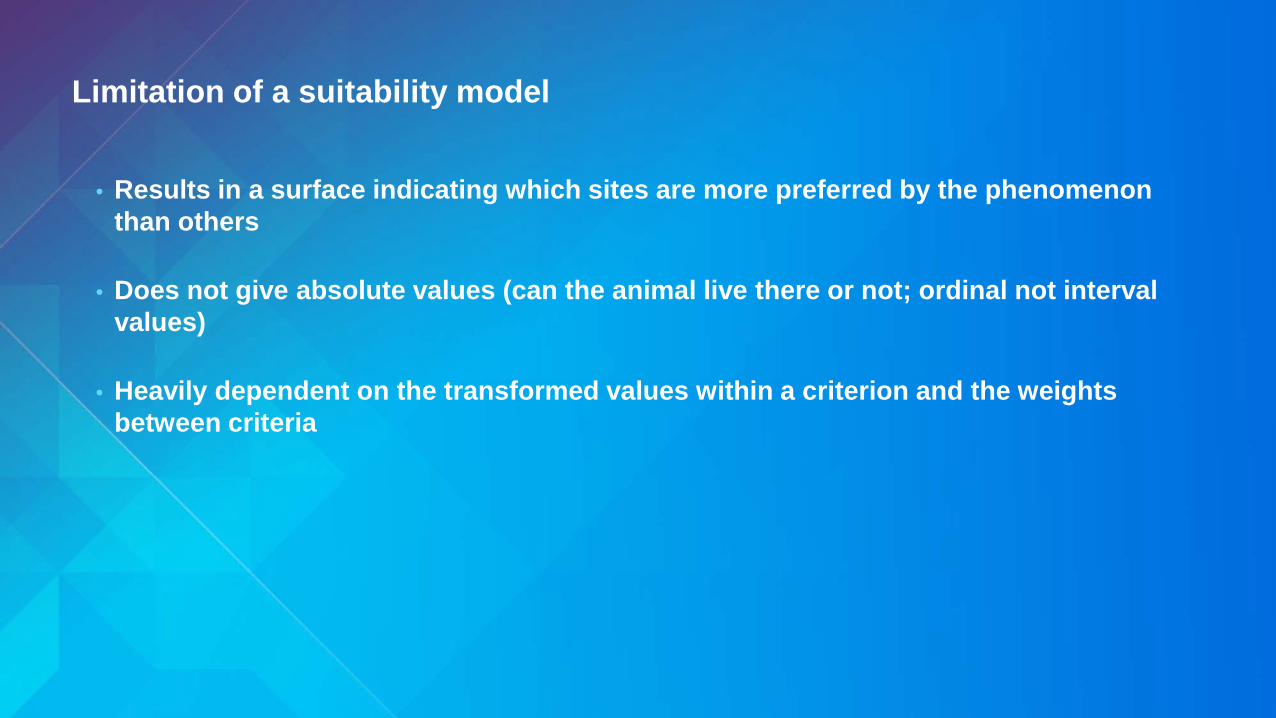
Limitation of a suitability model

• Results in a surface indicating which sites are more preferred by the phenomenon than others

• Does not give absolute values (can the animal live there or not; ordinal not interval values)

• Heavily dependent on the transformed values within a criterion and the weights between criteria

The story is not over

• How the values are transformed within criterion and weighted between criteria have not been critically examined

• Do the transformed values accurately capture the phenomenon?

• The transformation of the values was done by expert opinion – are there other approaches?

• Continuous criterion were reclassified by equal interval

• Assumes more of the good features the better

• What happens when there are many criteria?

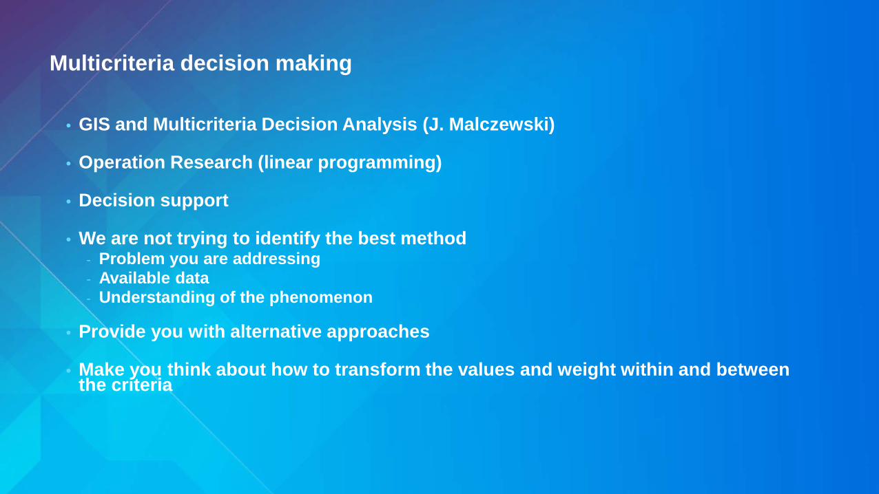
Multicriteria decision making

• GIS and Multicriteria Decision Analysis (J. Malczewski)

• Operation Research (linear programming)

• Decision support

• We are not trying to identify the best method - Problem you are addressing - Available data - Understanding of the phenomenon

• Provide you with alternative approaches

• Make you think about how to transform the values and weight within and between the criteria



Feedback

Feedback

Define the goal



Feedback

Validate results


• Objectives and criteria - Build on slopes less than 2 percent

• Many times take on the form: - Minimize cost; Maximize the visual quality

• The more the better; the less the better

• Proxy criteria - Reduce the lung disease – amount of carbon dioxide

• How to determine influence of the attributes - Literature, studies, Survey opinions - Conflicts?

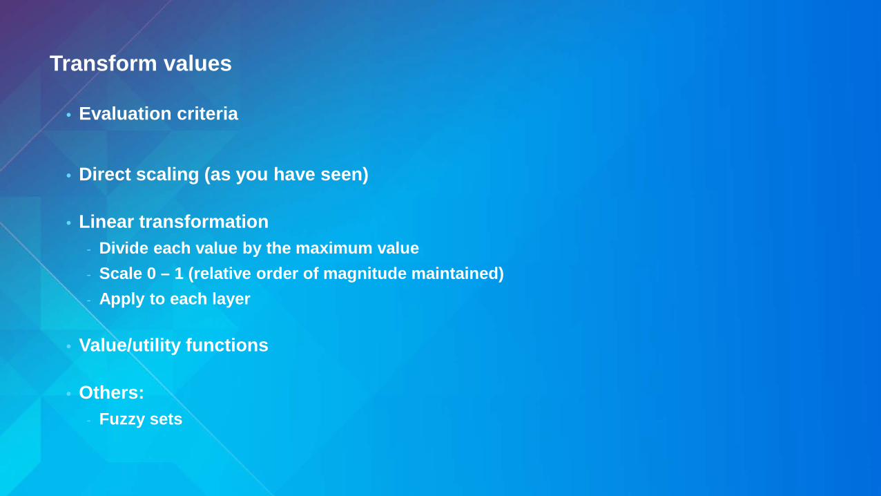
Transform values

• Evaluation criteria

• Direct scaling (as you have seen)

• Linear transformation - Divide each value by the maximum value - Scale 0 – 1 (relative order of magnitude maintained) - Apply to each layer

• Value/utility functions

• Others: - Fuzzy sets

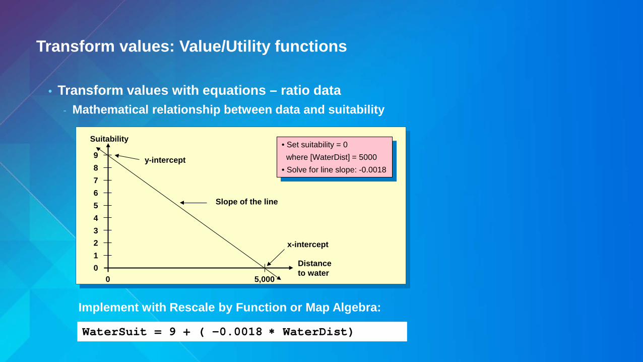
Transform values: Value/Utility functions

• Transform values with equations – ratio data - Mathematical relationship between data and suitability

• Set suitability = 0 where [WaterDist] = 5000 • Solve for line slope: -0.0018

1 2 3 4 5 6 7 8 9

0 0 5,000

Distance to water

Suitability

y-intercept

x-intercept

Slope of the line

WaterSuit = 9 + ( -0.0018 ∗ WaterDist)

Implement with Rescale by Function or Map Algebra:

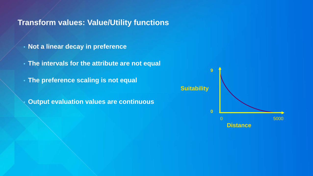
Transform values: Value/Utility functions

• Not a linear decay in preference

• The intervals for the attribute are not equal

• The preference scaling is not equal

• Output evaluation values are continuous

Distance

Suitability

9

0 0 5000

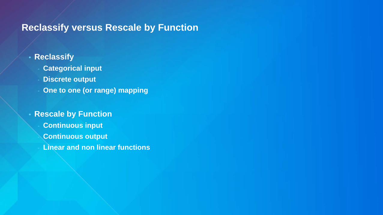
Reclassify versus Rescale by Function

• Reclassify - Categorical input - Discrete output - One to one (or range) mapping

• Rescale by Function - Continuous input - Continuous output - Linear and non linear functions

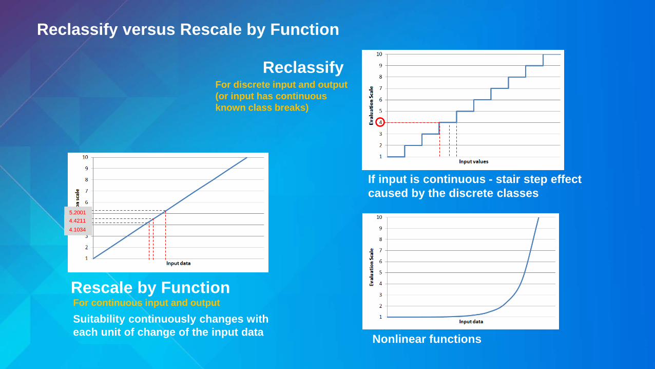
Reclassify versus Rescale by Function

Reclassify

If input is continuous - stair step effect caused by the discrete classes

Rescale by Function

4.1034 4.4211 5.2001

Suitability continuously changes with each unit of change of the input data Nonlinear functions

For continuous input and output

For discrete input and output (or input has continuous known class breaks)

Rescale by Function: the functions

Exponential

Gaussian Logistic decay

Power Large

The function can be further refined by the function parameters

Suitability workflow

Input data Derive data Transform to common Scale Final map

2 -> 1 13 -> 8 15 -> 10 21 -> 4

Reclassify

Rescale by Function

Table

Landuse

Elevation

Distance from schools

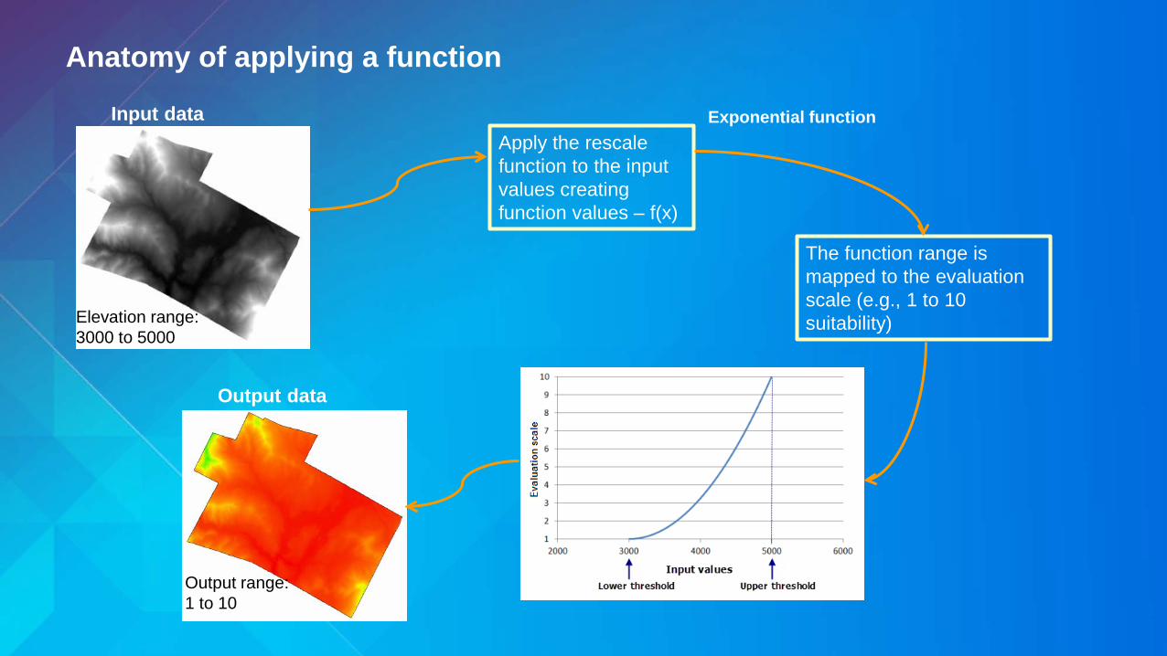
Anatomy of applying a function

Apply the rescale function to the input values creating function values – f(x)

The function range is mapped to the evaluation scale (e.g., 1 to 10 suitability) Elevation range:

3000 to 5000

Input data Exponential function

Output data

Output range: 1 to 10

Rescale by Function – Data dependent

Input range in study area: 3000 to 5000

Suitability of deer within the study area: Data dependent scenario

Suitability of deer relative to population: Data independent scenario

Suitability of deer within the study area that reach a threshold

Decision alternatives and constraints

• Constraints - Reduces the number of alternatives - Feasible and non feasible alternatives

• Types of Constraints - Non compensatory

- No trade offs - in or out (legal, cost, biological) - Compensatory

- Examines the trade offs between attributes - Pumping water – (height versus distance relative a cost)

• Decision Space - Dominated and non-dominated alternatives

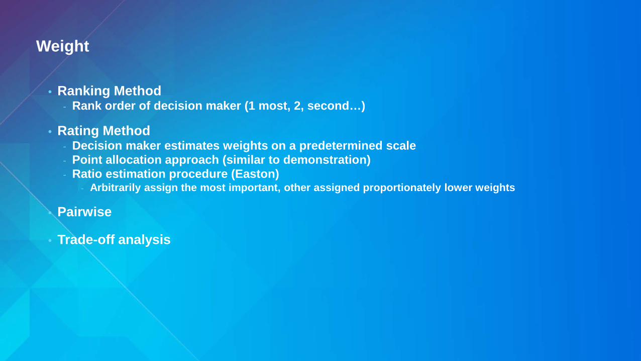
Weight

• Ranking Method - Rank order of decision maker (1 most, 2, second…)

• Rating Method - Decision maker estimates weights on a predetermined scale - Point allocation approach (similar to demonstration) - Ratio estimation procedure (Easton)

- Arbitrarily assign the most important, other assigned proportionately lower weights

• Pairwise

• Trade-off analysis

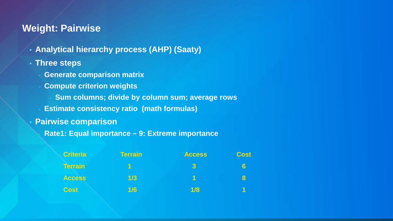
Weight: Pairwise

• Analytical hierarchy process (AHP) (Saaty) • Three steps

- Generate comparison matrix - Compute criterion weights

- Sum columns; divide by column sum; average rows - Estimate consistency ratio (math formulas)

• Pairwise comparison - Rate1: Equal importance – 9: Extreme importance

Criteria Terrain Access Cost

Terrain 1 3 6

Access 1/3 1 8

Cost 1/6 1/8 1

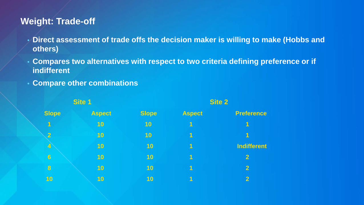
Weight: Trade-off

• Direct assessment of trade offs the decision maker is willing to make (Hobbs and others)

• Compares two alternatives with respect to two criteria defining preference or if indifferent

• Compare other combinations Site 1 Site 2 Slope Aspect Slope Aspect Preference

1 10 10 1 1

2 10 10 1 1

4 10 10 1 Indifferent

6 10 10 1 2

8 10 10 1 2

10 10 10 1 2

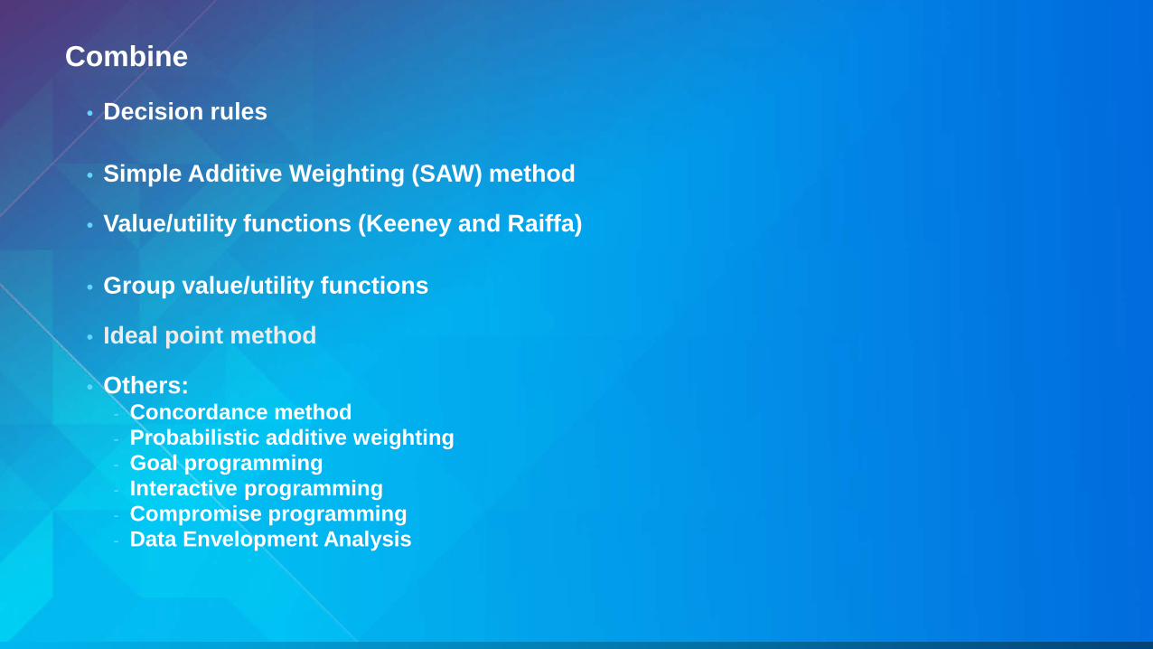
Combine

• Decision rules

• Simple Additive Weighting (SAW) method

• Value/utility functions (Keeney and Raiffa)

• Group value/utility functions

• Ideal point method

• Others: - Concordance method - Probabilistic additive weighting - Goal programming - Interactive programming - Compromise programming - Data Envelopment Analysis

Combine: SAW

• What we did earlier

• Assumptions: - Linearity - Additive

- No interaction between attributes

• Ad hoc

• Lose individual attribute relationships

• All methods make some trade offs

Combine: Group Value

• Method for combining the preferences of different interest groups • General steps:

- Group/individual create a suitability map - Individuals provide weights of influence of the other groups - Use linear algebra to solve for the weights for each individual’s output - Combine the outputs

• Better for value/utility functions

Combine: Ideal Point

• Alternatives are based on separation from the ideal point • General steps

- Create weighted suitability surface for each attribute - Determine the maximum value - Determine the minimum value - Calculate the relative closeness to the ideal point

- Rank alternatives

• Good when the attributes have dependencies

Ci+ = sj- s i+ + si-



Feedback

Feedback

Define the goal



Feedback

Validate results

Validate results: Sensitivity analysis (and error analysis)

• Systematically change one parameter slightly

• See how it affects the output

• Error - Input data - Parameters - Address by calculations or through simulations


• Background


• Demonstration


• Demonstration

• Fuzzy logic

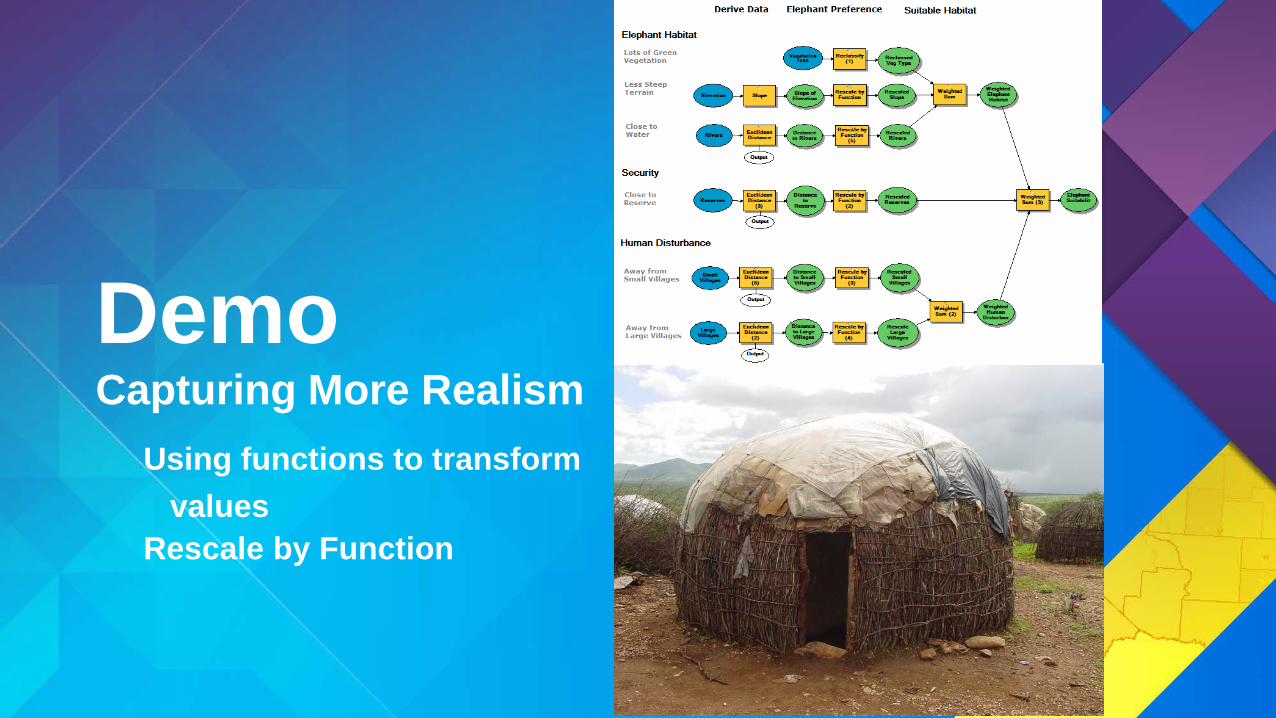
Demo Capturing More Realism Using functions to transform values Rescale by Function

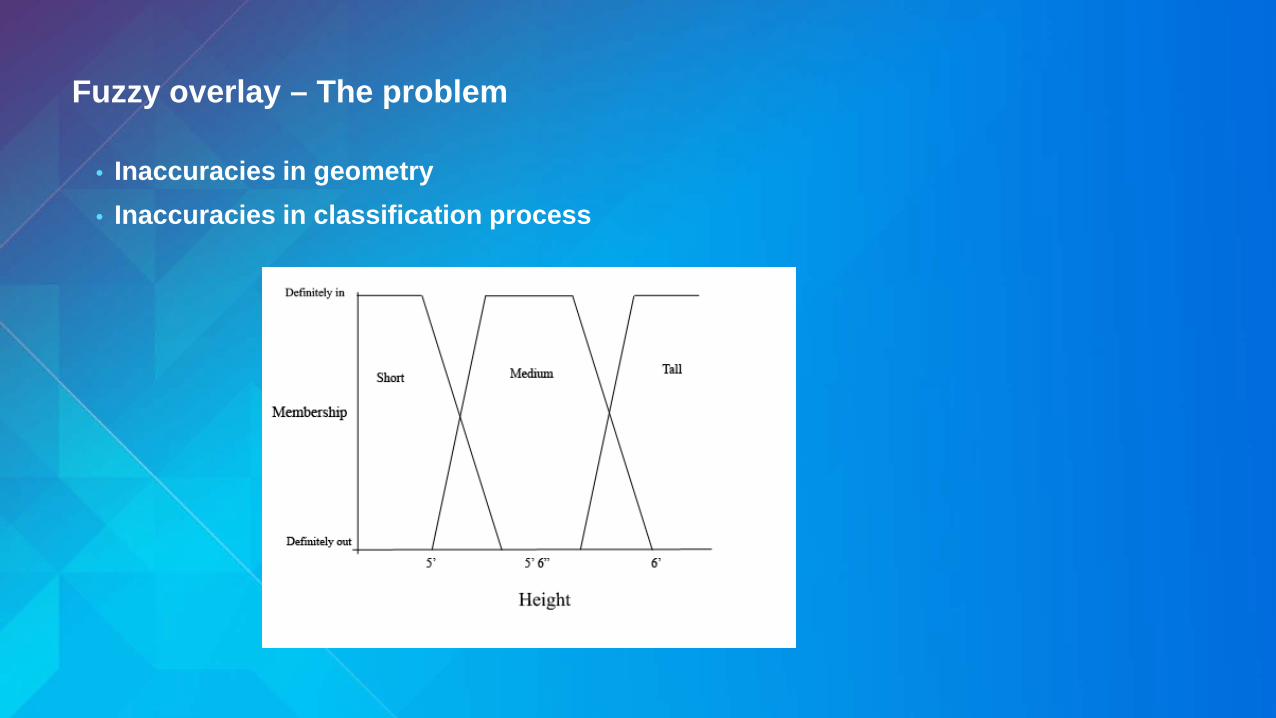
Fuzzy overlay – The problem

• Inaccuracies in geometry • Inaccuracies in classification process

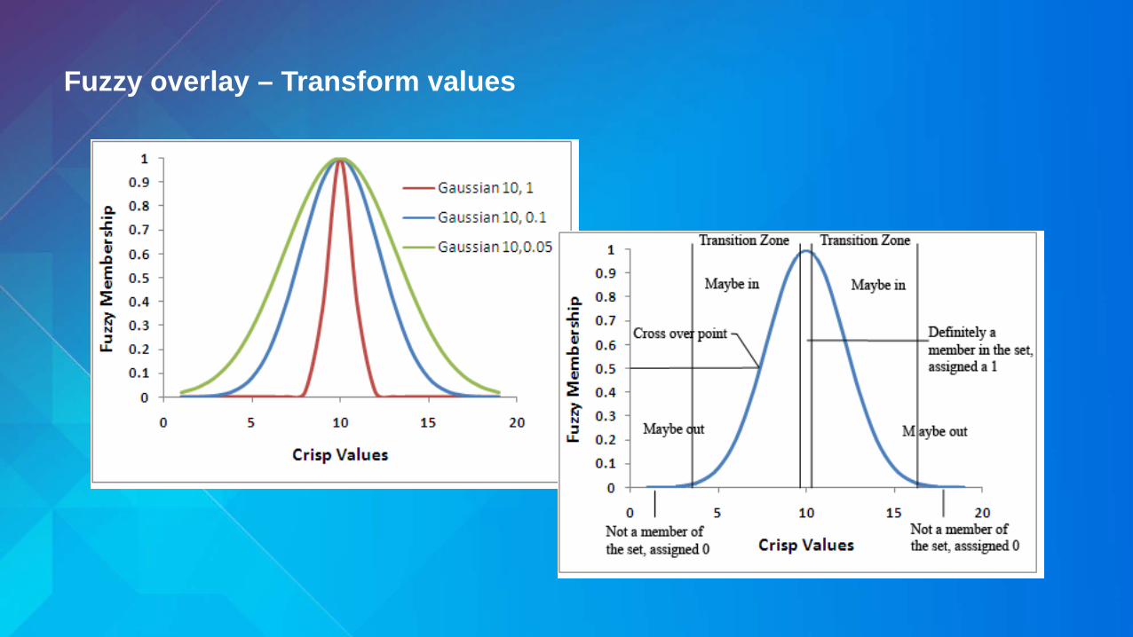
Fuzzy overlay – Transform values

• Predetermined functions are applied to continuous data

• 0 to 1 scale of possibility belonging to the specified set

• Membership functions - FuzzyGaussian – normally distributed midpoint - FuzzyLarge – membership likely for large numbers - FuzzyLinear – increase/decrease linearly - FuzzyMSLarge – very large values likely - FuzzyMSSmall - very small values likely - FuzzyNear- narrow around a midpoint - FuzzySmall – membership likely for small numbers

Fuzzy overlay – Transform values

Fuzzy overlay - Combine

• Meaning of the transformed values - possibilities therefore no weighting

• Analysis based on set theory

• Fuzzy analysis - And - minimum value - Or – maximum value - Product – values can be small - Sum – not the algebraic sum - Gamma – sum and product

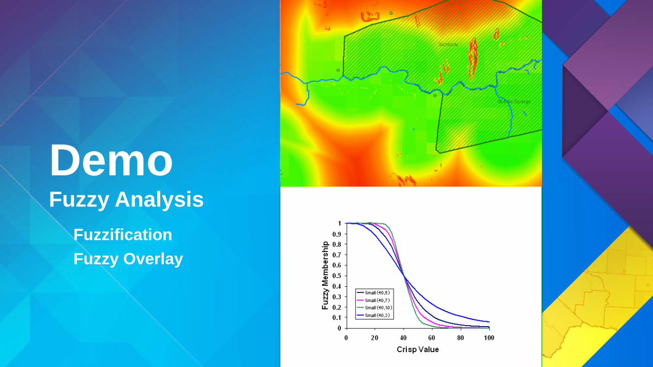
Demo Fuzzy Analysis Fuzzification Fuzzy Overlay

Summary

• Problems with: - Locate - if cells need to be contiguous - Allocating one alternative influences the suitability of another

• Can be done in the vector world • Multiple ways to transform values and define weights • Multiple ways to combine the criteria • Your transformation values and weights depend on:

- the goal - the data - the understanding of the phenomenon

• How the values are transformed and weights defined can dramatically change the results

Carefully think about how you transform your values within a criterion and weight between the criteria

spatial analyst - suitability modeling - esri...the suitability modeling model steps • determine...

Documents