spatial analysis of fatal and injury crashes in flanders ... · pirdavani, brijs, bellemans and...

Pirdavani, Brijs, Bellemans and Wets 1

Spatial Analysis of Fatal and Injury Crashes in

Flanders, Belgium; Application of

Geographically Weighted Regression Technique

Ali Pirdavani, Tom Brijs,

Tom Bellemans and Geert Wets1

Transportation Research Institute (IMOB)

Hasselt University

Wetenschapspark – Building 5

B-3590 Diepenbeek, Belgium

Tel: +32(0)11 26 91{39, 55, 27, 47, 58}

Fax: +32(0)11 26 91 99

Email: {ali.pirdavani, tom.brijs, tom.bellemans,

geert.wets}@uhasselt.be

Total number of words: 7563 (3 Tables and 3 Figures included)

Date of 1st submission: 24/07/2012

Date of 2nd

submission: 15/11/2012

1 Corresponding author

mailto:ali.pirdavani,%20tom.brijs,%20tom.bellemans,geert.wets%[email protected]

mailto:ali.pirdavani,%20tom.brijs,%20tom.bellemans,geert.wets%[email protected]


ABSTRACT 1

Generalized Linear Models (GLMs) are the most widely used models utilized in crash prediction 2 studies. These models illustrate the relationships between the dependent and explanatory 3 variables by estimating fixed global estimates. Since the crash occurrences are often spatially 4 heterogeneous and are affected by many spatial variables, the existence of spatial correlation in 5

the data is examined by means of calculating Moran’s I measures for dependent and explanatory 6 variables. The results indicate the necessity of considering the spatial correlation when 7 developing crash prediction models. The main objective of this research is to develop different 8 Zonal Crash Prediction Models (ZCPMs) within the Geographically Weighted Generalized 9 Linear Models (GWGLM) framework in order to explore the spatial variations in association 10

between Number of Injury Crashes (NOICs) (including fatal, severely and slightly injury 11

crashes) and other explanatory variables. Different exposure, network and socio-demographic 12

variables of 2200 Traffic Analysis Zones (TAZs) are considered as predictors of crashes in the 13 study area, Flanders, Belgium. To this end, an activity-based transportation model framework is 14 applied to produce exposure measurements while the network and socio-demographic variables 15 are collected from other sources. Crash data used in this study consist of recorded crashes 16

between 2004 and 2007. GWGLMs are developed using a Poisson error distribution and are 17 often referred to as Geographically Weighted Poisson Regression (GWPR) models. Moreover, 18

the performances of developed GWPR models are compared with their corresponding GLMs. 19 The results show that GWPR models outperform the GLM models; this is due to the capability of 20 GWPR models in capturing the spatial heterogeneity of crashes. 21


1. INTRODUCTION 1

For many years, researchers have attempted to investigate the negative impacts of growing travel 2 demand on traffic safety by predicting the number of crashes based on the patterns they have 3 learnt from crashes that occurred in the past. This should lead to providing a predictive tool 4 which is capable of evaluating road safety at the planning-level. Dealing with traffic safety at the 5

planning-level requires the ability to integrate Travel Demand Management (TDM) policies into 6 a crash predicting context. TDM policies are usually performed at a more aggregate level than 7 just on the level of an individual intersection or road section. Thus, the impact of adopting a 8 TDM strategy on transportation or traffic safety should be evaluated at a higher level rather than 9 merely the local consequences. Application of Crash Prediction Models (CPMs) at a macro level 10

like Traffic Analysis Zone (TAZ) leads to a type of prediction models commonly referred to as 11

Zonal Crash Prediction Models (ZCPMs). ZCPMs have been initially introduced by Levine et al. 12

based on Linear Regression models (1). However, the most common modeling framework for 13 ZCPMs is the Generalized Linear Modeling (GLM) framework (2–19). Within a GLM 14 framework, fixed coefficient estimates explain the association between the dependent variable 15 and the explanatory variables. In other words, a single model tries to fit the observed data for all 16

locations (TAZs) similarly. Expectedly, different spatial variation may be observed for different 17 explanatory variables especially where the study area is relatively large. Neglecting this spatial 18

variation may deteriorate the predictive power of ZCPMs. 19 Spatial variation is known to be an important aspect of traffic safety analysis and in 20

particularly crash prediction modeling. Inclusion of spatial variation in traffic safety studies has 21

been reported by many researchers. In one of the earliest studies, the spatial relationship between 22 activities which generate trips and motor vehicle accidents was studied and applied to the City 23

and County of Honolulu (20). Different spatial patterns for different variables such as 24 population, employment and road characteristics were identified. LaScala et al. (21) found that 25

significant spatial relationships exist between specific environmental and demographic 26 characteristics of the City and County of San Francisco and pedestrian injury crashes. Flahaut et 27

al. (22) presented different methods for identifying and delimiting accidents black-zones. This 28 was an application of spatial correlation in defining accident black-zones which share similar 29 characteristics. A similar study was carried out by Moons et al. (23) where the structure of the 30

underlying road network is taken into account by applying Moran's I to identify crash hot zones. 31 In another study by Flahaut (24), it was indicated that spatial autocorrelation should be integrated 32 in the modeling process if spatial data are being studied. He concluded that spatial models in 33 comparison to non-spatial models, do not overestimate the significance of explanatory variables; 34

thus, spatial variation should be considered to analyze spatial data. Geurts et al. (25) investigated 35 the clustering phenomenon in road accidents. This was an application of spatial analysis in traffic 36

safety that aims to analyze the characteristics of specific zones on which more accident occur. 37 Spatial correlation was found to be significant in injury crashes in a study conducted for the State 38 of Pennsylvania at the county level (9). Aguero-Valverde and Jovanis (26) further explored the 39 effect of spatial correlation in models of road crash frequency at the segment level. The results of 40 their study highlighted the importance of including spatial correlation in road crash modeling 41

studies. The models with spatial correlation show significantly better fit compared to the Poisson 42 lognormal models. The existence of clusters in the spatial arrangement of pedestrian crashes was 43 reported by (27). They supported their conclusions by computing Moran’s I value and presenting 44

the Local Indicators of Spatial Association (LISA) significance map of crashes. Huang et al. (28) 45


performed a county-level road safety analysis for the state of Florida. They reported that 1 significant spatial correlations in crash occurrence were identified across adjacent counties. 2

This spatial variation which is often referred to as “spatial non-stationarity” is overlooked 3

by the GLMs. Following such a modeling approach ends up with a set of fixed global variable 4 estimates which are the same for different TAZs; however, it is possible that an explanatory 5 variable which is found to be a significant predictor of crashes in some TAZs might not be a 6 powerful predictor in other TAZs. There are different spatial modeling techniques that have been 7 applied by many researchers in the crash prediction field. Auto-logistic models, Conditional 8

Auto-regression (CAR) models, Simultaneous Auto-regression (SAR) models, spatial error 9 models (SEM), Generalized Estimating Equation (GEE) models, Full-Bayesian Spatial models, 10 Bayesian Poisson-lognormal models are some of the most employed techniques to conduct 11 spatial modeling in traffic safety (9), (20), (24), (26), (28–34). The output of these models are 12

still fixed variable estimates for all locations, however the spatial variation is taken into account. 13 Another solution for taking the spatial variation into account is developing a set of local models, 14

so called Geographically Weighted Regression (GWR) models (35). These models rely on the 15 calibration of multiple regression models for different geographical entities. The GWR approach 16 has mainly been followed in health, economic and urban studies. Also a few studies have been 17

carried out in the transportation field using this technique (36–41). In traffic safety, Hadayeghi et 18 al. (3) developed GWR models to investigate spatial variations in the model relationships. The 19

results of the GWR models indicated an improvement in model predictability by means of an 20 increased R

2. In another study (42), bicycle crashes were studied in Buffalo, New York. Density 21

of development, physical road characteristics, socioeconomic and demographic variables were 22

the selected explanatory variables. Given the spatial nature of these variables, a GWR model was 23 developed and showed a better performance compared with the conventional model. An inter-24

province difference in traffic accidents in Turkey was studied by Erdogan (43). Different spatial 25 autocorrelation analyses were performed to see whether the accidents are clustered or not. Since 26

the results of these analyses indicated non-stationarity in the data, a GWR model was developed. 27 They also showed that the GWR model performs better than the Ordinary Least Square (OLS) 28

model. 29 The GWR technique can be adapted to GLM models and form Geographically Weighted 30

Generalized Linear Models (GWGLMs) (35). GWGLMs are able to serve the count data (such as 31 number of crashes) while simultaneously accounting for the spatial non-stationarity. Hadayeghi 32

et al. (11) used the GWR technique in conjunction with the GLM framework using the Poisson 33 error distribution. They developed different Geographically Weighted Poisson Regression 34 (GWPR) models to associate the relationship between crashes and a number of predictors. The 35 results of the comparisons between GLMs and GWPR models revealed that the GWPR models 36

outperform the GLMs since they are capable of capturing spatially dependent relationships. 37 The first objective of this paper is to examine the existence of spatial correlation in the 38

dependent and other explanatory variables available in the data. The main objective of this study 39

is then to develop different ZCPMs within the GWGLM framework in order to explore the 40 spatial variations in association between crashes and other explanatory variables. Moreover, the 41 performance of GWGLMs will be compared with the GLMs developed in an earlier study (44). 42 In this study GWGLMs are developed using a Poisson error distribution; henceforth, we refer to 43 these models as GWPR models. 44

45


2. METHODOLOGY 1

2.1. Data Preparation 2

The required information to construct the prediction models consists of exposure, network and 3 socio-demographic data accompanied with the crash data. These data should be collected for the 4 whole study area and also be aggregated to the zonal level. The study area in this research is the 5

Dutch speaking region in northern Belgium, Flanders. 6 Exposure is an important determinant of traffic safety. Therefore, it is essential to have 7

the exposure metrics as accurately as possible. To this end, the FEATHERS (Forecasting 8 Evolutionary Activity-Travel of Households and their Environmental RepercussionS) activity-9 based transportation model is applied. The FEATHERS framework (45) was developed in order 10

to facilitate the development of activity-based models for transportation demand in Flanders, 11

Belgium. The real-life representation of Flanders is embedded in an agent-based simulation 12

model which consists of over 6 million agents, each agent representing one member of the 13 Flemish population. A sequence of 26 decision trees is used in the scheduling process and 14 decisions are based on a number of attributes of the individual (e.g. age, gender), of the 15 household (e.g. number of cars) and of the geographical zone (e.g. population density, number of 16

shops). For each individual with its specific attributes, the model simulates whether an activity 17 (e.g. shopping, working, and etc.) is going to be carried out or not. Subsequently, the location, 18

transport mode and duration of the activity are determined, taking into account the attributes of 19 the individual (46). As such, the FEATHERS activity-based model can provide the exposure 20 measure by means of time-of-day dependent Origin-Destination (OD) matrices for all traffic 21

modes (i.e. Number of Trips (NOTs)). Assigning the OD matrices of car trips to the Flemish 22 road network provides other exposure variables like Vehicle Kilometers Traveled (VKT) and 23

Vehicle Hours Traveled (VHT). These network level exposure measures are then aggregated to 24 the zonal level comprising of 2200 TAZs. In addition, for each TAZ a set of socio-demographic 25

and network variables were derived. The crash data used in this study consist of a geo-coded set 26 of injury crashes (including fatal, severely injured and slightly injured crashes) that have 27

occurred during the period 2004 to 2007. Table 1 shows a list of variables, together with their 28 definition and descriptive statistics, which have been used in developing the models presented in 29 this paper. 30

2.2. Motivation for Conducting Spatial Analysis 31

Previous research has indicated that there might be significant spatial correlations in crash 32 occurrence across different locations TAZs; e.g. (11), (27), (28), (34), (43). Therefore, it is 33

essential to check for the existence of spatial correlation of dependent and explanatory variables. 34 This can be carried out by means of different statistical tests such as Moran’s autocorrelation 35 coefficient commonly referred to as Moran’s I. The results of the analysis indicate the necessity 36 of considering this spatial correlation since the spatial status of all variables are found to be non-37

stationary. 38


TABLE 1 List of Explanatory Variables for the ZCPMs with Their Definition and Descriptive 1 Statistics 2

3

4

Variable Definition Average Min Max SDa

Crash total NOICs observed in a TAZ 36.03 0 326 41.58

Exposu

re v

aria

ble

s

Number of Trips average daily number of trips originating/destined from/to a TAZ 2765.8 0 18111.4 2869.8

Total Flow Average Annual Daily Traffic (AADT) in a TAZ (vehicle) 96414.5 70.9 4423325 181695

VHT total daily vehicle hours traveled in a TAZ 608.26 1.50 9998.6 930.29

VKT total daily vehicle kilometers traveled in a TAZ 52533.8 84.06 985192 90715.2

Motorway Flow AADT of motorways in a TAZ (vehicle) 37724.96 0 3881777 146757.5

Motorway VHT total daily vehicle hours traveled on motorways in a TAZ 260.52 0 9762.5 832.97

Motorway VKT total daily vehicle kilometers traveled on motorways in a TAZ 27471.82 0 946152.8 84669.53

Other Roads Flow AADT of other roads in a TAZ (vehicle) 58690.29 0 734152.5 73632.5

Other Roads VHT total daily vehicle hours traveled on other roads in a TAZ 348.51 0 3777.69 358.76

Other Roads VKT total daily vehicle kilometers traveled on other roads in a TAZ 26662.85 0 303237.6 28133.04

V/C average volume to capacity in a TAZ 0.0478 0 0.5697 0.0422

Net

work

var

iable

s

Speed average speed limit in a TAZ (km/hr) 69.4 31 120 10.91

Capacity hourly average capacity of links in a TAZ 1790.1 1200 7348.1 554.6

Area total surface area of a TAZ in square kilometers 6.09 0.09 45.22 4.78

No. of Links number of links in a TAZ 39.27 1 230 30.46

Link Length total length of the links in a TAZ (km) 15.86 0.39 87.95 10.79

Link Density link length per square kilometers in a TAZ 3.37 0.03 20.44 2.41

Intersection total number of intersections in a TAZ 5.8 0 40 5.9

Intersection Density number of intersection per square kilometers 1.76 0 50.63 3.39

Motorway

presence of motorway in a TAZ describes as below:

“No” represented by 0

“Yes” represented by 1

0 0 1 -b

Urban

Is the TAZ in an urban area?


“Yes” represented by 1

0 0 1 -

Suburban

Is the TAZ in a suburban area?


“Yes” represented by 1 0 0 1 -

Soci

o-d

emogra

phic

var

iable

s

Driving License average driving license ownership in a TAZ describes as

percentage 81.1 0 100 3.5

Income Level

average income of residents in a TAZ describes as below:

“Monthly salary less than 2249 Euro” represented by 0

“Monthly salary more than 2250 Euro” represented by 1

1 0 1 -

Work Status

average work status of the residents in a TAZ describes as below:

“Don’t work” represented by 0

“Work” represented by 1

1 0 1 -

Population total number of inhabitants in a TAZ 2614.52 0 15803 2582.6

Population Density population per square kilometers 774.14 0 14567.4 1398.4

a: Standard deviation b: Data not applicable.


2.3. Model Construction 1

Generalized Linear Model 2

Reviewing the literature for different model forms showed that the following model has been 3

widely used in different studies (7), (14), (17), (18): 4

Where is the expected crash frequency, and are model parameters, 5

is the exposure variable (e.g. VHT, VKT or NOTs) and are the other explanatory variables. 6

Logarithmic transformation of equation (5) when considering only one exposure variable 7

yields: 8

Geographically Weighted Generalized Linear models 9

The Geographically Weighted form of Equation (6) would be: 10 11

The output of these models will be different location-specific estimates for each case 12 (here each TAZ). All variable estimates are functions of each location (here the centroid of each 13

TAZ), representing the x and y coordinates of the ith

TAZ. The main purpose of 14

developing geographically weighted models is that these models allow the estimates to vary 15 where different spatial correlation among the explanatory variables exists. If the aim is 16

estimating parameters for a model at a specific location, expectedly the locations nearby this 17 location have a greater impact on this estimation compared with the locations which are far from 18 it. This impact can be expressed by a weighting function. This weighting function is conditioned 19

on the location and changes for each location (35). The weights are derived from a weighting 20 scheme which is commonly referred to as a kernel. There are two kernels which are frequently 21 used to generate the weighting scheme; the Gaussian and the bi-square functions which can be 22 formulated as follows: 23

Gaussian function:

24

bi-square function:

25

Where represents the measure of contribution of location j when calibrating the 26

model for location i, is the distance between locations i and j and is the bandwidth (35). It is 27

reported in the literature (11), (47) that selection of the kernel function and accordingly the 28 bandwidth is very critical as the model might be very sensitive to this selection. However, 29

Fotheringham et al. (35) indicated that regarding the fit of the model, the choice of a bandwidth 30 is more important than the shape of the kernel. As a rule of thumb, when the sample locations are 31 commonly positioned across the study area, then a kernel with a fixed bandwidth is a suitable 32

choice for modeling. On the contrary, when the sample locations are clustered in the study area, 33


it is generally better to apply an adaptive kernel; i.e., having larger bandwidth where sample 1 locations are sparser and applying smaller bandwidth for denser sample locations. Adaptive 2 bandwidth will be displayed as a quantile of the number of adjacent locations (TAZs) which will 3

influence the weighting function (e.g. in Table 2 and for Model#4, the bandwidth value is 4 0.03369; this means that 3.369% of the adjacent TAZs, 74 TAZs out of 2200 TAZs, should be 5 selected to calculate the weighting function for each TAZ). 6

Despite the fact that parameters estimation depends on the weighting function, selecting 7 an appropriate bandwidth is a more crucial task. There are different approaches that can be used 8

in bandwidth selection. Cross-validation (CV) is a technique in which the optimal bandwidth size 9 is determined by minimizing the CV score which is formulated as follows: 10

Where n is the number of TAZs and is the fitted value of when the ith

case is left 11 out during the calibration process. 12

Another method to derive the bandwidth which provides a trade-off between Goodness-13

of-fit and degrees of freedom is minimizing the Akaike Information Criterion (AIC) (35). It is 14 reported by (48) that in the case of local regression, given the fact that the degrees-of-freedom 15

are likely to be small, including a small sample bias adjustment in the AIC definition is 16 recommended. This will lead to a corrected AIC often referred to as AICc. The formulations of 17

AIC and AICc are as follows: 18

and 19

Where D and K are respectively the deviance and the effective number of parameters in 20 the model with bandwidth b and n denotes the number of TAZs. 21

In this study, both the CV and AICc methods were applied to determine the most 22

appropriate bandwidth. The results reveal that in case of applying the AICc method, the optimum 23 derived bandwidths are very close to each other no matter which kernel function is used. The 24 computed bandwidths following the CV approach are slightly different than the ones derived by 25

the AICc approach. Since the model selection is based on the minimum AICc values, only the 26

bandwidths derived by the AICc approach will be used in model development. 27

Model development and spatial analysis are carried out using the 28 statistical software package R (49) and GWPR models are developed using a SAS macro (50) . 29

30

3. DISCUSSION ON MODEL RESULTS 31

3.1. Finding the Best Fitted Model 32

A common rule-of-thumb in the use of AICc is that if the difference in AICc values between two 33 models is more than 2, there is a substantial difference in the performance of the two models 34 (48). As can be seen in Table 2, Model#4 outperforms all other models by means of having the 35


minimum AICc value which is far lower than the AICc values of all other models. Model#4 is 1 fitted using an adaptive bandwidth and a Gaussian kernel function for the weighing function. It 2 can be concluded that for the given data, utilizing adaptive bandwidth and the Gaussian kernel 3

function will result in the best model fit. Therefore, this combination will be used to fit different 4 models by which we aim to compare the performance of GWPR models against GLM models. 5

TABLE 2 Comparison between GLM and GWPR Models 6

Model #1 Model #2 Model #3 Model #4

Coefficients Estimates Estimates Estimates Estimates

(Intercept) -4.141e+00 -2.886e+00 -6.32, -1.156

(-4.39,-3.64,-2.84) a

-5.215, -0.1736

(-3.26,-2.75,-1.92)

ln(Number of Trips) 4.520e-01 4.676e-01 0.1375, 0.7652

(0.37,0.48,0.59)

0.1471, 0.7665

(0.36,0.462,0.57)

ln(Motorways VKT) 7.744e-03 - -0.027, 0,0217

(-0.006,0.001,0.0098) -

ln(Other Roads VKT) 3.132e-01 - 0.1298, 0.4188

(0.21,0.25,0.303) -

ln(Motorways VHT) - 7.717e-03 - -0.0385, 0.0366

(-0.013,-0.002,0.011)

ln(Other Roads VHT) - 3.040e-01 - 0.1269, 0.4684

(0.229,0.27,0.343)

Capacity 3.894e-04 4.220e-04 -1.5e-4, 7.61e-4

(1.7e-4,3.1e-4,4.3e-4)

-8.8e-5, 7.1e-4

(2.1e-4,3.3e-4,4.4e-4)

Intersection 2.888e-02 2.844e-02 0.005, 0.052

(0.02, 0.026,0.031)

-0.0042, 0.053

(0.02,0.026,0.03)

Income level -1.071e-01 -1.056e-01 -0.526, 0.498

(-0.195,-0.072,0.01)

-0.5875, 0.5099

(-0.19,-0.064,0.023)

Urban 3.520e-01 2.287e-01 -0.137,0.783

(0.291,0.394,0.56)

-0.2487, 0.6552

(0.204,0.33,0.48)

Suburban 9.095e-02 5.712e-02 -0.102, 0.384

(0.07,0.145,0.233)

-0.1299, 0.376

(0.063,0.139,0.215)

Population 2.293e-05 2.340e-05 -5.4e-5, 9.23e-5

(9.6e-7,2.2e-5,3.7e-5)

-5.6e-5, 9.26e-5

(-2e-6,2.1e-5,3.5e-5)

Bandwidth - - 0.03371 0.03369

AICc 16918 16921 10713 10605

MSPE 489.74 482.41 238.27 234.82

PCC 0.869 0.871 0.929 0.931

a: minimum, maximum, (1st quartile, median, 3

rd quartile) of the parameter estimates.

Model #1: GLM Negative Binomial model using VKT and NOT

Model #2: GLM Negative Binomial model using VHT and 0OT

Model #3: GWPR model with adaptive bandwidth and Gaussian kernel using VKT and NOT

Model #4: GWPR model with adaptive bandwidth and Gaussian kernel using VHT and NOT

Comparable with our previous research (44) in which different GLM models were 7 developed, similar GWPR models are constructed to evaluate the benefits of accounting for the 8 spatial autocorrelation. The GWPR models and their corresponding GLM models are 9

summarized and their performances together with their goodness-of-fit measures are presented in 10


Tables 2. There are a number of measures that have been used in comparative analysis between 1 different models; e.g. AICc, MSPE and PCC (14). Comparing AICc, PCC and MSPE measures 2 in Table 2 shows that GWPR models outperform the GLM models. 3

3.2. Further Investigation on the Selected Model 4

As stated earlier, the results of the GWPR models are presented as sets of locally estimated 5

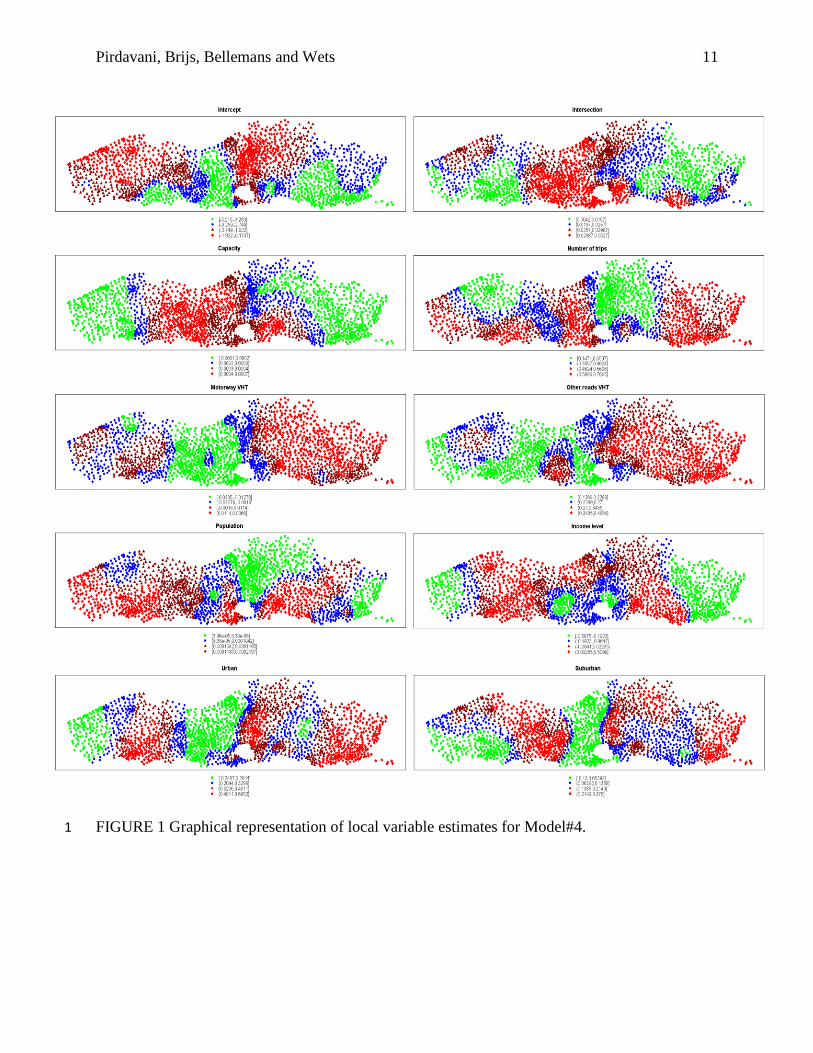
coefficients often referred to as 5-number summaries (i.e. minimum, 1st quartile, median, 3rd 6 quartile and maximum of coefficient estimates of all local models). Unlike spatially stationary 7 models (e.g. GLM models) which have a single estimate for each variable, variable estimates for 8 GWPR models vary across the space and sometimes have different and unexpected signs. Unlike 9 some other studies (11) which report on this trend to happen for their most significant variables, 10

in our study all of the most significant variables have similar signs in line with our expectations. 11 “ln(Number of Trips)” and “ln(Other Roads VHT)” as the most significant variables always have 12

positive signs for all local estimates. However the signs of other coefficients are not always the 13 same. To have a better view on these differences, local variable estimates are depicted in Figure 14 1. This issue which is often referred to as “the problem with counterintuitive signs” has already 15 been reported in many studies (11), (38), (47). One explanation for this problem would be the 16

existence of multicollinearity among some variables for some locations. It is quite possible that 17 some variables at some locations are locally correlated while no global multicollinearity 18

observed among the explanatory variables. 19 Another reason could be due to the basis of calibrating GWPR models. Presumably for 20

some locations, some variables might not be significant variables; therefore, it is possible that the 21

local models produce some unexpected variable signs for those insignificant variables. The latter 22

reason can be easily investigated by mapping local p-values. Figure 2 depicts p-values for all 23

explanatory variables of Model#4. In this figure, significant variables at any location are colored 24 in green while insignificant variables are depicted in red. By comparing Figures 1 and 2 it can be 25

concluded that the p-values for all of the locations with unexpected coefficient signs are 26 insignificant at the 95% confidence level. For instance, the variable “Urban” is expected to have 27 a positive association with the crash frequency (28), (44). As can be seen from Figure 1, only a 28

few TAZs show negative association with the NOICs (i.e. TAZs colored in green). When 29 comparing this figure with the corresponding map in Figure 2, it is evident that in these TAZs, 30

“Urban” is not a significant predictor. This is similar for other explanatory variables where the 31 TAZs with unexpected variable signs are always the TAZs where variables are insignificant 32 predictors. 33

Generally, the GWPR models outperform the GLM models because of their capability in 34

capturing spatial heterogeneity. As can be seen from Figure 3, observed and predicted NOICs are 35 having almost the same pattern. This is an indication of how well these models are able to fit the 36 observed data. 37


FIGURE 1 Graphical representation of local variable estimates for Model#4. 1


1 FIGURE 2 Graphical representations of p-values of all explanatory variables for Model#4. 2


1 FIGURE 3 Observed and predicted (results from Model#4) NOICs. 2

4. VALIDATION 3

Strong dependencies among the local coefficient estimates imply the fact that coefficients are not 4 uniquely defined and as such, any convincing interpretation cannot be derived (51). Due to the 5

greater complexities of the GWR estimation procedure that conceivably causes interrelationships 6 among the local estimates, it is essential to check for multicollinearity among local coefficient 7

estimates. There are frequently used exploratory tools available to discover possible 8 multicollinearity, such as bivariate scatter plots or bivariate correlation coefficients, however, a 9 more statistically oriented measure that adopts a simultaneous view to identify multicollinearity 10 is variance inflation factor (VIF). The VIF quantifies the severity of multicollinearity. It provides 11 an index that measures how much the variance of an estimated regression coefficient is increased 12

because of collinearity. Analyzing the magnitude of multicollinearity is carried out by 13 considering the size of the VIF. As a common rule of thumb, 10 is defined (52) as a cut off value 14 meaning that if the VIF is higher than 10 then multicollinearity is high. VIF values among local 15 coefficient estimates of models are shown in Table 3. These results suggest that multicollinearity 16

among local coefficient estimates is not a problem in any of the developed models. 17


TABLE 3 VIF Among Local Coefficient Estimates of Model#4 1

Coefficients VIF value

NOTsCars 1.550481

Motorways VHT 4.309746

Other Roads VHT 2.719767

Incomelevel 2.124447

Capacity 3.42898

Intersection 3.827387

Urban 2.347726

Suburban 1.759584

Population 2.035026

Due to the nature of GWR models which are location specific models, validation cannot 2 be accomplished by means of conventional methods (e.g. k-fold cross validation). Unlike 3

traditional regression modeling in which a general model is fitted on training dataset and 4 validated on a test dataset, GWR models are a series of local models, therefore, the concept of 5

training and testing cannot be applied in the context of GWR models. However, a new 6 framework is proposed in this research by which sensitivity of the predictability power of fitted 7 models is checked. To this end, the whole dataset is randomly divided into 10 segments. In each 8

round of model fitting one segment is left out, therefore, there will be 9 different models fitted 9

for each single data point (here TAZ). Each of these models are developed by using the derived 10 information from the neighboring TAZs. In this case, neighboring TAZs are changed in each 11 round of model fitting for each TAZ. Robustness of the prediction models can be confirmed by 12

checking the variability of predictions derived from 9 different models that are fitted for each 13 TAZ. In case of having an acceptable low variation in predictions, it could be concluded that 14

models are not sensitive to presence/absence of specific vicinity TAZs. Moreover, a low 15 variation in predictions further confirms presence of spatial correlation and the right choice of 16

bandwidth, meaning that missing information of left out TAZs are properly substituted by other 17 TAZs that have similar characteristics to the excluded TAZs. Comparing predictions of different 18

local fitted models revealed a high predictive accuracy, substantiating the robustness of models. 19

5. CONCLUSIONS AND DISCUSSION 20

Application of Generalized Linear Models (GLM) with the assumption of Negative Binomial 21 error distribution might be the most popular technique in crash prediction analysis. The results of 22 GLM models are a set of fixed coefficient estimates which represent the average relationship 23 between the dependent variable and other explanatory variables for all locations. These 24 relationships are assumed to be constant across space. However, these explanatory variables are 25

often found to be spatially heterogeneous especially when the study area is large enough to cover 26 different traffic volume, urbanization and socio-demographic patterns. In this study we first aim 27

to investigate the presence of spatial variation of dependent and different explanatory variables 28


which are being used in developing crash prediction models. This was carried out by computing 1 Moran’s I statistics for dependent and selected explanatory variables. The results revealed the 2 necessity of considering spatial correlation when developing crash prediction models. Therefore, 3

different Geographically Weighted Poisson Regression (GWPR) models were developed, using 4 different exposure, network and socio-demographic variables. GWPR models allow the 5 estimations to vary where different spatial correlation among the variables exists. Hence, the 6 association between NOICs and other explanatory variables are formed by means of different 7 local models for each TAZ. Comparing models by means of MSPE and PCC show that local 8

GWPR models always overperform global GLM models, both in fitting the data and predicting 9 the response variable. This is due to the fact that GWPR models are capable of capturing the 10 spatial heterogeneity of crash occurrence. Moreover, global estimates are unlikely to predict 11 local changes properly. For planning at local levels (e.g. municipality level), local GWR models 12

seem to be more appropriate, since global models might fail in capturing local changes. 13 Furthermore, global models’ predictions are more likely to be under/over estimated. 14

In construction of GWPR models different actions need to be taken. An important task is 15 computing the most proper bandwidth and selecting the most suitable kernel function. For the 16 current data, adaptive bandwidth with Gaussian kernel function result in the best model fit. 17

Furthermore, the AICc method is adopted to compute bandwidth. This method relies on 18 producing minimum AICc measure and has advantages compared to cross-validation (CV) 19

method. Applying the CV method might increase the risk of over-fitting the calibration data, 20 while the AICc method which penalizes possible small sample bias, accounts for the over-fitting 21 issue. 22

Another issue that needs further discussion is the choice of the Poisson error distribution 23 in this study. In traffic safety literature, utilizing the Negative Binomial error distribution is more 24

favorable than the Poisson error distribution since it accounts for overdispersion that is 25 commonly observed in crash data. However, since we accounted for spatial correlation in our 26

models, it is expect that variance will become much closer to the mean (i.e. local models are 27 fitted using a number of vicinity observation that are similar in their characteristics. This is 28

demonstrated by means of Moran’s I test for the number of crashes, indicating a significant 29 clustering pattern.). This justifies the choice of Poisson error distribution that is adopted in this 30 study. 31


REFERENCES 1

[1] N. Levine, K. E. Kim, and L. H. Nitz, “Spatial analysis of Honolulu motor vehicle crashes: I. 2 Spatial patterns,” Accident Analysis & Prevention, vol. 27, no. 5, pp. 663–674, Oct. 1995. 3

[2] E. Amoros, J. L. Martin, and B. Laumon, “Comparison of road crashes incidence and severity 4 between some French counties,” Accident Analysis & Prevention, vol. 35, no. 4, pp. 537–547, Jul. 5 2003. 6

[3] A. Hadayeghi, A. Shalaby, and B. Persaud, “Macrolevel Accident Prediction Models for Evaluating 7 Safety of Urban Transportation Systems,” Transportation Research Record: Journal of the 8 Transportation Research Board, vol. 1840, no. -1, pp. 87–95, Jan. 2003. 9

[4] R. B. Noland and L. Oh, “The effect of infrastructure and demographic change on traffic-related 10 fatalities and crashes: a case study of Illinois county-level data,” Accident Analysis & Prevention, 11 vol. 36, no. 4, pp. 525–532, Jul. 2004. 12

[5] R. B. Noland and M. A. Quddus, “A spatially disaggregate analysis of road casualties in England,” 13 Accident Analysis & Prevention, vol. 36, no. 6, pp. 973–984, Nov. 2004. 14

[6] F. L. D. De Guevara, S. Washington, and J. Oh, “Forecasting Crashes at the Planning Level: 15 Simultaneous Negative Binomial Crash Model Applied in Tucson, Arizona,” Transportation 16 Research Record: Journal of the Transportation Research Board, vol. 1897, no. -1, pp. 191–199, 17 Jan. 2004. 18

[7] G. R. Lovegrove, “Community-Based, Macro-Level Collision Prediction Models,” University of 19 British Columbia, University of British Columbia, 2005. 20

[8] A. Hadayeghi, A. S. Shalaby, B. N. Persaud, and C. Cheung, “Temporal transferability and 21 updating of zonal level accident prediction models,” Accident Analysis & Prevention, vol. 38, no. 3, 22 pp. 579–589, May 2006. 23

[9] J. Aguero-Valverde and P. P. Jovanis, “Spatial analysis of fatal and injury crashes in 24 Pennsylvania,” Accident Analysis & Prevention, vol. 38, no. 3, pp. 618–625, May 2006. 25

[10] G. R. Lovegrove and T. Sayed, “Macro-level collision prediction models for evaluating 26 neighbourhood traffic safety,” Canadian Journal of Civil Engineering, vol. 33, no. 5, pp. 609–621, 27 May 2006. 28

[11] A. Hadayeghi, A. S. Shalaby, and B. N. Persaud, “Development of planning level transportation 29 safety tools using Geographically Weighted Poisson Regression,” Accident Analysis & Prevention, 30 vol. 42, no. 2, pp. 676–688, Mar. 2010. 31

[12] G. Lovegrove and T. Sayed, “Macrolevel Collision Prediction Models to Enhance Traditional 32 Reactive Road Safety Improvement Programs,” Transportation Research Record: Journal of the 33 Transportation Research Board, vol. 2019, no. -1, pp. 65–73, Dec. 2007. 34

[13] G. R. Lovegrove and T. Litman, “Using Macro-Level Collision Prediction Models to Evaluate the 35 Road Safety Effects of Mobility Management Strategies: New Empirical Tools to Promote 36 Sustainable Development,” presented at the Transportation Research Board (TRB) 87th Annual 37 Meeting, Washington D.C. USA, 2008. 38

[14] A. Hadayeghi, “Use of Advanced Techniques to Estimate Zonal Level Safety Planning Models and 39 Examine Their Temporal Transferability,” PhD thesis, Department of Civil Engineering, University 40 of Toronto, PhD thesis, Department of Civil Engineering, University of Toronto, 2009. 41

[15] A. Naderan and J. Shahi, “Aggregate crash prediction models: Introducing crash generation 42 concept,” Accident Analysis & Prevention, vol. 42, no. 1, pp. 339–346, Jan. 2010. 43

[16] D. Lord and F. Mannering, “The statistical analysis of crash-frequency data: A review and 44 assessment of methodological alternatives,” Transportation Research Part A: Policy and Practice, 45 vol. 44, no. 5, pp. 291–305, Jun. 2010. 46

[17] M. An, C. Casper, and W. Wu, “Using Travel Demand Model and Zonal Safety Planning Model for 47 Safety Benefit Estimation in Project Evaluation,” presented at the Transportation Research Board 48 (TRB) 90th Annual Meeting, Washington D.C. USA, 2011. 49

Pirdavani, Brijs, Bellemans and Wets 17 [18] M. Abdel-Aty, C. Siddiqui, and H. Huang, “Integrating Trip and Roadway Characteristics in 1

Managing Safety at Traffic Analysis Zones,” presented at the Transportation Research Board (TRB) 2 90th Annual Meeting, Washington D.C. USA, 2011. 3

[19] A. Hadayeghi, A. Shalaby, and B. Persaud, “Safety Prediction Models: Proactive Tool for Safety 4 Evaluation in Urban Transportation Planning Applications,” Transportation Research Record: 5 Journal of the Transportation Research Board, vol. 2019, no. -1, pp. 225–236, Dec. 2007. 6

[20] N. Levine, K. E. Kim, and L. H. Nitz, “Spatial analysis of Honolulu motor vehicle crashes: II. 7 Zonal generators,” Accident Analysis & Prevention, vol. 27, no. 5, pp. 675–685, Oct. 1995. 8

[21] E. A. LaScala, D. Gerber, and P. J. Gruenewald, “Demographic and environmental correlates of 9 pedestrian injury collisions: a spatial analysis,” Accident Analysis & Prevention, vol. 32, no. 5, pp. 10 651–658, Sep. 2000. 11

[22] B. Flahaut, M. Mouchart, E. S. Martin, and I. Thomas, “The local spatial autocorrelation and the 12 kernel method for identifying black zones: A comparative approach,” Accident Analysis & 13 Prevention, vol. 35, no. 6, pp. 991–1004, Nov. 2003. 14

[23] E. Moons, T. Brijs, and G. Wets, “Identifying Hazardous Road Locations: Hot Spots versus Hot 15 Zones,” presented at the International Conference on Computational Science and Its Applications 16 (ICCSA), Perugia, Italy, 2009. 17

[24] B. Flahaut, “Impact of infrastructure and local environment on road unsafety: Logistic modeling 18 with spatial autocorrelation,” Accident Analysis & Prevention, vol. 36, no. 6, pp. 1055–1066, Nov. 19 2004. 20

[25] K. Geurts, I. Thomas, and G. Wets, “Understanding spatial concentrations of road accidents using 21 frequent item sets,” Accident Analysis & Prevention, vol. 37, no. 4, pp. 787–799, Jul. 2005. 22

[26] J. Aguero-Valverde and P. P. Jovanis, “Analysis of Road Crash Frequency with Spatial Models,” 23 Transportation Research Record: Journal of the Transportation Research Board, vol. 2061, no. -1, 24 pp. 55–63, Dec. 2008. 25

[27] C. D. Cottrill and P. (Vonu) Thakuriah, “Evaluating pedestrian crashes in areas with high low-26 income or minority populations,” Accident Analysis & Prevention, vol. 42, no. 6, pp. 1718–1728, 27 Nov. 2010. 28

[28] H. Huang, M. Abdel-Aty, and A. Darwiche, “County-Level Crash Risk Analysis in Florida,” 29 Transportation Research Record: Journal of the Transportation Research Board, vol. 2148, no. -1, 30 pp. 27–37, Dec. 2010. 31

[29] S.-P. Miaou, J. J. Song, and B. K. Mallick, “Roadway Traffic Crash Mapping: A Space-Time 32 Modeling Approach,” Journal of Transportation and Statistics, vol. 6, no. 1, pp. 33–57, 2003. 33

[30] X. Wang and M. Abdel-Aty, “Temporal and spatial analyses of rear-end crashes at signalized 34 intersections,” Accident Analysis & Prevention, vol. 38, no. 6, pp. 1137–1150, Nov. 2006. 35

[31] M. A. Quddus, “Modelling area-wide count outcomes with spatial correlation and heterogeneity: 36 An analysis of London crash data,” Accident Analysis & Prevention, vol. 40, no. 4, pp. 1486–1497, 37 Jul. 2008. 38

[32] C. Wang, M. A. Quddus, and S. G. Ison, “Impact of traffic congestion on road accidents: A spatial 39 analysis of the M25 motorway in England,” Accident Analysis & Prevention, vol. 41, no. 4, pp. 40 798–808, Jul. 2009. 41

[33] F. Guo, X. Wang, and M. Abdel-Aty, “Modeling signalized intersection safety with corridor-level 42 spatial correlations,” Accident Analysis & Prevention, vol. 42, no. 1, pp. 84–92, Jan. 2010. 43

[34] C. Siddiqui, M. Abdel-Aty, and K. Choi, “Macroscopic spatial analysis of pedestrian and bicycle 44 crashes,” Accident Analysis & Prevention, vol. 45, no. 0, pp. 382–391, Mar. 2012. 45

[35] A. S. Fotheringham, C. Brunsdon, and M. Charlton, Geographically Weighted Regression the 46 analysis of spatially varying relationships. West Sussex, England: John Wiley & Sons Ltd, 2002. 47

[36] F. Zhao and N. Park, “Using Geographically Weighted Regression Models to Estimate Annual 48 Average Daily Traffic,” Transportation Research Record: Journal of the Transportation Research 49 Board, vol. 1879, no. -1, pp. 99–107, Jan. 2004. 50

Pirdavani, Brijs, Bellemans and Wets 18 [37] A. Páez, “Exploring contextual variations in land use and transport analysis using a probit model 1

with geographical weights,” Journal of Transport Geography, vol. 14, no. 3, pp. 167–176, May 2 2006. 3

[38] L.-F. Chow, F. Zhao, X. Liu, M.-T. Li, and I. Ubaka, “Transit Ridership Model Based on 4 Geographically Weighted Regression,” Transportation Research Record: Journal of the 5 Transportation Research Board, vol. 1972, no. -1, pp. 105–114, Jan. 2006. 6

[39] H. Du and C. Mulley, “Relationship Between Transport Accessibility and Land Value: Local 7 Model Approach with Geographically Weighted Regression,” Transportation Research Record: 8 Journal of the Transportation Research Board, vol. 1977, no. -1, pp. 197–205, Jan. 2006. 9

[40] S. D. Clark, “Estimating local car ownership models,” Journal of Transport Geography, vol. 15, 10 no. 3, pp. 184–197, May 2007. 11

[41] S. Blainey, “Trip end models of local rail demand in England and Wales,” Journal of Transport 12 Geography, vol. 18, no. 1, pp. 153–165, Jan. 2010. 13

[42] E. C. Delmelle and J.-C. Thill, “Urban Bicyclists: Spatial Analysis of Adult and Youth Traffic 14 Hazard Intensity,” Transportation Research Record: Journal of the Transportation Research Board, 15 vol. 2074, no. -1, pp. 31–39, Dec. 2008. 16

[43] S. Erdogan, “Explorative spatial analysis of traffic accident statistics and road mortality among the 17 provinces of Turkey,” Journal of Safety Research, vol. 40, no. 5, pp. 341–351, Oct. 2009. 18

[44] A. Pirdavani, T. Brijs, T. Bellemans, B. Kochan, and G. Wets, “Developing Zonal Crash Prediction 19 Models with a Focus on Application of Different Exposure Measures,” Transportation Research 20 Record: Journal of the Transportation Research Board, 2012. 21

[45] D. Janssens, G. Wets, H. J. P. Timmermans, and T. A. Arentze, “Modelling Short-Term Dynamics 22 in Activity-Travel Patterns: Conceptual Framework of the Feathers Model,” presented at the 11th 23 World Conference on Transport Research, Berkeley CA, USA, 2007. 24

[46] B. Kochan, T. Bellemans, D. Janssens, and G. Wets, “Assessing the Impact of Fuel Cost on Traffic 25 Demand in Flanders Using Activity-Based Models,” presented at the Travel Demand Management 26 TDM, Vienna, Austria, 2008. 27

[47] L. Guo, Z. Ma, and L. Zhang, “Comparison of bandwidth selection in application of geographically 28 weighted regression: a case study,” Canadian Journal of Forest Research, vol. 38, no. 9, pp. 2526–29 2534, Sep. 2008. 30

[48] T. Nakaya, A. S. Fotheringham, C. Brunsdon, and M. Charlton, “Geographically weighted Poisson 31 regression for disease association mapping,” Statistics in Medicine, vol. 24, no. 17, pp. 2695–2717, 32 Sep. 2005. 33

[49] R: A language and environment for statistical computing. Vienna, Austria: R Development Core 34 Team, 2011. 35

[50] V. Y.-J. Chen and T.-C. Yang, “SAS macro programs for geographically weighted generalized 36 linear modeling with spatial point data: Applications to health research,” Computer Methods and 37 Programs in Biomedicine, vol. 107, no. 2, pp. 262–273, Aug. 2012. 38

[51] D. Wheeler and M. Tiefelsdorf, “Multicollinearity and correlation among local regression 39 coefficients in geographically weighted regression,” Journal of Geographical Systems, vol. 7, no. 2, 40 pp. 161–187, 2005. 41

[52] M. H. Kutner, C. J. Nachtsheim, and J. Neter, Applied Linear Regression Models, 4th ed. McGraw-42 Hill, 2004. 43

44

spatial analysis of fatal and injury crashes in flanders ... · pirdavani, brijs, bellemans and...

Documents