SPATIAL ACCURACY OF MEASUREMENTS USED IN CARTOGRAPHY

Vasileios C. Drosos*, Kiriaki Kitikidou* and Chrisovaladis Malesios**

vdrosos@fmenr.duth.gr, kkitikid@fmenr.duth.gr , malesios@agro.duth.gr

*Department of Forestry and Management of Environment and Natural Resources, Democritus University of Thrace, Ath. Pantazidou 193 Str.,

PC 68200, N. Orestiada, Tel.: +30 25520 41122, Fax: +30 25520 41192, **Department of Agricultural Development,

Democritus University of Thrace, Pantazidou 193, Orestiada,

Abstract: An important development in cartography has been the emergence of geometry. Besides, the word “geometry” was originally the concept of “measuring the earth”. The first examples of maps that appear to be constructed using certain principles of geometry were from Babylon. However, based on our knowledge to date, the ancient Greeks, and even the Ionians, were those given for the first time a scientific background in cartography, combining amazing knowledge with technology, theory with practice. The ancient Greeks and Romans built, made simple surveying instruments for various technical works. Station was the construction of the first theodolite by the English Engineer Sisson in 1700. With the appearance of new technologies and instruments and the contribution and development of the personal computers new perspectives are being opened and new possibilities are being created such as the Total Stations. With the conquest of space we had in the use of satellites to map the earth the well known GPS that then evolve. Finally, for greater accuracy in our time we have gone by the analog to digital maps. In this paper, investigated and shown the achieved spatial accuracy of the measurements used to create maps with the classical topographical way of data collection. The measurements were accomplished in different time of the year and under different forest conditions. To the statistic analysis the values of the total station were taken as true values. The technique is based on the original estimated accuracy and at the principal of errors transmission, to determine a number of control points. The control points distributed at random in order to achieve unbiased assessment. An accurate and reliable digital map can be a useful tool in many fields of forestry such as in forest management planning, forest protection, forest utilization, forest policy, economy, management, soil erosion, natural hazards and watershed management, cultural landscape-planning, management and protection, sustainable design in landscape planning, integral protection of forest ecosystems and urban green surfaces etc. Finally the measurements accuracy was calculated, the suitable results were drawn and the relative suggestions for the forest application are indicated Key words: mean square error, spatial accuracy, standard deviation

191

1. Introduction An important development in cartography has been the emergence of geometry. Besides, the word “geometry” was originally the concept of “measuring the earth”. The first examples of maps that appear to be constructed using certain principles of geometry were from Babylon. However, based on our knowledge to date, the ancient Greeks, and even the Ionians, were those given for the first time a scientific background in cartography, combining amazing knowledge with technology, theory with practice. The Hipparchus (190-124 BC) invented a method of location by latitude and longitude. Of course this had first to divide the globe into 360 meridians and 180 parallels. Later, the student of Aristotle Dikearchos creates his first world map by taking into account its sphericity. The mapping concerned several of the ancient Greeks, but as the prime meridian for their measurements they did not used the Greenwich one, but the meridian that runs from the Giza of Egypt and the Great Pyramid. This is the meridian which covers the majority of land of our planet. It is also the only meridian that divides land and sea in two halves! Some ancient maps have survived so far and impressed not only with the precision of their design, but mainly with the unthinkable at the time comments! Some of these have the Antarctic without ice, while others show almost picture from space. The ancient Greeks and Romans built, made simple surveying instruments for various technical works. Station was the construction of the first theodolite by the English Engineer Sisson in 1700. With the appearance of new technologies and instruments and the contribution and development of the personal computers new perspectives are being opened and new possibilities are being created such as the Total Stations. With the conquest of space we had in the use of satellites to map the earth the well known GPS that then evolve. Finally, for greater accuracy in our time we have gone by the analog to digital maps. The drawing up sector of digital maps rapidly is being evolving due to rapid technological change and the expansion of categories of customers who need maps to new forms. The maps have exceeded the original limits of their use for military and cadastral applications and wanted a growing daily basis by agencies, advertising companies and individuals. The information was so far available in analogue format maps converted to geographic data bases, in order to produce digital maps. The conventional maps are increasingly stored and updated in digital form and distributed through networks like the Internet. New applications, which use specialized digital maps are developed, such as databases on road navigation, mobile telephone etc. Most studies on current and future needs of digital map production focus on areas of writing, correction and updating databases. Particular emphasis on databases vehicle navigation, surveying and digital maps used by the telecommunications industry to design their networks and are particularly active areas of contemporary market. The use of satellite data in digital cartography is not confined to the initial draw up of maps (Figure 1). The large volume of details that are stored in databases and dynamically developed through the annual changes in the medium term raises the question of updating as the most critical.

192

In today's era of digital cartography, where the speed in creating maps, in the modification, in representation and in their final production is surprisingly large (Burrough, 1986; Dermanis, 1992), in the era of the development of hardware and software (H / W, S / W) enable high quality printing products of cartography at this time there is still a perception that the visual quality, it is also essential / measuring quality.

Figure 1. Three-dimensional remote sensing image of Sithonia peninsula the second leg of Halkidiki prefecture Many times a derivative mapping product gives the impression of quality although behind the visual effect hidden inaccurate data, errors and discord with the reality (Burrough, 1986; Boutoura, 1994). Positional accuracy is often expressed in two components: absolute and relative positional accuracy (Stanislawski et al., 1996). Absolute positional accuracy addresses how closely all the positions on a map or data layer match corresponding positions of the features they represent on the ground in a desired map projection system (Stanislawski et al., 1996). The relative positional accuracy of a map considers how closely all the positions on a map or data layer represent their corresponding geometrical relationships on the ground. Although absolute positional accuracy can be important and may also have a direct influence on the relative positional accuracy within a DIMB, only the latter is discussed in this paper. A number of standards have been developed to provide for positional assessment of cartographic maps (Merchant, 1982; Vonderohe and Chrisman, 1985; Merchant, 1987; Crosilla and Pillirone, 1995). A variation to the ASPRs standards are provided in Acharya and Bell (1992) and Ackermann and Rad (1996). Skidmore and Turner (1992) proposed a line intersect sampling technique which is directed at assessing land-cover class boundaries

193

on cartographic land-cover maps. In 1998 the Subcommittee for Base Cartographic Data, Federal Geographic Data Committee published a National Standard for Spatial Data Accuracy (NSSDA). In 1999 a technique for spatial sampling and error reporting for image map bases has been developed by Chong. In this paper, investigated and shown the achieved spatial accuracy of the measurements used to create maps with the classical topographical way of data collection. 2. Materials and methods 2.1. Research area The research area was nearby the city of Thessaloniki and in the middle of the peninsula of Kassandra, the first leg of the Halkidiki prefecture, lies between the geographic coordinates: - South end: Latitude 39 54 ́30΄ ,́ longitude 23 45 ́10΄΄. - North end: Latitude 40 18 ́20΄ ,́ longitude 23 20 ́15΄΄. The research area is called Kalandra an area with great tourist development and demand and unique beauty. Kalandra is a small town on Kassandra, the westernmost peninsula of Chalcidice. In ancient Greece it was the site of the town of Mende, one of the many colonies in Chalkidiki founded by Chalcis, the main city on the island of Euboea. Mende was also the birthplace of the sculptor Paeionius, (also Paionios), who made a statue of Nike, which was put on top of the victory pillar in Olympia, and is currently in the Archaeological Museum of Olympia. There was also a temple of Poseidon (Figure 2).

Figure 2. Research area 2.2. Instruments choice The used instruments were the LEICA VIVA GS15 and total station LEICA TC805 (Figures 3 and 4).

194

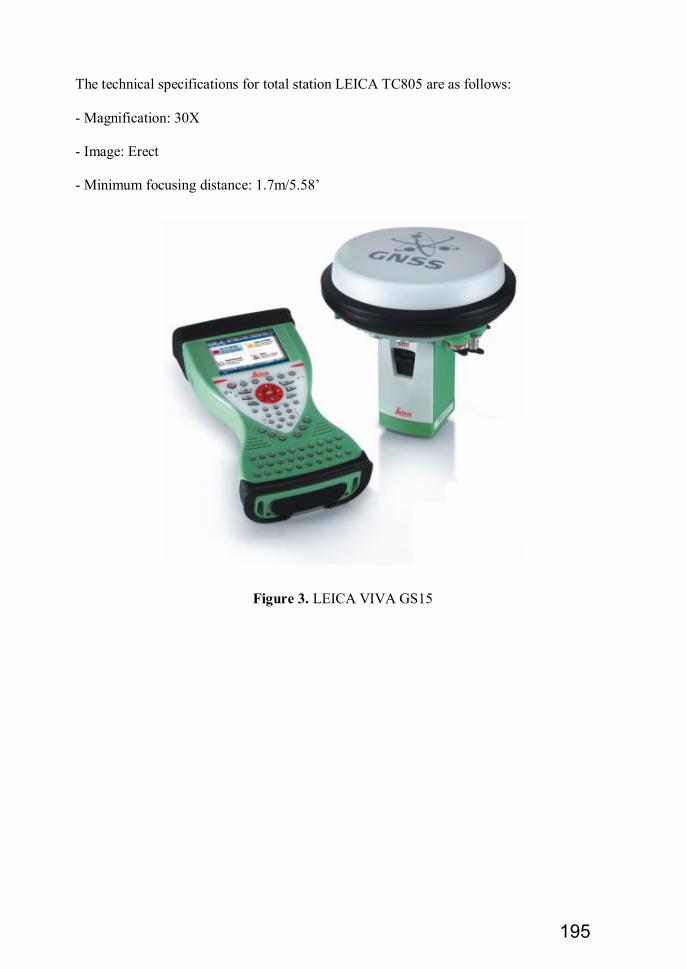
The technical specifications for total station LEICA TC805 are as follows: - Magnification: 30X - Image: Erect - Minimum focusing distance: 1.7m/5.58’

Figure 3. LEICA VIVA GS15

195

Figure 4. Total station LEICA TC805 - Angle accuracy: 5”/2mgon - Angle minimum display reading: 1” - Angle detecting system: Dual-side reading - Angle/Dist. units: Switchable between degrees, mil or gon, meter or feet, US/ft-International - Distance measurement: 1 Prism: 7,200’, 3 Prism: 24,600’, Long range: 33,000’ - Distance measurement prismless mode: 984' - Distance measurement precision: ±(3mm+2ppm) - Distance measuring time: 3s+every 0.3s tracking mode - Distance measuring time: 1s+every 0.5s coarse mode - Distance minimum display: 1mm/0.003ft - Display: Single - Internal memory: Stores 10,000 data blocks or 16,000 fixpoints - Data input/output: RS-232C

196

- Compensator: Oil dual axis - Compensating range/Accuracy: ±4’/2” - Weight: 4.2kg including tribrach and battery. The basic technical specifications of the dual frequency satellite positioning system are shown in table 1. Table 1. Basic technical specifications of satellite positioning system LEICA VIVA GS15. System Differential GPS Corrections 1.0 The GPS system consisting of two receivers interchangeable between each other

with supporting accessories, software to perform all the required applications. Receiver GPS GNSS 2.0 Have receivers of four (4) frequencies for both GPS and GLONASS satellites on.

Also be able to receive signals from the third frequency GPS L5 and GALILEO satellites and the new L2C frequency for better and faster fix.

2.1 Each receiver offers 120 channels and two frequencies L1 and L2 on simultaneous detection of up to 60 satellites at both frequencies. The receiver performs measurements of phase and frequency waves two carriers L1 and L2 code measurements and C / A and P in L1 and L2 frequencies. Each receiver has: • Sixteen (16) channels of continuous detection of the frequency of L1. • Sixteen (16) channels of continuous detection of the frequency of L2. • Sixteen (16) channels of continuous detection of the frequency of L1 GLONASS and sixteen (16) channels of continuous detection of the frequency of L2 GLONASS + (4) SBAS (WAAS, EGNOS, GAGAN, MSAS)

2.2 Ability to record observations in kinematic and static procedure for post-editing in the office.

2.3 The rate of measurements’ recording to qualify by 0.05 sec to 300 sec. The angle of the satellite measurements for recordings (cut - off angle) to be eligible.

2.4 The refresh rate of the position to be eligible by 0.05sec (20 Hz) to 1 sec (1Hz). 2.5 The system offers complete reference design parameters (availability of satellites,

static figures Precision PDOP, GDOP, and azimuth angles of the satellites, sky map) all the data is tabular and graphical format.

2.6 Has built-in anti-jam mining on both frequencies L1 and L2. 2.7 Have reliable technology of reception under trees. 2.8 The mobile receiver to receive network RTK corrections and supports networked

RTCM messages type of issue until v3.1. 2.9 The receiver is controlled via the serial port to any other program that runs on any

platform. 2.10 The data from both receivers are recorded in CF Compact Flash or SD cards in both

the receiver and the keyboard with selectable by the user to register. 2.11 The ISDN cards have at least 1GB of memory 2.12 The mobile receiver (rover) communicates with Bluetooth built-in antenna for

kinematic and REAL TIME applications. 2.13 The rover receiver (mobile) consists of the antenna, keyboard, batteries and pole

197

with the support and its weight is not more than 3.5Kg. 2.14 The operating temperature range of the receiver is-30° C.-65° C. 2.15 The storage temperature range of the receiver is -40° C. 2.16 The resistance to humidity is 100% (total precipitation). 2.19 The RTK is fully integrated in receivers. 2.20 The integrated software of the receiver allows and the following measurements:

• Surveying • Identification of reference systems • Mapping of all methods of orientation (north, sun, point, line, arrow navigation) • COGO applications for determining coordinate points with many geometric methods. Specifically: cuts straight to the field in straight distance calculations, arrows, shift, speed tracks, routes • Transformation etc. The user has the ability to create its own set of rules for all applications supported by the system and planning at the office before the field measurements.

2.21 The software has the ability to create lines and polygons as well as the possibility of introducing coding points, lines and polygons.

2.3. Accuracy control To determine whether the mean m1 of the values X1, X2, ..., Xn (measured by Leica) a sample size n (n = 37) differs significantly from the average price m2 Y1, Y2, ..., Yn (Total Station measurements) another, dependent sample size n, we calculate the quantity t as follows:

1 2

Dt s

n

where sD is the standard deviation of the variable D which is derived as follows: If a sample has values X1, X2, ..., Xn (measured by Leica) and the other Y1, Y2, ..., Yn (measured by Total Station), the variable D values are differences (X1-Y1), (X2-Y2), ..., (Xn-Yn).

1

1

n

ii

D

D Ds

n

The nil hypothesis is: H0: m1 = m2 and its alternative is: H1: m1 ≠ m2.

198

3. Results and discussion Traditionally, spatial data producers use data specifications and summary statistics to report data quality information, while the onus of applying this quality information to account for spatial uncertainty has rested with the spatial data user. Differences exist between ground measurements and their digital portrayal in geospatial data sets. There is general agreement that these differences must be described and reported along with the data, so that users can make informed decisions on the fitness of the data for specific applications (Burrough et al., 1996). Accuracy reporting typically consists of summary statistics derived from ground measurements, Total Station measurements in our case. For a digital elevation model, the statistic might be a root mean square error (RMSE) for a set of locations at which the true elevation is known, or an inference test such as t-test for normally distributed mean differences (American Society of Civil Engineers, 1983; American Society of Photogrammetry, 1985; Shearer, 1990; Goodchild, 1991). Government agencies engaged in spatial data production subject their data to accuracy assessments, typically disqualifying any that fail to meet quality specifications and reporting summary information from the assessments. These reports summarize the quality of the data as it relates to some predefined specification. As an example, consider a USGS level 2 digital elevation model (DEM). An approved DEM file must have an RMSE of less than one-half of the source interval, with no error exceeding one interval (USGS, 1995). With regard to these reports, then, producers are primarily concerned that their data meets a measure of accuracy. Regarding to our data, all RMSE’s are less than one-half of the source interval (Table 2), with only a few errors exceeding one source interval (these errors are highlighted in Table 3). Table 2. RMSE’s and source intervals for E, N and H. E N H RMSE’s 15.915 16.901 0.872 Source interval 95.9278 100.063 5.289845

199

Table 3. Errors for each sample point (n = 37). Error = │Total Station measurement – Leica measurement│ Sample point ID E N H 1 0.037 0.004 0.073 2 0.028 0.055 0.031 3 0.028 0.035 0.055 4 0.048 0.049 0.064 5 0.002 0.028 0.056 6 0.056 0.053 0.096 7 95.930 23.536 0.086 8 0.025 0.073 0.091 9 0.080 0.046 0.068 10 0.037 0.036 0.014 11 0.043 0.060 0.064 12 0.048 0.063 0.072 13 0.094 0.012 0.055 14 0.102 0.032 0.035 15 0.093 0.037 0.081 16 0.105 0.003 0.044 17 0.125 0.054 0.035 18 0.090 0.027 0.067 19 0.065 0.042 0.062 20 0.080 0.015 0.061 21 0.043 0.008 0.041 22 0.037 0.030 0.058 23 0.071 0.053 0.093 24 0.014 0.048 0.082 25 0.055 0.103 0.084 26 0.021 100.066 0.056 27 0.008 0.041 0.030 28 0.047 0.043 0.053 29 0.031 0.026 0.043 30 0.024 0.005 0.001 31 0.028 0.017 0.008 32 0.064 0.024 0.013 33 0.049 0.004 0.025 34 0.024 0.017 0.004 35 0.048 0.018 0.037 36 13.019 1.449 5.291 37 0.036 0.007 0.034

200

Assuming normally distributed mean differences for E, N and H (Kolmogorov-Smirnov test p-values were >0.05 for all paired variables), t-test showed that Leica and Total Station measurements do not have statistically important differences (p>0.05) (Table 4). Table 4. Paired variables (Total Station measurement – Leica measurement) t-test.

Pair variable Mean Std.

Deviation

Std. Error Mean

95% Confidence Interval of the

Difference t df p

Lower Upper E 2.19688 15.98049 2.62718 -3.13129 7.52504 .836 36 .409 N 3.39916 16.78441 2.75934 -2.19704 8.99536 1.232 36 .226 H -.09352 .87856 .14444 -.38645 .19941 -.647 36 .521

We observe from table 4 that generally altitudes have lower error than the error of planimetric coordinates. Also observe using the root mean square error of measurements characterizes the accuracy that the error in E (X, east) is smaller than in N (Y, north). 4. Conclusions This paper has as purpose the investigation and presentation in brief the achieved spatial accuracy of the measurements used to create maps with the classical topographical way of data collection. The proposed detection of accuracy is statistically sound and easily followed. No complicated algorithms or difficult calculations are involved. Generally, digital backgrounds and high-quality maps do not require an accurate estimate of position, because the automation in digital photogrammetric processes from which derived ensures high quality products. However, any digital map that comes from an unknown or suspicious source requires an independent and thorough evaluation. The field checks are laborious and expensive, but offer a unique precision used as a bench-mark. The recent introduction of sophisticated techniques GPS measurements in real time can provide an effective and economical technique for identification and exact location of discrete objects, hedges, shrubs and trees, an element present in abundance in digital maps. The procedure used in practice seems to be economical, it gives good results in terms of performance moves is good. The geographic data bases are a product of the cartographic interface with alphanumeric databases. Through appropriate links the digital cartographic base interactively interfacing with a database allowing user to submit, in an environment of GIS, questions of spatial form (through cartographic base) or thematic form (via the database). The quality of information is investigated, examined always with ground control. Based on the things mentioned above cannot accept that the main part of a digital map is a database of geographic data which, however, has added a mandatory set of “mapping” features, which presented not only in quality control database and the one that ensures accuracy, precision and reliability of an analog map. However, modern forestry reality in

201

Greece teaches us that more affordable and reliable tool in many cases is the map (analog model) both in terms of cost, knowledge and from the beards difficulties. An accurate and reliable digital map can be a useful tool in many fields of forestry such as in forest management planning, forest protection, forest utilization, forest policy, economy, management, soil erosion, natural hazards and watershed management, cultural landscape-planning, management and protection, sustainable design in landscape planning, integral protection of forest ecosystems and urban green surfaces etc. References Acharya, B. and Bell, W. (1992), Universal accuracy standards for GIS, Proceedings of

ASPRS/ACSM/RT 92, Washington, D.C., 3: 368-379. Ackermann, R. J. and Rad, A. (1996), Quality control procedure for photogrammetry

digital map, International Archives of Photogrammetry and Remote Sensing, 31 (B4): 12-17.

American Society of Civil Engineers (Committee on Cartographic Surveying, Surveying

and Mapping Division). (1983), Map uses, scales and accuracies for engineering and associated purposes. American Society of Civil Engineers, New York.

American Society of Photogrammetry (Committee for Specifications and Standards,

Professional Practice Division). (1985), Accuracy specification for large-scale line maps. Photogrammetric Engineering and Remote Sensing 51: 195-199.

Boutoura, H. (1994), Accuracy of primary and secondary charter with geometric content,

Two-day Conference TEE, Digital Cartography, Photogrammetry, Remote Sensing, technology, Athens, p. 53-60.

Burrough, P. A., 1986. Principles of Geographical Information Systems. Oxford University

Press. UK. Burrough, P., van Rijn, R., Rikken, M. (1996), Spatial data quality and error analysis

issues: GIS functions and environmental modeling. In Goodchild, M. et al., Eds., GIS and Environmental Modeling: Progress and Research Issues. GIS World Books, Fort Collins, CO, pp. 29-34.

Chong, A. K. (1999), A Technique for Spatial Sampling and Error Reporting for Image

Map Bases, Photogrammetric Engineering & Remote Sensing, Vol. 65, No. 10, October 1999, pp. 1195-1198.

Crosilla, P. and Pillirone, G. (1995), Parametric and non-parametric procedure for testing

the metric quality of a digital map, Manuscripts Geodaetica, 20: 231-240. Dermanis, A. (1992), Technique are indicated Observation and Theory Assessment,

Volumes I and II, Ziti Press, Thessaloniki, p. 125.

202

Federal Geographic Data Committee. (1998), National Standard for Spatial Data Accuracy (NSSDA), FGDC-STD-007.3-1998. Federal Geographic Data Committee, Washington, D. C., 25 p., (http://fgdc.er.usgs.gov/fgdc.html).

Goodchild, M. (1991), Issues of quality and uncertainty. In Muller, J., Ed., Advances in

cartography, Elsevier Applied Science, London, p. 113-139. Merchant, D. C. (1982), Spatial accuracy standards for large scale maps, Proccedings

ACSM 42nd Annual Meeting, p. 222-231. Merchant, D. C. (1987), Spatial accuracy specification for large scale topographic maps,

Photogrammetric Engineering & Remote Sensing, 53(7): 958-961. Shearer, J. (1990), Accuracy of digital terrain models, In Petrie, G, Kennie, T., Eds.,

Terrain Modelling in Surveying and Civil Engineering, Thomas Telford, London, p. 315-336.

Skidmore, A. and Turner, B. (1992), Map accuracy assessment using lines intersect

sampling, Photogrammetric Engineering & Remote Sensing, 58(10): 1453-1457. Stanislawski, L., Dewitt, B. and Shrestha, R. (1996), Estimating Positional Accuracy of

Data Layers within a GIS through Error Propagation, Photogrammetric Engineering & Remote Sensing, 62 (4): 429-433.

Vonderohe, A.P. and Chrisman, N.R. (1985), Test to establish the quality of digital

cartographic data: Some examples from the Dane Country Land Records Project, Proceedings AUTO-CARTO 7, p. 552-559.

USGS. (1995), National Mapping Program Technical Instructions. Standards for Digital

Elevation Models, U.S. Dept. Interior.

203