sparse matrix methods in - web.stanford.eduweb.stanford.edu/group/sol/papers/gmsw84.pdf · sparse...

SIAM J. ScI. STAT. COMPUT.Vol. 5, No. 3, September 1984

1984 Society for Industrial and Applied Mathematics005

SPARSE MATRIX METHODS IN OPTIMIZATION*

PHILIP E. GILL?, WALTER MURRAY’S, MICHAEL A. SAUNDERS?AND MARGARET H. WRIGHT?

Abstract. Optimization algorithms typically require the solution of many systems of linear equationsBkyk b,. When large numbers of variables or constraints are present, these linear systems could accountfor much of the total computation time.

Both direct and iterative equation solvers are needed in practice. Unfortunately, most of the off-the-shelfsolvers are designed for single systems, whereas optimization problems give rise to hundreds or thousandsof systems. To avoid refactorization, or to speed the convergence of an iterative method, it is essential tonote that B is related to Bk_ 1.

We review various sparse matrices that arise in optimization, and discuss compromises that are currentlybeing made in dealing with them. Since significant advances continue to be made with single-system solvers,we give special attention to methods that allow such solvers to be used repeatedly on a sequence of modifiedsystems (e.g., the product-form update; use of the Schur complement). The speed of factorizing a matrixthen becomes relatively less important than the efficiency of subsequent solves with very many right-handsides.

At the same time, we hope that future improvements to linear-equation software will be oriented morespecifically to the case of related matrices Bk.

Key words, large-scale nonlinear optimization, sparse matrices, sparse linear and nonlinear constraints,linear and quadratic programming, updating matrix factorizations

1. Introduction.1.1. Background. The major application of sparse matrix techniques in optimiz-

ation up to the present has been in the implementation of the simplex method forlinear programming (LP) (see, e.g., Dantzig (1963)). In fact, commercial codes forlarge LP problems seem to have predated codes for sparse linear equations (eventhough solving a sparse LP problem requires solving many sparse linear systems). Inthe commercial world today, more sparse matrix computation is probably expendedon linear programs than on any other type of problem, and linear programs involvingthousands of unknowns can be solved routinely. Because of the great success of thesimplex algorithm and the wide availability of LP codes, many large-scale optimizationproblems tend to be formulated as purely linear programs. However, we shall see thatthis limitation is often unnecessary.

Before considering particular methods, we emphasize that methods for large-scaleoptimization have a special character attributable in large part to the critical importanceof linear algebraic procedures. Since dense linear algebraic techniques tend to becomeunreasonably expensive as the problem dimension increases, it is usually necessary tocompromise what seems to be an "ideal" strategy. (In fact, an approach that wouldnot even be considered for small problems may turn out to be the best choice forsome large problems.) Furthermore, the relative cost of the steps of many optimizationmethods changes when the problem becomes large. For example, the performance of

* Received by the editors December 22, 1982, and in final form August 22, 1983. This research was

supported by the U.S. Department of Energy under contract DE-AM03-76SF000326, PA no. DE-AT03-76ER72018, the National Science Foundation under grants MCS-7926009 and ECS-8012974; the Officeof Naval Research under contract N00014-75-C-0267; and the U.S. Army Research Office under contractDAAG29-81-K-0156.

" Systems Optimization Laboratory, Department of Operations Research, Stanford University, Stanford,California 94305.

562

SPARSE MATRIX METHODS IN OPTIMIZATION 563

unconstrained optimization algorithms is often measured by the number of evaluationsof the objective function required for convergence. Although simplistic, this is areasonable gauge of effectiveness for most problems of low dimension because thenumber of arithmetic operations per iteration tends to be small, and the amount ofwork required for storage manipulation is negligible. However, as the size of theproblem grows, the "housekeeping" (cost of arithmetic and data structures) becomescomparable to, and may even dominate, the cost of function evaluations.

Most optimization methods are iterative; we shall consider algorithms in whichthe (k + 1)th iterate is defined as

(1.1) Xk+l Xk q- OZkPk,

where tk is a nonnegative scalar, and the n-vector Pk is called the search direction.One of the primary applications of sparse matrix techniques in optimization is in solvingone or more systems of linear equations to obtain Pk.

It is usual for thousands of iterations to be required to solve a single largeoptimization problem, and hence it might appear that the computation time requiredwould be enormous, even with the best available sparse matrix techniques. Fortunately,the linear systems that define Pk/l are usually closely related to those that define Pk(and the degree of closeness can be controlled to some extent by the choice ofalgorithm). In addition, the sequence {Xk} will often converge to the solution with onlymild conditions on { Pk}. Consequently, there is a certain flexibility in the definition ofPk. The design of algorithms for large-scale optimization problems involves striking abalance between the effort expended at each iteration to compute Pk and the numberof iterations required for convergence.

1.2. Summary. The three main subdivisions of optimization are discussed in turn(unconstrained, linearly constrained, and nonlinearly constrained). A commondenominator is the need to solve many systems of linear equations, and the need toupdate various factorizations in order to deal with sequences of related equations. Weindicate situations where off-the-shelf software can be applied. Symmetric positive-definite solvers are mainly useful for unconstrained problems, while unsymmetricsolvers are essential for dealing with linear constraints. There is an inevitable emphasison the latter because most large optimization problems currently being solved involvesparse linear constraints.

The principal updating problem is that of replacing one column of a square matrix.However, there exists only one generally available package for updating sparse factorsin situ. We therefore focus on methods that allow an off-the-shelf solver to be usedrepeatedly on the same matrix with different right-hand sides. Such methods facilitatemore general updates to sparse matrices. In one instance, a sparse indefinite solver isneeded.

The final section on nonlinear constraints covers methods that solve a sequenceof simpler subproblems, to which the preceding comments apply.

2. Unconstrained optimization.2.1. Methods for dense problems. The unconstrained optimization problem in-

volves the minimization of a scalar-valued objective function, i.e.

minimize F(x).

We assume that F is smooth; let g(x) and H(x) denote the gradient vector and Hessianmatrix of F.

564 P. GILL, W. MURRAY, M. SAUNDERS AND M. WRIGHT

Many techniques are available for solving unconstrained problems in which n issmall (for recent surveys, see, e.g., Brodlie (1977), Fletcher (1980), Gill, Murray andWright 1981 )). The most popular methods compute the search direction as the solutionof a system of linear equations of the form

(2.1) HkPk --gk,

where gk is the gradient of F at xk, and H is a suitable symmetric matrix that is mostoften intended to represent (in some sense) H(x,). If H is positive definite, thesolution of (2.1) is the step to the minimum of the local quadratic approximation toF at x:

(2.2) minimize g[p + p’Hkp.

The major distinctions among algorithms involve the definition of Hk.When Hk is the exact Hessian at Xk or a finite-difference approximation, the

algorithm based on solving (2.1) for Pk is called a Newton-type method. Newton-typemethods tend to be powerful and robust when properly implemented, and exhibitquadratic convergence under mild conditions. However, certain difficulties arise whenHk is indefinite, since the quadratic function (2.2) is unbounded below and the solutionof (2.1) may be undefined. Numerous strategies have been suggested for this case, andoften involve defining Pk as the solution of a linear system with a positive-definitematrix that is closely related to the Hessian. These techniques include the modifiedCholesky factorization of Gill and Murray (1974) and various trust-region strategies(see, e.g., Mot6 and Sorensen (1982)).

When an exact or finite-difference Hessian is unavailable or too expensive, apopular alternative is to use a quasi-Newton method (see Dennis and Mor6 (1977) fora survey). In a quasi-Newton method, the matrix Hk is an approximation to the Hessianthat is updated by a low-rank change at each iteration, based on information aboutthe change in the gradient. The hope is that the approximation will improve as theiterations proceed. Quasi-Newton methods typically display a superlinear rate ofconvergence in practice, and are often more efficient (in terms of computation time)than Newton-type methods.

When n becomes very large, two related difficulties can occur with methods thatsolve (2.1) directly: excessive computation time and insufficient storage for the n x nmatrix Hk. Fortunately, the Hessian matrices of many large unconstrained problemsare quite sparse, and density tends to decrease as n increases. Large problems canthus be solved efficiently using techniques that exploit sparsity in Hk to save workand/or storage, or that do not require storage of Hk.

2.2. Newton-type methods. When the Hessian is sparse and can be computedanalytically, a Newton-type method can be implemented by applying standard sparseprocedures to solve Hkpk --gk" In particular, when Hk is positive definite, any efficienttechnique for computing a sparse Cholesky factorization may be applied in this context(for a survey of available software, see Duff (1982)). Although many linear systemsmay need to be solved before the method converges, all of them have the same sparsitypattern, and hence the structure needs to be analyzed only once.

Indefiniteness in a sparse Hessian may be treated using the procedures mentionedfor the dense case. The modified Cholesky factorization (Gill and Murray (1974)) hasbeen adapted in a straightforward fashion to treat sparsity (see Thapa (1980)). Oneadvantage of the modified Cholesky approach is that indefiniteness can be detected


and corrected while constructing the factorization of the positive-definite matrix to beused in computing Pk; hence, only one sparse factorization needs to be computed ateach iteration. With trust-region methods, pk may be obtained using off-the-shelfsoftware for a sparse Cholesky factorization; however, these methods typically requiremore than one factorization per iteration.

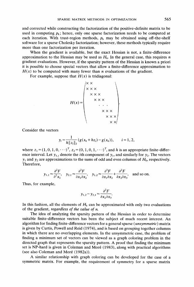
When the gradient is available, but the exact Hessian is not, a finite-differenceapproximation to the Hessian may be used as H. In the general case, this requires ngradient evaluations. However, if the sparsity pattern of the Hessian is known a prioriit is possible to choose special vectors that allow a finite-difference approximation toH(x) to be computed with many fewer than n evaluations of the gradient.

For example, suppose that H(x) is tridiagonal"

/

H(x)

XXX

XXX

XX

Consider the vectors

1Yi hit Zi112

(g(x + hzi)--g(Xk)), i= 1, 2,

where z (1, 0, 1, 0,. .) , z2 (0, 1,0, 1,. .) , and h is an appropriate finite-differ-ence interval Let Yl.i denote the ith component of Yl, and similarly for Y2. The vectors

Yl and. Y2 are approximations to the sums of odd and even columns of Hk, respectively.Therefore,

O2F O2F a2F 02F+, and so on.Y1,1 02Xl, Yz,I OXIOX2, Y,2

OXlfX2 OX2fX3

Thus, for example,

a2F

In this fashion, all the elements of H can be approximated with only two evaluationsof the gradient, regardless of the value of n.

The idea of analyzing the sparsity pattern of the Hessian in order to determinesuitable finite-difference vectors has been the subject of much recent interest. Analgorithm for finding finite-difference vectors for a general sparse (unsymmetric) matrixis given by Curtis, Powell and Reid (1974), and is based on grouping together columnsin which there are no overlapping elements. In the unsymmetric case, the problem offinding a minimum set of vectors can be viewed as a graph coloring problem in thedirected graph that represents the sparsity pattern. A proof that finding the minimumset is NP-hard is given in Coleman and Mor6 (1983), along with practical algorithms(see also Coleman and Mor6 (1982a)).

A similar relationship with graph coloring can be developed for the case of asymmetric matrix. For example, the requirement of symmetry for a sparse matrix


means that the associated column-interaction graph will be undirected. The problemof finding a minimum set of finite-difference vectors for a symmetric matrix is NP-complete (a proof for a particular symmetric problem is given in McCormick (1983);see also Coleman and Mor6 (1982b)). Nonetheless, effective algorithms have beendeveloped based on graph-theoretic heuristics. The algorithms are based on principlessimilar to those for the unsymmetric case, but are considerably complicated by exploit-ing symmetry.

A finite-difference Newton-type method for sparse problems thus begins with aprocedure that analyzes the sparsity pattern in order to determine suitable finite-difference vectors. Algorithms for finding these vectors have been given by Powell andToint (1979) and Coleman and Mor6 (1982b). Once a sparse finite-difference Hessianapproximation has been computed, a sparse factorization can be computed as with theexact Hessian.

2.3. Sparse quasi-Newton methods. Because of the great success of quasi-Newtonmethods on dense problems, it is natural to consider how such methods might beextended to take advantage of sparsity in the Hessian. This extension was suggestedfirst for the case of sparse nonlinear equations by Schubert (1970), and was analyzedby Marwil (1978). Discussions of sparse quasi-Newton methods for optimization andnonlinear equations are given in Toint (1977), Dennis and Schnabel (1979), Toint(1979), Shanno (1980), Steihaug (1980), Thapa (1980), Powell (1981), Dennis andMarwil (1982) and Sorensen (1982). In the remainder of this section we give a briefdescription of sparse quasi-Newton methods applied to unconstrained optimization.

In quasi-Newton methods for dense problems, the Hessian approximation Hk isupdated at each iteration by the relationship

H+ H + U.

The update matrices Uk associated with many dense quasi-Newton methods are ofrank two, and can be shown to be the minimum-norm symmetric change in Hk, subjectto satisfying the quasi-Newton condition

(2.3)

where Sk Xk+l--Xk and Yk gk+1--gk (see, e.g., Dennis and Mor6 (1977)). By suitablechoice of the steplength Ofk in (1.1), the property of hereditary positive-definitenesscan also be maintained (i.e., Hk+I is positive definite if Hk is). However, the updatematrices Uk do not retain the sparsity pattern of the Hessian.

The initial approach to developing sparse quasi-Newton updates was to imposethe additional constraint of retaining sparsity on the norm-minimization problem(Powell (1976); Toint (1977)). Let 3c be defined as the set of indices {(i, ])lHij(x) -0},so that represents the specified sparsity pattern of the Hessian, and assume that Hkhas the same sparsity pattern. A sparse update matrix Uk is then the solution of

minimize uIIu

(2.4)subject to (Hk + U)Sk Yk,

t =t:

Uij=O for(i,j)Ac.


Let r() denote the vector Sk with the sparsity pattern of the jth column of Hkimposed. When the norm in (2.4) is the Frobenius norm, the solution is given by

(2.5) Ukj-I

where ej is the jth unit vector and is the vector of Lagrange multipliers associatedwith the subproblem (2.4). The vector A is the solution of the linear system

(2.6) QA Yk HkSk,

where

Q (r)r()+ [[r()l122ei)e.j=l

The matrix Q is symmetric and has the same sparsity pattern as Hk; Q is positive-definite if and only if IIr(J)l] > 0 for all j. (The sparse analogue of any quasi-Newtonformula may be obtained using a similar analysis; see Shanno (1980) and Thapa (1980).)

Thus far, sparse quasi-Newton methods have not enjoyed the great success oftheir dense counterparts. First, there are certain complications that result from therequirement of sparsity. In particular, note that the update matrix Uk (2.5) is of rankn, rather than of rank two; this means that the new approximate Hessian cannot beobtained by a simple update of the previous approximation. Second, an additionalsparse linear system (2.6) must be solved in order to compute the update. Finally, itis not possible in general to achieve the property of hereditary pogitive-definitenessin the matrices {Hk} if the quasi-Newton condition is satisfied (see Toint (1979) andSorensen (1982)); in fact, positive-definiteness may not be retained even if Hk is takenas the exact (positive definite) Hessian and the initial Xk is very close to the solution(see Thapa (1980)).

In addition to these theoretical difficulties, computational results have tended toindicate that currently available sparse quasi-Newton methods are less effective thanalternative methods (in terms of the number of function evaluations required forconvergence). However, hope remains that their efficiency may be improvedmforexample, by relaxing the quasi-Newton condition (2.3), or by finding only an approxi-mate solution of (2.6) (Steihaug (1982)). For a discussion of some possible newapproaches, see Sorensen (1982).

2.4. Conjugate-gradient methods. The term conjugate-gradient refers to a classof optimization algorithms that generate directions of search without storing a matrix.They are essential in circumstances when methods based on matrix factorization arenot viable because the relevant matrix is too large or too dense. We emphasize thatthere are two types of conjugate-gradient methodsmlinear and nonlinear.

The linear conjugate-gradient method was originally derived as an iterative pro-cedure for solving positive-definite symmetric systems of linear equations (Hestenesand Stiefel (1952)). It has been studied and analyzed by many authors (see, e.g., Reid(1971)). When applied to the positive-definite symmetric linear system

(2.7) Hx -c,

it computes a sequence of iterates using the relation (1.1). The vector Pk is defined by

(2.8) Pk --(HXk + c) + flk-lPk-1,

and the step length ak is given by an explicit formula. The matrix H need not bestored explicitly, since it appears only in matrix-vector products.


With exact arithmetic, the linear conjugate-gradient algorithm will compute thesolution of (2.7) in at most m (m <= n) iterations, where m is the number of distincteigenvalues of H. Therefore, the number of iterations required should be significantlyreduced if the original system can be replaced by an equivalent system in which thematrix has clustered eigenvalues. The idea of preconditioning is to construct a transfor-mation to have this effect on H. One of the earliest references to preconditioning forlinear equations is Axelsson (1974). See Concus, Golub and O’Leary (1976) for detailsof various preconditioning methods derived from a slightly different viewpoint.

The nonlinear conjugate-gradient method is used to minimize a nonlinear functionwithout storage of any matrices, and was first proposed by Fletcher and Reeves (1964).In the Fletcher-Reeves algorithm, Pk is defined as in the linear case by (2.8), wherethe term Hxk + c is replaced by g, the gradient at x. For a nonlinear function, a in(1.1) must be computed by an iterative step-length procedure. When the initial vector

P0 is taken as the negative gradient and a is the step to the minimum of F along pk,

it can be shown that each p is a direction of descent for F.Many variations and generalizations of the nonlinear conjugate-gradient method

have been proposed. The most notable features of these methods are:/3 is computedusing different definitions; p is defined as a linear combination of several previoussearch directions; P0 is not always chosen as the negative gradient; and a is computedwith a relaxed linear search (i.e., ak is not necessarily a close approximation to thestep to the minimum of F along p). Furthermore, the idea of preconditioning maybe extended to nonlinear problems by allowing a preconditioning matrix that variesfrom iteration to iteration.

It is well known that rounding errors may cause even the linear conjugate-gradientmethod to converge very slowly. The nonlinear conjugate-gradient method displays arange of performance that has not yet been adequately explained. On problems inwhich the Hessian at the solution has clustered eigenvalues, a nonlinear conjugate-gradient method will sometimes converge more quickly than a quasi-Newton method,whereas on other problems the method will break down, i.e. generate search directionsthat lead to essentially no progress. For recent surveys of conjugate-gradient methods,see Gill and Murray (1979), Fletcher (1980) and Hestenes (1980).

2.5. The truncated linear conjugate-gradient method. Much recent interest hasbeen focussed on an approach to unconstrained optimization in which the equations(2.1) that define the search direction are "solved" (approximately) by performing alimited number of iterations of the linear conjugate-gradient method.

Consider the case in which the exact Hessian is used in (2.1). Dembo, Eisenstatand Steihaug (1982) note that the local convergence properties of Newton’s methoddepend on p being an accurate solution of (2.1) only near the solution of the uncon-strained problem. They present a criterion that defines the level of accuracy in pnecessary to achieve quadratic convergence as the solution is approached, and suggestsystematically "truncating" the sequence of linear conjugate-gradient iterates whensolving the linear system (2.1) (hence their name of "truncated Newton method").(See also Dembo and Steihaug (1980) and Steihaug (1980).)

This idea has subsequently been applied in a variety of situationsmfor example,in computing a search direction from (2.1) when H is a sparse quasi-Newton approxi-mation (Steihaug (1982)). We therefore prefer the more specific name of truncatedconjugate-gradient methods. These methods are useful in computing search directionswhen it is impractical to store Hk, but it is feasible to compute a relatively small numberof matrix-vector products involving H. For example, this would occur if Hk were the


product of several sparse matrices whose product is dense (see 3.3.1). Truncatedconjugate-gradient methods have also been used when the matrix-vector product Hkvis approximated (say, by a finite-difference along v); in this case, the computation ofpk requires a number of gradient evaluations equal to the number of linear coniugate-gradient iterations (see, e.g., O’Leary (1982)). In order for these methods to beeffective, it must be possible to compute a good solution of (2.1) in a small numberof linear conjugate-gradient iterations, and hence the use of preconditioning isimportant.

With a truncated coniugate-gradient method, complications arise when the matrix

H is not positive definite, since the linear coniugate-gradient method is likely to breakdown. Various strategies are possible to ensure that p is still a well-defined descentdirection even in the indefinite case. For example, the coniugate-gradient iterates maybe computed using the Lanczos process (Paige and Saunders (1975)); a Choleskyfactorization of the resulting tridiagonal matrix leads to an algorithm that is equivalentto the usual iteration in the positive-definite case. If the tridiagonal matrix is indefinite,a related positive-definite matrix can be obtained using a modified Cholesky factoriz-ation. Furthermore, preconditioning can be included, in which case the linear conjugate-gradient iterates begin with the negative gradient transformed by the preconditioningmatrix. If the preconditioning matrix is a good approximation to the Hessian, theiterates should converge rapidly. Procedures of this type are described in O’Leary(1982) and Nash (1982).

Further flexibility remains as to how the result of a truncated conjugate-gradientprocedure may be used within a method for unconstrained optimization. Rather thansimply being used as a search direction, for example, p may be combined with previoussearch directions in a nonlinear conjugate-gradient method (see Nash (1982)).

3. Linearly constrained optimization.3.1. Introduction. The linearly constrained problem will be formulated as

LCP minimize F(x)

subject to x b,

l<=x<_<_u,

where the m n matrix is assumed to be large and sparse. For simplicity, we assumethat the rows of are linearly independent (if not, some of them may be removedwithout altering the solution).

The most popular methods for linearly constrained optimization are active-setmethods, in which a subset of constraints (the working set) is used to define the searchdirection. The working set at x usually includes constraints that are satisfied exactlyat xk; the search direction is then computed so that movement along p will continueto satisfy the constraints in the working set.

With problem LCP, the working set will include the general constraints x- band some of the bounds. When a bound is in the working set, the correspondingvariable is fixed during that iteration. Thus, the working set induces a partition of xinto fixed and free variables.

We shall not be concerned with details of how the working set is altered, butmerely emphasize that the fixed variables at a given iteration are effectively removedfrom the problem; the corresponding components of the search direction will be zero,and thus the columns of corresponding to fixed variables may be ignored. Let Adenote the submatrix of corresponding to the free variables at iteration k; each


change in the working set corresponds to a change in the columns of Ak. Let nv denotethe number of free variables, and the vector Pk denote the search direction with respectto the free variables only.

By analogy with (2.2) in the unconstrained case, we may choose Pk as the stepto the minimum of a quadratic approximation to F, subject to the requirement ofremaining on the constraints in the working set. This gives Pk as the solution of thefollowing quadratic program:

minimize g[p + 1/2pTHkpp

(3.1)subject to Akp O,

where gk denotes the gradient and Hk the Hessian (or Hessian approximation) at Xkwith respect to the free variables.

The solution Pk and Lagrange multiplier Ak Of the problem (3.1) satisfy the nv + mequations

which will be called the augmented system.One convenient way to represent p involves a matrix whose columns form a basis

for the null space of A. Such a matrix, which will be denoted by Z, has nv-mlinearly independent columns and satisfies AZ 0. The solution of (3.1) may thenbe computed by solving the null-space equations

(3.3) Z2HkZkPz --Z2gk

and setting

(3.4) Pk Zkpz.

Equations (3.3) and (3.4) define a null-space representation of Pk (SO named becauseit explicitly involves Zk). The vector Zgk and the matrix ZHkZk are called theprojected gradient and projected Hessian.

3.2. Representation ot the null space. The issues that arise in representing Zkwhen Ak is sparse illustrate the need to compromise strategies that are standard fordense problems. In the rest of this section, we shall drop the subscript k associatedwith the iteration.

In dense problems, it is customary to use an explicit LQ or some other orthonormalfactorization of A in order to define Z. If AQ (L 0), where the orthonormal matrixQ is partitioned as (Y Z) and L is lower triangular, then AZ 0. In this case, Z hasthe "ideal" property that its columns are orthonormal, so that formation of theprojected Hessian and gradient does not exacerbate the condition of (3.3) and (3.4).Unfortunately, for large problems computation of such a factorization is normally tooexpensive. (Some current research is concerned with efficient methods for obtainingsparse orthogonal factorizations; see George and Heath (1981). However, the needto update the factors is an even more serious difficulty; see Heath (1982) and Georgeand Ng (1982).)

If an orthogonal factorization is unacceptable, a good alternative is to reduce Ato triangular form using Gaussian elimination (i.e., elementary transformations com-bined with row and column interchanges). This would give an LU factorization in the


form

I(L 0),

where P1 and P2 are permutation matrices, U is unit upper triangular, and L is lowertriangular. The matrices P1 and P2 would be chosen to make U well-conditioned andW]I reasonably small. The required matrix

would no longer have orthonormal columns, but should be quite well conditioned,even if A is poorly conditioned.

Unfortunately, it is not known how to update the factorization (3.5) efficiently inthe sparse case when columns of A are altered. However, (3.5) indicates the existenceof a square, nonsingular submatrix drawn from the rows and columns of A. We shallassume for simplicity that this matrix comprises the left-most columns of A, i.e.

(3.7) A=(B S),

where B is nonsingular. (In practice, the columns of B may occur anywhere in A.) Itfollows from (3.7) and (3.5) (with P1 and P2 taken as identity matrices) that BW+ S O,so that W =-B-1S. Thus, Z has the form

As long as B in (3.7) is nonsingular, the matrix Z (3.8) will provide a basis for thenull space of A. In the absence of the ideal factorization (3.5), the aim must be tochoose a B that is as well.conditioned as conveniently possible, since this will tend tolimit the size of wII and hence the condition of Z.

The partition of the columns of A given by (3.7) induces a partition of the freevariables, which will be indicated by the subscripts " and s". The rn variables xare called the basic variables. The remaining s free variables (s- nv- m) are calledthe superbasic variables. For historical reasons, the fixed variables are sometimes calledthe nonbasic variables.

An advantage of the form (3.8) for sparse problems is that operations with Z andZr may be performed using a factorization of the matrix B; the matrix Z itself neednot be stored. For example, the vector Zrg required in (3.3) may be written as

(3.9) Zrg=-SrB-rgn+gs.

(The vector on the right-hand side of (3.9) is called the reduced gradient; note that itis simply the projected gradient with a particular form of Z.) Thus, Zg may beobtained by solving Brv gn, and then forming gs-Srv. Similarly, to form p Zpz,we have

p=(-BI-1St pz.__(-B-1SPz,Pz /

which gives the system

BpB -Spz.


With the reduced-gradient form of Z (3.8), the problems of representing a nullspace and computing the associated projections reduce to the familiar operations offactorizing and solving with an appropriate square B.

3.3. Solving for the search direction. At each iteration of an active-set methodfor LCP, the search direction p with respect to the free variables solves the subproblem(3.1). We have seen that there are mathematically equivalent representations of p;the way in which p is computed for sparse problems depends on several considerations,which will be discussed below.

3.3.1. Solving the null-space equations. For sparse problems, it will generally notbe possible to solve (3.3) by explicitly forming and then factorizing ZTHZ. Even if Hand B are sparse, the projected Hessian will generally be dense. Thus, if a factorizationof the projected Hessian is to be stored, the number of superbasic variables at eachiteration must be sufficiently small (i.e., the number of fixed variables must besufficiently large). Fortunately, for many large-scale problems there is an a priori upperbound on the number of free variables. For example, if only q of the variables appearnonlinearly in the objective function, the dimension of the projected Hessian matrixat the solution cannot exceed q.

Furthermore, even if the dimension of Z’HZ is small, forming the projectedHessian may involve a substantial amount of work; when Z is defined by (3.8),computation of ZHZ requires the solution of 2s systems of size m m. For thisreason, a Newton-type method in which the projected Hessian is recomputed at eachiteration is not generally practical. By contrast, quasi-Newton methods can be adaptedvery effectively to sparse problems in which the dimension of the projected Hessianremains small, by updating a dense Cholesky factorization of a quasi-Newton approxi-mation to the projected Hessian; this is the method used in the MINOS code of Murtaghand Saunders (1977), (1980).

When the projected Hessian cannot be formed or factorized, the null-spaceequations may be solved using an iterative method that does not require storage ofthe matrix, such as a truncated conjugate-gradient method (see 2.5). In order forthis approach to be reasonable, the computation of matrix-vector products involvingZ and H must be relatively cheap (e.g., when H is sparse); in addition, a goodapproximation to the solution of (3.3) must be obtained in a small number of iterations.Even when the Hessian is not available, a truncated conjugate-gradient method maybe applied to (3.3) by using a finite-difference of the gradient to approximate thevector HZv; an evaluation of the gradient is thus necessary for every iteration of thetruncated conjugate-gradient method. Note that this is one of the few methods inwhich H is not required to be sparse.

Each of the above methods for solving the null-space equations can be adaptedto allow for changes in the working set ( 3.5).

3.3.2. Solving the range-space equations. The null-space equations provide onemeans of solving for p in the augmented system (3.2), by eliminating &k. When H ispositive definite, a complementary approach is to solve for & first, via the range-spaceequations

AH-1AT" AH-Ig, Hp AT" g.

This method would be appropriate if H were sparse, and if A had relatively few rows.The application of a range-space approach to quadratic programming is discussed byGill et al. (1982).


3.3.3. Solving the augmented system. An alternative method for obtaining pinvolves treating the augmented system directly. (Variations of this idea have beenproposed by numerous authors; see, e.g., Bartels, Golub and Saunders (1970)). Themost obvious way to solve (3.2) is to apply a method for symmetric indefinite systems,such as the Harwell code MA27 (Duff and Reid (1982)). In order for the solution of(3.2) to be meaningful, the matrix ZTHZ must be positive definite. Verifying positive-definiteness in this situation is a nontrivial task, since of course the matrix ZTHZ isnot computed explicitly. However, the result may sometimes be known a priorimforexample, when H itself is positive-definite.

Both H and A change dimension when the working set is altered. Updatingprocedures for this case are discussed in 3.6.2.

3.4. Factorizing and solving a square system. The linear systems involving B andB are typically solved today using a sparse LU factorization of B. Surveys oftechniques for computing such a factorization are given in Duff (1982) and Duff andReid (1983). The analyze phase of a factorization consists of an analysis of the sparsitypattern alone (independent of the values of the elements), and leads to a permutationof the matrix in order to reduce fill-in during the factorization. The factorphase consistsof computation with the actual numerical elements of the matrix.

We shall mention a few features of certain factorization methods that haveparticular relevance to optimization (see Duff and Reid (1983) for more details). Sinceactive-set algorithms include a sequence of matrices that undergo column changes, thefactorization methods were typically developed to be used in conjunction with anupdate procedure.

The p4 algorithm of Hellerman and Rarick (1971), (1972) performs the analyzephase separately from the factor phase, and produces the well-known "bump andspike" structure, in which B is permuted to block lower-triangular form with relativelyfew "spikes" (columns containing nonzeros above the diagonal). This procedure isvery effective if B is nearly triangular. Also, the factor phase is able to use externalstorage, since it processes B one column at a time. Column interchanges are used tostabilize the factorization. (Row interchanges would destroy the sparsity pattern.) Ifan interchange is needed at the ith stage, it is necessary to solve a system of the formL/_ly ei and to compute the quantities yTaj for all remaining eligible spike columnsaj. This involves significant work and also degrades the sparsity of the factors. Thus,a rather loose pivot tolerance must be used to avoid many column interchanges (e.g.,I/zl < 104, where/x is the largest subdiagonal element in any column of L divided bythe corresponding diagonal).

The Markowitz algorithm (Markowitz (1957)), on the other hand, performs theanalyze and factor phases simultaneously, and hence must run in main memory. Itcomputes dynamic "merit counts" in order to determine the row and column permuta-tions to preserve sparsity and yet retain numerical stability. The Markowitz procedurecan achieve a good sparse factorization even with a rather strict pivot tolerance (e.g.,

In order to indicate how these factor routines perform on matrices that arise inoptimization, we give results on five test problems. In the first three problems, thematrix B has "staircase" structure (see, e.g., Fourer (1982)); constraints of this formoften arise in the modeling of dynamic systems, in which a set of activities is replicatedover several time periods. The fourth and fifth problems arise from the optimal powerflow (OPF) problem (see e.g., Stott, Alsac and Marinho (1980)). In this case, B is theJacobian of the network equations of the power system, and has a symmetric sparsity


TABLESummary of problem characteristics.

Stair Stair 2 Stair 3 OPF OPF 2

B rows 357 745 1,170 1,200 3,400

B nonzeros 3,500 3,600 7,100 9,000 29,000

p4 blocks 5 13

p4 spikes 66 101 157 715

pattern (which is not at all triangular!) Table 1 shows some of the relevant featuresof the problems described, including the results of factorization with the p4 algorithm.

The number of nonzeros in the initial LU factorization of B is shown in the firsttwo rows of Table 2. The p4 algorithm is as implemented in the MINOS code ofMurtagh and Saunders (1977), (1980); the Markowitz procedure is the Harwell codeLA05 (Reid (1976), (1982)). Note that the large number of spikes in the first OPFproblem is bound to cause difficulties for the p4 algorithm.

TABLE 2Number of nonzeros in initial LU factorization and after k updates.

Stair Stair 2 Stair 3 OPF OPF 2

LoUo with p4 (MINOS) 9,400 16,200 32,000 30,400

LoUo with Markowitz (LA05) 5,400 4,700 13,500 13,800 75,000

k 50 50 50 30 40

L U with LA05 7,800 6,000 17,100 15,300 83,000

3.5. Column updates. For problems of the form LCP, each change in the workingset involves changing the status of a variable from fixed to free (or vice versa). Whena previously fixed variable becomes free, a column of is added to A; this poses noparticular difficulty, since the new column can simply be appended to S. When a freevariable is to become fixed, a column of A must be deleted, and complications ariseif the column is in B. Since the number of columns in B must remain constant (inorder for B to be nonsingular), it is necessary to replace a column of B with one ofthe columns of S.

Assume that we are given an initial B0, which thereafter undergoes a sequenceof column replacements, each corresponding to one of the free variables becomingfixed on a bound. Let Ik denote the index of the column to be replaced at the kthstep, ak denote the lkth column of B, Vk denote the new column, and el denote thelkth column of the identity matrix. After each replacement, we have

(3.10) Bk Bk-1 + Vk ak)e.

We shall consider several ways in which systems of equations involving Bk can besolved following a sequence of such changes.


3.5.1. The product-form update. The standard updating technique used in allearly sparse LP codes was the product-form (PF) update (e.g., Dantzig and Orchard-Hays (1954)). It follows from the definition of Bk that

B B_ T,

whereT(3.11) Bk_lY v and T I + y elk) e

Note that Tk is a permuted triangular matrix (with only one nontrivial column);equivalently, T is a rank-one modification of the identity matrix. The matrix T canbe represented by storing the index l and the vector

After k such updates we have

(3.12) B BoTIT2"" Tk.

Given a procedure to solve systems of equations involving Bo, (3.12) indicates thatsolving Bv b is equivalent to solving the k + 1 linear systems

(3.13) Bovo=b, Tv=vo, ..., Tvk=v_

where the systems involving T are easy to solve. As k increases, the solution processbecomes progressively more protracted, and the storage required to store the updatesis strictly increasing. Therefore it becomes worthwhile to compute a factorization ofB from scratch. Most current systems use an initial triangular factorization Bo Lo Uo(see 3.4), and recompute the factorization after k updates (typically k _-< 50).

The PF update has two important advantages for sparse problems. First, thevectors {y} may be stored in a single sequential file, so that implementation isstraightforward. Second, any advance in the methods for linear equations is immediatelyapplicable to the factorization of Bo, since the update does not alter the initialfactorization. Thus, Bo may be represented by a "black box" procedure for solvingequations (involving both Bo and BoT).

Unfortunately, the PF update has two significant deficiencies. It is numericallyTunreliable if lelkykl is too small (since T is then ill-conditioned), and the growth of

data defining the updates is significantly greater than for alternative schemes.

3.5.2. The Bartels-Golub update. The instability of the PF update was first madeprominent by Bartels and Golub (1969), who showed as an alternative that an LUfactorization can be updated in a stable manner (see also Bartels, Golub and Saunders(1970); Bartels (1971)). Given an initial factorization Bo=LoUo, the updates to Lare represented in product form, but the sparse triangular matrix U is stored (andupdated) explicitly. Thus, instead of the form (3.12) we have

(3.14) B LoT1 T2 TqUt =- LU,

where each T represents an update whose construction will be discussed below.At the kth step, replacing the /th column of B-I gives

B L_ U,

where /_) is identical to Uk-1 except for its /th column. Since Uk-1 is stored as asparse matrix, it is desirable to restore U to upper-triangular form U without causingsubstantial fill-in. To this end, let P denote a cyclic permutation that moves the /throw and column of U to the end, and shifts the intervening rows and columns forward.


We then have

pT/p

The nonzeros in the bottom row of PTIQP may be eliminated by adding multiplesof the other rows. However, it follows from the usual error analysis of Gaussianelimination (e.g., Wilkinson (1965)) that this procedure will not be numerically stableunless the size of the multiple is bounded in some way. Hence, we must allow the lastrow to be interchanged with some other row. Formally, the row operations are stabilizedelementary transformations (Wilkinson (1965)), which are constructed from 22matrices of the form

or /--1 1 x

(Note that the transformation//includes a row interchange.) Each such transformationis represented by the scalar x, and is unnecessary if the element to be eliminated isalready zero. Numerical stability is achieved by choosing between M and//so thatthe multiplier x is bounded in size by some moderate number (e.g., Ixl <- 1, 10 or100). The matrices {T} in (3.14) are constructed from sequences of matrices of theform (3.15).

Unfortunately, elimination of the nonzeros is easier said than done" in the sparsecase. Any transformation of type r amounts to a form of fill-in, since the location ofnonzeros in the interchanged rows is unlikely to be the same. A complex data structureis therefore needed to update U without losing efficiency during subsequent solves.(Holding individual nonzeros in a linked list, for example, would not be acceptable ina virtual-memory environment.)

The implementation of the BG update by Saunders (1976) capitalizes on thebump and spike" structure revealed by the p4 procedure (see 3.4). Each triangularfactor is of the form

and fill-in can occur only within Fk. If Uo contains s spikes, the dimension of Fk willbe at most s + k. Storing F as a dense matrix allows the BG update to be implementedwith maximum stability (11--< 1 in (3.15)), and the approach is efficient as long as sis not unduly large (say, s-< 100). This implementation has been used for several yearsin the nonlinear programming system MINOS (Murtagh and Saunders (1977), (1980)).During that period, the number of spikes in U0 has proved to be favorably small formany sparse optimization models. However, two important applications are now knownto give unacceptably large numbers of spikes: time-period models (for which B has astaircase structure) and optimal power-flow problems (for which B has a symmetricsparsity pattern). Some statistics for these problems are given in Table 1 ( 3.4).


Another implementation of the BG update has been developed by Reid (1976),(1982) as the Fortran package LA05 in the Harwell Subroutine Library. It strikes acompromise between dense and linked-list storage by using a whole row or columnof Uk as the "unit" of storage. Thus, the nonzeros in any one row of Uk are held incontiguous locations of memory, as are the corresponding column indices, and anordered list points to the beginning of each row. To facilitate searching, a similar datastructure is used to hold just the sparsity pattern of each column (i.e., the row indicesare stored, but not the nonzeros themselves; see Gustavson (1972)). This storagescheme is also suitable for computing an initial LU factorization using the Markowitzcriterion and threshold pivoting--a combination that has been eminently successful inpractice, particularly on the structures mentioned above. Table 2 ( 3.4) shows thesparsity of various initial factorizations B0 LoUo computed by subroutine LA05A,and the moderate rate of growth of nonzeros following k calls to the BG updatesubroutine LA05C.

Given the row-wise storage scheme for the nonzeros of Uo, it was natural inLA05A for the stability test to be applied row-wise. (Thus, each diagonal of U0 mustnot be too small compared to other nonzeros in the same row.) This standard thresholdpivoting rule is appropriate for single systems, but unfortunately is at odds with theaim of the BG update. The effect is to control the condition of U0, with no controlon the size of the multipliers/x defining L0.

A preferable alternative is to apply the threshold pivoting test column-wise, inorder to control the condition of L0. The resulting Lo, and hence all subsequent factorsLk, will then be a product of stabilized transformations T. It follows that the factorsof Bk are likely to be well conditioned if Bk is well conditioned, even if Bo is not.

In order to apply the column-wise stability test efficiently, the data structure forcomputing U0 needs to be transposed. This and other improvements will be incorpor-ated in a new version of LA05 (Reid, private communication).

At the Systems Optimization Laboratory we have recently implemented someanalogous routines as part of a package LUSOL, which will maintain the factorizationLkBk--Uk following various kinds of updates. The matrices Bk may be singular orrectangular, and the updates possible are column replacement, row replacement,rank-one modification, and addition or deletion of a row or a column. The conditionof Lk is controlled throughout for the reasons indicated above. We expect such apackage to find many applications within optimization and elsewhere. One examplewill be to maintain a sparse factorization of the Schur-complement matrix Ck (see

3.5.4-3.6.2), often called the working basis in algorithms for solving mathematicalprograms that have special structure. GUB rows and imbedded networks are examplesof such structure; see Brown and Wright (1981) for an excellent overview.

3.5.3. The Forrest-Tomlin update. The update of Forrest and Tomlin (1972)was developed as a means of improving upon the sparsity of the PF update whileretaining the ability to use external storage where necessary. In fact the FT update isa restricted form of the BG update, in which no row interchanges are allowed wheneliminating the bottom row of pTOp. This single difference removes the fill-in difficulty(but at the expense of losing guaranteed numerical stability).

Algebraically, a new column Wk is added to Uk-1, the Ikth column and row aredeleted, and the transformations M are combined into a single "row" transformationRk I + e rk elk) T. It can be shown that the required vectors satisfy

(3.16) Lk-l Wk Vk, and U-lrk elk,


and the new diagonal of Uk is rTWk Most importantly, the multipliers tz are closelyrelated to the elements of rk, and these can be tested a posteriori to determine whetherthe update is acceptable (see also Tomlin (1975)). In practice a rather undemandingtest such as [tzl -< 106 must be used to avoid rejecting the update too frequently. TheFT update is now used within several commercial mathematical programming systems.

3.5.4. Use of the Schur complement. The work of Bisschop and Meeraus (1977),(1980) has recently provided a new perspective on the problem of updating withinactive-set methods. Suppose that for each update a vector vj replaces the/jth columnof B0. A key observation is that the system BkX b is equivalent to the system

(3.17) (B0 Vk)where

Vg (/)1/)2"" Vk), I (el, el2"’" elk) T.Note that the rectangular matrix I is composed of k rows of the identity matrixcorresponding to indices of columns that have been replaced. Since the equationsIky 0 set k elements of y to zero, the remaining elements of y and z together givethe required solution x. Similarly, the system B[y d is equivalent to

if d and d; are constructed from d appropriately (with the aid of k arbitrary elements,such as zero).

The matrix in (3.17) may be factorized in several different ways. In the next twosections we consider the simplest factorization

(3.19) (BVk)where

(.a0) B0Y , C -IThe k x k matrix C is the Schur complement for the partitioned matrix on the left-handside of (3.19). It corresponds to a matrix of the ubiquitous form D-WB-V (e.g.,see Cottle (1974)).

3... slee-e. From (3.17) and (3.19) we see that thevectors y and z needed to construct the solution of Bx b may be obtained fromthe equations

(3.21a) Bow b,

(.b) Cz -,(3.21c) y w- Yz.Similarly, the solution of By d is obtained from the two linear systems

(.al c2z -(3.22b) Bgy=d-I2z.

Assuming that Y is available, the essential operations in (3.21) and (3.22) are a solve


with Bo and a solve with Ck. If k is small enough (say, k-<_ 100), Ck may be treatedas a dense matrix. It is then straightforward to use an orthogonal factorization QkCkRk Q Qk L Rk upper triangular) or an analogous factorization LkCk Uk based onGaussian elimination (Lk square, Uk upper triangular). These factorizations can bemaintained in a stable manner as Ck is updated to reflect changes to Bk. (The updatesinvolve adding and deleting rows and columns of Ck; see Gill et al. (1974).) Thestability of the procedures (3.21) and (3.22) then depends essentially on the conditionof Bo. In other words, if B0 is well conditioned, we have a stable method for solvingBkX b for many subsequent k.

The method retains several advantages of the PF update. The vectors to be stored(columns of Yk) satisfy BoYk Vk, which is analogous to (3.11). These vectors shouldhave sparsity similar to those in the PF update, and they can be stored sequentially(in compact form on an external file, if necessary). A further advantage is that whenevera column of Ck is deleted, the corresponding vector Yk may be skipped in subsequentuses of (3.21c). This gain would tend to offset the work involved in maintaining thefactors of Ck. Because of the parallels, the method described here amounts to a practicalmechanism for stabilizing an implementation based on the PF update.

3.5.6. The Schur-complement update. One of the aims of Bisschop and Meeraus(1977), (1980) was to give an update procedure whose storage requirements wereindependent of the dimension of B0. This is achievable because the matrix Yk is notessential for solving (3.17) and (3.18), given Vk and a "black box" for Bo. For example,(3.2 lc) may be replaced by

(3.23) Boy b- VkZ,

and hence storage for Yk can be saved at the expense of an additional solve with B0.Similarly, (3.22a) is equivalent to

Bw=dl, Cz=d2-V[w,

again involving a second solve with B0. Note that the original data Vk will usually bemore sparse than Yk, SO that the additional expense may not be substantial.

The storage required for a dense orthogonal factorization of Ck (k:z) is small formoderate values of k. As with the PF update, any advance in solving linear equationsis immediately applicable to the equations involving B0.

The method is particularly attractive when B0 has special structure. For example,certain linear programs have the following form"

minimize cTXsubject to (B0 N)x b,

l<_x<-u,where B0 is a square block-diagonal matrix"

B0 block-diag (Do D1 DN).

Assuming that the square matrices Dj are well conditioned, B0 provides a naturalstarting basis for the simplex method.

With the Schur-complement (SC) update, an iteration of the simplex method onsuch a problem requires four solves with B0, and hence four solves with each matrixDj. In certain applications, the matrices D are closely related to Do (e.g., in time-dependent problems), in which case a further application of the Schur-complementtechnique would be appropriate. A simplex iteration then involves only solves with Do.


This is a situation in which one factorization is followed by hundreds or eventhousands of solves (involving both Do and Dff). Thus, it is useful for black-box solversto be tuned to the case of multiple right-hand sides.

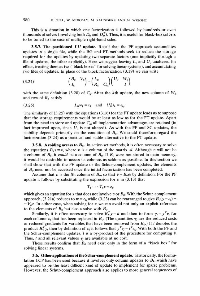
3.5.7. The partitioned LU update. Recall that the PF approach accumulatesupdates in a single file, while the BG and FT methods seek to reduce the storagerequired for the updates by updating two separate factors (one implicitly through afile of updates, the other explicitly). Here we suggest leaving L0 and U0 unaltered (ineffect, treating them as two "black boxes" for solving linear systems), and accumulatingtwo files of updates. In place of the block factorization (3.19) we can write

with the same definition (3.20) of C. After the kth update, the new column of Wand row of R satisfy

(3.25) Low v and Ur el.

The similarity of (3.25) with the equations (3.16) for the FT update leads us to supposethat the storage requirements would be at least as low as for the FT update. Apartfrom the need to store and update C, all implementation advantages are retained (infact improved upon, since U0 is not altered). As with the PF and SC updates, thestability depends primarily on the condition of Bo. We could therefore regard thefactorization (3.24) as a practical and stable alternative to the FT update.

3.5.8. Avoiding access to Bo. In active-set methods, it is often necessary to solvethe equations Bx v, where v is a column of the matrix . Although v will not bea column of B, it could be a column of B0. If B0 were not stored in main memory,it would be desirable to access its columns as seldom as possible. In this section weshall show that with the PF update or the Schur-complement updates, the elementsof B0 need not be accessed once the initial factorization has been completed.

Assume that v is the/th column of B0, so that v Boel by definition. For the PFupdate it follows by substituting the expression for v in (3.13) that

TI Tkx el,

which gives an equation for x that does not involve v or B0. With the Schur-complementapproach, (3.21a) reduces to w e, while (3.23) can be rearranged to give Bo(y- et)-Vz. In either case, when solving for x we can avoid not only an explicit referenceto the elements of B0 but also a solve with B0.

Similarly, it is often necessary to solve By d and then to form yrv foreach column v that has bee replaced in B0. (The quantities are the reduced costsor reduced gradients for variables that have been removed from B0.) If denotes theproduct By, then by definition of v it follows that yTv trec With both the PF andthe Schur-complement updates, is a by-product of the procedure for computing y.Thus, and all relevant values ) are available at no cost.

These results confirm that B0 need exist only in the form of a "black box" forsolving linear systems.

3.6. Other applications of the Sehur-eomplement update. Historically, the formu-lation LCP has been used because it involves only column updates to B, which haveappeared to be the least diNcult kind of update to implement for sparse problems.However, the Schur-complement approach also applies to more general sequences of


related square systems. As with column replacement, the key is to solve a partitionedsystem that involves the original matrix.

3.6.1. Unsymmetric rank-one updates. Consider the case in which Bo undergoesa sequence of rank-one modifications:

Bk Bk- + vks Bo + VkS.The solution of BkX-" b is part of the solution of the extended system

(3.26) (B0 :;)(:)(0(Kron (1956), Bisschop and Meeraus (1977)). Given factorizations of B0 and theSchur complement Ck =-I-SB- Vk, the solution may be obtained from

CkZ =-Sw, Box b- Vkz,

where Bow b. An alternative that would require more storage but less work couldbe obtained by using Bo Lo U0 and storing the vectors defined by LoLet Rk denote the matrix whose jth column is rj, and similarly for Wk. In this case,the solution of (3.26) would be obtained from

Ckz =-Rv UoX 1)- Wkz

where Lov b. Either approach is an alternative to updating a factorization of Bk itself(e.g., Gille and Loute (1981), (1982)), which is even more difficult to implement thanthe BG update.

We emphasize that column or row replacements are best treated as a special case,not as a sequence of general rank-one modifications.

3.6.2. A symmetric Schur-complement update. It was observed in 3.1 that insome circumstances the search direction can be computed by solving the linear system(3.2) involving the augmented matrix

(3.27) Mk=Ak

Within an active-set method, changes in the status of fixed and free variables lead tochanges in H and A. When a variable becomes fixed, the corresponding row andcolumn of Mk are deleted; when a variable is freed, a new row and column of Mk areadded.

Instead of updating a factorization of Mk, we can start with some M0 and workwith an augmented system of the form

If a variable is fixed at the kth change, the kth column of Sk is an appropriate coordinatevector; if the /th variable is freed, the column is

(h,)Skat

where ht is obtained from the/th column of the full Hessian, and at is the/th columnof s. The solution of the augmented system corresponding to the kth working set canthen be obtained using a factorization of M0 and a factorization of the Schur comple-ment Ck SM-

582 P. GILL, W. MURRAY, M. SAUNDERS AND Mo WRIGHT

3.7. Linear and quadratic programming. Two important special cases of LCP arelinear and quadratic programs. Since there are no user-supplied functions, the computa-tion in linear and quadratic programming methods involves primarily linear algebraicoperations.

3.7.1. Large-scale linear programming. Large-scale linear programs occur inmany important applications, such as economic planning and resource allocation.Methods and software for large-scale LP have thus achieved a high level of sophistica-tion, and many of the techniques discussed in 3 were designed originally for usewithin the simplex method.

Much research has involved linear programs with special structure in the constraintmatrix--for example, those arising from networks or time-dependent systems. It isimpossible to summarize methods for specially-structured linear programs in a surveypaper of this type. However, to illustrate the flavor of the work, we consider staircaselinear programs (which were used in the examples of 3.4). These arise in modelingtime-dependent processes; the recent book edited by Dantzig, Dempster and Kallio(1981) is entirely devoted to such problems. It has long been observed that the simplexmethod tends to be less efficient on staircase problems than on general LPs. To correctthis deficiency, work has tended to proceed in two directions. First, the simplex methodcan be adapted to take advantage of the staircase structure, by using special techniquesfor factorizing, updating, and pricing (Fourer (1982)). Second, special-purpose methodscan be designed to exploit particular features of the problem. For staircase problems,several variations of the decomposition approach (Dantzig and Wolfe (1960)) havebeen suggested. The basic idea is to solve the problem in terms of smaller, nearlyindependent, subproblems.

3.7.2. Large-scale quadratic programming. /k general statement of the quadraticprogramming problem is

minimize c TX + 1/2X THx

subject to x b,

l<=x<=u,

where H is a symmetric matrix.An early approach to quadratic programming was to transform the problem into

a linear program, which is then solved by a modified LP method (e.g., Beale (1967)).The most popular quadratic programming algorithms are now based on the active-setapproach described in 3.1 (for a comprehensive survey of QP methods, see Cottleand Djang (1979)), and the search direction is defined by the subproblem (3.1).Efficient methods for sparse quadratic programs thus involve specializing the techniquesdiscussed in 3.3 for the special case when the Hessian is constant.

4. Nonlinearly constrained optimization. The nonlinearly constrained optimiz-ation problem is assumed to be of the following form:

NCP minimize F(x)

subject to c(x)= O,

l<=x<-u,

where c(x) is a vector of m nonlinear constraint functions. We shall assume that these


constraints are "sparse", in the sense that the m x n Jacobian matrix A(x) of c(x) issparse. For simplicity, we shall usually not distinguish between linear and nonlinearconstraints in c(x). However, it is usually considered desirable to treat linear andnonlinear constraints separately.

Problems with nonlinear constraints are considerably more difficult to solve thanthose with only linear constraints. There is an enormous literature concerning methodsfor nonlinear constraints; recent overviews are given in Fletcher (1981) and Gill,Murray and Wright (1981). In this section, we shall concentrate on the impact ofsparsity rather than attempt a thorough discussion of the methods.

One aspect of NCP that is directly relevant to sparse matrix techniques is thatany superlinearly convergent algorithm must consider the curvature of the nonlinearconstraint functions, and thus the Hessian of interest is the Hessian of the Lagrangianfunction rather than the Hessian of F alone. Let the Hessian of the Lagrangian functionbe denoted by W(x, A) H(x)-i_ AiHi(x), where Hi is the Hessian of Ci. At first,it might appear unlikely that this matrix would be sparse, since it is a weighted sumof the Hessians of the objective function and the constraints. However, sparsity in thegradient of a nonlinear constraint always implies sparsity in its Hessian matrix. Forexample, if the gradient of c(x) contains five nonzero components, the correspondingHessian matrix H(x) can have at most 25 nonzero elements. Furthermore, there isoften considerable overlap in the positions of nonzero elements in the Hessians ofdifferent constraints. Thus, in practice the Hessian of the Lagrangian function is oftenvery sparse.

The usual approach to solving NCP is to construct a sequence of unconstrainedor linearly constrained subproblems whose solutions converge to that of NCP. Earlymethods included unconstrained subproblems based on penalty and barrier functions(see Fiacco and McCormick (1968)). Unfortunately, these methods suffer from inevi-table ill-conditioning; they have for the most part been superseded by more efficientmethods.

4.1. Augmented Lagrangian methods. Augmented Lagrangian methods weremotivated in large part by the availability of good methods for unconstrained optimiz-ation. The original idea was to minimize an approximation to the Lagrangian functionthat has been suitably augmented (by a penalty term) so that the solution is a localunconstrained minimum of the augmented function (Hestenes (1969), Powell (1969)).

In particular, an augmented Lagrangian method can be defined in which Xk/l istaken as the solution of the subproblem

minimize LA x, Ak, Pk

(4.1)subject to -<_ x _-< u,

where the augmented Lagrangian function LA is defined by

P(4.2) LA(X,A,p)=--F(x)--ATc(x)+-C(x)Tc(x).The vector A is an estimate of the Lagrange multiplier vector, and p is a suitablychosen nonnegative scalar. Alternatively, it is possible to treat any general linearconstraints by an active-set method ( 3.1), and to include only nonlinear constraintsin the augmented Lagrangian function. Whatever the definition of the subproblem,the algorithm has a two-level structure"outer" iterations (corresponding to differentsubproblems) and "inner" iterations (within each subproblem).


The Hessian of interest when solving (4.1) is the Hessian of LA (4.2), which isW(x, k)+pkA(x)TA(x). The sparsity patterns of W(x, ,) and the Hessian matrix ofLA are sometimes very similar. Hence, techniques designed to use an explicit sparseHessian may be applied to (4.1).

The Jacobian matrix A(x) need not be stored explicitly in order to solve thesubproblem (4.1). If a fairly accurate solution of (4.1) is computed, an improvedLagrange multipler estimate may be obtained without solving any linear systemsinvolving A(x). However, in several recent augmented Lagrangian methods, (4.1) issolved only to low accuracy in order to avoid expending function evaluations whenAk is a poor estimate of the optimal multipliers;, in this case, some factorization of thematrix A(x+l) is required to obtain an improved Lagrange multiplier estimate (bysolving either a linear system or a linear least-squares problem). The relevance of thestorage needed for the Jacobian and/or a factorization depends on the number ofnonlinear constraints and the sparsity of the Jacobian.

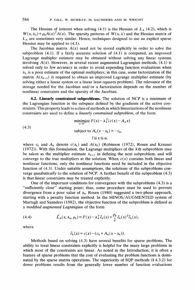
4.2. Linearly constrained subproblems. The solution of NCP is a minimum ofthe Lagrangian function in the subspace defined by the gradients of the active con-straints. This property leads to a class of methods in which linearizations of the nonlinearconstraints are used to define a linearly constrained subproblem, of the form

(4.3)

minimize F(x) A kr

C(X) AkX)

subject to A(x- x) -c,

where ck and A denote c(x) and A(x) (Robinson (1972), Rosen and Kreuser(1972)). With this formulation, the Lagrange multipliers of the kth subproblem maybe taken as the multiplier estimate ;tk/l in defining the next subproblem, and willconverge to the true multipliers at the solution. When c(x) contains both linear andnonlinear functions, only the nonlinear functions need be included in the objectivefunction of (4.3). Under suitable assumptions, the solutions of the subproblems con-verge quadratically to the solution of NCP. A further benefit of the subproblem (4.3)is that linear constraints may be treated explicitly.

One of the important conditions for convergence with the subproblems (4.3) is a"sufficiently close" starting point; thus, some procedure must be used to preventdivergence from a poor value of x0. Rosen (1980) suggested a two-phase approach,starting with a penalty function method. In the MINOS/AUGMENTED system ofMurtagh and Saunders (1982), the objective function of the subproblem is defined asa modified augmented Lagrangian of the form

pk(4.4) LA(X, Ak, Pk) F(X)- A k(X) +-- k(X) Tk(X),

where

k(X) C(X)--(Ck + Ak(X-- Xk)).

Methods based on solving (4.3) have several benefits for sparse problems. Theability to treat linear constraints explicitly is helpful for the many large problems inwhich most of the constraints are linear. As noted in the Introduction, it is often afeature of sparse problems that the cost of evaluating the problem functions is domi-nated by the sparse matrix operations. The superiority of SQP methods ( 4.3.2) fordense problems results from the generally lower number of function evaluations


compared to methods based on (4.3); for sparse problems, however, the functionevaluations required to solve (4.3) may be insignificant compared to the savings thatwould result from solving fewer subproblems. If an active-set method of the typedescribed in 3.3.1 is applied to (4.3), only the projected Hessian needs to be stored(rather than the full Hessian). Thus, methods based on (4.3) will tend to be moreeffective than augmented Lagrangian methods for problems in which the Hessian ofthe Lagrangian function is not sparse and the projected Hessian can be stored as adense matrix.

4.3. Methods based on linear and quadratic programming. We now consider twoclasses of methods in which the subproblems are solved without evaluation of theproblem functions (in contrast to the methods of 4.1 and 4.2).

4.3.1. Sequential linear programming methods. Because of the availability andhigh quality of software for sparse linear programs, a popular technique for solvinglarge-scale problems has been to choose each iterate as the solution of an LP subprob-lem; we shall call these sequential linear programming (SLP) methods. They were firstproposed by Griffith and Stewart (1961); for a recent survey, see Palacios-Gomez,Lasdon and Engquist (1982).

One crucial issue in an SLP method is the definition of the linear functions in thesubproblem. A typical formulation is

minimize g’(x x)

subject to Ak(x- xk) -c,

l<=x<_u.

With some formulations, the LP may not be well posedfor example, there may befewer constraints than variables. The usual way of ensuring a correctly posed subprob-lem is to include additional constraints on the variables, such as bounds on the changein each variable. In general, the latter are also needed to ensure convergence.

SLP methods have the advantage that the subproblems can be solved using allthe technology of sparse LP codes. They tend to be efficient on two types of problems:those with nearly linear functions, particularly slightly perturbed linear programs; andthose in which the functions can be closely approximated by piecewise linear functions(e.g., the objective function is separable and convex). Unfortunately, on generalproblems SLP methods are at best linearly convergent unless the number of activeconstraints at the solution is equal to the number of variables. Furthermore, the speedof convergence critically depends on the technique that defines each subproblem.

Recently, some of the techniques used in SQP methods ( 4.3.2) have been appliedto the SLP approachsuch as the use of a merit function to ensure progress aftereach outer iteration. Such techniques cannot be expected to improve the asymptoticrate of convergence of SLP methods, but they should improve robustness and overalleffectiveness.

Beale (1978) has given a method that is designed to make extensive use of anexisting LP system. The nonlinearly constrained problem is assumed to be of the form

minimize c(x)X,y

(4.5) subject to A(x)y-- b(x),

l<=x<=u,

v<=y<-w.


A special nonlinear algorithm is then used to adjust x; for each value of x, a newestimate y is determined by solving an LP.

4.3.2. Sequential quadratic programming methods. The most popular methodsin recent years for dense nonlinearly constrained problems are based on solving asequence of quadratic programming subproblems (see Powell (1982) for a survey).At iteration k, a typical QP subproblem has the form

minimize 1/2p rHkp + gp

subject to Akp =--Ck

l- xk <= p <- u Xk,

where Hk is an approximation to the Hessian of the Lagrangian function. The solutionof the QP subproblem is then used as the search direction p in (1.1). The step a ischosen to achieve a suitable reduction in some merit function that measures progresstoward the solution. In the dense case, the most popular method is based on takingH as a positive-definite quasi-Newton approximation to the Hessian (Powell (1977)).However, the many options in defining the QP subproblem have yet to be fullyunderstood and resolved (see Murray and Wright (1982), for a discussion of some ofthe critical issues).

Further complex issues are raised when applying an SQP method to sparseproblems (see, e.g., Gill et al. (1981)). The general development of methods has beenhampered because methods for sparse quadratic programming are only just beingdeveloped, and are not yet generally available for use within a general nonlinearalgorithm. However, Escudero (1980) has reported some success with an SQPimplementation in which a sparse quasi-Newton approximation is used for H (seealso 3.7.2).

REFERENCES

J. ABADIE AND J. CARPENTIER (1969), Generalization of the Wolfe reduced-gradient method to the case

of nonlinear constraints, in Optimization, R. Fletcher, ed., Academic Press, London and New York,pp. 37-49.

O. AXELSSON (1974), On preconditioning and convergence acceleration in sparse matrix problems, Report74-10, CERN European Organization for Nuclear Research, Geneva.

R. H. BARTELS (1971), A stabilization of the simplex method, Numer. Math., 16, pp. 414-434.R. H. BARTELS AND G. H. GOLUB (1969), The simplex method of linear programming using the LU

decomposition, Comm. ACM, 12, pp. 266-268.R. H. BARTELS, G. H. GOLUB AND M. A. SAUNDERS (1970), Numerical techniques in mathematical

programming, in Nonlinear Programming, J. B. Rosen, O. L. Mangasarian and K. Ritter, eds.,Academic Press, London and New York, pp. 123-176.

E. M. L. BEALE (1967), An introduction to Beale’s method of quadratic programming, in NonlinearProgramming, J. Abadie, ed., Academic Press, London and New York, pp. 143-153.

(1978), Nonlinear programming using a general mathematical programming system, in Design andImplementation of Optimization Software, H. J. Greenberg, ed., Sijthott and Noordhott, Nether-lands, pp. 259-279.

J. BlSSCHOP AND A. MEERAUS (1977), Matrix augmentation and partitioning in the updating of the basisinverse, Math. Prog., 13, pp. 241-254.

(1980), Matrix augmentation and structure preservation in linearly constrained control problems, Math.Prog., 18, pp. 7-15.

K. W. BRODLIE (1977), Unconstrained optimization, in The State of the Art in Numerical Analysis, D.Jacobs, ed., Academic Press, London and New York, pp. 229-268.

G. C. BROWN AND W. G. WRIGHT (1981), Automatic identification of embedded structure in large-scaleoptimization models, in Large-Scale Linear Programming, G. B. Dantzig, M. A. H. Dempster andM. J. Kallio, eds., IIASA, Laxenburg, Austria, pp. 781-808.


T. F. COLEMAN AND J. J. MORI (1982a), Software for estimating sparse Jacobian matrices, ReportANL-82-37, Argonne National Laboratory, Argonne, IL.

(1982b), Estimation of sparse Hessian matrices and graph coloring problems, Report 82-535, Dept.Computer Science, Cornell Univ., Ithaca, New York.

(1983), Estimation of sparse Jacobian matrices and graph coloring problems, SIAM J. Numer. Anal.,20, pp. 187-209.

P. CONCUS, G. H. GOLUB AND D. P. O’LEARY (1976), A generalized conjugate-gradient method for thenumerical solution of elliptic partial differential equations, in Sparse Matrix Computations, J. R.Bunch and D. J. Rose, eds., Academic Press, London and New York, pp. 309-322.

R. W. COTTLE (1974), Manifestations of the Schur complement, Linear Algebra Appl., 8, pp. 189-211.R. W. COTTLE AND A. DJANG (1979), Algorithmic equivalence in quadratic programming, J. Optim. Theory

Appl., 28, pp. 275-301.A. R. CURTIS, M. J. D. POWELL AND J. K. REID (1974), On the estimation of sparse Jacobian matrices,

J. Inst. Maths. Applics., 13, pp. 117-119.G. B. DANTZIG (1963), Linear Programming and Extensions, Princeton Univ. Press, Princeton, NJ.G. B. DANTZIG, M. A. H. DEMPSTER AND M. J. KALLIO, eds., (1981), Large-Scale Linear Programming

(Vol. 1), IIASA Collaborative Proceedings Series, CP-81-51, IIASA, Laxenburg, Austria.G. B. DANTZIG AND W. ORCHARD-HAYS (1954), The product form of the inverse in the simplex method,

Math. Comp., 8, pp. 64-67.G. B. DANTZIG AND P. WOLFE (1960), The decomposition principle for linear programs, Oper. Res., 8,

pp. 110-111.R. S. DEMBO, S. C. EISENSTAT AND Z. STEIHAUG (1982), Inexact Newton methods, SIAM J. Numer.

Anal., 19, pp. 400-408.R. S. DEMBO AND T. STEIHAUG (1980), Truncated-Newton algorithms for large-scale unconstrained

optimization, Working Paper # 48, School of Organization and Management, Yale Univ., NewHaven, CT.

J. E. DENNIS, JR. AND E. S. MARWIL (1982), Direct secant updates of matrix factorizations, Math. Comp.,38, pp. 459-474.

J. E. DENNIS, JR. AND J. J. MORI (1977), Quasi-Newton methods, motivation and theory, SIAM Rev., 19,pp. 46-89.

J. E. DENNIS, JR. AND R. B. SCHNABEL (1979), Least change secant updates for quasi-Newton methods,SIAM Rev., 21, pp. 443-469.

I. S. DUFF (1982), A survey of sparse matrix software, Report AERE-R.10512, Atomic Energy ResearchEstablishment, Harwell, England; in Sources and Development of Mathematical Software, W. R.Cowell, ed., Prentice-Hall, Englewood Cliffs, NJ, 1984.

I. S. DUFF AND J. K. REID (1982), The multifrontal solution of indefinite sparse symmetric linear systems,Report CSS 122, Atomic Energy Research Establishment, Harwell, England; ACM Trans. Math.Software, 9 (1983), pp. 302-305.

(1983), Direct methods for solving sparse systems of linear equations, presented at the Sparse MatrixSymposium, Fairfield Glade, Tennessee, 1982; I. S. DUFF, this Journal, this issue, pp. 605-619.

L. F. ESCUDERO (1980), A projected Lagrangian method for nonlinear programming, Report G320-3407,IBM Scientific Center, PaiD Alto, CA.

A. V. FIACCO AND G. P. MCCORMICK (1968), NonlinearProgramming: Sequential Unconstrained Minimiz-ation Techniques, John Wiley, New York and Toronto.

R. FLETCHER (1974), Methods related to Lagrangian functions, in Numerical Methods for ConstrainedOptimization, P. E. Gill and W. Murray, eds., Academic Press, London and New York, pp. 219-240.

(1980), Practical Methods of Optimization, Volume 1, Unconstrained Optimization, John Wiley, NewYork and Toronto.

(1981), Practical Methods of Optimization, Volume 2, Constrained Optimization, John Wiley, NewYork and Toronto.

R. FLETCHER AND C. M. REEVES (1964), Function minimization by conjugate gradients, Comput. J., 7,pp. 149-154.

J. J. H. FORREST AND J. A. TOMLIN (1972), Updating triangular factors of the basis to maintain sparsityin the product form simplex method, Math. Prog., 2, pp. 263-278.

R. FOURER (1982), Solving staircase linear programs by the simplex method, 1: Inversion, Math. Prog., 23,pp. 274-313.

J. A. GEORGE AND M. T. HEATH (1980), Solution of sparse linear least squares problems using Givensrotations, Linear Algebra Appl., 34, pp. 69-83.

J. A. GEORGE AND E. NG (1982), Solution of sparse underdetermined systems of linear equations, ReportCS-82-39, Dept. Computer Science, Univ. Waterloo, Waterloo, Ontario, Canada.


P. E. GILL, G. H. GOLUB, W. MURRAY AND M. A. SAUNDERS (1974), Methods for modifying matrix

factorizations, Math. Comp., 28, pp. 505-535.P. E. GILL AND W. MURRAY (1974), Newton-type methods for unconstrained and linearly constrained

optimization, Math. Prog., 28, pp. 311-350.(1979), Conjugate-gradient methods for large-scale nonlinear optimization, Report SOL 79-15, Dept.Oper. Res., Stanford Univ., Stanford, CA.

P. E. GILL, N. I. M. GOULD, W. MURRAY, M. A. SAUNDERS AND M. H. WRIGHT (1982), Range-spacemethods for convex quadratic programming, Report SOL 82-14, Department of OperationsResearch, Stanford Univ., Stanford, CA.

P. E. GILL, W. MURRAY, M. A. SAUNDERS AND M. H. WRIGHT (1981), OP-based methodsfor large-scalenonlinearly constrained optimization, in Nonlinear Programming 4, O. L. Mangasarian, R. R. Meyerand S. M. Robinson, eds., Academic Press, London and New York, pp. 57-98.

P. E. GILL, W. MURRAY AND M. H. WRIGHT (1981), Practical Optimization, Academic Press, Londonand New York.

P. GILLE AND E. LOUTE 1981), A basis factorization and updating technique for staircase structured systems

of linear equations, Discussion Paper 8113, CORE, Universit6 Catholique de Louvain, Louvain-la-

Neuve, Belgium.(1982), Updating the LU Gaussian decomposition for rank-one corrections; application to linear

programming basis partitioning techniques, Cahier No. 8201, S6minaire de Math6matiquesAppliqu6es aux Sciences Humaines, Facultgs Universitaires Saint-Louis, Brussels, Belgium.

R. E. GRIFFITH AND R. A. STEWART (1961). A nonlinear programming technique for the optimization ofcontinuous processing systems, Management Science, 7, pp. 379-392.

F. G. GUSTAVSON (1972), Some basic techniques for solving sparse systems of linear equations, in SparseMatrices and their Applications, D. J. Rose and R. A. Willoughby, eds., Plenum Press, New York,

pp. 41-52.M. T. HEATH (1982), Some extensions of an algorithm for sparse linear least squares problems, this Journal,

3, pp. 223-237.E. HELLERMAN AND D. RARICK (1971), Reinversion with the preassigned pivot procedure, Math. Prog.,

1, pp. 195-216.(1972), The partitioned preassigned pivot procedure (p4), in Sparse Matrices and their Applications,D. J. Rose and R. A. Willoughby, eds., Plenum Press, New York, pp. 67-76.

M. R. HESTENES (1969), Multiplier and gradient methods, J. Optim. Theory Appl., 4, pp. 303-320.

(1980), Conjugate Direction Methods in Optimization, Springer-Verlag, New York.M. R. HESTENES AND E. STIEFEL (1952), Methods of conjugate gradients for solving linear systems, J.

Res. Nat. Bur. Standards, 49, pp. 409-436.G. KRON (1956), Diakoptics, MacDonald, London.H. M. MARKOWITZ (1957), The elimination form of the inverse and its applications to linear programming,

Management Sci., 3, pp. 255-269.E. S. MARWIL (1978), Exploiting sparsity in Newton-type methods, Ph.D. Thesis, Cornell Univ., Ithaca,

New York.S. T. MCCORMICK (1983), Optimal approximation of sparse Hessians and its equivalence to a graph coloring

problem, Math. Prog., 26, pp. 153-171.J. J. MORt AND D. C. SORENSEN (1982), Newton’s method, Report ANL-82-8, Argonne National

Laboratory, Argonne, IL.W. MURRAY AND M. H. WRIGHT (1982), Computation of the search direction in constrained optimization

algorithms, Math. Prog. Study, 16, pp. 62-83.B. A. MURTAGH AND M. A. SAUNDERS (1977), MINOS User’s Guide, Report SOL 77-9, Dept. Operations

Research, Stanford University, Stanford, CA.(1978), Large-scale linearly constrained optimization, Math. Prog., 14, pp. 41-72.

(1980), MINOS/AUGMENTED User’s Manual, Report SOL 80-14, Dept. Operations Research,Stanford University, Stanford, CA.

(1982), A projected Lagrangian algorithm and its implementation for sparse nonlinear constraints,

Math. Prog. Study, 16, pp. 84-118.S. G. NASH (1982), Truncated-Newton methods, Ph.D. Thesis, Computer Science Department, Stanford

Univ., Stanford, CA.D. P. O’LEARY (1982), A discrete Newton algorithm for minimizing a function of many variables, Math.

Prog., 23, pp. 20-33.C. C. PAIGE AND M. A. SAUNDERS (1975), Solutions of sparse indefinite systems of linear equations, SIAM

J. Numer. Anal., 12, pp. 617-629.


F. PALACIOS-GOMEZ, L. S. LASDON AND M. ENGQUIST (1982), Nonlinear optimization by successivelinear programming, Management Sci., 28, 10, pp. 1106-1120.

M. J. D. POWELL (1969), A method for nonlinear constraints in optimization problems, in Optimization, R.Fletcher, ed., Academic Press, London and New York, pp. 283-297.

M. J. D. POWELL (1976), A view of unconstrained optimization, in Optimization in Action, L. C. W. Dixon,ed., Academic Press, London and New York, pp. 117-152.

(1981), A note on quasi-Newton formulae for sparse second derivative matrices, Math. Prog., 20, pp.144-151.

(1982), State-@the-Art Tutorial on "Variable metric methods for constrained optimization", ReportDAMTP 1982/NA5, Dept. Applied Mathematics and Theoretical Physics, University of Cam-bridge, England.

M. J. D..POWELL AND P. L. TOINT (1979), On the estimation of sparse Hessian matrices, SIAM J. Numer.Anal., 16, pp. 1060-1074.

J. K. REID (1971), On the method of conjugate gradients for the solution of large sparse systems of linearequations, in Large Sparse Sets of Linear Equations, J. K. Reid, ed., Academic Press, London andNew York, pp. 231-254.

(1976), Fortran subroutines for handling sparse linear programming bases, Report AERE-R8269,Atomic Energy Research Establishment, Harwell, England.

(1982), A sparsity-exploiting variant of the Bartels-Golub decomposition for linear programmingbases, Math. Prog., 24, pp. 55-69.

S. M. ROBINSON (1972), A quadratically convergent algorithm for general nonlinear programming problems,Math. Prog., 3, pp. 145-156.

J. B. ROSFN (1978), Two-phase algorithm for nonlinear constraint problems, in Nonlinear Programming 3,O. L. Mangasarian, R. R. Meyer and S. M. Robinson, eds., Academic Press, London and NewYork, pp. 97-124.

J. B. ROSEN AND J. KREUSER (1972). A gradient projection algorithm for nonlinear constraints, in NumericalMethods for Non-Linear Optimization, F. A. Lootsma, ed., Academic Press, London and NewYork, pp. 297-300.

M. A. SAUNDFRS (1976), A fast, stable implementation of the simplex method using Bartels-Golub updating,in Sparse Matrix Computations, J. R. Bunch and D. J. Rose, eds., Academic Press, New York,pp. 213-226.

L. K. SCHUBERT (1970), Modification of a quasi-Newton method for nonlinear equations with a sparseJacobian, Math. Comp., 24, pp. 27-30.

D. F. SHANNO (1980), On variable metric methods for sparse Hessians, Math. Comp., 34, pp. 499-514.D. C. SORENSEN (1982), Collinear scaling and sequential estimation in sparse optimization algorithms, Math.

Prog. Study, 18, pp. 135-159.T. STFIHAUG (1980), Quasi-Newton methods for large-scale nonlinear problems, Working Paper 449,

School of Organization and Management, Yale Univ., New Haven, CT.(1982), On the sparse and symmetric least-squares secant update, Report MASC TR 82-4, Dept.Mathematical Sciences, Rice University, Houston, TX.

B. STOTT, O. ALSAC AND J. L. MARINHO (1980), The optimal power flow problem, in Electric PowerProblems: The Mathematical Challenge, A. M. Erisman, K. W. Neves and M. H. Dwarakanath,eds., Society for Industrial and Applied Mathematics, Philadelphia, pp. 327-351.

M. N. THAPA (1980), Optimization of unconstrained functions with sparse Hessian matrices, Ph.D. Thesis,Stanford Univ., Stanford, California.

P. L. TOINT (1977), On sparse and symmetric matrix updating subject to a linear equation, Math. Comp.,31, pp. 954-961.

(1978), Some numerical results using a sparse matrix updating formula in unconstrained optimization,Math. Comp., 32, pp. 839-851.

(1979), On the superlinear convergence of an algorithm for solving a sparse minimization problem,SIAM J. Numer. Anal., 16, pp. 1036-1045.

J. A. TOMLIN (1975), An accuracy test for updating triangular factors, Math. Prog. Study 4, pp. 142-145.J. H. WILKINSON (1965), The Algebraic Eigenvalue Problem, Oxford Univ. Press, London.

sparse matrix methods in - web.stanford.eduweb.stanford.edu/group/sol/papers/gmsw84.pdf · sparse...

Documents