space–time representativity of precipitation for rainfall

Quantification and Reduction of Predictive Uncertainty for Sustainable Water Resources Management (Proceedings of Symposium HS2004 at IUGG2007, Perugia, July 2007). IAHS Publ. 313, 2007.

Copyright © 2007 IAHS Press

61

Space–time representativity of precipitation for rainfall–runoff modelling: experience from some case studies UWE HABERLANDT1, ANNA-DOROTHEA EBNER VON ESCHENBACH1, ASLAN BELLI1 & CHRISTIAN GATTKE2

1 Institute of Water Resources Management, Leibniz University of Hannover, Appelstr. 9a, D-30167 Hannover, Germany, [email protected]

2 Institute for Hydrology, Water Management and Environmental Engineering, Ruhr-University Bochum, Universitätsstrasse 150, D-44780 Bochum, Germany Abstract This contribution discusses possibilities to improve the space–time representativity of precipitation for flood simulations based on some case studies. The spatial representativity of precipitation is considered using an example of the interpolation of hourly rainfall using multivariate geostatistics with additional information from weather radar, daily data and topography. A second example discusses the conditional spatial simulation of rainfall for flood simulation focusing on the uncertainty from precipitation input. Regard-ing the representativeness of precipitation in time, an example of the disaggregation of daily rainfall into hourly rainfall using a multiplicative random cascade model is presented. Another example deals with stochastic synthesis of hourly precipitation using a modern alternating renewal model. Key words precipitation model; geostatistics; radar; disaggregation; random cascade

INTRODUCTION Precipitation is the most important input for rainfall–runoff modelling. For distributed hydrological modelling, precipitation data having high temporal and spatial resolution are needed. This poses high requirements on the observations which usually cannot be satisfied by the conventional precipitation measurement networks. Alternative measure-ment techniques, such as weather radar and modern methods for spatial interpolation and space–time simulation of rainfall, need to be employed and refined. This contribution compares first the requirements on precipitation data from the rainfall–runoff modelling point of view with the data availability from the German Weather Service (DWD) as an example of a typical rainfall measurement network of a European developed country. Deficits and possibilities for precipitation data augment-ation are shown. Four case studies are briefly discussed which deal with the improvement of the spatial and temporal representativity of precipitation for rainfall–runoff modelling. The paper is not intended as a review of the state of the art in precipitation modelling but to motivate the hydrological modeller to utilise some of the modern methods for precipitation simulation in the case of poor rainfall data. For more details about the methods mentioned and similar approaches, the reader is referred to the cited literature.

Uwe Haberlandt et al.

62

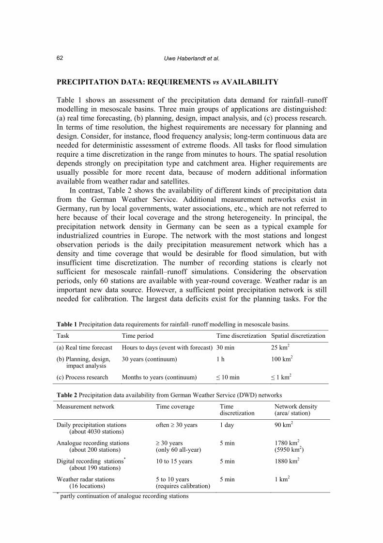
PRECIPITATION DATA: REQUIREMENTS vs AVAILABILITY Table 1 shows an assessment of the precipitation data demand for rainfall–runoff modelling in mesoscale basins. Three main groups of applications are distinguished: (a) real time forecasting, (b) planning, design, impact analysis, and (c) process research. In terms of time resolution, the highest requirements are necessary for planning and design. Consider, for instance, flood frequency analysis; long-term continuous data are needed for deterministic assessment of extreme floods. All tasks for flood simulation require a time discretization in the range from minutes to hours. The spatial resolution depends strongly on precipitation type and catchment area. Higher requirements are usually possible for more recent data, because of modern additional information available from weather radar and satellites. In contrast, Table 2 shows the availability of different kinds of precipitation data from the German Weather Service. Additional measurement networks exist in Germany, run by local governments, water associations, etc., which are not referred to here because of their local coverage and the strong heterogeneity. In principal, the precipitation network density in Germany can be seen as a typical example for industrialized countries in Europe. The network with the most stations and longest observation periods is the daily precipitation measurement network which has a density and time coverage that would be desirable for flood simulation, but with insufficient time discretization. The number of recording stations is clearly not sufficient for mesoscale rainfall–runoff simulations. Considering the observation periods, only 60 stations are available with year-round coverage. Weather radar is an important new data source. However, a sufficient point precipitation network is still needed for calibration. The largest data deficits exist for the planning tasks. For the Table 1 Precipitation data requirements for rainfall–runoff modelling in mesoscale basins.

Task Time period Time discretization Spatial discretization

(a) Real time forecast Hours to days (event with forecast) 30 min 25 km2

(b) Planning, design, impact analysis

30 years (continuum) 1 h 100 km2

(c) Process research Months to years (continuum) ≤ 10 min ≤ 1 km2 Table 2 Precipitation data availability from German Weather Service (DWD) networks

Measurement network Time coverage Time discretization

Network density (area/ station)

Daily precipitation stations (about 4030 stations)

often ≥ 30 years 1 day 90 km2

Analogue recording stations (about 200 stations)

≥ 30 years (only 60 all-year)

5 min 1780 km2

(5950 km2)

Digital recording stations*

(about 190 stations) 10 to 15 years 5 min 1880 km2

Weather radar stations (16 locations)

5 to 10 years (requires calibration)

5 min 1 km2

* partly continuation of analogue recording stations

Space–time representativity of precipitation for rainfall–runoff modelling

63

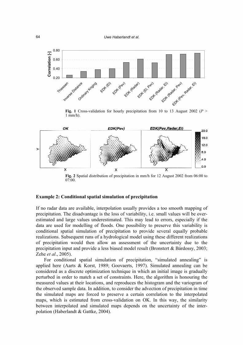
purpose of continuous rainfall–runoff simulations over periods of at least 30 years with a time resolution of 1 hour and a network density of one station per 100 km2, sufficient original precipitation data usually cannot be provided from the existing networks. A prerequisite for future improvement of the data situation is the continuous operation and possible extension of the precipitation measurement networks. However, for the solution of current tasks one has to manage with the available data. This requires on one hand, using all available information about precipitation (recording and non-recording stations, radar, weather prediction models, etc.) in an integrated way. On the other hand, stochastic simulation methods for synthesis, extension, and disaggregation can be applied. In the next sections examples for the improvement of the spatial and temporal representativity of precipitation are briefly discussed. IMPROVEMENT OF THE SPATIAL REPRESENTATIVITY Example 1: Optimal interpolation using additional information Quite a number of modern interpolation methods have been proposed for rainfall (Dubois et al., 1998). Often geostatistical approaches are utilised (Ehret, 2002; Goovaerts, 2000; Grimes et al., 1999; Seo et al., 1990a; Seo et al., 1990b). The first example discusses the optimal interpolation of hourly precipitation as an example for the heavy rainfall event of 10–13 August 2002 in parts of the Elbe River basin (Haberlandt, 2007). For interpolation, multivariate external drift kriging (EDK) using additional information from weather radar (Radar), daily precipitation in the form of the total event sum (Pev) and elevation (El) has been used. The main focus was on the optimal combination of point surface precipitation and weather radar data. The EDK method considers implicitly a space–time variable relationship between hourly point rainfall and all additional information, honouring the variability of the Z–R relationship. For the investigation, hourly precipitation from 21 recording stations, daily precipitation from 281 non-recording stations, and radar data from three locations were used. Figure 1 shows the results of a step-wise cross-validation for the interpolation of hourly precipitation using different methods with correlation as the performance criterion. The performance of the EDK approach is clearly better than for any univariate reference method. If no radar data are available, the best method is EDK using Pev as an additional variable. In this case, including elevation has no significant impact. However, when radar data are available elevation becomes significant and a model using Radar and El is recommended. This model is almost as good as the model using all three variables and has the advantage of being applicable for operational forecasts. Figure 2 shows the spatial distribution of precipitation for one selected hour of the event for the three interpolation methods, OK, EDK with the event sum Pev and EDK with Pev, Radar and El as additional variables. The application of OK based on the small sample size of 21 stations leads to very smooth maps. When using EDK with Pev more spatial structure becomes visible. The application of EDK with Radar, Pev and El as additional information improves the spatial representation of precipitation significantly. Those maps show more precipitation variability, higher extremes and the typical anisotropic rainfall patterns.


64

0.20

0.40

0.60

0.80

Thiess

en

Invers

e Dist

ance

Ordina

ry Krig

ing

EDK (El)

EDK (Pev

)

EDK (Rad

ar)

EDK (El, P

ev)

EDK (Rad

ar, E

l)

EDK (Rad

ar, P

ev)

EDK (Pev

, Rad

ar, E

l)

Cor

rela

tion

[-]

Fig. 1 Cross-validation for hourly precipitation from 10 to 13 August 2002 (P > 1 mm/h).

Fig. 2 Spatial distribution of precipitation in mm/h for 12 August 2002 from 06:00 to 07:00.

Example 2: Conditional spatial simulation of precipitation If no radar data are available, interpolation usually provides a too smooth mapping of precipitation. The disadvantage is the loss of variability, i.e. small values will be overestimated and large values underestimated. This may lead to errors, especially if the data are used for modelling of floods. One possibility to preserve this variability is conditional spatial simulation of precipitation to provide several equally probable realizations. Subsequent runs of a hydrological model using these different realizations of precipitation would then allow an assessment of the uncertainty due to the precipitation input and provide a less biased model result (Bronstert & Bárdossy, 2003; Zehe et al., 2005). For conditional spatial simulation of precipitation, “simulated annealing” is applied here (Aarts & Korst, 1989; Goovaerts, 1997). Simulated annealing can be considered as a discrete optimization technique in which an initial image is gradually perturbed in order to match a set of constraints. Here, the algorithm is honouring the measured values at their locations, and reproduces the histogram and the variogram of the observed sample data. In addition, to consider the advection of precipitation in time the simulated maps are forced to preserve a certain correlation to the interpolated maps, which is estimated from cross-validation on OK. In this way, the similarity between interpolated and simulated maps depends on the uncertainty of the inter-polation (Haberlandt & Gattke, 2004).


65

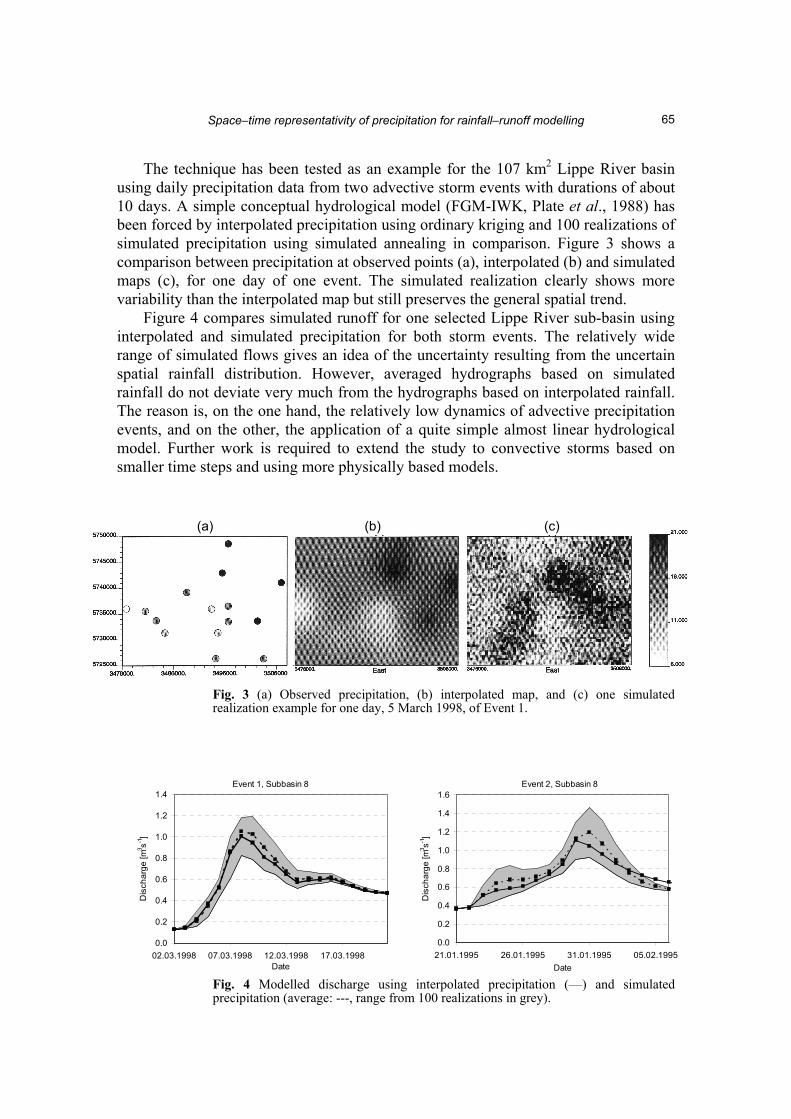
The technique has been tested as an example for the 107 km2 Lippe River basin using daily precipitation data from two advective storm events with durations of about 10 days. A simple conceptual hydrological model (FGM-IWK, Plate et al., 1988) has been forced by interpolated precipitation using ordinary kriging and 100 realizations of simulated precipitation using simulated annealing in comparison. Figure 3 shows a comparison between precipitation at observed points (a), interpolated (b) and simulated maps (c), for one day of one event. The simulated realization clearly shows more variability than the interpolated map but still preserves the general spatial trend. Figure 4 compares simulated runoff for one selected Lippe River sub-basin using interpolated and simulated precipitation for both storm events. The relatively wide range of simulated flows gives an idea of the uncertainty resulting from the uncertain spatial rainfall distribution. However, averaged hydrographs based on simulated rainfall do not deviate very much from the hydrographs based on interpolated rainfall. The reason is, on the one hand, the relatively low dynamics of advective precipitation events, and on the other, the application of a quite simple almost linear hydrological model. Further work is required to extend the study to convective storms based on smaller time steps and using more physically based models.

Fig. 3 (a) Observed precipitation, (b) interpolated map, and (c) one simulated realization example for one day, 5 March 1998, of Event 1.

Event 1, Subbasin 8

0.0

0.2

0.4

0.6

0.8

1.0

1.2

1.4

02.03.1998 07.03.1998 12.03.1998 17.03.1998Date

Dis

char

ge [m

3 s-1]

Event 2, Subbasin 8

0.0

0.2

0.4

0.6

0.8

1.0

1.2

1.4

1.6

21.01.1995 26.01.1995 31.01.1995 05.02.1995Date

Dis

char

ge [m

3 s-1]

Fig. 4 Modelled discharge using interpolated precipitation (—) and simulated precipitation (average: ---, range from 100 realizations in grey).

(a) (b) (c)


66

IMPROVEMENT OF THE REPRESENTATIVITY IN TIME Example 3: Stochastic synthesis of hourly precipitation For derived flood frequency analysis of extreme flows based on hydrological model-ling, long continuous precipitation time series are needed. Often, the observed precipitation time series are too short, so stochastic precipitation synthesis is required. Over recent years, several stochastic precipitation models for short-term rainfall have been proposed (e.g. Acreman, 1990; Cowpertwait, 2006; Pegram & Clothier, 2001; Rodriguez-Iturbe et al., 1987; Wheater et al., 2005). This example presents a simple stochastic precipitation model which divides the generation process into two stages. First, a classical alternating renewal model (Haberlandt, 1998) is adapted and then applied to simulate independent precipitation time series for several locations. In the second step, a resampling procedure will be used (similar to, e.g. Bárdossy, 1998) to reproduce the spatial dependence structure and further characteristics such as season-ality. In the following, only the first stage of the precipitation generation process will be reported. The model was developed for precipitation synthesis in the 3200 km2 Bode River basin located in the Harz Mountains in northern Germany. Data are available from about 20 recording raingauges in the greater region of the basin. Alternating Renewal Models describe the precipitation process by dividing the time series into dry and wet spells. The entire precipitation process is separated into an external and an internal structure. The external structure characterizes the occurrence and the amount of the precipitation events, as explained by the variables dry-spell-duration (dsd), wet-spell-duration (wsd) and wet-spell-amount (wsa). The internal structure describes the precipitation distribution within the wet-spells (see Fig. 5). The precipitation occurrence process is completely determined by establishing probability distributions for the variables dsd and wsd. A basic condition is the independence and identical distribution of the durations of the wet and dry spells. However, wsa cannot be treated as independent of wsd. Wet- and dry-spell durations are modelled here by the Weibull and general extreme value distributions, respectively. Wet spell amounts are modelled using a Weibull distribution. The dependence between wet spell amount and duration is described by a 2D copula (see, e.g. De Michele & Salvadori, 2003). For disaggregation of the wet spells in to hourly intensities, a special profile with random

dsd1 dsd2

wet-spell- dry-spell

entire eventPi

Timewsd1 wsd2 wsd3

wsi1

dsd1 dsd2dsd1 dsd2


entire event


entire eventPi

Time

Pi

Timewsd1 wsd2 wsd3wsd1 wsd2 wsd3

wsi1wsi1

Fig. 5 Scheme of the precipitation event process (P: precipitation; wsi: wet spell intensity; wsd: wet spell duration; dsd: dry spell duration).


67

Table 3 Precipitation event statistics for the Harzgerode station (1993–2004).

Mean: Number (-)

Volume (mm)

StdDev (mm)

Skewness (-)

Annual precipitation (mm)

Observed 163 3.48 5.28 6.10 568

Simulated 160 3.49 5.06 4.46 559

0

10

20

30

40

50

0 0.2 0.4 0.6 0.8 1

Non-exceedance Prob. [-]

Prec

ipita

tion

[mm

]

SimulatedObserved

Fig. 6 Empirical distribution of annual maximum observed (12 year) and eight realizations of simulated (8 × 12 year) hourly precipitation for the 1 hour duration class of the Harzgerode station.

peak time is used (Haberlandt, 1998). Table 3 presents some basic statistical event characteristics from observed and simulated precipitation for the Harzgerode station, demonstrating quite good performance. Also, the reproduction of extreme values is satisfactory, as shown in Fig. 6. The results demonstrate that univariate simulation of hourly precipitation is possible using a simple model with good performance. The main challenge is the simulation of the space–time structure while keeping the model as simple as possible, which is currently being investigated and will be reported elsewhere. Example 4: Disaggregation of daily precipitation Usually the availability of daily precipitation data is much better than for hourly data (see Table 2). Thus one interesting alternative is the disaggregation of daily rainfall into smaller time steps (Gyasi-Agyei, 2005; Lovejoy & Schertzer, 2006; Olsson, 1998). The disaggregated data still have a real-time relation, which is an advantage compared to pure stochastic simulation. The disadvantage is the restriction to the observed time period, which might be too short for the estimation of extreme values. For disaggregation, a multiplicative random cascade model with exact mass conservation is applied here (Güntner et al., 2001). The model divides the observed 24-hour precipitation into two equal-size non-overlapping boxes having one of the three possible states with certain transition probabilities: wet/wet with P(x/1 – x),


68

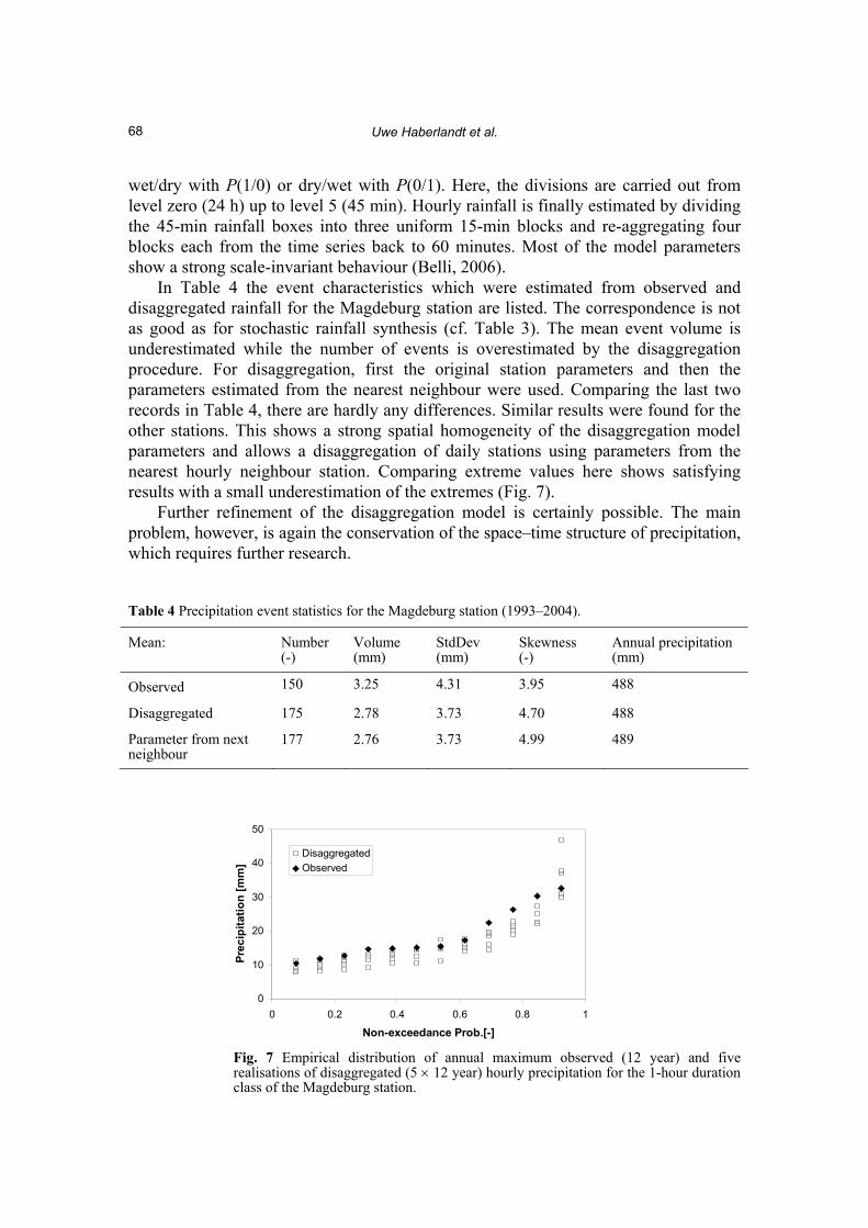
wet/dry with P(1/0) or dry/wet with P(0/1). Here, the divisions are carried out from level zero (24 h) up to level 5 (45 min). Hourly rainfall is finally estimated by dividing the 45-min rainfall boxes into three uniform 15-min blocks and re-aggregating four blocks each from the time series back to 60 minutes. Most of the model parameters show a strong scale-invariant behaviour (Belli, 2006). In Table 4 the event characteristics which were estimated from observed and disaggregated rainfall for the Magdeburg station are listed. The correspondence is not as good as for stochastic rainfall synthesis (cf. Table 3). The mean event volume is underestimated while the number of events is overestimated by the disaggregation procedure. For disaggregation, first the original station parameters and then the parameters estimated from the nearest neighbour were used. Comparing the last two records in Table 4, there are hardly any differences. Similar results were found for the other stations. This shows a strong spatial homogeneity of the disaggregation model parameters and allows a disaggregation of daily stations using parameters from the nearest hourly neighbour station. Comparing extreme values here shows satisfying results with a small underestimation of the extremes (Fig. 7). Further refinement of the disaggregation model is certainly possible. The main problem, however, is again the conservation of the space–time structure of precipitation, which requires further research. Table 4 Precipitation event statistics for the Magdeburg station (1993–2004).

Mean: Number (-)

Volume (mm)

StdDev (mm)

Skewness (-)

Annual precipitation (mm)

Observed 150 3.25 4.31 3.95 488

Disaggregated 175 2.78 3.73 4.70 488

Parameter from next neighbour

177 2.76 3.73 4.99 489

0

10

20

30

40

50

0 0.2 0.4 0.6 0.8 1

Non-exceedance Prob.[-]

Prec

ipita

tion

[mm

]

DisaggregatedObserved

Fig. 7 Empirical distribution of annual maximum observed (12 year) and five realisations of disaggregated (5 × 12 year) hourly precipitation for the 1-hour duration class of the Magdeburg station.


69

CONCLUSIONS The following points summarize the results: (a) The largest short-coming of precipitation data is the lack of continuous long-term

short-time-step series for rainfall–runoff simulations for planning and design. (b) All available information about precipitation (e.g. non-recording and recording

point gauges, radar, etc.) should be used together for rainfall–runoff modelling. (c) There are several simple reliable time rainfall models available which should be

utilised more frequently as input data generators for hydrological modelling. (d) Research is still required for the development of simple parsimonious space–time

models of rainfall with satisfactory performance.

REFERENCES

Aarts, E. & Korst, J. (1989) Simulated Annealing and Boltzmann Machines. John Wiley, New York, USA. Acreman, M. C. (1990) Simple stochastic model of hourly rainfall for Farnborough, England. Hydrol. Sci. J. 35(2), 119–148. Bárdossy, A. (1998) Generating precipitation time series using simulated annealing. Water Resour. Res. 34(7), 1737–1744. Belli, A. (2006) Untersuchungen zur zeitlichen Disaggregation kontinuierlicher Niederschlagszeitreihen. Studienarbeit

Thesis, Inst. für Wasserwirtschaft, Leibniz Universität Hannover, Germany. Bronstert, A. & Bárdossy, A. (2003) Uncertainty of runoff modeling at the hillslope scale due to temporal variations of

rainfall intensity. Physics & Chemistry of the Earth 28, 283–288. Cowpertwait, P. S. P. (2006) A spatial-temporal point process model of rainfall for the Thames catchment, UK. J. Hydrol.

330(3-4), 586–595. De Michele, C. & Salvadori, G. (2003) A Generalized Pareto intensity–duration model of storm rainfall exploiting

2-copulas. J. Geophys. Res. 108(D2), 4067, doi:10.1029/2002JD002534. Dubois, G., Malczewski, J. & Cort, M. D. (eds) (1998) Spatial Interpolation Comparison 97. Special issue: J. Geogr.

Information and Decision Analysis 2(1–2). Ehret, U. (2002) Rainfall and flood nowcasting in small catchments using weather radar. Dissertation, Mitteilungen des

Instituts für Wasserbau, Heft 21, Stuttgart, Germany. Goovaerts, P. (1997) Geostatistics for Natural Resources Evaluation. Oxford University Press, Oxford, UK. Goovaerts, P. (2000) Geostatistical approaches for incorporating elevation into the spatial interpolation of rainfall.

J. Hydrol. 228(1-2), 113–129. Grimes, D. I. F., Pardo-Iguzquiza, E. & Bonifacio, R. (1999) Optimal areal rainfall estimation using raingauges and

satellite data. J. Hydrol. 222, 93–108. Güntner, A., Olsson, J., Calver, A. & Gannon, B. (2001) Cascade-based disaggregation of continuous rainfall time series:

the influence of climate. Hydrol. Earth System Sci. 5, 145–164. Gyasi-Agyei, Y. (2005) Stochastic disaggregation of daily rainfall into one-hour time scale. J. Hydrol. 309(1-4), 178–190. Haberlandt, U. (1998) Stochastic rainfall synthesis using regionalized model parameters. J. Hydrol. Engng 3(3), 160–168. Haberlandt, U. (2007) Geostatistical interpolation of hourly precipitation from rain gauges and radar for a large-scale

extreme rainfall event. J. Hydrol. 332, 144–157. Haberlandt, U. & Gattke, C. (2004) Spatial interpolation vs. simulation of precipitation for rainfall-runoff modelling - a

case study in the Lippe River basin. In: Hydrology Science and Practice for the 21st Century, vol. 1, 120–127. British Hydrological Society, London, UK.

Lovejoy, S. & Schertzer, D. (2006) Multifractals, cloud radiances and rain. J. Hydrol. 322(1-4), 59–88. Olsson, J. (1998) Evaluation of a scaling cascade model for temporal rainfall disaggregation. Hydrol. Earth System Sci. 2, 19–30. Pegram, G. G. S. & Clothier, A. N. (2001) High resolution space–time modelling of rainfall: the "String of Beads" model.

J. Hydrol. 241(1-2), 26–41. Plate, E. J., Ihringer, J. & Lutz, W. (1988) Operational models for flood calculations. J. Hydrol. 100, 489–506. Rodriguez-Iturbe, I., Cox, D. R. & Isham, V. (1987) Some models for rainfall based on stochastic point processes. Proc.

Royal Soc. London A 410, 269–288. Seo, D.-J., Krajewski, W. F. & Bowles, D. S. (1990a) Stochastic interpolation of rainfall data from raingages and radar

using co-kriging: 1. Design of experiments. Water Resour. Res. 26(3), 469–477 (89WR02984). Seo, D.-J., Krajewski, W. F. & Bowles, D. S. (1990b) Stochastic interpolation of rainfall data from raingages and radar

using co-kriging: 2. Results. Water Resour. Res. 26(5), 915–924 (89WR02992). Wheater, H., et al. (2005) Spatial-temporal rainfall modelling for flood risk estimation. Stoch. Environ. Res. Risk Assess.

(SERRA) 19(6), 403–416. Zehe, E., Becker, R., Bardossy, A. & Plate, E. (2005) Uncertainty of simulated catchment runoff response in the presence

of threshold processes: role of initial soil moisture and precipitation. J. Hydrol. 315(1-4), 183–202.

space–time representativity of precipitation for rainfall

Documents