space weather impact on ground-based technological systems
TRANSCRIPT
Solar-Terrestrial Physics. 2021. Vol. 7. Iss. 3. P. 68–104. DOI: 10.12737/stp-73202106. © 2021 Pilipenko V.A. Published by INFRA-M Academic Publishing House. Original Russian version: Pilipenko V.A., published in Solnechno-zemnaya fizika.
2021. Vol. 7. Iss. 3. P. 72–110. DOI: 10.12737/szf-73202106. © 2021 INFRA-M Academic Publishing House (Nauchno-Izdatelskii Tsentr INFRA-M)
This is an open access article under the CC BY-NC-ND license
SPACE WEATHER IMPACT ON GROUND-BASED TECHNOLOGICAL SYSTEMS
V.A. Pilipenko Institute of Physics of Earth RAS,
Moscow, Russia, [email protected]
Geophysical Center RAS,
Moscow, Russia, [email protected]
Abstract. This review, offered for the first time in
the Russian scientific literature, is devoted to various
aspects of the problem of the space weather impact on
ground-based technological systems. Particular attention
is paid to hazards to operation of power transmission
lines, railway automation, and pipelines caused by geo-
magnetically induced currents (GIC) during geomagnet-
ic disturbances. The review provides information on the
main characteristics of geomagnetic field variability, on
rapid field variations during various space weather man-
ifestations. The fundamentals of modeling geoelectric
field disturbances based on magnetotelluric sounding
algorithms are presented. The approaches to the assess-
ment of possible extreme values of GIC are considered.
Information about economic effects of space weather
and GIC is collected. The current state and prospects of
space weather forecasting, risk assessment for techno-
logical systems from GIC impact are discussed. While
in space geophysics various models for predicting the
intensity of magnetic storms and their related geomag-
netic disturbances from observations of the interplane-
tary medium are being actively developed, these models
cannot be directly used to predict the intensity and posi-
tion of GIC since the description of the geomagnetic
field variability requires the development of additional
models. Revealing the fine structure of fast geomagnetic
variations during storms and substorms and their in-
duced GIC bursts appeared to be important not only
from a practical point of view, but also for the develop-
ment of fundamentals of near-Earth space dynamics.
Unlike highly specialized papers on geophysical aspects
of geomagnetic variations and engineering aspects of
the GIC impact on operation of industrial transformers,
the review is designed for a wider scientific and tech-
nical audience without sacrificing the scientific level of
presentation. In other words, the geophysical part of the
review is written for engineers, and the engineering part
is written for geophysicists. Despite the evident applied
orientation of the studies under consideration, they are
not limited to purely engineering application of space
geophysics results to the calculation of possible risks for
technological systems, but also pose a number of fun-
damental scientific problems.
Keywords: space weather, geomagnetically induced currents, power transmission lines, transformers, pipe-lines, railways automation, magnetospheric storms, sub-storms, Pi3/Ps6 pulsations.
CONTENT
1 Negative impact of space weather on technological systems………………………………………….. 69
1.1 Power grids……………………………………………………………………………………………… 69
1.2 Cable lines, telephone and telegraph lines……………………………………………………………… 70
1.3 Railway equipment…………………………………………………………………………………….... 70
1.4 Pipelines…………………………………………………………………………………………………. 71
2 Geomagnetic and geoelectric field variations during various space weather manifestations………….. 71
2.1 Interplanetary shock waves…………………………………………………………………………….... 72
2.2 Auroral and polar substorms…………………………………………………………………………….. 72
2.3 Local pulse disturbances of the geomagnetic field……………………………………………………… 73
2.4 Substorm fine structure: series of Ps6/Pi3 magnetic pulses……………………………………………. 74
2.5 Pc5 pulsations………………………………………………………………………………………….... 74
2.6 Statistical features of geomagnetic field variability dB/dt……………………………………………… 75
3 Failures in technological systems caused by GIC……………………………………………………..... 77
3.1 Malfunctions in the operation of industrial transformers at auroral latitudes ……………..................... 77
3.2. GIC at middle and low latitudes……………………………………………………………………….... 78
3.3. Failures in the operation of railway equipment………………………………………………................ 78
3.4 Pipelines…………………………………………………………………………………………………. 79
4 GIC measurement methods……………………………………………………………………………… 80
4.1 Power transmission line Nord Transit…………………………………………………………………... 80
4.2 Differential magnetometry method……………………………………………………………………… 80
4.3 Power grid harmonics………………………………………………………………………………….... 81
4.4 GIC in power grids and VLF radio emission…………………………………………………………… 82
V.A. Pilipenko
69
5 Modeling geoelectric field disturbances and GIC…………………………………………………….... 82
5.1 MT-sounding methods…………………………………………………………………………………... 82
5.2 Variations in geomagnetic and telluric fields as a source of GIC……………………………………… 83
5.3 Maps of possible GIC values……………………………………………………………………………. 83
5.4 Transfer function method for assessing GIC in given systems during geomagnetic varia-tions……………………………………………………………………………………………
85
5.5 Models for calculating pipeline GIC and the pipe-to-soil potential…………………………………….. 85
5.6. Influence of sharp irregularities of geoelectric conductivity on GIC…………………………………..... 86
6 Estimated possible extreme GIC values…………………………………………………………………… 86
6.1 Statistical methods for estimating extreme events……………………………………………………….. 87
6.2 Estimated extreme values of variability in geomagnetic field and telluric fields……………………….. 87
7 РС index of geomagnetic activity and failures in power grids…………………………………………… 87
8 Economic effects of GIC………………………………………………………………………………….. 88
9 GIC in conductive systems and power transformers……………………………………………………… 89
10 Development of physical and statistical models for assessing the risk from negative GIC effects 90
10.1 Statistical relationships between variations in the geomagnetic field, auroral electrojet, and geomagnetically induced currents…………………………………………………………………………………………..
90
10.2 Regression model of geomagnetically induced currents………………………………………………… 91
10.3 Statistical distributions of GIC and geomagnetic variations……………………………………………. 92
11 Forecast of space weather, auroral oval position, and risk for power grids with global MHD simula-tion……………………………………………………………………………………………………...
92
11.1 Computer models of real-time forecast of GIC risks……………………………………………………. 94
11.2 Predictive models of auroral oval intensity and position……………………………………………….. 95
12 Conclusion: Objectives of further research……………………………………………………………... 96
1. NEGATIVE IMPACT
OF SPACE WEATHER
ON TECHNOLOGICAL SYSTEMS
Research into the state of near-Earth space, called
space weather (SW) for short, i.e. the state of electro-
magnetic fields, plasma, and particle fluxes in near-
Earth space (NES), extends beyond purely academic
interest as the number of problems associated with
failures in satellite-borne and ground-based technolog-
ical systems increases [Space Weather — Research
Towards Applications in Europe, 2007]. Among these
problems are failures in satellite and aviation systems,
partial or total power outages, failures in signals from
global navigation satellite systems (GPS, GLONASS),
interference in radio communications [Space Storms
and Space Weather Hazards, 2000; Extreme Space
Weather: Impacts on Engineered Systems and Infra-
structure, 2013]. The most active SW effects such as
disturbances of the geomagnetic field and the iono-
sphere, excitation of geomagnetically induced currents
(GICs) in conducting structures, failures in radio
communications and navigation satellite systems, in-
creasing corrosion in pipelines, etc. are observed at
high latitudes [Space Weather, 2001].
At the same time, the more widely advanced techno-
logical systems are introduced, the more sensitive their
failures and outages become for economy and life activ-
ity of mankind. Expansion of trunk power transmission
lines (PTL) is accompanied by an increase in the occur-
rence rate of failures caused by GIC driven by geomag-
netic storms and substorms [Boteler, 2001]. There are
numerous examples of devastating impacts of SW
events all over the world [Lanzerotti, 1979, 1983, 2001 ;
Bolduc, 2002]. Variability of SW factors and their nega-
tive impact on the technological environment are a natu-
ral norm that cannot be avoided, but must be known and
taken into account [Pirjola et al., 2005]. When address-
ing engineering problems, it is necessary to know SW
characteristic parameters and the range of their varia-
tions in order to improve existing technical facilities and
to properly develop new ones [Veeramany et al., 2016].
Space weather is generally determined by solar
flares, coronal mass ejections, and high-speed plasma
fluxes from solar holes (corotating interaction regions),
which trigger geomagnetic storms and substorms. The
total amount of energy released by a medium intensity
magnetic storm is ~1400 GW, which is almost double the
capacity of all power plants in the United States. Extensive
research on SW problems undertaken in the world is, on
the one hand, defined by the fundamental scientific interest
in the problem of studying solar-terrestrial relations and
geophysical shells as a single dynamic system; on the other
hand, by the need to ensure the stable operation of techno-
logical systems, radio communications, radar, and naviga-
tion.
1.1. Power grids
The frequency of solar plasma ejections into inter-
planetary space increases during solar maximum, but
does not stop during solar minimum. The solar plasma
ejections flying by Earth deform its protective magnetic
field, causing amplification of electromagnetic fields
Space weather impact on ground-based technological systems
70
both in near space and near Earth's surface [Love,
2008]. Variations in geoelectric currents induced in sur-
face layers of the earth's crust are completed through
grounded power systems, giving rise to GIC [Boteler,
Pirjola, 2017, 2019]. In turn, GIC lead to voltage drops,
overheating of power transformers, and loss of reactive
power in high-voltage PTL [Pirjola, 1985a, b; Uspen-
sky, 2017; Vakhnina et al., 2018]. To date, GIC have
become a constant hazard for high-technology societies,
posing a grave danger to regional high-voltage electric
power networks, many of which cross national bounda-
ries [Gaunt, 2016].
Modern power grids with extremely complex geom-
etry, located up to high latitudes, are in fact a giant an-
tenna, electromagnetically coupled with currents of
Earth's ionosphere [Piccinelli, Krausmann, 2014]. In
grounded power grids, currents up to 300 A were ob-
served, while GIC with an intensity of only a few am-
peres is sufficient to affect the operation of a transform-
er [Overbye et al., 2013]. Although geomagnetic and
ionospheric disturbances leading to excitation of GIC in
conducting structures occur generally at auroral high
latitudes [Myllys et al., 2014], it has recently been found
that dangerous GIC values can be seen at middle and
even low latitudes [Beggan et al., 2013].
Calculating possible GIC levels during typical and
extreme magnetic storms, which can be used by net-
work operators to take the necessary measures to reduce
the risk of catastrophic consequences, is the most press-
ing challenge [Sokolova et al., 2021]. Solving the prob-
lems of minimizing the risk of occurrence and reducing
the consequences of natural disasters requires clarifying
the physical nature of some magnetospheric-ionospheric
phenomena, and not just be limited to the engineering
application of results of space physics to calculation of
GIC in technological systems [Pulkkinen et al., 2017].
On the one hand, there is a need for a global planetary
approach to the description of geomagnetic disturb-
ances; on the other hand, to study GIC in each specific
system [Hapgood, 2012; Viljanen, Tanskanen, 2011;
Viljanen et al., 2013].
During industrial development, the length and inter-
connectedness of power lines sharply increase, which
makes them more sensitive to the negative impact of
GIC. In order to transmit a large amount of electric
power over long distances, more and more extended
power transmission lines are being built. However, such
lines are especially affected by strong GIC. This cir-
cumstance makes electrical networks more and more
susceptible to SW disturbances. For example, in Canada
and the United States, GIC levels have become 2–3
times higher than those observed 20 years ago during
magnetic storms of the same intensity [Molinski, 2002].
Moreover, failures in power grids can be caused not
only by extreme SW disturbances, but also by prema-
ture aging of components of high-voltage transformers
due to the cumulative effect of even moderate GIC,
which are generally considered to be no-damage [Bé-
land, Small, 2005]. The GIC impact can also be affected
by network loading. For example, Wik et al. [2009]
have shown that the July 13–14, 1982 magnetic storm
would have had serious consequences but for favorable
conditions in the power grid due to the low summer
load.
Failures in PTL are the most obvious but not the on-
ly consequence of GIC. Unbalanced transformers with
partially saturated cores increase the reactance and the
content of harmonics of supplied power from electric
power stations [Arrillaga et al., 1990]. Consequently,
the efficiency of power distribution decreases, which
may lead to a decrease in the power available to con-
sumers. In extreme cases, electric power networks can
become unstable and fail, causing large-scale power
outages.
There are many examples of serious consequences
of the SW impact on long-distance high-voltage elec-
tric power networks [Bozoki, 1996; Qiu et al., 2015].
GIC caused saturation, an increase in harmonics, over-
heating, and even damage to high-voltage transform-
ers. The most intense currents (more than a hundred of
A) were measured in neutral terminals of transformers
at auroral latitudes during magnetic storms and sub-
storms [Viljanen et al., 2014]. There is, however, no
general rule on how strong GIC should be to pose a
hazard to power grids as there are many types of trans-
formers with different sensitivity to quasi-DC currents.
Some power transformers require only a few amperes
to be taken out of the linear mode [Vakhnina, 2012;
Vakhnina et al., 2012; Vakhnina, Kretov, 2012a].
The constant expansion of high-voltage power net-
works, an increase in the connection between them,
growth of the load, and transition to low-resistance
power lines with a higher voltage lead to an increase in
the probability of accidents during SW disturbances.
However, catastrophic failures are not necessary to have
a tangible economic impact on the functioning of
wholesale electricity markets. Therefore, even if equip-
ment for energy infrastructure is not destroyed during
strong SW disturbances, GIC in regional power systems
can still have a noticeable effect on the economy as a
whole [Forbes, 2004].
1.2. Cable lines, telephone and telegraph lines
Through GIC, SW reveals itself in the operation of oth-
er technological systems — telegraph lines, submarine
cables [Lanzerotti et al., 1995]. More than a century ago,
the magnetic storm on June 17, 1915 disrupted telegraph
services throughout most of the world. The GIC hazard to
trunk and marine cable lines, telephone and telegraph lines
was repeatedly confirmed later on [Anderson et al., 1974;
Medford et al., 1981; Meloni et al., 1983; Boteler, Jansen
van Beek, 1999].
1.3. Railway equipment
While in most of SW studies prominence is given to the impact on power networks, disruptions to the rail-way sector receive much less attention. Anomalies in train signaling and control systems associated with this phenomenon have, however, been documented [Liu et al., 2016; Eroshenko et al., 2010; Sakharov, et al., 2009]. Nonetheless, the mechanism of the impact of strong ge-omagnetic disturbances on the operation of railway au-
V.A. Pilipenko
71
tomation systems has not yet been clarified [Trishchenko, 2008]. Furthermore, railway systems rely on other po-tentially SW-affected technologies such as power sup-ply, communications, positioning and time synchroniza-tion systems. Since during strong storms the impact of the disturbances is quite widespread and global, it is necessary to predict SW events and develop measures to reduce direct and indirect impacts of the disturbances on railway systems and services [Krausmann et al., 2015].
1.4. Pipelines
Space weather and related global electromagnetic
disturbances pose a hazard to pipelines, especially those
located in the zone of intense geomagnetic activity
[Pulkkinen et al., 2001a, b; Gummow, Eng, 2002]. The
effects of geomagnetic disturbances on pipelines are not
instantaneous, but have a cumulative effect due to sus-
ceptibility to corrosion [Boteler, Cookson, 1986; Mar-
tin, 1993; Boteler, Trichtenko, 2015; Marshall et al.,
2010]. Electrocorrosion is an electrochemical process
that occurs when current flows from the pipe into the
soil. To prevent corrosion, steel pipelines are covered
with an insulating coating and equipped with a cathodic
protection system. Cathodic protection of pipelines from
electrocorrosion maintains a negative potential of the
order of –1 V with respect to the ground. During a mag-
netic storm in November 2004 on a gas pipeline in Fin-
land, the pipe-to-soil potential ranged from 1.6 V to 4 V
[Pirjola et al., 2003].
Under the GIC impact, the cathodic protection of pipelines, which maintains the negative potential of the pipe with respect to the ground, is distorted, thereby increasing sharply the corrosion rate and reducing the service life of pipelines. High-frequency (50–60 Hz) electric fields in pipelines can also be induced by nearby power transmission lines. To protect against GIC, pipe-lines are divided into shorter sections with insulating inserts. This reduces the extreme potential values be-tween the pipe and the ground, but increases the number of non-zero potential sections, which increases the risk of corrosion.
The fundamental difference between pipelines and PTL is that the former are grounded continuously. A pipeline that is grounded at many points actually shunts the electric field induced on the surface. The electric field component parallel to a pipeline can induce cur-rents in it up to 100 A [Viljanen et al., 2006b]. Near pipe ends, pumping stations, at junctions of pipes of different diameters, as the direction of the pipe is changed, the distribution of ground currents changes, the pipe-to-soil potential is redistributed, which can sig-nificantly affect the corrosion rate and the cathodic pro-tection. Similar effects can also occur in places of local changes in ground conductivity [Viljanen, 1989; Sack-inger, 1991; Fernberg et al., 2007], as well as when a pipeline moves from the ground to the sea. For pipelines located on the seabed (Nord Stream-2 type), the envi-ronment is well-conductive seawater. In such systems, GIC have not been detected; however, the GIC impact is to be expected in this case too.
Thus, the influence of geomagnetic variations should be taken into account when designing pipelines, choos-
ing and organizing a cathodic protection system [Hen-riksen et al., 1978; Lundstend, 1992]. Since the GIC impact can appear both directly during the development of a disturbance and be cumulative, it is advisable to organize a system for continuous monitoring of GIC level and pipe-to-soil potentials at a number of interme-diate stations and a system for continuous recording of magnetic variations. Information on the response of individual pipeline sections to magnetic disturbances during the operation of a pipeline will make it possible to choose optimal ground and cathodic protection cir-cuits. To assess the degree of influence of geomagnetic and geoelectric fields on a specific system, it is wise to draw up a map of the probability of deviations of fields from a quiet level [Trichtchenko, Boteler, 2002]. Since in Russia the length of existing pipelines connecting the Arctic regions with midlatitudes is quite considerable, the problem of the negative GIC impact on pipelines deserves special attention.
2. GEOMAGNETIC AND GEOELECTRIC FIELD
VARIATIONS DURING VARIOUS SPACE WEATHER MANIFESTATIONS
One of the most significant SW factors is the electri-cal GIC in technological conductor systems, which is associated with abrupt changes in the geomagnetic field dB/dt [Knipp, 2015]. The most considerable magnetic disturbances on Earth's surface are caused by an extend-ed auroral electrojet, which generates magnetic disturb-ances oriented in the latitudinal (NS) direction on Earth's surface. There are, therefore, widespread con-cepts and computational models in which the main source of GIC is the auroral electrojet intensity varia-tions producing GIC in the longitudinal (EW) direction [Hakkinen, Pirjola, 1986; Viljanen, Pirjola, 1994; Botel-er, Pirjola, 1998; Boteler et al., 2000]. Based on this fact, it was believed that magnetic disturbances pose a hazard mainly to the technological systems extended in the longitudinal direction [Pirjola, 1982].
Small-scale ionospheric current structures can none-theless make a significant contribution to the rapid changes in the magnetic field, which are essential for the excitation of GIC [Viljanen, 1997; Viljanen et al., 2001]. They create almost isotropic disturbances of hor-izontal magnetic fields on Earth's surface. Data on the excitation and development of GIC in real conducting systems is of fundamental interest in terms of the fine structure of the development of disturbances and is of practical importance in terms of protecting technologi-cal systems from the SW impact.
Specific examples of SW disturbances of various
types able to induce high-intensity currents in power
transmission lines are given below. Analysis of individ-
ual events shows that the amplification of a large-scale
auroral electrojet during the substorm expansion phase,
Pi3/Ps6 and Pc5 geomagnetic pulsations, daytime sud-
den impulses, and nighttime sporadic magnetic impulses
can lead to significant increases in GIC. Energy of such
impulsive or quasiperiodic disturbances is much lower

Space weather impact on ground-based technological systems
72
than that of magnetospheric storms or substorms; yet
rapidly changing fields of such disturbances can cause
GIC bursts of great intensity. In general, amplitudes of
geomagnetic variations decrease with frequency, where-
as induced electric field intensities are expected to in-
crease with frequency. Accordingly, the GIC response
to a geomagnetic disturbance, which is a combination of
both factors, should have a maximum at some frequen-
cies. Studies of GIC bursts have shown that this charac-
teristic time scale is ~2–10 min, i.e. it falls into the fre-
quency range of Pc5/Pi3 pulsations, being in the low-
frequency interval of the ultra-low-frequency (ULF)
band.
2.1. Interplanetary shock waves
Among the wide variety of MHD disturbances in
NES, particular emphasis is given to the study of the
storm sudden commencement (SSC), caused by the in-
teraction of the interplanetary shock wave with the
magnetosphere. The impulse action of the shock wave
can bring a significant amount of energy and momen-
tum into the magnetosphere for a very short period of
time. Pulse SSC disturbances are precursors of strong
geomagnetic storms. The shock action on the geomag-
netic field has an important practical aspect as a source
of GIC [Belakhovsky et al., 2017]. The GIC effect on
power systems was observed at dB/dt>100 nT/min
[Kappenman, 1996]. Some power system failures were
associated with the occurrence of SSC even before the
onset of the magnetic storm main phase [Zhang et al.,
2015]. For example, the destruction of the power grid
transformer in New Zealand [Béland, Small, 2005] co-
incided with SSC. While the SSC associated disturbance
B is rather weak as compared to B during the storm
or substorm main phase, dB/dt can be great enough to
induce hazardous GIC in power grids. At the same time,
the magnetic field variation dB/dt during SSC is not
unambiguously related to the intensity of the subsequent
magnetic storm [Fiori et al., 2014].
Due to the global nature of the interplanetary shock
wave action on the geomagnetic field, dB/dt at the equa-
tor may be comparable to the levels in high-latitude
regions [Carter et al., 2015]. At near-equatorial lati-
tudes, the influence of the equatorial electrojet may turn
out to be significant for the development of induction
effects. During SSC on February 17, 1993, peak values
of the geoelectric field were as high as 300 mV/km at a
geomagnetic latitude of ~5° [Doumbia et al., 2017].
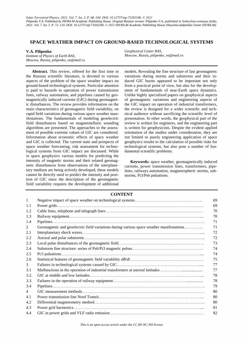
A typical example is the burst in the system for GIC
detection in power transmission lines on the Kola Pen-
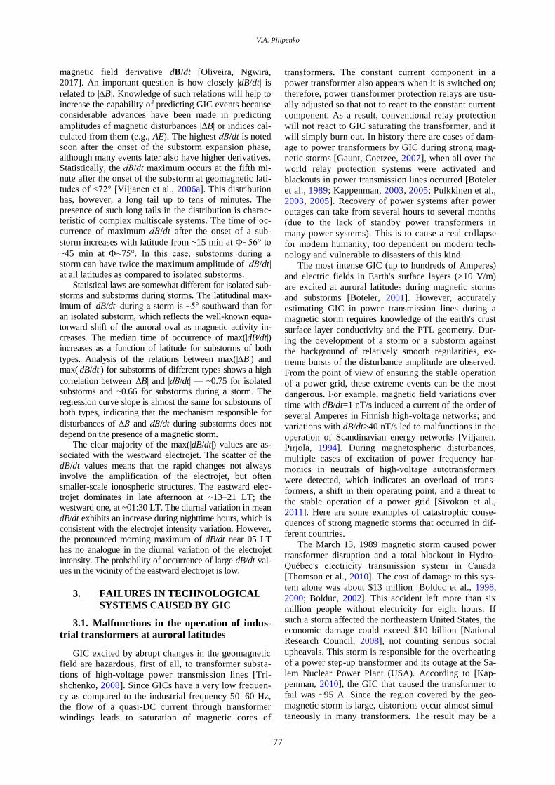
insula during SSC on March 17, 2015 (Figure 1) [Pili-
penko et al., 2018a]. At the moment of the interplane-
tary shock wave action on Earth's magnetosphere, which
appeared on Earth's surface as an SSC pulse at ~06 UT,
a sudden burst of GIC occurred at stations of the Nord
Transit system. Variations in GIC at VKH are similar to
those in the derivative of the magnetic field dX/dt at the
nearby magnetic station IVA (~10 nT/s). The amplitude
of SSC driven GIC variations (~55 A) is approximately
two times higher than that of GIC (<30 A) during subse-
Figure 1. Variations in the magnetic field (X compo-
nent) at IVA, derivative of dX/dt; the same for the Y com-
ponent; GIC values at the VKH substation during the
March 17, 2015 magnetic storm
quent intensifications of the substorm, although the SSC
amplitude (~200 nT) is lower than that of the magnetic
bay associated with the substorm (~1000 nT). This is
consistent with a higher amplitude of dX/dt during SSC
compared to that observed during the intensification of
the substorm at ~13 UT and ~17 UT.
Thus, such an SW phenomenon as SSC can produce
very high dB/dt at latitudes from the auroral region to
the geomagnetic equator. For PTL operators, SSC ap-
pears as a short circuit in the line. The SSC impact may
be a significant factor affecting stability of power
transmission.
2.2. Auroral and polar substorms
Unlike planetary disturbances such as magnetic
storms, substorms develop only in the nightside magne-
tosphere. During one typical 11-year solar cycle, strong
magnetic storms can be observed on average for ~200
days. If a magnetic storm is a relatively rare event (ap-
proximately several tens of strong and moderate storms
during the year depending on solar cycle phase), sub-
storms of different intensity occur on average once eve-
ry three days. A substorm is a kind of "spacequake", the
development of which outwardly resembles an earth-
quake. As in seismology, the energy coming from the
solar wind and interplanetary magnetic field (IMF) and
accumulating in the magnetotail is spontaneously re-
leased during the substorm expansion phase. If a sub-
storm can develop in isolation, substorm activations will
V.A. Pilipenko
73
surely occur against the background of a magnetic
storm. There are no physical and qualitative difference
between an isolated substorm and a substorm during a
storm, except for increased amplitudes of the latter.
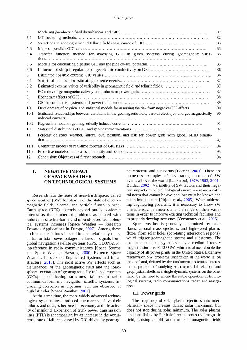
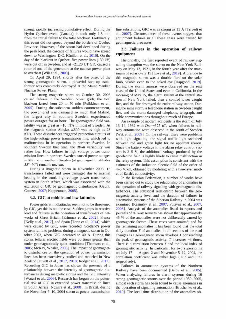
As an example of a substorm during a storm, we
present observations made during a magnetic storm on
March 17, 2013 [Belakhovsky et al., 2018]. It began at
~06 UT, when the solar wind velocity sharply increased
from ~400 to ~650–700 km/s, and IMF became antipar-
allel to the geomagnetic field, which provided reconnec-
tion of fields and a long-term energy input into the
magnetosphere. Amplitude of the |Dst| index, which
characterizes the magnetic storm intensity, was as high
as ~120 nT at the maximum of the storm (~21 UT). The
auroral AE index, which characterizes the auroral elec-
trojet intensity, sharply increased to ~1000 nT. In total,
on March 17 the AE index showed the occurrence of
three auroral activations.
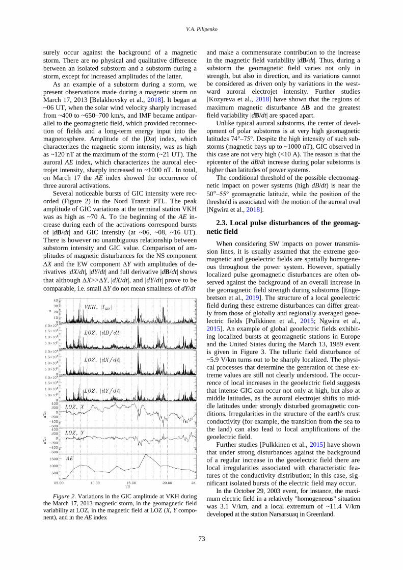
Several noticeable bursts of GIC intensity were rec-
orded (Figure 2) in the Nord Transit PTL. The peak
amplitude of GIC variations at the terminal station VKH
was as high as ~70 A. To the beginning of the AE in-
crease during each of the activations correspond bursts
of |dB/dt| and GIC intensity (at ~06, ~08, ~16 UT).
There is however no unambiguous relationship between
substorm intensity and GIC value. Comparison of am-
plitudes of magnetic disturbances for the NS component
X and the EW component Y with amplitudes of de-
rivatives |dX/dt|, |dY/dt| and full derivative |dB/dt| shows
that although X>>Y, |dX/dt|, and |dY/dt| prove to be
comparable, i.e. small Y do not mean smallness of dY/dt
Figure 2. Variations in the GIC amplitude at VKH during
the March 17, 2013 magnetic storm, in the geomagnetic field
variability at LOZ, in the magnetic field at LOZ (X, Y compo-
nent), and in the AE index
and make a commensurate contribution to the increase
in the magnetic field variability |dB/dt|. Thus, during a
substorm the geomagnetic field varies not only in
strength, but also in direction, and its variations cannot
be considered as driven only by variations in the west-
ward auroral electrojet intensity. Further studies
[Kozyreva et al., 2018] have shown that the regions of
maximum magnetic disturbance B and the greatest
field variability |dB/dt| are spaced apart.
Unlike typical auroral substorms, the center of devel-
opment of polar substorms is at very high geomagnetic
latitudes 74°–75°. Despite the high intensity of such sub-
storms (magnetic bays up to ~1000 nT), GIC observed in
this case are not very high (<10 A). The reason is that the
epicenter of the dB/dt increase during polar substorms is
higher than latitudes of power systems.
The conditional threshold of the possible electromag-
netic impact on power systems (high dB/dt) is near the
50°–55° geomagnetic latitude, while the position of the
threshold is associated with the motion of the auroral oval
[Ngwira et al., 2018].
2.3. Local pulse disturbances of the geomag-
netic field
When considering SW impacts on power transmis-
sion lines, it is usually assumed that the extreme geo-
magnetic and geoelectric fields are spatially homogene-
ous throughout the power system. However, spatially
localized pulse geomagnetic disturbances are often ob-
served against the background of an overall increase in
the geomagnetic field strength during substorms [Enge-
bretson et al., 2019]. The structure of a local geoelectric
field during these extreme disturbances can differ great-
ly from those of globally and regionally averaged geoe-
lectric fields [Pulkkinen et al., 2015; Ngwira et al.,
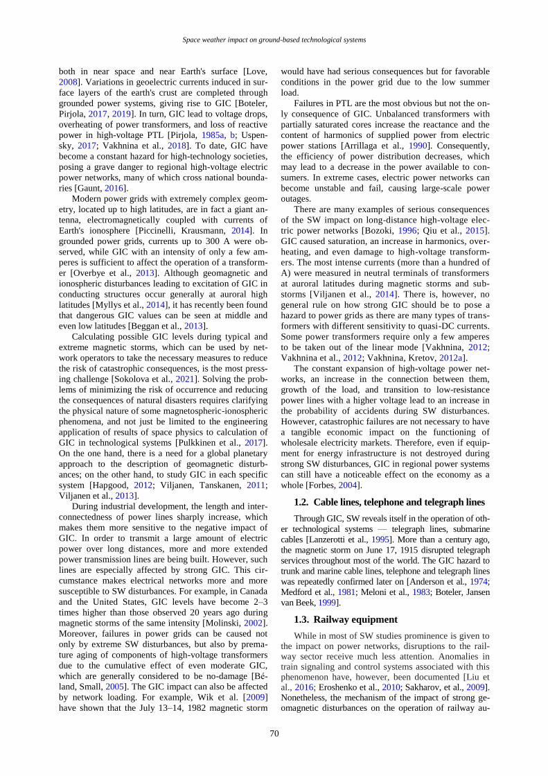
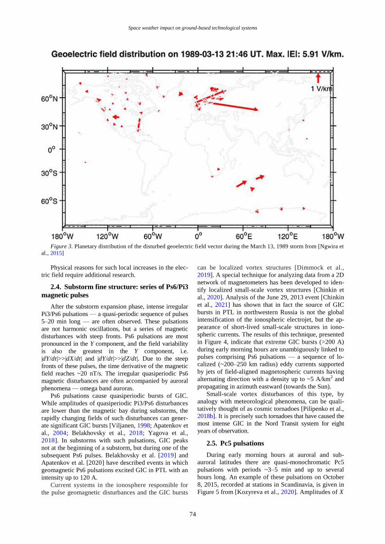
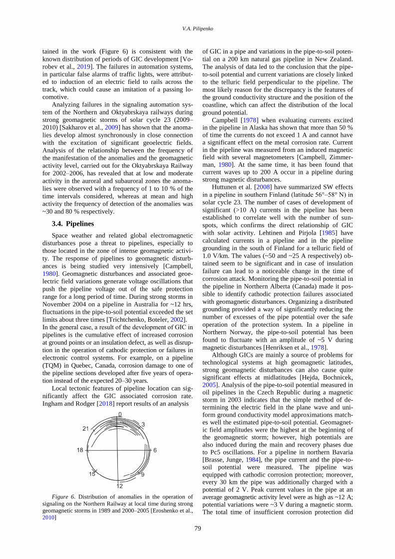
2015]. An example of global geoelectric fields exhibit-
ing localized bursts at geomagnetic stations in Europe
and the United States during the March 13, 1989 event
is given in Figure 3. The telluric field disturbance of
~5.9 V/km turns out to be sharply localized. The physi-
cal processes that determine the generation of these ex-
treme values are still not clearly understood. The occur-
rence of local increases in the geoelectric field suggests
that intense GIC can occur not only at high, but also at
middle latitudes, as the auroral electrojet shifts to mid-
dle latitudes under strongly disturbed geomagnetic con-
ditions. Irregularities in the structure of the earth's crust
conductivity (for example, the transition from the sea to
the land) can also lead to local amplifications of the
geoelectric field.
Further studies [Pulkkinen et al., 2015] have shown
that under strong disturbances against the background
of a regular increase in the geoelectric field there are
local irregularities associated with characteristic fea-
tures of the conductivity distribution; in this case, sig-
nificant isolated bursts of the electric field may occur.
In the October 29, 2003 event, for instance, the maxi-
mum electric field in a relatively "homogeneous" situation
was 3.1 V/km, and a local extremum of ~11.4 V/km
developed at the station Narsarsuaq in Greenland.
Space weather impact on ground-based technological systems
74
Figure 3. Planetary distribution of the disturbed geoelectric field vector during the March 13, 1989 storm from [Ngwira et
al., 2015]
Physical reasons for such local increases in the elec-
tric field require additional research.
2.4. Substorm fine structure: series of Ps6/Pi3
magnetic pulses
After the substorm expansion phase, intense irregular
Pi3/Ps6 pulsations — a quasi-periodic sequence of pulses
5–20 min long — are often observed. These pulsations
are not harmonic oscillations, but a series of magnetic
disturbances with steep fronts. Ps6 pulsations are most
pronounced in the Y component, and the field variability
is also the greatest in the Y component, i.e.
|dY/dt|>>|dX/dt| and |dY/dt|>>|dZ/dt|. Due to the steep
fronts of these pulses, the time derivative of the magnetic
field reaches ~20 nT/s. The irregular quasiperiodic Ps6
magnetic disturbances are often accompanied by auroral
phenomena — omega band auroras.
Ps6 pulsations cause quasiperiodic bursts of GIC.
While amplitudes of quasiperiodic Pi3/Ps6 disturbances
are lower than the magnetic bay during substorms, the
rapidly changing fields of such disturbances can gener-
ate significant GIC bursts [Viljanen, 1998; Apatenkov et
al., 2004; Belakhovsky et al., 2018; Yagova et al.,
2018]. In substorms with such pulsations, GIC peaks
not at the beginning of a substorm, but during one of the
subsequent Ps6 pulses. Belakhovsky et al. [2019] and
Apatenkov et al. [2020] have described events in which
geomagnetic Ps6 pulsations excited GIC in PTL with an
intensity up to 120 A.
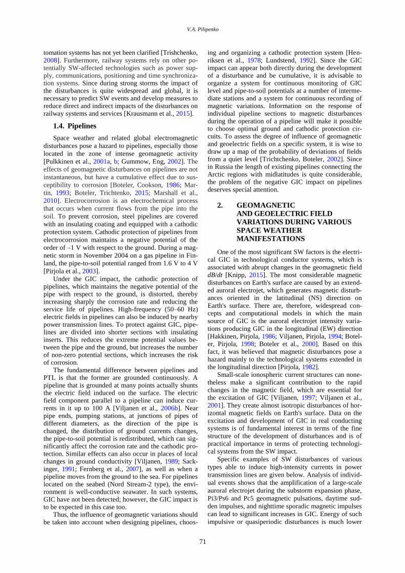
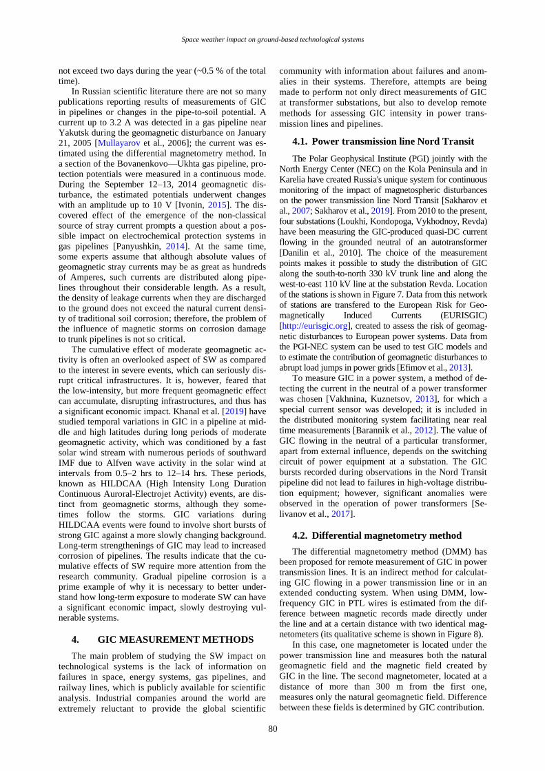
Current systems in the ionosphere responsible for
the pulse geomagnetic disturbances and the GIC bursts
can be localized vortex structures [Dimmock et al.,
2019]. A special technique for analyzing data from a 2D
network of magnetometers has been developed to iden-
tify localized small-scale vortex structures [Chinkin et
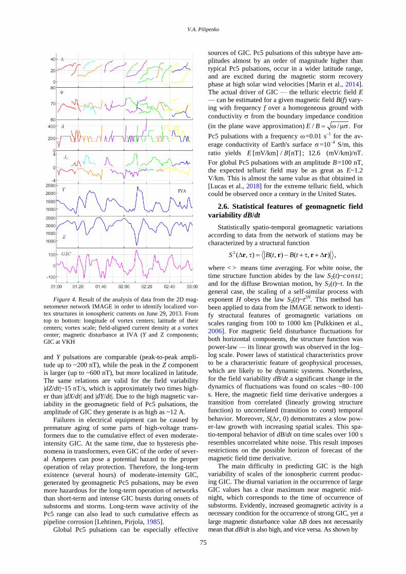
al., 2020]. Analysis of the June 29, 2013 event [Chinkin
et al., 2021] has shown that in fact the source of GIC
bursts in PTL in northwestern Russia is not the global
intensification of the ionospheric electrojet, but the ap-
pearance of short-lived small-scale structures in iono-
spheric currents. The results of this technique, presented
in Figure 4, indicate that extreme GIC bursts (>200 A)
during early morning hours are unambiguously linked to
pulses comprising Ps6 pulsations — a sequence of lo-
calized (~200–250 km radius) eddy currents supported
by jets of field-aligned magnetospheric currents having
alternating direction with a density up to ~5 A/km2 and
propagating in azimuth eastward (towards the Sun).
Small-scale vortex disturbances of this type, by
analogy with meteorological phenomena, can be quali-
tatively thought of as cosmic tornadoes [Pilipenko et al.,
2018b]. It is precisely such tornadoes that have caused the
most intense GIC in the Nord Transit system for eight
years of observation.
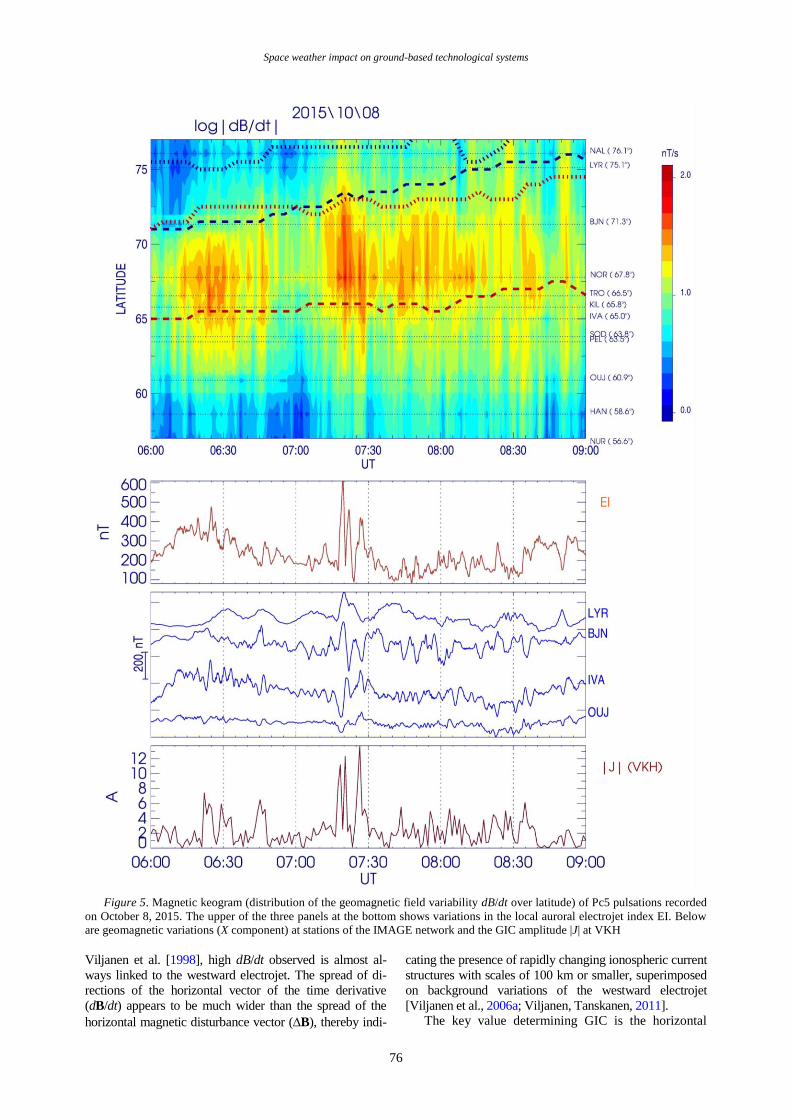
2.5. Pc5 pulsations
During early morning hours at auroral and sub-
auroral latitudes there are quasi-monochromatic Pc5
pulsations with periods ~3–5 min and up to several
hours long. An example of these pulsations on October
8, 2015, recorded at stations in Scandinavia, is given in
Figure 5 from [Kozyreva et al., 2020]. Amplitudes of X
V.A. Pilipenko
75
Figure 4. Result of the analysis of data from the 2D mag-
netometer network IMAGE in order to identify localized vor-
tex structures in ionospheric currents on June 29, 2013. From
top to bottom: longitude of vortex centers; latitude of their
centers; vortex scale; field-aligned current density at a vortex
center; magnetic disturbance at IVA (Y and Z components;
GIC at VKH
and Y pulsations are comparable (peak-to-peak ampli-
tude up to ~200 nT), while the peak in the Z component
is larger (up to ~600 nT), but more localized in latitude.
The same relations are valid for the field variability
|dZ/dt|~15 nT/s, which is approximately two times high-
er than |dX/dt| and |dY/dt|. Due to the high magnetic var-
iability in the geomagnetic field of Pc5 pulsations, the
amplitude of GIC they generate is as high as ~12 A.
Failures in electrical equipment can be caused by
premature aging of some parts of high-voltage trans-
formers due to the cumulative effect of even moderate-
intensity GIC. At the same time, due to hysteresis phe-
nomena in transformers, even GIC of the order of sever-
al Amperes can pose a potential hazard to the proper
operation of relay protection. Therefore, the long-term
existence (several hours) of moderate-intensity GIC,
generated by geomagnetic Pc5 pulsations, may be even
more hazardous for the long-term operation of networks
than short-term and intense GIC bursts during onsets of
substorms and storms. Long-term wave activity of the
Pc5 range can also lead to such cumulative effects as
pipeline corrosion [Lehtinen, Pirjola, 1985].
Global Pc5 pulsations can be especially effective
sources of GIC. Pc5 pulsations of this subtype have am-
plitudes almost by an order of magnitude higher than
typical Pc5 pulsations, occur in a wider latitude range,
and are excited during the magnetic storm recovery
phase at high solar wind velocities [Marin et al., 2014].
The actual driver of GIC — the telluric electric field E
— can be estimated for a given magnetic field B(f) vary-
ing with frequency f over a homogeneous ground with
conductivity from the boundary impedance condition
(in the plane wave approximation) / / .E B For
Pc5 pulsations with a frequency =0.01 s–1
for the av-
erage conductivity of Earth's surface =10–4
S/m, this
ratio yields [mV/km] / [nT 2.] 1 6E В ; (mV/km)/nT.
For global Pc5 pulsations with an amplitude B=100 nT,
the expected telluric field may be as great as E~1.2
V/km. This is almost the same value as that obtained in
[Lucas et al., 2018] for the extreme telluric field, which
could be observed once a century in the United States.
2.6. Statistical features of geomagnetic field
variability dB/dt
Statistically spatio-temporal geomagnetic variations
according to data from the network of stations may be
characterized by a structural function
2 ( , ) ( , ) ( , ) ,S B t B t r r r r
where < > means time averaging. For white noise, the
time structure function abides by the law S2(t)~const ;
and for the diffuse Brownian motion, by S2(t)~t. In the
general case, the scaling of a self-similar process with
exponent H obeys the law S2(t)~t2H
. This method has
been applied to data from the IMAGE network to identi-
fy structural features of geomagnetic variations on
scales ranging from 100 to 1000 km [Pulkkinen et al.,
2006]. For magnetic field disturbance fluctuations for
both horizontal components, the structure function was
power-law — its linear growth was observed in the log–
log scale. Power laws of statistical characteristics prove
to be a characteristic feature of geophysical processes,
which are likely to be dynamic systems. Nonetheless,
for the field variability dB/dt a significant change in the
dynamics of fluctuations was found on scales ~80–100
s. Here, the magnetic field time derivative undergoes a
transition from correlated (linearly growing structure
function) to uncorrelated (transition to const) temporal
behavior. Moreover, S(r, 0) demonstrates a slow pow-
er-law growth with increasing spatial scales. This spa-
tio-temporal behavior of dB/dt on time scales over 100 s
resembles uncorrelated white noise. This result imposes
restrictions on the possible horizon of forecast of the
magnetic field time derivative.
The main difficulty in predicting GIC is the high
variability of scales of the ionospheric current produc-
ing GIC. The diurnal variation in the occurrence of large
GIC values has a clear maximum near magnetic mid-
night, which corresponds to the time of occurrence of
substorms. Evidently, increased geomagnetic activity is a
necessary condition for the occurrence of strong GIC, yet a
large magnetic disturbance value B does not necessarily
mean that dB/dt is also high, and vice versa. As shown by
Space weather impact on ground-based technological systems
76
Figure 5. Magnetic keogram (distribution of the geomagnetic field variability dB/dt over latitude) of Pc5 pulsations recorded
on October 8, 2015. The upper of the three panels at the bottom shows variations in the local auroral electrojet index EI. Below
are geomagnetic variations (X component) at stations of the IMAGE network and the GIC amplitude |J| at VKH
Viljanen et al. [1998], high dB/dt observed is almost al-
ways linked to the westward electrojet. The spread of di-
rections of the horizontal vector of the time derivative
(dB/dt) appears to be much wider than the spread of the
horizontal magnetic disturbance vector (B), thereby indi-
cating the presence of rapidly changing ionospheric current
structures with scales of 100 km or smaller, superimposed
on background variations of the westward electrojet
[Viljanen et al., 2006a; Viljanen, Tanskanen, 2011]. The key value determining GIC is the horizontal
V.A. Pilipenko
77
magnetic field derivative dВ/dt [Oliveira, Ngwira, 2017]. An important question is how closely |dB/dt| is
related to |B|. Knowledge of such relations will help to increase the capability of predicting GIC events because considerable advances have been made in predicting
amplitudes of magnetic disturbances |B| or indices cal-culated from them (e.g., AE). The highest dВ/dt is noted soon after the onset of the substorm expansion phase, although many events later also have higher derivatives. Statistically, the dВ/dt maximum occurs at the fifth mi-nute after the onset of the substorm at geomagnetic lati-tudes of <72° [Viljanen et al., 2006a]. This distribution has, however, a long tail up to tens of minutes. The presence of such long tails in the distribution is charac-teristic of complex multiscale systems. The time of oc-currence of maximum dВ/dt after the onset of a sub-
storm increases with latitude from ~15 min at ~56° to
~45 min at ~75°. In this case, substorms during a storm can have twice the maximum amplitude of |dВ/dt| at all latitudes as compared to isolated substorms.
Statistical laws are somewhat different for isolated sub-storms and substorms during storms. The latitudinal max-imum of |dB/dt| during a storm is ~5° southward than for an isolated substorm, which reflects the well-known equa-torward shift of the auroral oval as magnetic activity in-creases. The median time of occurrence of max(|dB/dt|) increases as a function of latitude for substorms of both
types. Analysis of the relations between max(|B|) and max(|dB/dt|) for substorms of different types shows a high
correlation between |B| and |dВ/dt| — ~0.75 for isolated substorms and ~0.66 for substorms during a storm. The regression curve slope is almost the same for substorms of both types, indicating that the mechanism responsible for
disturbances of В and dВ/dt during substorms does not depend on the presence of a magnetic storm.
The clear majority of the max(|dB/dt|) values are as-sociated with the westward electrojet. The scatter of the dB/dt values means that the rapid changes not always involve the amplification of the electrojet, but often smaller-scale ionospheric structures. The eastward elec-trojet dominates in late afternoon at ~13–21 LT; the westward one, at ~01:30 LT. The diurnal variation in mean dB/dt exhibits an increase during nighttime hours, which is consistent with the electrojet intensity variation. However, the pronounced morning maximum of dB/dt near 05 LT has no analogue in the diurnal variation of the electrojet intensity. The probability of occurrence of large dB/dt val-ues in the vicinity of the eastward electrojet is low.
3. FAILURES IN TECHNOLOGICAL
SYSTEMS CAUSED BY GIC
3.1. Malfunctions in the operation of indus-
trial transformers at auroral latitudes
GIC excited by abrupt changes in the geomagnetic
field are hazardous, first of all, to transformer substa-
tions of high-voltage power transmission lines [Tri-
shchenko, 2008]. Since GICs have a very low frequen-
cy as compared to the industrial frequency 50–60 Hz,
the flow of a quasi-DC current through transformer
windings leads to saturation of magnetic cores of
transformers. The constant current component in a
power transformer also appears when it is switched on;
therefore, power transformer protection relays are usu-
ally adjusted so that not to react to the constant current
component. As a result, conventional relay protection
will not react to GIC saturating the transformer, and it
will simply burn out. In history there are cases of dam-
age to power transformers by GIC during strong mag-
netic storms [Gaunt, Coetzee, 2007], when all over the
world relay protection systems were activated and
blackouts in power transmission lines occurred [Boteler
et al., 1989; Kappenman, 2003, 2005; Pulkkinen et al.,
2003, 2005]. Recovery of power systems after power
outages can take from several hours to several months
(due to the lack of standby power transformers in
many power systems). This is to cause a real collapse
for modern humanity, too dependent on modern tech-
nology and vulnerable to disasters of this kind.
The most intense GIC (up to hundreds of Amperes)
and electric fields in Earth's surface layers (>10 V/m)
are excited at auroral latitudes during magnetic storms
and substorms [Boteler, 2001]. However, accurately
estimating GIC in power transmission lines during a
magnetic storm requires knowledge of the earth's crust
surface layer conductivity and the PTL geometry. Dur-
ing the development of a storm or a substorm against
the background of relatively smooth regularities, ex-
treme bursts of the disturbance amplitude are observed.
From the point of view of ensuring the stable operation
of a power grid, these extreme events can be the most
dangerous. For example, magnetic field variations over
time with dB/dt=1 nT/s induced a current of the order of
several Amperes in Finnish high-voltage networks; and
variations with dB/dt>40 nT/s led to malfunctions in the
operation of Scandinavian energy networks [Viljanen,
Pirjola, 1994]. During magnetospheric disturbances,
multiple cases of excitation of power frequency har-
monics in neutrals of high-voltage autotransformers
were detected, which indicates an overload of trans-
formers, a shift in their operating point, and a threat to
the stable operation of a power grid [Sivokon et al.,
2011]. Here are some examples of catastrophic conse-
quences of strong magnetic storms that occurred in dif-
ferent countries.
The March 13, 1989 magnetic storm caused power
transformer disruption and a total blackout in Hydro-
Québec's electricity transmission system in Canada
[Thomson et al., 2010]. The cost of damage to this sys-
tem alone was about $13 million [Bolduc et al., 1998,
2000; Bolduc, 2002]. This accident left more than six
million people without electricity for eight hours. If
such a storm affected the northeastern United States, the
economic damage could exceed $10 billion [National
Research Council, 2008], not counting serious social
upheavals. This storm is responsible for the overheating
of a power step-up transformer and its outage at the Sa-
lem Nuclear Power Plant (USA). According to [Kap-
penman, 2010], the GIC that caused the transformer to
fail was ~95 A. Since the region covered by the geo-
magnetic storm is large, distortions occur almost simul-
taneously in many transformers. The result may be a
Space weather impact on ground-based technological systems
78
strong, rapidly increasing cumulative effect. During the
Hydro Quebec event (Canada), it took only 1.5 min
from the initial failure to the total blackout. Fortunately,
this event did not spread beyond the borders of Quebec
Province. However, if the storm had developed during
the peak load, the cascade of failures would have spread
down to Washington, D.C. [Guillon et al., 2016]. On the
day of the blackout in Quebec, five power lines (130 kV)
were cut off in Sweden, and at ~21.20 UT GIC caused a
rotor of one of the generators at the nuclear power plant
to overheat [Wik et al., 2008].
On April 29, 1994, shortly after the onset of the
strong geomagnetic storm, a powerful step-up trans-
former was completely destroyed at the Maine Yankee
Nuclear Power Plant.
The strong magnetic storm on October 30, 2003
caused failures in the Swedish power grids; the total
blackout lasted from 20 to 50 min [Pulkkinen et al.,
2005]. During the substorm sudden commencement,
the power grid was damaged so much that Malmö,
the largest city in southern Sweden, experienced
power outages for an hour. The geomagnetic field var-
iability was as great as ~10 nT/s in most of Sweden. At
the magnetic station Abisko, dB/dt was as high as 23
nT/s. These disturbances triggered protection circuits of
the high-voltage power transmission line, which led to
malfunctions in its operation in northern Sweden. In
southern Sweden that time, the dB/dt variability was
rather low. How failures in high voltage power trans-
mission lines in northern Sweden caused power outages
in Malmö in southern Sweden (at geomagnetic latitudes
55°–60°) remains unclear.
During a magnetic storm in November 2003, 15
transformers failed and were damaged due to internal
heating in the trunk high-voltage power transmission
system in South Africa, which was associated with the
excitation of GIC by geomagnetic disturbances [Gaunt,
Coetzee, 2007; Kappenman, 2005].
3.2. GIC at middle and low latitudes
Power grids at midlatitudes seem not to be threatened
by GIC, yet this is not the case. Sudden jumps in reactive
load and failures in the operation of transformers of net-
works of Great Britain [Erinmez et al., 2002], France
[Kelly et al., 2017], and Spain [Torta et al., 2014], which
were caused by GIC, were recorded. Scotland's power
system ran into problems during a magnetic storm in Oc-
tober 2003, when GIC increased to 40 A. During this
storm, telluric electric fields were 50 times greater than
under geomagnetically quiet conditions [Thomson et al.,
2005; McKay, Whaler, 2006]. The impact of geomagnet-
ic disturbances on the operation of power transmission
lines has been extensively studied and modeled in New
Zealand [Divett et al., 2017, 2018; Rodger et al., 2017].
Recording GIC in Japan has shown the presence of a
relationship between the intensity of geomagnetic dis-
turbances during magnetic storms and the GIC intensity
[Watari et al., 2009]. Research has begun on the poten-
tial risk of GIC in extended power transmission lines
in South Africa [Ngwira et al., 2008]. In Brazil, during
the November 7–10, 2004 storm at power transmission
line substations, GIC was as strong as 15 A [Trivedi et
al., 2007]. Circumstances of these events suggest that
equipment failures in all these cases were caused by
geomagnetic processes.
3.3. Failures in the operation of railway
equipment
Historically, the first reported event of railway sig-
naling disruption was the storm on the New York Rail-
way on May 13, 1921, in the fourth year after the max-
imum of solar cycle 15 [Love et al., 2019]. A prelude to
this magnetic storm was a double flare on the solar
limb, visible even to the naked eye [Hapgood, 2019].
During the storm, auroras were observed on the east
coast of the United States and even in California. In the
morning of May 15, the alarm system at the central sta-
tion in New York failed, then a control tower caught
fire, and the fire destroyed the entire railway station. Dur-
ing the same storm, a telephone station in Sweden caught
fire, and the storm damaged telephone, telegraph, and
cable communications throughout much of Europe.
An example of modern accidents is the storm of July
13–14, 1982 with Dst=−325 nT, when failures in rail-
way automation were observed in the south of Sweden
[Wik et al., 2009]. On the railway, there were problems
with light signaling: the signal traffic light switched
between red and green light for no apparent reason.
Since the battery voltage in the alarm relay control sys-
tem is 3–5 V, the additional voltage produced by the
geoelectric field is highly likely to cause malfunction in
the relay system. This assumption is consistent with the
estimates of the induction electric field of the order of
4–5 V/km, obtained by modeling with a two-layer mod-
el of Earth's conductivity.
In the Russian Federation, a number of works have
been carried out to study the relationship of anomalies in
the operation of railway signaling with geomagnetic dis-
turbances. The statistical relationship between the geo-
magnetic activity level and the duration of failures in
automation systems of the Siberian Railway in 2004 was
examined [Kasinsky et al., 2007; Ptitsyna et al., 2007,
2008]. Analysis of the anomalies listed in reports and
journals of railway services has shown that approximately
45 % of the anomalies were not deliberately caused by
geomagnetic factors. These cases were omitted; and for
the remaining anomalies it has been found that the total
daily duration T of anomalies in all sections of the road
changes as a geomagnetic storm develops. Upon reaching
the peak of geomagnetic activity, T increases ~3 times.
There is a correlation between T and the local index of
geomagnetic activity. In particular, for two superstorms
on July 17 — August 2 and November 5–12, 2004, the
correlation coefficient was rather high (0.83 and 0.71
respectively).
Failures in automation systems of the Northern
Railway have been documented [Belov et al., 2005].
When analyzing failures in alarm systems during 16
strong geomagnetic storms over the period 1989–2005,
almost each storm has been found to cause anomalies in
the operation of signaling automation [Eroshenko et al.,
2010]. The local time distribution of the anomalies ob-
V.A. Pilipenko
79
tained in the work (Figure 6) is consistent with the
known distribution of periods of GIC development [Vo-
robev et al., 2019]. The failures in automation systems,
in particular false alarms of traffic lights, were attribut-
ed to induction of an electric field to rails across the
track, which could cause an imitation of a passing lo-
comotive.
Analyzing failures in the signaling automation sys-
tem of the Northern and Oktyabrskaya railways during
strong geomagnetic storms of solar cycle 23 (2009–
2010) [Sakharov et al., 2009] has shown that the anoma-
lies develop almost synchronously in close connection
with the excitation of significant geoelectric fields.
Analysis of the relationship between the frequency of
the manifestation of the anomalies and the geomagnetic
activity level, carried out for the Oktyabrskaya Railway
for 2002–2006, has revealed that at low and moderate
activity in the auroral and subauroral zones the anoma-
lies were observed with a frequency of 1 to 10 % of the
time intervals considered, whereas at mean and high
activity the frequency of detection of the anomalies was
~30 and 80 % respectively.
3.4. Pipelines
Space weather and related global electromagnetic
disturbances pose a threat to pipelines, especially to
those located in the zone of intense geomagnetic activi-
ty. The response of pipelines to geomagnetic disturb-
ances is being studied very intensively [Campbell,
1980]. Geomagnetic disturbances and associated geoe-
lectric field variations generate voltage oscillations that
push the pipeline voltage out of the safe protection
range for a long period of time. During strong storms in
November 2004 on a pipeline in Australia for ~12 hrs,
fluctuations in the pipe-to-soil potential exceeded the set
limits about three times [Trichtchenko, Boteler, 2002].
In the general case, a result of the development of GIС in
pipelines is the cumulative effect of increased corrosion
at ground points or an insulation defect, as well as disrup-
tion in the operation of cathodic protection or failures in
electronic control systems. For example, on a pipeline
(TQM) in Quebec, Canada, corrosion damage to one of
the pipeline sections developed after five years of opera-
tion instead of the expected 20–30 years.
Local tectonic features of pipeline location can sig-
nificantly affect the GIC associated corrosion rate.
Ingham and Rodger [2018] report results of an analysis
Figure 6. Distribution of anomalies in the operation of
signaling on the Northern Railway at local time during strong
geomagnetic storms in 1989 and 2000–2005 [Eroshenko et al.,
2010]
of GIC in a pipe and variations in the pipe-to-soil poten-
tial on a 200 km natural gas pipeline in New Zealand.
The analysis of data led to the conclusion that the pipe-
to-soil potential and current variations are closely linked
to the telluric field perpendicular to the pipeline. The
most likely reason for the discrepancy is the features of
the ground conductivity structure and the position of the
coastline, which can affect the distribution of the local
ground potential.
Campbell [1978] when evaluating currents excited in the pipeline in Alaska has shown that more than 50 % of time the currents do not exceed 1 A and cannot have a significant effect on the metal corrosion rate. Current in the pipeline was measured from an induced magnetic field with several magnetometers [Campbell, Zimmer-man, 1980]. At the same time, it has been found that current waves up to 200 A occur in a pipeline during strong magnetic disturbances.
Huttunen et al. [2008] have summarized SW effects
in a pipeline in southern Finland (latitude 56°–58° N) in
solar cycle 23. The number of cases of development of
significant (>10 A) currents in the pipeline has been
established to correlate well with the number of sun-
spots, which confirms the direct relationship of GIC
with solar activity. Lehtinen and Pirjola [1985] have
calculated currents in a pipeline and in the pipeline
grounding in the south of Finland for a telluric field of
1.0 V/km. The values (~50 and ~25 A respectively) ob-
tained seem to be significant and in case of insulation
failure can lead to a noticeable change in the time of
corrosion attack. Monitoring the pipe-to-soil potential in
the pipeline in Northern Alberta (Canada) made it pos-
sible to identify cathodic protection failures associated
with geomagnetic disturbances. Organizing a distributed
grounding provided a way of significantly reducing the
number of excesses of the pipe potential over the safe
operation of the protection system. In a pipeline in
Northern Norway, the pipe-to-soil potential has been
found to fluctuate with an amplitude of ~5 V during
magnetic disturbances [Henriksen et al., 1978]. Although GICs are mainly a source of problems for
technological systems at high geomagnetic latitudes, strong geomagnetic disturbances can also cause quite significant effects at midlatitudes [Hejda, Bochnicek, 2005]. Analysis of the pipe-to-soil potential measured in oil pipelines in the Czech Republic during a magnetic storm in 2003 indicates that the simple method of de-termining the electric field in the plane wave and uni-form ground conductivity model approximations match-es well the estimated pipe-to-soil potential. Geomagnet-ic field amplitudes were the highest at the beginning of the geomagnetic storm; however, high potentials are also induced during the main and recovery phases due to Pc5 oscillations. For a pipeline in northern Bavaria [Brasse, Junge, 1984], the pipe current and the pipe-to-soil potential were measured. The pipeline was equipped with cathodic corrosion protection; moreover, every 30 km the pipe was additionally charged with a potential of 2 V. Peak current values in the pipe at an average geomagnetic activity level were as high as ~12 A; potential variations were ~3 V during a magnetic storm. The total time of insufficient corrosion protection did
Space weather impact on ground-based technological systems
80
not exceed two days during the year (~0.5 % of the total time).
In Russian scientific literature there are not so many publications reporting results of measurements of GIC in pipelines or changes in the pipe-to-soil potential. A current up to 3.2 A was detected in a gas pipeline near Yakutsk during the geomagnetic disturbance on January 21, 2005 [Mullayarov et al., 2006]; the current was es-timated using the differential magnetometry method. In a section of the Bovanenkovo—Ukhta gas pipeline, pro-tection potentials were measured in a continuous mode. During the September 12–13, 2014 geomagnetic dis-turbance, the estimated potentials underwent changes with an amplitude up to 10 V [Ivonin, 2015]. The dis-covered effect of the emergence of the non-classical source of stray current prompts a question about a pos-sible impact on electrochemical protection systems in gas pipelines [Panyushkin, 2014]. At the same time, some experts assume that although absolute values of geomagnetic stray currents may be as great as hundreds of Amperes, such currents are distributed along pipe-lines throughout their considerable length. As a result, the density of leakage currents when they are discharged to the ground does not exceed the natural current densi-ty of traditional soil corrosion; therefore, the problem of the influence of magnetic storms on corrosion damage to trunk pipelines is not so critical.
The cumulative effect of moderate geomagnetic ac-tivity is often an overlooked aspect of SW as compared to the interest in severe events, which can seriously dis-rupt critical infrastructures. It is, however, feared that the low-intensity, but more frequent geomagnetic effect can accumulate, disrupting infrastructures, and thus has a significant economic impact. Khanal et al. [2019] have studied temporal variations in GIC in a pipeline at mid-dle and high latitudes during long periods of moderate geomagnetic activity, which was conditioned by a fast solar wind stream with numerous periods of southward IMF due to Alfven wave activity in the solar wind at intervals from 0.5–2 hrs to 12–14 hrs. These periods, known as HILDCAA (High Intensity Long Duration Continuous Auroral-Electrojet Activity) events, are dis-tinct from geomagnetic storms, although they some-times follow the storms. GIC variations during HILDCAA events were found to involve short bursts of strong GIC against a more slowly changing background. Long-term strengthenings of GIC may lead to increased corrosion of pipelines. The results indicate that the cu-mulative effects of SW require more attention from the research community. Gradual pipeline corrosion is a prime example of why it is necessary to better under-stand how long-term exposure to moderate SW can have a significant economic impact, slowly destroying vul-nerable systems.
4. GIC MEASUREMENT METHODS
The main problem of studying the SW impact on
technological systems is the lack of information on
failures in space, energy systems, gas pipelines, and
railway lines, which is publicly available for scientific
analysis. Industrial companies around the world are
extremely reluctant to provide the global scientific
community with information about failures and anom-
alies in their systems. Therefore, attempts are being
made to perform not only direct measurements of GIC
at transformer substations, but also to develop remote
methods for assessing GIC intensity in power trans-
mission lines and pipelines.
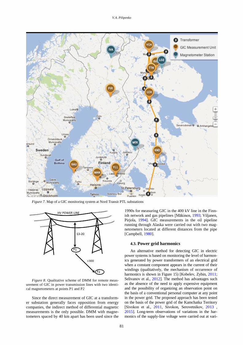
4.1. Power transmission line Nord Transit
The Polar Geophysical Institute (PGI) jointly with the
North Energy Center (NEC) on the Kola Peninsula and in
Karelia have created Russia's unique system for continuous
monitoring of the impact of magnetospheric disturbances
on the power transmission line Nord Transit [Sakharov et
al., 2007; Sakharov et al., 2019]. From 2010 to the present,
four substations (Loukhi, Kondopoga, Vykhodnoy, Revda)
have been measuring the GIC-produced quasi-DC current
flowing in the grounded neutral of an autotransformer
[Danilin et al., 2010]. The choice of the measurement
points makes it possible to study the distribution of GIC
along the south-to-north 330 kV trunk line and along the
west-to-east 110 kV line at the substation Revda. Location
of the stations is shown in Figure 7. Data from this network
of stations are transfered to the European Risk for Geo-
magnetically Induced Currents (EURISGIC)
[http://eurisgic.org], created to assess the risk of geomag-
netic disturbances to European power systems. Data from
the PGI-NEC system can be used to test GIC models and
to estimate the contribution of geomagnetic disturbances to
abrupt load jumps in power grids [Efimov et al., 2013].
To measure GIC in a power system, a method of de-
tecting the current in the neutral of a power transformer
was chosen [Vakhnina, Kuznetsov, 2013], for which a
special current sensor was developed; it is included in
the distributed monitoring system facilitating near real
time measurements [Barannik et al., 2012]. The value of
GIC flowing in the neutral of a particular transformer,
apart from external influence, depends on the switching
circuit of power equipment at a substation. The GIC
bursts recorded during observations in the Nord Transit
pipeline did not lead to failures in high-voltage distribu-
tion equipment; however, significant anomalies were
observed in the operation of power transformers [Se-
livanov et al., 2017].
4.2. Differential magnetometry method
The differential magnetometry method (DMM) has been proposed for remote measurement of GIC in power transmission lines. It is an indirect method for calculat-ing GIC flowing in a power transmission line or in an extended conducting system. When using DMM, low-frequency GIC in PTL wires is estimated from the dif-ference between magnetic records made directly under the line and at a certain distance with two identical mag-netometers (its qualitative scheme is shown in Figure 8).
In this case, one magnetometer is located under the
power transmission line and measures both the natural
geomagnetic field and the magnetic field created by
GIC in the line. The second magnetometer, located at a
distance of more than 300 m from the first one,
measures only the natural geomagnetic field. Difference
between these fields is determined by GIC contribution.
V.A. Pilipenko
81
Figure 7. Map of a GIC monitoring system at Nord Transit PTL substations
Figure 8. Qualitative scheme of DMM for remote meas-
urement of GIC in power transmission lines with two identi-
cal magnetometers at points P1 and P2
Since the direct measurement of GIC at a transform-er substation generally faces opposition from energy companies, the indirect method of differential magnetic measurements is the only possible. DMM with magne-tometers spaced by 40 km apart has been used since the
1990s for measuring GIC in the 400 kV line in the Finn-ish network and gas pipelines [Mäkinen, 1993; Viljanen, Pirjola, 1994]. GIC measurements in the oil pipeline running through Alaska were carried out with two mag-netometers located at different distances from the pipe [Campbell, 1980].
4.3. Power grid harmonics
An alternative method for detecting GIC in electric
power systems is based on monitoring the level of harmon-
ics generated by power transformers of an electrical grid
when a constant component appears in the current of their
windings (qualitatively, the mechanism of occurrence of
harmonics is shown in Figure 15) [Kobelev, Zybin, 2011;
Selivanov et al., 2012]. The method has advantages such
as the absence of the need to apply expensive equipment
and the possibility of organizing an observation point on
the basis of a conventional personal computer at any point
in the power grid. The proposed approach has been tested
on the basis of the power grid of the Kamchatka Territory
[Sivokon et al., 2011, Sivokon, Serovetnikov, 2013 ,
2015]. Long-term observations of variations in the har-
monics of the supply-line voltage were carried out at vari-
Space weather impact on ground-based technological systems
82
ous observation points, characterized by different supply
line topology and system load conditions. Results have
been obtained which confirm the relationship of variations
in the level of power grid harmonics with geomagnetic
disturbances.
4.4. GIC in power grids and VLF radio
emission
VLF radio receivers can be a means of remote detec-
tion of GIC in power grids. When transformers are
loaded with GIC, they generate high harmonics of 50–
60 Hz alternating current flowing through these grids.
Part of the power of these harmonics is emitted as radio
waves at frequencies up to several kHz and is even de-
tected by satellites. Existence of these VLF emissions in
a power grid was first discovered more than forty years
ago. However, in those years the interest in SW and
GIC was very limited, in contrast to the present day
when these issues are of global concern. Clilverd et al.
[2018] have reminded in time that industrial network
frequency harmonic VLF emissions have significant
potential as a diagnostic tool for monitoring GIС in
power grids without intervention in network equipment.
This can provide significant practical advantages in
terms of safety and cost.
5. MODELING GEOELECTRIC
FIELD DISTURBANCES
AND GIC
Modern power systems are a huge network with an ex-
tremely complex topology that covers vast areas of Earth's
surface whose local geoelectric properties (for example,
conductivity) can differ by several orders of magnitude. In
media with low conductivity, the occurrence rate of nega-
tive effects of strong magnetic disturbances increases
sharply since induced currents mainly flow through con-
ductive elements of industrial networks. Geoelectric fields
induced in Earth's surface during magnetic storms can af-
fect the operation of electrical networks. The danger re-
mains that the occurrence of an extreme magnetic storm in
the future could lead to a large-scale loss of energy capaci-
ty, which will significantly affect the economies of coun-
tries at risk.
Attempts to develop devices blocking GIC in a large
electrical network have not yet yielded results. There-
fore, the main hopes are pinned on the on-line control
and prevention of relatively rare problems associated
with strong magnetic storms. The potential difference in
the surface layers of the earth's crust causes overloads in
grounded electric power grids. It is however difficult to
get direct information on geoelectric fields. While geo-
magnetic variations are tracked by the worldwide net-
work of magnetometers (>300), regular observations of
telluric electric fields are still extremely rare. Long-term
measurements of the geoelectric field at observatories are
much rarer. Since 1983, such observations of the geoelec-
tric field have been made only at observatories by the Ja-
pan Meteorological Agency, Geo Forschungs Zentrum
(Germany), the British Geological Survey (UK), and the
Institute of Earth Physics of Paris (France).
5.1. Magnetotelluric sounding methods
Correct calculation of telluric electric fields and cur-
rents requires a sufficiently dense network of magne-
tometers and information about the geoelectric section
of the earth's crust. There is no optimal global model of
the geoelectric conductivity; therefore, various approx-
imate schemes have to be used for the calculations [Bo-
teler et al., 1998]. Comparison between the methods has
shown that the impedance relation in the plane wave
and plane geometry approximations may be employed
to calculate telluric fields with high accuracy [Pirjola,
2002; Viljanen et al., 2015]. This approximation is valid
under the assumption that the horizontal scale of the
disturbance is much larger than the skin length [Wait,
1982]. The situation is greatly simplified by the fact that
integral estimates of the potential difference between
nodes of an extended system (at least several hundred
kilometers) are important for GIC calculations, and
hence the required estimates can also be made with suf-
ficient accuracy in a network of relatively widely spaced
magnetometers with a crude conductivity model [Beg-
gan, 2015].
The main cause of GIC is the geoelectric field that in
the plane wave approximation is related to geomagnetic
variations through the surface impedance of Earth's surface
[Liu et al., 2009; Boteler, Pirjola, 2019]. Impedance is
determined by the depth distribution of electrical conduc-
tion in the earth's crust. The magnetic field variability
dB/dt is more sensitive to local anomalies in the conductiv-
ity of the underlying surface than B [Thomson et al.,
2009]. The electrical conductivity ranges from 10–4
within the earth's interior to 3 S/m2 in the ocean. Power
grids are most sensitive to interference from natural geoe-
lectric fields with periods from 10 to 1000 s. Variations in
geomagnetic and geoelectric fields with such periods pene-
trate into Earth's surface layers to a depth of the order of
the skin length ranging from 2 to 3000 km.
Direct measurement of the geoelectric field E is conceptually simple: it is proportional to the potential difference between a pair of buried electrodes. For magnetotelluric (MT) studies, geoelectric measurements are usually carried out with a magnetic variometer. Qualitatively, the interaction of an electromagnetic dis-turbance with the earth's crust can be represented as
leakage of an incident wave with a frequency to a
depth of order of skin length . If the horizontal scale of a disturbance is much larger than the skin length (strong skin effect condition), the impedance relation
E()=Z()H() between spectral amplitudes of vectors of horizontal electric E={Ex, Ey} and magnetic B={X,
Y} components is valid for Earth's surface. Here, Z() is the surface impedance determined by Earth's internal
resistivity distribution (z). For a homogeneous earth's
crust, the impedance 0Z depends on the period
of geomagnetic disturbance T as 1/2( ) .Z T T The
telluric field E can be synthesized from measured geo-magnetic variations, using the impedance relation in the frequency domain between the horizontal components
of electric E() and magnetic B() fields through the
V.A. Pilipenko
83
complex impedance tensor Z() as follows
1
0
( ) ( ).
( ) ( )
x xx xy
y yx yy
E Z Z X
E Z Z Y
(1)
Information on the impedance of Earth's surface re-
quires preliminary MT sounding, which has been done
only for certain areas of Earth's surface. Calculations of
the telluric field are significantly complicated for a 3D
inhomogeneous medium or for high-resistivity rocks,
where the strong skin effect condition is not met [Kel-
bert et al., 2017].
To date, the most advanced model of planetary litho-
sphere conductivity distribution is the 3D model
[Kuvshinov, Olsen, 2006]. It has been exploited to cal-
culate the planetary distribution of telluric fields from
large-scale magnetospheric sources [Kuvshinov, 2008].
Peak values of the telluric fields are as high as ~50
mV/km for a storm with Dst~300 nT at midlatitudes
(<55°). Nonetheless, this model cannot be applied to
high latitudes, where more intense disturbances are gen-
erated by more localized and dynamic substorm pro-
cesses. For example, >80 % of the spectral power of
geomagnetic variations at auroral latitudes is concen-
trated on time scales of <8 min [Wintoff, 2005].
5.2. Variations in geomagnetic and telluric
fields as a source of GIC
The GIC intensity J was generally assumed to be
proportional to the time derivative of the geomagnetic
field, J~dB/dt. But this relationship is valid for a closed
circuit only in free space. In real situations, the circuit
through which GIC flows is formed by power transmis-
sion lines, ground contacts, terminal transformers, and
the ground. Electrical parameters of these elements, as
well as their frequency dependence, are known very
approximately. The actual relationship between the
spectral composition of magnetic variations B, telluric
electric field E, and current J should be studied for each
power system separately [Bonner, Schultz, 2017].
An example of such a study for the Nord Transit system
is given in [Kozyreva et al., 2019]. The results from the
following groups of stations are presented here: closely
located LOZ—B50—RVD sites, and magnetic and GIC
stations at the same geomagnetic latitudes IVA—VKH
(Figure 9). Telluric electric fields have been calculated
using available impedance data in the range of periods
8–5000 s from the BEAR experiment results [Korja et
al., 2002]. The spatial distribution of the electrical con-
ductivity in the Eastern Baltic shield is very inhomoge-
neous. Comparison between impedances of several
characteristic sections is shown in Figure 10. For the
period T=90.5 s, the largest value of the impedance
modulus |Z| falls on the region of the PEL/B31 stations
(~10 mV/kmnT), whereas in the vicinity of the
OUJ/B33 stations the impedance is ~4 times lower (~2.4
mV/kmnT).
Thus, for the same magnetic disturbance, the con-
trast of a telluric electric field between different points
may be as high as 3–4 times. The significant values of both
diagonal and off-diagonal elements of Z tensor indicate
Figure 9. Magnetic stations IMAGE (black dots), selected
points of MT sounding in the BEAR project (triangles), and
GIC detection stations in the Nord Transit power transmission
line
that geoelectric properties of the earth's crust are highly
anisotropic. Time series of the synthesized telluric fields
have been calculated using the Fourier transform of
magnetic variations with the removed trend from im-
pedance relation (1), and the subsequent inverse Fourier
transform from the spectrum convolution B(f) with the
impedance Z(f).
The magnetic storm on November 12–14, 2012
(|SYM-H|>100 nT) was triggered by fast solar wind
streams. In November 14 at 00–04 UT, a series of en-
hancements of the local electrojet took place (EI~1500
nT). During this period, intense GIC variations were
recorded in all PTL elements, and up to ~60 A at the
terminal station VKH. The J bursts occurred synchro-
nously with an increase in dX/dt to ~10 nT/s and in the
telluric field to several V/km.
Even the visual comparison in Figure 11 shows that
the dX(t)/dt fluctuations are more high-frequency than
those of E(t) and J(t). Spectral analysis of simultaneous
geomagnetic, telluric, and GIC variations (Figure 12)
confirms this fact. Spectral components at frequencies of
~4 and ~6 mHz were identified in the spectrum of J(f)
and X(f)(X=dX/dt). These components are due to the
contribution of fast Pi3 fluctuations superimposed on an
enhancement of the auroral electrojet. As such, the X(f)
spectrum deviates considerably from the J(f) spectrum at
frequencies of >5 mHz and appears to be much closer to
the Ex(f) spectrum. Thus, the geoelectric properties serve
as a filter that diminishes the influence of high frequen-
cies of dB/dt.
5.3. Maps of possible GIC values
Information about geoelectrical resistance is a big
problem for geoelectric mapping because conductivity
of the earth's crust fluctuates by at least four orders of
Space weather impact on ground-based technological systems
84
Figure 10. Amplitudes of impedance tensor elements Zi, j (the X-axis is directed to the north; Y-axis, to the east) as a function
of T at some BEAR stations
Figure 11. GIC intensity J[A] at VKH, magnetic varia-
tions in X[nT], time derivative dX/dt [nT/s] at IVA, and tellu-
ric fields Ex [V/km] and Ey [V/km] at IVA/B5
Figure 12. Normalized spectra for the 01–03 UT interval
of the November 14, 2012 event: J(f) at VKH, X(f), X(f),
and Ex(f) at IVA
magnitude. In 2006 under the EarthScope Project
[https://www.earthscope.org], an MT survey of the
United States on a network of stations spaced by 70 km
apart was launched [Schultz et al., 2009]. The project
ended in 2018 when the MT sounding of approximately
2/3 of the United States had been completed. For each
location, mobile facilities were deployed which includ-
ed a fluxgate magnetometer and a pair of electric di-
poles to measure three magnetic field components and
two horizontal electric field components [Love et al.,
2017]. Then, simultaneous measurements of geomag-
netic and geoelectric fields were used to calculate the
magnetotelluric impedance tensor as a function of fre-
quency Z(ω). The impedance tensors obtained from sur-
vey areas cover the range of periods from 10 to 20000 s
with an estimated error of less than 5 %.
The empirical impedance tensors obtained from
EarthScope MT data were used to explore the possibility of
mapping geoelectric fields induced by magnetic disturb-
ances and to identify Earth's conductivity effects [Bed-
rosian, Love, 2015]. The US Geological Survey has creat-
ed a map of synthetic geoelectric fields that could be excit-
ed by a given spatially homogeneous geomagnetic disturb-
ance. Such a map allows one to quickly assess the possible
risks from GIC during different expected disturbances. For
geomagnetic oscillations with T=100 s, induced geoelectric
field vectors exhibit significant differences in amplitude
(up to 100 times), direction (up to 130°), and phase (more
than a quarter of the wavelength) in different regions (Fig-
ure 13). Horizontal geoelectric field vectors E induced by a
sinusoidal geomagnetic field Bx(t) with 1 nT amplitude
range from 1.2 to 33.5 mV/km.
Love et al. [2016, 2018] have estimated possible ex-treme variability in the geomagnetic field and geoelec-tric currents for the mid-latitude part of the United States. From the analysis of the MT survey data and the
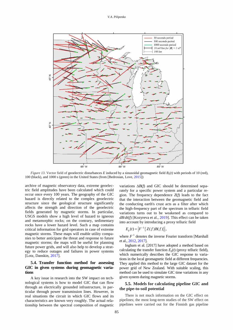
V.A. Pilipenko
85
Figure 13. Vector field of geoelectric disturbances E induced by a sinusoidal geomagnetic field Bx(t) with periods of 10 (red),
100 (black), and 1000 s (green) in the United States (from [Bedrosian, Love, 2015])
archive of magnetic observatory data, extreme geoelec-tric field amplitudes have been calculated which could occur once every 100 years. The geography of the GIC hazard is directly related to the complex geoelectric structure since the geological structure significantly affects the strength and direction of the geoelectric fields generated by magnetic storms. In particular, USGS models show a high level of hazard to igneous and metamorphic rocks; on the contrary, sedimentary rocks have a lower hazard level. Such a map contains critical information for grid operators in case of extreme magnetic storms. These maps will enable utility compa-nies to better anticipate the threat and response to future magnetic storms; the maps will be useful for planning future power grids, and will also help to develop a strat-egy to reduce outages and failures in power systems [Lotz, Danskin, 2017].
5.4. Transfer function method for assessing
GIC in given systems during geomagnetic varia-tions
A key issue in research into the SW impact on tech-
nological systems is how to model GIC that can flow
through an electrically grounded infrastructure, in par-
ticular through power transmission lines. However, in
real situations the circuit in which GIC flows and its
characteristics are known very roughly. The actual rela-
tionship between the spectral composition of magnetic
variations B(f) and GIC should be determined sepa-
rately for a specific power system and a particular re-
gion. The frequency dependence Z(f) leads to the fact
that the interaction between the geomagnetic field and
the conducting earth's crust acts as a filter after which
the high-frequency part of the spectrum in telluric field
variations turns out to be weakened as compared to
dB/dt(f) [Kozyreva et al., 2019]. This effect can be taken
into account by introducing a proxy telluric field
1
p ( ) ( ) ( ) ,E t F Z f B f
where F–1
denotes the inverse Fourier transform [Marshall
et al., 2012, 2017].
Ingham et al. [2017] have adopted a method based on
calculating the transfer function Ep(t) (proxy telluric field),
which numerically describes the GIC response to varia-
tions in the local geomagnetic field at different frequencies.
They applied this method to the large GIC dataset for the
power grid of New Zealand. With suitable scaling, this
method can be used to simulate GIC time variations in any
given system during magnetic storms.
5.5. Models for calculating pipeline GIC and
the pipe-to-soil potential
There is not much information on the GIC effect on
pipelines; the most long-term studies of the SW effect on
pipelines were carried out for the Finnish gas pipeline
Space weather impact on ground-based technological systems
86
from 1998 to 1999 [Pulkkinen et al., 2001a, b]. They
were aimed at developing a model for assessing GIC in
the pipeline and the pipe-to-soil potential and for obtain-
ing statistical predictions of GIC and potentials in differ-
ent parts of the pipeline network [Lundstend, 2006]. The
study has shown the greatest changes in the pipe-to-soil
potential occur at ends of the pipelines, whereas the
strongest GIC are in middle parts of the pipelines.
Currents in conducting systems have been calculated using the DSTL method (Distributed-Source Transmis-sion Line) [Boteler, 1997], the method of complex imag-es [Pirjola, Viljanen, 1998], the method of matrix equa-tions [Lehtinen, Pirjola, 1985], the method of source elementary current systems [Viljanen et al., 1999, 2004], and the transmission line method in which the conductivi-ty matrix in the pipeline model is constructed taking into account grounding parameters of individual pipeline sections and branches [Boteler, 2013]. The calculations have shown that the telluric voltage depends not only on the telluric field direction and magnitude but also on the length and grounding resistance of the pipe. These cal-culations, applied to modern pipelines with good coat-ing, suggest that the effect of telluric currents may not be as harmless as originally assumed [Gummow, Eng, 2002].
5.6. Influence of sharp irregularities of geoe-
lectric conductivity
Assessing the SW effect on power grids in coastal
regions requires taking into account features of the con-
ductivity structure. Risk assessments should involve
assessments of whether the geoelectric fields produced
by geomagnetic disturbances can increase on the coast,
affecting power transmission lines in coastal areas.
Tozzi et al. [2019] have assessed the risk from SW for
the Italian power grid. It consists of 380–400 and 220–
275 kV transmission lines, as well as a high-voltage DC
transmission line running under the sea surface to the
island of Sardinia. The authors show that strong GIC
can flow in power systems even at low geomagnetic
latitudes during magnetic storms and substorms. Taking
into account the proximity of the coast increases the
estimate of expected telluric fields and GIC.
Telluric fields for the real 3D inhomogeneous structure of the conductivity of the earth's crust and upper mantle during magnetic storms have been mod-eled in [Marshalko et al., 2020]. Using a combined approach involving 3D modeling of electromagnetic field and magnetohydrodynamic (MHD) modeling of NES, the dynamics of telluric fields during the March 17, 2015 magnetic storm was successfully simulated. Various conductivity models were adopted including the realistic 3D model derived from EarthScope pro-ject data. Conductivity contrasts were shown to have a great effect not only on the local telluric field, but also on the global distribution of the electric field potential and hence on GIC. Comparison of modeling for the realistic spatially inhomogeneous and plane-wave ap-proximation, which is the most common approach to modeling GIC, has revealed significant differences between results even at midlatitudes. The difference is especially large at boundaries of conductivity contrasts.
Joint MT research and soil-to-pipe potential distribu-
tion study are a useful tool for identifying potential GIC
hazards to pipelines. When modeling soil-to-pipe poten-
tial variations based on the distributed-source transmis-
sion line theory, a good fit with the potential observed
can be obtained if impedance jumps are taken into ac-
count. Thus, the large difference between soil-to-pipe
potentials is due to the presence of resistive intrusive
bodies in the upper crust. In particular, an abnormally
high potential between pipe and soil is observed along
the gas pipeline in eastern Ontario (Canada), where the
geological contact runs between highly resistive rocks
and more conductive sediments, which supports the
hypothesis that considerable potential variations are
linked to changes in the ground conductivity around the
pipeline.
6. ESTIMATED POSSIBLE
EXTREME GIC VALUES
The problem of estimating the probability of ex-
treme GIC is a part of the more general problem of de-
termining the probability of extreme geophysical events
(earthquakes and magnetic storms) [Coles, Lam, 1998;
Love, 2012]. The most intense magnetic storm, the Car-
rington event, occurred on September 1–2, 1859. During
that storm, auroras were seen even in Hawaii, a maxi-
mum geomagnetic disturbance H~1600 nT was rec-
orded at the equatorial station Bombay, and the Dst in-
dex was estimated as –850 nT. After the beginning of
the space age in 1957, the strongest magnetic storm with
|Dst|~590 nT occurred on March 13, 1989. Other histor-
ically powerful storms were observed on July 4, 1941
(H>700 nT) and March 24, 1940 (H>660 nT) [Wei
et al., 2013].
Attempts have been made to assess the probability
of recurrence of such events [Cid et al., 2015]. Riley
[2012] has estimated the probability of recurrence of a
Carrington-type storm over the next decade at 12 %.
Tsubouchi and Omura [2007] believe that storms simi-
lar to that occurring in 1989 can happen once every 60
years. Statistical analysis of the archive of magnetic storm
records (more than hundred events with H>100 nT)
at Kakioka Observatory since 1924 for 89 years has
estimated the probability of a Carrington level storm in
the next decade at ~13 %. If a storm like the storm of
March 13, 1989 or January 09, 1859 occurred today, it
would create serious problems in the operation of tech-
nological systems around the world. According to some
possible scenarios, the occurrence of a rare and abnor-
mally powerful storm will cause an avalanche of outag-
es and failures in power grids, possibly destructive to
economies of developed countries [National Research
Council, 2008].
However, if we assume that extreme magnetic dis-
turbances simply exceed the maximum values observed
during instrumental observations a given number of
times (10, 3), adjusting to such unreasonably large
values would require unnecessary expenses. The value
that occurs once every 100 years is supposed to be taken
as extreme GIC [Pulkkinen et al., 2008, 2012]. An ex-
V.A. Pilipenko
87
treme event is estimated by analyzing the statistical dis-
tribution of the occurrence rate of disturbances of given
amplitude for a region under study. It is approximation
of the dependence of the occurrence rate per event once
every 100 years that gives the extreme value for a given
region [Bernabeu, 2013]. By analyzing the archive of
geomagnetic data, we can estimate the occurrence rate
of extreme geomagnetic disturbances at different lati-
tudes. By combining the data, it is possible to compile a
regional map of geomagnetic risks, similar to the seis-
mic hazard map — the maximum possible number of
geoelectric disturbances once a century. This approach
is used to estimate extreme telluric fields and GIC for
different regions [Langlois et al., 1996].
6.1. Statistical methods for estimating ex-
treme events
The form of the probability function F(x) of disturb-
ance amplitude x is determined by physical mechanisms
of the process under study. Thus, under random inde-
pendent effects a normal Gaussian distribution is
formed; in a closed system, the energy of its compo-
nents is distributed according to the exponential Boltz-
mann — Laplace law; self-similar (Pareto-like) power-
law distributions are often attributed to self-organized
criticality; a random multiplicative selection from sev-
eral parameters leads to a log-normal distribution, etc.
The presence of heavy distribution tails is of great im-
portance [Pisarenko, Rodkin, 2007]. With such power-
law distributions, the variance of the magnitude consid-
ered is mainly determined by rare intense deviations,
not by frequent small ones. If we do not know to the full
the nature of distribution, and use only averages, we
will come to false conclusions about properties of the
system.
In geophysical studies, a log-normal distribution (σ is a
shape parameter)
21 1 ln( )
( ) exp ,2 σσ 2π
xF x
x
and the generalized power-law Pareto distribution (the
shape parameter c>0)
1
1( ) 1 .cF x cx
are often used. Distribution of extreme values is de-
scribed by a generalized distribution with a cumulative
probability p, which is defined as
1/
( ) exp 1 ,x
p X x
where the parameters σ and μ are positive. For γ>0, this
probability function is called the Fréchet distribution,
and the case γ<0 refers to the Weibull distribution.
In the distribution of extreme values, a certain level
is taken as a threshold for the tail. The relationship
above the threshold can be extrapolated to estimate ex-
treme values with a return period T (for example, 50 and
100 years). The return period T can be calculated using
the cumulative probability function
1
1 ( ) .T p X x
6.2. Estimated extreme values of variability
in geomagnetic and telluric fields
Magnetic data obtained from 13 geomagnetic ob-servatories over 40 years has been analyzed to estimate extreme geomagnetic and geoelectric activity levels in different places in Canada [Nikitina et al., 2016]. Hour-
ly ranges of geomagnetic variations B and hourly av-erage maxima of the rate of change of magnetic varia-tions dB/dt were used as measures of geomagnetic activ-ity. In the auroral zone, estimated extreme values of disturbances for 50 years fall within the range
B=1750÷2560 nT; and for 100 years, within
B=1950÷3000 nT. In the subauroral zone, the extreme
values were even higher: B=3880 nT for 50 years and
B=4630 nT for 100 years. This may be due to the fact that the expansion of the auroral zone during magnetic storms leads to an increase in magnetic activity at these latitudes. Very high values of maximum possible dis-turbances were obtained near the cusp region — at the
station Iqaluit B=6870 nT for 50 years and B=9170 nT for 100 years. The rate of change of geomagnetic fields at subauroral stations over 50 years may be as high as dB/dt=490÷605 nT/min; and over 100 years, dB/dt=600÷680 nT/min. For extreme values in geoelec-tric fields, the local maximum of predicted values is near the boundary between subauroral and auroral
zones: E=3610 mV/km over 50 years and E=4060 mV/km over 100 years. Very large predicted values
(E=7900 mV/km over 50 years and E=9970 mV/km over 100 years) were obtained for cusp stations.
The scenario of an extreme disturbance of the “once per 100 years” type was used in [Pulkkinen et al., 2012] to estimate distributions of horizontal magnetic field de-rivative (for data with a time step of 10 s) and the geoe-lectric field as a function of geomagnetic latitude and ground conductivity. For the events occurring in March 1989 and October 2003, electric field values were the highest at ~55°–60° latitude. When simulating the electric field under conditions of minimum and maximum con-ductivity of the earth's crust, maximum field values of 20 and 5 V/km respectively were obtained.
Sharp boundaries in the distribution of amplitudes of geoelectric field and geomagnetic field derivative max-ima approximately coincide with the sharp boundary of the disturbed geomagnetic field at a latitude of ~55° [Thomson et al., 2011]. The effect of the formation of the boundary can probably be explained by the location of the auroral electrojet, which makes the main contri-bution to the geoelectric field excitation during the de-velopment of a disturbance.
7. PC INDEX OF GEOMAGNETIC ACTIVITIES AND FAILURES IN POWER SYSTEMS
During the impact of coronal mass ejections (CMEs) on Earth's magnetosphere, which trigger intense mag-netic storms, an increased solar proton flux may cause an outage of basic equipment on board interplanetary
Space weather impact on ground-based technological systems
88
satellites (as happened with ACE before the October 29, 2003 storm), which are used for forecasting the solar wind. As a result, standard satellite-borne SW forecast systems will not work. Such intense high-energy solar proton fluxes usually accompany the largest solar flares. In this case, the use of specialized geomagnetic indices can give a warning about a magnetic storm as a support for the missing forecast from an interplanetary space-craft such as ACE/WIND [Trichtchenko, Boteler, 2004].
Monitoring geomagnetic indices can provide addi-tional warnings about SW disturbances to power system operators. A promising index could be the РС (Polar Cap) index, calculated from magnetic variations in polar caps [Troshichev, Janzhura, 2012]. These variations are generated by ionospheric currents related to ionospheric and magnetospheric plasma convection over polar caps. Transpolar convection is driven by the dawn—dusk electric field resulting from the electrodynamic relation between the polar cap and the solar wind. Thus, the PC index can characterize the electric field of the solar wind applied to the entire magnetosphere. This electric field induces transpolar plasma convection correspond-ing to plasma movement from the tail to Earth. This convection is potentially unstable and can cause magne-tospheric substorms. The occurrence of high PC levels may indicate an impending substorm. Hence, monitor-ing the PC level can provide a forecast of possible sub-storms and resulting power grid failures. The alarm condition is indicated by the threshold level PC=10 mV/m [Stauning, 2013].
8. ECONOMIC EFFECTS OF GIC
There are numerous examples of catastrophic conse-
quences of strong magnetic storms that occurred in the
USA, Canada, Scandinavia, and Japan [Lanzerotti,
2001]. However, even in the absence of catastrophic
violations, GIC cause saturation of transformers and
disrupt voltage control so that losses in a transformer
increase and overloads occur in electricity transmission
[Oughton et al., 2017]. For instance, during the magnet-
ic storms on July 15, 2000 and March 31, 2001, the en-
ergy transmission limit was lowered by operators of the
PJM electrical network (USA) by 20 % [Forbes, 2004].
At the same time, the actual volume of transmitted en-
ergy also decreased. The shortage of energy led to an
almost fourfold increase in present-day regional prices.
Econometric analysis accounting for the influence of all
possible factors shows that even relatively weak mag-
netic storms affect present-day prices. Only for a year
and a half (June 2000 – December 2001), the economic
impact of SW on the US power system amounted to $
500 million.
Serious economic effects for the global electric power market reveal themselves even when no severe SW-induced disruptions occur. Forbes and St. Cyr [2008] have shown that market prices in various nation-al electricity markets are statistically related to local geomagnetic disturbances. Even if during magnetic storms there is no loss of technological equipment, GIС in regional power grids have a significant effect on eco-nomic resilience [Schrijver et al., 2014, 2015]. These
and many other examples dictate the need for a deeper study of the SW effect on global infrastructure. The above estimates take into account only direct damage from the SW impact, but indirect losses for the world economy can be much greater [Schulte in den Baumen et al., 2014].
In the joint press release from AGU and BAS dated
January 18, 2017, direct and indirect economic losses to
the United States from the temporary outage of power
grids due to GIC, similar to the blackout in Quebec in
1989, have been estimated. The US National Power
System includes over 6000 generating capacities, over
800000 km of power transmission lines, and countless
step-down transformers. All these elements may prove
to be potential points for GIC inflow through their
grounding. This huge network is controlled by more
than 100 centers responsible for the real-time manage-
ment of the network. It is currently unclear when net-
work operators may set off or call off an alarm since it
is impossible to say with certainty when a magnetic
storm begins and ends. Powerful solar flares often oc-
cur, but ejection of a solar plasma cloud is not always
directed toward Earth.
While the probability of an extreme magnetic storm,
the level of the 1859 Carrington event, is relatively low
at a given time, it is almost inevitable that it will even-
tually occur. The probable shutdown zone and daily lost
GDP have been estimated in accordance with different
scenarios of magnetic storm development [Eastwood et
al., 2017]. If a magnetic storm covers 55°±2.75° geo-
magnetic latitudes, it causes direct economic losses for
the US economy in the amount of $3.2 billion per day (8
% of daily GDP). A scenario under which a magnetic
storm covers 45°±2.75° geomagnetic latitudes leads to
economic losses of $16.5 billion per day. Finally, a sce-
nario where a magnetic storm occurs at 50°±7.75° lati-
tudes results in potential economic losses for the US
economy in the amount of $41.5 billion per day along
with daily losses for the global economy of $ 7 billion
[Oughton et al., 2017].
Generally, estimated potential damage caused by ex-
treme SW relates to direct economic expenditures in a
shutdown zone, whereas indirect losses of domestic and
international electric power supply chains are ignored.
On average, the direct economic expenditures associat-
ed with power outages represent only 49 % of the total
potential macroeconomic cost. In the most extreme sce-
nario of power outage affecting 66 % of the US popula-
tion, there could be $41.5 billion daily domestic eco-
nomic losses, plus additional $7 billion for failures in
the international electric power supply chain. There is
no agreement among electrical engineering experts re-
garding possible criticality of outages caused by a
strong magnetic storm. Some believe that the outages
can last only for a few hours or days because an electri-
cal failure in a power transmission system will protect
electrogenerating facilities, while others fear that a
power outage can last for weeks or months because
many transformers will be damaged and need to be re-
placed.
Because of the potential risk to production facilities,
the US Federal Energy Regulatory Commission has
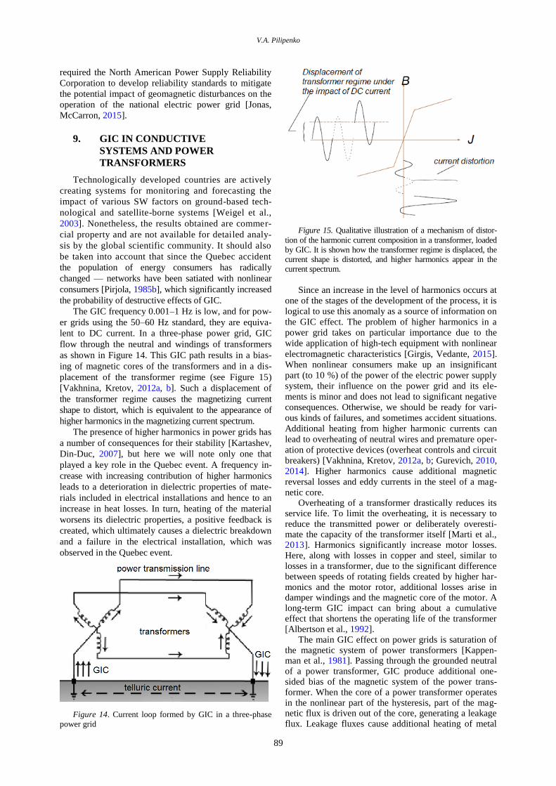
V.A. Pilipenko
89
required the North American Power Supply Reliability
Corporation to develop reliability standards to mitigate
the potential impact of geomagnetic disturbances on the
operation of the national electric power grid [Jonas,
McCarron, 2015].
9. GIC IN CONDUCTIVE
SYSTEMS AND POWER
TRANSFORMERS
Technologically developed countries are actively
creating systems for monitoring and forecasting the
impact of various SW factors on ground-based tech-
nological and satellite-borne systems [Weigel et al.,
2003]. Nonetheless, the results obtained are commer-
cial property and are not available for detailed analy-
sis by the global scientific community. It should also
be taken into account that since the Quebec accident
the population of energy consumers has radically
changed — networks have been satiated with nonlinear
consumers [Pirjola, 1985b], which significantly increased
the probability of destructive effects of GIC.
The GIC frequency 0.001–1 Hz is low, and for pow-
er grids using the 50–60 Hz standard, they are equiva-
lent to DC current. In a three-phase power grid, GIC
flow through the neutral and windings of transformers
as shown in Figure 14. This GIC path results in a bias-
ing of magnetic cores of the transformers and in a dis-
placement of the transformer regime (see Figure 15)
[Vakhnina, Kretov, 2012a, b]. Such a displacement of
the transformer regime causes the magnetizing current
shape to distort, which is equivalent to the appearance of
higher harmonics in the magnetizing current spectrum.
The presence of higher harmonics in power grids has
a number of consequences for their stability [Kartashev,
Din-Duc, 2007], but here we will note only one that
played a key role in the Quebec event. A frequency in-
crease with increasing contribution of higher harmonics
leads to a deterioration in dielectric properties of mate-
rials included in electrical installations and hence to an
increase in heat losses. In turn, heating of the material
worsens its dielectric properties, a positive feedback is
created, which ultimately causes a dielectric breakdown
and a failure in the electrical installation, which was
observed in the Quebec event.
Figure 14. Current loop formed by GIC in a three-phase
power grid
Figure 15. Qualitative illustration of a mechanism of distor-
tion of the harmonic current composition in a transformer, loaded
by GIC. It is shown how the transformer regime is displaced, the
current shape is distorted, and higher harmonics appear in the
current spectrum.
Since an increase in the level of harmonics occurs at
one of the stages of the development of the process, it is
logical to use this anomaly as a source of information on
the GIC effect. The problem of higher harmonics in a
power grid takes on particular importance due to the
wide application of high-tech equipment with nonlinear
electromagnetic characteristics [Girgis, Vedante, 2015].
When nonlinear consumers make up an insignificant
part (to 10 %) of the power of the electric power supply
system, their influence on the power grid and its ele-
ments is minor and does not lead to significant negative
consequences. Otherwise, we should be ready for vari-
ous kinds of failures, and sometimes accident situations.
Additional heating from higher harmonic currents can
lead to overheating of neutral wires and premature oper-
ation of protective devices (overheat controls and circuit
breakers) [Vakhnina, Kretov, 2012a, b; Gurevich, 2010,
2014]. Higher harmonics cause additional magnetic
reversal losses and eddy currents in the steel of a mag-
netic core. Overheating of a transformer drastically reduces its
service life. To limit the overheating, it is necessary to reduce the transmitted power or deliberately overesti-mate the capacity of the transformer itself [Marti et al., 2013]. Harmonics significantly increase motor losses. Here, along with losses in copper and steel, similar to losses in a transformer, due to the significant difference between speeds of rotating fields created by higher har-monics and the motor rotor, additional losses arise in damper windings and the magnetic core of the motor. A long-term GIC impact can bring about a cumulative effect that shortens the operating life of the transformer [Albertson et al., 1992].
The main GIC effect on power grids is saturation of the magnetic system of power transformers [Kappen-man et al., 1981]. Passing through the grounded neutral of a power transformer, GIC produce additional one-sided bias of the magnetic system of the power trans-former. When the core of a power transformer operates in the nonlinear part of the hysteresis, part of the mag-netic flux is driven out of the core, generating a leakage flux. Leakage fluxes cause additional heating of metal
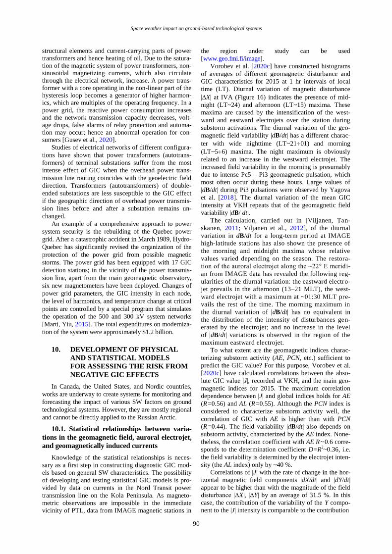
Space weather impact on ground-based technological systems
90
structural elements and current-carrying parts of power transformers and hence heating of oil. Due to the satura-tion of the magnetic system of power transformers, non-sinusoidal magnetizing currents, which also circulate through the electrical network, increase. A power trans-former with a core operating in the non-linear part of the hysteresis loop becomes a generator of higher harmon-ics, which are multiples of the operating frequency. In a power grid, the reactive power consumption increases and the network transmission capacity decreases, volt-age drops, false alarms of relay protection and automa-tion may occur; hence an abnormal operation for con-sumers [Gusev et al., 2020].
Studies of electrical networks of different configura-
tions have shown that power transformers (autotrans-
formers) of terminal substations suffer from the most
intense effect of GIC when the overhead power trans-
mission line routing coincides with the geoelectric field
direction. Transformers (autotransformers) of double-
ended substations are less susceptible to the GIC effect
if the geographic direction of overhead power transmis-
sion lines before and after a substation remains un-
changed.
An example of a comprehensive approach to power
system security is the rebuilding of the Quebec power
grid. After a catastrophic accident in March 1989, Hydro-
Quebec has significantly revised the organization of the
protection of the power grid from possible magnetic
storms. The power grid has been equipped with 17 GIC
detection stations; in the vicinity of the power transmis-
sion line, apart from the main geomagnetic observatory,
six new magnetometers have been deployed. Changes of
power grid parameters, the GIC intensity in each node,
the level of harmonics, and temperature change at critical
points are controlled by a special program that simulates
the operation of the 500 and 300 kV system networks
[Marti, Yiu, 2015]. The total expenditures on moderniza-
tion of the system were approximately $1.2 billion.
10. DEVELOPMENT OF PHYSICAL
AND STATISTICAL MODELS
FOR ASSESSING THE RISK FROM
NEGATIVE GIC EFFECTS
In Canada, the United States, and Nordic countries,
works are underway to create systems for monitoring and
forecasting the impact of various SW factors on ground
technological systems. However, they are mostly regional
and cannot be directly applied to the Russian Arctic.
10.1. Statistical relationships between varia-
tions in the geomagnetic field, auroral electrojet,
and geomagnetically induced currents
Knowledge of the statistical relationships is neces-
sary as a first step in constructing diagnostic GIC mod-
els based on general SW characteristics. The possibility
of developing and testing statistical GIC models is pro-
vided by data on currents in the Nord Transit power
transmission line on the Kola Peninsula. As magneto-
metric observations are impossible in the immediate
vicinity of PTL, data from IMAGE magnetic stations in
the region under study can be used
[www.geo.fmi.fi/image].
Vorobev et al. [2020c] have constructed histograms
of averages of different geomagnetic disturbance and
GIC characteristics for 2015 at 1 hr intervals of local
time (LT). Diurnal variation of magnetic disturbance
|X| at IVA (Figure 16) indicates the presence of mid-
night (LT~24) and afternoon (LT~15) maxima. These
maxima are caused by the intensification of the west-
ward and eastward electrojets over the station during
substorm activations. The diurnal variation of the geo-
magnetic field variability |dB/dt| has a different charac-
ter with wide nighttime (LT~2101) and morning
(LT~56) maxima. The night maximum is obviously
related to an increase in the westward electrojet. The
increased field variability in the morning is presumably
due to intense Pc5 – Pi3 geomagnetic pulsation, which
most often occur during these hours. Large values of
|dB/dt| during Pi3 pulsations were observed by Yagova
et al. [2018]. The diurnal variation of the mean GIC
intensity at VKH repeats that of the geomagnetic field
variability |dB/ dt|.
The calculation, carried out in [Viljanen, Tan-
skanen, 2011; Viljanen et al., 2012], of the diurnal
variation in dB/dt for a long-term period at IMAGE
high-latitude stations has also shown the presence of
the morning and midnight maxima whose relative
values varied depending on the season. The restora-
tion of the auroral electrojet along the ~22° E merid i-
an from IMAGE data has revealed the following reg-
ularities of the diurnal variation: the eastward electro-
jet prevails in the afternoon (13–21 MLT), the west-
ward electrojet with a maximum at ~01:30 MLT pre-
vails the rest of the time. The morning maximum in
the diurnal variation of |dB/dt| has no equivalent in
the distribution of the intensity of disturbances gen-
erated by the electrojet; and no increase in the level
of |dB/dt| variations is observed in the region of the
maximum eastward electrojet.
To what extent are the geomagnetic indices charac-
terizing substorm activity (AE, PCN, etc.) sufficient to
predict the GIC value? For this purpose, Vorobev et al.
[2020c] have calculated correlations between the abso-
lute GIC value |J|, recorded at VKH, and the main geo-
magnetic indices for 2015. The maximum correlation
dependence between |J| and global indices holds for AE
(R=0.56) and AL (R=0.55). Although the PCN index is
considered to characterize substorm activity well, the
correlation of GIC with AE is higher than with PCN
(R=0.44). The field variability |dB/dt| also depends on
substorm activity, characterized by the AE index. None-
theless, the correlation coefficient with AE R~0.6 corre-
sponds to the determination coefficient D=R2~0.36, i.e.
the field variability is determined by the electrojet inten-
sity (the AL index) only by ~40 %.
Correlations of |J| with the rate of change in the hor-
izontal magnetic field components |dX/dt| and |dY/dt|
appear to be higher than with the magnitude of the field
disturbance |ΔX|, |ΔY| by an average of 31.5 %. In this
case, the contribution of the variability of the Y compo-
nent to the |J| intensity is comparable to the contribution
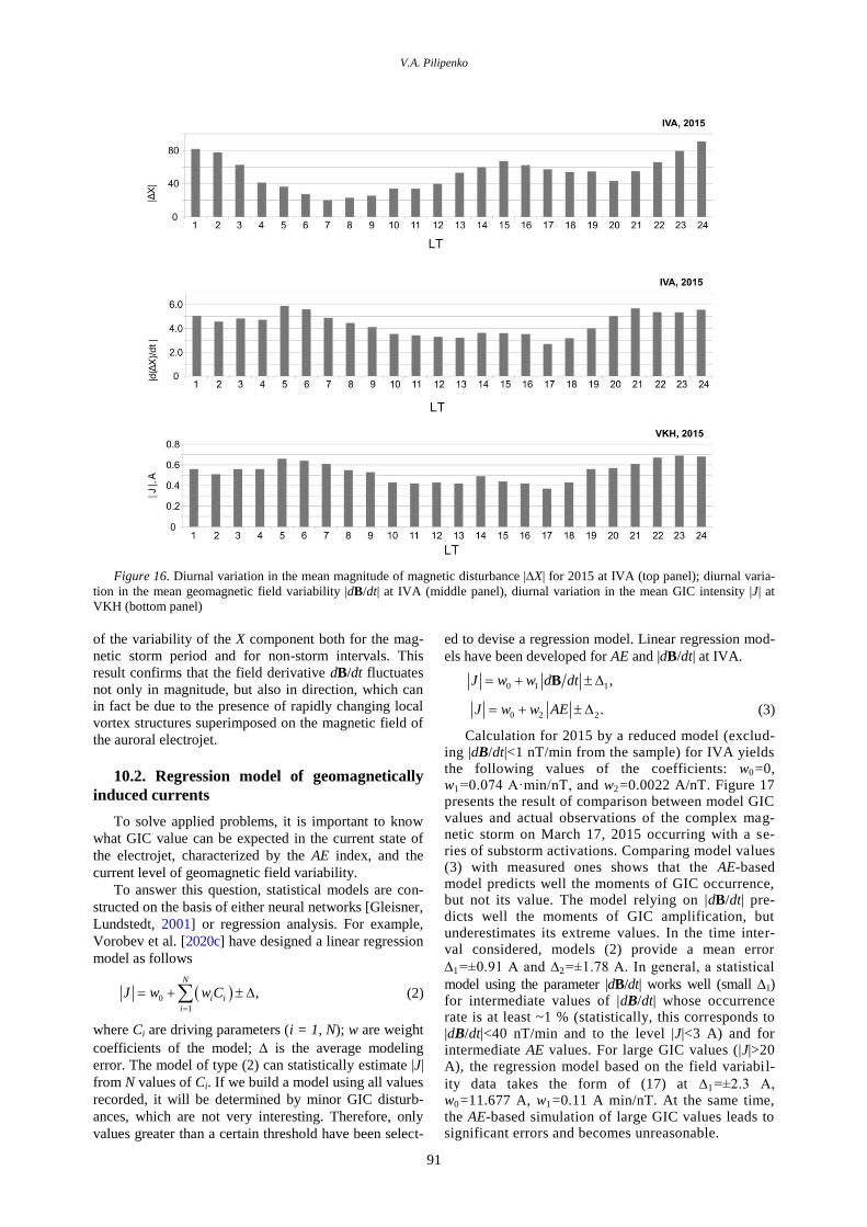
V.A. Pilipenko
91
Figure 16. Diurnal variation in the mean magnitude of magnetic disturbance |X| for 2015 at IVA (top panel); diurnal varia-
tion in the mean geomagnetic field variability |dB/dt| at IVA (middle panel), diurnal variation in the mean GIC intensity |J| at
VKH (bottom panel)
of the variability of the X component both for the mag-
netic storm period and for non-storm intervals. This
result confirms that the field derivative dB/dt fluctuates
not only in magnitude, but also in direction, which can
in fact be due to the presence of rapidly changing local
vortex structures superimposed on the magnetic field of
the auroral electrojet.
10.2. Regression model of geomagnetically
induced currents
To solve applied problems, it is important to know
what GIC value can be expected in the current state of
the electrojet, characterized by the AE index, and the
current level of geomagnetic field variability.
To answer this question, statistical models are con-
structed on the basis of either neural networks [Gleisner,
Lundstedt, 2001] or regression analysis. For example,
Vorobev et al. [2020c] have designed a linear regression
model as follows
0
1
,N
i i
i
J w w C
(2)
where Ci are driving parameters (i = 1, N); w are weight
coefficients of the model; is the average modeling
error. The model of type (2) can statistically estimate |J|
from N values of Ci. If we build a model using all values
recorded, it will be determined by minor GIC disturb-
ances, which are not very interesting. Therefore, only
values greater than a certain threshold have been select-
ed to devise a regression model. Linear regression mod-
els have been developed for AE and |dB/dt| at IVA.
0 1 1,J w w d dt B
0 2 2 .J w w AE (3)
Calculation for 2015 by a reduced model (exclud-ing |dB/dt|<1 nT/min from the sample) for IVA yields the following values of the coefficients: w0=0, w1=0.074 A·min/nT, and w2=0.0022 A/nT. Figure 17 presents the result of comparison between model GIC values and actual observations of the complex mag-netic storm on March 17, 2015 occurring with a se-ries of substorm activations. Comparing model values (3) with measured ones shows that the AE-based model predicts well the moments of GIC occurrence, but not its value. The model relying on |dB/dt| pre-dicts well the moments of GIC amplification, but underestimates its extreme values. In the time inter-val considered, models (2) provide a mean error
1=±0.91 A and 2=±1.78 A. In general, a statistical
model using the parameter |dB/dt| works well (small 1) for intermediate values of |dB/dt| whose occurrence rate is at least ~1 % (statistically, this corresponds to |dB/dt|<40 nT/min and to the level |J|<3 A) and for intermediate AE values. For large GIC values (|J|>20 A), the regression model based on the field variabil-
ity data takes the form of (17) at 1=±2.3 A, w0=11.677 A, w1=0.11 A min/nT. At the same time, the AE-based simulation of large GIC values leads to significant errors and becomes unreasonable.
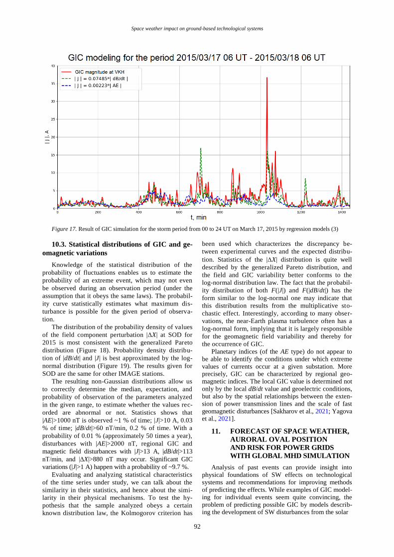
Space weather impact on ground-based technological systems
92
Figure 17. Result of GIC simulation for the storm period from 00 to 24 UT on March 17, 2015 by regression models (3)
10.3. Statistical distributions of GIC and ge-
omagnetic variations
Knowledge of the statistical distribution of the
probability of fluctuations enables us to estimate the
probability of an extreme event, which may not even
be observed during an observation period (under the
assumption that it obeys the same laws). The probabil-
ity curve statistically estimates what maximum dis-
turbance is possible for the given period of observa-
tion.
The distribution of the probability density of values
of the field component perturbation |ΔX| at SOD for
2015 is most consistent with the generalized Pareto
distribution (Figure 18). Probability density distribu-
tion of |dB/dt| and |J| is best approximated by the log-
normal distribution (Figure 19). The results given for
SOD are the same for other IMAGE stations.
The resulting non-Gaussian distributions allow us
to correctly determine the median, expectation, and
probability of observation of the parameters analyzed
in the given range, to estimate whether the values rec-
orded are abnormal or not. Statistics shows that
|AE|>1000 nT is observed ~1 % of time; |J|>10 A, 0.03
% of time; |dB/dt|>60 nT/min, 0.2 % of time. With a
probability of 0.01 % (approximately 50 times a year),
disturbances with |AE|>2000 nT, regional GIC and
magnetic field disturbances with |J|>13 A, |dB/dt|>113
nT/min, and |ΔX|>880 nT may occur. Significant GIC
variations (|J|>1 A) happen with a probability of ~9.7 %.
Evaluating and analyzing statistical characteristics
of the time series under study, we can talk about the
similarity in their statistics, and hence about the simi-
larity in their physical mechanisms. To test the hy-
pothesis that the sample analyzed obeys a certain
known distribution law, the Kolmogorov criterion has
been used which characterizes the discrepancy be-
tween experimental curves and the expected distribu-
tion. Statistics of the |X| distribution is quite well
described by the generalized Pareto distribution, and
the field and GIC variability better conforms to the
log-normal distribution law. The fact that the probabil-
ity distribution of both F(|J|) and F(|dB/dt|) has the
form similar to the log-normal one may indicate that
this distribution results from the multiplicative sto-
chastic effect. Interestingly, according to many obser-
vations, the near-Earth plasma turbulence often has a
log-normal form, implying that it is largely responsible
for the geomagnetic field variability and thereby for
the occurrence of GIC.
Planetary indices (of the AE type) do not appear to be able to identify the conditions under which extreme values of currents occur at a given substation. More precisely, GIC can be characterized by regional geo-magnetic indices. The local GIC value is determined not only by the local dB/dt value and geoelectric conditions, but also by the spatial relationships between the exten-sion of power transmission lines and the scale of fast geomagnetic disturbances [Sakharov et al., 2021; Yagova et al., 2021].
11. FORECAST OF SPACE WEATHER,
AURORAL OVAL POSITION
AND RISK FOR POWER GRIDS
WITH GLOBAL MHD SIMULATION
Analysis of past events can provide insight into physical foundations of SW effects on technological systems and recommendations for improving methods of predicting the effects. While examples of GIC model-ing for individual events seem quite convincing, the problem of predicting possible GIC by models describ-ing the development of SW disturbances from the solar
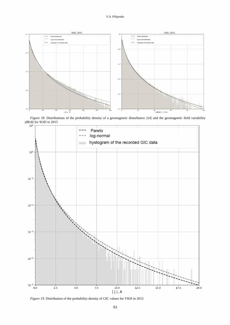
V.A. Pilipenko
93
Figure 18. Distributions of the probability density of a geomagnetic disturbance |X| and the geomagnetic field variability
|dB/dt| for SOD in 2015
Figure 19. Distribution of the probability density of GIC values for VKH in 2015
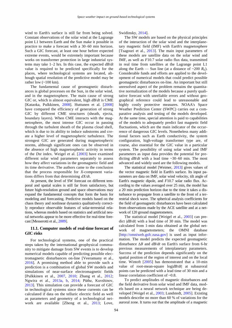
Space weather impact on ground-based technological systems
94
wind to Earth's surface is still far from being solved.
Constant observations of the solar wind at the Lagrange
point L1 between Earth and the Sun make it possible in
practice to make a forecast with a 30–60 min horizon.
Such a GIC forecast, at least one hour before expected
extreme events, would be extremely important because
works on transformer protection in large industrial sys-
tems may take 1–2 hrs. In this case, the expected dB/dt
value is required to be predicted specifically for the
places, where technological systems are located, alt-
hough spatial resolution of the predictive model may be
rather low (~100 km).
The fundamental cause of geomagnetic disturb-
ances is global processes on the Sun, in the solar wind,
and in the magnetosphere. The main cause of strong
GIC or, which is almost equivalent, high dB/dt is CME
[Kataoka, Pulkkinen, 2008]. Huttunen et al. [2008]
have compared the efficiency of generation of strong
GIC by different CME structures (sheath, ejecta,
boundary layers). When CME interacts with the mag-
netosphere, the most intense GIC occur in passing
through the turbulent sheath of the plasma cloud shell,
which is due to its ability to induce substorms and cre-
ate a higher level of magnetospheric turbulence. The
strongest GIC are generated during magnetospheric
storms, although significant ones can be observed in
the absence of high magnetospheric activity in terms
of the Dst index. Weigel et al. [2003] have examined
different solar wind parameters separately to assess
how they affect variations in the geomagnetic field and
its time derivative. The authors came to the conclusion
that the process responsible for X-component varia-
tions differs from that determining dX/dt.
At present, the level of SW forecast on different tem-
poral and spatial scales is still far from satisfactory, but
future high-resolution ground and space observations may
expand the fundamental concepts that form the basis for
modeling and forecasting. Predictive models based on the
chaos theory and nonlinear dynamics qualitatively correct-
ly reproduce observable features of solar-terrestrial rela-
tions, whereas models based on statistics and artificial neu-
ral networks appear to be more effective for real-time fore-
cast [Messerotti et al., 2009].
11.1. Computer models of real-time forecast of
GIC risks
For technological systems, one of the practical
steps taken by the international geophysical commu-
nity to mitigate damage from SW events is to develop
numerical models capable of predicting possible elec-
tromagnetic disturbances on-line [Veeramany et al.,
2016]. A promising method able to provide such a
prediction is a combination of global SW models and
simulations of near-surface electromagnetic fields
[Pulkkinen et al., 2007, 2010; Zhang et al., 2012;
Ngwira et al., 2013a, b, 2014; Püthe, Kuvshinov,
2013]. This simulation can provide a forecast of GIC
in technological systems since these currents can be
calculated if data on the telluric electric field as well
as parameters and geometry of a technological net-
work are available [Zheng et al., 2013; Love,
Swidinsky, 2014].
The SW models are based on the physical principles
of the interaction of the solar wind and the interplane-
tary magnetic field (IMF) with Earth's magnetosphere
[Tsagouri et al., 2013]. The main input parameters of
these models are satellite data on the solar wind and
IMF, as well as F10.7 solar radio flux data, transmitted
in real time from satellites at the Lagrange point L1
along the Earth — Sun line (at a distance of ~200 RE).
Considerable funds and efforts are applied to the devel-
opment of numerical models that could predict possible
geomagnetic disturbances on-line. An important but still
unresolved aspect of the problem remains the quantita-
tive normalization of the models because a purely quali-
tative forecast with unreliable errors and without geo-
graphical reference could lead to unreasonable and
highly costly protective measures. NOAA's Space
Weather Prediction Center (SWPC) carries out a com-
parative analysis and testing of the models developed.
At the same time, special attention is paid to capabilities
of the models to adequately predict fast magnetic field
fluctuations, which are the main indicator of the occur-
rence of dangerous GIC levels. Nonetheless many addi-
tional factors such as Earth conductivity, the system
configuration, high-voltage transformer type are, of
course, also essential for the GIC value in a particular
system. The possibility of using solar wind and IMF
parameters as input data provides the potential for pre-
dicting dB/dt with a lead time ~30–60 min. The most
advanced and widely used are the following models.
The statistical model [Weimer, 2013] gives values of
the vector magnetic field in Earth's surface. Its input pa-
rameters are data on IMF, solar wind velocity, tilt angle of
Earth's magnetic dipole, and F10.7 solar radio flux. Ac-
cording to the values averaged over 25 min, the model has
a 20 min prediction horizon due to the time it takes a dis-
turbance to propagate from a satellite to the front of a ter-
restrial shock wave. The spherical analysis coefficients for
the field of geomagnetic disturbances have been calculated
from observations made by the ACE satellite and at a net-
work of 120 ground magnetometers.
The statistical model [Weigel et al., 2003] can pre-
dict |dB/dt| with a lead time of 30 min. The model was
calculated from 1-min data obtained at the global net-
work of magnetometers; the OMNI database
[http://omniweb.gsfc.nasa.gov] is used as input infor-
mation. The model predicts the expected geomagnetic
disturbance В and dB/dt on Earth's surface from 6-hr
previous measurements of interplanetary parameters.
Success of the prediction depends significantly on the
spatial position of the region of interest and on the local
time. Wintoft [2005] has demonstrated that a 10-min
value of root-mean-square log|dB/dt| at subauroral
points can be predicted with a lead time of 30 min and a
linear correlation coefficient of ~0.8.
To predict amplitudes of magnetic disturbances and
the field derivative from solar wind and IMF data, mod-
els based on a neural network technique are being de-
veloped [Weigel et al., 2003; Lundstedt, 2005]. Existing
models describe no more than 60 % of variations for the
auroral zone. It turns out that the amplitude of a magnetic
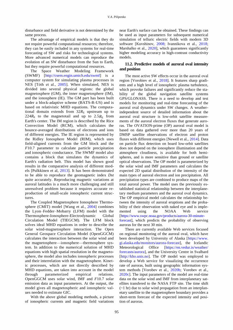
V.A. Pilipenko
95
disturbance and field derivative is not determined by the
same process.
The advantage of empirical models is that they do
not require powerful computational resources; therefore,
they can be easily included in any systems for real-time
forecasting of SW and risks for technological systems.
More advanced numerical models can reproduce the
evolution of an SW disturbance from the Sun to Earth,
but they require powerful computational resources.
The Space Weather Modeling Framework
(SWMF) [http://csem.engin.umich.edu/swmf] is a
computer system for simulating plasma processes in
NES [Tόth et al., 2005]. When simulated, NES is
divided into several physical regions: the global
magnetosphere (GM), the inner magnetosphere (IM),
and the ionosphere (IE). The GM part has been built
under a block-adaptive scheme (BATS-R-US) and is
based on relativistic MHD equations. The computa-
tional domain extends from 32RE upstream up to
224RE to the magnetotail and up to 2.5RE from
Earth's center. The IM region is described by the Rice
Convection Model (RCM), which calculates the
bounce-averaged distributions of electrons and ions
of different energies. The IE region is represented by
the Ridley Ionosphere Model (RIM), which uses
field-aligned currents from the GM block and the
F10.7 parameter to calculate particle precipitation
and ionospheric conductance. The SWMF model also
contains a block that simulates the dynamics of
Earth's radiation belt. This model has shown good
results in the comparative analysis of different mod-
els [Pulkkinen et al, 2013]. It has been demonstrated
to be able to reproduce the geomagnetic index Dst
quite accurately. Reproducing magnetic variations at
auroral latitudes is a much more challenging and still
unresolved problem because it requires accurate re-
production of small-scale ionospheric current struc-
tures.
The Coupled Magnetosphere Ionosphere Thermo-
sphere (CMIT) model [Wang et al., 2004] combines
the Lyon–Fedder–Mobarry (LFM) model with the
Thermosphere-Ionosphere-Electrodynamic Global
Circulation Model (TIEGCM). The LFM block
solves ideal MHD equations in order to describe the
solar wind-magnetosphere interaction. The Open
General Geospace Circulation Model (OpenGGCM)
calculates the interaction between the solar wind and
the magnetosphere—ionosphere—thermosphere sys-
tem. In addition to the numerical solution of MHD
equations with high spatial resolution in the magneto-
sphere, the model also includes ionospheric processes
and their interrelation with the magnetosphere. Kinet-
ic processes, which are not directly described by
MHD equations, are taken into account in the model
through parameterized empirical relations.
OpenGGCM uses solar wind, IMF and F10.7 solar
emission data as input parameters. At the output, the
model gives all magnetospheric and ionospheric val-
ues needed to estimate GIC.
With the above global modeling methods, a picture
of ionospheric currents and magnetic field variations
near Earth's surface can be obtained. These findings can
be used as input parameters for subsequent numerical
simulation of telluric electric fields with modern 3D
software [Kuvshinov, 2008; Ivannikova et al., 2018;
Marshalko et al., 2020], which guarantees significantly
higher modeling accuracy in high-contrast conductivity
models.
11.2. Predictive models of auroral oval intensity
and position
The most active SW effects occur in the auroral oval
region [Vorobiev et al., 2018]. It features sharp gradi-
ents and a high level of ionospheric plasma turbulence,
which provoke failures and significantly reduce the sta-
bility of the global navigation satellite systems
GPS/GLONASS. There is a need to develop and test
models for monitoring and real-time forecasting of the
auroral oval dynamics under SW changes. A weather-
independent source of detailed information about the
auroral oval structure is low-orbit satellite measure-
ments of the auroral electron fluxes that generate auro-
ras. The OVATION-prime (OP) auroral oval model is
based on data gathered over more than 20 years of
DMSP satellite observations of electron and proton
fluxes with different energies [Newell et al., 2014]. Data
on particle flux detection on board low-orbit satellites
does not depend on the ionosphere illumination and the
atmosphere cloudiness, is available for both hemi-
spheres, and is more sensitive than ground or satellite
optical observations. The OP model is parameterized by
the solar wind and IMF parameters and calculates the
expected 2D spatial distribution of the intensity of the
main types of auroral electron and ion precipitation. All
precipitation types are combined to produce maps of the
total auroral power. The model uses the previously es-
tablished statistical relationship between the interplane-
tary medium parameters and the auroral oval dynamics.
The OP empirical model calculates the relationship be-
tween the intensity of auroral eruptions and the proba-
bility of their observation with naked eye and is imple-
mented using the NOAA Web service
[https://www.swpc.noaa.gov/products/aurora-30-minute-
forecast], which predicts the probability of observing
auroras for the next 30 min.
There are currently available Web services focused
on regional monitoring of the auroral oval, which have
been developed by University of Alaska [https://www.
gi.alaska.edu/monitors/aurora-forecast], the Icelandic
Meteorological Office [https://en.vedur.is/weather/
forecasts/aurora], and the University Centre in Svalbard
[http://kho.unis.no]. The OP model was employed to
develop a Web service for visualizing the occurrence
rate of auroras, built using geographic information sys-
tem methods [Vorobev et al., 2020b; Vorobev et al.,
2020c]. The input parameters of the model are real-time
data on the solar wind and IMF from interplanetary sat-
ellites transfered to the NASA FTP site. The time shift
(~1 hr) due to solar wind propagation from an interplan-
etary satellite to the magnetosphere boundary provides a
short-term forecast of the expected intensity and posi-
tion of auroras.
Space weather impact on ground-based technological systems
96
12. CONCLUSION: OBJECTIVES
OF FURTHER RESEARCH
To date, space geophysics has reached a level that
allows us to raise the question about real SW forecast.
The objective of SW research is, on the one hand, to
identify the relationships between solar activity and
processes occurring in the interplanetary space, Earth's
magnetosphere, ionosphere, and atmosphere; on the
other hand, to analyze the influence of these processes
on technogenic and biological systems. This problem is
becoming more and more urgent since modern high-
tech systems, especially space-borne ones, are very sen-
sitive to the effects of electromagnetic fields and radia-
tion. Despite the large arsenal of modern space geo-
physics — solar telescopes, space stations between
Earth and the Sun, hundreds of satellites in different
orbits, networks of ground radars and magnetometers,
etc. — the problem of monitoring and forecasting the
state of NES has not been reduced to purely engineer-
ing; many fundamental questions remain unresolved.
Unlike hurricanes and storms that have a regional ef-
fect and are quite successfully predicted 2–3 days in
advance, SW disturbances can span continents and de-
velop within minutes after the initial disturbances have
been detected in the solar wind. Although visual regis-
tration of solar flares and coronal mass ejections is
available several days before the occurrence of geo-
magnetic disturbances, only a small part of solar ejec-
tions pose a threat of magnetic storms and GIC. Exactly
what solar events cause intense GIC to occur remains an
unresolved and actively studied issue. The objective of
forecasting GIC is not reduced to the forecasting of
magnetic storms. The model required for assessing the
influence of geomagnetic activity on technological sys-
tems in arctic and subarctic latitudes should describe not
only the dynamics of the large-scale magnetospheric-
ionospheric current system, but also the rapidly varying
localized field-aligned currents sporadically arising in it.
Having a calculated pattern of telluric fields, we can
make an engineering calculation of GIC in a given tech-
nological system with a known geometry and structure.
Estimating possible effects for each specific system is a
separate task. Then, by calculating the response of po-
tentials along a given branch of a pipeline or a power
grid to GIC, engineers can fully imagine the behavior of
cathodic protection during magnetic storms and identify
weak elements of the grid. Operators can use the real-
time forecast of possible critical levels of GIC to reduce
the risk of catastrophic consequences (load reduction,
capacitive protection system connection, etc.). Infor-
mation about GIC is important not only from a practical
point of view, but also from a general scientific point of
view as GIC is an important element of the influence of
solar activity on the magnetosphere — ionosphere system.
The most active effects of geomagnetic disturbances
occur at auroral latitudes; therefore, in Nordic countries
since the 1970s the GIC influence on ground technolog-
ical systems and possible measures to reduce negative
consequences have been studied. Even countries located
at low latitudes are concerned about the possible impact
of GIC on technological systems. These factors pose a
particular threat to the safe operation of technological
systems in the Russian Arctic zone, since the Russian
Federation has the longest oil and gas pipelines, power
transmission lines, and main traffic arteries [Sushko,
Kosykh, 2013]. Calculation of possible GIC levels dur-
ing typical and extreme magnetic storms, which can be
used by network operators to take the necessary
measures to reduce the risk of catastrophic consequenc-
es, is a very urgent task. Despite the exceptional im-
portance of such research, the Russian academic com-
munity is practically not engaged in such tasks, and
manufacturing companies of the Russian Federation at
the moment do not show any interest in sustainable
management of technological systems. The level and
scope of domestic research in this area clearly lag be-
hind the works carried out in advanced countries. The
domestic reference documentation still does not take
into account the GIC impact on electric power systems
and the reliability of electrical equipment, although the
task of accounting for potentially dangerous geomagnet-
ic disturbances is relevant specifically for Russia due to
the great length of power networks and pipelines at high
latitudes. In addition, unlike Nordic countries and Can-
ada, the auroral regions of the Russian Federation do not
have a sufficiently dense network of magnetic stations.
In many cases, information on GIC is the property of
commercial industrial companies and is not available to
the global scientific community for in-depth analysis.
To clarify laws of manifestations of the impact of
geomagnetic disturbances on the operation of railway
automation and to search for ways to limit the impact, it
is reasonable to continue the study of anomalies in the
sections of railway networks located primarily in the
Arctic and subarctic zones. While the maximum GIC
values recorded in railway conductors (>1 A) are not
extremely high, the intense operation of expressway and
high risks require careful attention to the impact of ge-
omagnetic disturbances.
The need to develop a domestic model capable of es-
timating the SW parameters critical for technological
systems has become urgent. The key output parameters
of the model are statistical maps of magnetic field and
GIC variability during magnetic storms and substorms,
parameterized using various sets of solar wind and in-
terplanetary magnetic field parameters, and geomagnet-
ic indices. Statistical maps of GIC are input parameters
for calculating induced currents in given technological
systems. Synthetic models will provide an opportuni-
ty to identify weak elements of the technological net-
work in terms of GIC and to predict critical GIC levels
(for 0.5–1 hr), thereby enabling operators to take the
necessary measures to reduce the risk of catastrophic
consequences. It is also necessary to develop a global
statistical model of alternating magnetic field over the
ionosphere, electric currents flowing between the mag-
netosphere and the ionosphere along the geomagnetic
field lines (field-aligned currents), a numerical model of
electric currents in the ionosphere, a model of distribu-
tion of the rate of change of the geomagnetic field on
Earth's surface and associated variations in the telluric
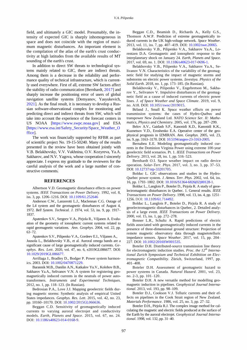
V.A. Pilipenko
97
field, and ultimately a GIC model. Presumably, the in-
tensity of expected GIC is sharply inhomogeneous in
space and does not coincide with the region of maxi-
mum magnetic disturbances. An important element is
the compilation of the atlas of the earth's crust conduc-
tivity at high latitudes from the available results of MT
sounding of the earth's crust.
In addition to direct SW threats to technological sys-
tems mainly related to GIC, there are indirect threats.
Among them is a decrease in the reliability and perfor-
mance quality of technical infrastructure, which is current-
ly used everywhere. First of all, extreme SW factors affect
the stability of radio communication [Bernhardt, 2017] and
sharply increase the positioning error of users of global
navigation satellite systems [Demyanov, Yasyukevich,
2021]. As the final result, it is necessary to develop a Rus-
sian software-observational complex for monitoring and
predicting direct and indirect threats from SW, which will
take into account the experience of the forecast centers in
US NOAA [https://www.swpc.noaa.gov] and ESA
[https://www.esa.int/Safety_Security/Space_Weather_O
ffice].
The work was financially supported by RFBR as part
of scientific project No. 19-15-50240. Many of the results
presented in the review have been obtained jointly with
V.B. Belakhovsky, V.V. Vakhnina, O.V. Kozyreva, Ya.A.
Sakharov, and N.V. Yagova, whose cooperation I sincerely
appreciate. I express my gratitude to the reviewers for the
careful analysis of the work and a large number of con-
structive comments.
REFERENCES
Albertson V.D. Geomagnetic disturbance effects on power
systems. IEEE Transactions on Power Delivery. 1992, vol. 8,
iss. 3, pp. 1206–1216. DOI: 10.1109/61.252646
Anderson C.W., Lanzerotti L.J., Maclennan C.G. Outage of
the L4 system and the geomagnetic disturbances of August 4,
1972. Bell System. Technical. J. 1974, vol. 53, iss. 9, pp. 1917–
1837.
Apatenkov S.V., Sergeev V.A., Pirjola R., Viljanen A. Evalu-
ation of the geometry of ionospheric current systems related to
rapid geomagnetic variations. Ann. Geophys. 2004, vol. 22, pp.
63–72.
Apatenkov S.V., Pilipenko V.A., Gordeev E.I., Viljanen A.,
Juusola L., Belakhovsky V.B., et al. Auroral omega bands are a
significant cause of large geomagnetically induced currents. Ge-
ophys. Res. Lett. 2020, vol. 47, no. 6, e2019GL086677. DOI:
10.1029/2019GL086677.
Arrillaga J., Bradley D., Bodger P. Power system harmon-
ics. 2003. DOI: 10.1002/0470871229.
Barannik M.B., Danilin A.N., Katkalov Yu.V., Kolobov B.B.,
Sakharov Ya.A., Selivanov V.N. A system for registering geo-
magnetically induced currents in the neutrals of power auto-
transformers. Instruments and Experimental Techniques.
2012, no. 1, pp. 118–123. (In Russian).
Bedrosian P.A., Love J.J. Mapping geoelectric fields dur-
ing magnetic storms: Synthetic analysis of empirical United
States impedances. Geophys. Res. Lett. 2015, vol. 42, no. 23,
pp. 10160–10170. DOI: 10.1002/2015GL066636.
Beggan C.D. Sensitivity of geomagnetically induced
currents to varying auroral electrojet and conductivity
models. Earth, Planets and Space. 2015, vol. 67, no. 24.
DOI: 10.1186/s40623-014-0168-9.
Beggan C.D., Beamish D., Richards A., Kelly G.S.,
Thomson A.W.P. Prediction of extreme geomagnetically in-
duced currents in the UK high-voltage network. Space Weather.
2013, vol. 11, iss. 7, pp. 407–419. DOI: 10.1002/swe.20065.
Belakhovsky V.B., Pilipenko V.A., Sakharov Ya.A., Lo-
rentzen D.A. Geomagnetic and ionospheric response to the
interplanetary shock on January 24. Earth, Planets and Space.
2017, vol. 69, no. 1. DOI: 10.1186/s40623-017-0696-1.
Belakhovsky V.B., Pilipenko V.A., Sakharov Ya.A., Se-
livanov V.N. Characteristics of the variability of the geomag-
netic field for studying the impact of magnetic storms and
substorms on electric power systems. Izvestiya. Physics of the
Solid Earth. 2018, no. 1, pp. 173–185. (In Russian).
Belakhovsky V., Pilipenko V., Engebretson M., Sakha-
rov Y., Selivanov V. Impulsive disturbances of the geomag-
netic field as a cause of induced currents of electric power
lines. J. of Space Weather and Space Climate. 2019, vol. 9,
no. A18. DOI: 10.1051/swsc/2019015. Béland J., Small K. Space weather effects on power
transmission systems: the cases of Hydro-Québec and
transpower New Zealand Ltd. NATO Science Ser. II: Mathe-matics, Physics and Chemistry. 2005, vol. 176, pp. 287–299.
Belov A.V., Gaidash S.P., Kanonidi K.D., Kanonidi K.K., Kuznetsov V.D., Eroshenko E.A. Operative center of the geo-
physical prognosis in IZMIRAN. Ann. Geophys. 2005, vol. 23,
iss. 9, pp. 3163–3170. DOI: 10.5194/angeo-23-3163-2005. Bernabeu E.E. Modeling geomagnetically induced cur-
rents in the Dominion Virginia Power using extreme 100-year geoelectric field scenarios. Pt. 1. IEEE Transactions on Power
Delivery. 2013, vol. 28, iss. 1, pp. 516–523. Bernhardt O.I. Space weather impact on radio device
operation. Solar-Terr. Phys. 2017, vol. 3, no. 3, pp. 37–53. DOI: 10.12737/stp-33201705.
Bolduc L. GIC observations and studies in the Hydro-Quebec power system. J. Atmos. Terr. Phys. 2002, vol. 64, iss.
16, pp. 1793–1802. DOI: 10.1016/S1364-6826(02)00128-1. Bolduc L., Langlois P., Boteler D., Pirjola R. A study of geoe-
lectromagnetic disturbances in Quebec. 1. General results. IEEE Transactions on Power Delivery. 1998, vol. 13, iss. 4, pp. 1251–
1256. DOI: 10.1109/61.714492. Bolduc L., Langlois P., Boteler D., Pirjola R. A study of
geoelectromagnetic disturbances in Quebec, 2. Detailed analy-sis of a large event. IEEE Transactions on Power Delivery.
2000, vol. 15, iss. 1, pp. 272–278. Bonner L.R., Schultz A. Rapid predictions of electric
fields associated with geomagnetically induced currents in the
presence of three-dimensional ground structure: Projection of remote magnetic observatory data through magnetotelluric
impedance tensors. Space Weather. 2017, vol. 15, pp. 204–227. DOI: 10.1002/2016SW001535.
Boteler D.H. Distributed-source transmission line theory for electromagnetic induction studies. Proc. the 12th Interna-
tional Zurich Symposium and Technical Exhibition on Elec-tromagnetic Compatibility. Zürich, Switzerland, 1997, pp.
401–408. Boteler D.H. Assessment of geomagnetic hazard to
power systems in Canada. Natural Hazard. 2001, vol. 23, no. 2-3, pp. 101–120.
Boteler D.H. A new versatile method for modelling geo-magnetic induction in pipelines. Geophysical Journal Interna-
tional. 2013, vol. 193, pp. 98–109. Boteler D.J., Cookson V.J. Telluric currents and their ef-
fects on pipelines in the Cook Strait region of New Zealand. Materials Performance. 1986, vol. 25, no. 3, pp. 27–32.
Boteler D.H., Pirjola R.J. The complex image method for cal-
culating the magnetic and electric fields produced at the surface of the Earth by the auroral electrojet. Geophysical Journal Interna-
tional. 1998, vol. 132, pp. 31–40.
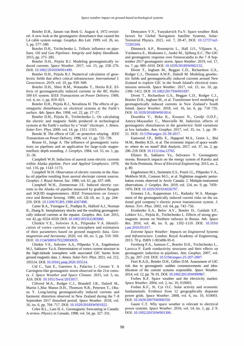
Space weather impact on ground-based technological systems
98
Boteler D.H., Jansen van Beek G. August 4, 1972 revisit-
ed: A new look at the geomagnetic disturbance that caused the
L4 cable system outage. Geophys. Res Lett. 1999, vol. 26, no.
5, pp. 577–580.
Boteler D.H., Trichtchenko L. Telluric influence on pipe-
lines. Oil and Gas Pipelines: Integrity and Safety Handbook.
2015, pp. 275–285.
Boteler D.H., Pirjola R.J. Modeling geomagnetically in-
duced currents. Space Weather. 2017, vol. 15, pp. 258–276.
DOI: 10.1002/2016SW001499.
Boteler D.H., Pirjola R.J. Numerical calculation of geoe-
lectric fields that affect critical infrastructure. International J.
Geosciences. 2019, vol. 10, pp. 930–949.
Boteler D.H., Shier R.M., Watanabe T., Horita R.E. Ef-
fects of geomagnetically induced currents in the BC Hydro
500 kV system. IEEE Transactions on Power Delivery. 1989,
vol. 4, no. 1, pp. 818–823.
Boteler D.H., Pirjola R.J., Nevalinna H. The effects of ge-
omagnetic disturbances on electrical systems at the Earth’s
surface. Adv. Space. Res. 1998, vol. 22, pp. 17–27.
Boteler D.H., Pirjola R., Trichtchenko L. On calculating
the electric and magnetic fields produced in technological
systems at the Earth’s surface by a “wide” electrojet. J. Atmos.
Solar-Terr. Phys. 2000. vol. 14. pp. 1311–1315.
Bozoki B. The effects of GIC on protective relaying. IEEE
Transactions on Power Delivery. 1996, vol. 11, pp. 725–739.
Brasse H., Junge A. The influence of geomagnetic varia-
tions on pipelines and an application for large-scale magne-
totelluric depth sounding. J. Geophys. 1984, vol. 55, no. 1, pp.
31–36.
Campbell W.H. Induction of auroral zone electric currents
within Alaska pipeline. Pure and Applied Geophysics. 1978,
vol. 116, pp. 1143–1173.
Campbell W.H. Observation of electric currents in the Alas-
ka oil pipeline resulting from auroral electrojet current sources.
Geophys. J. Royal Astron. Soc. 1980, vol. 61, pp. 437–449.
Campbell W.H., Zimmerman J.E. Induced electric cur-
rents in the Alaska oil pipeline measured by gradient fluxgate
and SQUID magnetometers. IEEE Transactions on Geosci-
ence and Remote Sensing. 1980, vol. GE-18, no. 3, pp. 244–
250. DOI: 10.1109/TGRS.1980.4307498.
Carter B.A., Yizengaw E., Pradipta R., Halford A.J., Norman
R., Zhang K. Interplanetary shocks and the resulting geomagneti-
cally induced currents at the equator. Geophys. Res. Lett. 2015,
vol. 42, pp. 6554–6559. DOI: 10.1002/2015GL065060.
Chinkin V.E., Soloviev A.A., Pilipenko V.A. Identifi-
cation of vortex currents in the ionosphere and estimation
of their parameters based on ground magnetic data. Geo-
magnetism and Aeronomy. 2020, vol. 60, no. 5, pp. 559–569.
DOI: 10.1134/S0016793220050035.
Chinkin V.E., Soloviev A.A., Pilipenko V.A., Engebretson
M.J., Sakharov Ya.A. Determination of vortex current structure in
the high-latitude ionosphere with associated GIC bursts from
ground magnetic data. J. Atmos. Solar-Terr. Phys. 2021, vol. 212,
105514. DOI: 10.1016/j.jastp.2020.105514.
Cid C., Saiz E., Guerrero A., Palacios J., Cerrato Y. A
Carrington-like geomagnetic storm observed in the 21st centu-
ry. J. Space Weather and Space Climate. 2015, vol. 5, no.
A16. DOI: 10.1051/Swsc/2015017.
Clilverd M.A., Rodger C.J., Brundell J.B., Dalzell M.,
Martin I.,Mac Manus D.H., Thomson N.R., Petersen T., Oba-
na Y. Long-lasting geomagnetically induced currents and
harmonic distortion observed in New Zealand during the 7–8
September 2017 disturbed period. Space Weather. 2018, vol.
16, iss. 6, pp. 704–717. DOI: 10.1029/2018SW001822.
Coles R.L., Lam H.-L. Geomagnetic forecasting in Canada:
A review. Physics in Canada. 1998, vol. 54, pp. 327–331.
Demyanov V.V., Yasyukevich Yu.V. Space weather: Risk
factors for Global Navigation Satellite Systems, Solar-
Terrestrial Physics. 2021, vol. 7, 28-47, DOI: 10.12737/szf-
72202104.
Dimmock A.P., Rosenqvist L., Hall J.O., Viljanen A.,
Yordanova E., Honkonen I., André M., Sjöberg E.C. The GIC
and geomagnetic response over Fennoscandia to the 7–8 Sep-
tember 2017 geomagnetic storm. Space Weather. 2019, vol. 17,
iss. 7, pp. 989–1010. DOI: 10.1029/2018SW002132.
Divett T., Ingham M., Beggan C.D., Richardson G.S.,
Rodger C.J., Thomson A.W.P., Dalzell M. Modeling geoelec-
tric fields and geomagnetically induced currents around New
Zealand to explore GIC in the South Island's electrical trans-
mission network. Space Weather. 2017, vol. 15, iss. 10, pp.
1396–1412. DOI: 10.1002/2017SW001697.
Divett T., Richardson G.S., Beggan C.D., Rodger C.J.,
Boteler D.H., Ingham M., et al. Transformer level modeling of
geomagnetically induced currents in New Zealand’s South
Island. Space Weather. 2018, vol. 16, iss. 6, pp. 718–735.
DOI: 10.1029/2018SW001814.
Doumbia V., Boka K., Kouassi N., Grodji O.D.F.,
Amory-Mazaudier C., Menvielle M. Induction effects of
geomagnetic disturbances in the geoelectric field variations
at low latitudes. Ann. Geophys. 2017, vol. 35, iss. 1, pp. 39–
51. DOI: 10.5194/angeo-35-39-2017.
Eastwood J.P., Biffis E., Hapgood M.A., Green L., Bisi
M.M., Bentley R.D., et al. The economic impact of space weath-
er: where do we stand? Risk Analysis. 2017, vol. 37, iss. 2, pp.
206–218. DOI: 10.1111/risa.12765.
Efimov B., Sakharov Ya., Selivanov V. Geomagnetic
storms. Research impacts on the energy system of Karelia and
the Kola Peninsula. News of Electrical Engineering. 2013, no. 2,
p. 80.
Engebretson M.J., Steinmetz E.S., Posch J.L., Pilipenko V.A.,
Moldwin M.B., Connors M.G., et al. Nighttime magnetic pertur-
bation events observed in Arctic Canada: 2. Multiple-instrument
observations. J. Geophys. Res. 2019, vol. 124, no. 9, pp. 7459–
7476. DOI: 10.1029/2019JA026797.
Erinmez I.A., Kappenman J.G., Radasky W.A. Manage-
ment of the geomagnetically induced current risks on the na-
tional grid company’s electric power transmission system. J.
Atmos. Terr. Phys. 2002, vol. 64, pp. 743–756.
Eroshenko E.A., Belov A.V., Boteler D., Gaidash S.P.,
Lobkov S.L., Pirjola R., Trichtchenko L. Effects of strong geo-
magnetic storms on Northern railways in Russia. Adv. Space
Res. 2010, vol. 46, iss. 9, pp. 1102–1110. DOI: 10.1016/
j.asr.2010.05.017.
Extreme Space Weather: Impacts on Engineered Systems
and Infrastructure. London: Royal Academy of Engineering,
2013. 70 p. ISBN 1-903496-95-0.
Fernberg P.A., Samson C., Boteler D.H., Trichtchenko L.,
Larocca P. Earth conductivity structures and their effects on
geomagnetic induction in pipelines. Ann. Geophys. 2007, vol.
25, pp. 207–218. DOI: 10.5194/angeo-25-207-2007.
Fiori R.A.D., Boteler D.H., Gillies D.M. Assessment of GIC
risk due to geomagnetic sudden commencements and iden-
tification of the current systems responsible. Space Weather.
2014, vol. 12, pp. 76–91. DOI: 10.1002/2013SW000967.
Forbes K.F. Space weather and the electricity market.
Space Weather. 2004, vol. 2, iss. 10, S10003.
Forbes K.F., St. Cyr O.C. Solar activity and economic
fundamentals: Evidence from 12 geographically disparate
power grids. Space Weather. 2008, vol. 6, iss. 10, S10003.
DOI: 10.1029/2007SW000350.
Gaunt C.T. Why space weather is relevant to electrical
power systems. Space Weather. 2016, vol. 14, iss. 1, pp. 2–9.
DOI: 10.1002/2015SW001306.
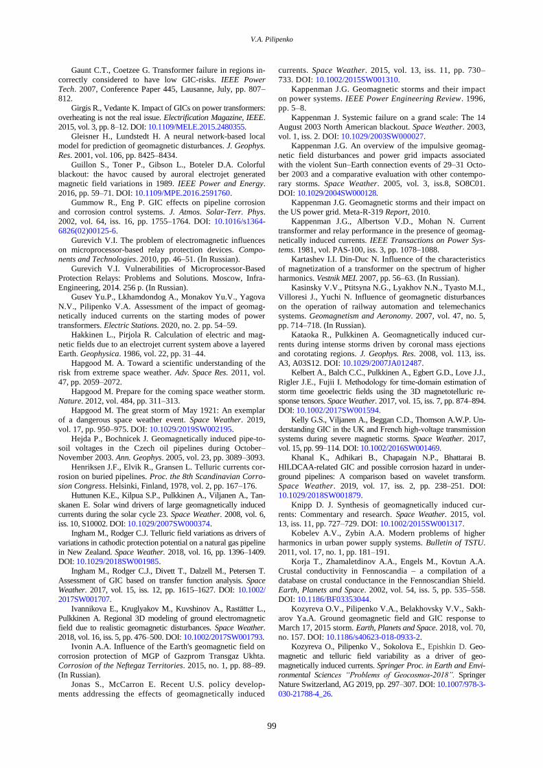
V.A. Pilipenko
99
Gaunt C.T., Coetzee G. Transformer failure in regions in-
correctly considered to have low GIC-risks. IEEE Power
Tech. 2007, Conference Paper 445, Lausanne, July, pp. 807–
812.
Girgis R., Vedante K. Impact of GICs on power transformers:
overheating is not the real issue. Electrification Magazine, IEEE.
2015, vol. 3, pp. 8–12. DOI: 10.1109/MELE.2015.2480355.
Gleisner H., Lundstedt H. A neural network-based local
model for prediction of geomagnetic disturbances. J. Geophys.
Res. 2001, vol. 106, pp. 8425–8434.
Guillon S., Toner P., Gibson L., Boteler D.A. Colorful
blackout: the havoc caused by auroral electrojet generated
magnetic field variations in 1989. IEEE Power and Energy.
2016, pp. 59–71. DOI: 10.1109/MPE.2016.2591760.
Gummow R., Eng P. GIC effects on pipeline corrosion
and corrosion control systems. J. Atmos. Solar-Terr. Phys.
2002, vol. 64, iss. 16, pp. 1755–1764. DOI: 10.1016/s1364-
6826(02)00125-6.
Gurevich V.I. The problem of electromagnetic influences
on microprocessor-based relay protection devices. Compo-
nents and Technologies. 2010, pp. 46–51. (In Russian).
Gurevich V.I. Vulnerabilities of Microprocessor-Based
Protection Relays: Problems and Solutions. Moscow, Infra-
Engineering, 2014. 256 p. (In Russian).
Gusev Yu.P., Lkhamdondog A., Monakov Yu.V., Yagova
N.V., Pilipenko V.A. Assessment of the impact of geomag-
netically induced currents on the starting modes of power
transformers. Electric Stations. 2020, no. 2. pp. 54–59.
Hakkinen L., Pirjola R. Calculation of electric and mag-
netic fields due to an electrojet current system above a layered
Earth. Geophysica. 1986, vol. 22, pp. 31–44.
Hapgood M. A. Toward a scientific understanding of the
risk from extreme space weather. Adv. Space Res. 2011, vol.
47, pp. 2059–2072.
Hapgood M. Prepare for the coming space weather storm.
Nature. 2012, vol. 484, pp. 311–313.
Hapgood M. The great storm of May 1921: An exemplar
of a dangerous space weather event. Space Weather. 2019,
vol. 17, pp. 950–975. DOI: 10.1029/2019SW002195.
Hejda P., Bochnicek J. Geomagnetically induced pipe-to-
soil voltages in the Czech oil pipelines during October–
November 2003. Ann. Geophys. 2005, vol. 23, pp. 3089–3093.
Henriksen J.F., Elvik R., Gransen L. Telluric currents cor-
rosion on buried pipelines. Proc. the 8th Scandinavian Corro-
sion Congress. Helsinki, Finland, 1978, vol. 2, pp. 167–176.
Huttunen K.E., Kilpua S.P., Pulkkinen A., Viljanen A., Tan-
skanen E. Solar wind drivers of large geomagnetically induced
currents during the solar cycle 23. Space Weather. 2008, vol. 6,
iss. 10, S10002. DOI: 10.1029/2007SW000374.
Ingham M., Rodger C.J. Telluric field variations as drivers of
variations in cathodic protection potential on a natural gas pipeline
in New Zealand. Space Weather. 2018, vol. 16, pp. 1396–1409.
DOI: 10.1029/2018SW001985.
Ingham M., Rodger C.J., Divett T., Dalzell M., Petersen T.
Assessment of GIC based on transfer function analysis. Space
Weather. 2017, vol. 15, iss. 12, pp. 1615–1627. DOI: 10.1002/
2017SW001707.
Ivannikova E., Kruglyakov M., Kuvshinov A., Rastätter L.,
Pulkkinen A. Regional 3D modeling of ground electromagnetic
field due to realistic geomagnetic disturbances. Space Weather.
2018, vol. 16, iss. 5, pp. 476–500. DOI: 10.1002/2017SW001793.
Ivonin A.A. Influence of the Earth's geomagnetic field on
corrosion protection of MGP of Gazprom Transgaz Ukhta.
Corrosion of the Neftegaz Territories. 2015, no. 1, pp. 88–89.
(In Russian).
Jonas S., McCarron E. Recent U.S. policy develop-
ments addressing the effects of geomagnetically induced
currents. Space Weather. 2015, vol. 13, iss. 11, pp. 730–
733. DOI: 10.1002/2015SW001310.
Kappenman J.G. Geomagnetic storms and their impact
on power systems. IEEE Power Engineering Review. 1996,
pp. 5–8.
Kappenman J. Systemic failure on a grand scale: The 14
August 2003 North American blackout. Space Weather. 2003,
vol. 1, iss. 2. DOI: 10.1029/2003SW000027.
Kappenman J.G. An overview of the impulsive geomag-
netic field disturbances and power grid impacts associated
with the violent Sun–Earth connection events of 29–31 Octo-
ber 2003 and a comparative evaluation with other contempo-
rary storms. Space Weather. 2005, vol. 3, iss.8, SO8C01.
DOI: 10.1029/2004SW000128.
Kappenman J.G. Geomagnetic storms and their impact on
the US power grid. Meta-R-319 Report, 2010.
Kappenman J.G., Albertson V.D., Mohan N. Current
transformer and relay performance in the presence of geomag-
netically induced currents. IEEE Transactions on Power Sys-
tems. 1981, vol. PAS-100, iss. 3, pp. 1078–1088.
Kartashev I.I. Din-Duc N. Influence of the characteristics
of magnetization of a transformer on the spectrum of higher
harmonics. Vestnik MEI. 2007, pp. 56–63. (In Russian).
Kasinsky V.V., Ptitsyna N.G., Lyakhov N.N., Tyasto M.I.,
Villoresi J., Yuchi N. Influence of geomagnetic disturbances
on the operation of railway automation and telemechanics
systems. Geomagnetism and Aeronomy. 2007, vol. 47, no. 5,
pp. 714–718. (In Russian).
Kataoka R., Pulkkinen A. Geomagnetically induced cur-
rents during intense storms driven by coronal mass ejections
and corotating regions. J. Geophys. Res. 2008, vol. 113, iss.
A3, A03S12. DOI: 10.1029/2007JA012487.
Kelbert A., Balch C.C., Pulkkinen A., Egbert G.D., Love J.J.,
Rigler J.E., Fujii I. Methodology for time‐domain estimation of
storm time geoelectric fields using the 3D magnetotelluric re-
sponse tensors. Space Weather. 2017, vol. 15, iss. 7, pp. 874–894.
DOI: 10.1002/2017SW001594.
Kelly G.S., Viljanen A., Beggan C.D., Thomson A.W.P. Un-
derstanding GIC in the UK and French high‐voltage transmission
systems during severe magnetic storms. Space Weather. 2017,
vol. 15, pp. 99–114. DOI: 10.1002/2016SW001469.
Khanal K., Adhikari B., Chapagain N.P., Bhattarai B.
HILDCAA-related GIC and possible corrosion hazard in under-
ground pipelines: A comparison based on wavelet transform.
Space Weather. 2019, vol. 17, iss. 2, pp. 238–251. DOI:
10.1029/2018SW001879.
Knipp D. J. Synthesis of geomagnetically induced cur-
rents: Commentary and research. Space Weather. 2015, vol.
13, iss. 11, pp. 727–729. DOI: 10.1002/2015SW001317.
Kobelev A.V., Zybin A.A. Modern problems of higher
harmonics in urban power supply systems. Bulletin of TSTU.
2011, vol. 17, no. 1, pp. 181–191.
Korja T., Zhamaletdinov A.A., Engels M., Kovtun A.A.
Crustal conductivity in Fennoscandia – a compilation of a
database on crustal conductance in the Fennoscandian Shield.
Earth, Planets and Space. 2002, vol. 54, iss. 5, pp. 535–558.
DOI: 10.1186/BF03353044.
Kozyreva O.V., Pilipenko V.A., Belakhovsky V.V., Sakh-
arov Ya.A. Ground geomagnetic field and GIC response to
March 17, 2015 storm. Earth, Planets and Space. 2018, vol. 70,
no. 157. DOI: 10.1186/s40623-018-0933-2.
Kozyreva O., Pilipenko V., Sokolova E., Epishkin D. Geo-
magnetic and telluric field variability as a driver of geo-
magnetically induced currents. Springer Proc. in Earth and Envi-
ronmental Sciences “Problems of Geocosmos-2018”. Springer
Nature Switzerland, AG 2019, pp. 297–307. DOI: 10.1007/978-3-
030-21788-4_26.
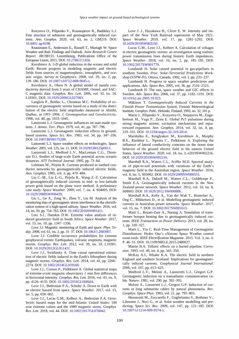
Space weather impact on ground-based technological systems
100
Kozyreva O., Pilipenko V., Krasnoperov R., Baddeley L.J.
Fine structure of substorm and geomagnetically induced cur-
rents. Ann. Geophys. 2020, vol. 63, no. 2, GM219. DOI:
10.4401/ ag-8198.
Krausmann E., Andersson E., Russell T., Murtagh W. Space
Weather and Rail: Findings and Outlook. Joint Research Centre
Report. JRC98155. Luxembourg, Publications Office of the
European Union, 2015. DOI: 10.2788/211456.
Kuvshinov A. 3-D global induction in the oceans and solid
Earth: Recent progress in modeling magnetic and electric
fields from sources of magnetospheric, ionospheric, and oce-
anic origin. Survey in Geophysics. 2008, vol. 29, iss. 2, pp.
139–186. DOI: 10.1007/s10712-008-9045-z.
Kuvshinov A., Olsen N. A global model of mantle con-
ductivity derived from 5 years of CHAMP, Orsted, and SAC-
C magnetic data. Geophys. Res. Lett. 2006, vol. 33, iss. 18.
L18301. DOI: 10.1029/2006GL027083.
Langlois P., Bolduc L., Chouteau M.C. Probability of oc-
currence of geomagnetic storms based on a study of the distri-
bution of the electric field amplitudes measured in Abitibi,
Québec, in 1993–1994. J. Geomagnetism and Geoelectricity.
1996, vol. 48, pp. 1033–1041.
Lanzerotti L.J. Geomagnetic influences on man-made sys-
tems. J. Atmos. Terr. Phys. 1979, vol. 41, pp. 787–796.
Lanzerotti L.J. Geomagnetic induction effects in ground-
based systems. Space Sci. Rev. 1983, vol. 34, pp. 347–356.
DOI: 10.1007/BF00175289.
Lanzerotti L.J. Space weather effects on technologies. Space
Weather. 2001, vol. 125, iss. 11. DOI: 10.1029/GM125p0011. Lanzerotti L.J., Medford L.V., MacLennan C.G., Thom-
son D.J. Studies of large-scale Earth potential across oceanic
distances. ATT Technical Journal. 1995, pp. 73–84.
Lehtinen M., Pirjola R. Currents produced in earthed con-
ductor networks by geomagnetically induced electric fields.
Ann. Geophys. 1985, vol. 3, pp. 479–484.
Liu C.-M., Liu L.-G., Pirjola R., Wang Z.-Z. Calculation
of geomagnetically induced currents in mid- to low-latitude
power grids based on the plane wave method: A preliminary
case study. Space Weather. 2009, vol. 7, iss. 4. S04005. DOI:
10.1029/2008SW000439.
Liu L., Ge X., Zong W., Zhou Y., Liu M. Analysis of the
monitoring data of geomagnetic storm interference in the electrifi-
cation system of a high-speed railway. Space Weather. 2016, vol.
14, iss. 10, pp. 754–763. DOI: 10.1002/2016SW001411.
Lotz S.I., Danskin D.W. Extreme value analysis of in-
duced geoelectric field in South Africa. Space Weather. 2017,
vol. 15, iss. 10, pp. 1347–1356.
Love J.J. Magnetic monitoring of Earth and space. Phys. To-
day. 2008, vol. 61, iss. 2, pp. 31–37. DOI: 10.1063/1.2883907.
Love J.J. Credible occurrence probabilities for extreme
geophysical events: Earthquakes, volcanic eruptions, magnetic
storms. Geophys. Res. Lett. 2012, vol. 39, iss. 10, L10301.
DOI: 10.1029/2012GL051431.
Love J.J., Swidinsky A. Time causal operational estima-
tion of electric fields induced in the Earth's lithosphere during
magnetic storms. Geophys. Res. Lett. 2014, vol. 41, pp. 2266–
2274. DOI: 10.1002/2014GL059568.
Love J.J., Cosson P., Pulkkinen A. Global statistical maps
of extreme-event magnetic observatory 1 min first differences
in horizontal intensity. Geophys. Res. Lett. 2016, vol. 43, iss. 9,
pp. 4126–4135. DOI: 10.1002/2016GL068664.
Love J.J., Bedrosian P.A., Schultz A. Down to Earth with
an electric hazard from space. Space Weather. 2017, vol. 15,
iss. 5, pp. 658–662.
Love J.J., Lucas G.M., Kelbert A., Bedrosian P.A. Geoe-
lectric hazard maps for the mid-Atlantic United States: 100
year extreme values and the 1989 magnetic storm. Geophys.
Res. Lett. 2018, vol. 44. DOI: 10.1002/2017GL076042.
Love J. J., Hayakawa H., Cliver E. W. Intensity and im-
pact of the New York Railroad superstorm of May 1921.
Space Weather. 2019, vol. 17, pp. 1281–1292. DOI:
10.1029/2019SW002250.
Lucas G.M., Love J.J., Kelbert A. Calculation of voltages
in electric geomagnetic storms: an investigation using realistic
power transmission lines during historic Earth impedances.
Space Weather. 2018, vol. 16, iss. 2, pp. 185–195. DOI:
10.1002/2017SW001779.
Lundstedt H. Solar caused potential in gas-pipelines in
southern Sweden. Proc. Solar-Terrestrial Predictions Work-
shop (STPW-IV), Ottava, Canada, 1992, vol. I, pp. 233–237.
Lundstedt H. Progress in space weather predictions and
applications. Adv. Space Res. 2005, vol. 36, pp. 2516–2523.
Lundstedt H. The sun, space weather and GIC effects in
Sweden. Adv. Space Res. 2006, vol. 37, pp. 1182–1191. DOI:
10.1016/j.asr.2005.10.023.
Mäkinen T. Geomagnetically Induced Currents in the
Finnish Power Transmission System. Finnish Meteorological
Institute, Geophys. Publ., Helsinki, Finland, 1993, no. 32, 101 p.
Marin J., Pilipenko V., Kozyreva O., Stepanova M., Enge-
bretson M., Vega P., Zesta E. Global Рс5 pulsations during
strong magnetic storms: excitation mechanisms and equa-
torward expansion. Ann. Geophys. 2014, vol. 32, iss. 4, pp.
319–331. DOI: 10.5194/angeo-32-319-2014.
Marshalko E., Kruglyakov M., Kuvshinov A., Murphy
B.S., Rastätter L., Ngwira C., Pulkkinen A. Exploring the
influence of lateral conductivity contrasts on the storm time
behavior of the ground electric field in the eastern United
States. Space Weather. 2020, vol. 18, iss. 3, e2019SW002216.
DOI: 10.1029/2019SW002216.
Marshall R.A., Waters C.L., Sciffer M.D. Spectral analy-
sis of pipe-to-soil potentials with variations of the Earth’s
magnetic field in the Australian region. Space Weather. 2010,
vol. 8, iss. 5, S05002. DOI: 10.1029/2009SW000553.
Marshall R.A., Dalzell M., Waters C.L., Goldthorpe P.,
Smith E.A. Geomagnetically induced currents in the New
Zealand power network. Space Weather. 2012, vol. 10, iss. 8,
S08003. DOI: 10.1029/2012 SW000806.
Marshall R.A., Kelly A., Van der Walt T., Honecker A.,
Ong C., Mikkelsen D., et al. Modelling geomagnetic induced
currents in Australian power networks. Space Weather. 2017,
vol. 15, iss. 7. DOI: 10.1002/2017SW001613.
Marti L., Rezaei-Zare A., Narang A. Simulation of trans-
former hotspot heating due to geomagnetically induced cur-
rents. IEEE Transaction on Power Delivery. 2013, vol. 28, iss.
1, pp. 320–327.
Marti L., Yiu C. Real-Time Management of Geomagnetic
Disturbances: Hydro One’s eXtreme Space Weather control
room tools. IEEE Electrification Magazine. 2015. Vol. 3, no. 4.
P. 46–51. DOI: 10.1109/MELE.2015.2480637.
Martin B.A. Telluric effects on a buried pipeline. Corro-
sion. 1993, vol. 49, iss. 4, pp. 343–350.
McKay A.J., Whaler K.A. The electric field in northern
England and southern Scotland: Implications for geomagneti-
cally induced currents. Geophysical Journal International.
2006, vol. 167, pp. 613–625.
Medford L.V., Meloni A., Lanzerotti L.J., Gregori G.P.
Geomagnetic induction on a transatlantic communication ca-
ble. Nature. 1981, vol. 290, pp. 392–393.
Meloni A., Lanzerotti L.J., Gregori G.P. Induction of cur-
rents in long submarine cables by natural phenomena. Rev.
Geophys. Space Phys. 1983, vol. 21, pp. 795–803.
Messerotti M., Zuccarello F., Guglielmino S., Bothmer V.,
Lilensten J., Noci G., et al. Solar weather modelling and pre-
dicting. Space Sci. Rev. 2009, vol. 147, pp. 121–185. DOI:
10.1007/s11214-009-9574-x.
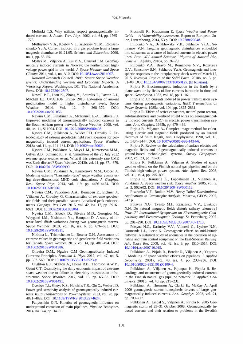
V.A. Pilipenko
101
Molinski T.S. Why utilities respect geomagnetically in-
duced currents. J. Atmos. Terr. Phys. 2002, vol. 64, pp. 1765–
1778.
Mullayarov V.A., Kozlov V.I., Grigoriev Yu.M., Romash-
chenko Yu.A. Current induced in a gas pipeline from a large
magnetic disturbance 01.21.05. Science and Education. 2006,
no. 1, pp. 53–55.
Myllys M., Viljanen A., Rui Ø.A., Ohnstad T.M. Geomag-
netically induced currents in Norway: the northernmost high-
voltage power grid in the world. J. Space Weather and Space
Climate. 2014, vol. 4, no. A10. DOI: 10.1051/swsc/2014007.
National Research Council. 2008. Severe Space Weather
Events: Understanding Societal and Economic Impacts: A
Workshop Report. Washington, DC: The National Academies
Press. DOI: 10.17226/12507.
Newell P.T., Liou K., Zhang Y., Sotirelis T., Paxton L.J.,
Mitchell E.J. OVATION Prime- 2013: Extension of auroral
precipitation model to higher disturbance levels, Space
Weather. 2014. Vol. 12, P. 368–379. DOI:
10.1002/2014sw001056.
Ngwira C.M., Pulkkinen A., McKinnell L.-A., Cilliers P.J.
Improved modeling of geomagnetically induced currents in
the South African power network. Space Weather. 2008, vol.
40, iss. 11, S11004. DOI: 10.1029/2008SW000408.
Ngwira C.M., Pulkkinen A., Wilder F.D., Crowley G. Ex-
tended study of extreme geoelectric field event scenarios for geo-
magnetically induced current applications. Space Weather.
2013a, vol. 11, pp. 121–131. DOI: 10.1002/swe.20021.
Ngwira C.M., Pulkkinen A., Mays L.M., Kuznetsova M.M.,
Galvin A.B., Simunac K., et al. Simulation of the 23 July 2012
extreme space weather event: What if this extremely rare CME
was Earth directed? Space Weather. 2013b, vol. 11, pp. 671–679.
DOI: 10.1002/2013SW000990.
Ngwira C.M., Pulkkinen A., Kuznetsova M.M., Glocer A.
Modeling extreme “Carrington-type” space weather events us-
ing three-dimensional MHD code simulations. J. Geophys.
Res.: Space Phys. 2014, vol. 119, pp. 4456–4474. DOI:
10.1002/2013JA019661.
Ngwira C.M., Pulkkinen A.A., Bernabeu E., Eichner J.,
Viljanen A., Crowley G. Characteristics of extreme geoelec-
tric fields and their possible causes: Localized peak enhance-
ments. Geophys. Res. Lett. 2015, vol. 42, iss. 17, pp. 6916–
6921. DOI: 10.1002/2015GL065061.
Ngwira C.M., Sibeck D., Silveira M.D., Georgiou M.,
Weygand J.M., Nishimura Yu., Hampton D. A study of in-
tense local dB/dt variations during two geomagnetic storms.
Space Weather. 2018, vol. 16, iss. 6, pp. 676–693. DOI:
10.1029/2018SW001911.
Nikitina L., Trichtchenko L., Boteler D.H. Assessment of
extreme values in geomagnetic and geoelectric field variations
for Canada. Space Weather. 2016, vol. 14, pp. 481–494. DOI:
10.1002/2016SW001386.
Oliveira D.M., Ngwira C.M Geomagnetically Induced
Currents: Principles. Brazilian J. Phys. 2017, vol. 47, no. 5,
pp. 552–560. DOI: 10.1007/s13538-017-0523-y. Oughton E.J., Skelton A., Horne R.B., Thomson A.W.P.,
Gaunt C.T. Quantifying the daily economic impact of extreme
space weather due to failure in electricity transmission infra-
structure. Space Weather. 2017, vol. 15, pp. 65–83. DOI:
10.1002/2016SW001491.
Overbye T.J., Shetye K.S., Hutchins T.R., Qiu Q., Weber J.D.
Power grid sensitivity analysis of geomagnetically induced cur-
rents. IEEE Transactions on Power Systems. 2013, vol. 28. pp.
4821–4828. DOI: 10.1109/TPWRS.2013.2274624.
Panyushkin G.N. Kinetics of geomagnetic influence on
underground corrosion of main pipelines. Pipeline Transport.
2014, no. 3-4, pp. 34–35.
Piccinelli R., Krausmann E. Space Weather and Power
Grids — A Vulnerability assessment. Report to European Un-
ion, Luxembourg, 2014, 53 p. DOI: 10.2788/20848.
Pilipenko V.А., Belakhovsky V.B., Sakharov Ya.A., Se-
livanov V.N. Irregular geomagnetic disturbances embedded
into substorms as a cause of induced currents in electric power
lines. Proc. XLI Annual Seminar “Physics of Auroral Phe-
nomena”. Apatity, 2018a, pp. 26–29.
Pilipenko V.A., Bravo M., Romanova N.V., Kozyreva
O.V., Samsonov S.N., Sakharov Ya.A. Geomagnetic and iono-
spheric responses to the interplanetary shock wave of March 17,
2015. Izvestiya. Physics of the Solid Earth. 2018b, no. 5, pp.
61–80. DOI: 10.1134/S0002333718050125. (In Russian).
Pirjola R. Electromagnetic induction in the Earth by a
plane wave or by fields of line currents harmonic in time and
space. Geophysica. 1982, vol. 18, pp. 1–161.
Pirjola R. On currents induced in power transmission sys-
tems during geomagnetic variations. IEEE Transactions on
Power Systems. 1985a, vol. 104, pp. 2825–2831.
Pirjola R. Effect of series capacitors, neutral point reactor,
autotransformers and overhead shield wires on geomagnetical-
ly induced currents (GIC) in electric power transmission sys-
tems. Ann. Geophys. 1985b, pp. 479–484. Pirjola R., Viljanen A., Complex image method for calcu-
lating electric and magnetic fields produced by an auroral electrojet of finite length, Ann. Geophysicae. 1998, vol. 16,
pp. 1434–1444. DOI: 10.1007/s00585-998-1434-6. Pirjola R. Review on the calculation of surface electric and
magnetic fields and of geomagnetically induced currents in ground-based technological systems. Survey Geophysics.
2002, vol. 23, pp. 71–90. Pirjola R., Pulkkinen A., Viljanen A. Studies of space
weather effects on the Finnish natural gas pipeline and on the Finnish high-voltage power system. Adv. Space Res. 2003,
vol. 31, iss. 4, pp. 795–805. Pirjola R., Kauristie K., Lappalainen H., Viljanen A.,
Pulkkinen A. Space weather risk. Space Weather. 2005, vol. 3, iss. 2, S02A02. DOI: 10.1029/ 2004SW000112.
Pisarenko V.F., Rodkin M.V. Heavy-Tailed Distributions: Applications to Catastrophe Analysis. Moscow, GEOS, 2007,
242 p.
Ptitsyna N.G., Tyasto M.I., Kassinskii V.V., Lyakhov N.N. Do natural magnetic fields disturb railway telemetry?
Proc. 7th International Symposium on Electromagnetic Com-patibility and Electromagnetic Ecology. St. Petersburg, 2007.
pp. 281–290. DOI: 10.1109/EMCECO.2007.4371713. Ptitsyna N.G., Kasinsky V.V., Villoresi G., Lyahov N.N.,
Dormande L.I., Iuccic N. Geomagnetic effects on mid-latitude
railways: A statistical study of anomalies in the operation of sig-naling and train control equipment on the East-Siberian Railway.
Adv. Space Res. 2008, vol. 42, iss. 9, pp. 1510–1514. DOI: 10.1016/j.asr.2007.10.015.
Pulkkinen A., Pirjola R., Boteler D., Viljanen A., Yegorov
I. Modeling of space weather effects on pipelines. J. Applied
Geophysics. 2001a, vol. 48, iss. 4, pp. 233–256. DOI: 10.1016/S0926-9851(01)00109-4.
Pulkkinen A., Viljanen A., Pajunpaa K., Pirjola R. Re-cordings and occurrence of geomagnetically induced currents
in the Finnish natural gas pipeline network. J. Applied Geo-physics. 2001b, vol. 48, pp. 219–231.
Pulkkinen A., Thomson A., Clarke E., McKay A. April
2000 geomagnetic storm: ionospheric drivers of large geo-magnetically induced currents. Ann. Geophys. 2003, vol. 21,
pp. 709–717. Pulkkinen A., Lindal S., Viljanen A., Pirjola R. 2005 Geo-
magnetic storm of 29–31 October 2003: Geomagnetically in-duced currents and their relation to problems in the Swedish
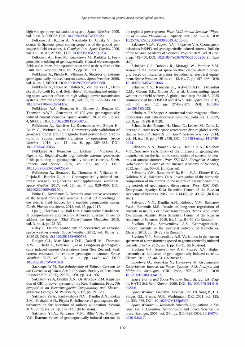
Space weather impact on ground-based technological systems
102
high-voltage power transmission system. Space Weather. 2005,
vol. 3, iss. 8, S08C03. DOI: 10.1029/2004SW000123.
Pulkkinen A., Klimas A., Vassiliadis D., Uritsky V., Tan-
skanen E. Spatiotemporal scaling properties of the ground geo-
magnetic field variations. J. Geophys. Res.: Space Physics. 2006,
vol. 111, iss. A3, A03305. DOI: 10.1029/2005JA011294.
Pulkkinen A., Hesse M., Kuznetsova M., Rastätter L. First-
principles modeling of geomagnetically induced electromagnetic
fields and currents from upstream solar wind to the surface of the
Earth. Ann. Geophys. 2007, vol. 25, pp. 881–893.
Pulkkinen A., Pirjola R., Viljanen A. Statistics of extreme
geomagnetically induced current events. Space Weather. 2008,
vol. 6, iss. 7, S07001. DOI: 10.1029/2008SW000388.
Pulkkinen A., Hesse M., Habib S., Van der Zel L., Dam-
sky B., Policelli F., et al. Solar shield: Forecasting and mitigat-
ing space weather effects on high-voltage power transmission
systems. Natural Hazards. 2010, vol. 53, pp. 333–345. DOI:
10.1007/s11069-009-9432-x.
Pulkkinen A.A., Bernabeu E., Eichner J., Beggan C.,
Thomson A.W.P. Generation of 100-year geomagnetically
induced current scenarios. Space Weather. 2012, vol. 10, iss.
4, S04003. DOI: 10.1029/2011SW000750.
Pulkkinen A., Rastätter L., Kuznetsova M., Singer H.,
Balch C., Weimer D., et al. Communitywide validation of
geospace model ground magnetic field perturbation predic-
tions to support model transition to operations. Space
Weather. 2013, vol. 11, iss. 6, pp. 369–385. DOI:
10.1002/swe.20056.
Pulkkinen A., Bernabeu E., Eichner J., Viljanen A.,
Ngwira C. Regional-scale high-latitude extreme geoelectric
fields pertaining to geomagnetically induced currents. Earth,
Planets and Space. 2015, vol. 67, no. 93. DOI:
10.1186/s40623-015-0255-6.
Pulkkinen A., Bernabeu E., Thomson A., Viljanen A.,
Pirjola R., Boteler D., et al. Geomagnetically induced cur-
rents: science, engineering and applications readiness.
Space Weather. 2017, vol. 15, iss. 7, pp. 828–856. DOI:
10.1002/2016SW001501.
Püthe C., Kuvshinov A. Towards quantitative assessment
of the hazard from space weather. Global 3D modellings of
the electric field induced by a realistic geomagnetic storm.
Earth, Planets and Space. 2013, vol. 65, pp. 1017.
Qiu Q., Fleeman J.A., Ball D.R. Geomagnetic disturbance.
A comprehensive approach by American Electric Power to
address the impacts. IEEE Electrification Magazine. 2015,
vol. 3, no. 4, pp. 22–33.
Riley P. On the probability of occurrence of extreme
space weather events. Space Weather. 2012, vol. 10, iss. 2,
S02012. DOI: 10.1029/2011SW000734.
Rodger C.J., Mac Manus D.H., Dalzell M., Thomson
A.W.P., Clarke E., Petersen T., et al. Long-term geomagneti-
cally induced current observations from New Zealand: Peak
current estimates for extreme geomagnetic storms. Space
Weather. 2017, vol. 15, iss. 11, pp. 1447–1460. DOI:
10.1002/2017SW001691.
Sackinger W.M. The Relationship of Telluric Currents to
the Corrosion of Warm Arctic Pipelines. Society of Petroleum
Engineer Publ. (SPE), 22099, 1991, pp. 361–366.
Sakharov Ya.A, Danilin A.N., Ostafiychuk R.M. Registra-
tion of GIC in power systems of the Kola Peninsula. Proc. 7th
Symposium on Electromagnetic Compatibility and Electro-
magnetic Ecology. St. Petersburg: 2007, pp. 291–293.
Sakharov Ya.A., Kudryashova N.V., Danilin A.N., Kokin
S.M., Shabalin A.N., Pirjola R. Influence of geomagnetic dis-
turbances on the operation of railway automation. Vestnik
MIIT. 2009, iss. 21, pp. 107–111. (In Russian).
Sakharov Ya.A., Selivanov V.N., Bilin V.A., Nikolaev
V.G. Extreme values of geomagnetically induced currents in
the regional power system. Proc. XLII Annual Seminar “Phys-
ics of Auroral Phenomena”. Apatity, 2019, pp. 53–56. DOI:
10.25702/KSC.2588-0039.2019.42.53-56.
Sakharov Ya.A., Yagova N.V., Pilipenko V.A. Geomagnetic
pulsations Pc5/Pi3 and geomagnetically induced currents. Bulletin
of the Russian Academy of Sciences: Physics. 2021, vol. 85, no.
3, pp. 445–450. DOI: 10.31857/s0367676521030236. (In Rus-
sian).
Schrijver C.J., Dobbins R., Murtagh W., Petrinec S.M.
Assessing the impact of space weather on the electric power
grid based on insurance claims for industrial electrical equip-
ment. Space Weather. 2014, vol. 12, iss. 7, pp. 487–498. DOI:
10.1002/2014SW001066.
Schrijver C.S., Kauristie K., Aylward A.D., Denardini
C.M., Gibson S.E., Glover A., et al. Understanding space
weather to shield society: A global road map for 2015–2025
commissioned by COSPAR and ILWS. Adv. Space Res. 2015,
vol. 55, no. 12, pp. 2745–2807. DOI: 10.1016/
j.asr.2015.03.023.
Schultz A. EMScope: A continental scale magneto-telluric
observatory and data discovery resource. Data Sci. J. 2009,
vol. 8, pp. IGY6–IGY20.
Schulte in den Baumen H., Moran D., Lenzen M., Cairns I.,
Steenge A. How severe space weather can disrupt global supply
chains? Natural Hazards and Earth System Sciences. 2014,
vol. 14, iss. 10, pp. 2749–2759. DOI: 10.5194/nhess-14-2749-
2014.
Selivanov V.N., Barannik M.B., Danilin A.N., Kolobov
V.V., Sakharov Ya.A. Study of the influence of geomagnetic
disturbances on the harmonic composition of currents in neu-
trals of autotransformers. Proc. KSC RAS: Energetika. Apatity:
Kola Scientific Center of the Russian Academy of Sciences,
2012, iss. 4, pp. 60–68. (In Russian).
Selivanov V.N., Barannik M.B., Bilin V.A., Efimov B.V.,
Kolobov V.V., Sakharov Ya.A. Investigation of the harmonic
composition of the current in the neutral of a transformer dur-
ing periods of geomagnetic disturbances. Proc. KSC RAS:
Energetika. Apatity: Kola Scientific Center of the Russian
Academy of Sciences. 2017, no. 1-14 (8), pp. 43–52. (In Rus-
sian).
Selivanov V.N., Danilin A.N., Kolobov V.V., Sakharov
Ya.A., Barannik M.B. Results of long-term registration of
currents in neutrals of power transformers. Trans. KSC RAS:
Energetika. Apatity: Kola Scientific Center of the Russian
Academy of Sciences, 2010. Iss. 1, pp. 84–90. (In Russian).
Sivokon V.P., Serovetnikov A.S. Geomagnetically-
induced currents in the electrical network of Kamchatka.
Electro. 2013, pp. 19–22. (In Russian).
Sivokon V.P., Serovetnikov A.S. Variations in the current
spectrum of a transformer exposed to geomagnetically induced
currents. Electro. 2015, no. 1, pp. 18–21. (In Russian).
Sivokon V.P., Serovetnikov A.S., Pisarev A.V. Higher
harmonics as indicators of geomagnetically induced currents.
Electro. 2011, pp. 44–51. (In Russian).
Sokolova O., Korovkin N., Hayakawa M. Geomagnetic
Disturbances Impacts on Power Systems: Risk Analysis and
Mitigation Strategies. CRC Press, 2021, 268 p. DOI:
10.1201/9781003134152.
Space Storms and Space Weather Hazards. Ed. I.A. Dag-
lis. NATO Sci. Ser., Kluwer, 2000. DOI: 10.1007/978-94-010-
0983-6.
Space Weather. Geophys. Monogr. Ser. Ed. Song P., H.J.
Singer, G.L. Siscoe, AGU, Washington, D.C. 2001. vol. 125.
pp. 353–358. DOI: 10.1029/GM125p0353.
Space Weather — Research Towards Applications in Eu-
rope. Ed. J. Lilensten. Astrophysics and Space Science Li-
brary, Springer. 2007, vol. 344, pp. 311–326. DOI: 10.1007/1-
4020-5446-7.
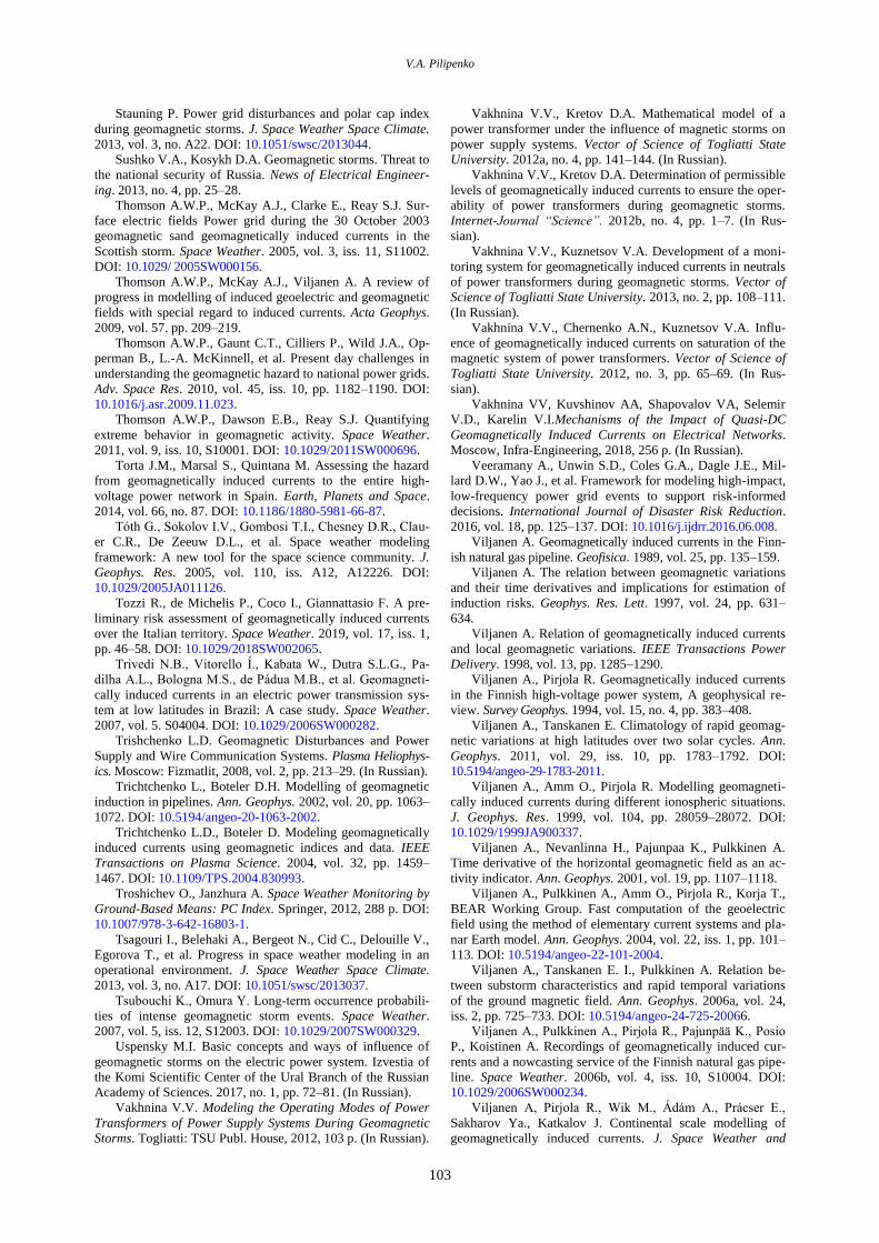
V.A. Pilipenko
103
Stauning P. Power grid disturbances and polar cap index
during geomagnetic storms. J. Space Weather Space Climate.
2013, vol. 3, no. A22. DOI: 10.1051/swsc/2013044.
Sushko V.A., Kosykh D.A. Geomagnetic storms. Threat to
the national security of Russia. News of Electrical Engineer-
ing. 2013, no. 4, pp. 25–28.
Thomson A.W.P., McKay A.J., Clarke E., Reay S.J. Sur-
face electric fields Power grid during the 30 October 2003
geomagnetic sand geomagnetically induced currents in the
Scottish storm. Space Weather. 2005, vol. 3, iss. 11, S11002.
DOI: 10.1029/ 2005SW000156.
Thomson A.W.P., McKay A.J., Viljanen A. A review of
progress in modelling of induced geoelectric and geomagnetic
fields with special regard to induced currents. Acta Geophys.
2009, vol. 57. pp. 209–219.
Thomson A.W.P., Gaunt C.T., Cilliers P., Wild J.A., Op-
perman B., L.-A. McKinnell, et al. Present day challenges in
understanding the geomagnetic hazard to national power grids.
Adv. Space Res. 2010, vol. 45, iss. 10, pp. 1182–1190. DOI:
10.1016/j.asr.2009.11.023.
Thomson A.W.P., Dawson E.B., Reay S.J. Quantifying
extreme behavior in geomagnetic activity. Space Weather.
2011, vol. 9, iss. 10, S10001. DOI: 10.1029/2011SW000696.
Torta J.M., Marsal S., Quintana M. Assessing the hazard
from geomagnetically induced currents to the entire high-
voltage power network in Spain. Earth, Planets and Space.
2014, vol. 66, no. 87. DOI: 10.1186/1880-5981-66-87.
Tóth G., Sokolov I.V., Gombosi T.I., Chesney D.R., Clau-
er C.R., De Zeeuw D.L., et al. Space weather modeling
framework: A new tool for the space science community. J.
Geophys. Res. 2005, vol. 110, iss. A12, A12226. DOI:
10.1029/2005JA011126.
Tozzi R., de Michelis P., Coco I., Giannattasio F. A pre-
liminary risk assessment of geomagnetically induced currents
over the Italian territory. Space Weather. 2019, vol. 17, iss. 1,
pp. 46–58. DOI: 10.1029/2018SW002065.
Trivedi N.B., Vitorello Í., Kabata W., Dutra S.L.G., Pa-
dilha A.L., Bologna M.S., de Pádua M.B., et al. Geomagneti-
cally induced currents in an electric power transmission sys-
tem at low latitudes in Brazil: A case study. Space Weather.
2007, vol. 5. S04004. DOI: 10.1029/2006SW000282.
Trishchenko L.D. Geomagnetic Disturbances and Power
Supply and Wire Communication Systems. Plasma Heliophys-
ics. Moscow: Fizmatlit, 2008, vol. 2, pp. 213–29. (In Russian).
Trichtchenko L., Boteler D.H. Modelling of geomagnetic
induction in pipelines. Ann. Geophys. 2002, vol. 20, pp. 1063–
1072. DOI: 10.5194/angeo-20-1063-2002.
Trichtchenko L.D., Boteler D. Modeling geomagnetically
induced currents using geomagnetic indices and data. IEEE
Transactions on Plasma Science. 2004, vol. 32, pp. 1459–
1467. DOI: 10.1109/TPS.2004.830993.
Troshichev O., Janzhura A. Space Weather Monitoring by
Ground-Based Means: PC Index. Springer, 2012, 288 p. DOI:
10.1007/978-3-642-16803-1.
Tsagouri I., Belehaki A., Bergeot N., Cid C., Delouille V.,
Egorova T., et al. Progress in space weather modeling in an
operational environment. J. Space Weather Space Climate.
2013, vol. 3, no. A17. DOI: 10.1051/swsc/2013037.
Tsubouchi K., Omura Y. Long‐term occurrence probabili-
ties of intense geomagnetic storm events. Space Weather.
2007, vol. 5, iss. 12, S12003. DOI: 10.1029/2007SW000329.
Uspensky M.I. Basic concepts and ways of influence of
geomagnetic storms on the electric power system. Izvestia of
the Komi Scientific Center of the Ural Branch of the Russian
Academy of Sciences. 2017, no. 1, pp. 72–81. (In Russian).
Vakhnina V.V. Modeling the Operating Modes of Power
Transformers of Power Supply Systems During Geomagnetic
Storms. Togliatti: TSU Publ. House, 2012, 103 p. (In Russian).
Vakhnina V.V., Kretov D.A. Mathematical model of a
power transformer under the influence of magnetic storms on
power supply systems. Vector of Science of Togliatti State
University. 2012a, no. 4, pp. 141–144. (In Russian).
Vakhnina V.V., Kretov D.A. Determination of permissible
levels of geomagnetically induced currents to ensure the oper-
ability of power transformers during geomagnetic storms.
Internet-Journal “Science”. 2012b, no. 4, pp. 1–7. (In Rus-
sian).
Vakhnina V.V., Kuznetsov V.A. Development of a moni-
toring system for geomagnetically induced currents in neutrals
of power transformers during geomagnetic storms. Vector of
Science of Togliatti State University. 2013, no. 2, pp. 108–111.
(In Russian).
Vakhnina V.V., Chernenko A.N., Kuznetsov V.A. Influ-
ence of geomagnetically induced currents on saturation of the
magnetic system of power transformers. Vector of Science of
Togliatti State University. 2012, no. 3, pp. 65–69. (In Rus-
sian).
Vakhnina VV, Kuvshinov AA, Shapovalov VA, Selemir
V.D., Karelin V.I.Mechanisms of the Impact of Quasi-DC
Geomagnetically Induced Currents on Electrical Networks.
Moscow, Infra-Engineering, 2018, 256 p. (In Russian).
Veeramany A., Unwin S.D., Coles G.A., Dagle J.E., Mil-
lard D.W., Yao J., et al. Framework for modeling high-impact,
low-frequency power grid events to support risk-informed
decisions. International Journal of Disaster Risk Reduction.
2016, vol. 18, pp. 125–137. DOI: 10.1016/j.ijdrr.2016.06.008.
Viljanen A. Geomagnetically induced currents in the Finn-
ish natural gas pipeline. Geofisica. 1989, vol. 25, pp. 135–159.
Viljanen A. The relation between geomagnetic variations
and their time derivatives and implications for estimation of
induction risks. Geophys. Res. Lett. 1997, vol. 24, pp. 631–
634.
Viljanen A. Relation of geomagnetically induced currents
and local geomagnetic variations. IEEE Transactions Power
Delivery. 1998, vol. 13, pp. 1285–1290.
Viljanen A., Pirjola R. Geomagnetically induced currents
in the Finnish high-voltage power system, A geophysical re-
view. Survey Geophys. 1994, vol. 15, no. 4, pp. 383–408.
Viljanen A., Tanskanen E. Climatology of rapid geomag-
netic variations at high latitudes over two solar cycles. Ann.
Geophys. 2011, vol. 29, iss. 10, pp. 1783–1792. DOI:
10.5194/angeo-29-1783-2011.
Viljanen A., Amm O., Pirjola R. Modelling geomagneti-
cally induced currents during different ionospheric situations.
J. Geophys. Res. 1999, vol. 104, pp. 28059–28072. DOI:
10.1029/1999JA900337.
Viljanen A., Nevanlinna H., Pajunpaa K., Pulkkinen A.
Time derivative of the horizontal geomagnetic field as an ac-
tivity indicator. Ann. Geophys. 2001, vol. 19, pp. 1107–1118.
Viljanen A., Pulkkinen A., Amm O., Pirjola R., Korja T.,
BEAR Working Group. Fast computation of the geoelectric
field using the method of elementary current systems and pla-
nar Earth model. Ann. Geophys. 2004, vol. 22, iss. 1, pp. 101–
113. DOI: 10.5194/angeo-22-101-2004.
Viljanen A., Tanskanen E. I., Pulkkinen A. Relation be-
tween substorm characteristics and rapid temporal variations
of the ground magnetic field. Ann. Geophys. 2006a, vol. 24,
iss. 2, pp. 725–733. DOI: 10.5194/angeo-24-725-20066.
Viljanen A., Pulkkinen A., Pirjola R., Pajunpää K., Posio
P., Koistinen A. Recordings of geomagnetically induced cur-
rents and a nowcasting service of the Finnish natural gas pipe-
line. Space Weather. 2006b, vol. 4, iss. 10, S10004. DOI:
10.1029/2006SW000234.
Viljanen A, Pirjola R., Wik M., Ádám A., Prácser E.,
Sakharov Ya., Katkalov J. Continental scale modelling of
geomagnetically induced currents. J. Space Weather and
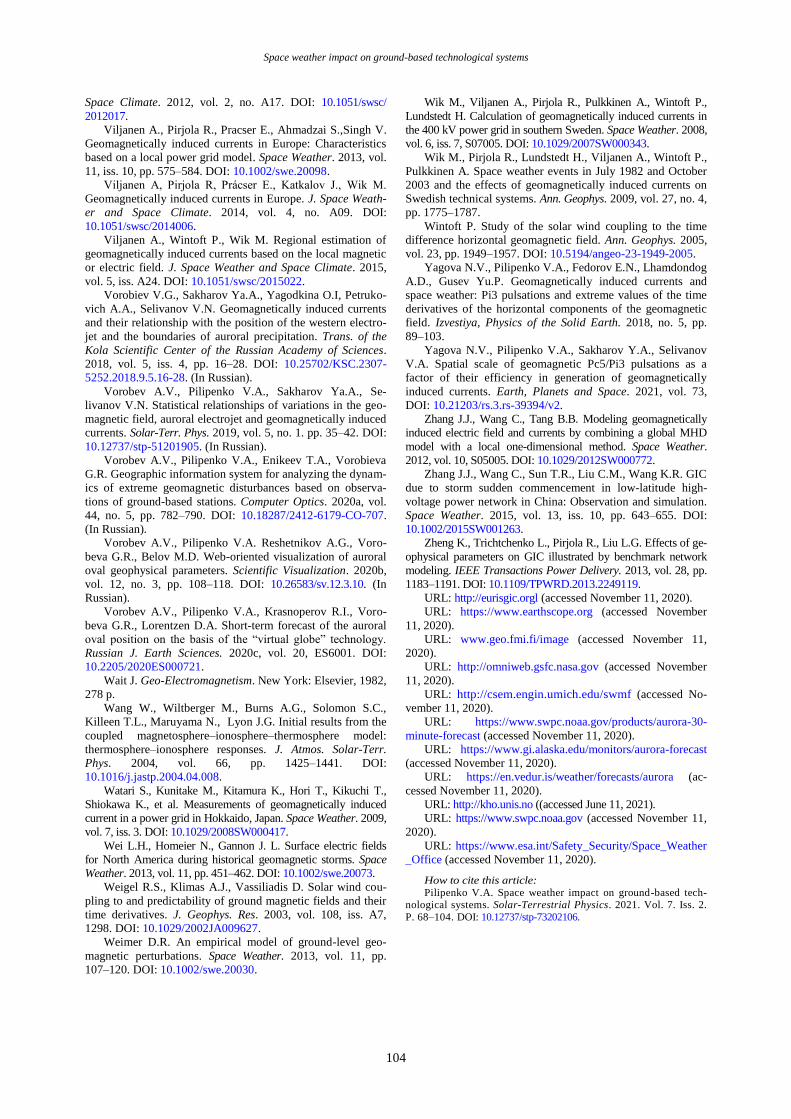
Space weather impact on ground-based technological systems
104
Space Climate. 2012, vol. 2, no. A17. DOI: 10.1051/swsc/
2012017.
Viljanen A., Pirjola R., Pracser E., Ahmadzai S.,Singh V.
Geomagnetically induced currents in Europe: Characteristics
based on a local power grid model. Space Weather. 2013, vol.
11, iss. 10, pp. 575–584. DOI: 10.1002/swe.20098.
Viljanen A, Pirjola R, Prácser E., Katkalov J., Wik M.
Geomagnetically induced currents in Europe. J. Space Weath-
er and Space Climate. 2014, vol. 4, no. A09. DOI:
10.1051/swsc/2014006.
Viljanen A., Wintoft P., Wik M. Regional estimation of
geomagnetically induced currents based on the local magnetic
or electric field. J. Space Weather and Space Climate. 2015,
vol. 5, iss. A24. DOI: 10.1051/swsc/2015022.
Vorobiev V.G., Sakharov Ya.A., Yagodkina O.I, Petruko-
vich A.A., Selivanov V.N. Geomagnetically induced currents
and their relationship with the position of the western electro-
jet and the boundaries of auroral precipitation. Trans. of the
Kola Scientific Center of the Russian Academy of Sciences.
2018, vol. 5, iss. 4, pp. 16–28. DOI: 10.25702/KSC.2307-
5252.2018.9.5.16-28. (In Russian).
Vorobev A.V., Pilipenko V.A., Sakharov Ya.A., Se-
livanov V.N. Statistical relationships of variations in the geo-
magnetic field, auroral electrojet and geomagnetically induced
currents. Solar-Terr. Phys. 2019, vol. 5, no. 1. pp. 35–42. DOI:
10.12737/stp-51201905. (In Russian).
Vorobev A.V., Pilipenko V.A., Enikeev T.A., Vorobieva
G.R. Geographic information system for analyzing the dynam-
ics of extreme geomagnetic disturbances based on observa-
tions of ground-based stations. Computer Optics. 2020a, vol.
44, no. 5, pp. 782–790. DOI: 10.18287/2412-6179-CO-707.
(In Russian).
Vorobev A.V., Pilipenko V.A. Reshetnikov A.G., Voro-
beva G.R., Belov M.D. Web-oriented visualization of auroral
oval geophysical parameters. Scientific Visualization. 2020b,
vol. 12, no. 3, pp. 108–118. DOI: 10.26583/sv.12.3.10. (In
Russian).
Vorobev A.V., Pilipenko V.A., Krasnoperov R.I., Voro-
beva G.R., Lorentzen D.A. Short-term forecast of the auroral
oval position on the basis of the “virtual globe” technology.
Russian J. Earth Sciences. 2020c, vol. 20, ES6001. DOI:
10.2205/2020ES000721.
Wait J. Geo-Electromagnetism. New York: Elsevier, 1982,
278 p.
Wang W., Wiltberger M., Burns A.G., Solomon S.C.,
Killeen T.L., Maruyama N., Lyon J.G. Initial results from the
coupled magnetosphere–ionosphere–thermosphere model:
thermosphere–ionosphere responses. J. Atmos. Solar-Terr.
Phys. 2004, vol. 66, pp. 1425–1441. DOI:
10.1016/j.jastp.2004.04.008.
Watari S., Kunitake M., Kitamura K., Hori T., Kikuchi T.,
Shiokawa K., et al. Measurements of geomagnetically induced
current in a power grid in Hokkaido, Japan. Space Weather. 2009,
vol. 7, iss. 3. DOI: 10.1029/2008SW000417.
Wei L.H., Homeier N., Gannon J. L. Surface electric fields
for North America during historical geomagnetic storms. Space
Weather. 2013, vol. 11, pp. 451–462. DOI: 10.1002/swe.20073.
Weigel R.S., Klimas A.J., Vassiliadis D. Solar wind cou-
pling to and predictability of ground magnetic fields and their
time derivatives. J. Geophys. Res. 2003, vol. 108, iss. A7,
1298. DOI: 10.1029/2002JA009627.
Weimer D.R. An empirical model of ground-level geo-
magnetic perturbations. Space Weather. 2013, vol. 11, pp.
107–120. DOI: 10.1002/swe.20030.
Wik M., Viljanen A., Pirjola R., Pulkkinen A., Wintoft P.,
Lundstedt H. Calculation of geomagnetically induced currents in
the 400 kV power grid in southern Sweden. Space Weather. 2008,
vol. 6, iss. 7, S07005. DOI: 10.1029/2007SW000343.
Wik M., Pirjola R., Lundstedt H., Viljanen A., Wintoft P.,
Pulkkinen A. Space weather events in July 1982 and October
2003 and the effects of geomagnetically induced currents on
Swedish technical systems. Ann. Geophys. 2009, vol. 27, no. 4,
pp. 1775–1787.
Wintoft P. Study of the solar wind coupling to the time
difference horizontal geomagnetic field. Ann. Geophys. 2005,
vol. 23, pp. 1949–1957. DOI: 10.5194/angeo-23-1949-2005.
Yagova N.V., Pilipenko V.A., Fedorov E.N., Lhamdondog
A.D., Gusev Yu.P. Geomagnetically induced currents and
space weather: Pi3 pulsations and extreme values of the time
derivatives of the horizontal components of the geomagnetic
field. Izvestiya, Physics of the Solid Earth. 2018, no. 5, pp.
89–103.
Yagova N.V., Pilipenko V.A., Sakharov Y.A., Selivanov
V.A. Spatial scale of geomagnetic Pc5/Pi3 pulsations as a
factor of their efficiency in generation of geomagnetically
induced currents. Earth, Planets and Space. 2021, vol. 73,
DOI: 10.21203/rs.3.rs-39394/v2.
Zhang J.J., Wang C., Tang B.B. Modeling geomagnetically
induced electric field and currents by combining a global MHD
model with a local one-dimensional method. Space Weather.
2012, vol. 10, S05005. DOI: 10.1029/2012SW000772.
Zhang J.J., Wang C., Sun T.R., Liu C.M., Wang K.R. GIC
due to storm sudden commencement in low-latitude high-
voltage power network in China: Observation and simulation.
Space Weather. 2015, vol. 13, iss. 10, pp. 643–655. DOI:
10.1002/2015SW001263.
Zheng K., Trichtchenko L., Pirjola R., Liu L.G. Effects of ge-
ophysical parameters on GIC illustrated by benchmark network
modeling. IEEE Transactions Power Delivery. 2013, vol. 28, pp.
1183–1191. DOI: 10.1109/TPWRD.2013.2249119.
URL: http://eurisgic.orgl (accessed November 11, 2020).
URL: https://www.earthscope.org (accessed November
11, 2020).
URL: www.geo.fmi.fi/image (accessed November 11,
2020).
URL: http://omniweb.gsfc.nasa.gov (accessed November
11, 2020).
URL: http://csem.engin.umich.edu/swmf (accessed No-
vember 11, 2020).
URL: https://www.swpc.noaa.gov/products/aurora-30-
minute-forecast (accessed November 11, 2020).
URL: https://www.gi.alaska.edu/monitors/aurora-forecast
(accessed November 11, 2020).
URL: https://en.vedur.is/weather/forecasts/aurora (ac-
cessed November 11, 2020).
URL: http://kho.unis.no ((accessed June 11, 2021).
URL: https://www.swpc.noaa.gov (accessed November 11,
2020).
URL: https://www.esa.int/Safety_Security/Space_Weather
_Office (accessed November 11, 2020).
How to cite this article:
Pilipenko V.A. Space weather impact on ground-based tech-nological systems. Solar-Terrestrial Physics. 2021. Vol. 7. Iss. 2.
P. 68–104. DOI: 10.12737/stp-73202106.