1077-2626/13/$31.00 © 2013 IEEE Published by the IEEE Computer Society

Accepted for publication by IEEE. ©2013 IEEE. Personal use of this material is permitted. Permission from IEEE must be obtained for all other uses, in any current or future media, including reprinting/republishing this material for advertising or promotional purposes, creating new collective works, for resale or redistribution to servers or lists, or reuse of any copyrighted component of this work in other works.

Space Transformation for Understanding Group Movement

Natalia Andrienko, Gennady Andrienko, Louise Barrett, Marcus Dostie, and Peter Henzi

Abstract—We suggest a methodology for analyzing movement behaviors of individuals moving in a group. Group movement is analyzed at two levels of granularity: the group as a whole and the individuals it comprises. For analyzing the relative positions and movements of the individuals with respect to the rest of the group, we apply space transformation, in which the trajectories of the individuals are converted from geographical space to an abstract “group space”. The group space reference system is defined by both the position of the group center, which is taken as the coordinate origin, and the direction of the group's movement. Based on the individuals’ positions mapped onto the group space, we can compare the behaviors of different individuals, determine their roles and/or ranks within the groups, and, possibly, understand how group movement is organized. The utility of the methodology has been evaluated by applying it to a set of real data concerning movements of wild social animals and discussing the results with experts in animal ethology.

Index Terms—Visual analytics, movement data, collective movement

INTRODUCTION

While movement data (trajectories of moving objects) have been in the research focus in the fields of database science [1][2], spatial computing [3][4], machine learning and data mining [5][6], and visual analytics [7][8][9] over the recent years, quite little has been done so far for supporting the analysis of group movement, i.e., for helping analysts to find answers to specific types of questions concerning the movement behavior of a group as a whole and of its members in relation to each other. Such questions arise, in particular, in the research of behaviors of various collective animals. The term ‘group movement’ denotes a specific kind of movement behavior when multiple related objects move together driven by a common purpose or common reason. It does not apply to simultaneous movements of multiple independent objects, e.g., to vehicle traffic.

We propose a novel approach to analyzing group movement that is based on computing the central trajectory of a group and transforming the coordinates of the group members to relative positions with respect to the group center and movement direction. The set of all possible relative positions is regarded as the ‘group space’. After the mapping onto the group space, the data can be visualized and analyzed using various existing methods. The transformation allows the analysts to abstract from the changes of the position of the group in the original (geographic) space and focus on the relative positions of the objects in the group and their changes over time. This paper presents the algorithm for the central trajectory computation and space transformation and shows how its results can be exploited in data analysis using two data examples: a small dataset, for which detailed analysis can be done, and a larger dataset, which is analyzed using scalable methods involving data aggregation and clustering.

1 RELATED WORKS

The research dealing with collective movement can be classified into four categories: theories and conceptual models, collective pattern identification in movement data, study of movement of a given collective, and collective movement simulation. Here we omit the fourth category as not really relevant to our work.

1.1 Theories and Conceptual Models

There are many publications in which various types of collective movement patterns are defined. Based on a literature survey, Dodge et al. [10] organize the existing definitions of movement patterns, including collective ones, in a taxonomy, and Laube [3] surveys the state of the art in movement pattern analysis, including pattern definitions. An example of collective movement pattern is ‘flock’, which is very popular in data mining literature and even considered as the quintessential movement pattern [3]: a flock in a time interval I=[ti,tj], where j-i+1≤ k, consists of at least m entities such that for every time instant within I there is a disk of radius r that contains all the m entities [11]. Here, k, m, and r are parameters. In a similar way, other types of patterns are defined. Thus, in a ‘herd’ [12], the entities in each time instant must form a dense spatial cluster, and so on.

In a series of papers [13][14][15] and a Ph.D. thesis [16], Wood and Galton develop a general taxonomy of collectives and a more specific taxonomy of spatial collectives. Three forms of spatial coherence define a spatial collective: common location, which may be fixed or variable, similar movement parameters (speed and direction), and formation, i.e., the positions of the individuals in relation to each other. If the individuals always maintain their relative positions, the formation is constant, if they only intermittently maintain their relative positions, the formation is called canonical, and if the individuals never maintain their relative positions, they have no formation. At least one form of spatial coherence is necessary for considering a set of individuals as a spatial collective. The characteristics used to classify spatial collectives include membership (constant or variable), correlation between the motions of the whole collective and its individuals (correlated or uncorrelated), depth (whether none, some, or all collective members are themselves collectives), and a few others.

Compared to the general taxonomy of collectives, the taxonomy of spatial collectives does not include the characteristics in terms of the role structure and the intercommunications and interactions between the individuals because relevant information is typically not available in movement data. Although it may be possible to identify a single leader [10][17], it is unlikely that a leading group can be singled out, and other roles can hardly be differentiated. Interactions between individuals, such as collision avoidance, velocity matching, flock centering [18], attraction, repulsion, and alignment [19] are modeled in simulations of collective movements but cannot be derived from data reflecting real movements.

Wood and Galton [13]-[16] suggest a framework called TLA (Three Level Analysis) in which collective movement is examined at three levels of spatial granularity: the motion of the whole collective considered as a unit, the evolution of the collective’s footprint, and the motions exhibited by the individual members.

• Natalia Andrienko and Gennady Andrienko are with Fraunhofer

Institute IAIS. E-mail: {natalia|gennady}.andrienko@iais.fraunhofer.de.• Louise Barrett, Marcus Dostie,and Peter Henzi are with University of

Lethbridge and University of South Africa. E-mail: {louise.barrett, marcus.dostie, peter.henzi}@uleth.ca.

Manuscript received 31 March 2013; accepted 1 August 2013; posted online13 October 2013; mailed on 4 October 2013. For information on obtaining reprints of this article, please send e-mail to: tvcg@computer.org.

1.2 Detection of Collective Movement Patterns

Wood [16] incorporates her theoretical model in research software that analyzes movement data to find groups of individuals exhibiting some form of spatial coherence.

In data mining and spatial computing, numerous algorithms have been developed for finding specific types of collective movement patterns in movement data [20]: ‘flock’, ‘leadership’, ‘convergence’, ‘encounter’ [21][22], ‘trend setting’ (movements of some individual are repeated by others after a time lag) [17], ‘moving cluster’ [23], ‘herd’ [12], etc.; Laube [3] and Gudmundsson et al. [24] present reviews of the existing methods.

1.3 Analysis of Collective Movement

Some of the pattern detection methods can be used for finding “leaders” and “trend setters” within a given collective of moving objects [17][21][22][25]. A “leader” is an object that moves in front of the others and a “trend setter” is an object whose movements are copied by the others.

For animal collectives [26], it is known that leaders do not necessarily move in front of a group. Therefore, Nagy et al. [27] use a definition of “leading” that is close to “trend setting” [17]: a leading event occurs when one object’s movement direction is copied by another object delayed in time. From trajectories of pigeons flying in a flock, Nagy et al. compute for each pair of birds the correlations between their movement directions for different time lags and select the time lag for which the correlation is maximal. On this basis, they compose a leader-follower network, where the nodes represent the birds and directed links represent the leader-follower relations. Two nodes are connected by a link if the maximal directional correlation between the respective birds exceeds a chosen threshold. This method was applied to data from multiple flights. For most of them, robust hierarchical networks could be constructed. Nagy et al. identified the individuals that contributed more than others to the movement decisions of the flock through having followers who consistently copied their movements. The leaders tended to occupy positions near the front of the flock. Interestingly, a tendency of the pigeons to follow partners that fly to their left, i.e., perceived by the left eye, has been discovered. This suggests that social information may be preferentially processed through the left-eye/right-hemispheric system. It should be noted that the reported study was possible owing to the high temporal resolution of the data (0.2 seconds).

In visual analytics, many methods for analysis of movement data have been developed recently [7]. Although these methods are applicable to data concerning collective movements, they do not address questions specific to analyzing collective movements, such as: What is the course of the whole group? How compact or dispersed is the group in space and how does this change over space and time? How coherent are the movements of the group members? Which individuals tend to lead and which tend to follow? Are these tendencies stable or change over time? We have found only one visual analytics paper [28] specifically addressing group movement. The authors compute attributes characterizing the positions and movements of each member in relation to the group: the distances to the group midpoint and boundary, the differences of the individual speeds and directions to the speed and direction of the group, and whether an object is in the group core or is an outlier, based on the definition of outlierness given by Wilkinson et al. [29]. The derived attributes are visualized on time graphs (temporal line charts), which are used for attribute-based filtering. The trajectory segments satisfying the filter are shown on a map display. To compare movements in two or more groups, the lines on the time graphs can be colored according to group membership.

2 OUR CONTRIBUTION

We present a novel approach to group movement analysis, which can complement the existing methods by providing a new perspective for looking at group movement. The key idea of the approach is space

transformation: the coordinates of the group members in the physical (geographical) space are transformed into relative positions with respect to the group center and movement direction. This replaces the physical space by an abstract group space. The positions and movements of the group members within the group space can be investigated regardless of the whereabouts of the group in the physical space.

2.1 An Example of Space Transformation

To illustrate the idea, we use a dataset with trajectories of 12 people who took part in a group walk, during which they tracked their movements by means of GPS devices. The group members agreed to provide the collected data for research purposes.

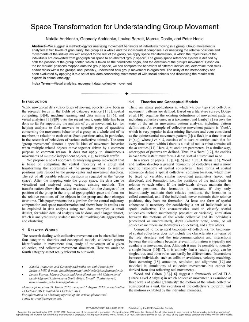
In Fig.1, the trajectories of the walkers in the geographic space are shown on a map (A) and in a space-time cube (B) [30][31], where the base represents the geographical space and the vertical dimension represents the time. The time axis is oriented upwards. Figure 2 shows the same trajectories transformed to the space where the coordinate system is defined by the group center (the origin of the coordinates) and the group movement direction (the Y-axis). On the left, the group space with the transformed trajectories is shown on a map. The map contains X- and Y-axes; their crossing marks the group center. The front part of the group is above the X-axis and the

Fig. 1. Original trajectories of multiple individuals that walked in a group are visualized on a map (A) and in a space-time cube (B).

Fig. 2. The trajectories of the group members have been transformed from the geographic space to an abstract group space where the coordinate system origin is the group center and the Y-axis reflects the direction of the group movement. The transformed trajectories are shown on a map (A) and in a space-time cube (B).

Fig.3. After converting the trajectories to the group space, subsets of trajectories can be selected for visual inspection and comparison.

rear part is below the X-axis. On the right, the transformed trajectories are shown in a space-time cube. The cube is turned so that the Y-axis goes from left to right; hence, the front part of the group is on the right and the rear part is on the left of the cube view.

Using the transformed trajectories, the movement behaviors of the individuals within the group can be investigated and compared. To reduce the display clutter, one or a few trajectories are selected for detailed visual inspection, as in Fig.3. For example, we can observe on the left that the person whose trajectory is colored in dark blue was in the front part of the group almost all the time but at the end moved to the back. The cyan-colored trajectory line shows that the respective person was initially at the group center, then moved to the back, but by the end of the trip moved to the front. The brown trajectory line has a long part almost coinciding with a part of the cyan line, which may mean that the respective individuals walked together during a long time interval. On the right of Fig.3, we can compare the trajectories of three persons who tended to take the front positions in the group. The green trajectory was behind the two others in the first half of the walk but then moved to the front and mostly preserved this position. The dark blue trajectory was more frequently in front of the others in the first half of the walk. There was a time interval when all three “leaders” were close together, then they separated. Such observations would be hardly possible with the use of the original trajectories (Fig.1).

2.2 The Space Transformation Method

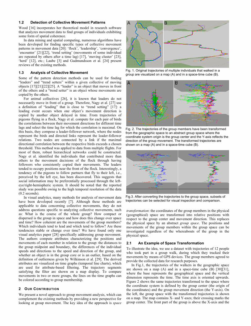
The method allowing us to map the positions of group members from the geographical space onto a group space is based on constructing the central trajectory of the group. The central trajectory represents the route followed by the group as a whole. The central trajectory for our example group of walkers is shown in Fig.4. The following algorithm describes the construction of the central

trajectory and the computation of variables necessary for the space transformation.

Algorithm 1: Construction of the central trajectory of a group Given:

- Set of trajectories Tr = {tr1, tr2, ..., trN} of moving objects O = {o1, o2, ..., oN}.

- Minimal distance threshold dmin: distances below dmin are treated as zero distances.

Description of the algorithm:

1. Extract all time references from the trajectories in Tr and create a chronologically ordered list of time units T = {t1, t2, ..., tM} without duplicates.

2. Create an empty trajectory CT. // central trajectory of the group 3. For each time unit ti ∈ T, do the following:

3.1. Create an empty set of points Pi. 3.2. // find the object positions at time ti:

For each oj ∈ O, find or estimate by interpolation the object position pij. If pij ≠ null, add pij to Pi. // pij may be null if the trajectory trj starts after or ends before ti.

3.3. // create a point representing the group center at time ti: Create a new point cpi = (x′, y′), where x′ and y′ are the mean x- and y-coordinates of the points in Pi. Attach (ti, cpi) to the trajectory CT.

4. For each time unit ti ∈ {t1, t2, ..., tM-1}, do the following: 4.1. // reconstruct the group movement vector:

Find such k (k = i+1, i+2, ..., M) that spatial_distance (cpi, cpk) ≥ dmin, where cpi and cpk are the points of CT corresponding to time units ti and tk. If k is not found, go to 5. // The points cpi and cpk define the group movement vector.

4.2. For each point pij (position of object oj at time tj), do the following: 4.2.1. Find the projection onto the group movement vector (cpi, cpk):

prij= projection_point(pij, (cpi, cpk)). 4.2.2. Let dx = spatial_distance (pij, prij). Let signed distance sdx = -dx if pij is

to the left of the movement vector (cpi, cpk) and sdx = dx otherwise. Attach sdx to pij as the X-coordinate in the group space.

4.2.3. Let sdy = spatial_distance (prij, cpi) ⋅ relative_position (prij, (cpi, cpk)), where relative_position (prij, (cpi, cpk)) equals 1 if prij is in front of cpi with respect to the direction of the vector (cpi, cpk) and -1 otherwise. Attach sdy to pij as the Y-coordinate in the group space.

5. Return CT and Tr. // The points of the trajectories in Tr has been enriched with the new variables specifying the positions of these points in the group space.

function projection_point (Point p, Vector (q1, q2)): 1. let dxq = q2.x – q1.x; let dyq = q2.y – q1.y; 2. if dxq = 0 and dyq = 0 then return null; // vector (q1, q2) has zero length 3. let dxp = p.x – q1.x; let dyp = p.y – q1.y; 4. let dot = dxp ⋅ dxq + dyp ⋅ dyq // dot product of the vectors (q1, p) and (q1, q2) 5. let u = dot / (dxq⋅ dxq + dyq⋅ dyq) 6. let x = q1.x + u ⋅ dxq; let y = q1.y + u ⋅ dyq; 7. return new Point(x, y);

function relative_position (Point p, Vector (q1, q2)): 1. let dxq = q2.x – q1.x; let dyq = q2.y – q1.y; 2. if dxq = 0 and dyq = 0 then return 0; // vector (q1, q2) has zero length 3. let dxp = p.x – q1.x; let dyp = p.y – q1.y; 4. let dot = dxp ⋅ dxq + dyp ⋅ dyq // dot product of the vectors (q1, p) and (q1, q2) 5. let u = dot / (dxq⋅ dxq + dyq⋅ dyq) 6. if u > 1 then return 1; else return -1;

Statements 4.2.1-4.2.3 describe how the positions of the original trajectory points in the group space are determined. Each original point is projected onto the movement vector of the group at the time moment of this point, as shown in Fig.5. The distance to the group movement vector, i.e., to the projection point, gives the x-coordinate in the group space. The x-coordinate is negative if the original point is to the left of the group movement vector and positive otherwise. The distance of the projection point to the group center, i.e., to the point of the central trajectory, gives the y-coordinate in the group space. The y-coordinate is positive if the projection point is in front of the group center and negative if it is behind the group center.

Fig.4. A map (A) and space-time cube (B) show the central trajectory of the group (red) computed from the individual trajectories of the group members (light blue).

Fig.5. A schematic drawing explains the method of constructing the central trajectory of a group and determining the coordinates of the individuals in the group space and the relative order of the individuals.

t1

t2t3

Projection

Group movement vector

1

2

3

4

5

Simultaneously with determining the positions in the group space, a number of additional attributes are computed for the points of the trajectories of the group members and the points of the central trajectory. The attributes for the group members’ points include the distance to the group center, the deviation of the movement direction from the group movement vector, and the relative order in the group. The values of the latter attribute are determined by sorting the group space y-coordinates of the individuals’ positions for the same time unit in the descending order. Thus, the member with the highest value of the y-coordinate is the first in the group, the member with the next highest value is the second, and so on. The ordering is illustrated in Fig.5: the numbers from 1 to 5 indicate the relative order of the group members at time unit t2.

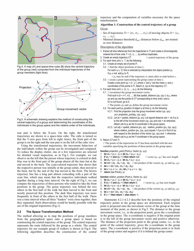
The attributes that are attached to the positions of the central trajectory include the statistical summaries of the individuals’ distances to the group center and the deviations of their movement directions from the group movement vector: minimum, maximum, median, quartiles, and mean. These attributes allow the investigation of the group movement at the level of the group as a whole [16]. For example, Figures 6 and 7 represent different positional attributes of the central trajectory by proportional line width. This visualization technique is applied on a map and in a space-time cube. Figure 6 shows the variation of the third quartile of the distances of the group members to the group centre along the route. We can see where the people walked compactly (this is where the line is thin) and where the group was more dispersed (the line is thick). In a similar way, Figure 7 shows the variation of the third quartile of the direction deviations from the overall group movement vector. The thick line segments correspond to high deviations.

2.3 Data Analysis in Group Space

The coordinates of the trajectory points in the group space, which result from Algorithm 1, are used for representing the trajectories in the group space as shown in Figs. 2 and 3. Trajectories can be

interactively explored using coordinated multiple views where the trajectories are shown in the original (geographic) spatial context, in the group space, and on temporal displays, such as a temporal bar chart (Fig.9, C and D). The multiple views are coordinated through synchronous highlighting of corresponding elements, uniform reaction to interactive dynamic filtering, synchronous animation, and other standard techniques. A specific coordination technique for this kind of data is propagation of selected spatio-temporal points of trajectories: when the mouse cursor is placed over a display element representing some trajectory point in one of the views, the point selection is propagated over all views. In the response, each view marks the location of the selected point within its own display area in its specific way. User interaction with coordinated multiple views of trajectories is demonstrated in supplementary video 1.

Examples of more sophisticated ways of analysis are shown in Figs. 8 and 9. Fig.8 illustrates the application of clustering to time intervals characterized in terms of the individuals’ positions in the group space. We have divided the time span of the data into intervals

Fig.8. Time graphs show the temporal variation of the Y- and X-positions of the individuals in the group space. The background coloring reflects the results of clustering 15-second time intervals according to the positions of the group members in the group space.

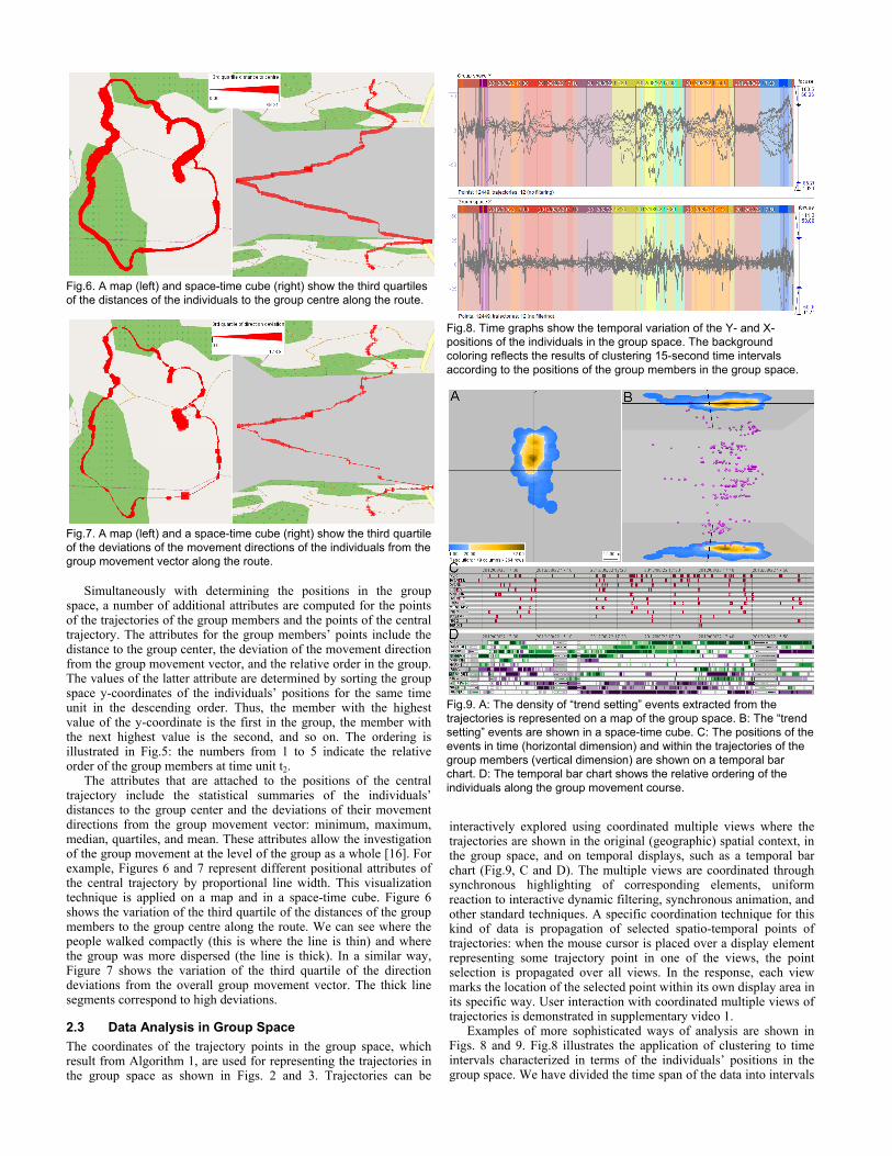
Fig.9. A: The density of “trend setting” events extracted from the trajectories is represented on a map of the group space. B: The “trend setting” events are shown in a space-time cube. C: The positions of the events in time (horizontal dimension) and within the trajectories of the group members (vertical dimension) are shown on a temporal bar chart. D: The temporal bar chart shows the relative ordering of the individuals along the group movement course.

Fig.6. A map (left) and space-time cube (right) show the third quartiles of the distances of the individuals to the group centre along the route.

Fig.7. A map (left) and a space-time cube (right) show the third quartile of the deviations of the movement directions of the individuals from the group movement vector along the route.

of the length of 15 seconds. For each interval, the mean x- and y-positions of each walker have been computed. The mean positions of all individuals have been used in the clustering as feature vectors characterizing the time intervals. As a result, each cluster consists of time intervals in which the group members had similar relative positions with respect to each other. For the visualization of the clustering results, the clusters are assigned different colors in a way described in paper [32]. Fig.8 represents the result of k-means clustering with k=12; other clustering methods could be applied as well. The cluster colors are used to paint the background in the time graphs showing the temporal variation of the y- and x-coordinates of the individuals in the group space (each line corresponds to one individual). The light pink shade marks the time periods when the group was compact in both y- and x-dimensions, i.e., the length and the width, the light shades of red and violet correspond to stretching in the length while staying compact in the width, yellow and orange mark the periods when the group was stretched in both length and width. The alternating stripes of yellow and cyan mark the period when the group was highly stretched in the length, and a few individuals walking at the rear of the group occurred to be sometimes left (cyan), sometimes right (yellow) of the group movement vector. The shades of blue at the end of the time line correspond to high stretching in the y-dimension and moderate stretching in the x-dimension; the arrangement of the walkers was, evidently, different from that in the previous periods.

Figure 9 illustrates the analysis of the leadership and “trend setting” relations between the group members. We adhere to the definition of leadership as being in front of the group [25] and “trend setting” as being “copied” by others after a time lag [17]. More specifically, we assume that “trend setting” at time unit t occurs when an individual takes a movement direction significantly deviating from the direction of the group but at some moment t+Δ the group takes the same direction as the individual at time t.

From the trajectories, we extract “trend setting” events by means of interactive filtering of the trajectory positions according to the values of positional attributes, as described in paper [33]. We set the following filter conditions: a trajectory point is selected if (1) its distance to the group center is not more than 25m, (2) the current movement direction deviates from the current group’s direction by at least 30°, (3) the minimal difference of the current direction from the group’s direction in the next 30 seconds is at most 5°, and (4) the minimal difference of the current direction from the group’s direction in the past 30 seconds is at least 15°. Condition (4) is added for excluding the cases when individuals adjust their movement directions to the group’s directions in the previous moments.

The points satisfying the filter conditions are extracted from the trajectories and treated as spatial events [33]. The map in Fig.9A shows the density distribution of the extracted 210 “trend setting” events in the group space. It can be seen that the highest density (shades of brown) is attained in the front part of the group space. The density is somewhat higher to the left of the y-axis than to the right. The space-time cube in Fig.9B shows the distribution of the “trend setting” events in the group space and in time. The events are represented by purple balls. The temporal bar chart in Fig.9C shows the temporal positions of the events in the trajectories from which they have been extracted. The trajectory of each group member is represented by a bar; the horizontal dimension represents time.

For investigating the leadership, the temporal bar chart in Fig.9D represents the relative ordering of the individuals along the group movement vector by coloring of bar segments. The shades of green, from dark to light, encode the first three positions, and the shades of violet, from light to dark, the last three positions. White corresponds to the central six positions. The trajectory segments corresponding to the group stops are filtered out. As in Fig.9C, the bars are ordered according to the descending counts of the trend setting events extracted from the trajectories. It can be seen that the most frequent “trend setters”, whose bars are at the top of the display, also occupied the leading positions in the group for long time periods. Numerically, 157 out of the 210 “trend setting” events (75%)

occurred on the relative positions 1 to 3 in the group. Hence, it can be concluded that this group was led by the individuals moving in front of the group.

3 CASE STUDY: SAVANNAH BABOONS

3.1 Data and Research Questions

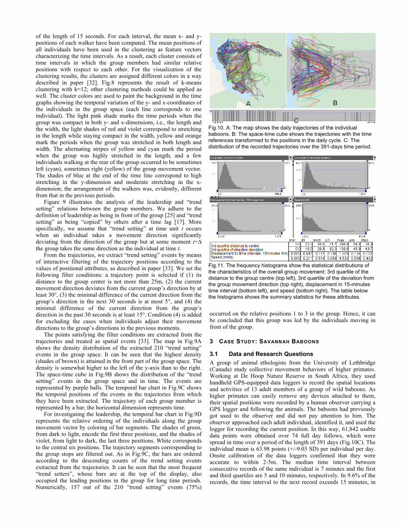
A group of animal ethologists from the University of Lethbridge (Canada) study collective movement behaviors of higher primates. Working at De Hoop Nature Reserve in South Africa, they used handheld GPS-equipped data loggers to record the spatial locations and activities of 13 adult members of a group of wild baboons. As higher primates can easily remove any devices attached to them, their spatial positions were recorded by a human observer carrying a GPS logger and following the animals. The baboons had previously got used to the observer and did not pay attention to him. The observer approached each adult individual, identified it, and used the logger for recording the current position. In this way, 61,842 usable data points were obtained over 74 full day follows, which were spread in time over a period of the length of 391 days (Fig.10C). The individual mean is 63.98 points (+/-9.03 SD) per individual per day. Onsite calibration of the data loggers confirmed that they were accurate to within 2-5m. The median time interval between consecutive records of the same individual is 7 minutes and the first and third quartiles are 5 and 10 minutes, respectively. In 9.6% of the records, the time interval to the next record exceeds 15 minutes, in

Fig.10. A: The map shows the daily trajectories of the individual baboons. B: The space-time cube shows the trajectories with the time references transformed to the positions in the daily cycle. C: The distribution of the recorded trajectories over the 391-days time period.

Fig.11. The frequency histograms show the statistical distributions of the characteristics of the overall group movement: 3rd quartile of the distance to the group centre (top left), 3rd quartile of the deviation from the group movement direction (top right), displacement in 15-minutes time interval (bottom left), and speed (bottom right). The table below the histograms shows the summary statistics for these attributes.

4.5% of the records, it exceeds 20 minutes, and the maximum is 213 minutes. Hence, the temporal resolution of the data is rather low.

The trajectories of the baboons in the geographical space are shown on a map and in a space-time cube in Fig.10A and B. In the space-time cube, the original time references of the trajectory points have been transformed to the positions within the daily cycle [34]. The trajectory lines are colored according to the observation dates.

By analyzing the collected data, the animal researchers wish to understand how individual differences that affect local patterns of interaction can have global effects on group organization, where these can change the process by which decisions are made and drive the emergence of particular roles, such as ‘leaders’.

Although the analysis was carried out with an active participation of the domain experts, the latter did not directly apply all the analysis tools by themselves but used interactive visual displays representing results of data transformations, computations, classifications, and other analytical operations performed by the method developers.

3.2 Analysis at the Group Level

By applying Algorithm 1 to the baboons’ trajectories, we construct the central trajectory of the group for each observation day; hence, we obtain 74 central trajectories. The central trajectories and the characteristics of the group movement along the routes could be explored using maps and space-time cube displays, as illustrated in Figs. 6 and 7. However, the particular route and movement characteristics of the baboon group in each day are not of much interest. The animal researchers wish to study the group behavior at a more general level. For this purpose, it is appropriate to look at the statistics of the group movement characteristics attached to the segments of the central trajectories. Thus, the frequency histograms and the table in Fig. 11 show the statistical distributions of the values of the following attributes: 3rd quartile of the distance to the group centre, 3rd quartile of the deviation from the group movement direction, displacement in 15-minutes time interval, and speed.

The group movement characteristics can be used for classifying the segments of the central trajectories according to the types of movement behaviors. Besides stops, the observers of the animals noticed two different types of group movement: “marches” and “meanders”. The former involve fast, highly coordinated movement along a common course. The latter involve slow, less coordinated, non-directional movements. The observers cannot say precisely what criteria distinguish different movement types. Therefore, we have roughly classified the trajectory segments into marches, meanders, and stops taking into account the statistical distributions of the movement characteristics and using interactive visual displays. Specifically, we looked at the spatial extents of the segments on a map (stops need to have small extents and marches need to be long) and at the inclinations of the segments in a space-time cube (stops need to be nearly vertical and marches close to horizontal). As a result, segments were classified as stops when the displacement in 15 minutes was less than 50m and the speed less than 0.2km/h, as marching when the displacement in 15 minutes was not less than 100m, and as meandering otherwise. Of course, the classification results need to be treated as approximations of actual types of movement behaviors rather than exact portrayals.

3.3 Analysis at the Individual Level

Analogously to the overall group movement, the researchers are not interested in detailed examination of the movements of each group member in each day but they want to obtain a general portrait of the movement behavior of each individual, being particularly interested in determining individual’s role and/or degree of influence.

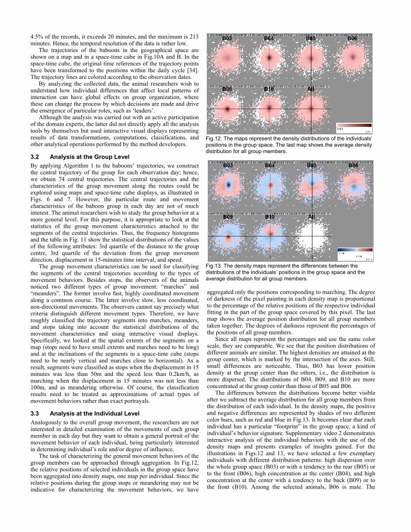
The task of characterizing the general movement behaviors of the group members can be approached through aggregation. In Fig.12, the relative positions of selected individuals in the group space have been aggregated into density maps, one map per individual. Since the relative positions during the group stops or meandering may not be indicative for characterizing the movement behaviors, we have

aggregated only the positions corresponding to marching. The degree of darkness of the pixel painting in each density map is proportional to the percentage of the relative positions of the respective individual fitting in the part of the group space covered by this pixel. The last map shows the average position distribution for all group members taken together. The degrees of darkness represent the percentages of the positions of all group members.

Since all maps represent the percentages and use the same color scale, they are comparable. We see that the position distributions of different animals are similar. The highest densities are attained at the group center, which is marked by the intersection of the axes. Still, small differences are noticeable. Thus, B03 has lower position density at the group center than the others, i.e., the distribution is more dispersed. The distributions of B04, B09, and B10 are more concentrated at the group center than those of B05 and B06.

The differences between the distributions become better visible after we subtract the average distribution for all group members from the distribution of each individual. In the density maps, the positive and negative differences are represented by shades of two different color hues, such as red and blue in Fig.13. It becomes clear that each individual has a particular “footprint” in the group space, a kind of individual’s behavior signature. Supplementary video 2 demonstrates interactive analysis of the individual behaviors with the use of the density maps and presents examples of insights gained. For the illustrations in Figs.12 and 13, we have selected a few exemplary individuals with different distribution patterns: high dispersion over the whole group space (B03) or with a tendency to the rear (B05) or to the front (B06), high concentration at the center (B04), and high concentration at the center with a tendency to the back (B09) or to the front (B10). Among the selected animals, B06 is male. The

Fig.12. The maps represent the density distributions of the individuals’ positions in the group space. The last map shows the average density distribution for all group members.

Fig.13. The density maps represent the differences between the distributions of the individuals’ positions in the group space and the average distribution for all group members.

spatial footprint of B06 is similar to the patterns of the other males in the group and dissimilar to the patterns of all females.

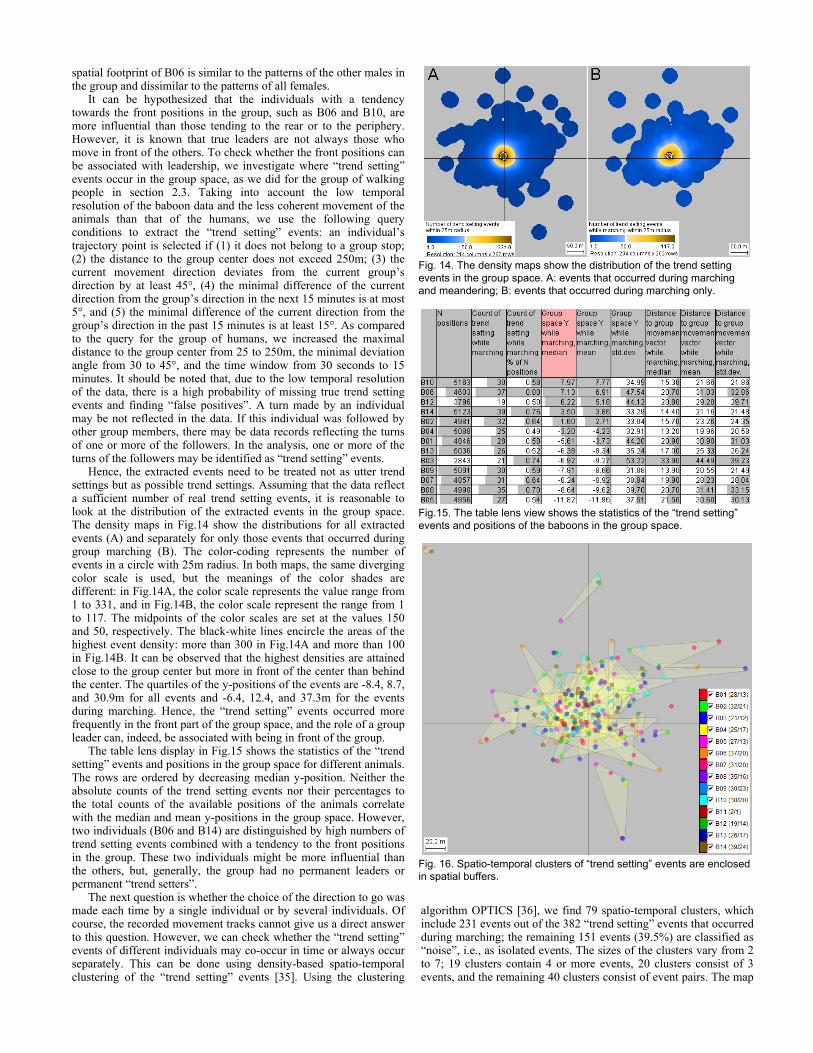
It can be hypothesized that the individuals with a tendency towards the front positions in the group, such as B06 and B10, are more influential than those tending to the rear or to the periphery. However, it is known that true leaders are not always those who move in front of the others. To check whether the front positions can be associated with leadership, we investigate where “trend setting” events occur in the group space, as we did for the group of walking people in section 2.3. Taking into account the low temporal resolution of the baboon data and the less coherent movement of the animals than that of the humans, we use the following query conditions to extract the “trend setting” events: an individual’s trajectory point is selected if (1) it does not belong to a group stop; (2) the distance to the group center does not exceed 250m; (3) the current movement direction deviates from the current group’s direction by at least 45°, (4) the minimal difference of the current direction from the group’s direction in the next 15 minutes is at most 5°, and (5) the minimal difference of the current direction from the group’s direction in the past 15 minutes is at least 15°. As compared to the query for the group of humans, we increased the maximal distance to the group center from 25 to 250m, the minimal deviation angle from 30 to 45°, and the time window from 30 seconds to 15 minutes. It should be noted that, due to the low temporal resolution of the data, there is a high probability of missing true trend setting events and finding “false positives”. A turn made by an individual may be not reflected in the data. If this individual was followed by other group members, there may be data records reflecting the turns of one or more of the followers. In the analysis, one or more of the turns of the followers may be identified as “trend setting” events.

Hence, the extracted events need to be treated not as utter trend settings but as possible trend settings. Assuming that the data reflect a sufficient number of real trend setting events, it is reasonable to look at the distribution of the extracted events in the group space. The density maps in Fig.14 show the distributions for all extracted events (A) and separately for only those events that occurred during group marching (B). The color-coding represents the number of events in a circle with 25m radius. In both maps, the same diverging color scale is used, but the meanings of the color shades are different: in Fig.14A, the color scale represents the value range from 1 to 331, and in Fig.14B, the color scale represent the range from 1 to 117. The midpoints of the color scales are set at the values 150 and 50, respectively. The black-white lines encircle the areas of the highest event density: more than 300 in Fig.14A and more than 100 in Fig.14B. It can be observed that the highest densities are attained close to the group center but more in front of the center than behind the center. The quartiles of the y-positions of the events are -8.4, 8.7, and 30.9m for all events and -6.4, 12.4, and 37.3m for the events during marching. Hence, the “trend setting” events occurred more frequently in the front part of the group space, and the role of a group leader can, indeed, be associated with being in front of the group.

The table lens display in Fig.15 shows the statistics of the “trend setting” events and positions in the group space for different animals. The rows are ordered by decreasing median y-position. Neither the absolute counts of the trend setting events nor their percentages to the total counts of the available positions of the animals correlate with the median and mean y-positions in the group space. However, two individuals (B06 and B14) are distinguished by high numbers of trend setting events combined with a tendency to the front positions in the group. These two individuals might be more influential than the others, but, generally, the group had no permanent leaders or permanent “trend setters”.

The next question is whether the choice of the direction to go was made each time by a single individual or by several individuals. Of course, the recorded movement tracks cannot give us a direct answer to this question. However, we can check whether the “trend setting” events of different individuals may co-occur in time or always occur separately. This can be done using density-based spatio-temporal clustering of the “trend setting” events [35]. Using the clustering

algorithm OPTICS [36], we find 79 spatio-temporal clusters, which include 231 events out of the 382 “trend setting” events that occurred during marching; the remaining 151 events (39.5%) are classified as “noise”, i.e., as isolated events. The sizes of the clusters vary from 2 to 7; 19 clusters contain 4 or more events, 20 clusters consist of 3 events, and the remaining 40 clusters consist of event pairs. The map

Fig. 14. The density maps show the distribution of the trend setting events in the group space. A: events that occurred during marching and meandering; B: events that occurred during marching only.

Fig.15. The table lens view shows the statistics of the “trend setting” events and positions of the baboons in the group space.

Fig. 16. Spatio-temporal clusters of “trend setting” events are enclosed in spatial buffers.

in Fig.16 shows the positions and shapes of the clusters in the group space. To obtain this map, we have built spatial buffers around the event clusters. The buffers are drawn with 25% opacity. The events belonging to the clusters are shown by dots colored according to the individuals that “produced” them. The legend on the right explains the colors and shows for each individual two numbers: the total count of events and the number of events that belong to the clusters.

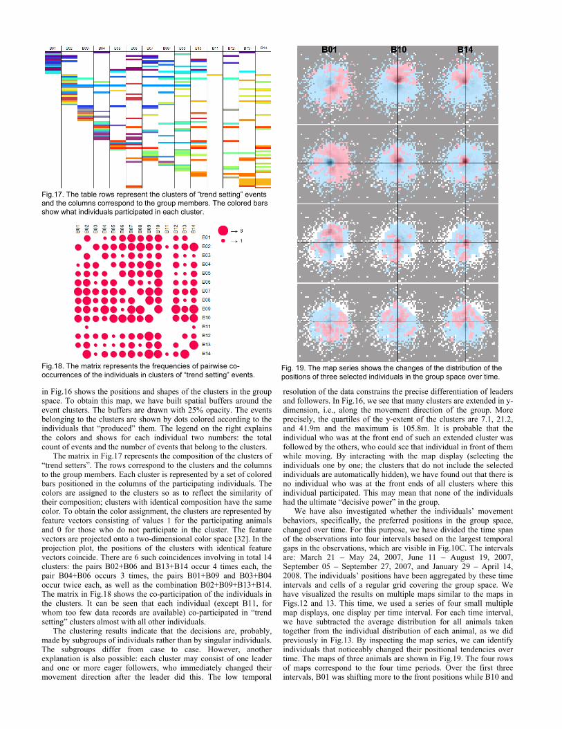
The matrix in Fig.17 represents the composition of the clusters of “trend setters”. The rows correspond to the clusters and the columns to the group members. Each cluster is represented by a set of colored bars positioned in the columns of the participating individuals. The colors are assigned to the clusters so as to reflect the similarity of their composition; clusters with identical composition have the same color. To obtain the color assignment, the clusters are represented by feature vectors consisting of values 1 for the participating animals and 0 for those who do not participate in the cluster. The feature vectors are projected onto a two-dimensional color space [32]. In the projection plot, the positions of the clusters with identical feature vectors coincide. There are 6 such coincidences involving in total 14 clusters: the pairs B02+B06 and B13+B14 occur 4 times each, the pair B04+B06 occurs 3 times, the pairs B01+B09 and B03+B04 occur twice each, as well as the combination B02+B09+B13+B14. The matrix in Fig.18 shows the co-participation of the individuals in the clusters. It can be seen that each individual (except B11, for whom too few data records are available) co-participated in “trend setting” clusters almost with all other individuals.

The clustering results indicate that the decisions are, probably, made by subgroups of individuals rather than by singular individuals. The subgroups differ from case to case. However, another explanation is also possible: each cluster may consist of one leader and one or more eager followers, who immediately changed their movement direction after the leader did this. The low temporal

resolution of the data constrains the precise differentiation of leaders and followers. In Fig.16, we see that many clusters are extended in y-dimension, i.e., along the movement direction of the group. More precisely, the quartiles of the y-extent of the clusters are 7.1, 21.2, and 41.9m and the maximum is 105.8m. It is probable that the individual who was at the front end of such an extended cluster was followed by the others, who could see that individual in front of them while moving. By interacting with the map display (selecting the individuals one by one; the clusters that do not include the selected individuals are automatically hidden), we have found out that there is no individual who was at the front ends of all clusters where this individual participated. This may mean that none of the individuals had the ultimate “decisive power” in the group.

We have also investigated whether the individuals’ movement behaviors, specifically, the preferred positions in the group space, changed over time. For this purpose, we have divided the time span of the observations into four intervals based on the largest temporal gaps in the observations, which are visible in Fig.10C. The intervals are: March 21 – May 24, 2007, June 11 – August 19, 2007, September 05 – September 27, 2007, and January 29 – April 14, 2008. The individuals’ positions have been aggregated by these time intervals and cells of a regular grid covering the group space. We have visualized the results on multiple maps similar to the maps in Figs.12 and 13. This time, we used a series of four small multiple map displays, one display per time interval. For each time interval, we have subtracted the average distribution for all animals taken together from the individual distribution of each animal, as we did previously in Fig.13. By inspecting the map series, we can identify individuals that noticeably changed their positional tendencies over time. The maps of three animals are shown in Fig.19. The four rows of maps correspond to the four time periods. Over the first three intervals, B01 was shifting more to the front positions while B10 and

Fig.17. The table rows represent the clusters of “trend setting” events and the columns correspond to the group members. The colored bars show what individuals participated in each cluster.

Fig.18. The matrix represents the frequencies of pairwise co-occurrences of the individuals in clusters of “trend setting” events.

Fig. 19. The map series shows the changes of the distribution of the positions of three selected individuals in the group space over time.

B14 were shifting from the front positions to the center and back of the group space. In the fourth interval, the patterns are again similar to those in the first interval, which suggests that the behavioral changes could be seasonal.

3.4 Judgments of Domain Experts

The domain experts got very enthusiastic about what they could see on the visual displays in the course of the study. One of the insights was that the animals have tendencies to certain positions in the group space, which are related to the sex, social rank, and reproductive state (fertile periods; pregnancy; lactation) of the animals. Currently, the ethologists perform statistical analysis of the data to verify the findings, with the aim to publish the results in domain literature.

Regarding the methods and tools used in the study, the experts’ opinion is that these are extremely valuable means of probing the decision rules by which collective animals coordinate their movements. If one can identify the local rules used by animals to maintain, increase or decrease distance to particular others, one can then investigate how the aggregation of these local rules gives rise to overall patterns of movement within a group and by the group as a whole. To date, such studies have only been conducted under highly artificial conditions on smaller-brained organisms. With the development of these new techniques, the researchers will be able to test whether large-brained, wild-living animals similarly use simple local rules that give rise to complex coordinated movement, or whether it is necessary to consider the possibility that primate decision-making is more complex. Although a clear-cut answer has not been obtained yet, the new methods have brought the researchers much closer to it than it was possible before.

The experts appreciate the way in which temporal dynamics are built into the visualizations, so that patterns over time are made highly visible (in particular, in depictions using the space-time cube), with respect to group movements as a whole over time. The identification of ‘marches’ and ‘meanders’ within and across days is highly useful for testing hypotheses relating to patterns of range use in relation to individual decision making. The ability to track the relative positioning of different animals within and across days is even more crucial because it allows a more refined assessment of what constitutes ‘leadership’ in such groups. It is clear that leadership reflects differing degrees of ‘influence’ across individuals, and is not merely the result of spatial positioning. The measure of ‘trend-setting’ is useful in this respect, allowing temporal as well as spatial contingency to be assessed in a precise quantitative fashion.

The ability to obtain spatially explicit data from habituated social animals is driving a new generation of questions about the consequences and correlates of gregariousness, for which a new generation of analytical techniques is needed. One central issue concerns the extent to which one animal can influence the use of space by others and thereby structure the group’s activities. Most analyses have concentrated on leadership because these are easy data to extract. At the same time, however, such analyses ignore different and potentially more subtle influences that may well interact with one another. In addition to being scale-free, which will greatly facilitate direct comparisons across study sites and species, the application of the methods outlined here to wild primates has already revealed such novel interactions that will be central to our more formal analysis of socio-spatial architecture.

4 DISCUSSION AND CONCLUSION

Algorithm 1 produces two major results: the central trajectory of a group and the coordinates of the group members in the group space. Additionally, it computes a number of attributes referring to the positions of the central trajectory and of the individual trajectories of the group members. The central trajectory and the associated positional attributes, which reflect the overall characteristics of the group (dispersion in space, variation of the members’ movement direction, spatial extents along and across the movement direction, etc.), are used for analyzing the group movement at the level of the

group as a whole, including the change of the group’s position in space and the evolution of its spatial footprint. The coordinates of the members in the group space and the associated positional attributes (distance from the group center, deviation from the group’s movement direction, relative order with respect to the other members, etc.) are used for analyzing the group movement at the level of individual group members. Hence, our approach supports the three levels of analysis defined by Wood and Galton [13]-[16].

The worth of the coordinate transformation to the group space is that it enables abstraction from the absolute positions of the moving objects in the geographical space and focusing on their relative positions with respect to each other, regardless of where the whole group is in the original space. The approach is unique; none of the previously existing techniques would enable gaining the same kind of knowledge about the behaviors of individuals within a group as is possible by exploiting the space transformation.

A good feature of both results of Algorithm 1 is that the variety of existing visual analytics methods designed for movement data [7] can be applied to the central trajectories and to the trajectories of the individuals mapped onto the group space. We have demonstrated the use of methods for analysis of relatively small datasets at a high level of detail (section 2.3) and scalable methods for analysis at a more general level. The scalable methods focus on spatial, temporal, and statistical distributions and involve spatial and temporal aggregation, event extraction, clustering, and statistical summarization. Algorithm 1 itself is scalable to large datasets since it has linear computational complexity (all computations can be done in a single scan of the set of object positions) and does not require all data to be loaded in RAM at once. At each step, it only needs two consecutive positions from each trajectory; hence, the data can be processed by portions.

Besides being scalable, the presented methodology is also robust with respect to the temporal resolution of the data. It worked well both for the group walk data with fine temporal resolution and for the baboon movement data with low temporal resolution. Algorithm 1 has no inherent limitations concerning the temporal resolution of the data. The resolution only limits the level of detail that is possible in the analysis of both original and transformed data.

However, an essential requirement is synchronization between the positions of the individuals: to find the center of a group at a time moment t, it is necessary to know the positions of all group members at the moment t. Hence, either the positions need to be measured and recorded simultaneously, or the data must allow interpolation [9].

The suggested approach is applicable to data reflecting group movement, when multiple objects move together as a single unit, which gives the possibility to identify the center and movement direction of this unit. The approach is not applicable to independent movements of multiple objects, when there is no common movement direction. The approach is primarily oriented to movement in a two-dimensional metric space, such as geographic space. Technically, it can be applied to data referring to an abstract space, such as a space of value combinations of two numeric attributes; however, the distances and directions in such a space may be difficult to interpret.

Possible application domains of the methodology include, besides the research of movement behaviors of collective animals, analysis of movements in various race sports, where the racers move together, and their relative positions change along the way. Algorithm 1 and the following analysis of its results can also be applied to moving groups (‘flocks’, ‘moving clusters’, ‘herds’, etc.) identified by dedicated computational methods [3][11][12][22][23][24].

The application of the methodology to animal movement data has demonstrated a high utility of the invented space transformation for the investigation of individual behavioral differences. In the future, we plan to devise other space transformations suitable for different types of data and productive for various specific kinds of analysis.

ACKNOWLEDGMENTS

The authors gratefully acknowledge The Leakey Foundation for funding the baboon data collection.

REFERENCES

[1] R.H. Güting, M. Schneider. Moving Objects Databases. Morgan Kaufmann, 2005.

[2] D. Pfoser, C.S. Jensen, and Y. Theodoridis. Novel approaches to the indexing of moving object trajectories. Proc. Int. Conf. Very Large Databases VLDB 2000, 395-406, 2000.

[3] P. Laube. Progress in movement pattern analysis. Behavior Monitoring and Interpretation - Ambient Assisted Living, B. Gottfried and H. Aghajan, eds., IOS Press, pp. 43-71, 2009.

[4] Y. Zheng and X. Zhou (eds.) Computing with Spatial Trajectories. Springer, 2011.

[5] F.Giannotti and D.Pedreschi (eds.) Mobility, Data Mining and Privacy - Geographic Knowledge Discovery. Springer, 2008.

[6] D. Taniar and L. Iwan. Exploring Advances in Interdisciplinary Data Mining and Analytics. IGI Global, 2011.

[7] G. Andrienko, N. Andrienko, P. Bak, D. Keim, S. Kisilevich, and S. Wrobel. A Conceptual Framework and Taxonomy of Techniques for Analyzing Movement. Journal of Visual Languages and Computing, 22(4):251-256, 2011.

[8] N. Andrienko and G. Andrienko. Visual analytics of movement: An overview of methods, tools and procedures. Information Visualization, 12(1): 3-24, 2013

[9] G. Andrienko, N. Andrienko, P. Bak, D. Keim, and S. Wrobel. Visual Analytics of Movement. Springer, 2013.

[10] S. Dodge, R. Weibel, and A.-K. Lautenschütz. Towards a taxonomy of movement patterns. Information Visualization, 7:240–252, 2008.

[11] M. Benkert, J. Gudmundsson, F. Hübner, and T. Wolle. Reporting flock patterns. Lecture Notes in Computer Science 4168: Proc. 14th Annual European Symposium on Algorithms (ESA'06), Y. Azar, ed., Berlin: Springer-Verlag, pp. 660-671, 2006

[12] Y. Huang, C. Chen, and P. Dong. Modelling herds and their evolvements from trajectory data. Lecture Notes in Computer Science 5266: Proc. 5th international conference on Geographic Information Science (GIScience’10), Springer-Verlag, pp. 90–105, 2008

[13] Z. Wood and A. Galton. A taxonomy of collective phenomena. Applied Ontology, 4(3-4):267-292, 2009

[14] Z. Wood and A. Galton. Classifying collective motion. Behaviour Monitoring and Interpretation - BMI: Smart Environments, B. Gottfried and H. Aghajan, eds., Amsterdam: IOS Press, pp. 129-155, 2009.

[15] Z. Wood and A. Galton. Zooming in on collective motion. Spatio-Temporal Dynamics, Proc. Workshop 21, 19th European Conference on Artificial Intelligence, M. Bhatt, H. Guesgen and S. Hazarika, pp. 25-30, 2010.

[16] Z. Wood, “Detecting and identifying collective phenomena within movement data”, PhD thesis, Dept. of Computer Science, Univ. of Exeter, UK, 2011. URI: http://hdl.handle.net/10036/3293

[17] P. Laube, S. Imfeld, and R. Weibel. Discovering relative motion patterns in groups of moving point objects. International Journal of Geographical Information Science, 19(6):639–668, 2005.

[18] C. Reynolds. Flocks, herds and schools: A distributed behavioral model. Proc. 14th annual conf. Computer graphics and interactive techniques, pp. 25–34, 1987

[19] R. Eftimie, G. de Vries, M.A. Lewis, and F. Lutscher. Modeling group formation and activity patterns in self-organizing collectives of individuals. Bulletin of Mathematical Biology, 69:1537–1565, 2007

[20] H. Jeung, M.L. Yiu, and C.S. Jensen. Trajectory pattern mining. Y. Computing with Spatial Trajectories, Zheng and X. Zhou (eds.), Springer, pp. 143-177, 2011.

[21] P. Laube, M. van Kreveld, and S. Imfeld. Finding REMO - detecting relative motion patterns in geospatial lifelines. Developments in Spatial Data Handling, Proc. 11th Int. Symp. Spatial Data Handling, P.F. Fisher, ed., Springer, Heidelberg, pp. 201-214, 2004

[22] J. Gudmundsson, M. van Kreveld, and B. Speckmann. Efficient detection of patterns in 2D trajectories of moving points, Geoinformatica, 11(2):195-215, 2007.

[23] P.Kalnis, N.Mamoulis, S.Bakiras. On discovering moving clusters in spatio-temporal data. Lecture Notes in Computer Science 3633: Advances in spatial and temporal databases, 9th Int. Symp. SSTD 2005,

C. Bauzer Medeiros, M. Egenhofer, and E. Bertino, eds., pp.364-381, 2005

[24] J. Gudmundsson, P. Laube, and T. Wolle. Computational movement analysis. Springer Handbook of Geographic Information, W. Kresse and D. Danko, eds., Springer, Berlin-Heidelberg, pp. 725-741, 2012.

[25] M. Andersson, J. Gudmundsson, P. Laube, and T. Wolle. Reporting leaders and followers among trajectories of moving point objects. Geoinformatica, 12(4): 497-528, 2008.

[26] D. J. T. Sumpter. Collective Animal Behavior, Princeton University Press, Princeton, 2010.

[27] M. Nagy, Z. Ákos, D. Biro, and T. Vicsek. Hierarchical group dynamics in pigeon flocks. Nature, 464: 890-893, 8 April 2010.

[28] T. von Landesberger, S. Bremm, T. Schreck, and D. Fellner. Feature-based automatic identification of interesting data segments in group movement data. Information Visualization, 2013.

[29] L. Wilkinson, A. Anand, and R. Grossman. Graph-theoretic scagnostics. Proc. IEEE Symp. Information Visualization, pp. 157-164, 2005

[30] M.-J. Kraak. The space-time cube revisited from a geovisualization perspective. Proc. 21st Int. Cartographic Conf., pp. 1988-1995, 2003

[31] T. Kapler and W. Wright. GeoTime information visualization, Information Visualization, 4(2): 136-146, 2005

[32] N. Andrienko and G. Andrienko. A visual analytics framework for spatio-temporal analysis and modelling. Data Mining and Knowledge Discovery, 27(1): 55-83, 2013.

[33] G. Andrienko, N. Andrienko, and M. Heurich. An event-based conceptual model for context-aware movement analysis. International Journal Geographical Information Science, 25(9): 1347-1370, 2011.

[34] G. Andrienko and N. Andrienko. Poster: Dynamic time transformation for interpreting clusters of trajectories with space-time cube. Proc. IEEE symp. Visual Analytics Science and Technology (VAST 2010), 213-214, 2010.

[35] G. Andrienko and N. Andrienko. Interactive Cluster Analysis of Diverse Types of Spatiotemporal Data. ACM SIGKDD Explorations, 11(2): 19-28, 2009.

[36] M. Ankerst, M. Breunig, H-P. Kriegel, and J. Sander. OPTICS: Ordering points to identify the clustering structure. Proc. ACM SIGMOD Int. Conf. Management of Data (SIGMOD'99), Philadelphia, USA, 49-60, 1999.