southern headwaters at risk project: a multi-species ... · a multi-species conservation strategy...
TRANSCRIPT
The Southern Headwaters At Risk Project:A Multi-Species Conservation Strategy for
the Headwaters of the Oldman River
Volume 2
Species Selection and Habitat Suitability Index Models
Alberta Species at Risk Report No. 90
The Southern Headwaters At Risk Project: A Multi-Species Conservation Strategy
for the Headwaters of the Oldman River
Volume 2
Species Selection and Habitat Suitability Index Models
Compiled and Edited by François Blouin, Brad N. Taylor, and Richard W. Quinlan
Alberta Species at Risk Report No. 90
November 2004

Publication No. I/162 ISBN No. 0-7785-3566-5 (Printed Edition) ISBN No. 0-7785-3567-3 (On-line Edition) ISSN No. 1496-7219 (Printed Edition) ISSN No. 1496-7146 (On-line Edition) For copies of this report, contact: Information Centre- Publications Alberta Environment/ Alberta Sustainable Resource Development Main Floor, Great West Life Building 9920- 108 Street Edmonton, Alberta, Canada T5K 2M4 Telephone: (780) 422-2079
OR Visit our web site at: http://www3.gov.ab.ca/srd/fw/riskspecies/. Suggested citation formats:
Entire Report Blouin, F., B.N.Taylor, and R.W.Quinlan (eds). 2004. The southern headwaters at risk project: A multi-species conservation strategy for the headwaters of the Oldman River. Volume 2: Species Selection and Habitat Suitability Models. Alberta Sustainable Resource Development, Fish and Wildlife Division, Alberta Species at Risk Report No. 90, Edmonton, AB.
Individual Habitat Suitability Index Models Smith, C., and D. Paton. 2004. Habitat suitability index model for the harlequin duck (Histrionicus histrionicus). Pp. 13-26 in Blouin, F., B.N.Taylor, and R.W.Quinlan (eds). 2004. The southern headwaters at risk project: A multi-species conservation strategy for the headwaters of the Oldman River. Volume 2: Species Selection and Habitat Suitability Models. Alberta Sustainable Resource Development, Fish and Wildlife Division, Alberta Species at Risk Report No. 90, Edmonton, AB.

i
TABLE OF CONTENTS Page
APPENDICES .................................................................................................................... ii LIST OF TABLES............................................................................................................. iii LIST OF FIGURES ........................................................................................................... iv LIST OF MAPS ............................................................................................................... viii AKNOWLEDGEMENTS.................................................................................................. ix EXECUTIVE SUMMARY ................................................................................................ x INTRODUCTION .............................................................................................................. 1 STUDY AREA ................................................................................................................... 3 METHODS ......................................................................................................................... 4
Focal Species Selection Process ..................................................................................... 4 Habitat Suitability Index Modeling ................................................................................ 6
LITTERATURE CITED..................................................................................................... 8 HABITAT SUITABILITY INDEX MODELS:
Harlequin Duck (Histrionicus histrionicus)..................................................... 13 Ferruginous Hawk (Buteo regalis).................................................................. 27 Prairie Falcon (Falco mexicanus) ..................................................................... 36 Sharp-tailed Grouse (Tympanuchus phasianellus) ......................................... 42 Long-Billed Curlew (Numenius americanus) ................................................. 51 Pileated Woodpecker (Dryocopus pileatus).................................................... 57 Clark�s Nutcracker (Nucifraga columbiana) ................................................... 73 Sprague�s Pipit (Anthus spragueii) ................................................................... 82 Loggerhead Shrike (Lanius ludovicianus excubitorides) ................................ 91 Vagrant Shrew (Sorex vagrans)........................................................................ 99 Grizzly Bear (Ursus arctos) ............................................................................ 108 Wolverine (Gulo gulo)..................................................................................... 115 Long-Toed Salamander (Ambystoma macrodactylum) ................................ 136 Western Toad (Bufo boreas) ........................................................................... 148 Northern Leopard Frog (Rana pipiens) ........................................................ 160

ii
APPENDICES
Page Appendix 5. 1. Histograms of sharp-tailed grouse habitat variables for occupied sites
(sharp-tailed grouse lek sites on the milk river ridge, n=42) and available sites (4219 quarter sections on the milk river ridge).................................... 50
Appendix 7. 1. Relating field-measured stand dbh to the Alberta Vegetation Inventory
(AVI) stand origin (modified from Greidanus 2003)................................... 70 Appendix 1. Alberta Natural Heritage Information Centre�s ranking system (modified
from Vujnovic and Gould (2002)). ............................................................ 172 Appendix 2. Focal species selection matrix (used as a guide in the final selection of SAR
management species).. ............................................................................... 173 Appendix 3. Species at risk, may be at risk, or data deficient in the SHARP area......... 174

iii
LIST OF TABLES Page
Table 1. 1. Weight and rationale for focal species selection criteria. ............................... 5 Table 1. 2. Focal species for the SHARP area. ................................................................. 5 Table 3. 1. Soil texture classifications1........................................................................... 30 Table 9. 1. Characteristics of nest sites (n=47) in Saskatchewan (Sutter 1997)............. 83 Table 12. 1. Total bears in each HPI category, with mean HPI value listed on the far
right.. .......................................................................................................... 110

iv
LIST OF FIGURES Page
Figure 1. 1. Southern Headwaters At Risk Project study area............................................ 3 Figure 1. 2. Extent of coverage of a) the Alberta Vegetation Inventory database, b) the
Native Prairie Vegetation Inventory database, and c) the Agricultural Region of Alberta Soil Inventory Database in the SHARP study area. ...................... 7
Figure 2. 1. Habitat suitability index for natural region (V1) for the harlequin duck. ...... 17 Figure 2. 2. Habitat suitability index for hydrographic feature type (V2) for harlequin
duck............................................................................................................... 18 Figure 2. 3. Habitat suitability index for riparian vegetation cover variable (V3) for
harlequin duck............................................................................................... 18 Figure 2. 4. Habitat suitability index for distance from suitable hydrographic feature
variable (V4) for harlequin duck. .................................................................. 19 Figure 2. 5. Habitat suitability index for distance from roads or railroads variable (V5) for
harlequin duck............................................................................................... 19 Figure 3. 1. Percent native grass habitat suitability index for the ferruginous hawk........ 30 Figure 3. 2. Soil texture classification habitat suitability index for the ferruginous hawk30 Figure 3. 3. Ecoregion habitat suitability index for the ferruginous hawk ....................... 31 Figure 3. 4. Percent Trees and Shrubs habitat suitability index for the ferruginous hawk31 Figure 4. 1. Slope habitat suitability index (V1) for the prairie falcon. ............................ 38 Figure 4. 2. Forage habitat suitability index (V3) for the prairie falcon. .......................... 38 Figure 5. 1. Habitat suitability index for native prairie cover class (V1) for the sharp-tailed
grouse ............................................................................................................ 45 Figure 5. 2. Habitat suitability index curve for percent shrub cover (V2) for the sharp-
tailed grouse .................................................................................................. 45 Figure 5. 3.Habitat suitability index curve for percent tree cover (V3) for the sharp-tailed
grouse ............................................................................................................ 46 Figure 6. 1. Habitat suitability index for native graminoids (V1) for the long-billed
curlew............................................................................................................ 52 Figure 6. 2. Habitat suitability for slope (V3) for the long-billed curlew. ........................ 53 Figure 6. 3. Habitat suitability index for percent shrub coverage (V2) for the long-billed
curlew............................................................................................................ 53 Figure 6. 4. Habitat Suitability for treed (V4) areas for the long-billed curlew................ 54 Figure 7. 1. Habitat suitability index for nesting/roosting habitat (V1) for the pileated
woodpecker. .................................................................................................. 60 Figure 7. 2. Example of SI ratings of the �A�density - Douglas-fir leading stratum at
various stand ages for dead conifers. ............................................................ 61 Figure 7. 3. Habitat suitability index for winter-feeding habitat (V2) for the pileated
woodpecker. .................................................................................................. 62

v
Page Figure 7. 4. Example of SI ratings of the �D�density � all stands stratum at various stand
ages for dead conifers. .................................................................................. 63 Figure 7. 5. Habitat suitability index for crown closure (V3) for the pileated woodpecker.
....................................................................................................................... 64 Figure 7. 6. Habitat suitability index for distance from suitable nesting habitat (V4) for the
pileated woodpecker. .................................................................................... 65 Figure 7. 7. Sample graph for the A-denstiy Fd-leading stratum for the breeding habitat.
There is a general trend for the diameter of the dead conifer trees to increase as the stand ages. For stratum with a small number of samples, the P90 tends to be the same value as the maximum, and is plotted underneath its symbol........................................................................................................................ 72
Figure 8. 1. Habitat suitability index for tree species (V1) for the Clark�s nutcracker. .... 77 Figure 8. 2. Habitat suitability index for crown closure (V2) for the Clark�s nutcracker. 77 Figure 8. 3. Habitat suitability index for distance from whitebark pine or limber pine (V3)
for the Clark�s nutcracker........................................................................... 78 Figure 9. 1. Habitat suitability index for percent native grass coverage (V1) for the
Sprague�s pipit............................................................................................ 85 Figure 9. 2. Habitat suitability index for percent tree and shrub cover (V2) for the
Sprague�s pipit............................................................................................ 85 Figure 9. 3. Habitat suitability index for riparian areas (V3) for the Sprague�s pipit. ...... 86 Figure 10. 1. Habitat suitability index for shrub coverage (V1) for the loggerhead shrike
.................................................................................................................... 93 Figure 10. 2. Habitat suitability index for tree coverage (V2) for the loggerhead shrike 93 Figure 10. 3. Habitat suitability index for graminoid coverage (V3) for the loggerhead
shrike .......................................................................................................... 94 Figure 10. 4. Habitat suitability index for slope (V4) for the loggerhead shrike ............. 94 Figure 11. 1. Habitat suitability index for natural subregion (V1) for the vagrant shrew.
.................................................................................................................. 102 Figure 11. 2. Habitat suitability index for ecological moisture regime (V2) for the vagrant
shrew. ....................................................................................................... 102 Figure 11. 3. Habitat suitability index for distance from water (V3) for the vagrant shrew.
.................................................................................................................. 103 Figure 11. 4. Habitat suitability index for crown closure class (V4) for the vagrant shrew.
.................................................................................................................. 104

vi
Page
Figure 12. 1. Suitability index (SI) values for the grizzly bear distance from linear features (after Alberta Environmental Protection 1998)................................ 111
Figure 12. 2. Suitability index (SI) values for the grizzly bear for distance from non-linear human use features (V4) (after Alberta Environmental Protection 1998). These include active and abandoned oil and gas well sites, other facilities (eg. forestry buildings, major towers, etc), cities/towns, ribbon development (golf course, etc.), gravel pits, farmsteads, surface mines, and industrial plant sites........................................................................................................................ 111
Figure 12. 3. Suitability index (SI) valure for distance from cover (V5) (after Alberta Environmental Protection 1998). ................................................................... 112
Figure 13. 1. Suitability index (SI) values for the wolverine for distance from linear
features (after Alberta Environmental Protection 1998)................................ 123 Figure 13. 2. Suitability index (SI) values for the wolverine for distance from non-linear
human use features (V4) (after Alberta Environmental Protection 1998). These include active and abandoned oil and gas well sites, other facilities (eg. forestry buildings, major towers, etc), cities/towns, ribbon development (golf course, etc.), gravel pits, farmsteads, surface mines, and industrial plant sites........................................................................................................................ 124
Figure 13. 3. Wolverine habitat suitability values for the natural subregions (V6) in the SHARP area. .................................................................................................. 125
Figure 14. 1. Habitat Suitability Index for natural subregion (V1) for the long-toed
salamander. .................................................................................................... 139 Figure 14. 2. Habitat suitability index for elevation (V2) for the long-toed salamander.
....................................................................................................................... 140 Figure 14. 3. Habitat suitability index for water body type (V3) for the long-toed
salamander. .................................................................................................... 140 Figure 14. 4. Habitat suitability index for distance from water bodies < 200 ha (V4) for
the long-toed salamander. .............................................................................. 141 Figure 14. 5. Habitat suitability index for cover (V5) for the long-toed salamander. ..... 141 Figure 14. 6. Habitat suitability index for fish presence (V6) for the long-toed salamander.
....................................................................................................................... 142 Figure 14. 7. Habitat suitability index for water body size (V7) for the long-toed
salamander. .................................................................................................... 142 Figure 15. 1. Habitat suitability index for natural subregion (V1) for the western toad. 150 Figure 15. 2. Habitat suitability index for water body type (V2) for the western toad. .. 151 Figure 15. 3. Habitat suitability index for distance from water bodies ≤ 200 ha (V3) for
the western toad. ............................................................................................ 152 Figure 15. 4. Habitat suitability index for cover (V4) for the western toad. ................... 152 Figure 15. 5. Habitat suitability index for fish presence (V5) for the western toad. ....... 153 Figure 15. 6. Habitat suitability index for ecological moisture regime (V6) for the western
toad................................................................................................................. 154

vii
Page Figure 15. 7. Habitat suitability index for distance from water bodies > 200 ha (V7) for
the western toad. ............................................................................................ 154 Figure 15. 8. Habitat suitability index for water body size (V8) for the western toad.... 155 Figure 16. 1. Habitat suitability index for natural subregion (V1) for the northern leopard
frog................................................................................................................. 163 Figure 16. 2. Habitat suitability index for water body type (V2) for the northern leopard
frog................................................................................................................. 164 Figure 16. 3. Habitat suitability index for distance from water bodies ≤ 200 ha (V3) for
the northern leopard frog. .............................................................................. 164 Figure 16. 4. Habitat suitability index for distance from water bodies > 200 ha (V4) for
the northern leopard frog. .............................................................................. 165 Figure 16. 5. Habitat suitability index for presence of fish (V5) for the northern leopard
frog................................................................................................................. 166 Figure 16. 6. Habitat suitability index for water body size (V6) for the northern leopard
frog................................................................................................................. 166

viii
LIST OF MAPS Page
Map 2. 1. Potential habitat for the harlequin duck in the northern section of the SHARP
area................................................................................................................... 24 Map 2. 2. Potential habitat for the harlequin duck in the central section of the SHARP
area................................................................................................................... 25 Map 2. 3. Potential habitat for the harlequin duck in the southern section of the SHARP
area................................................................................................................... 26 Map 3. 1. Potential habitat for the ferruginous hawk in the SHARP area. ....................... 35 Map 4. 1. Potential habitat for the prairie falcon in the SHARP area............................... 41 Map 5. 1. Potential habitat for the sharp-tailed grouse in the SHARP area. .................... 49 Map 6. 1. Potential habitat for the long-billed curlew in the SHARP area....................... 56 Map 7. 1. Potential habitat for the pileated woodpecker in the SHARP area................... 69 Map 8. 1. Potential habitat for the Clark�s nutcracker in the SHARP area. ..................... 81 Map 9. 1. Potential habitat for the Sprague�s pipit in the SHARP area............................ 90 Map 10. 1. Potential habitat for the loggerhead shrike in the SHARP area. .................... 98 Map 11. 1. Potential habitat for the vagrant shrew in the SHARP area. ........................ 107 Map 12. 1. Potential habitat for the grizzly bear in the SHARP area. ............................ 114 Map 13. 1. Potential habitat for the wolverine in the SHARP area. ............................... 135 Map 14. 1. Potential and known habitat for the long-toed salamander in the south end
(south of Highway #3) of the SHARP area. .................................................. 146 Map 14. 2. Potential and known habitat for the long-toed salamander in the north end
(north of Highway #3) of the SHARP area.................................................... 147 Map 15. 1. Potential habitat for the western toad in the north end (north of Highway #3)
of the SHARP area......................................................................................... 158 Map 15. 2. Potential habitat for the western toad in the south end (south of Highway #3)
of the SHARP area......................................................................................... 159 Map 16. 1. Potential habitat for the northern leopard frog in the north end (north of
Highway #3) of the SHARP area................................................................... 170 Map 16. 2. Potential habitat for the northern leopard frog in the south end (south of
Highway #3) of the SHARP area................................................................... 171

ix
AKNOWLEDGEMENTS Funding for the Southern Headwaters At Risk Project was provided through the Alberta Fish and Wildlife Species at Risk Program, the Government of Canada Habitat Stewardship Program for Species at Risk, and the Alberta Conservation Association (ACA). The Southern Headwaters At Risk Project was administered by Brad Taylor of Alberta Conservation Association and Richard Quinlan of Alberta Fish and Wildlife Division (AFWD). The species selection process was made possible through the participation of Carita Bergman (AFWD), François Blouin (private wildlife biologist), Paul Jones (ACA), Kim Pearson (private wildlife biologist), Richard Quinlan (AFWD), Michael Quinn (Faculty of Environmental Design, University of Calgary), Rick Rowell (Nature Conservancy Canada), John Russell (private wildlife biologist), Cyndi Smith (Waterton Lakes National Park), and Lisa Wilkinson (AFWD). Cam Goater (University of Lethbridge) contributed information on the distribution of some amphibians. A number of individuals invested time and effort in the preparation of habitat suitability index models. They include Carita Bergman (AFWD), François Blouin (private wildlife biologist), Brad Downey (ACA), Brandy Downey (AFWD), Mike Jokinen (ACA), Paul Jones (ACA), Julie Landry (ACA), Dale Paton (Anatum Ecological Consulting), Kim Pearson (private wildlife biologist), Richard Quinlan (AFWD), Cyndi Smith (Waterton Lakes National Park), and Brad Taylor (ACA). Rick Bonar (Weldwood of Canada Ltd.), Jeff Copeland (Rocky Mountain Research Station, USDA), Alan Dibb and Barb Bertch (Lake Louise-Yoho-Kootenay Field Unit, Parks Canada), Darren Dorge (ACA), Kathy Knox (Jacques-Whitford Environment Limited), Gail Michener (University of Lethbridge), Paul Paquet (World Wildlife Fund Canada), Alberto Parry (Resource Data Branch, Alberta Sustainable Resource Development), Dave Prescott (AFWD), and Bruce Treichel (AFWD), all of whom provided important information for the development of these models. Greg Greidanus (Alberta Public Lands and Forests Division, Alberta Sustainable Resource Development) conducted statistical analyses for the pileated woodpecker and provided comments on result interpretation. Spatial data sets were provided in part by the Sustainable Resource Development Resource Information Unit (RIU), Prairie Region. We thank Lana Robinson, Vernon Remesz, and Oriano Castelli (all from RIU) for their assistance on this matter and for answering our questions. We are grateful to Beverly Wilson (Alberta Public Lands and Forests Division) for providing data sets for the C4 and C5 Forest Management Units and for her assistance on several topics related to forestry. Leo Dubé (AFWD) and Stuart Nadeau (AFWD) kindly provided data sets respectively from the Biodiversity Species Observation Database (BSOD) and from the Fisheries Management and Information System (FMIS). We also thank the Federation of Alberta Naturalists through Michael Semenchuk and Philip Penner, as well as the Alberta Natural Heritage Information Centre through John Rintoul for providing data sets from their respective databases and for answering our questions.

x
EXECUTIVE SUMMARY
The Alberta Fish and Wildlife Division and Alberta Conservation Association initiated this multi-species conservation strategy in order to protect an increasing number of species at risk and to prevent others from becoming at risk of extirpation in the headwaters region of the Oldman River Basin (Blouin 2004). The hypothesis underlying the project was that, by managing areas of high habitat value to protect a small number of species most representative of a set of limiting ecological criteria, a large number of species at risk with less restrictive ecological requirements would also be protected and others would be prevented from becoming at risk. Volume one of this series (Blouin 2004) discussed the main natural processes taking place in the headwaters region of the Oldman River Basin. This volume examines the species selection process and the habitat suitability index models that were used to develop habitat potential maps for sixteen �focal� species. The first step in this multi-species approach for the conservation of species at risk involved identifying all the species in the area whose status is considered at risk, may be at risk, undetermined or their equivalent under the General Status of Alberta Species 2000 (Alberta Sustainable Resource Development 2001), the Committee On the Status of Endangered Wildlife in Canada (COSEWIC), or the Alberta Natural Heritage Information Centre (ANHIC). Through a Delphi process, a group of sixteen focal species was then selected. A habitat suitability index (HSI) model was then developed for each species. Lastly, habitat potential maps were produced from the HSI models using a geographic information system (GIS). Ultimately, all the habitat potential maps developed for the sixteen focal species will be combined and analysed and key areas will be identified for future conservation initiatives to benefit species at risk in the headwaters region of the Oldman River Basin.

1
INTRODUCTION
Southwestern Alberta is a transition between the gently rolling prairie, the hilly foothills and the rugged Rocky Mountains, which is characterized by a complex landscape pattern that has been shaped by past and present biotic and abiotic processes and which harbours productive ecosystems (Blouin 2004). As a result, the area presents a rich diversity of plant and animal species (Wallis 1980, Gibbard and Sheppard 1992, Bradshaw et al. 1997). Some of these have a restricted distribution or low populations and are naturally rare or uncommon in Alberta or in Canada (Wallis 1980, Wallis et al. 1986, Gibbard and Sheppard 1992, Smith 1993). However, others are being threatened by increasing pressure resulting from human activities in the area (Gibbard and Sheppard 1992, Sawyer et al. 1997, Blouin 2004). Maintaining a rich biodiversity in a changing landscape and meeting the ecological requirements of species at risk present in an area is very challenging for biologists when financial resources, knowledge, and time for action are limited (Roberge and Angelstam 2004). Various strategies have recently been developed for conserving biodiversity and preventing species from becoming at risk of extirpation (Lambeck 1997, Caro and O�Doherty 1999). They can be divided into landscape or ecosystem approaches, or species (or taxon)-based approached (Lambeck 1977). Landscape or ecosystem approaches consider patterns and processes at the landscape scale, but have been criticized for being inept at defining the composition, configuration, and quantity of landscape features required for a landscape to retain its biota (Lambeck 1997). Species requirements must therefore be identified in order to define the characteristics of a landscape that will ensure their retention. The challenge thus becomes to find an efficient means of meeting all species requirements without having to study each species individually (Lambeck 1997). The umbrella species concept is a taxon-based approach that was developed to overcome this dilemma. As defined by Wilcox (1984, cited in Roberge and Angelstam 2004) the umbrella species concept at the local scale refers to �the minimum area requirements of a population of a wide-ranging species�. It assumes that providing enough space for species with large area requirements will also provide habitat to a whole suite of species with lesser spatial needs (Roberge and Angelstam 2004). Roberge and Angelstam (2004) proposed a more general definition and a few variants of it based on their application context: �a species whose conservation confers protection to a large number of co-occurring or beneficiary species�. However, Franklin (1994) argued that landscapes designed and managed around the needs of single species might fail to capture other critical elements of the ecosystems in which they occur. Lambeck (1997) introduced the focal-species approach, where, from all the species occurring in a landscape, a subset of �focal species� is selected, whose requirements for persistence define the attributes that must be present if that landscape is to meet the requirements of the species that occur there. The concept builds on the idea of umbrella species, but differs in the way that the taxa identified as focal species are identified on the basis of threatening processes, and

2
the approach involves the selection of a suite of taxa rather than a single species (Lambeck 1997, Lindenmayer et al. 2002). However, the approach has been criticized by Lindenmayer et al. (2002) who considered its underlying assumption that a suite of focal species can act as a surrogate for other elements of the biota to be problematic, but also because data is lacking to guide the selection of a set of focal species in the majority of landscapes, making its implementation impractical. Roberge and Angelstam (2004) also acknowledged that even the most sophisticated umbrella schemes probably could not guarantee the protection of absolutely all species. In the face of these limitations, they advise toward the precautionary principle and the use a combination of methods in conservation planning. The objective of this study was to obtain a suite of focal species whose habitat requirements encompass that of a large number of species as risk of extirpation in the headwaters of the Oldman River. We used a modification to Lambeck�s (1997) focal species concept, where we selected a suite of focal species based on their relative significance as representatives of a set of key ecological factors and as determined through a Delphi process. Ultimately, by protecting or managing high value areas that meet the focal species� requirements, it is hoped that the long-term survival of species at risk populations will also be ensured and that other wildlife populations will also be prevented from becoming at risk. More specifically, the objectives of this volume were: • to identify the species at risk in the Southern Headwaters At Risk Project area • to develop a list of focal species for the project through a Delphi process, • to determine key habitat requirements for the focal species and develop Habitat
Suitability Index (HSI) models based on available spatial databases for the area, • to produce a map of relative habitat suitability for each focal species in the SHARP
area.

3
STUDY AREA The study area encompasses the region south of Nanton and Highway #532, west of Highway #2 to the continental divide along the British Columbia border, and north of the United States border and Waterton Lakes National Park (Blouin 2004; Figure 1.1).
Figure 1. 1. Southern Headwaters At Risk Project study area
4
METHODS
Focal Species Selection Process Firstly, we put together a list of species that included all �undetermined�, �sensitive�, �may be at risk�, and �at risk� species from the General Status of Alberta Species 2000 (Alberta Sustainable Resource Development 2001), and all species listed by the Committee On the Status of Endangered Wildlife in Canada (COSEWIC) as �data deficient�, �special concern�, �threatened�, and �endangered�. Since the General Status of Alberta Species (Alberta Sustainable Resource Development 2001) covers only a limited number of plant and invertebrate taxa, all the species listed as S1-S3 (Appendix 1) by the Alberta Natural Heritage Information Centre (ANHIC) that were not already covered by the above criteria and that were known to occur in the SHARP area were also added to the list (Appendix 3). Considering the number of species and the diversity of taxa that resulted from this process, we decided to divide the project into separate phases, each of which was to include a limited group of taxa that should be reviewed with experts in order to select those that would best be suited as focal species. The first phase of this project examined the terrestrial and amphibian vertebrates and is presented in this report. Secondly, we pre-selected a number of terrestrial and amphibian species that would best represent a suite of species at risk, based on the criteria found in Table 1.1. A total of 31 species were pre-selected that way (Appendix 2). A �secure� species, the Clark�s nutcracker (Nucifraga columbiana), was included in the list because of its close association with the whitebark pine (Pinus albicaulis), a keystone species in the subalpine ecosystems which is already being threatened by years of fire suppression, the mountain pine beetle (Dendroctonus ponderosae) (Logan and Powell 2001), and the white pine blister rust (Cronartium ribicola) (Parks Canada 2003). In addition, there are growing concerns that the Clark�s nutcracker, a member of the Corvidae family, might become affected by the West Nile virus, which is spreading westward in Canada and has already reached Alberta. . Thirdly, we contacted ten external experts that, through a Delphi process, rated each species according to the extent of applicability of each ecological criterion (Table 1.1) for the species. A score of �0� meant that the criterion did not apply for this species; �1� � the criterion applied to some extent for the species; 2 � the criterion applied to a large extent for the species (Appendix 2). Each criterion was weighted differently according to the rationale presented in Table 1.1. This process was meant to help reduce biases in selecting the final group of focal species.

5
Table 1. 1. Weight and rationale for focal species selection criteria.
Ecological Criterion Weight Weight Rationale
1. Strong representative of a group of species with similar habitat associations.
3 Conservation of such a species may allow conservation of several other species with similar habitat associations.
2. Value as an ecosystem-specific species. 2
May or may not be associated with several other species that would benefit from its conservation (e.g. low-diversity ecosystem).
3. Strong association with specific habitat characteristics (e.g. cliffs, rock outcrops, caves, etc.).
2 May or may not be associated with several other species that would benefit from its conservation.
4. Narrow range of ecological tolerance. 1 May be associated with only a limited number of
species.
5. Value as a "sensitive" species. 2
Will respond quickly to a threat to the habitat or ecosystem. May or may not be associated with several other species that would benefit from its conservation.
6. Value as a �keystone species�. 3 Conservation of such a species may allow conservation of several other species with similar habitat associations.
7. Species dependent upon large landscapes of suitable habitat. 3
Conservation of such a species would likely allow conservation of several other species found across various landscapes.
A total of twenty species rated high (arbitrarily set as scoring >50 out of 100) following the rating process (Appendix 2). Of the list, sixteen were elected to become focal species (Table 1.2). Northern goshawk was dropped because of the limited amount of information on this species in the area, the difficulty in detecting it in its habitat, and its lower status rank (sensitive). The habitats of the paedogenic populations of tiger salamander and of the Columbia spotted frog were thought to be included in that of the long-toed salamander or the western toad. Those species were also dropped from the list. Because of its �may be at risk� status, and because of its known distribution strictly limited to the SHARP area and Waterton Lakes National Park (Smith 1993), the vagrant shrew was upgraded and included in the list of focal species. Table 1. 2. Focal species for the SHARP area.
1. Wolverine 9. Harlequin Duck 2. Vagrant shrew 10. Loggerhead shrike 3. Grizzly bear 11. Clark�s nutcracker 4. Sprague�s pipit 12. Sharp-tailed grouse 5. Ferruginous hawk 13. Long-toed salamander 6. Trumpeter swan 14. Western toad 7. Pileated woodpecker 15. Northern leopard frog 8. Prairie falcon 16. Long-billed curlew

6
Habitat Suitability Index Modeling A habitat suitability index (HSI) model was developed by collaborating biologists for fifteen focal species. The model for the trumpeter swan will be developed in year two of this project. Models for the ferruginous hawk, the loggerhead shrike, the prairie falcon, the short-tailed grouse, the Sprague�s pipit, and the long-billed curlew were existing models that had originally been created for the Milk River Basin project (Quinlan et al. 2003) and were adapted to the SHARP landscape. A HSI model represents the capacity of the land to support a particular species (U.S. Fish and Wildlife Service 1981). It is a ratio of the study area habitat conditions divided by the optimum habitat conditions for the species. A totally unsuitable habitat has a minimum HSI value of �0�, while optimum habitat conditions are represented by a maximum HSI value of �1�. For mapping purposes and for all species except the grizzly bear, we categorized the HSI values into four classes as follow: 1) highly suitable habitats had a HSI of 0.76 � 1; 2) suitable habitats had a HSI of 0.51 � 0.75; 3) less suitable habitats had a HSI between 0.26 � 0.50; 4) while least suitable habitats had a HSI of 0 � 0.25. In contrast to the other smaller-bodied species of interest, the wide-ranging grizzly bear's more continuous distribution across the majority of the SHARP landscape necessitated a different approach. For mapping of grizzly bear model values, the distribution of calculated HSI values was divided evenly in four classes; the intent was to quantify the study area into quartiles representing the top 25% of grizzly bear habitat, the next best 25%, etc. Additional information on HSI modeling is provided in U.S. Fish and Wildlife Service (1981), Bessie et al. (1996), and Quinlan et al. (2003). All HSI models included four basic elements: 1) a written section presenting background information on the species, specific habitat requirements, and the selected habitat variables, 2) a graphical representation of the relationships between the selected habitat variables and their corresponding suitability index values, 3) a mathematical formula of the assumed relationships between the variables as they combine into the final HSI model, and 4) a cartographic representation of the HSI model at level of the SHARP landscape and developed from the mathematical model. The mapping component of the HSI models required that the selected variables be available or derived from available spatial databases in the study area. Most variables were derived from the Digital Elevation Model (DEM; Alberta Sustainable Resource Development 1999), the Natural Regions and Subregions of Alberta (produced by the Resource Data Branch), the Alberta Vegetation Inventory (AVI; Alberta Environmental Protection 1991), the Native Prairie Vegetation Inventory (NPVI; Resource Data Branch 1995), the Provincial Base Features (provided by Spatial Data Warehouse) databases, and the Agricultural Region of Alberta Soil Inventory Database (AGRASID; Alberta Soil Information Centre 2001). All databases were provided to us in NAD83 Ten-Degree Transverse Mercator or were projected into this coordinate system using a central meridian of 115° west, a false easting of 500,000, and a scale factor of 0.9992. Spatial overlays were either available in

7
Arc Info coverage, ArcView shapefile, or in grid (raster) coverage formats and were clipped to the SHARP study area (Figure 1.1). Habitat variables extracted from these databases were converted into 25 metre cell (pixel) grids using the Spatial Analyst extension of ArcView Geographic Information System (GIS). However, the resolution of the final HSI maps was that of the lowest resolution overlays that were used to build them. For example, the NPVI database developed from 1991-1993 1:30,000 aerial photos was produced at the quarter section (65 ha) resolution. Any HSI map that used elements of this database as building blocks, had a resolution of a quarter section or less. Because of this limitation, the HSI maps produced in this project are coarse in nature (Quinlan et al. 2003). In addition, only the DEM, the Provincial Base Features, and the Natural Regions and Subregions databases covered the entire extent of the SHARP study area. Since the final HSI maps were generated from a mathematical combination of habitat variables extracted from databases of various extent of coverage, the extent of application of individual HSI models was that of the area common to all overlays used to construct the model. Figure 1.2 (a-c) shows the extent of coverage of the AVI, NPVI, and AGRASID databases in the SHARP study area.
Figure 1. 2. Extent of coverage of a) the Alberta Vegetation Inventory database, b) the Native Prairie Vegetation Inventory database, and c) the Agricultural Region of Alberta Soil Inventory Database in the SHARP study area.

8
However, this was not a concern for most focal species as their range was either limited to the grassland or the forest area and their corresponding HSI model did not need to cover the entire study area. Only the grizzly bear model required a combination of three spatial databases for one of its variables in order to cover the area not included in the AVI database. Further details of this combination are provided within the grizzly bear HSI model description.
All models are hypotheses of species-habitat relationships based on information gathered from published and unpublished literature, consultation with experts, and available spatial databases. The models have been reviewed by several biologists but have not been peer-reviewed by third-party species experts. As such, all models should be tested prior to making management decisions and may require to be modified in order to improve their accuracy in predicting habitat quality for the focal species. Feedback from users or other interested individuals is encouraged.
LITTERATURE CITED
Alberta Environmental Protection. 1991. Alberta Vegetation Inventory - Standards
Manual, Version 2.1. Resource Data Division, Data Acquisition Branch, Edmonton, AB.
Alberta Soil Information Centre. 2001. AGRASID 3.0: Agricultural Region of Alberta
Soil Inventory Database (Version 3.0). J.A. Brierley, T.C. Martin, and D.J. Spiess (eds.). Agriculture and Agri-Food Canada, Research Branch; Alberta Agriculture, Food and Rural Development, Conservation and Development Branch. Available: http://www1.agric.gov.ab.ca/$department/deptdocs.nsf/all/sag6903?opendocument.
Alberta Sustainable Resource Development, 1999. Digital Elevation Model, Resource
Data Branch, Edmonton, Alberta. Alberta Sustainable Resource Development. 2001. The General Status of Alberta Wild
Species 2000. Alberta Sustainable Resource Development, Fish and Wildlife Service. Pub. No. I/023, Edmonton, AB. 46 pp.
Alberta Sustainable Resource Development. 2002. Status of the lake sturgeon (Acipenser
fulvescens) in Alberta. Alberta Sustainable Resource Development, Fish and Wildlife Division, and Alberta Conservation Association, Wildlife Status Report No. 46, Edmonton, AB. 30 pp.
Anonymous. 2002b. Butterflies of Canada. In: Canadian Biodiversity Information
Facility (CBIF). http://www.cbif.gc.ca/spp_pages/butterflies/index_e.php. Accessed Feb. 28, 2003.
Bessie, W., Beck, B., Beck, J., Bonar, R., and M. Todd. 1996. Development and use of
HSI models. Pp. 1-9. In: B. Beck, J. Beck, W. Bessie, R. Bonar, and M.Todd

9
(eds.). Habitat suitability index models for 35 wildlife species in the Foothills Model Forest. Draft report. Foothills Model Forest. Hinton, AB.
Blouin, F. 2004. The southern headwaters at risk project: A multi-species conservation
strategy for the headwaters of the Oldman River. Volume 1: Introduction and natural processes. Alberta Sustainable Resource Development, Fish and Wildlife Division, Alberta Species at Risk Report No. 89, Edmonton, AB.
Bradshaw, D.A., Saxena, A., Enns, L.K., Schultz, R., and M. Sherrington. 1997.
Biophysical inventory, significant, sensitive and disturbance features of the Whaleback area. Prepared for Resource Data Division, Alberta Environmental Protection. Geowest Environmental Consultants Ltd. Edmonton, AB. 107 pp. + appendices.
Caro, T.M., and G. O�Doherty. 1999. On the use of surrogate species in conservation
biology. Conservation Biology 13: 805-814. Clayton, K. M. 2000. Status of the short-eared owl (Asio flammeus) in Alberta. Alberta
Environment, Fisheries and Wildlife Management Division, and Alberta Conservation Association, Wildlife Status Report No. 28, Edmonton, AB. 15 pp.
Collister, D.M. 1997. Breeding bird survey for the Southern Rockies Landscape Planning
Pilot Project. Ursus Ecosystem Management Ltd. Calgary, AB. 22 pp + appendices.
Dechant, J. A., M. F. Dinkins, D. H. Johnson, L. D. Igl, C. M. Goldade, B. D. Parkin, and
B. R. Euliss. 2001. Effects of management practices on grassland birds: Upland Sandpiper. Northern Prairie Wildlife Research Center, Jamestown, ND. Northern Prairie Wildlife Research Center Home Page. http://www.npwrc.usgs.gov/resource/literatr/grasbird/upsa/upsa.htm. (Version 17FEB2000).
Franklin, J.F. 1994. Preserving biodiversity: species in landscapes. Response to Tracy
and Brussard, 1994. Ecological Applications 4: 208-209. Gibbard, M.J., and D.H. Sheppard. 1992. Castle Wilderness environmental inventory.
Prepared for the Castle-Crown Wilderness Coalition. Castle-Crown Wilderness Coalition, Spec. Pub. No. 1, Pincher Creek, AB. 168 pp.
Gould, J. 1999. Status of the western blue flag (Iris missouriensis) in Alberta. Alberta
Environmental Protection, Fisheries and Wildlife Management Division, and Alberta Conservation Association, Wildlife Status Report No. 21, Edmonton, AB. 22 pp.

10
Gough, G.A., Sauer, J.R., Iliff, M. 1998. Patuxent Bird Identification Infocenter. Version 97.1. Patuxent Wildlife Research Center, Laurel, MD. http://www.mbr-pwrc.usgs.gov/Infocenter/infocenter.html.
Hannah, K. C. 1999. Status of the northern pygmy owl (Glaucidium gnoma californicum)
in Alberta. Alberta Environmental Protection, Fisheries and Wildlife Management Division, and Alberta Conservation Association, Wildlife Status Report No. 20, Edmonton, AB. 20 pp.
Hill, D. P. 1998. Status of the long-billed curlew (Numenius americanus) in Alberta.
Alberta Environmental Protection, Fisheries & Wildlife Management Division, and Alberta Conservation Association, Wildlife Status Report No. 16, Edmonton, AB. 20 pp.
James, M. L. 2000. Status of the Trumpeter Swan (Cygnus buccinator) in Alberta.
Alberta Environment, Fisheries and Wildlife Management Division, and Alberta Conservation Association, Wildlife Status Report No. 26, Edmonton, AB. 21 pp.
Kansas, J. 2002. Status of the Grizzly Bear (Ursus arctos) in Alberta. Alberta Sustainable
Resource Development, Fish and Wildlife Division, and Alberta Conservation Association, Wildlife Status Report No. 37, Edmonton, AB. 43 pp.
Lambeck, R.J. Focal species: a multi-species umbrella for nature conservation.
Conservation Biology 11: 849-856. Lindenmayer, D.B., Manning, A.D., Smith, P.L., Possingham, H.P., Fisher, J., Oliver, I.,
and M.A. McCarthy. 2002. The focal-species approach and landscape restoration: a critique. Conservation Biology 16: 338-345.
Logan, J.A. and J.A. Powell. 2001. Ghost forests, global warming, and the mountain pine
beetle (Coleoptera: Scolytidae). American Entomologist 47: 160-172. MacCallum, B. 2001. Status of the harlequin duck (Histrionicus histrionicus) in
Alberta.Alberta Sustainable Resource Development, Fisheries and Wildlife Management Division, and Alberta Conservation Association, Wildlife Status Report No. 36, Edmonton, AB. 38 pp.
Parks Canada (ed). 2003. Whitebark and Limber Pine Workshop-Workshop Proceedings,
February 18th and 19th, 2003. Calgary, AB. 39 pp. Petersen, S. 1997. Status of the wolverine (Gulo gulo) in Alberta. Alberta Environmental
Protection, Wildlife Management Division, Wildlife Status Report No. 2, Edmonton, AB. 17 pp.
Post, J. R. and F. D. Johnston. 2002. Status of the bull trout (Salvelinus confluentus) in
Alberta. Alberta Sustainable Resource Development, Fish and Wildlife Division,
11
and Alberta Conservation Association, Wildlife Status Report No. 39, Edmonton, AB. 40 pp.
Prescott, D. R. C. 1997. Status of the Sprague�s pipit (Anthus spragueii) in Alberta.
Alberta Environmental Protection, Wildlife Management Division, Wildlife Status Report No.10, Edmonton, AB. 14 pp.
Prescott, D. R. C., and R. R. Bjorge. 1999. Status of the loggerhead shrike (Lanius
ludovicianus) in Alberta. Alberta Environment, Fisheries and Wildlife Management Division, and Alberta Conservation Association, Wildlife Status Report No. 24, Edmonton, AB. 28 pp.
Quinlan, R.W., B.A. Downey, B.N. Taylor, P.F. Jones, and T.B. Clayton (eds.). 2003. A
multi-species conservation strategy for species at risk in the Milk River basin: year 1 progress report. Alberta Sustainable Resource Development, Fish and Wildlife Division, Alberta Species at Risk Report No. 72, Edmonton, AB. 229 pp.
Resource Data Branch. 1995. Native Prairie Vegetation Inventory (Grassland Natural
Region). Alberta Sustainable Resource Development. Roberge, J.-M., and P. Angelstam. 2004. Usefulness of the umbrella species concept as a
conservation tool. Conservation Biology 18: 76-85. Sawyer, M., Mayhood, D., Paquet, P., Wallis, C., Thomas, R., and W. Haskins. 1997.
Southern east slopes cumulative effects assessment. Prepared by Hayduke and Associates Ltd., Calgary, AB, with funding from Morrison Petroleums Ltd., Calgary, AB. 207 pp. + appendices. Also available on-line at: <http://www.hayduke.ca/science/sescea.html >.
Semenchuck, G.P., ed. 1992. The atlas of breeding birds of Alberta. Federation of Alberta
Naturalists, Edmonton, AB. 391 pp. Scott, W.B., and E.J. Crossman. 1973. Freshwater Fishes of Canada. Freshwater fishes of
Canada. Bull. Fish. Res. Board Can. 184. 966 pp. Sibley, D.A. 2000. National Audubon Society � The Sibley Guide to Birds. New York:
Alfred A. Knopf Publisher. 545 pp. Schmutz, J. K. 1999. Status of the ferruginous hawk (Buteo regalis) in Alberta. Alberta
Environmental Protection, Fisheries and Wildlife Management Division, and Alberta Conservation Association, Wildlife Status Report No. 18, Edmonton, AB. 18 pp.
Smith, H.C. 1993. Alberta mammals: an atlas and guide. The Provincial Museum of
Alberta, Edmonton, AB. 238 pp.
12
Rintoul, J. 2003 Mar 2. RE: Southern Headwaters At Risk Project (SHARP) - data
request [Personal email]. Accessed 2003 Mar 2. Russel, A.P. and A.M. Bauer. 1993. The Amphibians and Reptiles of Alberta. Calgary,
AB: The University of Calgary Press. 264 pp. U.S. Fish and Wildlife Service. 1981. Standards for the development of habitat suitability
index models for use in the Habitat Evaluation Procedures, USDI Fish and Wildife Service. Division of Ecological Services. ESM 103. Washington, D.C.
Vujnovic, K. and J. Gould. 2002. Alberta Natural Heritage Information Centre Tracking
and Watch Lists � vascular plants, mosses, liverworts and hornworts. Alberta Community Development, Parks and Protected Areas Division, Edmonton, Alberta. 36 pp + appendix.
Wagner, G. 1997. Status of the northern leopard frog (Rana pipiens) in Alberta. Alberta
Environmental Protection, Wildlife Management Division, Wildlife Status Report No. 9, Edmonton, AB. 46 pp.
Wallis, C. 1980. Montane, foothills parkland and southwest rivers � natural landscapes
survey � 1978-79. Resource Assessment and Management Section, Alberta Parks Division, Recreation and Parks, Edmonton, AB. 95 pp.
Wallis, C., Bradley, C. Fairbarns, M., Packer, J., and C. Wershler. 1986. Pilot rare plant
monitoring program in the Oldman Regional Plan area of southwestern Alberta. Prepared for Alberta Forestry, Lands and Wildlife, Pub. No. T/148. Edmonton, AB. 203 pp.
Wilcox, B.A. 1984. In situ conservation of genetic resources: determinants of minimum
area requirements. Pp. 639-647 In: J.A. McNeely and K.R. Miller, eds. National parks, conservation and development: the role of protected areas in sustaining society. Smithsonian Institution Press, Washington, D.C. 825 pp.
13
Harlequin Duck (Histrionicus histrionicus)
Cyndi Smith - Parks Canada, Waterton Lakes National Park and Dale Paton � Anatum Ecological Consulting Ltd., Blairmore, AB
1.0 PURPOSE AND LIMITATIONS
The purpose of this model is to indicate potential habitat for the harlequin duck (Histrionicus histrionicus) within the Southern Headwaters at Risk Project (SHARP) area. As the project area encompasses only breeding habitat for harlequin ducks, that is the part of the life cycle that this documents focuses on. As this is a landscape level model with coarse variables, it may not be directly applicable to other areas or for site-specific analysis. This model is based on published and unpublished literature and expert opinion, and has not been field-tested.
GENERAL INFORMATION
2.1 Species Range Within North America harlequin ducks can be found along both the Atlantic and Pacific coasts. The Pacific population moults and winters off the west coast of North America, from northern California to the Aleutian Islands in Alaska, and breeds in northwestern Wyoming, western Montana, northern Idaho, western Oregon, much of Washington and British Columbia (including Vancouver Island), along the entire eastern front of the Rocky Mountains in Alberta, and north through most of the Yukon (Robertson and Goudie 1999). The harlequin duck breeding range in the Oldman River watershed comprises about 5600 km2, closely paralleling the Continental Divide, only 16% of which falls within protected areas (MacCallum 2001). Breeding records exist for the following streams in the watershed: Blakiston Creek, Carbondale River, Castle River, Lynx Creek, North Belly River, Oldman River, Livingstone River, Racehorse Creek and West Castle River (MacCallum 2001, Paton 2000), Crowsnest Creek, Dutch Creek, and Crownest River (D. Paton, unpubl. data).
2.2 Status In 1990 the harlequin duck was listed as "Endangered" in eastern Canada, becoming the first North American duck to reach such critical status in modern times (Goudie 1991), but was down listed to �Special Concern� in May, 2001 (COSEWIC 2001). The Pacific population, historically larger than the Atlantic population, is also showing signs of decline (Robertson and Goudie 2000). The welfare of the harlequin duck appears to be intimately related to the availability of fast-flowing, non-polluted water, and streams where it can breed and nest away from human disturbance. It has been suggested that the harlequin duck's dependency on undisturbed mature and old growth habitat, and streams

14
with healthy macro invertebrate populations makes it a good indicator of healthy aquatic ecosystems (Bengtson and Ulfstrand 1971, Clarkson 1994). In 1996, harlequin ducks were added to the Yellow �A� list of endangered and threatened species in Alberta (Anon. 1996):
sensitive species that are not currently believed to be at risk, but may require special management to address concerns related to naturally low populations, limited provincial distributions, or demographic/life history features that make them vulnerable to human-related changes to the environment [their emphasis]
The nomenclature has since changed and the species is now considered �Sensitive� in Alberta, stating that the �population appears stable�, but �site-specific mitigation of disturbances may be necessary (ASRD 2001). In British Columbia, where the majority of harlequin ducks that breed in Alberta spend the non-breeding period, they are considered a species of conservation concern, on the �Yellow� list, with a detailed G4/S4B/S3N listing (Government of British Columbia 2001):
G = global responsibility; > 20% of the species or 100% of a subspecies spend all or part of the year in British Columbia;
S = conservation concerns by the provincial Conservation Data Centre (CDC)
B = breeding occurrences N = non-breeding occurrences 3 = vulnerable provincially either because very rare and local throughout
its range, found only in a restricted range (even if abundant at some locations), or because of other factors making it vulnerable to extinction
4 = uncommon, but not rare, and usually widespread. Possibly cause for long-term concern.
In short, in British Columbia the species is ranked as globally secure, the provincial breeding population appears secure, but the wintering population is vulnerable.
2.3 Life History
Harlequin ducks are small, colourful sea ducks that spend most of the year at coastal areas, migrating inland only long enough to breed along mountain streams (the only duck to do so in North America). They form long-term monogamous pair bonds (Smith et al. 2000) at the wintering area (Gowans et al. 1997, Robertson et al. 1998), and then migrate together to the breeding stream. The female generally returns to her natal stream to breed (Bengston 1972) but some dispersal to other streams may exist (Smith 2001). Arrival times in Alberta vary from late April through early May, with single males returning earliest (MacCallum et al. 1999, Smith 2000a).

15
Time of nesting varies with elevation, snow pack and spring runoff, but the median date of start of incubation on the Elbow River in Kananaskis Country (Smith 2000a) was June 2, and June 15 in Banff National Park (Smith 2000b). Median hatch date was June 30 and July 12, respectively. Clutch size averaged 6 eggs (range 4-7), with high hatching success and decreasing survival through to fledging (Smith 2000b). Shortly after the hens start incubating, the males depart for their moulting areas on the Pacific coast, and most have left by the end of June. Groups of females, probably non-breeding females and/or failed nesters, have left the breeding streams by the end of August. Successful hens might not return to the coast until October (Smith 2000a, 2000b). Pairs re-unite in the fall at the wintering area, often after a three to four month separation (Smith et al. 2000).
3.0 GENERAL HABITAT ASSOCIATIONS
3.1 Prey Habitat
On the breeding grounds harlequin ducks feed on larval and adult invertebrates, such as caddis flies, stoneflies and mayflies (Wallen 1987, Cassirer and Groves 1994), and fish roe (Hunt 1998). They feed predominantly by diving to pick food items from the surfaces of cobbles and gravel of streambeds, or flip over rocks to get items, but will occasionally dabble for food at or near the water�s surface (particularly young birds). They prefer to dive and feed in shallow water (<0.8 m; Bengtson 1972) and faster-flowing areas of rivers (Inglis et al. 1989), and other areas of high prey densities such as lake outlets (Hunt 1998) and stream junctions (Smith 2000b). In Labrador, streams used by harlequin ducks had greater overall numbers of invertebrates compared to unused streams (Rodway 1998). Water clarity is important as they are visual feeders; when spring runoff or rain events produce high sediment loads in streams they dabble more and will pick insects off of overhanging vegetation (Smith 2000b) or move to a stream or section of stream that is not affected (Smith 2000a). On a stream in Kananaskis Country, Cataract Creek became heavily silted during a rain event that may have been the result of logging the previous winter in the upper reaches of the drainage (Smith 2000a).
3.2 Breeding Habitat Characteristics
Many studies have described good harlequin duck breeding habitat, but the characteristics detailed in Cassirer et al. (1996) for the northern U.S. Rocky Mountains appear to be typical:
i. Stream size second-order or greater. ii. Reaches on the stream with average gradient between 1% and 7%, with some
areas of shallow water (riffles). iii. Clear water. iv. Rocky, gravel to boulder-size substrate. v. Forested bank vegetation.

16
In addition, the authors list four other factors that may increase the likelihood that a stream will be used by harlequin ducks: Proximity to occupied habitat.
i. Hiding cover along the stream, including: overhanging shrub vegetation, logjams, undercut stream banks, woody debris and instream loafing sites (boulders or gravel bars adjacent to swiftly-flowing water).
ii. Absence of human disturbance such as boating, fishing and residences. iii. Lack of access by road or trail.
3.3 Nesting Habitat
Nest site characteristics are variable, with some being on the ground, on small cliff ledges, in tree cavities, and on stumps (Robertson and Goudie 1999). Generally they are less than 5 m from the water�s edge (Robertson and Goudie 1999), but occasionally have been found up to 100 m from water (K. Knox, pers. comm.), with the majority of the ground nests being at the base of a shrub or tree on low-lying midstream islands (Smith 2000b). Vertical cover at the nest site is preferred. Some nests are re-used in subsequent years by the same female (MacCallum and Bugera 1998, Smith 2000b).
3.4 Brood Rearing Habitat
While most harlequin ducks prefer fast-moving water throughout the breeding season, some females move to slower-moving sections during brood rearing (Kuchel 1997, Cassirer and Groves 1994, Smith 2000b). Cold weather and high water flows during and immediately post-hatching can also influence juvenile survival (Kuchel 1977, Smith 2000b).
4.0 HABITAT AREA REQUIREMENTS Territoriality is not shown by harlequin ducks on breeding or wintering grounds, rather the male guards a small area immediately surrounding his mate (Inglis et al. 1989, Gowans et al. 1997). On the Bow River in Banff National Park unpaired males made significantly longer movements than paired males (16.78 km vs. 4.26 km), with paired males centring their movements near the mouth of the tributary where their mate was nesting. One female moved 13 km from her nest site during her feeding break, although movements of about 4 km were more common. Post-hatching females ranged up to 18 km with their broods, frequently moving up- and down-stream great distances in short periods of time (Smith 2000b).
5.0 ASSOCIATED SPECIES
The only species that is habitually found in the same habitat as harlequin ducks is the American dipper (Cinclus americanus) (C. Smith, pers. obs.). On some of the larger streams with lower gradients, spotted sandpipers (Actitis macularia) may also be found, but do not compete for food or nesting sites. Harlequin ducks may compete with

17
salmonids for invertebrate prey (Robertson and Goudie 1999). American mink (Mustela vison) occupy the same habitat, and are known to prey on harlequin ducks (Smith 1999).
6.0 THE HSI MODEL
6.1 Selected Habitat Variables
6.1.1 Natural Region (V1)
The harlequin duck is only found within the Rocky Mountain natural region (MacCallum 2001). The natural region variable (V1), drawn from the provincial database (Natural Sub-Regions and Regions produced by the Resource Data Branch, Sustainable Resource Development 2003), is assigned a suitability index (SI) value of �1� wherever it is the Rocky Mountain natural region, and �0� for any other region (Figure 2.1).
0
0.2
0.4
0.6
0.8
1
Rocky Mtn. NR Other NRsNatural Region (V1)
Suita
bilit
y In
dex
(SI)
Figure 2. 1. Habitat suitability index for natural region (V1) for the harlequin duck.
6.1.2 Hydrographic Feature Type (V2)
The harlequin duck is found almost entirely on fast-flowing streams, often braided with islands, although females with broods may use oxbows and other slow-mowing sections. The hydrographic feature type variable (V2) from the Base Feature data (base mapping data provided by Spatial Data Warehouse Ltd.) is useful to draw from for the HSI model. Major rivers and perennial streams were given an SI of �1.0�, river islands an SI of �0.9�, perennial oxbows an SI of �0.1�, and all other hydrographic features an SI of �0� (Figure 2.2). Although some intermittent streams may be utilised for nesting, the sites are usually within a few hundred metres of the larger stream (Smith 2000b), and are perhaps included in V4.

18
0
0.1
0.2
0.3
0.4
0.5
0.6
0.7
0.8
0.9
1
Perennial Stream Major River River Island Perennial Oxbow Other Features
Hydrographic Feature Type
Suita
bilit
y In
dex
(SI)
Figure 2. 2. Habitat suitability index for hydrographic feature type (V2) for harlequin duck.
6.1.3 Riparian Vegetation Cover (V3)
Vertical vegetation cover has been found to be a critical component at nest sites. The amount of riparian vertical vegetation cover (V3) was estimated using the categorical variable �crown closure� of the Alberta Vegetation Inventory (AVI; Nesby 1996). A crown closure of 31-70% (density classes B and C) were given an SI of �1� because they would give good cover to nest sites. Crown closure classes of >70% (density class D) and 6-30% (density class A) provide less suitable cover and were given an SI of �0.75�. A crown closure < 6% is considered Non-Forest Land (NFL) under the AVI (Nesby 1996). Harlequin ducks sometimes nest on willow-dominated islands. The non-forest vegetated land (≥ 6% vegetation cover (non-tree) but < 6% tree cover; Nesby 1996) categorized as �SC� (shrub closed � undifferentiated, crowns interlocking; Nesby 1996) was given an SI of �0.1� and all other NFL were given an SI of �0� (Figure 2.3).
0
0.2
0.4
0.6
0.8
1
A B C D SC Other
Vegetation Cover Class
Suita
bilit
y In
dex
Figure 2. 3. Habitat suitability index for riparian vegetation cover variable (V3) for harlequin duck.
6.1.4 Distance From Suitable Hydrographic Features (V4)

19
Harlequin ducks are found exclusively along watercourses, feeding in the water, loafing on shore and nesting very close to the shore. The SI for hydrographic feature type (V2) must be > 0 for the SI for distance from that feature (variable V4) to be > 0. Habitat 0-25 m distance from suitable hydrographic feature types were given an SI of �1�, 26-50 m were given an SI of �0.5�, 51-75 m were given an SI of �0.25�, 76-200 m were given an SI of �0.01�, and all other habitat > 200 m were given an SI of �0� (Figure 2.4).
0
0.2
0.4
0.6
0.8
1
0 - 25 26 - 50 51 - 75 76-100 101-200 >200Distance to Suitable Hydrographic Feature (m)
Suita
bilit
y In
dex
Figure 2. 4. Habitat suitability index for distance from suitable hydrographic feature variable (V4)
for harlequin duck.
6.1.5 Distance from roads or railroads (V5)
Harlequin ducks react negatively to human disturbance. Distance to roads or railroad was chosen as a variable (V5), with habitat 0-25 m from a road or railroad being given an SI of �0.5�, 26-75 m being given an SI of �0.75� and > 75-m distance from a road or railroad being given an SI of �1� (Figure 2.5).
0
0.2
0.4
0.6
0.8
1
0 - 25 26 - 50 51 - 75 > 75Distance from Roads (m)
Suita
bilit
y In
dex
Figure 2. 5. Habitat suitability index for distance from roads or railroads variable (V5) for harlequin
duck.

20
7.0 HSI EQUATION The HSI equation takes into account how harlequin ducks utilise the different components of its habitat (Bessie et al. 1996). The following equation was chosen as that most likely to represent the interaction between the different variables chosen for harlequin ducks:
HSI = [V2 + (V3 * V4)] * V1* V5 where V1 = natural regions V2 = hydrographic features V3 = riparian vegetation cover V4 = distance from suitable hydrographic features V5 = distance from roads and railroads The hydrographic features variable (V2) is driving the aquatic habitat. Riparian vegetation cover (V3) is driving the terrestrial habitat but is modified by the distance from water (V4). This equation will result in an HSI of �0� if both the aquatic and terrestrial habitat are rated as �0�, the area is not in the Rocky Mountain natural region, or is too close to roads/railroads. An unsuitable terrestrial component of the habitat may still result in an HSI > 0, if the aquatic component is suitable (i.e., V2 > 0). However, the terrestrial component of the habitat is automatically unsuitable when the aquatic component is unsuitable (V2 = 0). This means that it is possible to have a stretch of suitable stream with unsuitable cover and the "habitat" is still considered suitable � this type of habitat could be used by pairs feeding, but would not be used for nesting. The index value gets increasingly higher as each variable approaches �1� (Bessie et al. 1996).
7.1 Other Variables Considered
The construction of the model was limited by the available spatial databases and their resolution. If further spatial data becomes available for the SHARP area, then the following variables should be considered in the model:
i. Stream gradient ii. Amount of understorey (for nesting cover)
iii. Level of recreational activity (e.g., fishing, boating, camping) in or adjacent to streams
A further consideration for a more detailed model would be to separate it into a �pre-nesting� sub-model and a �nesting/brood rearing� sub-model, because harlequin ducks utilise their habitat differentially depending on what period of the breeding cycle they are in. For example, while harlequin ducks react negatively to human disturbance, this varies whether it is a pair feeding in the main river, or a female on a nest or with a brood. The suggested cut-off date between the two sub-models would be June 1st for the SHARP area, based on the authors� unpublished data and observations.

21
8.0 SOURCES OF OTHER MODELS Godsalve (2002) is working on a habitat suitability model for harlequin ducks on the McLeod River and its tributaries, based on the following stream habitat types: water depth, surface smoothness, flow turbulence, substrate size, and water velocity. These finer stream variables are not available in the SHARP region (F. Blouin, pers. comm.).
9.0 HABITAT SUITABILITY MAP Please refer to maps 2.1 to 2.3 for a cartographic representation of potential habitat for harlequin ducks within the Southern Headwater at Risk Project area.
10.0 LITERATURE CITED Anon. 1996. The status of Alberta Wildlife. Alberta Environmental Protection, Natural
Resources Service. Edmonton, AB. ASRD. 2001. The general status of Alberta wild species, 2000. Alberta Sustainable
Resource Development. Edmonton, AB. 46 pp. ASRD. 2003. Natural sub-regions and regions data produced by the Resource Data
Branch, Sustainable Resource Development. Bengtson, S.−A. and S. Ulfstrand. 1971. Food resources and breeding frequency of the
harlequin duck in Iceland. Oikos 22:235−239. Cassirer, E. F. and C. R. Groves. 1994. Ecology of harlequin ducks in northern Idaho.
Idaho Department of Fish and Game. Boise, ID. Cassirer, E. F., J. D. Reichel, R. L. Wallen, and E. C. Atkinson. 1996. Harlequin duck
(Histrionicus histrionicus) United States Forest Service/Bureau of Land Management habitat conservation assessment and conservation strategy for the U.S. Rocky Mountains. Unpublished Technical Report, Idaho Dept. of Fish and Game. Lewiston, ID.
Clarkson, P. 1994. Managing watersheds for harlequin ducks. Unpublished Technical
Report. Parks Canada, Jasper National Park, Alberta. COSEWIC. 2001. Canadian species at risk, May, 2001. Committee on the Status of
Endangered Wildlife in Canada. Ottawa, ON. 32 pp. Goldsalve, B. W. 2002. Fisheries habitat types and harlequin duck usage of the McLeod
River, Whitehorse Creek, and Mackenzie Creek of west-central Alberta. Poster abstract. North American Sea Duck Conference and Workshop, Victoria, BC, 6-10 November, 2002.

22
Goudie, R. I. 1991. The status of the harlequin duck (Histrionicus histrionicus) in eastern North America. Committee On the Status of Endangered Wildlife In Canada (COSEWIC), Ottawa, Ontario.
Government of British Columbia. 2003. Endangered species and ecosystems in British
Columbia. [On-line] Accessed November 12, 2003. http://srmwww.gov.bc.ca/atrisk/.
Gowans, B, G. J. Robertson, and F. Cooke. 1997. Behaviour and chronology of pair
formation by harlequin ducks Histrionicus histrionicus. Wildfowl 48: 135-146. Hunt, W. A. 1998. The ecology of harlequin ducks (Histrionicus histrionicus) breeding in
Jasper National Park, Canada. Master�s thesis, Simon Fraser Univversity. Burnaby, BC.
Inglis, I. R., J. Lazarus, and R. Torrance. 1989. The pre-nesting behaviour and time
budget of the harlequin duck Histrionicus histrionicus. Wildfowl 40: 55-73. Kuchel, C. R. 1977. Some aspects of the behavior and ecology of harlequin ducks
breeding in Glacier National Park, Montana. M. Sc. Thesis, University of Montana. Missoula, MT.
MacCallum, B. 2001. Status of the harlequin duck (Histrionicus histrionicus) in Alberta.
Alberta Wildlife Status Report No. 36. Alberta Sustainable Resource Development and Alberta Conservation Association. Edmonton, AB. 37 pp.
MacCallum, B. and M. Bugera. 1998. Harlequin duck use of the McLeod River
watershed: 1997 progress report for the Cheviot Mine harlequin duck study. Unpublished Technical Report, Bighorn Environmental Design. Hinton, AB.
MacCallum, B., B. Godsalve, and M. Bugera. 1999. Harlequin duck use of the McLeod
River watershed, 1998 progress report for the Cheviot harlequin duck study. Unpublished Technical Report, Bighorn Environmental Design Ltd. Hinton, AB.
Nesby, R. 1996. Alberta vegetation inventory � standards manual. Final draft, Version
2.2. Data Acquisition Branch, Resource Data Division, Alberta Environmental Protection. Unpublished document. 42 pp. + appendices.
Paton, D. 2000. Harlequin duck surveys of the Oldman River basin in 2000. Alberta
Wildlife Status Report No. 20. Alberta Sustainable Resource Development and Alberta Conservation Association. Edmonton, AB. 37 pp.
Robertson, G. J. and R. I. Goudie. 1999. Harlequin duck (Histrionicus histrionicus) in A.
Poole and F. Gill, editors. The birds of North America, No. 466. The Birds of North America, Inc.. Philadelphia, PA.

23
Robertson, G. J., F. Cooke, R. I. Goudie, and W. S. Boyd. 1998. The timing of pair formation in harlequin ducks. Condor 100: 551-555.
Rodway, M. S. 1998. Habitat use by harlequin ducks breeding in Hebron Fiord,
Labrador. Canadian Journal of Zoology 76: 897-901. Smith, C. M. 1997. Harlequin ducks (Histrionicus histrionicus) in Kananaskis Country,
Alberta. Unpublished Technical Report. Alberta Natural Resources Service, Canmore, AB.
Smith, C. M. 2000a. Harlequin duck research in Kananaskis Country 1999. Unpublished
Technical Report. Alberta Natural Resources Service, Canmore, AB. Smith, C. M. 2000b. Population dynamics and breeding ecology of harlequin ducks in
Banff National Park, Alberta, 1995-1999. Unpublished Technical Report. Parks Canada, Banff, AB.
Smith, C. M. 2001. Harlequin duck research in Kananaskis Country in 2000. Alberta
Wildlife Status Report No. 15. Alberta Sustainable Resource Development and Alberta Conservation Association. Edmonton, AB. 33 pp.
Smith, C. M., Cooke, F., Robertson, G. J., Goudie, R. I. & Boyd, W. S. 2000. Long-term
pair bonds in harlequin ducks. Condor 102:201-205. Wallen, R. L. 1987. Habitat utilization by harlequin ducks in Grand Teton National Park.
Master�s thesis. Montana State Univ. Bozeman, MT.

24
Map 2. 1. Potential habitat for the harlequin duck in the northern section of the SHARP area.

25
Map 2. 2. Potential habitat for the harlequin duck in the central section of the SHARP area.

26
Map 2. 3. Potential habitat for the harlequin duck in the southern section of the SHARP area.

27
Ferruginous Hawk (Buteo regalis)
Brad N. Taylor Alberta Conservation Association, Blairmore, AB
1.0 PURPOSE AND LIMITATIONS
The purpose of this model is to indicate potential breeding and foraging habitat for ferruginous hawks (Buteo regalis) within the Southern Headwaters At Risk Project (SHARP) study area. As this is a landscape level model with coarse variables, it may not be directly applicable to other areas or for site-specific analysis. This model is based on published and unpublished literature and expert opinion, and has not been field-tested.
2.0 GENERAL INFORMATION The ferruginous hawk is a large buteo generally associated with prairie habitat (Schmutz 1987). In the United States, it is a common nester in at least six states and uncommon or rare in an additional five (Olendorff et al. 1989). In Canada, it breeds in the three prairie provinces (Schmutz 1993) and migrates south to winter. Nest site selection by ferruginous hawks indicates a preference towards trees, man-made structures (nesting poles), or steep slopes (Schmutz 1987). Prolonged disturbance in close proximity to nest sites during the breeding stage can cause nest abandonment (Schmutz 1984, White and Thurow 1985). The current status of the ferruginous hawk in Alberta is �At Risk� and it is designated �Threatened� under Alberta�s Wildlife Act (Alberta Sustainable Resource Development 2001).
3.0 HABITAT ASSOCIATIONS
3.1 Food Although ferruginous hawks have been recorded taking various small mammals and birds as prey (Wakely 1976, Woffinden 1975, Howard 1975, Lokemoen and Deubbert 1976, Schmutz 1977, 1982, 1984, 1987, Fitzner et al. 1977), the majority of the biomass obtained is generally linked to one species. Richardson�s ground squirrels (Spermophilus richardsonii) appear to be the primary prey species for ferruginous hawks in Alberta (Schmutz 1982, 1987). Schmutz (1982, 1987) also demonstrated a strong correlation between ferruginous hawk abundance and a Richardson�s ground squirrel index. Good foraging habitat for ferruginous hawks consists of native prairie with low cover values (Wakely 1976) that can sustain ground squirrel populations. Foraging areas are important to ferruginous hawks since they will return to the same area to forage 50% of the time following a successful strike (Wakely 1976).
3.2 Cover The ferruginous hawk is a grassland or desert-shrub nester (Woffinden and Murphy 1989). Within Alberta, ferruginous hawks are found in all four subregions of the

28
grassland ecoregion, and sporadically in the parkland ecoregion (Schmutz 1982, Stepnisky et al. 2001). Uncultivated grassland is a major component of ferruginous hawk habitat (Schmutz 1984, 1987, Lokemoen and Doebbert 1976).
3.3 Nesting Habitat
Ferruginous hawk nesting density has been negatively correlated with the amount of cultivation present (Schmutz 1982, 1987); furthermore, extensive cultivation acts as a barrier to population increase (Schmutz 1987). Schmutz (1982) found that almost all ferruginous hawk nests were located further than 500 m away from active farmyards. Ferruginous hawks will select for elevated nesting structures (i.e. trees or man-made structures); however, in areas devoid of trees, ground nests are generally found on cutbanks of varying steepness (Schmutz 1982) or located on hill tops or high on the hill slope with westerly aspects (Lokemoen and Duebbert 1976). Ferruginous hawks have been observed ground nesting on rock outcrops within the Milk River Basin (Alberta) as well as large willows west of Claresholm, Alberta (R. Quinlan, pers. comm.). In southeastern Montana, most occupied ground nests were situated on slopes between 15 �30% (Ensign 1983). Ferruginous hawks generally avoid dense tree stands (Smith and Murphy 1973, as cited in Lokemoen and Duebbert 1976). In South Dakota, tree nests were found in lone cottonwood trees or small, open groves and averaged 10.4 ± 2.6 m above ground and were within 1 km of prairie in good condition (Lokemoen and Duebbert 1976). Given these preferences, good breeding habitat would be situated at least 500 m away from disturbance and consist of at least 50% native prairie containing a solitary or small group of trees.
4.0 HABITAT AREA REQUIREMENTS
The average territory size for ferruginous hawks is approximately 2.6 to 7.7 km2 with a diameter of 1.6 to 4 km (Call 1978, as cited in Jasikoff 1982). Home range diameters for ferruginous hawks averaged 3.2 to 3.4 km, with minimum and maximum diameters of 2.4 km and 4.2 km, respectively (Jasikoff 1982). In Alberta, Schmutz (1977) indicated that ferruginous hawk nesting sites were rarely closer than 800 m from the next nearest ferruginous hawk nest, while in South Dakota, Lokemoen and Duebbert (1976) found the distance to be 2.6 ± 1.0 km between nests. With respect to foraging, eight of nine hunting forays along the Utah-Idaho border were within 800 m of the nest site (Howard and Wolfe 1976).

29
5.0 ASSOCIATED SPECIES In Alberta, ferruginous hawks are strongly associated with Richardson�s ground squirrels. Other prey species may include the western meadowlark (Sturnella neglecta), bullsnakes (Pituophis catenifer sayi), and garter snakes (Thamnophis spp.). Additional species that may be found in similar habitat include the prairie rattlesnake (Crotalus viridis viridis), burrowing owl (Athene cunicularia), Swainson�s hawk (Buteo swainsoni), red-tailed hawk (Buteo jamaicensis), golden eagle (Aquila chrysaetos), prairie falcon (Falco mexicanus), and the American badger (Taxidea taxus).
6.0 THE HSI MODEL
6.1 Assumptions Ferruginous hawks are limited to areas of minimal disturbance and areas that have an adequate forage base. → Areas of high quality native prairie in the Southern Headwaters At Risk Project study
area are currently less disturbed than broken prairie. → Breeding ferruginous hawks will select areas of low disturbance for nesting → Nesting areas will overlap/be adjacent to foraging areas. → Foraging areas will be suitable for Richardson�s ground squirrel, the primary prey
species. → Soil texture is a suitable variable for identifying potential ground squirrel habitat.
6.2 Selected Habitat Variables
6.2.1 Percent Native Grass (V1)
Percent native grass is derived from the Native Prairie Vegetation Baseline Inventory developed by Alberta Environment. Native prairie is probably the most important and limiting factor for ferruginous hawks. Although hawks have been found in areas that were primarily under cultivation (Schmutz 1987, Lokemoen and Duebbert 1976), they were in close proximity to prairie in good condition. Percent native grass was selected for ferruginous hawk because of its importance for forage (i.e. ground squirrels) near nest sites (Figure 3.1).

30
0
0.2
0.4
0.6
0.8
1
0 25 50 75 100Percent Native Grass
Suita
bilit
y In
dex
Figure 3. 1. Percent native grass habitat suitability index for the ferruginous hawk
6.2.2 Soil Texture (V2)
Most burrowing mammals require medium to moderately coarse textured soils (Table 3.1) for burrows. Texture data contained in the Agricultural Region of Alberta Soils Inventory Database (AGRASID) (Alberta Soil Information Centre 2001) was used to provide an indication of potential ground squirrel sites or ferruginous hawk foraging areas (Figure 3.2). Table 3. 1. Soil texture classifications1
Soil Texture Classification
Symbol Soil Textures Included
Coarse C Sands, Loamy sands Moderately Coarse MC Sandy loam Medium M Loam, Silt loam, Silt Moderately Fine MF Sandy clay loam, Silty clay loam, Clay loam Fine F Sandy clay, Silty clay, Clay
1 U.S. Department of Agriculture Classification System adapted from Brady and Weil (1999)
0
0.2
0.4
0.6
0.8
1
C MC M MF FSoil Texture Class
Suita
bilit
y In
dex
Figure 3. 2. Soil texture classification habitat suitability index for the ferruginous hawk

31
6.2.3 Natural Subregion (V3)
The SHARP study area encompasses the western range on the ferruginous hawk in southwestern Alberta. In order to accentuate the importance of the Grasslands Region to ferruginous hawk and reduce the impact of Montane and Foothills Parkland, the Ecoregion habitat suitability variable was selected (Figure 3.3).
0
0.2
0.4
0.6
0.8
1
MixedGrass
FoothillsFescue
Montane FoothillsParkland
Subalpine Alpine
Natural Subregion
Suita
bilit
y In
dex
Figure 3. 3. Ecoregion habitat suitability index for the ferruginous hawk
6.2.4 Percent Woody Vegetation (V4)
Ferruginous hawks require large open areas for foraging and are not generally found in large dense stands of trees. This model will suggest that woody vegetation (i.e. shrubs, trees) in excess of 15% will detract the value of the habitat for ferruginous hawk in terms of nesting and foraging (Figure 3.4).
00.20.40.60.8
1
0 5 10 15 20 25Percent Trees and Shrubs
Suita
bilit
y In
dex
Figure 3. 4. Percent Trees and Shrubs habitat suitability index for the ferruginous hawk
7.0 HSI EQUATION
HSI = V1 * V2 * V3 * V4 All variables are considered equal and non-compensatory (low values of one variable cannot be compensated by a higher value in the others) in defining the quality of breeding habitat for ferruginous hawks within the SHARP study area. These are relatively broad variables and provide a general indication of potential ferruginous hawk breeding habitat.

32
A more precise habitat suitability model has been developed (Jasikoff 1982); however, habitat information and spatial data layers were not available for use with this model. Analysis of proximal and aerial relationships between spatial data layers was not possible at the time of publication.
7.1 Other Variables Considered
7.1.1 Vegetation
Vegetation height was used in the habitat suitability model developed by Jasikoff (1982) but it is more suitable for site-specific analysis rather than applicable to a landscape level model. Horizontal and vertical structure was also considered to help identify potential nesting and foraging areas, however information was not available on these vegetative characteristics at an adequate spatial scale.
7.1.2 Nesting Structures Nesting structures (natural or artificial) enhance nesting success and could be useful in identifying potential nesting habitat, however, locations of these structures was not available. Consequently, this variable could not be included in the modeling process.
7.1.3 Slope
Ensign (1983) identified slopes used by ground nesting ferruginous hawks in southeastern Montana; however, Schmutz (1987) suggested a preference for elevated nesting structures by ferruginous hawks in Alberta. Consequently, slope may be compensated by other beneficial habitat features and is not critical in the calculation of potential habitat. Moreover, slope data layers were not available at an adequate scale.
8.0 HABITAT SUITABILITY MAP Please refer to map 3.1 for a cartographic representation of potential habitat for the ferruginous hawk within the Southern Headwater at Risk Project area.
9.0 LITERATURE CITED
Alberta Soil Information Centre. 2001. AGRASID30: Agricultural Region of Alberta Soil
Inventory Database (Version 3.0). Edited by J. A. Brierley, T. C. Martin, and D. J. Spiess. Agriculture and Agri-Food Canada, Research Branch; Alberta Agriculture, Food and Rural Development, Conservation and Development Branch. Available: http://www1.agric.gov.ab.ca/soils/soils.nsf .
Alberta Sustainable Resource Development. 2001. The General Status of Alberta Wild Species 2000. Alberta Sustainable Resource Development, Fish and Wildlife Service, Edmonton, AB. 46 pp. Publ. No. I/023.
Call, M. W. 1978. Nesting habitats and surveying techniques for common western
raptors. U.S.D.I. Bur. Land Manage. Tech. Note TN-316. 115 pp.

33
Ensign, J. T. 1983. Nest site selection, productivity, and food habits of ferruginous hawks in southeastern Montana. M.Sc. thesis, Montana State Univ. 84 pp.
Fitzner, R. E., D. Berry, L. L. Boyd, and C. A. Rieck. 1977. Nesting of ferruginous
hawks (Buteo regalis) in Washington 1974-1975. Condor 79: 245-249.
Howard, R. P. 1975. Breeding ecology of the ferruginous hawk in northern Utah and southern Idaho. M.Sc. thesis, Utah State Univ., Logan.
Howard, R. P. and M. L. Wolfe. 1976. Range improvement practices and ferruginous hawks. J. Range Manage. 29: 33-37.
Jasikoff, T. M. 1982. Habitat suitability index models: Ferruginous hawk. U.S.D.I. Fish and Wildlife Service. FWS/OBS-82/10.10. 18 pp.
Lokemoen, J. T. and H. F. Duebbert. 1976. Ferruginous hawk nesting ecology and raptor populations in northern South Dakota. Condor 78: 464-470.
Olendorff, R. R., D. D. Bibles, M. T. Dean, J. R. Haugh, and M. N. Kochert. 1989. Raptor Habitat Management under the U.S. Bureau of Land Management and Multiple-use Mandate. Raptor Res. Rep. No. 8. 80 pp.
Prairie Conservation Forum. 2000. Native Prairie Vegetation Baseline Inventory. [Online] http://albertapcf.terraengine.com/classinfo.htm Accessed Dec. 18, 2002.
Schmutz, J. K. 1977. Relationships between three species of the genus Buteo (Aves) coexisting in the prairie-parkland ecotone of southeastern Alberta. M.Sc. thesis, Univ. of Alberta, Edmonton, AB. 126 pp.
Schmutz, J. K. 1982. An estimate of ferruginous hawks in Alberta and the relationship between their density and land use. Unpubl. report for the Alberta Environmental Research Trust and the Fish and Wildlife Division of Alberta Energy and Natural Resources, Edmonton, AB. 28 pp.
Schmutz, J. K. 1984. Ferruginous and Swainson�s hawk abundance and distribution in relation to land use in southeastern Alberta. J. Wildl. Manage. 48: 1180-1187.
Schmutz, J. K. 1987. An estimate of population size and probable causes of population stability in ferruginous hawks in southeastern Alberta. Unpubl. report for Alberta Division of Fish and Wildlife, Edmonton, AB. 41 pp.
Schmutz, J. K. 1993. Population trends of ferruginous hawks in Alberta, including a synthesis for prairie Canada. Unpubl. report for the Committee on the Recovery of Nationally Endangered Wildlife in Canada (RENEW), Ottawa, ON. 21 pp.
Smith, D. G. and J. R. Murphy. 1973. Breeding ecology of raptors in the eastern Great

34
Basin of Utah. Brigham Young Univ. Scientific Bulletin, Biological Service.18: 1-76.
Stepnisky, D. P., G. L. Erickson, J. Iwaasa, and B. Taylor. 2001. An evaluation of the ferruginous hawk population in Alberta based on recent trend data. Alberta Sustainable Resource Development, Fish and Wildlife Division, Alberta Species at Risk Report No. 52, Edmonton, AB. 16 pp.
Wakely, J. S. 1976. Food-searching behaviour of free-living ferruginous hawks: factors affecting the use of hunting methods and hunting sites. Ph.D. thesis, Utah State Univ., Logan. 64 pp.
White, C. M., and T. L. Thurow. 1985. Reproduction of ferruginous hawks exposed to controlled disturbance. Condor 87: 14-22.
Woffinden, N. D. 1975. Ecology of the ferruginous hawk (Buteo regalis) in central Utah: population dynamics and nest site selection. Ph.D. thesis, Brigham Young Univ., Provo, Utah. 102 pp.
Woffinden, N. D. and J. R. Murphy. 1989. Decline of a Ferruginous Hawk population: a 20-year summary. J. Wildl. Manage. 53: 1127-1132.

35
Map 3. 1. Potential habitat for the ferruginous hawk in the SHARP area.
36
Prairie Falcon (Falco mexicanus)
Brad A. Downey Alberta Conservation Association, Lethbridge, AB
1.0 PURPOSE AND LIMITATIONS
The purpose of this model is to indicate potential breeding and foraging habitat for prairie falcons (Falco mexicanus) within the Southern Headwaters at Risk Project Area. As this is a landscape level model with coarse variables, it may not be directly applicable to other areas or for site-specific analysis. This model is based on published and unpublished literature and expert opinion, and has not been field-tested.
2.0 GENERAL INFORMATION
Prairie falcons are currently ranked as a �Sensitive� species in Alberta due to the limited availability of nest sites and their reliance on ground squirrel (Spermophilus spp.) populations (Alberta Sustainable Resource Development 2001, Paton 2002). They are described as being pale brown in colour from above and creamy white and heavily spotted with brown below. They have a streaked crown and a thin, dark moustache and dark ear coverts with a pale strip between the two (National Geographic 1999). Adult females are larger than the males, and pairs will re-nest nearby if their first nesting attempt fails.
3.0 GENERAL HABITAT ASSOCIATIONS
3.1 Food
Surveys conducted by Marzluff et al. (1997) found prairie falcons to arrive and depart from nesting areas coinciding with the emergence and immergence of Townsend�s ground squirrels (Spermophilus townsendii). They also found that ground squirrels were, and still are, the most important prey species for prairie falcons within their study area. Suitable ground squirrel habitat in native prairie was found within 5 - 20 km from falcon nests. In Alberta, Hunt (1993) found that use of ground squirrel habitat within 15 km of nest sites was higher than expected, and that ground squirrels accounted for 89% of the biomass used to feed prairie falcon young.
3.2 Cover Prairie falcons prefer the dry environment of southern Alberta and can be found along the river valleys and tributaries, and in coulees containing steep cliffs and rock outcroppings (Semenchuck 1992). Hunt (1993) found nest sites were frequently associated with flowing rivers or large water bodies where prairie falcons could use the nearby uplands to hunt. Other key habitat characteristics are native prairies and pastures adjacent to river valleys containing ground squirrel colonies. Large-scale conversion of native pasture to cropland can be detrimental to the falcons by limiting the abundance of prey near the nest

37
(Smith et al. 1985). Conversely, areas containing small amounts of cropland dispersed within large areas of grassland might be beneficial to prairie falcons in drought years by providing them with the only breeding ground squirrels in the area (Smith et al. 1985). Ideal foraging habitat must contain at least 20 % herbaceous vegetation with few shrubs or trees (Sousa 1981). Other components to consider for prairie falcon habitat include perch sites for hunting, and ledges with a cliff overhang to protect them and their young from adverse conditions. If all of these habitat conditions are met and there is available prey due to a mild winter, prairie falcons can overwinter in Alberta (Paton 2002).
4.0 HABITAT AREA REQUIREMENTS Prairie falcon�s home range varies throughout North America and appears to be dependent on the location of ground squirrel colonies. In Idaho, prairie falcons can have home ranges up to 300 km² and still successfully raise young, but any home ranges greater than 300 km² reduced the ability of the parents to effectively feed and protect their young (Marzluff et al. 1997). Hunt (1993) found home range size along the Bow River to vary between 31 km² and 192 km², with an average of 72 km². Again, this was dependent on key native grassland sites containing ground squirrels. The most common hunting distance from the nest was 6 km (Hunt 1993, Marzluff et al. 1997, Young et al.1986)
5.0 ASSOCIATED SPECIES Cliffs and outcroppings along river valleys can also be used by golden eagles (Aquila chrysaetos), various bat species (Myotis spp.), ferruginous hawks (Buteo regalis), red-tailed hawks (Buteo jamaicensis), and peregrine falcons (Falco peregrinus). Upland hunting sites contain Richardson�s ground squirrels (Spermophilus richardsonii).
6.0 THE HSI MODEL
6.1 Selected Habitat Variables
6.1.1 Slope (V1)
Prairie falcons nest on cliffs along rivers adjacent to grassland (Usher et al. 1998). Slopes were broken up into three categories: 0-25, 25-35 and >35 degree slopes (Figure 4.1). The slope categories were chosen due to the coarseness of the data layers, which indicate the steeper slopes at 35 degrees. On the ground these slope would translate into 75 degree slopes and greater.

38
00.2
0.40.6
0.81
0-25 >25-35 >35Slope (degrees)
Suita
bilit
y In
dex
Figure 4. 1. Slope habitat suitability index (V1) for the prairie falcon.
6.1.2 Ground Squirrel HSI Value per Quarter Section (V2)
Because prairie falcons rely on ground squirrels as their primary food source, the HSI formula used to determine the Richardson�s ground squirrel potential habitat in the Milk River Basin project (Downey 2003) was applied to the SHARP area, and its value was used as V2.
6.1.3 Distance From Ground Squirrel Habitat (V3)
Marzluff et al. (1997) found prairie falcons that hunted >15km away from the nest failed to provide adequate food and care to their young. He suggested that enough prey had to be found within 15 km of the nest to support a nesting pair (Figure 4.2). Other studies in southern Alberta found prairie falcons to hunt within 6.2 km of their nest (Young et al. 1986, Hunt 1993).
0
0.2
0.4
0.6
0.8
1
0 5 10 15 20 25Distance From Ground Squirrel Habitat (km)
Suita
bilit
y In
dex
Figure 4. 2. Forage habitat suitability index (V3) for the prairie falcon.

39
7.0 HSI EQUATION
HSI = V1 + (V2*V3) Slope (V1) is a key factor in determining suitable prairie falcon nesting habitat so slopes >35 degrees will always receive an HSI value of one. Foraging habitat around the nest site is also critical, so quarter sections receive values depending on their suitability for ground squirrels (V2) and the distance these quarter sections are from potential prairie falcon nest sites (V3). The formula is non-compensatory so that one variable can negatively affect the other, causing the HSI value of the quarter section to be lowered.
8.0 HABITAT SUITABILITY MAP Please refer to map 4.1 for a cartographic representation of potential habitat for the prairie falcon within the Southern Headwater at Risk Project area.
9.0 LITERATURE CITED Alberta Sustainable Resource Development. 2001. The General Status of Alberta Wild
Species 2000. Alberta Sustainable Resource Development, Fish and Wildlife Service, Edmonton, AB. 46 pp. Publ. No. I/023.
Downey, B.A. 2003. The Richardson�s ground squirrel. Pages 65-69 in Paul F. Jones,
Brad A. Downey, Brad N. Taylor, Julie P. Landry, Richard W. Quinlan, Kelley J. Kissner, Corey L. Skiftun and David L. Gummer A multi-species conservation strategy for species at risk in the Milk River Basin: habitat suitability models for selected wildlife management species. Unpubl report. Alberta Conservation Association and Alberta Fish and Wildlife Division. Lethbridge, Alberta.
Hunt, L.E. 1993. Diet and habitat use of nesting prairie falcons (Falco mexicanus) in an
agricultural landscape in southern Alberta. M.Sc. thesis, University of Alberta, Edmonton, AB. 61pp
Marzluff, J. M., B. A. Kimsey, L.S . Shueck, M. E. McFadzen, M. S. Vekasy and J. C.
Bednarz. 1997. The influence of habitat, prey abundance, sex, and breeding success on the ranging behaviour of Prairie Falcons. Condor 99: 567-584.
National Geographic.1999. Field Guide to the birds of North America. Third edition.
National Geographic Society. Washington, D.C. 480 pp. Paton, D. 2002. Status of the prairie falcon (Falco mexicanus) in Alberta. Alberta
Sustainable Resource Development, Fish and Wildlife Division, and Alberta Conservation Association, Wildlife Status Report No. 42, Edmonton, AB. 28 pp.
Semenchuck, G. P. 1992. The Atlas of Breeding Birds of Alberta. The Alberta Federation
of Naturalists. Edmonton, AB. 391 pp.

40
Smith, G. W. and D. R. Johnson. 1985. Demography of a Townsend ground squirrel
population in south-western Idaho. Ecology 66: 171-178 Sousa, P. 1981. Prairie falcon: habitat suitability index model for the Price River- Book
Cliffs study areas. Western energy and land use team. U.S. Dept. Inter. Fish and Wildlife Service. Washington, D. C. 13 pp.
Usher,R. G., J. A. Dechka and G. L. Holroyd. Assessment of critical prairie falcon
foraging habitat in southern Alberta using satellite imagery and GIS technology. Canadian Wildlife Service Report. Edmonton, AB. 4 pp.
Young, D. A., K. Wilkinson, D. S. Kerr and C. P. Bjornson. 1986. Milk River Dam rare flora and fauna investigations during spring and summer 1986- Draft. Alberta Environment, Planning Division. Edmonton, AB.

41
Map 4. 1. Potential habitat for the prairie falcon in the SHARP area.

42
Sharp-tailed Grouse (Tympanuchus phasianellus)
Paul F. Jones Alberta Conservation Association, Lethbridge, AB
1.0 PURPOSE AND LIMITATIONS
The purpose of this model is to indicate potential habitat for sharp-tailed grouse (Tympanuchus phasianellus) within the Southern Headwaters at Risk Project (SHARP) Area. As this is a landscape level model with coarse variables, it may not be directly applicable to other areas or for site-specific analysis. This model is based on published and unpublished literature and expert opinion, and has not been field-tested.
2.0 GENERAL INFORMATION Sharp-tailed grouse are a common upland game bird found throughout Alberta, though higher numbers are concentrated in the grassland, aspen parkland, and Peace River parkland areas. The subspecies plains sharp-tailed grouse (Tympanuchus phasianellus jamesi), considered the most prevalent of the six subspecies (Hamerstrom and Hamerstrom 1961, Johnsgard 1973), is found within the Oldman River drainage. Though considered the most prevalent subspecies, populations of sharp-tailed grouse have been decreasing in southern Alberta as a result of agricultural practices (Moyles 1981, Goddard 1995).
3.0 GENERAL HABITAT ASSOCIATIONS Native grass and shrubs are critical habitat components for maintaining viable sharp-tailed grouse populations (Pepper 1972, Hillman and Jackson 1973). Swenson (1985) described optimum habitat in Montana as a mosaic of upland grassland with sumac and riparian hardwood draws. In South Dakota, lightly grazed mixed-grass prairie with occasional shrubby draws is considered optimal habitat (Hillman and Jackson 1973). Moyles (1981) stated that optimal habitat in the central parkland of Alberta consisted of grassland and grassland-shrub mixtures. During certain times of the year and for different life stages, particular habitat types are chosen.
3.1 Cover
3.1.1 Nesting Cover
Sharp-tailed grouse tend to nest within 1.6km of a lek, with the average being 900m (Pepper 1972). For the Milk River Ridge area, Roersma (2001) found the average distance to the nest from the lek was 1.1km. Lush, dense residual cover associated with shrub cover, particularly buckbrush (Symphoricarpos occidentalis) and rose (Rosa spp.), are considered prime nesting habitat for sharp-tailed grouse (Pepper 1972). Sharp-tails will nest in tame pasture, hay fields, and cultivated stubble but not in treed bluffs or

43
groves (Pepper 1972). They also tend to avoid areas where the vegetation is taller than 6m and are rarely found in areas where the dominant vegetation is less than 24.5cm (Christenson 1970, Pepper 1972). Roersma (2001) determined that sharp-tailed grouse nests on the Milk River Ridge contained more woody (shrub) cover and less grass cover than random plots, and that heights of all vegetative components tended to be higher at nest sites (Roersma 2001). Nesting habitat characteristics tend to be related to vegetation height and density and not particular species (Pepper 1972, Hillman and Jackson 1973, Prose 1987).
3.1.2 Brood Rearing Habitat
With the young being precocial, sharp-tailed grouse hens leave the nest shortly after hatching in search of brood rearing habitat. Brood rearing habitat consists of shrubs and trees for hiding cover and grassland areas for foraging (Evans 1968, Johnsgard 1973). Shrub cover tends to be selected over treed areas because of its additive value as forage (berries and buds) (Roersma 2001). In Wisconsin, Hamerstrom (1963) reported croplands; weedy fields, meadows and savannahs as open cover brood habitats. Moyles (1981) reported hens in the parkland area of Alberta utilized grassland and grassland- low shrub transition zones for rearing broods. Roersma (2001) determined that brood rearing sites had greater grass cover and reduced litter cover than random sites. The brood sites also had taller vegetation and greater horizontal cover values than random sites (Roersma 2001).
4.0 SPECIAL HABITAT ASSOCIATIONS
4.1 Dancing Grounds During the spring mating period, male sharp-tailed grouse congregate on leks, or dancing grounds (Johnsgard 1975). On average, 8 to 12 males display on a lek (Ammann 1957, Johnsgard 1975). In 2002, on the Milk River Ridge in southern Alberta, there was an average of 9.4 males per lek for the 27 leks monitored. Resident males establish territories that are adjacent to each other and are approximately 1.8m � 2.7m across (Pepper 1972). Males defend their territories and attract females through acoustic displays (Bergerud and Gratson 1988). Central males tend to be dominant and perform most of the copulation. Most mating occurs in the early morning, with females then leaving the lek to establish a nest (Johnsgard 1975). Habitat characteristics vary for individual dancing grounds but can be generalized as having low, sparse vegetation allowing for good line of sight and unrestricted movement (Johnsgard 1973). They tend to be located on high knolls and ridge tops. Tame pasture, stubble, hayfields, and bogs are used for leks (Ammann 1957).
5.0 HABITAT AREA REQUIREMENTS It is generally believed that the lek is the focal area for sharp-tailed grouse. Management for prairie grouse has centered on a set area around the lek, termed the breeding complex (Giesen and Connelly 1993). The breeding complex is the area around a lek that encompasses the majority of nesting sites. A breeding complex with a radius of 2 km,

44
resulting in an area of 13 km2 (1,260 ha), has been suggested for Columbian sharp-tailed grouse (Tympanuchus phasianellus columbianus) (Giesen and Connelly 1993, Roersma 2001). For the Milk River Ridge, Roersma (2001) introduced the term total nesting area, which was the area encompassing all nests associated with a dancing ground. The average total nesting area for 5 dancing grounds was 148.1 ha (range 18.6 to 292.5 ha). Marks and Marks (1987) reported the home range size for Columbian sharp-tailed grouse in Idaho as 190 ha while Giesen (1997) reported the home range size for Columbian sharp-tailed grouse in Colorado as 110 ha. Based on spring and summer locations, Roersma (2001) documented a home range size of 69 ha for sharp-tailed grouse in the Milk River Ridge.
6.0 ASSOCIATED SPECIES Some of the species associated with sharp-tailed grouse include: the mallard (Anas platyrhynchos), American wigeon (Anas americana), Gadwall (Anas strepera), Northern pintail (Anas acuta), Northern shoveler (Anas clypeata), Wilson�s phalarope (Phalaropus tricolor), Upland sandpiper (Bartramia longicauda), Long-billed curlew (Numenius americanus), Marbled godwit (Limosa fedoa), Bobolink (Dolichonyx oryzivorus), Sage grouse (Centrocercus urophasianus), and songbird and sparrow spp.
7.0 THE HSI MODEL The resolution of the Native Prairie Vegetation Inventory (NPVI) database did not allow for the modeling of specific habitat characteristics required for different life stages of the sharp-tailed grouse. For example, the quarter section resolution was not adequate for modeling nesting habitat, where height and condition of the range were required. Therefore, the HSI model developed for sharp-tailed grouse is a general habitat model, based on the analysis of lek characteristics (using the NPVI database) (Appendix 5.1) and the work completed by Roersma (2001) for the Milk River Ridge. This model should suffice at the scale of the available data, as leks are the centres of activity.
7.1 Selected Habitat Variables The HSI model for sharp-tailed grouse is comprised of two habitat variables to describe general habitat needs. They are native prairie cover class (V1) and percent shrub cover (V2), and are assumed to represent hiding, nesting, brood rearing, and winter habitat.
7.1.1 Native Prairie Cover (V1)
Figure 5.1 depicts the HSI relationship for the native prairie cover class. A decrease in HSI value occurs as the cover class increases or the percent class for the quarter section comprised of native vegetation decreases. The native prairie cover class #5, which represents 0% native prairie or agricultural land, was given an HSI score of 0. Even though cropland is utilized by sharp-tailed grouse, as the area converted to agricultural land increases, habitat use decreases until it becomes detrimental to sharp-tailed grouse. Within the NPVI database there is no spatial component that relates where agricultural

45
land is within the quarter section, just what percentage of the quarter section is agricultural land. Therefore, we could not evaluate the spatial distribution of the agricultural land. To account for this, the model airs on the side of caution and gives native prairie class #5 a score of 0.
00.10.20.30.40.50.60.70.80.9
1
1 2 3 4 5NPC Class
Suita
bilit
y In
dex
Figure 5. 1. Habitat suitability index for native prairie cover class (V1) for the sharp-tailed grouse
7.1.2 Percent Shrub Cover (V2)
The HSI relationship for shrub cover is shown in Figure 5.2. If no shrub cover is detectable then an HSI score of 0.4 is given. This is based on the assumption that shrub cover is present, just not in a clump that would represent 5% of a quarter section (how it is determined in the NPVI database) and be recorded. An HSI value of 1 is given to the range of 5% to 15% shrub cover (Prose 1987) and then the value decreases until shrub cover reaches > 20% at which point the HSI value is 0.
0
0.2
0.4
0.6
0.8
1
0 5 10 15 20 25% Shrub Cover
Suita
bilit
y In
dex
Figure 5. 2. Habitat suitability index curve for percent shrub cover (V2) for the sharp-tailed grouse

46
7.1.3 Percent Tree Cover (V3)
Habitat with percent tree cover of 5% or less was considered highly suitable (Figure 5.3). Between 5% and 25%, the suitability decreases linearly to 0. At 25% tree cover or greater, the habitat was considered unsuitable. With the model not focusing on any specific life requisite it can be applied across the entire study area and likely the Grassland Natural region.
0
0.2
0.4
0.6
0.8
1
0 5 10 15 20 25 30% Tree Cover
Suita
bilit
y In
dex
Figure 5. 3.Habitat suitability index curve for percent tree cover (V3) for the sharp-tailed grouse
8.0 HSI EQUATION
HSI = [V1 + (0.1V2)] * V3
The equation used to determine the overall HSI value assumes full value for V1 (native prairie cover class) and 0.1 for V2 (percent shrub cover). The native prairie cover represents nesting, hiding and brood rearing habitat and is the key variable in the model. Shrub cover represents a component of nesting habitat as well as winter habitat, however, because of the limitations of the NPVI database it is rated as 10% the value of V1. The two variables are not interactive and are combined using the additive formula. The percent tree cover (V3) interacts with both V1 and V2 to limit their suitability. The HSI value cannot be greater than one.
9.0 HABITAT SUITABILITY MAP Map 5.1 depicts the potential sharp-tailed grouse habitat within the SHARP area.
47
10.0 LITERATURE CITED Ammann, G.A. 1957. Prairie grouse in Michigan. Game Division, Department of Conservation, Lansing. 200 pp. Bergerud, A.T. and M.W. Gratson.1988. Survival and breeding strategies of grouse. Pp. 473-577 IN: A.T. Bergerud and M.W. Gratson (eds.). Adaptive strategies and population ecology of northern grouse. VI.I � Population studies, Vol. II �Theory and synthesis. University of Minnesota Press, Minneapolis, MN. Christenson, C.D. 1970. Nesting and brooding characteristics of sharp-tailed grouse
(Pedioecetes phasianellus jamesi Lincoln) in southwestern North Dakota. Thesis, University of North Dakota, Grand Forks, North Dakota, USA.
Giesen, K.M. and J.W. Connelly. 1993. Guidelines for management of Columbia sharp-
tailed grouse habitats. Wildlife Society Bulletin 21: 325-333. Goddard, B. 1995. Sharp-tailed grouse habitat program and habitat retention programs in
the white area. Proposal document, Alberta Natural Resources Service Buck for Wildlife Program, Edmonton, Alberta.
Hamerstrom, F.N. and F. Hamerstrom. 1961. Status and problems of North American
grouse. Wilson Bulletin 51: 105-120. Hillman, C.N. and W.W. Jackson. 1973. The sharp-tailed grouse in South Dakota. South
Dakota Department of Game, Fish and Parks, Department Technical Bulletin No. 3. 61 pp.
Johnsgard, P.A. 1973. Grouse and quails of North America. University of Nebraska
Press, Lincoln, Nebraska, USA. Johnsgard, P.A. 1975. North American game birds of upland and shoreline. University of
Nebraska Press, Lincoln, Nebraska, USA. Moyles, D.L.J. 1981. Seasonal and daily use of plant communities by sharp-tailed grouse
(Pedioecetes phasianellus) in the parklands of Alberta. Canadian Field Naturalist 95: 287-291.
Pepper, G.W. 1972. The ecology of sharp-tailed grouse during spring and summer in the
aspen parklands of Saskatchewan. Saskatchewan Department of Natural Resources, Wildlife Report Number One. 56 pp.
Prose, B.L. 1987. Habitat suitability index models: plains sharp-tailed grouse. U.S. Fish
and Wildlife Service, Biological Report 82. 31 pp.

48
Roersma, S.J. 2001. Nesting and brood rearing ecology of plains sharp-tailed grouse (Pedioecetes phasianellus jamesi) in a mixed-grass/fescue ecoregion of southern Alberta. M.Sc. Thesis, University of Manitoba, Winnipeg, MB. 124 pp.
Swenson, J.E. 1985. Seasonal habitat use by sharp-tailed grouse Pedioecetes
phasianellus, on mixed-grass prairie in Montana. Canadian Field Naturalist 99: 40-46.

49
Map 5. 1. Potential habitat for the sharp-tailed grouse in the SHARP area.

50
Appendix 5. 1. Histograms of sharp-tailed grouse habitat variables for occupied sites (sharp-tailed grouse lek sites on the milk river ridge, n=42) and available sites (4219 quarter sections on the milk river ridge).
0
20
40
60
80
100
0 5 10 15
% Shrub Cover
Per
cent
of O
ccup
ied/
Ava
ilabl
e S
ites Leks
Available
0
20
40
60
80
100
1 2 3 4 5
Native Prairie Vegetation Class
Per
cent
of O
ccup
ied/
Ava
ilabl
e S
ites Lek
Available
0
5
10
15
20
25
30
35
40
0 5 15 25 35 45 55 65 75 85 95
% Graminoid Cover
Per
cent
of O
ccup
ied/
Ava
ilabl
e S
ites Lek
Available
0102030405060708090
100
0 5 15 25 35 45 55 65 75 85 95
% Riparian Cover
Perc
ent o
f Occ
upie
d/Av
aila
ble
Site
s LekAvailable

51
Long-Billed Curlew (Numenius americanus)
Brandy L. Downey Alberta Fish and Wildlife, Lethbridge, AB
1.0 PURPOSE AND LIMITATIONS
The purpose of this model is to indicate potential nesting and foraging habitat for the long-billed curlew (Numenius americanus) within the Southern Headwaters study area. As this is a landscape level model with coarse variables, it may not be directly applicable to other areas or for site-specific analysis. This model is based on published and unpublished literature and expert opinion, and has not been field-tested.
2.0 GENERAL INFORMATION The long-billed curlew (Numenius americanus) is the largest member of the sandpiper family (Saunders 2001). It is distinguishable by its long downward curved bill, large size and cinnamon brown colouring. The long-billed curlew is long-lived with low productivity, which leads them to be sensitive to environmental changes (Hill 1998). Their range has decreased rapidly over the last few decades, and it is presently considered a �May Be at Risk� species in Alberta (Alberta Sustainable Resource Development 2001), and a �Species of Special Concern� in Canada (COSEWIC 2003).
3.0 GENERAL HABITAT ASSOCIATIONS
3.1 Cover The long-billed curlew is found throughout the prairie region and into parts of the parkland region of Canada (DeSmet 1992). Though the long-billed curlew is considered to be adaptable in its breeding habitat it is typically located in large undisturbed native pasture (Hill 1998). In Alberta, it tends to use gently rolling, moderately grazed short grass, and fescue prairie (Dechant et al. 2001, DeSmet 1992). Long-billed curlews have a tendency to avoid areas of high disturbance such as farmyards and agriculture land (Hill 1998). They can be found to nest in cultivated areas, however this tends to occur at a significantly lower rate than native prairie nesting. Although cultivated areas are not generally used for nesting, agriculture lands are utilized by the long-billed curlew for foraging (DeSmet 1992).
3.2 Food The long-billed curlew frequently preys on grasshoppers and Carabid beetles (DeSmet 1992). They are however an opportunistic feeder and will consume earthworms, small mammals, amphibians and reptiles, as well as eggs and chicks of other birds (Sadler 1976, Timken 1969) 4.0 ASSOCIATED SPECIES

52
Other species that utilize similar habitat to the long-billed curlew include marbled godwits (Limosa fedora), upland sandpipers (Bartarmia longicauda), and Sprague�s pipit (Anthus spragueii) (Hill 1998). Species that prey upon the long-billed curlew and its young include coyotes (Canis latrans), American badgers (Taxidea taxus), bull snakes (Pituophis melanoleucus), black-billed magpie (Pica pica), ferruginous hawks (Buteo regalis), Swainson�s hawks (Buteo swainsonii), and great horned owls (Bubo virginianus).
5.0 THE HSI MODEL
5.1 Assumptions and Limitations Proximity to water tends to be an important factor in nesting habitat throughout much of the long-billed curlew�s range, except in Alberta (DeSmet 1992, Dechant et al. 2001). Surveys done in Alberta show that long-billed curlews were less likely to be found near areas of water; this is opposite to findings in other parts of its range (Dechant et al. 2001). Distance from water is not a habitat variable in Alberta and therefore in this model it is assumed that long-billed curlews do not require wetland habitat for nesting.
5.2 Selected Habitat Variables
5.2.1 Native Prairie (V1)
Historic records and current surveys have shown that long-billed curlews prefer areas of open undisturbed native prairie (Dechant 1992, Saunders 2001). In 2001, Saunders found that long-billed curlews were twice as abundant in the 50-100% native prairie stratum than in stratums containing lower percentages of native prairie. Though long-billed curlews will use areas of cultivation; this occurs after the young have hatched and is typically located in areas adjacent to native pastures (Hill 1998). Therefore agriculture lands, while considered to be undesirable, are still utilized by the long-billed curlew and are included in this model at a lower value than native prairie (Figure 6.1).
00.20.40.60.8
1
<25 25-50 >50-75 >75% native graminoids
Suita
bilit
y In
dex
Figure 6. 1. Habitat suitability index for native graminoids (V1) for the long-billed curlew.

53
5.2.2 Topography (V2)
The long-billed curlew is usually found in areas of flat to rolling topography (DeSmet 1992). Areas of steep slopes, such as coulees, are avoided because of lack of nesting habitat as well as high visibility of the birds to predators. Consequently any slope over 15 degrees is considered unsuitable habitat and receives a rating of zero (Figure 6.2).
00.20.40.60.8
1
<=15 >15Slope (degrees)
Suita
bilit
y In
dex
Figure 6. 2. Habitat suitability for slope (V3) for the long-billed curlew.
5.2.3 Shrub coverage (V3)
The long-billed curlew requires large open areas for breeding therefore areas of high shrub coverage are not considered suitable habitat (Dechant et al. 2001, DeSmet 1992). However areas with small amounts of shrub coverage can be utilized after the young have hatched, for increased protection (Figure 6.3).
00.20.40.60.8
1
0 >0-10 >10% shrub coverage
Suita
bilit
y In
dex
Figure 6. 3. Habitat suitability index for percent shrub coverage (V2) for the long-billed curlew.
5.2.4 Tree Coverage (V4)
Areas with high tree densities are not suitable for the long-billed curlew as they inhibit their movements and the decrease the visibility of predators. In British Columbia it has been found that long-billed curlews require open areas that are at the minimum, 250m wide (DeSmet 1992). Due to this, areas with 0-5% tree coverage are considered ideal for the long-billed curlew, and areas of 25% or greater are considered unsuitable. (Figure 6.4)

54
0
0.2
0.4
0.6
0.8
1
0 5 10 15 20 >=25% Treed
Suita
bilit
y In
dex
Figure 6. 4. Habitat Suitability for treed (V4) areas for the long-billed curlew
6.0 HSI EQUATION
HSI = V1*V2* [Minimum (V3, V4)]
The values of native graminoid coverage (V1), and degrees slope (V2) combine with the lower value of either shrubs (V3) or trees (V4) to determine the HSI value for each ¼ section. The �woody� component (V3 and V4 variables) integrates a minimum function, where the lowest value of any of the two variables (highest percent shrubs or trees) will limit the suitability of the habitat for the long-billed curlew. Full interaction exists between the woody component, V1 and V2. In this case a value of zero for any variable will result in an overall HSI value of zero. The model is based on the assumption that the long-billed curlew utilizes areas of undisturbed, open, flat native prairie for nesting and foraging over other habitat types. While areas of mixed habitat can be utilized it is at a significantly lower rate than native prairie.
6.1 Other Variables Considered The variables that are used in this model depend on the digital data available; variables that are not represented in digital form cannot be included. One such variable is the grazing pressure and grass height in an individual quarter section. Grazing pressure and grass height is important in the habitat selection of the long-billed curlew; in Alberta they tend to utilize moderately grazed grasslands significantly more than other grazing schemes (Dechant et al. 2001). However, due to the ever-changing nature of this variable it is not possible to maintain an accurate digital layer and consequently it is not included.
7.0 HABITAT SUITABILITY MAP Please refer to map 6.1 for a cartographic representation of potential habitat for long-billed curlew within the Southern Headwater at Risk Project area.

55
8.0 LITERATURE CITED Alberta Sustainable Resource Development. 2001. The General Status of Alberta
Wildlife Species 2000. Alberta Sustainable Resource Development, Fish and Wildlife Service, Publ. No. I/023. Edmonton, AB, 46 pp.
COSEWIC. 2003. Canadian Species at Risk, May 2003.Committee on the Status of
Endangered Wildlife in Canada. 43 pp. Dechant, J. A., M. L. Sondreal, D. H. Johnson, L. D. Igl, C. M. Goldade, P. A.Rabie, and
B. R. Euliss. 2001. Effects of management practices on grassland birds: long-billed curlew. Northern Prairie Wildlife Research Center, Jamestown, ND. Jamestown, ND: Northern Prairie Wildlife Research Center Home Page. http://www.npwrc.usgs.gov/resource/literatr/grasbird/fplbcu/fplbcu.htm. (Version 29 FEB 2000).
DeSmet, K. 1992. Status report on the long-billed curlew in Canada. Department of
Natural Resources. Winnipeg, MB. 27 pp. Hill, D.P. 1998. Status of the long-billed curlew (Numenius americanus) in Alberta.
Alberta Environmental Protection, Fisheries & Wildlife Management Division and Alberta Conservation Association, Wildlife Status Report No. 16, Edmonton, AB. 20 pp.
Saunders, Elizabeth J. 2001. Population estimate and habitat associations of the long-
billed curlew (Numenius americanus) in Alberta. Alberta Sustainable Resource Development, Fish and Wildlife division, Alberta Species at Risk Report No. 25. Edmonton, AB.
Sadler, D.A.R., W.J. Maher. 1976. Notes on the long-billed curlew in Saskatchewan. Auk
93: 382-84. Timken, R.L. 1969. Notes on the long-billed curlew. Auk 86: 750-751.

56
Map 6. 1. Potential habitat for the long-billed curlew in the SHARP area.

57
Pileated Woodpecker (Dryocopus pileatus)
François Blouin Wildlife Consultant, Lethbridge, AB
1.0 PURPOSE AND LIMITATIONS
The purpose of this model is to indicate potential year-round habitat for the pileated woodpecker (Dryocopus pileatus) within the Southern Headwaters at Risk Project (SHARP) area. As this is a landscape level model with coarse variables, it may not be directly applicable to other areas or for site-specific analysis. This model is based on literature search and expert opinion and has not been tested in the field.
2.0 GENERAL INFORMATION The pileated woodpecker is a crow-sized bird with mostly black plumage, a white stripe running the side of the head and neck, a broad white wing-patch from below, a smaller one on the extended wing from above, and a bright red pointed crest on the head of adult males and females, and juveniles (Semenchuk 1992, Bull and Jackson 1995). In addition, males have red strip that extends from the base of the bill to the neck and a red forehead extending to the nape. Females have a grey to yellowish-brown forehead and a black moustache (Bull and Jackson 1995). The pair mates for life and both sexes excavate the nest, incubate the eggs, brood young, and feed nestlings (Bull and Jackson 1995). The pileated woodpecker is a permanent resident of the forested regions of Canada and the United States (Salt and Salt 1976). In Alberta, it breeds in the Boreal Forest, Foothills, and Rocky Mountain natural regions, but has been recorded in the Parkland region and the wooded river valleys of the Grasslands region (Semenchuk 1992). This woodpecker uses its strong chisel-shaped bill to excavate nests and roost cavities and to find food in snags, live trees, and dead downed trees (Semenchuk 1992, Bull and Jackson 1995). It feeds on wood-boring insects and their larvae, carpenter ants (Camponotus spp.), other insects, fruit, and nuts (Hoyt 1957, Semenchuk 1992, Bull and Jackson 1995). In Alberta, the pileated woodpecker is considered �sensitive� because of its requirement for mature to old-growth forests and its key role in providing essential habitat for many other forest species (Alberta Sustainable Resource Development 2001).
3.0 GENERAL HABITAT ASSOCIATIONS The pileated woodpecker is generally associated with late successional stages of coniferous or deciduous forests, but also younger forests with scattered, large, dead trees (McClelland 1979, Bull 1987, Renken and Wiggers 1989, Mellen et al. 1992, Bull and Jackson 1995). Contrarily to other woodpeckers, it is rarely associated with burns or

58
drowned timber (Semenchuk 1992). It is becoming more common in urban areas as trees mature (Semenchuk 1992).
3.1 Cover Tree cover is essential to the pileated woodpecker for nesting, foraging, roosting, and predator avoidance (Bull and Jackson 1995, Bonar 1999). Foraging occurs in open and closed canopied areas in spring, summer and fall. This species is highly dependent on carpenter ants and wood-boring insects and spends its summer feeding time on logs, low stumps, and on the lower portion of snags and trees (McClelland 1979). Use of open areas declines in winter due to lower log and stump availability under snow cover (Bonar 1999). Tree cover also allows woodpeckers to foil avian predation attempts by dodging around tree trunk (Bonar 1999). Tree cavities provide protection against inclement weather, conserve energy, and minimize the risks of predation (Bull et al. 1992). Roost cavities include those excavated by the bird and used previously as nests (Hoyt 1957, McClelland 1979, Bull 1987), as well as those that occur naturally (hollow trees), with natural (broken top) or excavated entrances (Bull et al. 1992).
3.2 Breeding Habitat Pileated woodpeckers nest in dead or living trees within mature or old stands of coniferous or deciduous trees, but also in relic old trees of younger forests or cities (Hoyt 1957, Conner et al. 1976, McClelland 1979, Godfrey 1986, Bull and Jackson 1995, Bonar 1999). Their use of tree species varies with available tree species composition, which in turn is influenced by the geographic location (Bonar 1999). Nest trees almost always have sound sapwood at the cavity entrance, which may minimize break-in by predators or snapping of the tree at the cavity level. In addition, pileated woodpeckers prefer trees with fungal-softened heartwood at the cavity location (Conner et al. 1976, McClelland 1979, Bonar 2000). This makes excavation of hard wood easier and fungal respiration may heat the cavity (Conner et al. 1976).
4.0 SPECIAL HABITAT ASSOCIATIONS Pileated woodpeckers are generally associated with forests of late successional stages that contain larger trees, some with heartwood decay, and include a number of snags or stubs (McClelland 1979, Bull and Jackson 1995, Bonar 1999). In northeastern Oregon, roost trees were typically found in old-growth stands of grand fir that had experienced little or no logging and had more than 60% canopy closure (Bull et al. 1992). In northwestern Montana, roosts were most numerous in western larch (Larix occidentalis) and black cottonwood (Populus trichocarpa), but were also found in ponderosa pine (Pinus ponderosa) (McClelland 1979). The majority of the 54 nests (54%) in northwestern Montana were found in western larch, while 22% were in ponderosa pine, 15% in black cottonwood, 7% in aspen (P.

59
tremuloides), and 2% in grand fir (Abies grandis) (McClelland 1979). Seventy-eight percent of those were in snags, mostly with broken tops, while the remaining were in live trees. In west-central Alberta and north-eastern British Columbia, almost all pileated woodpecker nests (n =113) were in living trembling aspen, one was in a balsam poplar (Populus balsamifera) snag, and one was in a white spruce (Picea glauca) snag (Bonar 1999). Nest trees ranged in size from 29 to 60 cm diameter at breast height (dbh) and averaged 44 cm dbh. Bonar (1999) suggested that the physical characteristics of the tree may be more important in selecting nest trees than the species itself or whether it is dead or alive. According to him, suitable nest trees should be > 35 cm dbh, as they are more likely to have fungal infections and less likely to break at the cavity level than smaller trees. Snags or stubs > 16 cm dbh are most often selected by carpenter ant colonies and thus more suitable for feeding by the pileated woodpecker.
5.0 HABITAT AREA REQUIREMENTS Pileated woodpecker pairs defend their territories against other territorial birds throughout the year, although winter territories are not defended as intensively (Hoyt 1957, Bull and Jackson 1995). Minimum territory size is somewhat flexible and may be related to forest characteristics and the availability of prey items (e.g., wood-boring insects and carpenter ants colonies) (McClelland 1979, Mellen et al. 1992). Territory size of individual birds in northeastern Oregon was 200-1586 ha, with pair territories slightly larger than that of individual partners (Bull and Holthausen 1993). In western Oregon, summer range varied from 267 to 1056 ha (Mellen et al. 1992). Feeding territories for pairs in northwestern Montana were in areas ranging from approximately 200 ha to well over 400 hectares (McClelland 1979). In Alberta, territories were larger and varied from 1000 ha to 4000 ha and averaged more than 2000 ha (Bonar 1999). Territories must contain opportunities for foraging, roosting, and nesting (Bonar 1999).
6.0 ASSOCIATED SPECIES Secondary cavity users of the pileated woodpecker in the western boreal forest of Alberta included Barrow�s goldeneye (Bucephala islandica), common goldeneye (Bucephala clangula), bufflehead (Bucephala albeola), American kestrel (Falco sparverius), northern pygmy-owl (Glaucidium gnoma), northern saw-whet owl (Aegolius acadicus), boreal owl (Aegolius funereus), northern flicker (Colaptes auratus), hairy woodpecker (Picoides tridactylus), northern flying squirrel (Glaucomys sabrinus), red squirrel (Tamiasciurus hudsonicus), bushy-tailed woodrat (Neotoma cinerea), American marten (Martes americana), little brown bat (Myotis lucifugus), big brown bat (Eptesicus fuscus), silver-haired bat (Lasionycteris noctivagans), wasp (Vespidae spp.) (Bonar 2000). Additionally in northwestern Montana, wood duck (Aix sponsa), hooded merganser (Lophodytes cucullatus), common merganser (Mergus merganser), and screech owl (Otus asio; although more likely O. kennicottii in nw Montana) also used holes previously excavated by the pileated woodpecker (McClelland 1979). Brown creepers (Certhia americana) and hairy woodpeckers (Picoides villosus) were observed roosting in pileated woodpecker feeding excavations (McClelland 1979). The major predator of this woodpecker appears to be the northern goshawk (Accipiter gentilis) (Bonar 1999).

60
7.0 THE HSI MODEL
7.1 Selected Habitat Variables
7.1.1 Nesting/Roosting Habitat (V1)
Nest trees in Alberta ranged in size between 29 to 60 cm dbh and averaged 44 cm dbh (Bonar 1999). Roost trees had similar characteristics. As in Bonar (1999), the model assumes that the pileated woodpecker will find suitable roosting trees among the suitable nesting trees, and thus, the availability of roost trees is not a limiting factor. Bonar (1999) defines suitable nesting trees in west-central Alberta as living deciduous tree or coniferous snags ≥ 35 cm dbh. This model also included deciduous snags as suitable nesting trees to reflect their use by the pileated woodpecker in northwestern Montana (McClelland 1979). Bonar (1999) chose the 35 cm lower limit as smaller trees are less likely to have fungal infection and more likely to break at the cavity level. All other tree types and sizes were given a SI = 0 (Figure 7.1).
0
0.2
0.4
0.6
0.8
1
< 35 >= 35Average dbh (cm) of Sampled Live Deciduous or Dead Trees
Suita
bilit
y In
dex
Figure 7. 1. Habitat suitability index for nesting/roosting habitat (V1) for the pileated woodpecker. Since dbh information was not available in the AVI database, relationships between field-measured dbh (of live conifers, dead conifers, live deciduous trees, or dead deciduous trees) from inventories conducted in the C5, B9, and B10 Forest Management Units (FMUs) and general AVI strata and age class combinations were derived (Appendix 7.1; G. Greidanus, pers. comm.). Each stratum with a stand age resulting in an average dbh ≥ 35 cm was given a SI = 1. Those resulting in an average dbh < 35 cm were give a SI = 0. Age classes younger than those sampled in the field were either given a SI = 0 when the trend in average dbh of the measured stands was negative toward the age class of �0� and the youngest measured stand had an average dbh < 35 cm, a SI = 0.1 when the trend was positive and the youngest measured stand had an average dbh < 35 cm (to account for a possible increase above 35 cm dbh), a SI = 0.5 when the trend was negative but the youngest measured stand had an average dbh ≥ 35 cm (will likely decrease below the suitability level in younger stands), or a SI = 0.75 when the trend was positive and the

61
youngest measured stand had an average dbh ≥ 35 cm (there are likely going to be more suitable trees in younger stands, but SI can never reach its full value because very young stands are not likely to contain trees of suitable dbh). Similarly, age classes older than those sampled in the field were either given a SI = 0.1 when the trend in average dbh of the measured stands was negative and the oldest measured stand had an average dbh < 35 cm. The model assumes that there will always be the odd suitable nesting tree as the stand ages and thus SI never takes a �0� value in the older �un-sampled� age classes. SI = 0.25 when the trend was positive and the oldest measured stand had an average dbh < 35 cm (allowing for a greater potential for larger trees as the stands are older). SI = 0.5 when the trend was negative and the oldest measured stand had an average dbh ≥ 35 cm, or a SI = 1 when the trend was positive and the oldest measured stand had an average dbh ≥ 35 cm (Figure 7.2).
Figure 7. 2. Example of SI ratings of the �A�density - Douglas-fir leading stratum at various stand
ages for dead conifers.
SI = 0
Montane/Subalpine
SI = 1 + trend; ≥ 35 cm
SI = 1
SI = 0
SI =
1
SI = 0 - trend; < 35 cm
dbh
(cm
)

62
7.1.2 Winter Feeding Habitat (V2)
Since pileated woodpeckers occupy their territory year-around (Bull and Jackson 1995), availability of the more restricted winter food is likely to limit pileated woodpecker populations (McClelland 1979, Bonar 1999). Winter food is obtained by excavating at the base of living trees, snags, and stubs of all tree species to access carpenter ant colonies (Bonar 1999). Bonar (1999) indicates that carpenter ants select dead trees (snags and stubs) over living trees and that most colonies are found in trees that are ≥ 16 cm dbh. However, pileated woodpeckers also forage on living trees. Therefore, stands with an average dbh of sampled trees < 16 cm were given a SI = 0. Those with sampled dead trees ≥ 16 cm dbh were given a SI = 1, while those with sampled live trees ≥ 16 cm dbh were given half this value (SI = 0.5) to reflect lower use by carpenter ants (Figure 7.3).
0
0.2
0.4
0.6
0.8
1
< 16 Live >= 16 Dead >= 16Average dbh (cm) of Sampled Trees
Suita
bilit
y In
dex
Figure 7. 3. Habitat suitability index for winter-feeding habitat (V2) for the pileated woodpecker.
Relationships between measured dbh (of live conifers, dead conifers, live deciduous trees, or dead deciduous trees) from field inventories and general AVI strata and age class combinations were derived (Appendix 7.1; G. Greidanus, pers. comm.). Age classes younger than those sampled in the field were either given a SI = 0 when the trend in average dbh of the measured stands was negative toward the age class of �0� and the youngest measured stand had an average dbh < 16 cm, a SI = 0.1 when the trend was positive and the youngest measured stand had an average dbh < 16 cm (to account for a possible increase above 16 cm dbh), a SI = 0.5 (dead trees) or SI = 0.25 (live trees) when the trend was negative and the youngest measured stand had an average dbh ≥ 16 cm (will likely decrease below the suitability level in younger stands), or a SI = 0.75 (dead trees) or SI = 0.38 (live trees) when the trend was positive and the youngest measured stand had an average dbh ≥ 16 cm (there are likely going to be more suitable trees in younger stands, but SI can never reach its full value because very young stands are not likely to contain trees of suitable dbh) . Similarly, age classes older than those sampled in the field were either given a SI = 0.1 when the trend in average dbh of the measured stands was negative and the oldest measured stand had an average dbh <16 cm. The model assumes that there will always be the odd suitable feeding tree as the stand ages
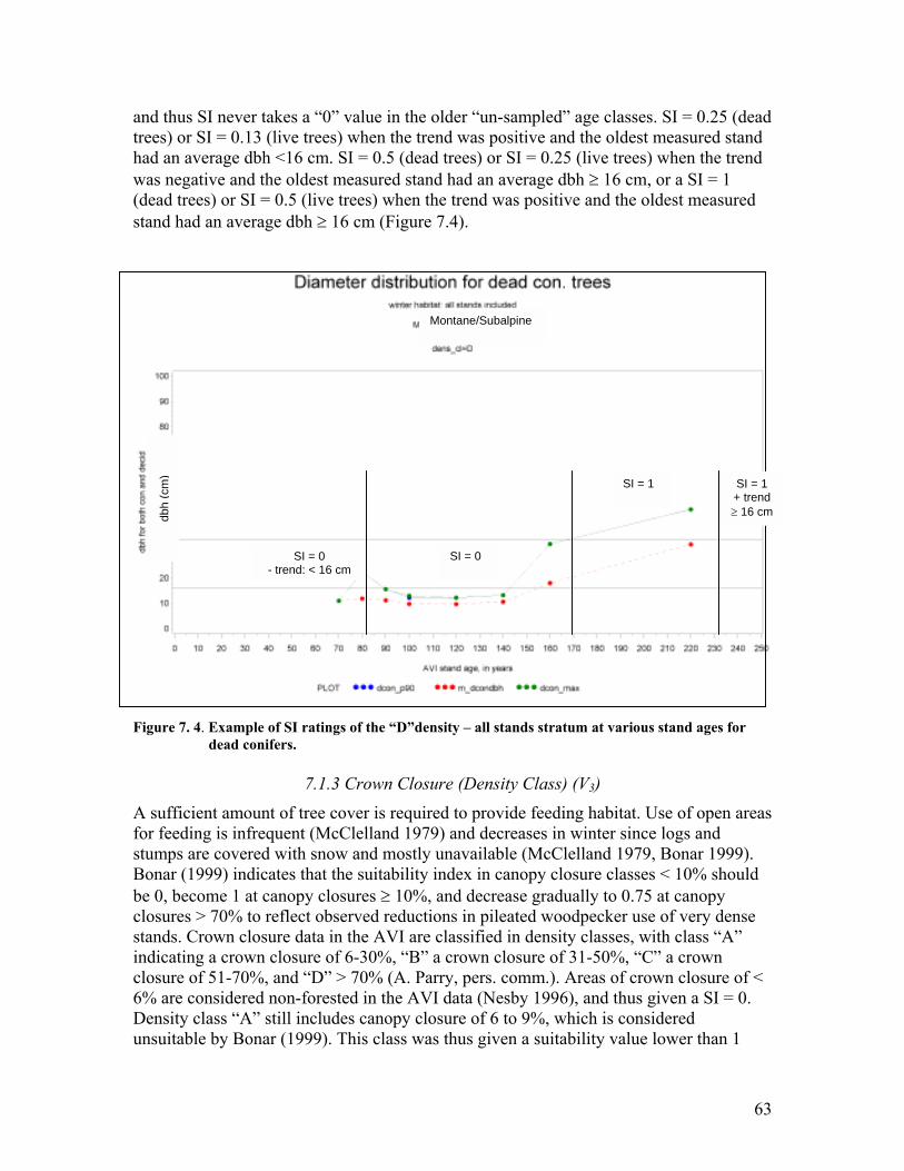
63
and thus SI never takes a �0� value in the older �un-sampled� age classes. SI = 0.25 (dead trees) or SI = 0.13 (live trees) when the trend was positive and the oldest measured stand had an average dbh <16 cm. SI = 0.5 (dead trees) or SI = 0.25 (live trees) when the trend was negative and the oldest measured stand had an average dbh ≥ 16 cm, or a SI = 1 (dead trees) or SI = 0.5 (live trees) when the trend was positive and the oldest measured stand had an average dbh ≥ 16 cm (Figure 7.4).
Figure 7. 4. Example of SI ratings of the �D�density � all stands stratum at various stand ages for
dead conifers.
7.1.3 Crown Closure (Density Class) (V3)
A sufficient amount of tree cover is required to provide feeding habitat. Use of open areas for feeding is infrequent (McClelland 1979) and decreases in winter since logs and stumps are covered with snow and mostly unavailable (McClelland 1979, Bonar 1999). Bonar (1999) indicates that the suitability index in canopy closure classes < 10% should be 0, become 1 at canopy closures ≥ 10%, and decrease gradually to 0.75 at canopy closures > 70% to reflect observed reductions in pileated woodpecker use of very dense stands. Crown closure data in the AVI are classified in density classes, with class �A� indicating a crown closure of 6-30%, �B� a crown closure of 31-50%, �C� a crown closure of 51-70%, and �D� > 70% (A. Parry, pers. comm.). Areas of crown closure of < 6% are considered non-forested in the AVI data (Nesby 1996), and thus given a SI = 0. Density class �A� still includes canopy closure of 6 to 9%, which is considered unsuitable by Bonar (1999). This class was thus given a suitability value lower than 1
dbh
(cm
)
Montane/Subalpine
SI = 0 - trend; < 16 cm
SI = 0
SI = 1 SI = 1 + trend≥ 16 cm

64
(0.9). Classes �B� and �C� were given a suitability value of 1, and class �D� a suitability value of �0.75� (Figure 7.5).
0
0.2
0.4
0.6
0.8
1
A B C D Non-forestedAVI Density Class
Suita
bilit
y In
dex
Figure 7. 5. Habitat suitability index for crown closure (V3) for the pileated woodpecker.
7.1.4 Distance from Suitable Nesting Habitat (V4)
Pileated woodpecker pairs maintain a territory all year round (Bull and Jackson 1995). No territory information was available for the SHARP area, but in west-central Alberta pileated woodpecker territories were 1000 � 4000 ha in size and averaged 2000 ha (Bonar 1999). The model assumes that feeding opportunities are no longer useful if located beyond 3500 m (the radius of a 4000 ha territory) of suitable nesting habitat. Only the stands in which V1 (nesting/ roosting habitat) had a SI ≥ 0.5 were considered in determining distance from suitable nesting habitat. From zero to 2500 m (radius of a 2000 ha circle), V4 was given a SI = 1. As distance further increased toward 3500 m, the suitability of the habitat for feeding gradually decreased to SI= "0" (Figure 7.6).
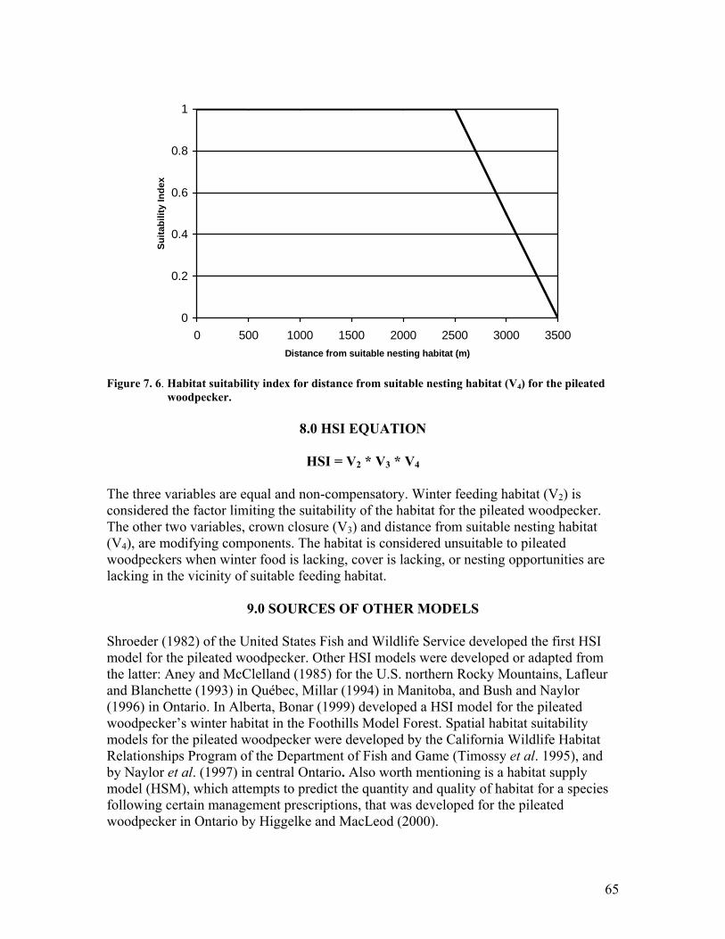
65
0
0.2
0.4
0.6
0.8
1
0 500 1000 1500 2000 2500 3000 3500Distance from suitable nesting habitat (m)
Suita
bilit
y In
dex
Figure 7. 6. Habitat suitability index for distance from suitable nesting habitat (V4) for the pileated
woodpecker.
8.0 HSI EQUATION
HSI = V2 * V3 * V4
The three variables are equal and non-compensatory. Winter feeding habitat (V2) is considered the factor limiting the suitability of the habitat for the pileated woodpecker. The other two variables, crown closure (V3) and distance from suitable nesting habitat (V4), are modifying components. The habitat is considered unsuitable to pileated woodpeckers when winter food is lacking, cover is lacking, or nesting opportunities are lacking in the vicinity of suitable feeding habitat.
9.0 SOURCES OF OTHER MODELS Shroeder (1982) of the United States Fish and Wildlife Service developed the first HSI model for the pileated woodpecker. Other HSI models were developed or adapted from the latter: Aney and McClelland (1985) for the U.S. northern Rocky Mountains, Lafleur and Blanchette (1993) in Québec, Millar (1994) in Manitoba, and Bush and Naylor (1996) in Ontario. In Alberta, Bonar (1999) developed a HSI model for the pileated woodpecker�s winter habitat in the Foothills Model Forest. Spatial habitat suitability models for the pileated woodpecker were developed by the California Wildlife Habitat Relationships Program of the Department of Fish and Game (Timossy et al. 1995), and by Naylor et al. (1997) in central Ontario. Also worth mentioning is a habitat supply model (HSM), which attempts to predict the quantity and quality of habitat for a species following certain management prescriptions, that was developed for the pileated woodpecker in Ontario by Higgelke and MacLeod (2000).

66
10.0 HABITAT SUITABILITY MAP Please refer to map 7.1 for a cartographic representation of potential habitat for the pileated woodpecker within the Southern Headwater at Risk Project area.
11.0 LITERATURE CITED Alberta Natural Heritage Information Centre. 2002. List of all vascular plant elements.
[URL: http://www.cd.gov.ab.ca/preserving/parks/anhic/docs/vascular_plant_list.pdf ]. Accessed [16 October 2003].
Alberta Sustainable Resource Development. 2001. The General Status of Alberta Wild
Species 2000. Alberta Sustainable Resource Development, Fish and Wildlife Service. Pub No I/023. Edmonton, AB. 46 pp.
Aney, W.C. and B.R. McClelland. 1985. Habitat suitability index model for northern
Rocky Mountain pileated woodpeckers. Unpublished Report. Univ. of Montana. 31pp.
Aubry, K.B., and C.M. Raley. 1994. Landscape- and stand-level studies of pileated
woodpeckers: design constraints and stand-level results. Northwest Sci. 68(2):113.
Bonar, R.L. 1999. Pileated woodpecker winter habitat � habitat suitability index model.
Weldwood of Canada Ltd., unpublished document. Hinton, AB. 8 pp. Bonar, R. L. 2000. Availability of pileated woodpecker cavities and use by other species.
J. Wildl. Manage 64: 52-59. Bull, E.L. 1987. Ecology of the Pileated Woodpecker in northeastern Oregon. J. Wildl.
Manage. 51:472-481. Bull, E.L., Holthausen, R.S., and M.G. Henjum. 1992. Roost trees used by pileated
woodpeckers in northeastern Oregon. J. Wildl. Manage 56: 786-793. Bull, E.L, and R.S. Holthausen. 1993. Habitat use and management of pileated
woodpeckers in northeastern Oregon. J. Wildl. Manage 57: 335-345. Bull, E.L., and J.E. Jackson. 1995. Pileated woodpecker (Dryocopus pileatus). In: The
Birds of North America, No. 148 (A. Poole and F. Gill, eds.). The Academy of Natural Sciences, Philadelphia, PA, and The American Ornithologists� Union, Washington, D.C. 24 pp.

67
Bush, P.G., and B.J. Naylor. 1996. A habitat suitability model for the pileated woodpeckers in the Great Lakes � St. Lawrence forest of Ontario. Ontario Ministry of Natural Resources, SCST Technical Report.
Campbell, R.W., Dawe, N.K., Dawe, N.K., McTaggart-Cowan, I., Cooper, J.M. Kaiser,
G.W., and M.C.E. McNall. 1990. The Birds of British Columbia, Volume 2: Non-passerines: Diurnal birds of prey through woodpeckers. Royal British Columbia Museum, Victoria, BC. 636 pp.
Conner, R.N., Miller, O.K.Jr., and C.S. Adkisson. 1976. Woodpecker dependence of trees
infected by fungal heart rots. Wilson Bulletin 88: 575-581. Godfrey, W.E. 1986. The birds of Canada, revised edition. National Museum of Natural
Sciences, National Museums of Canada, Ottawa, ON. 595 pp. Greidanus, G. 2003. C5 woodpecker habitat study: draft November 17, 2003.
Unpublished document, Forest Management Branch, Alberta Sustainable Resource Development. 3 pp. + appendices.
Higgelke, P.E., and H.L. MacLeod. 2000. Pileated woodpecker (Dryocopus pileatus).
Unpublished report prepared for Millar Western Forest Products Biodiversity Assessment Project. 18 pp. [URL: http://giant.lakeheadu.ca/carisweb/hsm/models/pileated_woodpecker_HSM.pdf].
Hoyt, S.F. 1957. The ecology of the pileated woodpecker. Ecology 38: 246-256. Kilham, L. 1979. Courtship and the pair-bond of pileated woodpeckers. The Auk 96:
587-94. Lafleur, P. É. and P. Blanchette. 1993. Développement d'un indice de qualité de l'habitat
pour le Grand Pic (Dryocopus pileatus L) au Québec. Gouvernement du Québec, Ministère du Loisir, de la Chasse et de la Pêche, Direction générale de la ressource faunique, Gestion intégrée des ressources, document technique 93/3. 36 pp. [URL: http://www.fapaq.gouv.qc.ca/fr/etu_rec/exec/iqh/guides/IQH_GRAND_PIC.doc.]
McClelland, B. R. 1979. The pileated woodpecker in forests of the northern Rocky
Mountains. Pp 283-99. In: J. G. Dickson, R. N. Conner, R. R. Fleet, J. A. Jackson and J. C. Kroll (eds). The role of insectivorous birds in forest ecosystems. Academic Press, New York, NY. 381 pp.
Mellen, T. K., E. C. Meslow, and R. W. Mannan. 1992. Summertime home range and
habitat use of pileated woodpeckers in western Oregon. J. Wildl. Manage 56: 96-103.

68
Millar, B.R. 1994. Habitat suitability index model: Pileated Woodpecker (Dryocopus pileatus). Draft report to Manitoba Department of Natural Resources, Wildlife Branch, Winnipeg, MB. 41 pp.
Naylor, B.J., P. Bush, and F. Levec. 1997. Spatial and nonspatial habitat suitability model
for the Pileated Woodpecker in Great Lakes- St. Lawrence forest of central Ontario. Ont. Min. Nat. Res., North Bay, CRST Tech. Rpt. No. 49. 15 pp.
Nesby, R. 1996. Alberta Vegetation Inventory � Standards Manual. Final Draft, Version
2.2. Data Acquisition Branch, Resource Data Division, Alberta Environmental Protection. Unpublished document. 42 pp. + appendices.
Parks, C.G., Bull, E.L., and T.R. Torgersen. 1997. Field guide for the identification of
snags and logs in the interior Columbia River basin. Gen. Tech. Rep. PNW-GTR-390. US. Department of Agriculture, Forest Service. Pacific Northwest Research Station. Portland, OR. 40 pp.
Renken, R. B., and E. P. Wiggers. 1989. Forest characteristics related to pileated
woodpecker territory size in Missouri. Condor 91: 642-652. Salt, W.R., and J.R. Salt. 1976. The birds of Alberta. Hurtig Publishers, Edmonton, AB.
498 pp. Semenchuk, G.P. 1992. Atlas of breeding birds of Alberta. Federation of Alberta
Naturalists, Edmonton, AB. 390 pp. Shroeder, R.L. 1982. Habitat suitability index models: pileated woodpecker. U.S. Dept.
Int., Fish Wildl. Serv. FWS/OBS-82/10.39. 15 pp. Stelfox, J.B. (ed.) 1995. Relationships between stand age, stand structure, and
biodiversity in aspen mixedwood forests in Alberta. Jointly published by Alberta Environmental Centre (AECV95�R1), Vegreville, AB, and Canadian Forest Service (Project No. 0001A), Edmonton, AB. 308 pp.
Timossi, I. C., Woodard, E. L., and R. H. Barrett. 1995. Habitat suitability models for use
with ARC/INFO: pileated woodpecker. Calif. Dept. of Fish and Game, CWHR Program, Sacramento, CA. CWHR Tech. Report No. 16. 26 pp.

69
Map 7. 1. Potential habitat for the pileated woodpecker in the SHARP area.

70
Appendix 7. 1. Relating field-measured stand dbh to the Alberta Vegetation Inventory (AVI) stand origin (modified from Greidanus 2003). Objective:
To provide some basic forest statistics connecting tree level data to a general AVI stratum and age class combination. This will allow us to estimate which AVI types are likely to contain the trees needed by woodpeckers at the landscape level for foraging and nesting. Source data:
Inventory data was taken from the C5, B7 (now B9) and B8 (now B10) FMUs. Only the data from the Montane and Subalpine natural sub-regions were used. Volumes were not used, so the LFD compilation procedures do not need to be described. Three plots were placed within each stand. Each plot was 100 m2, creating a simple expansion factor of 1001. Whether these trees exist, or are uniformly distributed across the landscape, are other issues. A minimum sample diameter of 7-10 cm was used, depending on the cruise. Trees below this diameter were not tallied in the main inventory plot, making it difficult to estimate conditions for young or small-diameter stands. Approach:
Diameters were examined at the landscape level. All dates reference the AVI stand age. Stand age was calculated by subtracting the AVI origin from the sample date, then rounded down to the nearest 10-year increment.
Prior to examining the diameters, plot data was pooled by age class and strata for two broad habitat types. The more-detailed breeding habitat used the following strata:
• Pine leading: Stands with 80% conifer in the overstorey, with pine as the dominant conifer species.
• Spruce leading: Stands with 80% conifer in the overstorey, with White Spruce or Balsam Fir as the dominant conifer species.
• Douglas-fir present: Stands with 80% conifer in the overstorey, with Fd (Douglas-fir) present in either the SP1 or SP2 column of the AVI label. This may include both pure stands, and Pl/Fd (lodgepole pine/Douglas-fir) stands.
• Se/Fa/La: Stands with 80% conifer in the AVI label, with a high-elevation conifer species present2.
• Mixed-woods: Stands with less than 80% but more than 20% conifer in the AVI label. Normally these are broken into conifer-leading and deciduous-leading, but were joined into one strata due to data limitations.
• Deciduous leading: Stands with 20% or less conifer in the AVI label. The remaining percentage is deciduous, by crown closure.
Only stands that had an AVI height of 12m or taller were allowed to contribute to the breeding habitat. The less-detailed winter habitat collapsed the above strata into one
1 For example, each tree sampled in the plot would represent 100 theoretical trees per ha on the landscape. 2 Se=Engelmann spruce, Fa=Alpine Fir, La=Alpine larch.

71
broad landscape stratum, and examined only the conifer / deciduous differences. All heights contributed to the winter habitat.
In addition to species composition, three density classes were used. The AVI labels were used to group the data into �A�, �B+C� and �D� density classes.
Five broad species types were examined within each of these strata. The diameters for live conifer, live deciduous and live Douglas-fir, dead conifer and dead deciduous were examined. Further species-information could not be pulled out for the dead trees, but it might be a reasonable assumption that they could be tied to the overstorey label.
So, as an example, all the trees sampled in the 110-year old B+C density pine leading plots were pooled. Statistics were calculated on this discrete pool, and plotted. Since a best-fit relationship was not developed, a rather �jagged� looking relation was often the result. Three statistics were used. The maximum and average diameters, as well as the diameter at the 90th percentile (P90), were all calculated. The last was used to explore the range of diameters at the high-end. A stratum with few large trees will have a similar max and P90 value, while a stratum with more large trees should have more of a gap. Minimum diameters were not examined because of the minimum sample size of 7-10 cm. When plotting diameters for live trees, a minimum of three trees was needed to contribute to the age-class average. These three trees were specific to the strata, and were intended to improve the accuracy of the resulting statistic. For example, 3 deciduous trees by age class in the deciduous strata, or 3 Douglas-fir trees in the Douglas-fir strata. This rule was relaxed for dead trees, where only a single tree had to be present by age class.
While this approach does give you the benefit of finding the general trend on the landscape without having to model a best-fit relationship, it does not let you make assumptions about typical stand conditions. The stand-level variation is lost, which may affect how effective the model is finding appropriate stands that are suitable for woodpeckers. The geographic attributes are also lost, as the data is pooled at the landscape level. The high-diameter stands may all be spatially connected, but this won�t be found in this model. Results: A graphics dump was done through SAS, and exported as .png files. These files were sent to F.Blouin for further processing.

72
Figure 7. 7. Sample graph for the A-denstiy Fd-leading stratum for the breeding habitat. There is a general trend for the diameter of the dead conifer trees to increase as the stand ages. For stratum with a small number of samples, the P90 tends to be the same value as the maximum, and is plotted underneath its symbol.
Inferences about the age when the habitat becomes suitable for woodpeckers will have to be made on the basis of professional opinion.
dbh
(cm
) Montane/Subalpine
73
Clark�s Nutcracker (Nucifraga columbiana)
François Blouin Wildlife Consultant, Lethbridge, AB
1.0 PURPOSE AND LIMITATIONS
The purpose of this model is to indicate potential spring to fall habitat for the Clark�s nutcracker (Nucifraga columbiana) within the Southern Headwaters at Risk Project (SHARP) area. Also, as it is a landscape level model with coarse variables, it may not be directly applicable to other areas or for site-specific analysis. This model is based on published and unpublished literature and expert opinion, and has not been field-tested.
2.0 GENERAL INFORMATION The Clark�s nutcracker is a jay-sized corvid, light to medium grey in colour, with white rectrices on glossy black tail and white patches on glossy black wings, long and pointed heavy black bill, and a shorter tail than that of the similar-looking gray jay (Semenchuk 1992, Tomback 1998). It has a unique sublingual pouch that expands for seed transportation (Tomback 1998). It is usually noisy and makes a harsh grating call like �char-r-r� or �kra-a-a� repeated two or three times (Godfrey 1986). It ranges from the eastern slopes of the Coast Ranges in southern British Columbia east to the eastern slopes of the Rocky Mountains in southern Alberta, south through the mountains, the Great Basin ranges, the Nevada ranges, the California mountains, down to northwestern New Mexico (Tomback 1998). The Clark�s nutcracker is a year-round resident of Alberta and is found predominantly in the Rocky Mountain Natural Region (Achuff 1994), from the montane landscape up to the tree line (Semenchuk 1992). Records exist in the adjacent Foothills region and sporadic irruptions have brought birds as far east as the Cypress Hills (Salt and Salt 1976, Semenchuk 1992). Despite being a pine seed specialist (85% - 95% of its diet), it is also an opportunistic forager, feeding on insects, spiders, small mammals, eggs, nestlings, carrion, human scraps, berries, and buds (Semenchuk 1992, Campbell et al. 1997, Tomback 1998). The Clark�s nutcracker has a mutualistic relationship with whitebark pine (Pinus albicaulis), limber pine (Pinus flexilis), and other large-seeded pine species in other areas of its range (Tomback 1998). The Clark�s nutcracker relies heavily on the harvesting and �caching� of wingless seeds from those pine species in its annual cycle, and in turn, those pines depend on it for seed dispersal as well as recolonisation after disturbance (Lanner 1980, Tomback and Linhart 1990, Vander Wall 1990, Tomback 1998, Webster and Johnson 2000). In fact, the range of the Clark�s nutcracker corresponds well with that of those pines in U.S. and Canada (Tomback 1998). There are currently serious concerns about the limber and whitebark pines in western Canada and United States as five-needle pines are being threatened by the synergistic effect of changes in composition of successional coniferous forest from years of fire suppression, the introduced white pine blister rust (Cronartium ribicola), and mountain pine beetle epidemics (Peterson 1999, Tomback 2003). In addition, Clark�s nutcracker belongs to the

74
Corvidae family, which has recently been affected by the West Nile Virus (Health Canada 2003), causing a concern for this species as the virus makes its way westward (R. Quinlan, pers. comm.). Currently, Clark�s nutcracker is considered �secure� in Alberta (Alberta Sustainable Resource Development 2001).
3.0 GENERAL HABITAT ASSOCIATIONS The Clark�s nutcracker typically inhabits open or semi-open coniferous forests, clearings, edges, and burns at higher elevations, migrating into valleys for winter (Godfrey 1986, Semenchuk 1992). It prefers forests dominated by large seeded pines such as whitebark pine, ponderosa pine (Pinus ponderosa), and limber pine from which it derives its main diet of seeds (Tomback 1998). Breeding habitat includes coniferous forest from montane to subalpine zones. In the fall and winter, and during years of conifer seed-crop failure, it also uses anthropogenic habitats such as campgrounds, picnic grounds, ski resorts, garbage dumps, agricultural fields, and residential areas where bird feeders occur (Campbell et al. 1997).
3.1 Breeding Habitat In Alberta, the Clark�s nutcracker generally begins nesting in March (Semenchuk 1992). It predominantly breeds in the coniferous forests of the subalpine region, with one population known to breed around the town of Banff in the Montane Natural Subregion (Achuff 1994). Little is known about the specific breeding habitat requirements of the Clark�s nutcracker in the province. In British Columbia, breeding normally occurs at high elevations in open to semi-open subalpine coniferous forests, in mixed Douglas-fir � ponderosa pine forests on the lower mountain slopes, and in ponderosa pine parklands of the benchlands. Most nests at lower elevations were found on steep slopes in ponderosa pine and Douglas-fir, and at higher elevations in whitebark pine, alpine larch (Larix lyallii), and spruce (Picea spp; Campbell et al. 1997). Clark�s nutcracker may prefer nesting in small stands of forest trees near forest edge or above valleys, with some shelter from the wind. Nest trees are sometimes on south-facing slope or in canyon bottoms (Tomback 1998).

75
3.2 Summer Habitat In late spring, in high mountains, fledglings and most breeders and non-breeders move up-slope to subalpine elevations, especially where whitebark and/or limber pine occur (Tomback 1998). They follow the receding snowline to uncover caches, reaching alpine storage areas by July (Campbell et al. 1997). Depending on the seed crop production, they may remain at high elevations until October or November, although some birds move down to lower elevation seed sources by late September. In the U.S., preferred higher elevations habitats include open to semi-open steep rocky slopes or small hills or ridges interspersed with moist meadows, small lakes, and creeks, and dominated by stands of shrubby whitebark or limber pine, sometimes mixed with fir, spruce or other pines (Tomback 1998). When seedcrop is poor, individuals move down into the montane coniferous forest in August (Tomback 1998).
3.3 Fall and Winter Habitat In the subalpine areas, in the autumn months, Clark�s nutcrackers harvest pine seeds and cache them at variable distances away in open areas or places of low snow accumulation and early snowmelt (Campbell et al. 1997). In higher mountain regions, most nutcrackers descend to lower elevations from late September through November into Douglas-fir, limber pine and ponderosa pine communities (Tomback 1998). They overwinter at lower elevations and may wander widely, sometimes more than 100 km (Tomback 1998). Habitats such as ski resorts where birds find human scraps, and residential areas where bird feeders occur are also used (Semenchuk 1992, Campbell et al. 1997). On the mountain slopes, the nutcracker supplements its winter diet of conifer seeds by searching big-game ranges and scavenging on carcasses (Campbell et al. 1997).
4.0 SPECIAL HABITAT ASSOCIATIONS Both the winter and the summer ranges of the Clark�s nutcracker in Canada are tightly linked to distribution of the large seeded pines (Campbell et al. 1997, Tomback 1998). In Alberta and the SHARP area, these include the whitebark pine and the limber pine.
5.0 HABITAT AREA REQUIREMENTS Little information is available about habitat area requirements for the Clark�s nutcracker. One nesting territory in Missoula, MT, was estimated at 0.85 ha (2.1 acres; Mewaldt 1956). Family groups and nonbreeding individuals have been observed occupying home range of about 200 ha in spring and summer, and unless cone crops fail, overwintering birds occupy a home range as well (unspecified size; Tomback 1998). These home ranges are likely based on location of seed stores (Tomback 1998). With good seed production, nutcrackers stayed within an area of about 15,000 ha including seasonal movements (Tomback 1998). Long-distance dispersal is constrained by the need to remain in proximity of food stores.

76
6.0 ASSOCIATED SPECIES In Montana, species recorded in the same habitat as the Clark�s nutcracker and that occur in Alberta include Steller's jay (Cyanocitta stelleri), black-billed magpie (Pica hudsonia), black-capped chickadee (Poecile atricapilla), mountain chickadee (Poecile gambeli), white-breasted nuthatch (Sitta carolinensis), red-breasted nuthatch (Sitta canadensis), American robin (Turdus migratorius), mountain bluebird (Sialia currucoides), golden-crowned kinglet (Regulus satrapa), Cassin�s finch (Carpodacus cassinii), red crossbill (Loxia curvirostra), dark-eyed junco (Junco hyemalis), hairy woodpecker (Picoides villosus), northern flicker (Colaptes auratus), northern pygmy-owl (Glaucidium gnoma), and red-tailed hawk (Buteo jamaicensis) (Mewaldt 1956). Other species recorded with Clark�s nutcrackers in the Sierra Nevada and that also occur in Alberta include pine grosbeak (Pinicola enucleator), golden-mantled ground squirrel (Spermophilus lateralis), chipmunks, squirrels (Tamiasciurus spp), Cooper�s hawk (Accipiter cooperii), Prairie Falcon (Falco mexicanus), and northern goshawk (Accipiter gentilis) (Tomback 1978). Other species of the same area reported mobbed by Clark�s nutcracker include red-tailed hawk, Cooper�s hawk, Swainson hawk (Buteo swainsoni), golden eagle (Aquila chrysaetos), and great horned owl (Bubo virginianus) (Tomback 1998). American kestrel (Falco sparverius) and sharp-shinned hawks (Accipiter striatus) are mentioned as small predators that are provoked and chased by the nutcracker for play, and northern shrikes (Lanius excubitor) also occur within the range of the nutcracker in winter (Tomback 1998). Semenchuk (1992) adds that nutcrackers compete with gray jays (Perisoreus canadensis) in Alberta for human scraps.
7.0 THE HSI MODEL
7.1 Selected Habitat Variables
7.1.1 Tree Species (V1)
There is very limited habitat information specific to Alberta in the literature. However, the presence of large-seeded pines such as whitebark pine and limber pine appears to be a very important factor controlling Clark�s nutcrackers distribution in Canada in all seasons (Tomback 1998). Other conifer seeds including Douglas-fir are also taken but to a much lesser extent (Tomback 1998). Campbell et al. (1997) indicated that whitebark and limber pine have been found to comprise between 85% and 95% of nutcrackers� diet. In addition, Douglas-fir was used in 33% of the nests found in the Okanagan valley (Campbell et al. 1997). The tree species categorical variable (V1) drawn from the Alberta Vegetation Inventory (AVI; Nesby 1996) was thus assigned a suitability index value of �1� wherever whitebark pine or limber pine occurred, 0.33 where Douglas-fir occurred, �0.1� (or 1 - 0.9) where any other conifer species occurred, and �0� where the other tree species were found (Figure 8.1).

77
0
0.2
0.4
0.6
0.8
1
Limber Whitebark Douglas-fir Other Conifers Other spp.
Tree Species
Suita
bilit
y In
dex
Figure 8. 1. Habitat suitability index for tree species (V1) for the Clark�s nutcracker.
7.1.2 Crown Closure (Density Class) (V2)
The Clark�s nutcracker breeds and spends its summer in open to semi-open coniferous forests or subalpine forests (Campbell et al. 1997; Tomback 1998). No specific information is available about the �degree of openness� of the habitat required by this species, but open areas are needed for seed storage or recovery (Campbell et al. 1997). Habitat openness was estimated using the categorical variable �crown closure� of the AVI (Nesby 1996). A crown closure of 6% - 50% representing open and semi-open habitats (density classes A and B) was given a suitability index of �1�. Crown closure of 51%-70% (density class C) still exhibits between 30% and 49% openness and thus was given a suitability index value of 0.5; while crown closure > 70% may not be as suitable but birds could still use the seed from the area and move them to other locations, up to a few kilometres (Campbell et al. 1997, Tomback 1998). It was thus given a suitability index value of �0.25� (Figure 8.2). Areas of crown closure of < 6% are not considered forested in the AVI (Nesby 1996) but were given a suitability index value of �0.1� because there could be isolated seed-producing trees for food and open areas for seed caching.
0
0.2
0.4
0.6
0.8
1
A B C D OtherCrown Closure Category
Suita
bilit
y In
dex
Figure 8. 2. Habitat suitability index for crown closure (V2) for the Clark�s nutcracker.
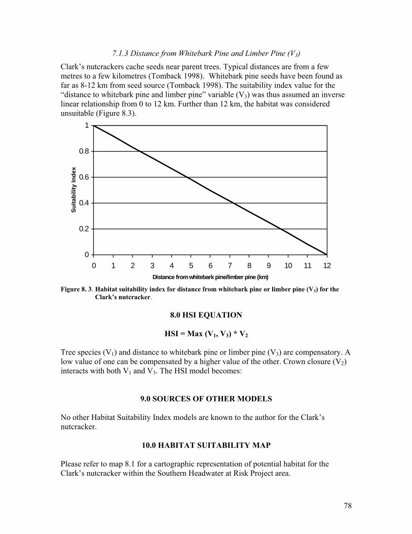
78
7.1.3 Distance from Whitebark Pine and Limber Pine (V3)
Clark�s nutcrackers cache seeds near parent trees. Typical distances are from a few metres to a few kilometres (Tomback 1998). Whitebark pine seeds have been found as far as 8-12 km from seed source (Tomback 1998). The suitability index value for the �distance to whitebark pine and limber pine� variable (V3) was thus assumed an inverse linear relationship from 0 to 12 km. Further than 12 km, the habitat was considered unsuitable (Figure 8.3).
0
0.2
0.4
0.6
0.8
1
0 1 2 3 4 5 6 7 8 9 10 11 12Distance from whitebark pine/limber pine (km)
Suita
bilit
y In
dex
Figure 8. 3. Habitat suitability index for distance from whitebark pine or limber pine (V3) for the
Clark�s nutcracker.
8.0 HSI EQUATION
HSI = Max (V1, V3) * V2 Tree species (V1) and distance to whitebark pine or limber pine (V3) are compensatory. A low value of one can be compensated by a higher value of the other. Crown closure (V2) interacts with both V1 and V3. The HSI model becomes:
9.0 SOURCES OF OTHER MODELS No other Habitat Suitability Index models are known to the author for the Clark�s nutcracker.
10.0 HABITAT SUITABILITY MAP Please refer to map 8.1 for a cartographic representation of potential habitat for the Clark�s nutcracker within the Southern Headwater at Risk Project area.

79
11.0 LITERATURE CITED Achuff, P.L. 1994. Natural regions, subregions and natural history themes of Alberta: A
classification for protected areas management. Report No.2. Prepared for Parks Services and Natural and Protected Areas, Alberta Government. 72 pp.
Alberta Sustainable Resource Development. 2001. The General Status of Alberta Wild
Species 2000. Alberta Sustainable Resource Development, Fish and Wildlife Service. Pub No I/023. Edmonton, AB. 46 pp.
Campbell, R.W., Dawe, N.K., McTaggart-Cowan, I., Cooper, J.M. Kaiser, G.W.,
McNall, M.C.E., and G.E.J. Smith.1997. The Birds of British Columbia, Volume 3: Passerines: Flycatchers through Vireos. UBC Press, Vancouver, BC. 696 pp.
Godfrey, W.E. 1986. The birds of Canada, revised edition. National Museum of Natural
Sciences, National Museums of Canada, Ottawa, ON. 595 pp. Health Canada. 2003. West Nile virus. URL: http://www.hc-
sc.gc.ca/english/westnile/index.html. [Accessed 9 October 2003]. Lanner, R.M. 1980. Avian seed dispersal as a factor in the ecology and evolution of
limber and whitebark pines. In: Proceedings Sixth North American Forest Biology Workshop, Univ. Alberta, Edmonton, AB. 48 pp.
Lanner, R.M., and S.B. Vander Wall. 1980. Dispersal of limber pine seed by Clark�s
nutcracker. J. Forestry 78: 637-639. Mewaldt, L.R. 1956. Nesting behavior of the Clark nutcracker. Condor. 58: 3-23. Nesby, R. 1996. Alberta Vegetation Inventory � Standards Manual. Final Draft, Version
2.2. Data Acquisition Branch, Resource Data Division, Alberta Environmental Protection. Unpublished document. 42 pp. + appendices.
Peterson, K.T. 1999. Whitebark pine (Pinus albicaulus) decline and restoration in Glacier
National Park. M.Sc Thesis, University of North Dakota, Grand Forks, ND. 75 pp.
Salt, W.R., and J.R. Salt. 1976. The birds of Alberta. Hurtig Publishers, Edmonton, AB.
498 pp. Semenchuk, G.P. 1992. Atlas of breeding birds of Alberta. Federation of Alberta
Naturalists, Edmonton, AB. 390 pp. Tomback, D.F. 1978. Foraging strategies of Clark�s nutcracker. Living Bird 16: 123-161.
80
Tomback, D.F. 1998. Clark�s nutcracker (Nucifraga columbiana). In: The Birds of North America, No. 331 (A. Poole and F. Gill, eds.). The Academy of Natural Sciences, Philadelphia, PA, and The American Ornithologists� Union, Washington, DC, 24 pp.
Tomback, D.F. 2003. Whitebark pine: status, trends, strategies in the U.S.A. In: Parks
Canada (ed). Whitebark and Limber Pine Workshop-Workshop Proceedings, February 18th and 19th, 2003. Calgary, AB. 39 pp.
Tomback, D.F., and Y.B. Linhart. 1990. The evolution of bird-dispersed pines. Evol.
Ecol. 4: 185-219. Vander Wall, S.B. 1990. Food hoarding in animals. Univ. of Chicago Press, Chicago, IL.
445 pp. Webster, K.L., and E. A. Johnson. 2000. The importance of regional dynamics in local
populations of limber pine (Pinus flexilis). Ecoscience 7(2): 175-182.

81
Map 8. 1. Potential habitat for the Clark�s nutcracker in the SHARP area.

82
Sprague�s Pipit (Anthus spragueii)
Julie P. Landry Alberta Conservation Association, Lethbridge, AB
1.0 PURPOSE AND LIMITATIONS The purpose of this model is to indicate potential nesting and foraging habitat for Sprague�s pipit (Anthus spragueii) within the Southern Headwaters At Risk Project (SHARP) area. As this is a landscape level model with coarse variables, it may not be directly applicable to other areas or for site-specific analysis. This model is based on published and unpublished literature and expert opinion, and has not been field-tested.
2.0 GENERAL DESCRIPTION The Sprague�s pipit is a songbird of the native grasslands (Sibley 2000), similar in appearance to sparrows such as the vesper sparrow (Pooecetes gramineus) and the Baird�s sparrow (Ammodramus bairdii) (Salt and Wilk 1958). Distinguishing features include buff and streaked upper feathers (Semenchuk 1992), extensive white on its outer tail feathers (Sibley 2000), and a slender pointed beak (Salt and Wilk 1958). The Sprague�s pipit has a distinctive song, which is sung from a high altitude and is a �rolling, jingling cascade of high, dry whistles� (Sibley 2000). Breeding occurs in southern Alberta, Saskatchewan, Manitoba, Minnesota, North Dakota, and Montana (Sibley 2000). This species migrates to wintering grounds in the southern United States and Mexico (Salt and Wilk 1958). In Alberta, The General Status of Alberta Wild Species 2000 (Alberta Sustainable Resource Development 2001) designates the Sprague�s pipit as a �Sensitive� species, while the Committee on the Status of Endangered Wildlife in Canada (COSEWIC 2001) has the Sprague�s pipit classified as �Threatened.�
3.0 HABITAT ASSOCIATIONS
3.1 Food The Sprague�s pipit is predominantly insectivorous, catching prey on or near the ground (Semenchuk 1992, Salt and Wilk 1958). In May, beetles comprise more than 40% of the adult diet and in September grasshoppers comprise 91% (Maher 1974, as cited in Prescott 1997). The nestling diet consists primarily of grasshoppers, but also may include lepidopteran larvae, leaf hoppers, spiders, and ants (Harris 1933, as cited in Prescott 1997).

83
3.2 Cover The Sprague�s pipit tends to occupy native grassland habitats (Wilson and Belcher 1989, Dale et al. 1997) containing very little or no woody vegetation (Davis and Duncan 1999, Dale 1983, as cited in Prescott 1997), with non-native areas populated to a significantly lower extent (Davis and Duncan 1999). Research on these birds has shown them occupying grassland habitats with varying characteristics. Sutter et al. (1996) described that this bird forages in dense grassy vegetation, whereas, Sutter and Brigham (1998) identified occupied areas as sparse to intermediate in density with intermediate vegetation heights. In Saskatchewan, Sprague�s pipits avoided heavily grazed areas and were positively associated with narrow-leafed grasses equal to or less than 10 cm tall, and were negatively associated with shrubs 20-100 cm tall (Anstey et al. 1995, as cited in Dechant et al. 2001). In North Dakota, if vegetation reached 8cm tall, Sprague�s pipit incidence decreased by 50%, and decreased to less than 5% at vegetation heights of 19 cm (Madden et al. 2000). In addition, Sprague�s pipits were completely absent from areas of deep litter (Sutter 1997) or dense nesting cover (Prescott and Murphy 1999) and from areas that had not seen fire disturbance for >80 years (Madden et al. 1999). In Alberta, Owens and Myres (1973) found that Sprague�s pipit were common on idle native prairie, and to a lesser extent were also found on lightly grazed native prairie with dense grasses. Sprague�s pipits may also occasionally occupy grasslands that receive periodic disturbances such as fire, heavy grazing, and mowing (Owens and Myres 1973). In Alberta, Prescott and Murphy (1996) found that preferred areas had moderate cover diversity and moderate grass height and height variation.
3.3 Nesting Cover Sprague�s pipits build their nests on the ground in small depressions (McConnell et al. 1993) where grass is denser and taller, and where forb and shrub density is low (Sutter 1997). The nests are woven cups lined with coarse and fine graminoids (McConnell et al. 1993) and often have overarched grasses (Salt and Wilk 1958). In Saskatchewan, Sutter (1997) found nest sites had higher grass and sedge cover, lower forb and shrub cover, higher maximum vegetation height, lower bare ground cover, and lower forb density than found at random sites (Table 9.1).
Table 9. 1. Characteristics of nest sites (n=47) in Saskatchewan (Sutter 1997).
Grass and Sedge Cover: 52.7 % Forb and Shrub Cover: 10.5 % Litter Cover: 15.2 % Bare Ground Cover: 16.8 % Maximum Height: 27.7 cm Litter Depth: 2.4 cm

84
4.0 HABITAT AREA REQUIREMENTS Predominantly, Sprague�s pipits have been recorded on larger tracts of native prairie (Owens and Myres 1973). For example, in Saskatchewan the minimum area required was 190 ha (Saskatchewan Wetland Conservation Corporation 1997, as cited in Dechant et al. 2001). Kantrud (1981) found the amount of grazing an area received as well as land usage type depicted how many pairs may occupy an area. It is interesting to note that in Manitoba, brown-headed cowbird brood parasitism was higher on smaller tracts of land (22 ha) than on larger ones (64 ha) (Davis and Sealy 2000, as cited in Dechant et al. 2001).
5.0 ASSOCIATED SPECIES A few species associated with the Sprague�s pipit include the Baird�s sparrow (Ammodramus bairdii), grasshopper sparrow (Ammodramus savannarum), Le Conte�s sparrow (Ammodramus leconteii), western meadowlark (Sturnella neglecta) (Madden et al. 1999), and chestnut-collared longspur (Calcarius ornatus) (Davis and Duncan 1999).
6.0 THE HSI MODEL
6.1 Assumptions and Limitations It will be assumed that all water requirements are attained through consumption of insects because no water requirements have been documented for this species. Since vegetation height, density, and grass to forb ratio could not be determined for this model, it will be assumed that within native grasslands the variability needed for foraging and nesting will be available. Within each quarter section, the native prairie coverage cannot determine if the percent of native grass is contiguous or not. Upon ground truthing, highly suitable areas may not be as suitable as once determined. For our purposes, we will assume native grass is contiguous within each quarter section.
6.2 Selected Habitat Variables
6.2.1 Percent Native Grass (V1)
In Alberta, Prescott and Wagner (1996) observed that Sprague�s pipit were 15 times more common on native fescue or mixed-grass prairie than in tame pastures or agricultural fields. For this model, areas comprised of 25% or more native grass were assigned a suitability value of 1. Since non-native areas are not completely devoid of Sprague�s pipits, zero percent native grass areas did not receive a habitat suitability value of zero but received a low suitability of 0.1. As native grassland percent cover increases from zero, the suitability increases (Figure 9.1).
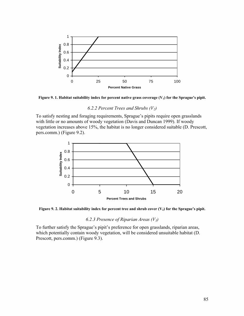
85
0
0.2
0.4
0.6
0.8
1
0 25 50 75 100Percent Native Grass
Suita
bilit
y In
dex
Figure 9. 1. Habitat suitability index for percent native grass coverage (V1) for the Sprague�s pipit.
6.2.2 Percent Trees and Shrubs (V2)
To satisfy nesting and foraging requirements, Sprague�s pipits require open grasslands with little or no amounts of woody vegetation (Davis and Duncan 1999). If woody vegetation increases above 15%, the habitat is no longer considered suitable (D. Prescott, pers.comm.) (Figure 9.2).
0
0.2
0.4
0.6
0.8
1
0 5 10 15 20Percent Trees and Shrubs
Suita
bilit
y In
dex
Figure 9. 2. Habitat suitability index for percent tree and shrub cover (V2) for the Sprague�s pipit.
6.2.3 Presence of Riparian Areas (V3)
To further satisfy the Sprague�s pipit�s preference for open grasslands, riparian areas, which potentially contain woody vegetation, will be considered unsuitable habitat (D. Prescott, pers.comm.) (Figure 9.3).

86
0
0.2
0.4
0.6
0.8
1
Absent PresentPresence of Riparian Areas
Suita
bilit
y In
dex
Figure 9. 3. Habitat suitability index for riparian areas (V3) for the Sprague�s pipit.
7.0 HSI EQUATION
HSI = (V1 * V2 * V3)
The equation used for evaluating nesting and foraging habitat for Sprague�s pipits considers the 3 variables to be equal and non-compensatory. A low value in one of the variables cannot be compensated by a higher value in another. This equation describes a full interaction between the 3 variables, indicating that the use of native grasses as reproductive habitat only occurs where shrub and tree cover is low or nil.
7.1 Other Variables Considered
7.1.1 Grass Height
There was no available database containing information on grass heights. This variable would have been useful in selecting more specific nesting areas for Sprague�s pipits (Sutter 1997).
8.0 SOURCES OF OTHER MODELS One other habitat suitability model for the Sprague�s pipit was created for the M.D. of Foothills No. 31 (Kienzle and Landry 2002).
9.0 HABITAT SUITABILITY MAP Please refer to map 9.1 for a cartographic representation of the potential breeding, nesting, and foraging habitat for the Sprague�s pipit within the SHARP area. This map was produced with the three habitat variables used in the HSI equation: percent native grass, percent trees and shrubs, and presence of riparian areas. Four different suitability ratings, ranging from �highly suitable� to �least suitable,� were categorized on the

87
landscape. If additional information regarding microhabitat for the Sprague�s pipit (e.g. grass height and density) were acquired, highly suitable habitat areas could be more refined.
10.0 LITERATURE CITED Alberta Sustainable Resource Development. 2001. The General Status of Alberta Wild
Species 2000. Alberta Sustainable Resource Development, Fish and Wildlife Service, Publ. No.I/023. Edmonton, AB. 46 pp.
Anstey, D.A., S.K. Davis, D.C. Duncan, and M. Skeel. 1995. Distribution and habitat
requirements of eight grassland songbird species in southern Saskatchewan. Saskatchewan Wetland Conservation Corporation, Regina, Saskatchewan. 11 pp.
COSEWIC. 2001. Canadian species at risk, November 2001. Committee on the Status of
Endangered Wildlife in Canada. 32 pp. Dale, B.C. 1983. Habitat relationships of seven species of passerine birds at Last
Mountain Lake, Saskatchewan. Unpubl. M.Sc. thesis, Univ. Regina, Regina, SK. 119 pp.
Dale, B.C., P.A., Martin, and P.S. Taylor. 1997. Effects of hay management on grassland
songbirds in Saskatchewan. Wildlife Society Bulletin 25(3): 616-626. Davis, S.K. and D.C. Duncan. 1999. Grassland songbird occurrence in native and crested
wheatgrass pastures of southern Saskatchewan. Studies in Avian Biology 19: 211-218.
Davis, S.K., and S.G. Sealy. 2000. Cowbird parasitism and nest predation in fragmented
grasslands of southwestern Manitoba. Pp. 220-228 IN: J. N. M. Smith, T. L. Cook, S. I. Rothstein, S. K. Robinson, and S. G. Sealy, editors. Ecology and management of cowbirds and their hosts. University of Texas Press, Austin, Texas.
Dechant, J.A., M.L. Sondreal, D.H. Johnson, L.D. Igl, C.M. Goldade, M.P. Nenneman,
and B.R. Euliss. 2001. Effects of management on grassland birds: Sprague�s pipit. Northern Prairie Wildlife Research Center, Jamestown, ND. Jamestown, ND, Northern Prairie Wildlife Research Center, Home Page. http://www.npwrc.usgs.gov/resource/literatr/grasbird/pipit/pipit.htm
Harris, R.D. 1933. Observations on a nest of Sprague�s pipit (Anthus spragueii).
Canadian Field Naturalist 47: 91-95. Kantrud, H.A. 1981. Grazing intensity effects of the breeding avifauna of North Dakota
native grasslands. Canadian Field Naturalist 95(4): 404-417.
88
Kienzle, S.T. and J.Landry. 2002. Bird habitat modelling in the municipal district of Foothills No. 31. Unpublished Report. Department of Geography, University of Lethbridge for the M.D. Foothills No.31. 54 pp.
Madden, E.M., A.J. Hansen, and R.K. Murphy. 1999. Influence of prescribed fire history
on habitat and abundance of passerine birds in northern mixed-grass prairie. Canadian Field Naturalist 113(4): 627-640.
Madden, E.M., R.K. Murphy, A.J. Hansen, and L. Murray. 2000. Models for guiding
management of prairie bird habitat in Northwestern North Dakota. American Midland Naturalist 144: 377-392.
Maher, W. J. 1974. Matador project. Birds: III. Food habits. Canadian Committee for the
International Biological Programme Tech. Rept. No. 52, Saskatoon, SK. 107 pp. McConnell, S.D., D.R. Vandendriessche, T.D. Hooper, G.L. Roberts, and A. Roberts.
1993. First occurrence and breeding of Sprague�s pipit, Anthus spragueii, for British Columbia. Canadian Field Naturalist 107: 222-223.
Owens, R.A., and M.T. Myres. 1973. Effects of agriculture upon populations of native
passerine birds of an Alberta fescue grassland. Canadian Journal of Zoology 51: 697-713.
Prescott, D.R.C. 1997. Status of the Sprague�s pipit (Anthus spragueii) in Alberta.
Alberta Environmental Protection, Wildlife Management Division, Wildlife Status Report No. 10, Edmonton, AB. 14 pp.
Prescott, D.R.C., and A.J. Murphy. 1996. Habitat associations of grassland birds on
native and tame pastures of the aspen parkland in Alberta. NAWMP-02. Alberta NAWMP Centre, Edmonton, Alberta. 36 pp.
Prescott, D.R.C., and A.J. Murphy. 1999. Bird populations of seeded grasslands in the
aspen parkland of Alberta. Studies in Avian Biology 19: 203-210. Prescott, D.R.C., and G.M. Wagner. 1996. Avian responses to implementation of a
complementary/rotational grazing system by the North American Waterfowl Management Plan in southern Alberta: the Medicine Wheel project. Alberta NAWMP Centre. NAWMP-018. Edmonton, AB. 24 pp.
Salt, W.R. and A.L. Wilk. 1958. The Birds of Alberta. Lithographed by Hamly Press
Ltd., Edmonton, AB. 511 pp. Saskatchewan Wetland Conservation Corporation (SWCC). 1997. Grassland bird
conservation through Saskatchewan�s native prairie stewardship program. Saskatchewan Wetland Conservation Corporation, Regina, Saskatchewan.

89
Semenchuk, G. P. 1992. The Atlas of breeding birds of Alberta. Federation of Alberta Naturalists, Edmonton, Alberta.
Sibley, D.A. 2000. National Audubon Society. The Sibley Guide to Birds. Alfred A
Knopf, Inc., New York. 545 pp. Sutter, G.C. 1997. Nest-site selection and nest-entrance orientation in Sprague�s pipit.
Wilson Bulletin 109(3): 462-469. Sutter, G.C., and R.M. Brigham. 1998. Avifaunal and habitat changes resulting from
conversion of native prairie to crested wheat grass: patterns at songbird community and species levels. Canadian. Journal of Zoology 76: 869-875.
Sutter, G.C., D.J. Sawatzky, D.M. Cooper, and R.M. Brigham. 1996. Re-nesting intervals
in Sprague�s pipit, Anthus spragueii. Canadian Field Naturalist 110: 694-697. Wilson, S.D., and J.W. Belcher. 1989. Plant and bird communities of native prairie and introduced Eurasian vegetation in Manitoba, Canada. Conservation Biology 3(1): 39-44.
10.0 PERSONAL COMMUNICATIONS Prescott, David R. Regional Endangered Species Biologist, Parkland Region, Alberta Sustainable Resource Development, Fish and Wildlife Division, Red Deer, AB.

90
Map 9. 1. Potential habitat for the Sprague�s pipit in the SHARP area.

91
Loggerhead Shrike (Lanius ludovicianus excubitorides)
Brad A. Downey Alberta Conservation Association, Lethbridge, AB
1.0 PURPOSE AND LIMITATIONS
The purpose of this model is to indicate potential breeding and foraging habitat for loggerhead shrikes (Lanius ludovicianus excubitorides) within the Southern Headwaters at Risk Project Area. As this is a landscape level model with coarse variables, it may not be directly applicable to other areas or for site-specific analysis. This model is based on published and unpublished literature and expert opinion, and has not been field-tested.
2.0 GENERAL INFORMATION The loggerhead shrike, also known as the �butcher bird,� is a predatory songbird of the grasslands and parklands. Loggerhead shrikes are currently ranked as a �Sensitive� species and a species of �Special Concern� in Alberta (Alberta Sustainable Resource Development 2001). They are listed as �Threatened� in Canada by the Committee on the Status of Endangered Wildlife in Canada (COSEWIC; Johns 1994). The loggerhead shrike�s range within Alberta has decreased over the last few decades (Collister 1994), with several studies referring to loss of habitat as a key cause. Loggerheads are slightly smaller than American robins (Turdus migratorius) and are identified by their grey body and head, black facemask through their eyes, white belly, and white patches on their black wings (Collister 1996, National Geographic 1999). Males and females look similar in appearance (Prescott and Bjorge 1999), however sex can be determined by the presence of a brood patch on the female�s belly (only the female incubates). Nesting in Alberta usually occurs around mid-May, with most shrikes fledged by early July (Collister 1994). Shrikes will also re-nest nearby if their first nesting attempt fails.
3.0 GENERAL HABITAT ASSOCIATIONS
3.1 Food Prey includes several invertebrates such as grasshoppers, beetles, and bees along with vertebrates dominated by small mammals, birds, and on rare occasions amphibians and snakes. Shrikes do not have raptorial feet so they impale their prey on barbed wire or plant thorns, which makes them easier to handle. Barbed wire is also used to store food for future consumption when prey may be hard to find (Prescott and Bjorge 1999). Loggerhead shrikes are visual predators and require hunting perches to effectively forage (Collister 1994). Perching locations such as power lines, barbed wire fences, corrals, snags, and dead branches are ideal for hunting, enabling them to spot and easily swoop down on their prey.

92
3.2 Cover Loggerheads prefer open habitat (grassland and agricultural areas) containing scattered clumps of shrubs or hedgerows within close proximity to multiple landscape types such as pastures, meadows, and right of ways (Collister 1996, Bjorge and Prescott 1996, Brooks and Temple 1990). These open habitats are often heavily grazed or mowed (De Smet 1993) with shrikes avoiding tall, dense vegetation (Gawlik and Bildstein 1993), although taller vegetation adjoining heavily grazed native pasture (edge habitat) is favoured for hunting (Prescott and Collister 1993). Shrikes have also been known to use cropland and bare ground for foraging (Prescott and Bjorge 1999). No records of loggerhead shrikes have been recorded in the SHARP area so habitat information is based on preferred habitat from other regions.
4.0 HABITAT AREA REQUIREMENTS The mean territory size for loggerhead shrikes in southeastern Alberta changes from 5.9 ha during incubation to 6.7 ha during the nestling period (Collister 1994). The total mean area covered during breeding was 8.5 ha, with the distance between nests usually 200m (Collister 1994). Collister�s (1994) study occurred along a narrow 1 km by 36 km strip of rail line where there was excellent habitat throughout (somewhat atypical for Alberta) and a dense population of shrikes, showing that these birds can tolerate restricted territories.
5.0 ASSOCIATED SPECIES Badgers (Taxidea taxus), burrowing owls (Athene cunicularia), ferruginous hawks (Buteo regalis), and Richardson�s ground squirrels (Spermophilus richardsonii) can be found in similar habitat as loggerhead shrikes. Shrikes compete for suitable nesting habitat with Eastern kingbirds (Tyrannus tyrannus), Western kingbirds (Tyrannus verticalis), and Brewer�s blackbirds (Euphagus cyanocephalus). Black-billed magpies (Pica hudsonia) and Brewer�s blackbirds have been known to depredate shrike�s nests (De Smet and Conrad 1989 in Johns et al. 1993) and kestrels (Falco sparverius) and kingbirds have been observed in aggressive interactions with shrikes (Chabot 1994).
6.0 THE HSI MODEL
6.1 Selected Habitat Variables
6.1.1 Shrub Coverage (V1)
Shrub encroachment increases the availability of perch and nest sites in grasslands, however as shrub density increases, foraging space decreases. Therefore, even though there would be more nesting opportunities for shrikes, the lack of foraging space would decrease the suitability of the site (Telfer 1992). All 29 loggerhead shrikes� sites found for the MULTISAR project contain 30% or fewer shrubs (Figure 10.1) (Downey 2003).

93
0
0.2
0.4
0.6
0.8
1
0 10 20 30 40 50% Shrub Coverage per 1/4 Section
Suita
bilit
y In
dex
Figure 10. 1. Habitat suitability index for shrub coverage (V1) for the loggerhead shrike
6.2.2 Tree Coverage (V2)
Shrikes are known to use trees, which are near open prairie however any heavily treed areas (forest) would be selected against (Figure 10.2). This variable will help limit the potential shrike habitat in the western part of the SHARP project.
0
0.2
0.4
0.6
0.8
1
0-20 21-25 >25% Tree Coverage per 1/4 Section
Suita
bilit
y In
dex
Figure 10. 2. Habitat suitability index for tree coverage (V2) for the loggerhead shrike
6.1.2 Graminoid Coverage (V3)
Collister (1994) found that the average loggerhead shrike territory contained >80% graminoids. Therefore, this was chosen as the threshold and assigned an HSI value of 1 (Figure 10.3). Studies by Brook and Temple (1990) also found that potential shrike habitat increases as herbaceous cover increases.
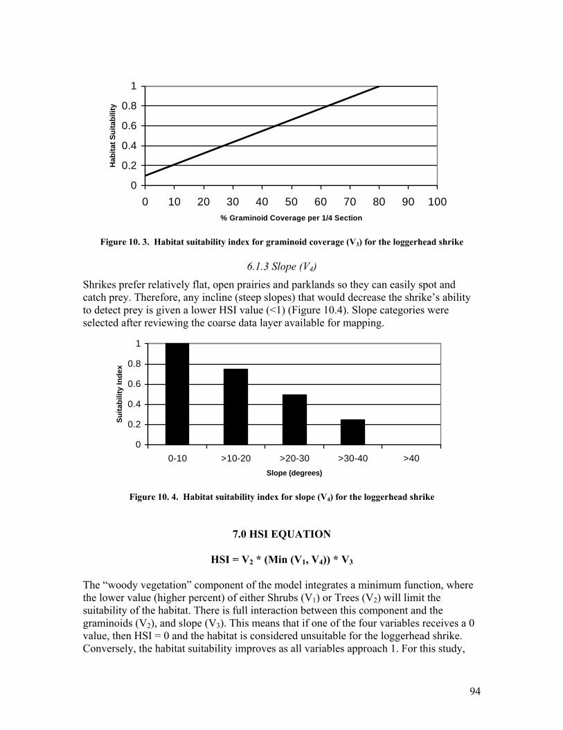
94
0
0.2
0.4
0.6
0.8
1
0 10 20 30 40 50 60 70 80 90 100% Graminoid Coverage per 1/4 Section
Hab
itat S
uita
bilit
y
Figure 10. 3. Habitat suitability index for graminoid coverage (V3) for the loggerhead shrike
6.1.3 Slope (V4)
Shrikes prefer relatively flat, open prairies and parklands so they can easily spot and catch prey. Therefore, any incline (steep slopes) that would decrease the shrike�s ability to detect prey is given a lower HSI value (<1) (Figure 10.4). Slope categories were selected after reviewing the coarse data layer available for mapping.
0
0.2
0.4
0.6
0.8
1
0-10 >10-20 >20-30 >30-40 >40Slope (degrees)
Suita
bilit
y In
dex
Figure 10. 4. Habitat suitability index for slope (V4) for the loggerhead shrike
7.0 HSI EQUATION
HSI = V2 * (Min (V1, V4)) * V3 The �woody vegetation� component of the model integrates a minimum function, where the lower value (higher percent) of either Shrubs (V1) or Trees (V2) will limit the suitability of the habitat. There is full interaction between this component and the graminoids (V2), and slope (V3). This means that if one of the four variables receives a 0 value, then HSI = 0 and the habitat is considered unsuitable for the loggerhead shrike. Conversely, the habitat suitability improves as all variables approach 1. For this study,

95
the ¼ sections containing at least 80% graminoids, 20% or less tress and 5%-30% shrubs on flat terrain would be ideal loggerhead shrike habitat. Conversely, as slope, percent tree cover, and percent shrub cover increases the habitat suitability of the site decreases.
7.1 Other Variables Considered
7.1.1 Grass Heights
There was no available database containing information on grass heights. This variable would have been useful in identifying areas of tall vegetation adjacent to short vegetation; transition zones favoured by shrikes for hunting.
7.1.2 Shrub Complexes
Being able to identify whether there are several single shrubs scattered throughout a ¼ section, a few hedgerows, or a dense clump of shrubs/trees would allow more precise modelling of loggerhead shrike habitat. The highest HSI values would have been assigned to ¼ sections containing small scattered clumps of shrubs or hedgerows/ shelterbelts, based on the preferred habitat for shrikes in southeastern Alberta for nesting and hunting (Collister 1994). Unfortunately, this data layer does not exist for the SHARP area
7.1.3 Farmyards
Farmyards within a sea of cultivation can act as island refuges for shrikes and other shrub nesting birds. Most farmyards provide edge habitat, consisting of grassland and cultivation separated by hedgerows. This data layers was unavailable for the SHARP project area.
8.0 FUTURE MANAGEMENT/RECOMMENDATIONS Increasing suitable loggerhead shrike habitat can be achieved through a variety of means: 1) The addition of at least one patch of thorny buffaloberry or willow per ¼ section in suitable locations can improve habitat (Telfer 1992). 2) Land management practices that promote heterogeneous herbaceous vegetation heights rather than intensive grazing.
9.0 HABITAT SUITABILITY MAP Please refer to map 10.1 for a cartographic representation of potential habitat for the loggerhead shrike within the Southern Headwater at Risk Project area.

96
10.0 LITERATURE CITED Alberta Sustainable Resource Development. 2001. The General Status of Alberta Wild
Species 2000. Alberta Sustainable Resource Development, Fish and Wildlife Service, Edmonton, AB. 46 pp. Publ. No. I/023.
Bjorge, R.R., and D.R.C. Prescott. 1996. Population estimate and habitat
associations of the Loggerhead Shrike, Lanius ludovicianus, in southeastern Alberta. Canadian Field-Naturalist 110(3): 445-449.
Brooks, B.L., and S.A. Temple. 1990. Habitat availability and suitability for loggerhead shrikes in the upper Midwest. American Midland Naturalist 123: 75-83.
Chabot, A.A.1994. Habitat selection and reproduction biology of the loggerhead shrike in Eastern Ontario and Quebec. Unpublished M. Sc. thesis. Macdonald Campus of McGill University. Montreal, Quebec. 161 pp.
Collister, D.M. 1994. Breeding ecology and habitat preservation of the Loggerhead
Shrike (Lanius ludovicianus) in southeastern Alberta. Unpublished M.Sc. thesis. University of Calgary, Calgary Alberta. 161 pp.
Collister, D.M. 1996. 1996 Population survey of loggerhead shrike, Lanius ludovicianus
excubitorides, nesting pairs Bassano subdivision- Atlee to Cavendish. Unpublished Report. Alberta Environmental Protection, Edmonton, AB. 9 pp.
De Smet, K.D. 1993. Status of ferruginous hawk and loggerhead shrike recovery
efforts. Pp. 329-332 IN: Proceedings of the third prairie conservation and endangered species workshop. Edited by G.L. Holroyd, H.L. Dickson, M. Regnier, and H.C. Smith. Provincial Museum of Alberta Natural History Occasional Paper 19: 1-384.
De Smet, K.D., and M.D. Conrad. 1989. The Loggerhead Shrike in Manitoba, its status and habitat needs. Unpublished report, Manitoba Department of Natural Resources, Winnipeg, MB. 23 pp. + app.
Gawlik, D.E., and K.L. Bildstein.1993. Seasonal habitat use and abundance of loggerhead shrikes in South Carolina. Journal of Wildlife Management 57 (2): 352-357.
Johns, B., E. Telfer, M. Cadman, D. Bird, R. Bjorge, K. De Smet, W. Harris, D. Hjertaas, P. Laporte, and R. Pittaway 1994. National Recovery Plan for the Loggerhead Shrike, Report No. 7. Ottawa: Recovery of Nationally Endangered Wildlife Committee. 32 pp.

97
National Geographic.1999. Field Guide to the Birds of North America-Third edition. National Geographic Society. Washington, D.C. 480 pp.
Prairie Conservation Forum. 2000. Native Prairie Vegetation Baseline Inventory.
[Online] http://albertapcf.terraengine.com/classinfo.htm Accessed Dec. 18, 2002. Prescott, D.R.C., and D.M. Collister. 1993. Characteristics of occupied and unoccupied
Loggerhead Shrike territories in southeastern Alberta. Journal of Wildlife Management 57: 346-352.
Prescott, D.R.C., and R.R. Bjorge. 1999. Status of the Loggerhead Shrike (Lanius
ludovicianus) in Alberta. Alberta Environment, Fisheries and Wildlife Management Division, and Alberta Conservation Association, Wildlife Status Report No. 24, Edmonton, AB. 28 pp.
Smith, W.W. 1991. The loggerhead shrike in Alberta. Pp. 241-242 IN: Proceedings of the second prairie conservation and endangered species workshop. Edited by G.L. Holroyd, G. Burns, and H. C. Smith. Provincial Museum of Alberta Natural History Occasional Paper 15: 241-242.
Telfer, E.S. 1992. Habitat change as a factor in the decline of the western Canadian
Loggerhead Shrike, Lanius ludovicianus, population. Canadian Field-Naturalist 106 (3): 321-326.
Wershler, R.M. 1989. Nesting habitat and abundance of the Loggerhead Shrike (Lanius ludovicianus) in two key areas of southern Alberta. Unpublished report for World Wildlife Fund Canada and Alberta Fish and Wildlife. 27 pp.
Yosef, R., and T.C. Grubb, Jr. 1994. Resource dependence and territory size in
loggerhead shrikes ( Lanius ludovicianus ). The Auk 111 (2): 465-469.

98
Map 10. 1. Potential habitat for the loggerhead shrike in the SHARP area.

99
Vagrant Shrew (Sorex vagrans)
François Blouin Wildlife Consultant, Lethbridge, AB
1.0 PURPOSE AND LIMITATIONS
The purpose of this model is to indicate potential year-round habitat for the vagrant shrew (Sorex vagrans) within the Southern Headwaters at Risk Project area. As this is a landscape level model with coarse variables, it may not be directly applicable to other areas or for site-specific analysis. This model is based on literature search and expert opinion and has not been tested in the field.
2.0 GENERAL INFORMATION The vagrant shrew is greyish brown to reddish on the back and smoky gray ventrally. In Alberta it has been found to measure 92-110 mm in length with a tail of 42-56 mm (Smith 1993). It can be identified from its third maxillary unicuspid tooth, which is smaller than the fourth, the short medial tines of the upper incisors, and by the four or fewer friction pads on the hind foot toes (Smith 1993). It usually lives less than 16 months (Hawes 1977). It occurs in western North America from southern British Columbia south to northern California and east to southwestern Alberta, western Montana and Wyoming, Utah, western Colorado, eastern Arizona, and western New Mexico (Smith 1993, CWHR 1995). In Alberta, it has been found in the southwestern part of the province, from the West Castle area to Waterton Lakes National Park (WLNP) (Smith 1993, Wallis et al. 2002). The vagrant shrew is currently classified as �may be at risk� in Alberta (Alberta Sustainable Resource Development 2001).
3.0 GENERAL HABITAT ASSOCIATIONS Vagrant shrews have been found from sea level to elevations up to 3750 m in a variety of habitats (CWHR 1995). They appear to favour wetlands or open patchy areas of moist coniferous forests or alpine meadows near water (Banfield 1981, Terry 1981). In western British Columbia, vagrant shrews generally occurred in moder (type of medium humified humus) soils along seepage sites and periodic streams characterized by an edaphic association of western red cedar (Thuja plicata), red alder (Alnus rubra), vine maple (Acer circinatum), and swordfern (Polystichum munitum) (Hawes 1977). In Alberta, they were trapped in higher densities in a wet coniferous forest of the Lower Subalpine ecoregion, but were also present from the Foothills Parkland to the Upper Subalpine ecoregions (Smith 1993, Wallis et al. 2002). They do not appear to be limited to one seral stage or vegetation type (Terry 1981).
3.1 Food Vagrant shrews feed on invertebrates, including insects and their larvae, worms, slugs and snails, spiders, as well as fungi, roots, young shoot, and possibly seeds and other

100
shrews (Clothier 1955, Whitaker and Maser 1976, CWHR 1995). In the Huntington Lake area of California, a greater density and diversity of prey items were found in the thick mat of dead vegetation in the wet Salix-Scirpus habitat where vagrant shrews were found than in the surrounding dryer meadow and forest (Ingles 1961).
3.2 Cover This species does not tunnel in soil like some other shrews (Terry 1981). Instead, it finds cover and food in the thick mat of dead vegetation of moist habitats, and makes great use of voles (Microtus spp.) runways (Ingles 1961, Whitaker and Maser 1976). The abundance of this species was highly correlated to the mean depth of the soil organic layers in a western hemlock (Tsuga heterophylla) forest of Washington (Terry 1981).
3.3 Reproduction Vagrant shrews nest under logs, roots, or dense vegetation (CWHR 1995). They also use abandoned nests of voles, deer mice, and moles (Hooven et al. 1975). The most common nest materials in a western Oregon study were grass, moss, and leaves (Hooven et al. 1975).
4.0 SPECIAL HABITAT ASSOCIATIONS
4.1 Water The presence of water seems to be an important habitat feature for this species (CWHR 1995). This may relate to the greater abundance of food nearby (Ingles 1961), or the vagrant shrew�s competitive disadvantage in dryer areas when burrowing shrews are present (Terry 1981). However, Spencer and Pettus (1966) suggested that this shrew might respond more to the vegetation structure of marsh habitats rather than an actual physiological requirement for water to explain their presence in clear-cut areas. Inglis (1961) noted that vagrant shrews were absent in moist habitats when sufficient cover was lacking, even though food was abundant.
5.0 HABITAT AREA REQUIREMENTS In western British Columbia, the average home range size for non-breeding S. vagrans was 1039 m² (Hawes 1977). Territoriality during the non-breeding season appears to regulate populations at a time before prey resources become limiting. By the onset of reproduction, territoriality breaks down and S. vagrans start to wander further away, with home ranges increasing to 3258 m² and overlapping. Breeding males� home range are larger than females� (4343 m² vs 2233 m²) (Hawes 1977). Home range boundaries appeared to follow more closely those of neighbouring sympatric shrews rather than the actual habitat boundaries (Hawes 1977). No habitat area information is known for Alberta.

101
6.0 ASSOCIATED SPECIES
Vagrant shrews have been found associated with dusky shrews (Sorex obscurus), masked shrews (S. cinereus), dwarf shrews (S. nanus), water shrews (S. palustris), Trowbridge shrews (S. trowbridgii), pigmy shrews (Microsorex hoyi), shrew-moles (Neurotrichus gibbsi), meadow voles (Microtus pennsylvanicus), long-tailed voles (M. longicaudus), gray-tailed voles (M. canicaudus), montane voles (M. montanus), Townsend�s voles (M. townsendii), creeping voles (M. oregoni), deer mice (Peromyscus maniculatus), western jumping mice (Zapus princeps), Camas pocket gophers (Thomomys bulbivorus), Townsend�s moles (Scapanus townsendii), and Townsend�s chipmunks (Eutamias townsendii) (Clothier 1955, Inglis 1961, Spencer and Pettus 1966, Hooven et al. 1975, Hawes 1977, Terry 1981). In WLNP, it was trapped with deer mouse (Peromyscus maniculatus), dusky shrew (Sorex obscurus), masked shrew (S. cinereus), water shrew (S. palustris), heather vole (Phenacomys intermedius), long-tailed vole (Microtus longicaudus), meadow vole (M. pennsylvanicus), water vole (M. richardsoni), southern red-backed vole (Clethrionomys gapperi), northern bog lemming (Synaptomys borealis), and western jumping mouse (Zapus princeps) (Wallis et al. 2002).
7.0 THE HSI MODEL
7.1 Selected Habitat Variables Little information is available about habitat characteristics of the vagrant shrew in Alberta. Trapping in WLNP revealed that they occurred in densities of 1.25 - 2.50 individuals per 100 trap-nights in the Foothills Parkland ecoregion, 1.85 in the Montane ecoregion, 0.29 � 7.50 in the Lower Subalpine ecoregion, and 1.25 - 1.67 in the Upper Subalpine ecoregion. They did not occur in the alpine ecoregion (Wallis et al. 2002). For this model, it will be assumed that trapping densities are representative of the actual population densities in the various ecoregions. Smith (1993) mentions that specimens were collected along a mountain stream in a coniferous forest.
7.1.1 Natural Subregion (V1)
The ecoregions used by Wallis et al. (2002) are conceptually similar to the natural subregions of Achuff (1992). However, Wallis et al.�s (2002) data set covered only WLNP. In this model we assumed Wallis et al.�s (2002) ecoregions to be equivalent to Achuff�s (1992) natural subregions, with the �Lower Subalpine� and �Upper Subalpine� ecoregions combined to represent the Subalpine natural subregion. Since the highest density of vagrant shrews was trapped in this subregion, it was assigned a suitability value of 1. Maximum density values in all other subregions were divided by 7.5, the highest vagrant shrew density observed, and results used as suitability values. The Foothills Parkland natural subregion thus received a suitability value of 0.33 (2.50/7.50), the Montane subregion a value of 0.25 (1.85/7.50), while the Alpine subregion a value of zero (0/7.50). The Grassland natural subregions do not reach WLNP and thus were not sampled by Wallis et al. (2002). However, there is no evidence in the literature that

102
vagrant shrews occur in the prairie landscape. Foothills Fescue and Mixedgrass Prairie natural subregions were thus given a suitability value of zero (Figure 11.1).
0
0.2
0.4
0.6
0.8
1
MiixedgrassPrairie
FoothillsFescue
FoothillsParkland
Montane Subalpine Alpine
Natural Subregion
Suita
bilit
y In
dex
Figure 11. 1. Habitat suitability index for natural subregion (V1) for the vagrant shrew.
7.1.2 Ecological Moisture Regime (V2)
Vagrant shrews tend to be associated with damp habitats, either damp meadows, marshes, stream banks, riparian zones, and moist woods (Bailey 1918 in Clothier 1955, Jackson 1928 in Clothier 1955, Clothier 1955, Ingles 1961, Spencer and Pettus 1966, Hooven et al. 1975, Smith 1993). A hygric or subhydric moisture regime (moisture class �w� of the Alberta Vegetation Inventory; Nesby 1996) were thus given a suitability value of 1. A subhygric moisture regime was also considered suitable. However, this regime falls into the same broad moisture class �m� as the mesic and submesic regimes, which were considered unsuitable. For this reason, the moisture class �m� was given a suitability value of 0.3 to account for the one moisture regime category considered suitable in this class of three. Both the xeric (class �d�) and hydric (class �a�) were considered unsuitable and were given a suitability value of zero (Figure 11.2).
0
0.2
0.4
0.6
0.8
1
d m w a
Moisture Regime Class
Suita
bilit
y In
dex
Figure 11. 2. Habitat suitability index for ecological moisture regime (V2) for the vagrant shrew.

103
7.1.3 Distance from Water (V3)
Shrews are never found far from water (Clothier 1955). Spencer and Pettus (1966) in Colorado captured them at an average of 18.9 ± 4.0 m (61.9 ± 13.1 ft) to the nearest permanent surface water. In this case, the mode would have been a more valuable statistic but was not available. However, it can be derived that 58% of the vagrant shrews were trapped at the water�s edge. In western Montana, vagrant shrews were taken at a distance less than 183 m (600 ft) from small and large creeks, irrigation ditches, small standing pools, and lakes, but by far, the most vagrant shrews were taken near water (Clothier 1955). A negative linear relationship was thus favoured between the distance from water and the suitability value. The suitability value was set to decrease from 1 at 0 m from open water to 0 at 183 m (Figure 11.3).
0
0.2
0.4
0.6
0.8
1
0 15 30 45 60 75 90 105 120 135 150 165 180Distance from Water (m)
Suita
bilit
y In
dex
Figure 11. 3. Habitat suitability index for distance from water (V3) for the vagrant shrew.
7.1.4 Crown Closure Class (V4)
Terry (1981) found that Sorex vagrans was negatively correlated to percent shrub cover and to tall tree cover and noted that it was rare in closed forests but common in open patchy areas such as alder stands and forest meadows. According to the Alberta Vegetation Inventory, crown closure or density class applies only to forested land (Nesby 1996). Non-forested land (NFL) classified as herbaceous grassland (HG), herbaceous forbs (HF), or undifferentiated open shrub (SO), were thus assigned a suitability value of 1. Forested land (> 6% crown closure) of density class �A� (6 - 30% crown closure) was assigned a suitability value of 0.8, class �B� (31 � 50%) a value of 0.6, class �C� (51 � 70%) a value of 0.4, and class �D� (71 � 100%) a suitability value of 0.2. Class �D� was not assigned a suitability value of 0, since some vagrant shrews have been detected in low densities in various forested habitats (Spencer and Pettus 1966, Hooven et al. 1975, Hawes 1977, Terry 1981, Smith 1993, Wallis et al. 2002). The non-forested land

104
classified as �undifferentiated closed shrub� (SC) was similarly given a suitability value of 0.2. All other classes were given a value of 0 (Figure 11.4).
0
0.2
0.4
0.6
0.8
1
OTHERNFL
HG/HF/SO A B C D SC
Crown Closure Class
Suita
bilit
y In
dex
Figure 11. 4. Habitat suitability index for crown closure class (V4) for the vagrant shrew.
8.0 HSI EQUATION
HSI = V1 * V4 * (V2 +V3) The variables are non-compensatory but there is interaction between V1 (natural subregion), V4 (crown closure) and the other two variables. A suitable moisture regime (V2) or distance from water (V3) in an unsuitable natural subregion or crown closure class would result in an unsuitable habitat for the vagrant shrew. In addition, there is a cumulative relationship with no interaction between V2 and V3. Either suitable moisture regime or distance from water will provide suitable habitat for the vagrant shrew, assuming that the other two variables are not zero.
9.0 SOURCES OF OTHER MODELS One other habitat suitability model for the vagrant shrew was developed by the California Wildlife Habitat Relationships (CWHR) System for use with their habitat types maps (CWHR 1995).
10.0 HABITAT SUITABILITY MAP Please refer to map 11.1 for a cartographic representation of potential habitat for the vagrant shrew within the Southern Headwater at Risk Project area.

105
11.0 LITERATURE CITED Achuff, P.L. 1992. Natural regions, subregions and natural history themes of Alberta: A
classification for protected areas management. Report No.2. Prepared for Parks Services and Natural and Protected Areas, Alberta Government. Revised and updated December 1994.
Alberta Sustainable Resource Development 2001. The general status of Alberta wild
species 2000. Alberta Sustainable Resource Development, Fish and Wildlife Service. Edmonton, AB. 46 pp. Pub. No. I/023.
Bailey, V. 1918. Wild animals of Glacier National Park, the mammals. U.S. Government
Printing Office. Washington, D.C. 102 pp. Banfield, A.W.F. 1981. The mammals of Canada. University of Toronto Press. National
Museum of Natural Sciences; National Museums of Canada. Toronto, ON. 438 pp.
California Wildlife Habitat Relationship Program (CWHR). 1995. Habitat suitability
models for use with Arc Info: vagrant shrew. California Department of Fish and Game. CWHR Technical Report No. 23. Sacramento, CA. 10 pp + appendix.
Clothier, R.R. 1955. Contribution to the life history of Sorex vagrans in Montana. J.
Mammal. 36: 214-221. Hawes, M.L. 1977. Home range, territoriality, and ecological separation in sympatric
shrews, Sorex vagrans and Sorex obscurus. J. Mammal. 58: 354-367. Hooven, E.F., Hoyer, R.F., and R.M. Storm. 1975. Notes on the vagrant shrew, Sorex
vagrans, in the Willamette Valley of Western Oregon. Northwest Sci. 49: 455-462.
Ingles, L.G. 1961. Home range and habitats of the wandering shrew. J. Mammal. 42:
455-462. Jackson, H.H.T. 1928. A taxonomic review of the American long-tailed shrew. North
Amer. Fauna No. 51. 238 pp. Nesby, R. 1996. Alberta Vegetation Inventory Standards Manual v. 2.2. Alberta
Environment Protection. Unpublished Document. 42 pp + appendices. Smith, H. C. 1993. Alberta mammals: an atlas and guide. Provincial Museum of Alberta.
Edmonton, AB. 239 pp. Spencer, A.W., and D. Pettus. 1966. Habitat preferences of five sympatric species of
long-tailed shrews. Ecology. 47: 677-683.

106
Terry, C.J. 1981. Habitat differentiation among three species of Sorex and Neurotrichus
gibbsi in Washington. Amer. Midl. Nat. 106: 119-125. Wallis, C., Wershler, C., and R. Riddell. 2002. Ecological land classification of Waterton
Lakes National Park, Alberta. Vol. II: wildlife resources. Parks Canada, Waterton Park, Alberta. 258 pp.
Whitaker, J.O.Jr., and C. Maser. 1976. Food habits of five western Oregon shrews.
Northwest Science 50: 102-107.

107
Map 11. 1. Potential habitat for the vagrant shrew in the SHARP area.

108
Grizzly Bear (Ursus arctos)
Carita Bergman Alberta Fish and Wildlife Division, Pincher Creek, AB
1.0 PURPOSE AND LIMITATIONS The purpose of this modeling exercise is to identify variation in grizzly bear habitat suitability across the Southern Headwaters At Risk Project (SHARP) study area. This model is based largely on that created for grizzly bears during the Southern Rockies Landscape Pilot Planning Process (SRLPPP; Alberta Environmental Protection 1998). In contrast to the original model, this version incorporates locational data collected from radio-tracking of 11 grizzly bears collared during captures at bear-human conflict sites in southwest Alberta, and subsequently released within the area. In addition, temporally limited but frequent relocations from two research bears collared in the vicinity of the Crowsnest Pass are included in the dataset. HSI models are often constructed in the absence of data relevant to the local area. It should be noted that this model is based, at least in part, on real data collected in the study area of interest, though these data are limited in their resolution by their infrequent collection over time periods ranging from a few months to several years. While other habitat models for grizzly bears exist (some for the area of study, some for elsewhere), they were not selected for a variety of reasons: Miistakis Institute model (2002): this model uses course habitat cover types (e.g. �forest� versus the many types of forest identified by AVI/SAS), and only covers the Castle watershed area; some areas have large amounts of missing habitat data. Carroll et al. (2000): this model is not appropriate for small-scale management (P. Paquet, personal communication). SRLPPP grizzly bear HSI: this model does not cover southern portion of SHARP study area, is based on incomplete eco-site phase data that cannot be derived for the southern area, and uses food values (Kansas et al. 1995) based on work from Banff/Jasper that are inappropriate for the local area (M. Gibeau & G. Stenhouse, personal communication). Use of the current model is considered interim, useful only until more rigourous modeling efforts are completed. Provincial efforts to create ground-truthed habitat maps linking cover types with vegetative productivity will be completed in the upcoming year. A habitat model developed by the Alberta Foothills Model Forest grizzly bear research program is being validated for the area through the collection and application of local grizzly bear locational data, an exercise that will be completed in one to two years. When complete, this new model will replace that developed here.

109
2.0 GENERAL INFORMATION Grizzly bears are a wide-roaming species that once ranged across the Canadian prairies, but are now restricted to mountainous and tundra areas as their North American range contracted with expansion of human activities and impact. Clearly, they are susceptible to habitat loss and high mortality in areas of high human activity, and concern for long-term persistence is apparent over much of their southern range. Grizzly bears are considered to be a good indicator or umbrella species for wide-ranging carnivores, because of their requirements for large, secure spaces and their sensitivity to high mortality.
3.0 THE HSI MODEL
3.1 Habitat Preference Index Other work (e.g. Alberta Environmental Protection 1998) addressing habitat modeling for grizzly bears often separates pre- and post- berry seasons. For land use recommendations, these separate models are often combined (Stenhouse, personal communication). Here, by using coarse data collected over both pre- and post- berry seasons, I effectively combine these two seasons while losing the level of resolution necessary to separate within-season variation. Using a 100% convex polygon derived from pooled grizzly bear relocation data, habitat availability within the polygon was measured in a GIS environment using the draft vegetation base layer from the Southern Alberta Strategy (provided by the Resource Data Division, spatial analysis completed by Vernon Remesz). The percent occurrence (i.e. area) of each habitat type was defined as �available� habitat to grizzly bears in the SHARP study area. For individual bears, locations were allocated to a specific habitat type by noting the predominant habitat type within a 50m buffer of each location. The analysis was repeated with buffers up to 500m, with similar results. The probability of occurrence in each habitat type for each bear was then determined, and with the availability data, a preference index was calculated using Ivlev�s index (Krebs 1989). Ivlev�s index ranges between �1 and +1, with positive values indicative of preference, and negative values indicative of avoidance. Ivlev values were then converted to Habitat Preference Index (HPI) values. Highly preferred habitat types (Ivlev value >0.5) were given the highest habitat preference index value of 5. Low preference habitat types (0<Ivlev value<0.5) were given a habitat value of 4. Habitat types for which no preference or avoidance was shown (Ivlev value = 0) were given a habitat value of 3. Moderate avoidance (-0.5<Ivlev value<0) warranted assignment of a value of 2, while extreme avoidance (Ivlev value < -0.5) received a value of 0. By giving habitats which appeared to be mildly avoided (although potentially greatly used, as �pine�) a positive value of two, I allowed for value for these habitats that were either generally avoided by most individual bears, but selected by a few, or were

110
highly abundant but used less than expected (e.g. �pine�). Mean HPI values were then calculated for each habitat type, using the individual bear as the sampling unit (Table 12.1). Table 12. 1. Total bears in each HPI category, with mean HPI value listed on the far right. Cover types listed on the left are from the draft vegetation base layer used in the Southern Alberta Strategy. The weighed mean HPI value (HPI (w)) was obtained by dividing the mean HPI by the highest mean HPI value observed.
Cover Type V-HIGH = 5 HIGH = 4 MED = 3 LOW = 2 V-LOW = 0 MEAN HPI HPI (w)White Spruce 8 3 0 0 2 4.0 1.00
Spruce Fir 8 1 0 0 4 3.4 0.85 Hardwood 7 1 0 0 5 3.0 0.75
Douglas Fir 3 5 0 1 4 2.8 0.70 Forest Shrub 6 1 0 0 6 2.6 0.65 Mixedwood 6 0 0 0 7 2.3 0.58
Riparian Wetland 5 0 0 0 8 1.9 0.48 Grassland 0 2 0 7 4 1.7 0.43
Crops 1 4 0 0 8 1.6 0.40 Pine 0 1 0 6 6 1.2 0.30
Rock Ice 0 2 0 3 7 1.1 0.28 Foothills Parkland 2 0 0 0 11 0.8 0.20
Water 0 2 0 0 11 0.6 0.15 Agricultural Residential 1 0 0 0 12 0.4 0.10
Central Parkland 1 0 0 0 12 0.4 0.10 Major Road 0 0 0 1 12 0.2 0.05
Foothills Fescue 0 0 0 0 13 0.0 0.00 Industrial 0 0 0 0 13 0.0 0.00
Rural Residential 0 0 0 0 13 0.0 0.00 Surface Pit 0 0 0 0 13 0.0 0.00 Town City 0 0 0 0 13 0.0 0.00
3.2 Zones and Degrees of Human Influence Following Alberta Environmental Protection (1998),
�Distance from cover as well as the presence of access (roads, trails, etc.) and other aspects of human use greatly alter the effectiveness of grizzly bear habitat. Various man made [sic] features and human activities have differing zones and degrees of human influence. The proximity to other land uses/features as well as the presence or absence of cover will also influence habitat effectiveness. The suitability (SI) values for each land use or access type are coefficients with a value between 0 and 1 that reflect the degree to which habitat is reduced in value by the presence of
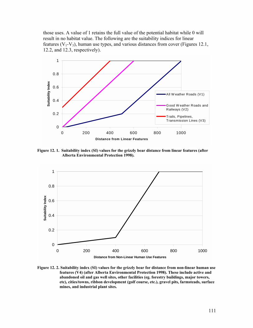
111
those uses. A value of 1 retains the full value of the potential habitat while 0 will result in no habitat value. The following are the suitability indices for linear features (V1-V3), human use types, and various distances from cover (Figures 12.1, 12.2, and 12.3, respectively).
0
0.2
0.4
0.6
0.8
1
0 200 400 600 800 1000Distance from Linear Features
Suita
bilit
y In
dex
All W eather Roads (V1)
Good W eather Roads andRailways (V2)
Trails, Pipelines,Transmission Lines (V3)
Figure 12. 1. Suitability index (SI) values for the grizzly bear distance from linear features (after
Alberta Environmental Protection 1998).
0
0.2
0.4
0.6
0.8
1
0 200 400 600 800 1000Distance from Non-Linear Human Use Features
Suita
bilit
y In
dex
Figure 12. 2. Suitability index (SI) values for the grizzly bear for distance from non-linear human use
features (V4) (after Alberta Environmental Protection 1998). These include active and abandoned oil and gas well sites, other facilities (eg. forestry buildings, major towers, etc), cities/towns, ribbon development (golf course, etc.), gravel pits, farmsteads, surface mines, and industrial plant sites.

112
Again, from Alberta Environmental Protection (1998):
�One type of cover is recognized; vegetative. Topographic cover is not utilized at present. Vegetation is considered cover if it is at least 3 metres tall and has a density class of B or greater (over 31% crown closure; Nesby 1996). If the habitat is within 200m of cover it retains its full value (1). At 500m from cover the value is reduced to 0.8 of its value while at 1000m the value is reduced to 0.2 of the original calculation (Figure 12.3).� Since forest cover exists outside the extent of the AVI database (Figure 1.2 a), the draft vegetation base layer �cover type� variable (see Table 12.1) and the NPVI (Figure 1.2 b) �percent tree cover� variable were combined together with the AVI �density class� variable to obtain a full coverage of the SHARP area for V5. The polygons from the draft vegetation base layer classified as �Douglas Fir�, Hardwood�, �Mixedwood�, �Pine�, �White Spruce�, or �Spruce/Fir� were all assumed to be at least 3 metres tall and of ≥ 31% or crown closure. The NPVI polygons with greater than 30% tree cover were also assumed to be at least 3 metres tall.
0
0.2
0.4
0.6
0.8
1
0 200 400 600 800 1000Distance from cover
Suita
bilit
y In
dex
Figure 12. 3. Suitability index (SI) value for distance from cover (V5) (after Alberta Environmental
Protection 1998).
3.3 Spatial Arrangement of Habitat Patches One of the central tenets of optimal foraging theory is that the value of a habitat patch is in part dictated by the travel cost of reaching that patch (Stephens and Krebs 1986). Thus, a patch surrounded by other good quality patches is necessarily of higher value than the same patch if it were surrounded by only poor quality habitat patches. To incorporate this idea into the HSI model, initial patch value calculated from other variables is determined for each pixel. Then, an average of all the pixels within a daily foraging area (9 km2) is calculated, and reassigned as the final value to the central pixel.

113
4.0 HSI EQUATION COMPONENTS
For each pixel of habitat, the following equations apply for obtaining the final HSI value:
initial foraging value = HPI (w) * [V1 * V2 * V3 * V4 * V5 ]
HSI = AVERAGE (initial foraging values of surrounding pixels in 9 km2)
6.0 HABITAT SUITABILITY MAP Please refer to map 12.1 for a cartographic representation of potential habitat for the grizzly bear within the Southern Headwater at Risk Project area.
7.0 SELECTED REFERENCES Alberta Environmental Protection. 1998. The Southern Rockies Landscape Planning Pilot
Study: Summary Report. Alberta Environmental Protection, Lands and Forest Service (Olson and Olson).
Carroll, C, PC Paquet and RF Noss. 2000. Modelling carnivore habitat in the Rocky
Mountain region: a literature review and suggested strategy. World Wildlife Fund, Toronto, Ontario.
Kansas, JL and RN Ridell. 1995. Grizzly bear habitat model for the four contiguous
mountain parks (second iteration), Parks Canada. Krebs, CJ. 1989. Ecological Methodology. Harper and Rowe, New York. 654 pp. Miistakis Institute for the Rockies. 2002. Transboundary cumulative effects analysis for
the grizzly bear. Unpublished report, Miistakis Institute for the Rockies, Calgary, Alberta.
Nesby, R. 1996. Alberta Vegetation Inventory � Standards Manual. Final Draft, Version
2.2. Data Acquisition Branch, Resource Data Division, Alberta Environmental Protection. Unpublished document. 42 pp. + appendices.
Stephens, DW and JR Krebs. 1986. Foraging Theory. Princeton University Press,
Princeton, NJ, USA. USDA Forest Service. 1990. CEM � A model for assessing effects on grizzly bears. US
Dept. of Agric. Forest Service. Missoula, Montana.

114
Map 12. 1. Potential habitat for the grizzly bear in the SHARP area.

115
Wolverine (Gulo gulo)
Michael Jokinen Alberta Conservation Association, Blairmore, AB
1.0 PURPOSE AND LIMITATIONS
The purpose of this habitat suitability index model is to distinguish potential wolverine (Gulo gulo) habitat within the Southern Headwaters at Risk Project (SHARP) area. The wolverine model is based on coarse variables at the landscape level and may not be directly applicable to other areas or for site-specific analysis. This model is based on published and unpublished literature and expert opinion, and has not been field-tested.
2.0 GENERAL INFORMATION
2.1 Status The wolverine rated high as a Species At Risk (SAR) in the SHARP area. In eastern Canada, the wolverine is listed as endangered by COSEWIC (2003) and the western population is of special concern. The wolverine is a managed fur-bearing animal in Alberta and is subject to trapping. Alberta Sustainable Resource Development (2001) believes the Alberta wolverine may be at risk due to the reduced harvests over the years. Trapper harvest data in the province show a steady decline in pelt numbers since 1984 (Peterson 1997). Peterson (1997) mentions that this is not an accurate measure because several factors can be responsible for the lower harvest rates. Wolverines are highly susceptible to trapping because of their scavenging nature and keen sense of smell (Hornocker and Hash 1981) making them vulnerable to trap baits. Trapping has the ability to quickly eradicate local wolverine populations if they were not managed with a quota system. Alberta�s wolverine quota allows for one wolverine harvest per trap line, per year. The trapping season in the SHARP area is November 1-January 31 when a wolverine pelt is at its prime. A prime pelt is when the new guard hair and under-fur of the wolverine have reached maximum growth (Stains 1979). Wolverine pelts were worth $263.20 in 2002/2003, but the majority are being sent to taxidermists rather than for the sale of fur because of its rarity and higher price once mounted (Triechel pers comm. 2003).
2.2 Distribution The circumpolar distribution of the wolverine includes Canada, Estonia, Finland, Norway, Sweden, Russia, Mongolia and the United States (Whitman et al. 1986). In Canada, they are found in the northern forested areas, the alpine habitats of the western Rockies and on the arctic tundra (COSEWIC 2003). They are quite rare in Labrador, Quebec and Ontario. In Manitoba and Saskatchewan they are confined to the extreme northern regions, while in Alberta they are located in the northern part of the province and along its western border in the Rocky Mountains (van Zyll De Jong 1975). Alberta trapping harvest data reveal high population densities in the north western portion of the

116
province (Peterson 1997). Population studies in British Columbia and the Territories indicate population trends that are stable (van Zyll De Jong 1975) but the Vancouver Island population may already be extinct (COSEWIC 2003). In areas of Europe, the wolverine is protected. For example, the wolverine has been a protected species since 1968 throughout all of Sweden. It has also been protected in the southern half of Norway since 1973 and all of Norway since 1982 (Landa et al. 1997). North America�s southernmost wolverine populations occur in the interior north western states (Rowland et al. 2003). According to Hornocker and Hash (1981) Montana is the only state with a viable population even though the wolverine was nearly extinct in the state by the 1920�s (Newby and Wright 1955).
2.3 General Description The wolverine is the largest terrestrial member of the weasel (Mustelid) family. It does not possess the general long and lean features of a weasel, but rather a broad and sturdy, bear-like stature. Males are larger than females (Moors 1980) at an average of 12-14 kilograms and 8-10 kilograms respectively (Wolverine Foundation 2003, Pattie and Fisher 1999). The wolverine has very strong jaws, well-developed neck and shoulder muscles and long claws. It uses these adaptations when feeding on frozen flesh and crushing large bones and when digging for prey through frozen soil or climbing trees (Boles 1977). Except for the hyena (Crocuta crocuta), no other mammal has a stronger bite than the wolverine (Discovery Communications Inc. 1998). Some potential wolverine predators are eagles (Aquila chrysaetos, Haliaeetus leucocephalus), bears (Ursus sp.), cougar (Puma concolor) and wolves (Canis lupus) (Hornocker and Hash 1981). Boles (1977) documented wolves killing wolverines in the arctic, where the wolverine was unable to escape due to the open terrain. In Latin, the name Gulo gulo means �Glutton glutton� and the wolverine likely acquired this name for the legendary tales of attacking human food caches or dwellings in the backcountry, making a mess and producing an unpleasant odour (Gadd 1995). Wolverines scent mark, by releasing musk, maintaining spacing in time but not area (Koehler et al. 1980). Wolverines are not territorial, (Hornocker and Hash 1981) thus, scent marking may indicate that an area is being hunted and inefficient for other wolverines searching for prey. They will mark up to 20 sites within 2.5 kilometers of travel and will change their travel direction to investigate a marked site (Koehler et al. 1980). Koehler et al. (1980) discovered four wolverine-marking behaviors. The most common behavior includes clawing and tree climbing, depositing musk on the trunk and ground at an average height of 46 centimeters. The marked tree was typically a large, prominent pine in the area. Wolverines will also scratch the soil surface, gnaw a tree limb scented with musk or deposit scat or musk on the ground with no other visual signs. These marking sites are well established and used year after year (Koehler et al. 1980). Wolverines will mark carcasses but Discovery Communications Inc. (1998) states that they are only likely to scent mark a carcass if they are threatened while feeding at the carcass.
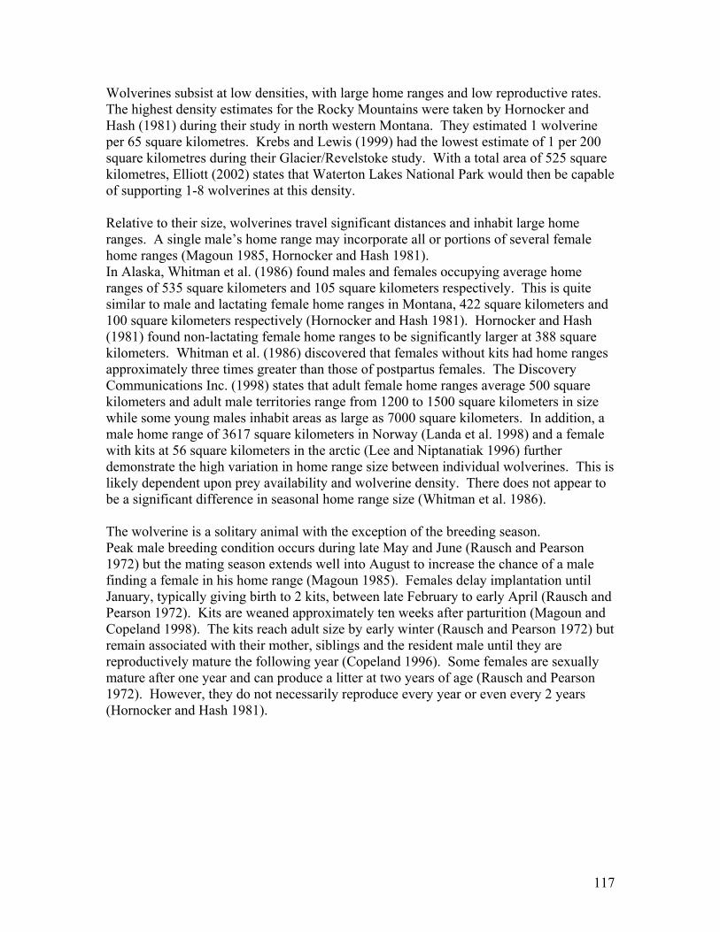
117
Wolverines subsist at low densities, with large home ranges and low reproductive rates. The highest density estimates for the Rocky Mountains were taken by Hornocker and Hash (1981) during their study in north western Montana. They estimated 1 wolverine per 65 square kilometres. Krebs and Lewis (1999) had the lowest estimate of 1 per 200 square kilometres during their Glacier/Revelstoke study. With a total area of 525 square kilometres, Elliott (2002) states that Waterton Lakes National Park would then be capable of supporting 1-8 wolverines at this density. Relative to their size, wolverines travel significant distances and inhabit large home ranges. A single male�s home range may incorporate all or portions of several female home ranges (Magoun 1985, Hornocker and Hash 1981). In Alaska, Whitman et al. (1986) found males and females occupying average home ranges of 535 square kilometers and 105 square kilometers respectively. This is quite similar to male and lactating female home ranges in Montana, 422 square kilometers and 100 square kilometers respectively (Hornocker and Hash 1981). Hornocker and Hash (1981) found non-lactating female home ranges to be significantly larger at 388 square kilometers. Whitman et al. (1986) discovered that females without kits had home ranges approximately three times greater than those of postpartus females. The Discovery Communications Inc. (1998) states that adult female home ranges average 500 square kilometers and adult male territories range from 1200 to 1500 square kilometers in size while some young males inhabit areas as large as 7000 square kilometers. In addition, a male home range of 3617 square kilometers in Norway (Landa et al. 1998) and a female with kits at 56 square kilometers in the arctic (Lee and Niptanatiak 1996) further demonstrate the high variation in home range size between individual wolverines. This is likely dependent upon prey availability and wolverine density. There does not appear to be a significant difference in seasonal home range size (Whitman et al. 1986). The wolverine is a solitary animal with the exception of the breeding season. Peak male breeding condition occurs during late May and June (Rausch and Pearson 1972) but the mating season extends well into August to increase the chance of a male finding a female in his home range (Magoun 1985). Females delay implantation until January, typically giving birth to 2 kits, between late February to early April (Rausch and Pearson 1972). Kits are weaned approximately ten weeks after parturition (Magoun and Copeland 1998). The kits reach adult size by early winter (Rausch and Pearson 1972) but remain associated with their mother, siblings and the resident male until they are reproductively mature the following year (Copeland 1996). Some females are sexually mature after one year and can produce a litter at two years of age (Rausch and Pearson 1972). However, they do not necessarily reproduce every year or even every 2 years (Hornocker and Hash 1981).

118
3.0 HABITAT ASSOCIATIONS
3.1 Diet The wolverine diet varies seasonally, regionally and with availability. The wolverine is an optimal seasonal scavenger that is dependent upon the main links of the food web (Van Zyll de Jong 1975, Hornocker and Hash 1981) and is likely more influenced by food availability than specific habitat features (Hornocker and Hash 1981). For these reasons, associating the wolverine to a particular habitat is a complicated, time consuming and site-specific issue and should be dealt with regionally with a focus on international connectivity. During the summer, the wolverine will eat a wide variety of prey such as ground squirrels (Spermophilus sp.), marmots (Marmota sp.) (Lofroth 2001), porcupines (Erethizon dorsatum), blueberries (Vaccinium sp.), microtines (Rausch and Pearson 1972), snowshoe hare (Lepus americanus), other mustelids, beavers (Castor canadensis), avian species, domestic cow (Bos taurus), horse (Equus caballus) (Hornocker and Hash 1981) and even whitebark pine (Pinus albicaulis) seeds (Heinemeyer et al. 2001). Some studies found a high frequency of beaver in the wolverine diet but this is likely a result of feeding on trapper baits (Lofroth 2001). Wolverines will dig food caches beneath remnant snowdrifts during summer months (Magoun and Copeland 1998) to preserve foods for periods when food sources are scarce. They are polyphagous, enabling them to switch between food sources as one becomes scarce (Landa et al. 1997). Wolverines will even cannibalize one another (Lofroth 2001, Flook and Rimmer 1965). Rodentia mammals may be the most important food source during the summer (Magoun 1987). Wolverines have increased reproductive success during years of peak rodent cycles (Landa et al 1997). Females may prefer small prey so their reproductive efficiency is improved (Moors 1980). During the spring, Hornocker and Hash (1981) found wolverines spending significant time in areas where ground squirrels were plentiful. Squirrels are most vulnerable in early spring when mating, but were also the most important food item in the wolverine diet during August when the squirrels dispersed (Magoun 1987). Summer scats revealed a 58% arctic ground squirrel, 18% other small mammal and 18% caribou and egg fecal composition (Magoun 1987). Ground squirrels are also an important part of the winter diet. Magoun (1987) observed wolverines digging ground squirrels out of the frozen ground while they were hibernating. During the winter, wolverines still feed on small rodents, hares and ptarmigan (Lagopus sp.) but they mainly rely on scavenging for large ungulate (Bovidae and Cervidae sp. ) carrion (Landa et al. 1997). The wolverine is well adapted for carrion feeding, using its strong jaws to feed on frozen meat and crush large bones (Hornocker and Hash 1981). Wolverines would not survive without large ungulate populations (Magoun 1985) because they play a very important role in the wolverine diet (Banci 1987, Copeland 1996, Gardner 1985, Magoun 1987). Van Zyll de Jong (1975) states that wolverine abundance is related to the biomass and turnover of large ungulate populations.

119
Wolverines are still fairly common in the mountain ranges of Alberta, British Columbia and the Yukon and these areas possess large and diverse ungulate populations. Swedish/Scandinavia wolverine populations are considered sympatric with caribou (Rangifer tarandus) (Persson 2003, Landa et al. 1997). A decline in caribou and wolf populations in certain areas have caused a decline in wolverine numbers because of the lack in carrion and a lack of predators leaving carrion behind (van Zyll De Jong 1975). In Europe, humans and wolverines come into conflict with domestic sheep herding because they prey on the domestic sheep. They impact sheep populations by preying on the domestic lambs (Landa et al. 1997), and are responsible for a 40% lamb loss during the summer (Landa and Tommeras 1997). The wolverine has adapted to winter survival and is capable of using the snow to its advantage when hunting and scavenging. This morphological adaptation to having a low weight load in deep snow makes the wolverine a great winter predator. Only the caribou and moose (Alces alces) have higher snow foot loadings than the wolverine (Telfer and Kelsall 1984,van Zyll De Jong 1975), leaving deer (Odocoileus sp.), elk (Cervus elaphus), goats (Oreamnos americanus) and sheep (Ovis sp.) at a disadvantage in deep snow. Wolverines will also enter tree wells in winter in search for rodents and take hibernating marmots under snow burrows. They have a keen sense of smell and thus are able to locate food under deep snow. Some wolverines have traveled more than 3 kilometers to baited areas (Hornocker and Hash 1981). They have also adapted to following tracks of other predators in search of carrion but this behaviour can increase the chance of injury or cause death since they are scavenging kills of other carnivores (Copeland 1996). These larger and more efficient carnivores may be essential to the wolverine for a winter supply of carrion. Wolverines are such efficient scavengers that they are able to live on only bone and hide remnants during periods of food scarcity. Some scat analyses in Alaska have consisted of only chalky bone matter (Magoun 1987). A wolverine retrieving summer food caches during the winter season produced scats with significant amounts of soil and squirrel remains (Magoun 1987). An adult wolverine is able to survive harsh winters by scavenging and caching foods but a wolverine�s reproductive potential is then likely sacrificed (Magoun 1985). Even though the wolverine is well adapted to winter survival, starvation and predation are the primary causes of death in weaned wolverines (Hornocker and Hash 1981). Thus, the availability of food is the primary factor determining if a wolverine population will persist in any given area.
3.2 Denning Habitat Associating the wolverine to a specified habitat is an arduous task because of its scavenging nature and nomadic behaviour. The only time period that a wolverine demonstrates site fidelity to a specified habitat type is during the denning period when an adult female is caring for her young (Magoun and Copeland 1998, Landa et al. 1998). Optimal denning habitat attributes would include appropriate vegetative communities that support a sufficient prey base year round and suitable landscape features for den formation. The denning period occurs between February and April (Magoun and Copeland 1998). Dens are usually located in lower to upper subalpine, cirque basins and

120
avalanche slopes. They are located among large boulder talus or downed woody debris and are rarely reported in low elevation densely forested areas (Copeland 1996, Krebs and Lewis 1999, Landa et al. 1998, Magoun and Copeland 1998). In Idaho, dens reach snow-covered boulder talus in open subalpine cirque basins. They were located above 2500 meters in elevation and were generally surrounded by trees on north facing slopes (Magoun and Copeland 1998). Wolverines may choose such areas for denning because they are low in other predators during this time of the season and the boulder talus provides protection to the kits. In Idaho, a female used the same den during 3 consecutive years (Magoun and Copeland, 1998). If a female wolverine does not utilize the same den she is likely to den near the old den location (Lee and Niptanatiak 1996, Magoun 1985). All dens have at least one entrance that is 25-35 centimeters in width. The entrance typically drops steeply for approximately 1 meter and then can travel horizontally for 14 to 54 meters in length with an average of 5 side tunnels leading off the main entry tunnel. In Alaska, tunnels lead to bare soil as opposed to the boulder talus of the mountainous regions (Magoun and Copeland 1998). There is one similar attribute to these dens in differing landscapes. Magoun and Copeland (1998) believe that the critical feature to denning habitat is the dependability of deep snow. At least 1 meter of uniform snow or drifted snow is required during January until May. Lee and Niptanatiak (1996) located an arctic den in a snowdrift on the leeward side of a south easterly facing rock outcrop. Wolverine dens can vary from complex natal dens, maternal dens, and simple rest beds to dens after weaning such as rendezvous sites (Magoun 1985, Magoun and Copeland 1998). Magoun and Copeland (1998) found that mothers would move the kits and abandon the natal den when maximum daily temperatures rose above freezing for a consecutive number of days. In Idaho, this occurred in mid to late March and the kits were anywhere from 13 to 48 days old. The abandonment is likely due to flooding at the natal site caused by the warm temperatures. Maternal dens are not as complex as the natal dens and are generally located 1 to 2 kilometers away at lower elevations (Magoun and Copeland 1998). The kits are relocated up to 3 times during the maternal period.
4.0 ASSOCIATED SPECIES The habitat of all hoofed mammals of Alberta, with the exception of the bison (Bison bison), the caribou (at least in the SHARP area) and the antelope (Antilocapra americana), overlap wolverine habitat and are a crucial link to a wolverine�s existence. Other species associated with the wolverine are the marmot, columbian ground squirrel (Spermophilus columbianus), marten (Martes Americana), fisher (Martes pennanti), lynx (Lynx Canadensis), coyote (Canis latrans), wolf, cougar, grizzly (Ursus arctos) and black bear (Ursus americanus).

121
5.0 THE HSI MODEL
5.1 Selected Habitat Variables Researchers believe that the wolverine has three seasons of activity that are influenced by breeding, weather and major changes in temperature and snow depth (Lofroth 2001). Magoun (2003) suggests that climate, snow cover, predators, competitors, human activity and development, availability of ungulate carrion and small prey for kits, distance to core reproductive habitat and wolverine harvest pressure affect wolverine distribution. The wolverine habitat suitability index model is comprised of 6 habitat variables. The first variable is an index of snow accumulation based on sheltered areas and dominant west winds. Variables 2 through 5 are based on human influences on the landscape and were drawn from a grizzly bear model (Alberta Environmental Protection 1998). The wolverine model assumes grizzly bears and wolverines use similar habitats and that human influences will impact a wolverine in the same way as it would a grizzly bear. The 6th variable represents the natural sub-region that would most likely support a wolverine�s habitat requirements.
5.1.1 Index of Snow Accumulation (V1)
The snow accumulation variable was chosen because optimal denning habitat is found in areas of deep snow. As mentioned earlier, the denning period may be the only period throughout the year that wolverines demonstrate site fidelity. Consequently, snow depth may represent the most limiting factor in the wolverine habitat. It is difficult to estimate or measure snow depth in the rugged wolverine habitat as it can vary greatly over the landscape. There are only a limited number of weather stations in the SHARP area, which could not account for the wide range of snow depths. Therefore, an index of snow accumulation was derived using the digital elevation model (DEM) GIS overlay and by applying the �hillshade� function of ArcView GIS. A sun azimuth of 270° was selected to relate to the �sheltering� effect of the mountains to the east when the blowing snow come from the direction of the dominant wind to the west, and a sun angle of 45° above the horizon was chosen to emulate the �average� illumination in winter. The index assumed that areas of lowest hillshade values (the shadiest) would potentially receive the greatest snow accumulation. As the highest hillshade value (least shady) determined through the hillshade computation was �254�, the index of snow accumulation (V1) was calculated as follow:
V1 = 1 � [(hillshade value)/254], where the hillshade values, as computed by the GIS, varied between 0 and 254. The index of snow accumulation (V1) ranged from 0 to 1, with 1 representing areas of highest potential for snow accumulation, and thus of highest denning habitat value. This index should be tested against in the field as it does not account for this region�s characteristically warm Chinook winds or other local micro-environmental factors that

122
could affect snow accumulation. This method selected for high mountain basins and slopes that the wolverine prefers as denning habitat.
5.1.2 Human Disturbance (V2 to V5)
Wolverines are very sensitive to anthropogenic influences, especially during the denning period. Magoun and Copeland (1998) found that the adult female will move kits within hours of detecting humans or human disturbances near maternal and rendezvous areas, thus protecting these habitats may be critical. Others have documented occurrences where wolverines will simply avoid humans (Hornocker and Hash 1981) and require areas lacking broad scale human influence (Peterson 1997) utilizing areas farther from roads, clear cuts and burns (Hornocker and Hash 1981). Gibeau and Heuer (1996) reported that along a secondary highway in Banff National Park, a wolverine approached and retreated the highway several times, usually retreating hundreds of meters before it finally crossed. They have never documented wolverines using the highway underpasses but tracked them in areas within 1 kilometer of the Trans Canada Highway but never adjacent to or across it. In Canada, human influences, primarily the trapping of wolverine, appear to be the most likely factor affecting wolverine populations (van Zyll De Jong 1975). During one study, trapping caused 83 percent of recorded wolverine mortalities and some individuals exhibited missing toes and teeth (Hornocker and Hash 1981). Several biologists agree that broad scale human influences can and will affect the future of the wolverine, and some believe that human activity must be controlled to maintain wolverine populations. Therefore, human impact variables were incorporated into the model to represent the reality of present and future impacts on wolverine habitat (Carroll et al. 2000, Heinemeyer et al. 2001). The wolverine can be compared with the grizzly bear when considering home range and habitat needs. In the Rockies, they both utilize rugged terrain and prefer areas that have escaped human settlement (Carroll et al 2000, 2002). During late fall and early spring, bears and wolverines may directly compete for available carrion (Hornocker and Hash 1981). This model utilizes 4 variables that were derived from the grizzly bear habitat suitability index model (see above; Figure 13.1). The habitat variables are based on zones and degrees of human influences in grizzly bear habitat (Alberta Environmental Protection 1998).

123
0
0.2
0.4
0.6
0.8
1
0 200 400 600 800 1000Distance from Linear Features
Suita
bilit
y In
dex
All W eather Roads (V2)
Good W eather Roads andRailways (V3)
Trails, Pipelines,Transmission Lines (V4)
Figure 13. 1. Suitability index (SI) values for the wolverine for distance from linear features (after Alberta Environmental Protection 1998). Suitability index values for each linear feature can have a value between 0 and 1, reflecting the degree to which the habitat quality is affected by the proximity of the anthropogenic feature. For V2, the suitability index value remains low until the distance from the all weather road reaches the 500-meter mark. The value then increases in a linear fashion until the distance of 1 kilometer from an all weather road is reached, then it is considered highly suitable habitat. The V3 variable considers a distance from good weather roads and railways on the landscape (Figure 13.1). The suitability index value increases in a linear manner until the 600-meter mark when the habitat is only then considered most favorable. The V4 variable represents trails, pipelines and transmission lines (Figure 13.1) and increases to an optimal distance after 400 meters from any of these features. Wolverines appear to have a negative association to high road densities (Carroll et al. 2000). The effects of road density require more evaluation but Carroll et al. (2000) state that the association is biologically important. The final human use feature, V5, includes the distance from non-linear features such as towns, campgrounds, well sites, golf courses, gravel pits, mines and industrial sites (Figure 13.2). The habitat value surrounding these features remains extremely low until a radius of 400 meters, and then the value increases in a linear manner to an optimal radius of 700 meters.

124
0
0.2
0.4
0.6
0.8
1
0 200 400 600 800 1000Distance from Non-Linear Human Use Features
Suita
bilit
y In
dex
Figure 13. 2. Suitability index (SI) values for the wolverine for distance from non-linear human use
features (V4) (after Alberta Environmental Protection 1998). These include active and abandoned oil and gas well sites, other facilities (eg. forestry buildings, major towers, etc), cities/towns, ribbon development (golf course, etc.), gravel pits, farmsteads, surface mines, and industrial plant sites.
5.1.3 Natural Subregions (V6)
Wolverines exist in various habitat types throughout their circumpolar range but in the Rocky Mountain range and foothills wolverine habitat is concentrated in areas of higher elevation. Wolverines prefer the subalpine region (Lofroth 2001, Magoun and Copeland 1998, Elliot 2002) but do utilize the alpine and montane regions as well. Therefore the Alpine, Subalpine and Montane natural subregions received an HSI value of 0.5, 1, and 0.5, respectively (Figure 13.3). The Subalpine subregion received a higher habitat suitability value because it is the focal point for wolverine denning, providing the habitat features essential to the wolverine during that time period. Wolverines tend to utilize higher elevations (alpine and subalpine) during the summer months and move to somewhat lower elevations (montane) during the winter (Whitman et al. 1986, Hornocker and Hash 1981, Landa et al. 1998) but concentrate their time at the Subalpine subregion (Magoun and Copeland 1998, Hornocker and Hash 1981). The rationale to movement between the three subregions is likely due to the availability of prey species and carrion. Areas with forested edges near cliffs, slides, blowdown and basins are preferred (Hornocker and Hash 1981).

125
0
0.2
0.4
0.6
0.8
1
Alpine Subalpine Montane FoothillsParkland
FoothillsFescue
MixedgrassPrairie
Natural Subregions
Suita
bilit
y In
dex
Figure 13. 3. Wolverine habitat suitability values for the natural subregions (V6) in the SHARP area.
6.0 THE HSI EQUATION
HSI= (V1*V2*V3*V4*V5*V6) The wolverine HSI equation considers all variables to be equal and non-compensatory. A value of zero for any of the variables will result in a non-suitable habitat. The snow accumulation index (V1) drives the model. Variables V2 to V6 can all modify V1 downward. Highly suitable areas occur when all variables have a high suitability index value. Therefore, areas that potentially receive the most snow, are in the Subalpine natural subregion, and are largely free of anthropogenic features are considered ideal wolverine habitat within the SHARP area.
6.1 Other Variables Considered
6.1.1 Soil Composition
The Milk River Basin study used soil composition as a variable to determine areas that would support the Richardson ground squirrel (Downey 2003). The Richardson ground squirrel requires a specific soil composition for burrowing into the ground. Soil composition was considered to discern Columbian ground squirrel and marmot habitat in the SHARP area but the digital soil layer does not incorporate the Montane, Subalpine or Alpine natural subregions. This variable could have highlighted sources of spring and summer prey for the wolverine, as these burrowing mammals are a crucial food source.
6.1.2 Aerial Ungulate Survey Data
Biannual winter ungulate surveys have been conducted in the SHARP area by Alberta Fish and Wildlife since the early 1970�s. The aerial surveys document the location and number of each ungulate species on their winter range. Having these points on a digital layer could provide a winter range polygon, which could then be compared with the wolverine HSI model. This could determine if a relationship exists between suitable

126
wolverine habitat and the wolverine�s primary food source during the winter months. This location data was not yet compiled into a data table enabling the creation of a digital layer but it may be available in the near future.
7.0 FUTURE MANAGEMENT/RECOMMENDATIONS Trapping has the greatest impact on present wolverine populations throughout the northern provinces, territories and states. The majority of harvested wolverines in Alberta are taken from the northern quarter of the province and along the foothills outside the National Parks (Peterson 1997). The wolverine has a valuable pelt (Whitman et al. 1986) making it a desirable species to trap. In the early 1900�s, 800 wolverines were harvested in Alaska during one year with an average of 400 harvested per year during that time period (Rausch and Pearson 1972). Mowat et al. (2003) state that Alberta�s current harvest tracking system is inaccurate because trappers often do not record harvests when pelts are sold to local parka industries. The first step to better managing this fur bearing species is to research the population dynamics and understand the basic biology of the wolverine. A rabies control program implemented to control Alberta�s wolf population in 1950 may have caused a reduction in the provincial wolverine population because of the scavenging nature of the wolverine (Peterson 1997). Wolf poisoning affected several wolverines in Alaska because the wolverines were lured into the poisoned bait (Rausch and Pearson 1972) (van Zyll De Jong 1975). Alberta is lacking in wolverine research and accurate population estimate data is nonexistent. Large carnivores require abundant prey species and large habitat areas and this creating a controversial public policy issue (Primm and Clark 1996). Geographic barriers do not affect wolverine movements, thus, the management of the wolverine should be treated as a regional issue (Hornocker and Hash 1981). The preservation and enhancement of ungulate habitat is important to the future existence of several carnivores. The loss of ungulate habitat or displacement of ungulate populations could indirectly affect wolverine populations in the SHARP area. It is imperative to understand and consider the consequences of human disturbances in wolverine habitat, in particular while the wolverine is denning because of its sensitivity to disturbance during this period. Outdoor recreation is an already large and continually growing leisure activity, but the activities are always pushing the limit and becoming more extreme. In the early 1980�s, Hornocker and Hash (1981) discovered that during the summer the wolverine remained at high elevations where the temperatures were cooler and generally devoid of humans. Over the past 20 years the outdoor enthusiast has changed, venturing more frequently into wolverine territory. Human settlement, resource extraction, recreational development, recreational use and accompanying accesses are all affecting wolverine habitat in the SHARP area. Krebs and Lewis (1999) believe that the increased backcountry and off road motor vehicle use may have a direct impact on the reproductive potential of some wolverine populations by displacing and stressing individuals. Avid recreationists are moving farther into the backcountry to escape the already congested areas within the front country. During a study in Idaho, Heinemeyer et al. (2001) realized that recreational snowmobile use was much more widespread in

127
remote and rugged areas that were previously thought to be inaccessible. These motorists have larger and more powerful machines that they use to climb mountain basins to the limits. Snowmobile and off road vehicle use is very popular and widespread throughout the SHARP area. Researching the movements and home ranges of wolverines in the SHARP area would provide information to better manage the backcountry vehicle access, especially during the winter. Unlike the bear, the wolverine is active year round and is most sensitive to disturbances during the winter season. Pollutants are an indirect human influence on arctic wolverine populations. Hoekstra et al. (2003) found persistent chlorinated contaminants in wolverine livers and high concentrations of this will impair reproduction. Arctic pollutants are becoming a worldwide health concern. The wolverine is uncommon, highly mobile and restricted to remote areas (Hornocker and Hash 1981) and this makes researching the species difficult and time consuming with few results. Various regions within North America have conducted wolverine studies and have population estimates that are derived from scientific data. Alberta is lacking in this information and is producing an informational gap in North American wolverine data. The SHARP area is situated in a significant location for carnivore conservation and preservation. The highway #3 corridor is already a strong filter according to Carroll et al. (2002), a barrier to several carnivorous species. They state that conservation actions need to be implemented immediately in this region to maintain a link between carnivore populations in western North America.
8.0 RESEARCH
8.1 Available Methods Several research methods have been tested and proven successful when researching the wolverine. The majority of research is limited to the winter season because the wolverine is highly attracted to bait during the winter (Hornocker and Hash 1981) and bears are less likely to be active, thus it is less of a safety concern for the researcher (Discovery Communications Inc. 1998). Wolverines will use similar travel routes yearly (Hornocker and Hash 1981), thus, snow tracking and baited camera stations are effective methods for monitoring wolverine presence but are labour intensive and potentially dangerous due to the terrain which the wolverine will utilize during the winter. Previous snow tracking surveys conducted in northern British Columbia have consisted of both fore-tracking and backtracking one kilometre each way, conditions permitting, recording length of track, straight line distance, behaviours, activity and habitat types utilized (Lofroth 2001). This method could not be applied to the SHARP area very easily because of the sparse snow cover, high winds and erratic changes in temperature. Reliable and lightweight camera stations with infrared sensors are triggered by heat and can be left unsupervised in the field (Elliot 2002). This method could be applied to the SHARP area but it would not provide very useful data. The presence of the wolverine could be documented but due to their nomadic behaviour the sighting would not confirm the extent to which that habitat is being utilized.
128
Baited barbed wire corral traps are another method available to monitor wolverine presence. Mowat et al. (2003) found that individual wolverines can be identified from hair samples because the samples showed adequate genetic variation between one another but the method is expensive and labour intensive. A wolverine den monitoring method has proven to be quite effective in the mountains of Idaho. Researchers used a denning model designed to identify high elevation cirque basins to focus their aerial survey efforts in these habitats. The areas were flown with a rotary wing aircraft after a fresh snowfall event (Heinemeyer et al. 2001). Wolverine tracks are identifiable leaving and entering a den site (Lee and Niptanatiak 1996) (Magoun and Copeland, 1998) but snow conditions can have an obvious influence on survey efforts (Heinemeyer et al. 2001). This method could be applied to the SHARP area but the high winds and frequent changes in weather would limit the actual number of days suitable for a survey. Surveying for wolverine dens, and field-testing the snow accumulation index could be flown simultaneously. The most common capture technique in North America is the use of log live traps that were originally designed to capture bears (Copeland et al. 1995). This method is proven more successful than using portable barrel traps (Lofroth 2001). To attract a wolverine to a trap site, baits and/or scents are used to lure the wolverine to the trap. Scents are created using a mixture of anal sac secretions of marten and fisher, beaver castor and skunk oil (Discovery Communications Inc. 1998). If managers in the SHARP area were interested in collaring and monitoring the movements and home ranges of the wolverine, the log live trap would likely produce the best results.
8.2 Wolverine Research Underway Wolverine research began in the late 1950�s in Europe (Rausch and Pearson 1972) but scientists are still learning about the basic biology and behaviour of the wolverine. Wolverine studies are expensive and difficult to conduct because of their large home range and low densities. Understanding the basic life history is the prerequisite to conserving the wolverine (Primm and Clark 1996). Wolverine research is presently being conducted in the northwestern United States, Europe and in Ontario, British Columbia and the Territories of Canada. Alberta is data deficient when it comes to the wolverine but initial investigations have currently occurred in the province. Alberta has been incorporated into a World Wildlife Fund of Canada project that was based in the Rocky Mountains and was implemented to strengthen carnivore conservation throughout North America. Project scientists created predictive models and used these to map relative habitat suitability across the landscape and forecast how populations might act to future scenarios (Carroll et al. 2000,2002). The wolverine was one of the carnivores considered for the project. Mowat et al. (2003) conducted a short term testing of different methods for detecting wolverine in Alberta with one occurrence at a corral hair trap. Parks Canada staff in Banff, Yoho and Kootenay National Parks have attempted incorporating the Heinemeyer et al. (2001) method of modelling denning habitat in their region making a few alterations to suite their area (Dibb and Bertch pers. comm. 2003).

129
To this point they have only mapped areas, and funding has limited any aerial survey efforts. Dibb and Bertch pers. comm. (2003) have also been conducting wolverine winter tracking in the Lake Louise/Yoho area for the past two winters, although they are not finding very many track sequences. In 2002, Elliott (2002) compiled 93 wolverine observations from Waterton Lakes National Park. The observations consisted of wolverine tracks and visual sightings taken by park staff over the period of 1953-2002. The majority of observations were in the lower to upper subalpine regions but these observations were biased, since sightings were reported only in areas frequented by humans (Elliott 2002). A wolverine project is presently underway in Glacier National Park. Biologists are assessing the status of the wolverine in the park with some focus on denning habitat. They wish to identify areas that are most critical to the wolverine in the park (Copeland pers. comm. 2003). The park is reconstructing the Going-to-the-Sun Road which may have unintended impacts on the wolverine. Backcountry recreational users may also be displacing the female wolverine from den sites (Copeland et al. 2003). Another study in the United States involves examining population demographics and human influences on the Greater Yellowstone wolverine population (Inman et al. 2002). British Columbia has two wolverine projects underway. The Northern Wolverine Project involves researching wolverine ecology in the plateau and foothill landscapes of central British Columbia on the west side of Williston Reservoir. Forty wolverine have been collared and monitored for habitat use, diet, breeding areas and survivorship (Lofroth 2001). The second study is taking place in the Kootenay region (southern) of British Columbia. It is a multi-year project investigating the demography and habitat use of a harvested wolverine population (Krebs and Lewis 1999). Ontario has the most easterly viable population of wolverines in North America and the province is currently conducting a boreal wolverine project in northern Ontario focusing on land use planning and habitat modeling (Magoun 2003). This is similar to the goals of the SHARP program. A Swedish wolverine project is in progress. It aims to gain information on the population dynamics of the Scandinavian wolverine, providing the country with science-based management and conservation recommendations (Persson 2003). Other studies have been conducted throughout Europe, the northwestern United States and the North American arctic. To date, the majority of research has revealed the basic biology of the wolverine. It continues to be one of the least studied carnivores in the world. Alberta requires an intensive study of the wolverine if the province wishes to properly manage the species with a scientific foundation.
9.0 HABITAT SUITABILITY MAP Map 13.1 is a cartographic representation of potential wolverine habitat in the SHARP area. The habitat map focuses on the denning requirements while incorporating other habitat variables that support or limit wolverine habitat. The map categorizes the landscape using 4 suitability ratings that are colour coded and increase in value by
130
increments of 0.25. The least suitable habitat (in white) falls within the 0-0.25 range and the most suitable wolverine habitat (in red) ranges from 0.75-1, while yellow (0.25-0.5) and orange (0.5-0.75) act as the intermediate colour ratings. As expected, the suitable wolverine habitat is located throughout the western portion of the SHARP area along the foothills and mountain ranges. The red areas (areas of highest suitability) are located on the leeward side of major ridgelines and peaks in the upper elevations. Research and additional exploration is required in order to test the validity of the model and fine-tune it with area specific revisions.
10.0 LITERATURE CITED Alberta Environmental Protection. 1998. The Southern Rockies Landscape
Planning Pilot Study: Summary Report. Alberta Environmental Protection, Lands and Forest Service (Olson and Olson).
Alberta Sustainable Resource Development. 2001. The general status of
Alberta wild species 2000. Alberta Sustainable Resource Development, Fish and Wildlife Service, Publ. No. I/023. Edmonton, AB. 46pp.
Banci, V. 1987. Ecology and behaviour of wolverine in Yukon. M.Sc. Thesis, Simon Fraser University, Burnaby, B.C. 178 pp.
Boles, B.K. 1977. Predation by wolves on wolverines. Canadian Field Naturalist,
Notes. 68-69. Carroll, C., R.F. Noss and P.C. Paquet. 2000. Carnivores as focal species for
conservation planning in the Rocky Mountain region. Unpublished report to World Wildlife Fund Canada. 61pp. Available: http://www.wwf.ca/en/res_links/rl_resources.asp.
Carroll, C., R.F. Noss and P.C. Paquet. 2002. Rocky Mountain Carnivore
Project. Final Report. Unpublished report prepared for World Wildlife Fund Canada. 101 pp.
Copeland, J.P., E. Cesar, J.M. Peek, C.E. Harris, C.D. Long and D.L. Hunter.
1995. A live trap for wolverine and other forest carnivores. Wildlife Society Bulletin. 23(3):535-538
Copeland, J.P., R. Yates and L. Ruggiero. 2003. Wolverine population
assessment in Glacier National Park, Montana. Unpublished Progress Report. U.S Forest Service. Rocky Mountain Research Station, Missoula, Montana

131
COSEWIC. 2003. COSEWIC assessment and status update report on the wolverine in Canada. Committee on the status of endangered wildlife in Canada. Ottawa vi+ 41pp.
Discovery Communications Inc. 1998. Wolverine, Devil of the North. Discovery
Channel Video, Animal Planet. Discovery Communications Inc. Bethesda, MD 20814.
Downey, B.A. 2003. Prairie falcon (Falco mexicanus). Pp. 39-42 in P. F. Jones, B. A. Downey, B. N. Taylor, J. P. Landry, R. W. Quinlan, K. J. Kissner, C. L. Skiftun, and D. L. Gummer. A Multi-Species Conservation Strategy for Species at Risk in the Milk River Basin - Habitat Suitability Models for Selected Wildlife Management Species: interim report. Unpublished document. Available: http://www.ab-conservation.com/Whats_New/Milk%20River%20Basin.pdf. [Accessed 18 March 2004].
Elliott, J. 2002. Wolverine conservation in Waterton Lakes National Park,
Alberta. Unpublished Technical Report, Parks Canada. Waterton Park, Alberta. 16pp.
Flook, D.R and J. Rimmer. 1965. Cannibalism in starving wolverines and sex identification from skulls. The Canadian Field Naturalist. 79: 171-172.
Gadd, Ben. 1995. Handbook of the Canadian Rockies. Corax Press, Jasper, AB. Gardner, C.L. 1985. The ecology of wolverines in south-central Alaska. M.Sc. Thesis.
University of Alaska, Fairbanks, Alaska. 82pp. Gibeau, M.L and K. Heuer. 1996. Effects of transportation corridors on large
carnivores in the Bow River Valley, Alberta. Eastern Grizzly Bear Project. http://www.canadianrockies.net/Grizzly/transport.html
Heinemeyer, K.S., B.C. Aber and D.F. Doak. 2001. Aerial surveys for wolverine
presence and potential winter recreation impacts to predicted denning habitats in the southwestern Yellowstone ecosystem. Unpubl. Report. University of California, Santa Cruz Department of Environmental Studies. 33 pp.
Hoekstra, P.F., B.M. Braune, C.S. Wong, M. Williamson, B. Elkin and D.C.G. Muir.
2003. Profile of persistent chlorinated contaminants, including selected chiral compounds, in wolverine (Gulo gulo) livers from the Canadian Arctic. Chemosphere. 53(5): 551-560.
Hornocker, M.G. and H.S. Hash. 1981. Ecology of the wolverine in northwestern
Montana. Can. J. Zool. 59: 1286-1301
132
Inman, R.M., K.H. Inman, R.R. Wigglesworth and J.J. Beecham. 2002. Greater Yellowstone wolverine program. Wildlife Conservation Society. Unpublished Annual Report. http://www.wolverinefoundation.org/research/gywp02.htm.
Koehler, G.M., M.G. Hornocker and H.S. Hash. 1980. Wolverine marking
behavior. The Canadian Field Naturalist Notes. 94: 339-341 Krebs, J.A. and D. Lewis. 1999. Wolverine ecology and habitat use in the
northern Columbia mountains: Progress report. Columbia Basin Fish and Wildlife Compensation Program. 26 pp.
Landa, A. and B.A. Tommeras. 1997. A test of aversive agents on wolverines.
J. Wildl. Manage. 61(2): 510-516. Landa, A., O. Strand, J.D.C. Linnell and T. Skogland. 1998. Home-range sizes
and altitude selection for arctic foxes and wolverines in an alpine environment. Can. J. Zool., 76: 448-457.
Landa, A., O. Strand, J.E. Swenson and T.Skogland. 1997. Wolverines and their prey in southern Norway. Can. J. Zool. 75: 1292-1299.
Lee, J. and A. Niptanatiak. 1996. Observation of repeated use of a wolverine,
Gulo gulo, den on the tundra of the Northwest Territories. The Canadian Field Naturalist, Notes. 110: 349-350.
Lofroth, E.C. 2001. Northern wolverine project, 2000/01 year end report.
Wolverine ecology in Plateau and Foothill Landscapes 1996-2001. Ministry of Environment, Lands and Parks, Victoria. 98 pp.
Magoun, A.J. 1987. Summer and winter diets of wolverines, Gulo gulo, in arctic
Alaska. Canadian Field Naturalist. 101(3): 392-397.
Magoun, A.J. 2003. Boreal wolverine: A focal species for land use planning in Ontario�s Northern Boreal Forest. Ontario Boreal Wolverine Project, The Wolverine Foundation. http://www.wolverinefoundation.org/research/ontario.htm.
Magoun, A.J. and J.P. Copeland. 1998. Characteristics of wolverine
reproductive den sites. J. Wildl. Manage. 62(4): 1313-1320. Moors, P.J. 1980. Sexual dimorphism in the body size of mustelids (Carnivora):
the roles of food habits and breeding systems. Oikos. 34: 147-158.
Mowat, G, C. Kyle and D. Paetkau. 2003. Testing methods of detecting wolverine. Alberta Species at Risk Report No. 71.

133
Newby, F.E. and P.L. Wright. 1955. Distribution and status of the wolverine in Montana. J. Mammal. 36: 248-253
Pattie, D.L and C. Fisher. 1999. Mammals of Alberta. Lone Pine Publishing. Edmonton, AB. 240 pp.
Persson, J. 2003. Population ecology of Scandinavian wolverines. Department
of Animal Ecology, Swedish University or Agricultural Sciences. Doctorial thesis. 40 pp.
Peterson, S. 1997. Status of the wolverine (Gulo gulo) in Alberta. Alberta Environmental Protection, Wildlife Management Division, Wildlife Status Report No. 2, Edmonton,AB. 17 pp.
Primm S.A. and T.W. Clark. 1996. Making sense of the policy process for
carnivore conservation. Conservation Biology. 10(4): 1036-1045. Rausch, R.A. and A.M. Pearson. 1972. Notes on the wolverine in Alaska and
the Yukon Territory. J. Wildl. Manage. 36(2): 249-268. Rowland, M.M., M.J. Wisdom, D.H. Johnson, B.C. Wales, J.P. Copeland and
F.B. Edelmann, 2003. Evaluation of landscape models for wolverines in The interior Northwest, United States of America. Journal of Mammology. 84(1):92-105.
Stains, H.J. 1979. Primeness in North American furbearers. Wildl. Soc. Bull.
7(2): 120-124. Telfer, E.S. and J.P. Kelsall. 1984. Adaptation of some large North American
mammals for survival in snow. Ecology. 65(6): 1828-1834. Whitman, J.S., W.B. Ballard and C.L. Gardner. 1986. Home range and habitat
use by wolverines in Southcentral Alaska. J. Wildl. Manage. 50(3): 460- 463.
Wolverine Foundation. 2003. The Wolverine Foundation Inc Website. http://www.wolverinefoundation.org. van Zyll de Jong, C.G. 1975. The distribution and abundance of the wolverine
(Gulo gulo) in Canada. The Canadian Field Naturalist. 89(4): 431-437.
11.0 PERSONAL COMMUNICATIONS Treichel, B. Wildlife Allocation Specialist, Sustainable Resource Development,
Fish and Wildlife Division, Edmonton, Alberta.

134
Copeland, J.P. Idaho Department of Fish & Game/United States Forest Service Missoula, Montana, USA.
Dibb, A. and B. Bertch. Lake Louise, and Yoho and Kootenay National Parks,
Parks Canada, Radium Hot Springs, British Columbia.

135
Map 13. 1. Potential habitat for the wolverine in the SHARP area.

136
Long-Toed Salamander (Ambystoma macrodactylum)
Kimberly J. Pearson Wildlife Consultant, Waterton, AB
1.0 PURPOSE AND LIMITATIONS The purpose of this habitat suitability index (HSI) model is to indicate minimum potential habitat for long-toed salamander (Ambystoma macrodactylum) within the Southern Headwaters at Risk Project (SHARP) area. As this is a landscape level model with coarse variables, it may not be directly applicable to other areas or to site-specific analysis. This model was constructed within the limitations of the spatial data available, primarily for management purposes. The model represents the minimum potential long-toed salamander habitat in the SHARP area. The long-toed salamander is a species with several microhabitat associations; unfortunately, it was not possible to include such microhabitat features in this model. This model is based on published and unpublished literature and expert opinion, and has not been field-tested.
2.0 GENERAL INFORMATION Long-toed salamanders are distributed throughout the Pacific Northwest, Idaho, western Montana and British Columbia; Alberta�s Rocky Mountains represent the easternmost limit of the species� range. Named for their especially long fourth hind toes, adult and juvenile long-toed salamanders are black or dark grey with a yellow dorsal stripe running from snout to tail tip. Long-toed salamanders are currently classified as Sensitive in Alberta due to their limited breeding range, isolated populations, and vulnerability to habitat change (Alberta Sustainable Resource Development 2001; Graham and Powell 1999). Their status has not yet been assessed by the Committee on the Status of Endangered Wildlife in Canada (COSEWIC 2003). Long-toed salamanders typically reach sexual maturity at approximately three years of age (Russell et al. 1996). Mature adults commence migration from upland areas to aquatic breeding habitats as soon as spring melt occurs (Graham and Powell 1999). Metamorphosed juveniles move away from natal ponds to terrestrial habitat in late summer. Water temperature influences breeding activity and embryo development.

137
3.0 GENERAL HABITAT ASSOCIATIONS
3.1 Aquatic Habitat The fundamental requirement of long-toed salamander for breeding is standing bodies of water that are ideally permanent in nature. Temporary ponds are also utilized for breeding in the SHARP area, but even during wet years, they may not contain water long enough for salamander larvae to metamorphose (K. Pearson, unpubl. observ). At high elevations (greater than approximately 1700 m in the SHARP region), long-toed salamander larvae require at least one winter in the aquatic larval stage (Fukumoto 1995; Pilliod and Peterson 2001; Russell and Bauer 1993). Permanent lakes and ponds that are not prone to freezing solid are necessary for larvae to overwinter (Fukumoto 1995; Pilliod and Peterson 2001). Within the SHARP region, long-toed salamanders have been observed to breed in water bodies ranging from approximately 0.006 to 10 ha in size and at elevations from approximately 1266 to 2030 m (Pearson 2003). The majority of lakes in the region greater than 10 ha in size are home to native and non-native fish populations such as brook trout, which have been observed to lower long-toed salamander density and sometimes cause local extinctions (Tyler 1998; Pearson 2003; Pilliod and Peterson 2001). Long-toed salamanders lay their eggs on aquatic substrates such as vegetation, woody debris, and rock. In lakes and ponds that are greater than 1 m deep, eggs are typically laid in shallow areas in proximity to the shoreline (Fukumoto 1995; K. Pearson unpubl. observ.). Water bodies in which long-toed salamanders breed in southwest Alberta are varied, and include beaver ponds, spring-fed ponds, roadside seepage ponds, small to mid-sized lakes, oxbows and backwater channels (Wallis et al. 2002; K. Pearson, unpubl. observ.). 3.2 Terrestrial Habitat Long-toed salamander juveniles and adults are mainly terrestrial, spending the majority of their time in spring, summer and early autumn within approximately 500 m of their breeding pond (Sheppard 1997; Fukumoto 1995; Graham 1997). A study of long-toed salamander terrestrial habitat associations in west-central Alberta determined that individuals were found primarily in well-drained areas with thick litter layer on the forest floor, and close to permanent water bodies (Graham 1997). Factors such as tree canopy cover and downed woody debris were not associated with long-toed salamanders in the Hinton area (Graham 1997). However, all terrestrial long-toed salamander habitat identified to date within the SHARP region is characterized by forest or shrub cover in proximity to the aquatic habitat (Fukumoto 1997; K. Pearson, unpubl. observ.; Wallis et al. 2002). Adult and juvenile salamanders are typically found under rocks, rotting logs and other debris, or underground (Russell and Bauer 1993). Presence of suitable overwintering sites is an important component of terrestrial habitat for long-toed salamanders. Sheppard (1977) found that from mid-autumn through the winter months, long-toed salamanders aggregated in underground hibernaculae near

138
Canmore, Alberta. Hibernaculae were located within 50 m of water bodies and below the frost line (Sheppard 1977). Long-toed salamanders are considered unable to burrow and therefore they require existing interstitial spaces such as natural crevices and small mammal burrows to provide suitable hibernaculae.
3.3 Feeding Long-toed salamander larvae are naturally the top vertebrate predator in fishless lakes (Liss et al. 1995). Larvae feed on crustacean zooplankton (primarily cladocerans and copepods) and benthic invertebrates (mainly midge, beetle and caddisfly larvae), selecting prey in proportion with their own body size (Russell and Bauer 1993; Fukumoto 1995; Tyler et al. 1998). Larvae are also known to be cannibalistic under conditions of high larval density and low food availability (Wildy 2001). Adult long-toed salamanders eat a variety of small terrestrial invertebrates, primarily arthropods including earthworms and caterpillars (Fukumoto 1995; Russell and Bauer 1993).
4.0 HABITAT AREA REQUIREMENTS Adult male, female and juvenile salamanders have been observed to utilize home ranges of 167.5 m2, 115.6 m2, and 281.6 m2, respectively (Sheppard 1977). Graham (1997) captured long-toed salamanders up to 500 m from breeding ponds in the Hinton area and Powell et al. (1993) reported an individual 900 m from the nearest breeding pond in the Bow Corridor. However, it is unknown whether those salamanders were travelling between ponds or within their home ranges in proximity to breeding ponds. Funk and Dunlap (1999) documented recolonization of breeding habitats by long-toed salamanders from source ponds located approximately 1 km away, and similar recolonizations are believed to have occurred within the SHARP region (K. Pearson unpubl. observ.). This indicates that dispersal of long-toed salamanders can be considerable relative to their size.
5.0 ASSOCIATED SPECIES The habitats and ranges of tiger salamander (Ambystoma tigrinum), striped chorus frog (Pseudacris maculata), Columbia spotted frog (Rana luteiventris) and western toad (Bufo boreas) overlap to various extents with long-toed salamander range and habitat in the SHARP area (Russell and Bauer 1993). As amphibian predators, garter snakes (Thamnophis spp.) are associated with areas of high amphibian density in mountainous areas (Matthews et al. 2002), and thus with long-toed salamanders. Adult salamanders are also preyed upon by small mammals and birds (Graham and Powell 1999). Long-toed salamander larvae are preyed upon by aquatic insects, fish, birds and garter snakes (Graham and Powell 1999).

139
6.0 THE HSI MODEL
6.1 Selected Habitat Variables
6.1.1 Natural Subregion (V1)
Known distribution data for long-toed salamanders in the SHARP region illustrate that they occur throughout the foothills parkland, montane and subalpine regions (Pearson 2003; Wallis et al. 2002; Figure 14.1). One report by a landowner exists of long-toed salamanders in the mixedgrass region near Stavely in 1993, but breeding in that region is unconfirmed. Grassland regions likely do not provide adequate terrestrial cover or moisture and alpine areas do not contain suitable breeding water bodies; thus, they are not considered areas suitable habitat for long-toed salamanders.
0
0.2
0.4
0.6
0.8
1
1.2
Parkland Montane Subalpine OtherNatural Subregion
Suita
bilit
y In
dex
Figure 14. 1. Habitat Suitability Index for natural subregion (V1) for the long-toed salamander.
6.1.2 Elevation (V2)
Long-toed salamanders have been recorded at elevations ranging from 1260 m to 2030 m in the SHARP region. It is possible that salamanders occur at lower and higher elevations; those elevations are rated at lower suitability (Figure 14.2). Elevations higher than 1700 m were assigned a moderately high suitability index because salamanders generally require two seasons to metamorphose at those elevations due to a less extensive breeding season and larval density appears to be more readily affected by presence of introduced fish at higher elevation sites (K. Pearson, unpubl. observ.).

140
0
0.2
0.4
0.6
0.8
1
<1260 1260-1700 1700-2030 >2030Elevation (m)
Suita
bilit
y In
dex
Figure 14. 2. Habitat suitability index for elevation (V2) for the long-toed salamander.
6.1.3 Water body Type (V3)
Beaver ponds, perennial lakes and perennial oxbows are water bodies of high suitability to breeding long-toed salamanders (Figure 14.3). Recurring lakes and oxbows are suitable for breeding but may not permit metamorphosis of larvae and are thus rated as moderately suitable. Reservoirs are likely to contain fish so were assigned low suitability. Please note that due to the limitations of available data, not all water bodies in the SHARP area are represented in the model.
0
0.2
0.4
0.6
0.8
1
BeaverPond
Lake-perennial
Oxbow -perennial
Oxbow -recurring
Lake -recurring
Reservoir Other
Waterbody Type
Suita
bilit
y In
dex
Figure 14. 3. Habitat suitability index for water body type (V3) for the long-toed salamander.
6.1.4 Distance from Water body (V4)
Sheppard (1977) found that long-toed salamander home ranges were less than 300 m2. Graham (1997) and Fukumoto (1995) captured salamanders up to 500 m away from breeding water bodies. Terrestrial habitat from 0 to 300 m was rated at highest suitability for long-toed salamanders and suitability declined from 300 to 500 m (Figure 14.4).

141
0
0.2
0.4
0.6
0.8
1
0 100 200 300 400 500Distance from Waterbody <= 200 ha (m)
Suita
bilit
y In
dex
Figure 14. 4. Habitat suitability index for distance from water bodies < 200 ha (V4) for the long-toed
salamander.
6.1.5 Cover (V5)
Forest and closed shrub covers were assigned high suitability for terrestrial long-toed salamanders (Figure 14.5). Open shrubs were rated moderately high because they would provide less moisture retention and protection from predators than closed shrub or forest cover. Areas with no forest or shrub cover had no habitat suitability for long-toed salamanders as they require forest or shrub cover in their terrestrial habitat.
0
0.2
0.4
0.6
0.8
1
1.2
Forest Closed Shrub Open Shrubs OtherCover
Suita
bilit
y In
dex
Figure 14. 5. Habitat suitability index for cover (V5) for the long-toed salamander.
6.1.6 Fish presence (V6)
Fish presence information was derived from the Alberta Fisheries Management and Information System (FMIS). Trout have been observed to prey directly upon long-toed salamander larvae and other species such as minnows can negatively affect the fitness and survival of larvae (Pearson 2003). A fungal pathogen, Saprolegnia, which can cause amphibian embryo mortality, may also be inadvertently introduced to water bodies through trout stocking (Kiesecker 2001; Blaustein et al. 1994). Water bodies confirmed
142
to contain fish were assigned a very low value due to the risk of predation on salamanders at all stages (Figure 14.6). Water bodies with no information on fish presence were assumed to not contain fish but were given a moderately high value to account for the possibility that fish were present.
0
0.2
0.4
0.6
0.8
1
Fish Present No InformationFish Presence
Suita
bilit
y In
dex
Figure 14. 6. Habitat suitability index for fish presence (V6) for the long-toed salamander.
6.1.7 Water body Size (V7)
Water bodies (excluding rivers) > 200 ha were considered to be of no habitat suitability to long-toed salamanders (Figure 14.7). Breeding is unlikely to take place in larger water bodies because they likely contain fish, lack suitable egg-laying substrates and/or are prone to disturbances such as motor boating and high winds. Because water bodies > 200 ha were excluded from the model, a �distance from water body > 200 ha� variable was not included (see Figure 14.4). All water bodies ≤ 200 ha were assigned the highest habitat suitability.
0
0.2
0.4
0.6
0.8
1
<= 200 > 200Waterbody Size (ha)
Suita
bilit
y In
dex
Figure 14. 7. Habitat suitability index for water body size (V7) for the long-toed salamander.
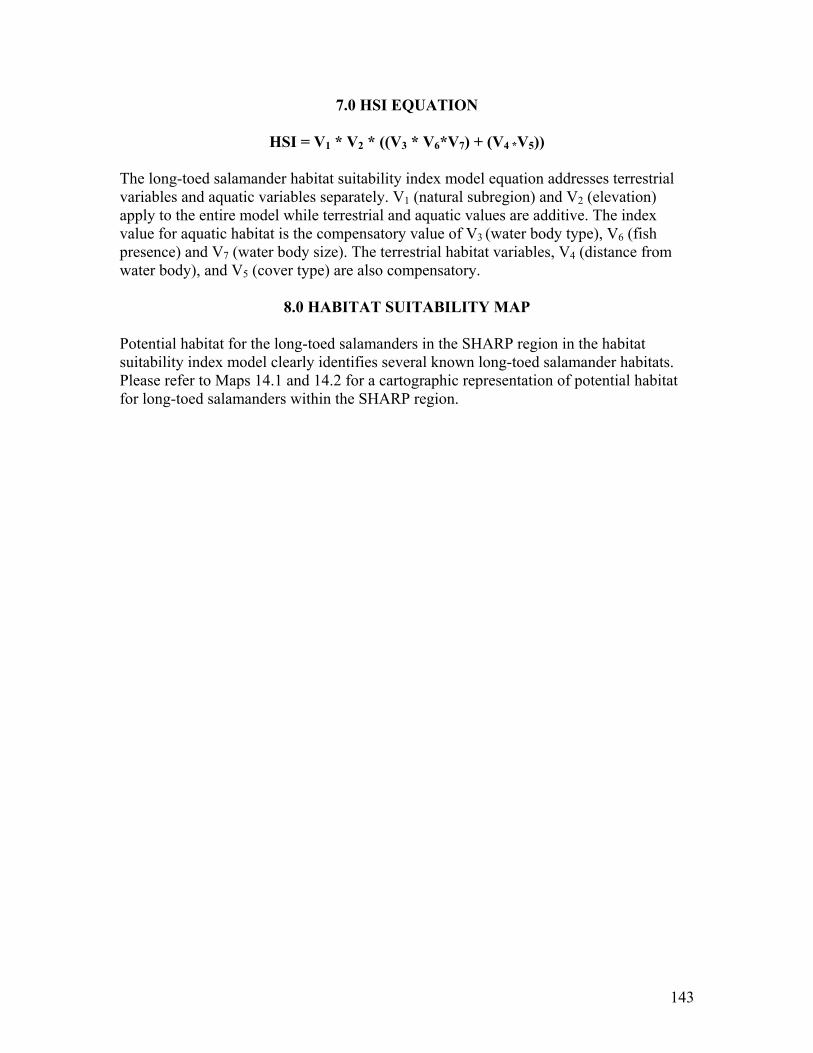
143
7.0 HSI EQUATION
HSI = V1 * V2 * ((V3 * V6*V7) + (V4 *V5)) The long-toed salamander habitat suitability index model equation addresses terrestrial variables and aquatic variables separately. V1 (natural subregion) and V2 (elevation) apply to the entire model while terrestrial and aquatic values are additive. The index value for aquatic habitat is the compensatory value of V3 (water body type), V6 (fish presence) and V7 (water body size). The terrestrial habitat variables, V4 (distance from water body), and V5 (cover type) are also compensatory.
8.0 HABITAT SUITABILITY MAP Potential habitat for the long-toed salamanders in the SHARP region in the habitat suitability index model clearly identifies several known long-toed salamander habitats. Please refer to Maps 14.1 and 14.2 for a cartographic representation of potential habitat for long-toed salamanders within the SHARP region.
144
9.0 LITERATURE CITED Alberta Sustainable Resource Development. 2000. The general status of Alberta wild
species 2000. Alberta Sustainable Resource Development, Fish and Wildlife Service, Edmonton, AB. 46 pp.
Blaustein, A.R., D. G. Hokit, R.K.O�Hara, and R.A. Holt. 1994. Pathogenic fungus
contributes to amphibian losses in the Pacific Northwest. Biological Conservation 67: 251-254.
COSEWIC, 2003. Canadian species at risk, May 2003. Committee on the Status of Endangered Wildlife in Canada, Ottawa, ON. 43 pp.
Fukumoto, J. 1995. Long-toed salamander (Ambystoma macrodactylum) ecology and management in Waterton Lakes National Park. M.Env.D. Thesis. University of Calgary, Calgary, AB. 108 pp.
Funk, W.C. and W.W. Dunlap. 1999. Colonization of high-elevation lakes by long-toed
salamanders (Ambystoma macrodactylum) after the extinction of introduced trout populations. Can. J. Zool. 77: 1759-1767.
Graham, K.L. 1997. Habitat use by long-toed salamanders (Ambystoma macrodactylum)
at three different scales. M.Sc. Thesis. University of Guelph, Guelph, ON. Graham, K.L. and G.L. Powell. 1999. Status of the long-toed salamander (Ambystoma
macrodactylum) in Alberta. Alberta Environmental Protection, Fisheries and Wildlife Management Division, and Alberta Conservation Association, Alberta Wildlife Status Report No. 22, Edmonton, AB. 19 pp.
Kiesecker, J.M., A.R. Blaustein and C.L. Miller. 2001. Transfer of a pathogen from fish to amphibians. Conservation Biology 15:1064-1070.
Liss, W.J., G.L. Larson, E. Deimling, L. Ganio, R. Gresswell, R. Hoffman, M. Kiss, G.
Lomnicky, C.D. McIntire, R. Truitt, and T. Tyler. 1995. Ecological effects of stocked fish in naturally fishless high mountain lakes, North Cascades National Park Service Complex, WA, U.S.A. Technical Report NPS/PNROSU/NRTR-95-03: National Park Service, Pacific Northwest Region, Seattle, WA. 285 pp.
Matthews, K.R., R.A. Knapp, and K.L. Pope. 2002. Garter snake distributions in high-
elevation aquatic ecosystems: is there a link with declining amphibian populations and non-native trout introductions? Journal of Herpetology 36: 16-22.
Pearson, K. 2003. Distribution and habitat associations of the long-toed salamander
(Ambystoma macrodactylum) in the Oldman River drainage. Alberta Sustainable Resource Development, Fish and Wildlife Division, Alberta Species at Risk Report No 75, Edmonton, AB. 25 pp.

145
Pilliod, D. S. and C.R. Peterson. 2001. Local and landscape effects of introduced trout on amphibians in historically fishless watersheds. Ecosystems 4: 322-333.
Powell, G.L., S.J. Nelson, and A.P. Russell. 1993. The Bow Valley long-toed salamander
population study: a preliminary report on the 1992 field season. Alberta Environmental Protection, Fish and Wildlife Service, Edmonton, AB. 124 pp.
Powell, G.L. and A.P. Russell. 1996. The long-toed salamander in the Bow Corridor: a
preliminary report. Alberta Environmental Protection, Fish and Wildlife Division, Edmonton, AB. 37 pp.
Russell, A.M. and A.M. Bauer. 1993. The Amphibians and Reptiles of Alberta.
University of Calgary Press, Calgary, AB and University of Alberta Press, Edmonton, AB. 264 pp.
Russell, A.P., G.L. Powell, and D.R. Hall. 1996. Growth and age in Alberta long-toed
salamanders (Ambystoma macrodactylum krausei): a comparison of two methods of estimation. Canadian Journal of Zoology 74: 397-412.
Sheppard, R.F. 1977. The ecology and home range movements of Ambystoma
macrodactylum krausei (Amphibia: Urodela). Master�s Thesis. University of Calgary, Department of Biology. Calgary, Alberta.
Tyler, T., W.J. Liss, L.M. Ganio, G.L. Larson, R. Hoffman, E. Deimling and G.
Lomnicky. 1998. Interaction between introduced trout and larval salamanders (Ambystoma macrodactylum) in high-elevation lakes. Conservation Biology 12: 94-105.
Wallis, C., C. Wershler, and R. Riddell. 2002. Ecological land classification of Waterton
Lakes National Park, Alberta. Vol. II: wildlife resources. Parks Canada, Waterton Park, AB 258 pp.
Wildy, E.L., D.P. Chivers, J.M. Kiesecker, and A.R. Blaustein. 2001. The effects of food
level and conspecific density on biting and cannibalism in larval long-toed salamanders, Ambystoma macrodactylum. Oecologia 128: 202-209.

146
Map 14. 1. Potential and known habitat for the long-toed salamander in the south end (south of Highway #3) of the SHARP area.

147
Map 14. 2. Potential and known habitat for the long-toed salamander in the north end (north of Highway #3) of the SHARP area.

148
Western Toad (Bufo boreas)
Kimberly J. Pearson Wildlife Consultant, Waterton, AB
1.0 PURPOSE AND LIMITATIONS
The purpose of this habitat suitability index (HSI) model is to indicate minimum potential habitat for western toad (Bufo boreas) within the Southern Headwaters at Risk Project (SHARP) area. As this is a landscape level model with coarse variables, it may not be directly applicable to other areas or to site-specific analysis. This model was constructed within the limitations of the spatial data available, primarily for management purposes. The model represents the minimum potential western toad habitat in the SHARP area. The western toad is a species with several microhabitat associations; unfortunately, it was not possible to include such microhabitat features in this model. This model is based on published and unpublished literature and expert opinion, and has not been field-tested.
2.0 GENERAL INFORMATION The western toad is distributed from southern Alaska to Baja California and as far east as Alberta and Colorado (Russell and Bauer 1993). Although wide ranging, its distribution is patchy (Davis 2002). Adult and juvenile western toads have wide bodies, short legs and dry, bumpy skin (Corkran and Thoms 1996). Adult toads usually have a thin, light-coloured stripe down the back (Corkran and Thoms 1996). Significant declines and extirpations of western toad have been documented in southern portions of the species� range and on Vancouver Island (Carey 1993; Davis 2000). The specific causes of such declines have not been positively identified to date, but research has suggested disease, fungal pathogens, habitat modification, susceptibility to UV radiation, predation and presence of introduced salmonids (Wind and Dupuis 2002; Davis 2000; Carey 1993). Declines in western toad have also been observed in Waterton Lakes National Park (WLNP), where breeding evidence has been absent at many sites where the toads bred as recently as 1994 (Wallis et al. 2002; Snyder et al. 2003). Western toads are designated as Sensitive in Alberta because their population trend in the province is unknown and because the species is declining in other parts of its range (Alberta Sustainable Resource Development 2000). COSEWIC (2003) considers the western toad a Species of Special Concern. Western toads reach sexual maturity at four to six years of age and can live to 11 years (Olson 1988, 1992 and Carey 1978 in Davis 2000). Western toad tadpoles congregate in masses of up to millions of individuals, which act as important converters of biomass and a tremendous prey source (Wind and Dupuis 2000; Davis 2002). Toads are generally most active at night but are thought to be more active diurnally at higher elevation habitats (Wind and Dupuis 2000).
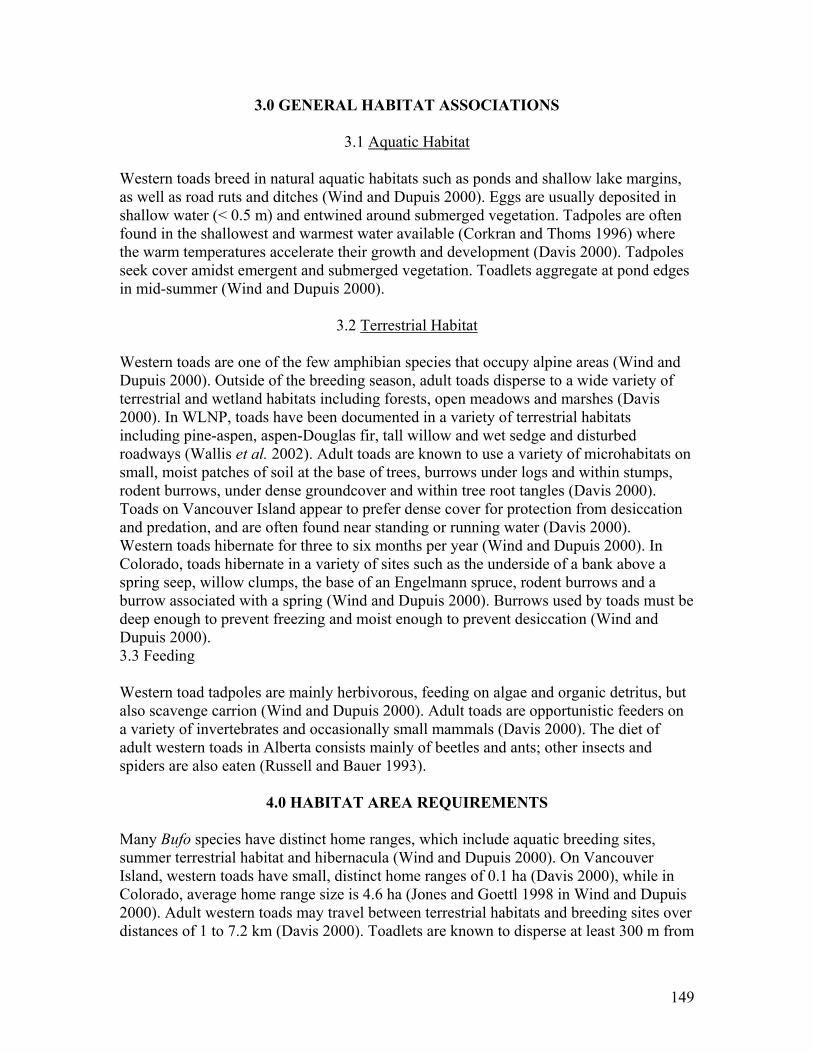
149
3.0 GENERAL HABITAT ASSOCIATIONS
3.1 Aquatic Habitat Western toads breed in natural aquatic habitats such as ponds and shallow lake margins, as well as road ruts and ditches (Wind and Dupuis 2000). Eggs are usually deposited in shallow water (< 0.5 m) and entwined around submerged vegetation. Tadpoles are often found in the shallowest and warmest water available (Corkran and Thoms 1996) where the warm temperatures accelerate their growth and development (Davis 2000). Tadpoles seek cover amidst emergent and submerged vegetation. Toadlets aggregate at pond edges in mid-summer (Wind and Dupuis 2000).
3.2 Terrestrial Habitat
Western toads are one of the few amphibian species that occupy alpine areas (Wind and Dupuis 2000). Outside of the breeding season, adult toads disperse to a wide variety of terrestrial and wetland habitats including forests, open meadows and marshes (Davis 2000). In WLNP, toads have been documented in a variety of terrestrial habitats including pine-aspen, aspen-Douglas fir, tall willow and wet sedge and disturbed roadways (Wallis et al. 2002). Adult toads are known to use a variety of microhabitats on small, moist patches of soil at the base of trees, burrows under logs and within stumps, rodent burrows, under dense groundcover and within tree root tangles (Davis 2000). Toads on Vancouver Island appear to prefer dense cover for protection from desiccation and predation, and are often found near standing or running water (Davis 2000). Western toads hibernate for three to six months per year (Wind and Dupuis 2000). In Colorado, toads hibernate in a variety of sites such as the underside of a bank above a spring seep, willow clumps, the base of an Engelmann spruce, rodent burrows and a burrow associated with a spring (Wind and Dupuis 2000). Burrows used by toads must be deep enough to prevent freezing and moist enough to prevent desiccation (Wind and Dupuis 2000). 3.3 Feeding Western toad tadpoles are mainly herbivorous, feeding on algae and organic detritus, but also scavenge carrion (Wind and Dupuis 2000). Adult toads are opportunistic feeders on a variety of invertebrates and occasionally small mammals (Davis 2000). The diet of adult western toads in Alberta consists mainly of beetles and ants; other insects and spiders are also eaten (Russell and Bauer 1993).
4.0 HABITAT AREA REQUIREMENTS Many Bufo species have distinct home ranges, which include aquatic breeding sites, summer terrestrial habitat and hibernacula (Wind and Dupuis 2000). On Vancouver Island, western toads have small, distinct home ranges of 0.1 ha (Davis 2000), while in Colorado, average home range size is 4.6 ha (Jones and Goettl 1998 in Wind and Dupuis 2000). Adult western toads may travel between terrestrial habitats and breeding sites over distances of 1 to 7.2 km (Davis 2000). Toadlets are known to disperse at least 300 m from

150
natal ponds into terrestrial and wetland habitats (Davis 2000). Home range, microsite and breeding site fidelity is common in western toads; displaced individuals have returned to their original locations from up to 1 km away (Wind and Dupuis 2000; Davis 2000).
5.0 ASSOCIATED SPECIES The habitats and ranges of long-toed salamander (Ambystoma macrodactylum), tiger salamander (Ambystoma tigrinum), striped chorus frog (Pseudacris maculata), northern leopard frog (Rana pipiens) and Columbia spotted frog (Rana luteiventris) overlap to various extents with those of western toad in the SHARP area (Russell and Bauer 1993). As amphibian predators, garter snakes (Thamnophis spp.) are associated with areas of high amphibian density (Matthews et al. 2002) and thus with western toads, especially toadlets (Davis 2000). Toadlets are also prey to spotted sandpipers and American robins (Jones et al. 1999). Despite their toxic skin secretions, adults are eaten by snakes, owls, corvids, shrikes, gulls, weasels, skunks, bears, foxes and coyotes (Russell and Bauer 1993). Tadpoles contain a toxic pigment which deters predation by fish, but are prey to various vertebrates such as mallard ducks, herons, corvids and garter snakes, as well as invertebrates such as backswimmers and giant water bugs (Davis 2000; Wind and Dupuis 2000).
6.0 THE HSI MODEL
6.1 Selected Habitat Variables
6.1.1 Natural Subregion (V1)
Western toads are found mainly in the parkland, montane and subalpine regions of the SHARP area (Wallis et al. 2002; Snyder et al. 2003) (Figure 15.1). They are known to utilize alpine areas; however few suitable breeding habitats exist there. Toads occur less frequently in the fescue region (Russell and Bauer 1993), however that region was not represented in the model due to technical restrictions.
0
0.2
0.4
0.6
0.8
1
Parland Montane Subalpine Alpine OtherNatural Subregion
Suita
bilit
y In
dex
Figure 15. 1. Habitat suitability index for natural subregion (V1) for the western toad.
6.1.2 Water body Type (V2)
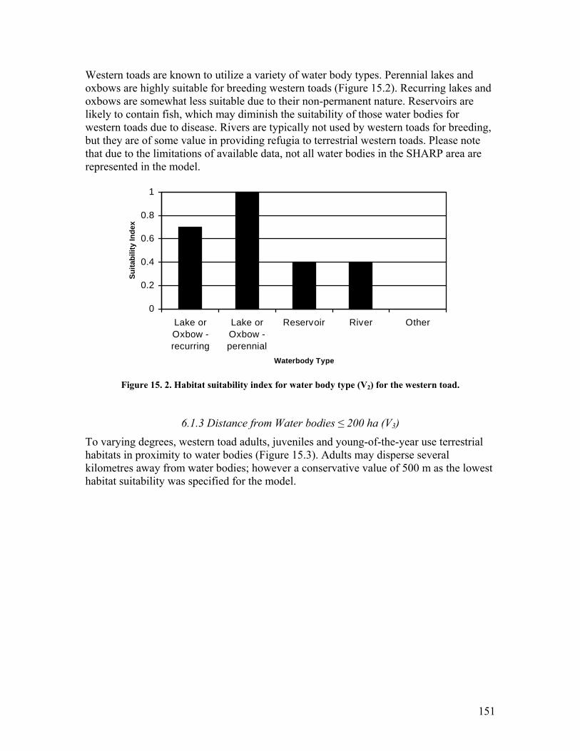
151
Western toads are known to utilize a variety of water body types. Perennial lakes and oxbows are highly suitable for breeding western toads (Figure 15.2). Recurring lakes and oxbows are somewhat less suitable due to their non-permanent nature. Reservoirs are likely to contain fish, which may diminish the suitability of those water bodies for western toads due to disease. Rivers are typically not used by western toads for breeding, but they are of some value in providing refugia to terrestrial western toads. Please note that due to the limitations of available data, not all water bodies in the SHARP area are represented in the model.
0
0.2
0.4
0.6
0.8
1
Lake orOxbow -recurring
Lake orOxbow -perennial
Reservoir River Other
Waterbody Type
Suita
bilit
y In
dex
Figure 15. 2. Habitat suitability index for water body type (V2) for the western toad.
6.1.3 Distance from Water bodies ≤ 200 ha (V3)
To varying degrees, western toad adults, juveniles and young-of-the-year use terrestrial habitats in proximity to water bodies (Figure 15.3). Adults may disperse several kilometres away from water bodies; however a conservative value of 500 m as the lowest habitat suitability was specified for the model.

152
0
0.2
0.4
0.6
0.8
1
0 100 200 300 400 500Distance from Waterbody <= 200 ha (m)
Suita
bilit
y In
dex
Figure 15. 3. Habitat suitability index for distance from water bodies ≤ 200 ha (V3) for the western
toad.
6.1.4 Cover (V4)
Western toads prefer dense cover for protection from desiccation and predation (Davis 2000). Areas classified by the Alberta Vegetation Inventory (AVI; Nesby 1996) as 71 -100 % crown closure (density class = �D�) were therefore rated at the highest possible habitat suitability for western toad (Figure 15.4). Areas of 51 � 70 % crown closure (density class = �C�) were rated at moderately high suitability, while areas with 31 � 50 % closure (density class = �B�) and 6 � 30 % closure (density class = �A�) were given moderate and low suitability indices, respectively. Areas with 0 � 5 % crown closure are considered non-forested by the AVI. Non-forested land classified as �open shrub� (So) and �closed shrub� (Sc) were considered suitable and given a suitability index value of �0.4� and �1� respectively. All other non-forested land and non-vegetated land categories were considered unsuitable.
0
0.2
0.4
0.6
0.8
1
A B C D Sc So OtherCover Class
Suita
bilit
y In
dex
Figure 15. 4. Habitat suitability index for cover (V4) for the western toad.
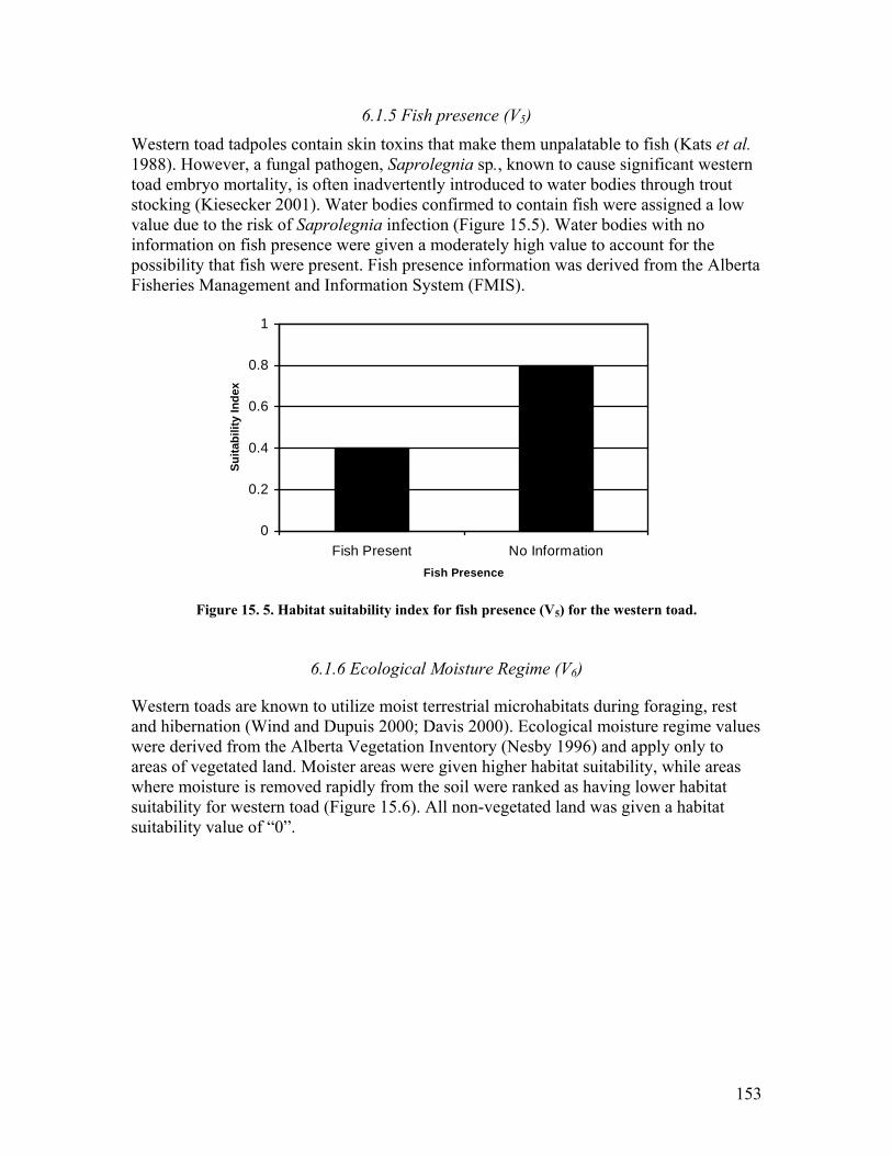
153
6.1.5 Fish presence (V5)
Western toad tadpoles contain skin toxins that make them unpalatable to fish (Kats et al. 1988). However, a fungal pathogen, Saprolegnia sp., known to cause significant western toad embryo mortality, is often inadvertently introduced to water bodies through trout stocking (Kiesecker 2001). Water bodies confirmed to contain fish were assigned a low value due to the risk of Saprolegnia infection (Figure 15.5). Water bodies with no information on fish presence were given a moderately high value to account for the possibility that fish were present. Fish presence information was derived from the Alberta Fisheries Management and Information System (FMIS).
0
0.2
0.4
0.6
0.8
1
Fish Present No InformationFish Presence
Suita
bilit
y In
dex
Figure 15. 5. Habitat suitability index for fish presence (V5) for the western toad.
6.1.6 Ecological Moisture Regime (V6)
Western toads are known to utilize moist terrestrial microhabitats during foraging, rest and hibernation (Wind and Dupuis 2000; Davis 2000). Ecological moisture regime values were derived from the Alberta Vegetation Inventory (Nesby 1996) and apply only to areas of vegetated land. Moister areas were given higher habitat suitability, while areas where moisture is removed rapidly from the soil were ranked as having lower habitat suitability for western toad (Figure 15.6). All non-vegetated land was given a habitat suitability value of �0�.

154
0
0.2
0.4
0.6
0.8
1
d (xeric) m (subhygric,mesic,
submesic)
w (hygric,subhygric)
a (hydric) Non-vegetated
landEcological Moisture Regime
Suita
bilit
y In
dex
Figure 15. 6. Habitat suitability index for ecological moisture regime (V6) for the western toad.
6.1.7. Distance from Water bodies > 200 ha (V7)
Because water bodies > 200 ha in size are of less suitability for breeding to western toads (see Section 6.1.8), toads are assumed to spend less time at and around those water bodies. Therefore, a higher rate of suitability index decrease with distance from those water bodies to 200 m was specified (Figure 15.7).
0
0.2
0.4
0.6
0.8
1
0 50 100 150 200Distance from Waterbody > 200 ha (m)
Suita
bilit
y In
dex
Figure 15. 7. Habitat suitability index for distance from water bodies > 200 ha (V7) for the western
toad.
6.1.8 Water body Size (V8)
Water bodies (excluding rivers) > 200 ha in area were considered to be of no habitat value to western toads (Figure 15.8). Western toads are less likely to breed successfully in larger water bodies because they are likely to contain fish, lack suitable egg-laying

155
substrates and/or are prone to disturbances such as motor boating and high winds. Water bodies ≤ 200 ha were assigned the highest habitat suitability.
0
0.2
0.4
0.6
0.8
1
<= 200 > 200Waterbody Size (ha)
Suita
bilit
y In
dex
Figure 15. 8. Habitat suitability index for water body size (V8) for the western toad.
7.0 HSI EQUATION
HSI = V1* [(Max (V3, V7) * (V4* V6)) + (V2 * V5 * V8)]
The western toad habitat suitability index model equation addresses both the terrestrial and the aquatic components of the habitat. Each component of the habitat is independent of the other. The index value for the aquatic component results from the full interaction of three variables. It is driven by V2 (water body type), and modified by V5 (fish presence) and V8 (water body size). If any variable of the aquatic habitat is �0�, then the aquatic component of the habitat is also �0� and unsuitable. The index value for the terrestrial component also results from the full interaction of three variables. It is driven by V4 (cover), and is modified by V6 (ecological moisture regime) and either V3 or V7 (distance from water body). Distance from water bodies is compensatory and takes the highest value between V3 (distance from water body ≤ 200 ha) and V7 (distance from water body > 200 ha). Here again, a �0� value for any of the terrestrial variables will result in a non-suitable terrestrial component of the habitat. V1 (natural subregion) is a landscape variable that applies at a higher ecological scale and modifies all the habitat components.

156
7.0 HABITAT SUITABILITY MAP The habitat suitability maps for the western toad identify potential habitat in the SHARP region (Maps 15.1 and 15.2).
8.0 LITERATURE CITED Alberta Sustainable Resource Development. 2000. The general status of Alberta wild
species 2000. Alberta Sustainable Resource Development, Fish and Wildlife Service, Edmonton, AB. 46 pp.
Carey, C. 1993. Hypothesis concerning the causes of the disappearance of boreal toads
from the mountains of Colorado. Conservation Biology 7:355-362.
Corkran, C.C. and C. Thoms. 1996. Amphibians of Oregon, Washington, and British Columbia. A field identification guide. Lone Pine Publishing, Edmonton, Alberta, Canada. 175 pp.
COSEWIC, 2003. Canadian species at risk, May 2003. Committee on the Status of Endangered Wildlife in Canada, Ottawa, ON. 43 pp.
Davis, T.M. 2000. Ecology of the western toad (Bufo boreas) in forested areas on Vancouver Island, final report. Forest Renewal B.C., Ministry of Forests, Victoria, B.C. 28 pp.
Davis, T.M. 2002. Research priorities for the management of the western toad, Bufo
boreas, in British Columbia. British Columbia Ministry of Water, Land and Air Protection, Biodiversity Branch, Victoria, BC. Wildlife Working Report No. WR-106. 35 pp.
Jones, M.S., J.P. Goettl, and L.J. Livo. 1999. Bufo boreas (Boreal toad). Predation.
Herpetological Review 30:91. Kats, L.B., J.W. Petranka, and A. Sih. 1988. Antipredator defenses and the persistence of
amphibian larvae with fishes. Ecology 69:1865-1870. Kiesecker, J.M., A.R. Blaustein and C.L. Miller. 2001. Transfer of a pathogen from fish
to amphibians. Conservation Biology 15:1064-1070.
Nesby, R. 1996. Alberta Vegetation Inventory Standards Manual v. 2.2. Alberta Environment Protection. Unpublished Document. 42 pp + appendices.
Russell, A.M. and A.M. Bauer. 1993. The Amphibians and Reptiles of Alberta.
University of Calgary Press, Calgary, AB and University of Alberta Press, Edmonton, AB. 264 pp.

157
Snyder, M., K.J. Pearson, and C.M. Smith. 2003. Waterton Lakes National Park
ecological monitoring program summary, 1997-2002. Unpublished Technical Report. Parks Canada, Waterton Park, AB. 78 pp.
Wallis, C., C. Wershler, and R. Riddell. 2002. Ecological land classification of Waterton Lakes National Park, Alberta. Vol. II: wildlife resources. Parks Canada, Waterton Park, AB 258 pp.
Wind, E. and L.A. Dupuis. 2002. COSEWIC Status Report on the Western Toad, Bufo
boreas, in Canada. Committee on the Status of Endangered Wildlife in Canada, Ottawa, ON. 81 pp.

158
Map 15. 1. Potential habitat for the western toad in the north end (north of Highway #3) of the SHARP area.

159
Map 15. 2. Potential habitat for the western toad in the south end (south of Highway #3) of the SHARP area.

160
Northern Leopard Frog (Rana pipiens)
Kimberly J. Pearson Wildlife Consultant, Waterton, AB
1.0 PURPOSE AND LIMITATIONS
The purpose of this habitat suitability index (HSI) model is to indicate minimum potential habitat for northern leopard frog (Rana pipiens) within the Southern Headwaters at Risk Project (SHARP) area. As this is a landscape level model with coarse variables, it may not be directly applicable to other areas or to site-specific analysis. This model was constructed within the limitations of the spatial data available, primarily for management purposes. The model represents the minimum potential northern leopard frog habitat in the SHARP area. The northern leopard frog is a species with several microhabitat associations; unfortunately, it was not possible to include such microhabitat features in this model. This model is based on published and unpublished literature and expert opinion, and has not been field-tested.
2.0 GENERAL INFORMATION Four leopard frog species range throughout North and Central America. The northern leopard frog is a relatively cold-adapted member of the leopard frog complex and is the only member of the complex found in Canada (Seburn and Seburn 1998; Russell and Bauer 1993). Adult and juvenile northern leopard frogs are characterized by obvious dark dorsal spots bordered by light coloured rings on the back, legs and sides, a white belly, and prominent, light-coloured dorsolateral folds (Kendell 2002; Seburn and Seburn 1998). Background colour ranges from green to brown or tan (Kendell 2002). The northern leopard frog was once widely-distributed throughout southern Alberta, but a marked decline of the species took place in that area, including protected areas, beginning in approximately 1978 (Russell and Bauer 1993). In spite of several intensive surveys that took place 1995 through 2003, few northern leopard frog breeding populations have been identified in the SHARP area or Waterton Lakes National Park (WLNP) (Alberta Sustainable Resource Development 2003; Taylor and Smith 2003). The precise cause(s) of the decline are thus far unknown, but may include wetland drainage, habitat degradation due to cattle grazing, pesticide use, drought, pollution, parasites or disease (Seburn and Seburn 1998). The northern leopard frog is listed as At Risk in Alberta due to its disappearance from most of its provincial range (Alberta Sustainable Resource Development 2000). Comparable but less extensive population declines have been observed throughout Canada (Alberta Sustainable Resource Development 2000). Prairie populations of the species have been assigned Species of Special Concern status by COSEWIC (2003).

161
Northern leopard frogs become sexually mature at two or three years of age (Russell and Bauer 1993). Estimates of survival from embryo to metamorphosis ranged from one to six percent in Wisconsin (Hine et al. 1981). Timing and duration of breeding activities are temperature dependent (Alberta Sustainable Resource Development 2003).
3.0 GENERAL HABITAT ASSOCIATIONS
3.1 Aquatic Habitat For breeding, northern leopard frogs require non-acidic, shallow and warm, standing water at the edges of beaverponds, quiet backwaters, oxbows, springs, marshes, lakes, dugouts, ditches or borrow pits, preferably those with dense aquatic and emergent vegetation (Alberta Sustainable Resource Development 2003; Corkran and Thoms 1996; Russell and Bauer 1993). Aquatic vegetation species observed at Albertan northern leopard frog breeding sites include cattails, bulrushes and sedges (Wershler 1991). Eggs are attached to submerged vegetation in water 30 to 75 cm deep (Kendell 2002). Water at breeding sites is typically not silty and breeding pond substrates tend to be overlain with decomposing vegetation (Seburn and Seburn 1998). Aquatic habitats that do not contain fish and that contain water until at least late July or August are most suitable for breeding (Alberta Sustainable Resource Development 2003). In late fall and winter, northern leopard frogs hibernate in the muddy bottoms of standing water bodies or under rocks in streams and springs (Russell and Bauer 1993). Standing water bodies that do not freeze solid, are well-oxygenated and are less than 4ûC are required for successful hibernation (Kendell 2002). Most northern leopard frog hibernating sites are associated with springs in southern Alberta (Wershler 1991) but other suitable water bodies may include creeks, rivers, ponds, lakes and oxbows (Kendell 2002). Overwintering may take place successfully in water bodies containing fish (Emery et al. 1972).
3.2 Terrestrial Habitat Juvenile and adult northern leopard frogs forage in a variety of habitats, including vegetated areas of ponds and vegetated areas adjacent to ponds (Corkran and Thoms 1996). Adult frogs may disperse to moist areas up to 2 km from water, especially in the summer or after rain, but, like young-of-the-year and juveniles, tend to remain close to water bodies which they use as refugia when threatened (Alberta Sustainable Resource Development 2003; Seburn and Seburn 1998; Russell and Bauer 1993). Northern leopard frogs are generally found in terrestrial areas with a good deal of vegetative ground cover, preferably 15 to 30 cm tall (Seburn and Seburn 1998; Russell and Bauer 1993). In Alberta, diverse summer habitats observed include shorelines with little or no vegetation, shorelines with abundant vegetation including grasses, sedges and willows, and open areas away from shorelines (Wershler 1991). In the Cypress Hills,

162
there was no difference found in the number of frogs that occupied wooded versus non-wooded habitats (Seburn 1994 in Alberta Sustainable Resource Development 2003).
3.3 Feeding Terrestrial northern leopard frogs are known to feed mainly on insects and to a lesser extent on arachnids, earthworms, snails and slugs (Moore and Strickland 1954). The majority of the insect diet is comprised of beetles, flies, grasshoppers and crickets (Moore and Strickland 1954). Northern leopard frogs are also known to prey opportunistically on birds, garter snakes, tadpoles, frogs and fish of appropriate sizes (Russell and Bauer 1993). Frogs feed during both the day and night (Seburn and Seburn 1998). Northern leopard frog larvae are primarily herbivorous, but they are known to feed on carrion, including dead toad tadpoles (Merrell 1977; Russell and Bauer 1993).
4.0 HABITAT AREA REQUIREMENTS Home ranges of adult northern leopard frogs in Michigan varied from 15 to 615 m2; subadult home ranges were 23 to 515 m2 (Dole 1965). Young-of-the-year northern leopard frogs travelled up to 2.1 km from their natal ponds through terrestrial and aquatic habitats in the Cypress Hills (Seburn et al. 1997). The proximity and connectedness of northern leopard frog breeding, hibernating and foraging habitats is of importance (Seburn et al. 1997). In Wisconsin, northern leopard frog breeding ponds were located within 1.6 km of suitable hibernating habitat (Hine et al. 1981). Overwintering and breeding have been observed in the same water body at some prairie sites (Seburn and Seburn 1998; Alberta Sustainable Resource Development 2003).
5.0 ASSOCIATED SPECIES
The general habitat associations and ranges of the following amphibians overlap to various extents with those of the northern leopard frog in the SHARP area: long-toed salamander (Ambystoma macrodactylum), tiger salamander (Ambystoma tigrinum), plains spadefoot toad (Spea bombifrons), western toad (Bufo boreas), striped chorus frog (Pseudacris maculata) and Columbia spotted frog (Rana luteiventris) (Russell and Bauer 1993). Adult and juvenile northern leopard frogs are common prey of garter snakes, small carnivores and birds (Russell and Bauer 1993). Tadpoles are preyed upon by waterfowl, fish and aquatic insects (Dickerson 1907).

163
6.0 THE HSI MODEL
6.1 Selected Habitat Variables
6.1.1 Natural Subregion (V1)
Current and historic distribution data for northern leopard frog in the SHARP region include the fescue, mixed grassland and foothills parkland natural regions (Figure 16.1) (Alberta Sustainable Resource Development 2003; Russell and Bauer 1993; Wallis et al. 2002). A few historic records of northern leopard frogs in the montane region also exist, though that region is considered less suitable for leopard frogs. Subalpine and alpine regions are not suitable for northern leopard frogs and are not included in the model.
0
0.2
0.4
0.6
0.8
1
FoothillsFescue
Mixedgrass FoothillsParkland
Montane Other
Natural Subregion
Suita
bilit
y In
dex
Figure 16. 1. Habitat suitability index for natural subregion (V1) for the northern leopard frog.
6.1.2 Water body Type (V2)
Perennial lakes and oxbows represent breeding and overwintering habitats of highest suitability to northern leopard frogs due to their potential to retain sufficient water for metamorphosis and overwintering (Figure 16.2). Recurring lakes and oxbows may not contain sufficient water to permit metamorphosis or overwintering but represent breeding habitat of moderate value. Canals, major canals and rivers tend to contain fish and fast-moving water, factors which limit breeding by northern leopard frogs, however those water bodies represent suitable overwintering habitats. Perennial streams provide moderate overwintering opportunities. Dugouts may provide suitable breeding habitats but are likely associated with disturbances by cattle, which may negatively affect breeding. Reservoirs are likely to contain fish so provide low quality breeding habitat but may be of value to overwintering northern leopard frogs. Please note that due to the limitations of available data, not all water bodies in the SHARP area are represented in the model.
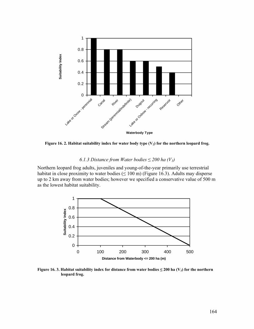
164
0
0.2
0.4
0.6
0.8
1
Lake
or O
xow - p
erenn
ial
Canal
River
Stream
(pere
nnial
/inde
finite
)
Dugou
t
Lake
or O
xbow
- rec
urring
Reserv
oirOthe
r
Waterbody Type
Suita
bilit
y In
dex
Figure 16. 2. Habitat suitability index for water body type (V2) for the northern leopard frog.
6.1.3 Distance from Water bodies ≤ 200 ha (V3)
Northern leopard frog adults, juveniles and young-of-the-year primarily use terrestrial habitat in close proximity to water bodies (≤ 100 m) (Figure 16.3). Adults may disperse up to 2 km away from water bodies; however we specified a conservative value of 500 m as the lowest habitat suitability.
0
0.2
0.4
0.6
0.8
1
0 100 200 300 400 500Distance from Waterbody <= 200 ha (m)
Suita
bilit
y In
dex
Figure 16. 3. Habitat suitability index for distance from water bodies ≤ 200 ha (V3) for the northern
leopard frog.

165
6.1.4 Distance from Water bodies > 200 ha (V4)
As in V3, northern leopard frog adults, juveniles and young-of-the-year use terrestrial habitat in close proximity (100 m) to water bodies. Because water bodies > 200 ha are of less suitability for breeding to northern leopard frogs (see Section 6.1.6), frogs are assumed to spend less time at and around those water bodies. Thus, we specified a higher rate of suitability index decrease with distance from those water bodies to 200 m (Figure 16.4).
0
0.2
0.4
0.6
0.8
1
0 50 100 150 200Distance from Waterbody > 200 ha (m)
Suita
bilit
y In
dex
Figure 16. 4. Habitat suitability index for distance from water bodies > 200 ha (V4) for the northern
leopard frog.
6.1.5 Presence of Fish (V5)
Fish presence information was derived from the Alberta Fisheries Management and Information System (FMIS). Trout have been observed to prey directly upon amphibian larvae and other species such as minnows can negatively affect the fitness and survival of larvae (Pearson 2003). A fungal pathogen, Saprolegnia, which can cause amphibian embryo mortality, may also be inadvertently introduced to water bodies through trout stocking (Kiesecker 2001; Blaustein et al. 1994). Water bodies confirmed to contain fish were assigned a very low value due to the risk of predation on frogs at all stages (Figure 5). Water bodies with no information on fish presence were assumed to not contain fish but were ranked moderately high to account for the possibility that fish were present.

166
0
0.2
0.4
0.6
0.8
1
Fish Present No InformationFish Presence
Suita
bilit
y In
dex
Figure 16. 5. Habitat suitability index for presence of fish (V5) for the northern leopard frog.
6.1.6 Water body Size (V6)
Water bodies less than or equal to 200 ha in size were considered of highest suitability to northern leopard frogs for breeding and overwintering (Figure 16.6). Larger water bodies in the SHARP area are more likely to contain fish, and generally provide less suitable breeding habitat to northern leopard frogs.
0
0.2
0.4
0.6
0.8
1
<= 200 >200Waterbody Size (ha)
Hab
itat S
uita
bilit
y
Figure 16. 6. Habitat suitability index for water body size (V6) for the northern leopard frog.

167
7.0 HSI EQUATION
HSI = V1 *[(V2 *V5*V6) + Max (V3 ,V4)] The northern leopard frog habitat suitability index model equation addresses both the terrestrial and the aquatic components of the habitat. Both components are independent. The terrestrial habitat component, distance from water bodies, is compensatory and takes the highest value between V3 (distance from water body ≤ 200 ha) and V4 (distance from water body > 200 ha). The aquatic habitat component results from the full interaction between the driving variable, V2 (water body type), and the modifying variables, V5 (presence of fish) and V6 (water body size). V1 (natural subregion) is of higher ecological scale and modifies both components of the habitat.
8.0 HABITAT SUITABILITY MAP Modeled potential habitat for the northern leopard frog in the SHARP region is presented on Maps 16.1 and 16.2.
9.0 LITERATURE CITED Alberta Sustainable Resource Development. 2000. The general status of Alberta wild
species 2000. Alberta Sustainable Resource Development, Fish and Wildlife Service, Edmonton, AB. 46 pp.
Alberta Sustainable Resource Development. 2003. Status of the northern leopard frog
(Rana pipiens) in Alberta: Update 2003. Alberta Sustainable Resource Development, Fish and Wildlife Division, and Alberta Conservation Association, Wildlife Status Report No. 9 (Update 2003), Edmonton, AB. 61 pp.
Blaustein, A.R., D. G. Hokit, R.K.O�Hara, and R.A. Holt. 1994. Pathogenic fungus
contributes to amphibian losses in the Pacific Northwest. Biological Conservation 67:251-254.
Corkran, C.C. and C. Thoms. 1996. Amphibians of Oregon, Washington, and British
Columbia. A field identification guide. Lone Pine Publishing, Edmonton, Alberta, Canada. 175 pp.
COSEWIC, 2003. Canadian species at risk, May 2003. Committee on the Status of Endangered Wildlife in Canada, Ottawa, ON. 43 pp.
Dickerson, M.C. 1097. The Frog Book: North American toads and frogs with a study of
the habits and life histories of those of the northeastern states. New York: Doubleday, Page & Co.

168
Dole, J.W. 1965. Summer movements of adult leopard frogs, Rana pipiens Schreber, in Northern Michigan. Ecology 46:236-255.
Emery, A.R., A.H. Berst, and K. Kodaira. 1972. Under-ice observations of wintering sites
of leopard frogs. Copeia 1972:123-126. Hine, R.L, B.L. Les and B.F. Hellmich. 1981. Leopard frog populations and mortality in
Wisconsin, 1974-1976. Technical Bulletin No. 122, Department of Natural Resources, Madison, WI. 39 pp.
Kendell, K. 2002. Survey protocol for the northern leopard frog. Alberta Sustainable
Resource Development, Fish and Wildlife Division, Alberta Species at Risk Report No. 43, Edmonton, AB. 30 pp.
Kiesecker, J.M., A.R. Blaustein and C.L. Miller. 2001. Transfer of a pathogen from fish
to amphibians. Conservation Biology 15:1064-1070. Merrell, D.J. 1977. Life History of the Leopard Frog, Rana pipiens, in Minnesota.
Minneapolis, Minnesota: Bell Museum of Natural History, University of Minnesota.
Moore, J.E. and E.H. Strickland. 1954. Notes on the food of Alberta amphibians.
American Midland Naturalist 52:221-224. Pearson, K. 2003. Distribution and habitat associations of the long-toed salamander
(Ambystoma macrodactylum) in the Oldman River drainage. Alberta Sustainable Resource Development, Fish and Wildlife Division, Alberta Species at Risk Report No 75, Edmonton, AB. 25 pp.
Russell, A.M. and A.M. Bauer. 1993. The Amphibians and Reptiles of Alberta.
University of Calgary Press, Calgary, AB and University of Alberta Press, Edmonton, AB. 264 pp.
Seburn, C.N.L., Seburn, D.C. and C.A. Paszkowski. 1997. Northern leopard frog (Rana
pipiens) dispersal in relation to habitat. In Amphibians in Decline: Canadian Studies of a Global Problem, D.M. Green, Ed. Herpetological Conservation. Society of the Study of Amphibians and Reptiles, St. Louis. 1:64-72.
Seburn, C.N.L. and D.C. Seburn. 1998. COSEWIC status report on the northern leopard
frog (Rana pipiens) in Canada (western populations). Seburn Ecological Services, Oxford Mills, ON. 41 pp.
Taylor, M., and C.M. Smith. 2003. Northern leopard frog and western toad inventory in
Waterton Lakes National Park, Alberta, in 2003. Unpublished Technical Report. Parks Canada, Waterton Park, AB. 83 pp.
169
Wallis, C., C. Wershler, and R. Riddell. 2002. Ecological land classification of Waterton Lakes National Park, Alberta. Vol. II: wildlife resources. Parks Canada, Waterton Park, AB. 258 pp.
Wershler, C. 1991. Status of the northern leopard frog in Alberta � 1990. Alberta Forestry
Lands and Wildlife. Edmonton, Alberta.
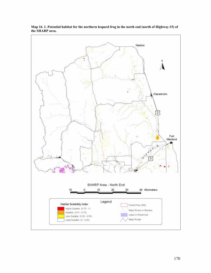
170
Map 16. 1. Potential habitat for the northern leopard frog in the north end (north of Highway #3) of the SHARP area.

171
Map 16. 2. Potential habitat for the northern leopard frog in the south end (south of Highway #3) of the SHARP area.

172
Appendix 1. Alberta Natural Heritage Information Centre�s ranking system (modified from Vujnovic and Gould (2002)). Elements (of biodiversity) are evaluated and ranked on their status (globally and state/provincially) using a system developed by The Nature Conservancy that is in use throughout North America. Ranking is usually based primarily on the number of occurrences, since that is frequently the only information available. Information, such as population size and trend, life history and reproductive strategies, range and current threats is used when available. Provincially, the ranks in Alberta are defined as: S1: < 5 occurrences or only a few remaining individuals. S2: 6-20 occurrences or with many individuals in fewer occurrences. S3: 21-100 occurrences may be rare and local throughout its range, or in a restricted range (may be abundant in some locations or may be vulnerable to extirpation because of some factor of its biology). S4: apparently secure under present conditions, typically >100 occurrences but may be fewer with many large populations; may be rare in parts of its range, especially peripherally. S5: demonstrably secure under present conditions, > 100 occurrences, may be rare in parts of its range, especially peripherally. SU: status uncertain often because of low search effort or cryptic nature of the element; possibly in peril, unrankable, more information needed. SH: historically known, may be relocated in the future. Other codes are: E: exotic species established, may be native to nearby regions HYB: hybrid taxon that is recurrent in the landscape P: potentially exists; may have occurred historically (but having not been persuasively documented) Q: taxonomic questions or problems R: reported but lacking sufficient documentation to accept or reject RD: report dubious RF: reported falsely T_: rank for a subspecific taxon X: believed to be extirpated S?: not yet ranked _?: rank questionable

173
Appendix 2. Focal species selection matrix (used as a guide in the final selection of SAR management species). Species in blue (and most of those in red) are those that scored high (arbitrarily set at >50). Those in red were chosen as focal species following evaluation of the final score. The rating given to each species-criterion varied between 0-2; (0- criterion does not apply for this species; 1- criterion applies to some extent for this species; 2- criterion applies to a great extent for this species). Each rating was averaged for all 10 expert reviewers, multiplied by the criterion weight, added to all scores for the species, and weighed for the final score out of 100. The �#Raters� is a reflection of the number of reviewers that rated the species. Reviewers were not required to fill out every species-criterion combinations.

174
Appendix 3. Species at risk, may be at risk, or data deficient in the SHARP area.
Species Name Common Name AB Gen. Status1 / COSEWIC Status
Designation AB Wildlife Act
Reference (range)
Mammals: Gulo gulo Wolverine May Be At Risk /
Special Concern Fur-Bearing Animal (Data Deficient)
Petersen (1997).
Felis concolor Mountain Lion/ Cougar
Sensitive / N/A Big Game Smith (1993).
Lemmiscus curtatus Sagebrush Vole Secure / Data Deficient N/A Smith (1993). Lynx canadensis Canada Lynx Sensitive / Not at Risk Fur-Bearing Animal
(Felis lynx) Smith (1993).
Lynx rufus Bobcat Sensitive / N/A Fur-Bearing Animal (Felis rufus)
Smith (1993).
Microtus richardsoni Water Vole Sensitive / N/A Non-Game Animal Rintoul (2003). Mustela frenata Long-Tailed
Weasel May Be At Risk / Not at Risk
Fur-Bearing Animal Smith (1993).
Myotis volans Long-legged Myotis
Undetermined / N/A Non-license Animal Smith (1993).
Sorex vagrans Vagrant Shrew May Be At Risk / N/A Controlled Animals Rintoul (2003). Spermophilus columbianus
Columbian Ground Squirrel
Secure / N/A Non-license Animal Smith (1993).
Spermophilus tridecemlineatus
Thirteen-Lined Ground Squirrel
Undetermined / N/A Non-licence Animal Smith (1993).
Tamias ruficaudus Red-tailed Chipmunk
Sensitive / Candidate spp
Non-Game Animal Bennett (1999), Rintoul (2003).
Taxidea taxus American Badger Sensitive / N/A Fur-Bearing Animal Smith (1993). Ursus arctos Grizzly Bear May Be At Risk /
Special Concern Big Game Animal Kansas (2002).
Birds: Accipiter gentilis Northern
Goshawk Sensitive / Not at Risk Bird of Prey Gough et al.
(1998). Ammodramus bairdii Baird's Sparrow Sensitive / Not at Risk Non-Game Animal Gough et al.
(1998). Ammodramus savannarum
Grasshopper Sparrow
Sensitive / N/A Non-Game Animal Gough et al. (1998).
Anthus spragueii Sprague�s Pipit Sensitive / Threatened Non-Game Animal (Special Concern)
Prescott (1997).
Aquila chrysaetos Golden Eagle Sensitive / Not At Risk Bird of Prey Gough et al. (1998), Rintoul (2003).
Ardea herodias Great Blue Heron Sensitive / N/A Non-Game Animal Gough et al. (1998).
Asio flammeus Short-eared Owl May Be At Risk / Special Concern
Bird of Prey Clayton (2000).
Athene cunicularia Burrowing Owl At Risk / Endangered Threatened Rintoul (2003). Bartramia longicauda Upland Sandpiper Sensitive / N/A Non-Game Animal Dechant et al.
(2001). Buteo regalis Ferruginous
Hawk
At Risk / Special Concern
Threatened Schmutz (1999).
Buteo swainsoni Swainson's Hawk Sensitive / N/A Bird of Prey Gough et al. (1998).
Certhia americana Brown Creeper Undetermined / N/A Non-Game Animal Collister (1997).

175
Species Name Common Name AB Gen. Status1 / COSEWIC Status
Designation AB Wildlife Act
Reference (range)
Chlidonias niger Black Tern Sensitive / Not at Risk Non-Game Animal Gough et al. (1998).
Chordeiles minor Common Nighthawk
Sensitive / N/A Non-Game Animal Gough et al. (1998).
Cygnus buccinator Trumpeter Swan At Risk / Not at Risk Threatened James (2000). Dryocopus pileatus Pileated
Woodpecker Sensitive / N/A Non-Game Animal Gough et al.
(1998). Empidonax difficilis Cordilleran
Flycatcher Undetermined / N/A Non Game Semenchuk (1992).
Falco mexicanus Prairie Falcon Sensitive / Not at Risk Bird of Prey Paton (2002). Falco peregrinus Peregrine Falcon At Risk / Threatened Threatened Rintoul (2003). Glaucidium gnoma californicum
Northern Pygmy Owl
Sensitive / N/A Bird of Prey Hannah (1999).
Grus canadensis Sandhill Crane Sensitive / N/A Non-Game Animal Gough et al. (1998).
Haliaeetus leucocephalus
Bald Eagle Sensitive / Not at Risk Bird of Prey Gough et al. (1998).
Histrionicus histrionicus
Harlequin Duck Sensitive / N/A Migratory Game Bird
MacCallum (2001), Rintoul (2003).
Lanius ludovicianus Loggerhead Shrike
Sensitive / Threatened Non-Game Animal (Special Concern)
Prescott & Bjorge (1999).
Nycticorax nycticorax Black-crowned night-heron
Sensitive / N/A Non-Game Animal Gough et al. (1998).
Nucifraga columbiana Clark�s Nutcracker
Secure / N/A Non Game Semenchuk (1992).
Numenius americanus Long-billed Curlew
May be at Risk / Special Concern
Non-Game Animal (Special Concern)
Hill (1998).
Pandion haliaetus Osprey Sensitive / N/A Bird of Prey Gough et al. (1998).
Picoides arcticus Black-backed Woodpecker
Sensitive / N/A Non-Game Animal Sibley (2000).
Piranga ludoviciana Western Tanager Sensitive / N/A Non-Game Animal Gough et al. (1998).
Podiceps auritus Horned Grebe Sensitive / N/A Non-Game Animal Gough et al. (1998).
Podilymbus podiceps Pied-billed Grebe Sensitive / N/A Non-Game Animal Semenchuk (1992). Sphyrapicus nuchalis Red-naped
Sapsucker Undetermined / N/A Non-Game Animal Gough et al.
(1998). Spizella [ breweri] taverneii
Timberline Sparrow
Sensitive / N/A Non-Game Animal Semenchuk (1992).
Strix nebulosa Great Gray Owl Sensitive / Not at Risk Bird of Prey Semenchuk (1992). Tympanuchus phasianellus
Sharp-tailed Grouse
Sensitive / N/A Upland Game Bird Semenchuk (1992).
Amphibians: Ambystoma tigrinum Tiger Salamander
(paedogenic populations)
Secure / Not at Risk Non-Licence Animal
C. Goater, Pers. Comm.
Ambystoma macrodactylum
Long-toed Salamander
Sensitive / N/A Non-Game Animal (Special Concern)
Rintoul (2003).
Bufo boreas Western Toad Sensitive / Special Concern
Non-Licence Animal
Rana luteiventris Columbia Spotted Frog
Sensitive / Not at Risk Non-Game Animal (Rana pretiosa)
Rintoul (2003).
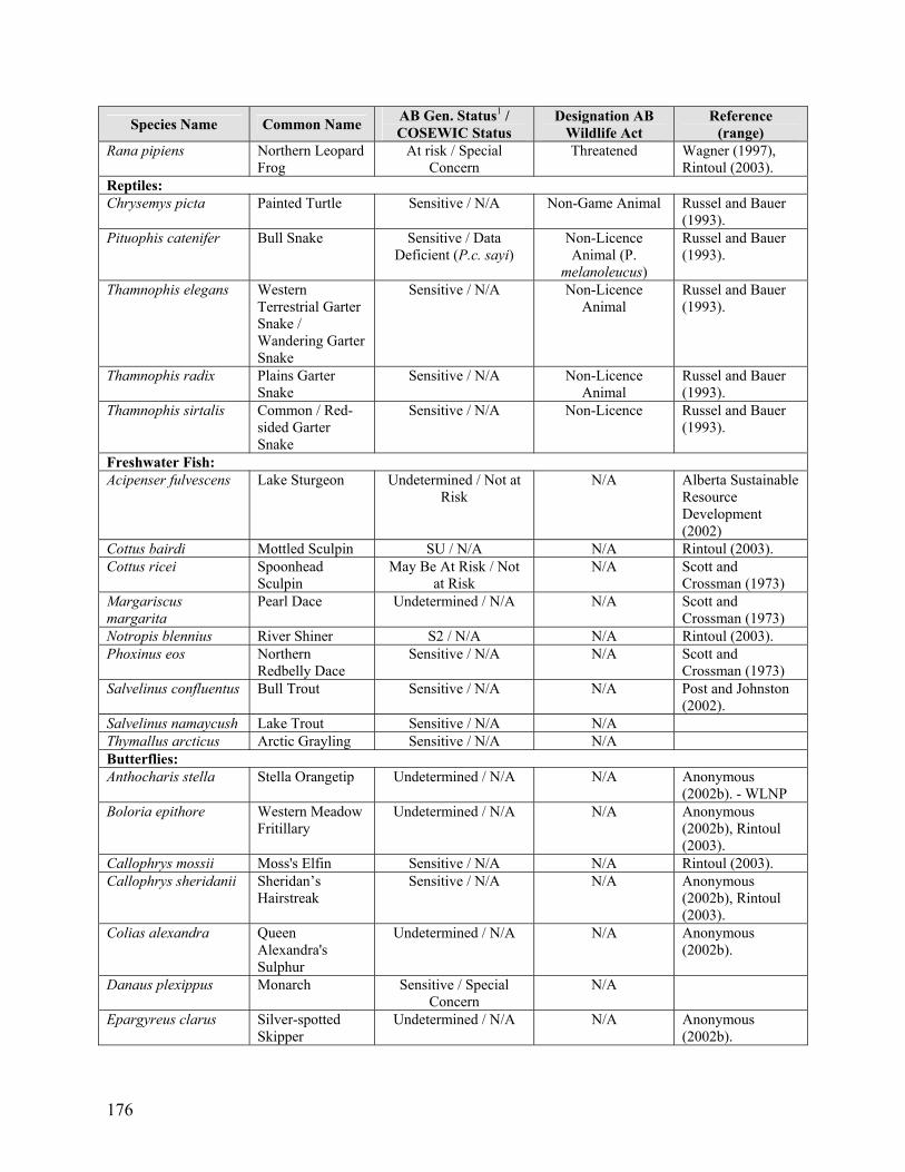
176
Species Name Common Name AB Gen. Status1 / COSEWIC Status
Designation AB Wildlife Act
Reference (range)
Rana pipiens Northern Leopard Frog
At risk / Special Concern
Threatened Wagner (1997), Rintoul (2003).
Reptiles: Chrysemys picta Painted Turtle Sensitive / N/A Non-Game Animal Russel and Bauer
(1993). Pituophis catenifer Bull Snake Sensitive / Data
Deficient (P.c. sayi) Non-Licence Animal (P.
melanoleucus)
Russel and Bauer (1993).
Thamnophis elegans Western Terrestrial Garter Snake / Wandering Garter Snake
Sensitive / N/A Non-Licence Animal
Russel and Bauer (1993).
Thamnophis radix Plains Garter Snake
Sensitive / N/A Non-Licence Animal
Russel and Bauer (1993).
Thamnophis sirtalis Common / Red-sided Garter Snake
Sensitive / N/A Non-Licence Russel and Bauer (1993).
Freshwater Fish: Acipenser fulvescens Lake Sturgeon Undetermined / Not at
Risk N/A Alberta Sustainable
Resource Development (2002)
Cottus bairdi Mottled Sculpin SU / N/A N/A Rintoul (2003). Cottus ricei Spoonhead
Sculpin May Be At Risk / Not
at Risk N/A Scott and
Crossman (1973) Margariscus margarita
Pearl Dace Undetermined / N/A N/A Scott and Crossman (1973)
Notropis blennius River Shiner S2 / N/A N/A Rintoul (2003). Phoxinus eos Northern
Redbelly Dace Sensitive / N/A N/A Scott and
Crossman (1973) Salvelinus confluentus Bull Trout Sensitive / N/A N/A Post and Johnston
(2002). Salvelinus namaycush Lake Trout Sensitive / N/A N/A Thymallus arcticus Arctic Grayling Sensitive / N/A N/A Butterflies: Anthocharis stella Stella Orangetip Undetermined / N/A N/A Anonymous
(2002b). - WLNP Boloria epithore Western Meadow
Fritillary Undetermined / N/A N/A Anonymous
(2002b), Rintoul (2003).
Callophrys mossii Moss's Elfin Sensitive / N/A N/A Rintoul (2003). Callophrys sheridanii Sheridan�s
Hairstreak Sensitive / N/A N/A Anonymous
(2002b), Rintoul (2003).
Colias alexandra Queen Alexandra's Sulphur
Undetermined / N/A N/A Anonymous (2002b).
Danaus plexippus Monarch Sensitive / Special Concern
N/A
Epargyreus clarus Silver-spotted Skipper
Undetermined / N/A N/A Anonymous (2002b).

177
Species Name Common Name AB Gen. Status1 / COSEWIC Status
Designation AB Wildlife Act
Reference (range)
Erynnis afranius Afranius Duskywing
Sensitive / N/A N/A Anonymous (2000b).
Euphydryas gillettii Gillette's Checkerspot
Sensitive / N/A N/A Anonymous (2002b).
Glaucopsyche piasus Glaucopsyche piasus
Sensitive / N/A N/A Anonymous (2002b).
Hesperia nevada Nevada Skipper Sensitive / N/A N/A Anonymous (2002b).
Hesperia uncas Uncas Skipper Sensitive / N/A N/A Anonymous (2002b).
Icaricia icarioides Boisduval's Blue Sensitive / N/A N/A Anonymous (2002b).
Icaricia shasta Shasta Blue Sensitive / N/A N/A Rintoul (2003). Ischnura cervula Pacific Forktail S2S3 / N/A N/A Rintoul (2003). Limenitis lorquini Lorquin's
Admiral Sensitive / N/A N/A Anonymous
(2002b), Rintoul (2003).
Lycaena dione Grey Copper Sensitive / N/A N/A Anonymous (2002b).
Lycaena heteronea Blue Copper Undetermined / N/A N/A Anonymous (2002b).
Neominois ridingsii Ridings' Satyr Sensitive / N/A N/A Anonymous (2002b).
Nymphalis californica California Tortoiseshell
Undetermined / N/A N/A Anonymous (2002b).
Ochlodes sylvanoides Woodland Skipper
Undetermined / N/A N/A Anonymous (2002b), Rintoul (2003).
Papilio eurymedon Pale Swallowtail Undetermined / N/A N/A Anonymous (2002b), Rintoul (2003).
Papilio machaon Old World Swallowtail
Sensitive / N/A N/A Anonymous (2002b).
Pieris oleracea Mustard White Undetermined / N/A N/A Anonymous (2002b).
Polites themistocles Tawny-edged Skipper
Undetermined / N/A N/A Anonymous (2002b).
Polygonia oreas Oreas Comma Undetermined / N/A N/A Anonymous (2002b).
Pyrgus ruralis Two-banded Checkered Skipper
Undetermined / N/A N/A Anonymous (2002b).
Satyrium acadicum Acadian Hairstreak
Undetermined / N/A N/A Rintoul (2003).
Sympetrum pallipes Striped Meadowhawk
S2S4 / N/A N/A Rintoul (2003).
Liverworts and Hornworts: Diplophyllum taxifolium
liverwort S1 / N/A N/A Rintoul (2003).
Jungermannia atrovirens
liverwort S2 / N/A N/A Rintoul (2003).
Jungermannia leiantha
liverwort S? / N/A N/A Rintoul (2003).

178
Species Name Common Name AB Gen. Status1 / COSEWIC Status
Designation AB Wildlife Act
Reference (range)
Jungermannia sphaerocarpa
liverwort S2 / N/A N/A Rintoul (2003).
Lophozia ascendens liverwort S2 / N/A N/A Rintoul (2003). Porella cordaeana liverwort S2 / N/A N/A Rintoul (2003). Porella platyphylla liverwort S1 / N/A N/A Rintoul (2003). Scapania curta liverwort S2 / N/A N/A Rintoul (2003). Scapania subalpina liverwort S2 / N/A N/A Rintoul (2003). Mosses: Anoectangium aestivum
S1 / N/A N/A Rintoul (2003).
Aulacomnium androgynum
S2 / N/A N/A Rintoul (2003).
Brachythecium frigidum
SU / N/A N/A Rintoul (2003).
Brachythecium hylotapetum
S2 / N/A N/A Rintoul (2003).
Brachythecium nelsonii
S2 / N/A N/A Rintoul (2003).
Brachythecium plumosum
S2 / N/A N/A Rintoul (2003).
Brachythecium reflexum
S1 / N/A N/A Rintoul (2003).
Bryum calobryoides S1 / N/A N/A Rintoul (2003). Cirriphyllum cirrosum S2 / N/A N/A Rintoul (2003). Coscinodon calyptratus
Sieve-toothed Big Calyptra Moss
S2 / N/A N/A Rintoul (2003).
Cynodontium strumiferum
S2S3 / N/A N/A Rintoul (2003).
Dicranella heteromalla
Silky Fork Moss S1 / N/A N/A Rintoul (2003).
Dicranum tauricum Broken-leaf Moss S1S2 / N/A N/A Rintoul (2003). Didymodon rigidulus Rigid Screw
Moss S2 / N/A N/A Rintoul (2003).
Didymodon vinealis S1 / N/A N/A Rintoul (2003). Drepanocladus crassicostatus
Brown Moss S2 / N/A N/A Rintoul (2003).
Encalypta brevicolla Candle-snuffer Moss
S2 / N/A N/A Rintoul (2003).
Encalypta spathulata Candle-snuffer Moss
S2 / N/A N/A Rintoul (2003).
Grimmia donniana Donian Grimmia S2 / N/A N/A Rintoul (2003). Grimmia montana Sun Grimmia S2 / N/A N/A Rintoul (2003). Grimmia alpestris Alpine Grimmia S2 / N/A N/A Rintoul (2003). Gymnostomum aeruginosum
Tufted Rock Beardless Moss
S2S3 / N/A N/A Rintoul (2003).
Homalothecium nevadense
S1 / N/A N/A Rintoul (2003).
Hygrohypnum bestii S2S3 / N/A N/A Rintoul (2003). Hygrohypnum styriacum
S1 / N/A N/A Rintoul (2003).
Jaffueliobryum wrightii
S2 / N/A N/A Rintoul (2003).

179
Species Name Common Name AB Gen. Status1 / COSEWIC Status
Designation AB Wildlife Act
Reference (range)
Leskeella nervosa S2 / N/A N/A Rintoul (2003). Mnium ambiguum S1S2 / N/A N/A Rintoul (2003). Orthotrichum affine SU / N/A N/A Rintoul (2003). Orthotrichum pallens S2 / N/A N/A Rintoul (2003). Orthotrichum pumilum
S1S2 / N/A N/A Rintoul (2003).
Phascum vlassovii S1 / N/A N/A Rintoul (2003). Pogonatum urnigerum Urn-like
Pogonatum S2S3 / N/A N/A Rintoul (2003).
Pohlia atropurpurea S1 / N/A N/A Rintoul (2003). Pohlia longicolla S1 / N/A N/A Rintoul (2003). Polytrichum lyallii Hair Cap Moss S2 / N/A N/A Rintoul (2003). Pseudoleskea patens S2 / N/A N/A Rintoul (2003). Pseudoleskea stenophylla
S1S2 / N/A N/A Rintoul (2003).
Pterygoneurum subsessile
S1 / N/A N/A Rintoul (2003).
Racomitrium sudeticum
S1S2 / N/A N/A Rintoul (2003).
Rhizomnium magnifolium
S2 / N/A N/A Rintoul (2003).
Rhizomnium nudum S2 / N/A N/A Rintoul (2003). Scouleria aquatica S2 / N/A N/A Rintoul (2003). Schistidium pulvinatum
S1 / N/A N/A Rintoul (2003).
Seligeria campylopoda
S2 / N/A N/A Rintoul (2003).
Splachnum ampullaceum
Flagon-fruited Splachnum
S2 / N/A N/A Rintoul (2003).
Splachnum sphaericum
Globe-fruited Splachnum
S2 / N/A N/A Rintoul (2003).
Stegonia pilifera S2 / N/A N/A Rintoul (2003). Timmia norvegica S2 / N/A N/A Rintoul (2003). Lichens: Acarospora arenacea S2 / N/A N/A Rintoul (2003). Allantoparmelia alpicola
S2 / N/A N/A Rintoul (2003).
Aspicilia pergibbosa S1 / N/A N/A Rintoul (2003). Aspicilia sublapponica
S1 / N/A N/A Rintoul (2003).
Bacidia hegetschweileri
S1 / N/A N/A Rintoul (2003).
Baeomyces rufus S2 / N/A N/A Rintoul (2003). Bryoria simplicior Old Man's Beard S2S3 / N/A N/A Rintoul (2003). Caloplaca atroalba S1 / N/A N/A Rintoul (2003). Caloplaca chrysophthalma
S1 / N/A N/A Rintoul (2003).
Caloplaca citrina Powdery Jewel Lichen
S1 / N/A N/A Rintoul (2003).
Caloplaca flavovirescens
S2 / N/A N/A Rintoul (2003).
Catillaria globulosa S1 / N/A N/A Rintoul (2003).

180
Species Name Common Name AB Gen. Status1 / COSEWIC Status
Designation AB Wildlife Act
Reference (range)
Catillaria nigroclavata
S2 / N/A N/A Rintoul (2003).
Cetraria arenaria S1 / N/A N/A Rintoul (2003). Chaenotheca trichialis
S2 / N/A N/A Rintoul (2003).
Cladonia bacilliformis S2S3 / N/A N/A Rintoul (2003). Cladonia robbinsii S2S3 / N/A N/A Rintoul (2003). Collema flaccidum S1 / N/A N/A Rintoul (2003). Collema crispum S2 / N/A N/A Rintoul (2003). Cyphelium inquinans S2 / N/A N/A Rintoul (2003). Cyphelium notarisii S2 / N/A N/A Rintoul (2003). Dactylina madreporiformis
S2 / N/A N/A Rintoul (2003).
Dermatocarpon intestiniforme
S2 / N/A N/A Rintoul (2003).
Endocarpon pusillum S2 / N/A N/A Rintoul (2003). Endocarpon tortuosum
S2 / N/A N/A Rintoul (2003).
Flavopunctelia soredica
S2 / N/A N/A Rintoul (2003).
Lecanora hypoptoides S2 / N/A N/A Rintoul (2003). Lecanora meridionalis
S1 / N/A N/A Rintoul (2003).
Lecanora pringlei S1S2 / N/A N/A Rintoul (2003). Lecanora saligna S1 / N/A N/A Rintoul (2003). Lecidea lithophila S2 / N/A N/A Rintoul (2003). Lecidella patavina S1S2 / N/A N/A Rintoul (2003). Lecidoma demissum S1 / N/A N/A Rintoul (2003). Lepraria incana S2 / N/A N/A Rintoul (2003). Lepraria lobificans S1 / N/A N/A Rintoul (2003). Leptogium gelatinosum
S2 / N/A N/A Rintoul (2003).
Melanelia infumata S2S3 / N/A N/A Rintoul (2003). Melanelia subelegantula
S2 / N/A N/A Rintoul (2003).
Mycoblastus sanguinarius
S2 / N/A N/A Rintoul (2003).
Mycocalicium subtile S2 / N/A N/A Rintoul (2003). Nodobryoria subdivergens
Old Man's Beard S1 / N/A N/A Rintoul (2003).
Ochrolechia frigida S1 / N/A N/A Rintoul (2003). Peltigera cinnamomea S2 / N/A N/A Rintoul (2003). Phaeophyscia sciastra S2 / N/A N/A Rintoul (2003). Phaeorrhiza sareptana
S1 / N/A N/A Rintoul (2003).
Phaeospora parasitica
S1 / N/A N/A Rintoul (2003).
Placidium lachneum S2? / N/A N/A Rintoul (2003). Placynthium asperellum
S1 / N/A N/A Rintoul (2003).
Psora globifera S1S2 / N/A N/A Rintoul (2003). Psora himalayana S2 / N/A N/A Rintoul (2003).

181
Species Name Common Name AB Gen. Status1 / COSEWIC Status
Designation AB Wildlife Act
Reference (range)
Psora nipponica S2 / N/A N/A Rintoul (2003). Psora tuckermanii S2 / N/A N/A Rintoul (2003). Pyrrhospora elabens S1 / N/A N/A Rintoul (2003). Rhizocarpon badioatrum
S1 / N/A N/A Rintoul (2003).
Rhizocarpon pusillum S1 / N/A N/A Rintoul (2003). Rhizocarpon superficiale
S2 / N/A N/A Rintoul (2003).
Rhizocarpon umbilicatum
S1 / N/A N/A Rintoul (2003).
Rinodina colobina S1 / N/A N/A Rintoul (2003). Rinodina mucronatula S1 / N/A N/A Rintoul (2003). Sarcogyne privigna S1 / N/A N/A Rintoul (2003). Tephromela atra Black-eye Lichen S2 / N/A N/A Rintoul (2003). Umbilicaria americana
S2 / N/A N/A Rintoul (2003).
Umbilicaria angulata S1S2 / N/A N/A Rintoul (2003). Verrucaria glaucovirens
S2 / N/A N/A Rintoul (2003).
Xanthoria fulva S1 / N/A N/A Rintoul (2003). Vascular Plants: Adenocaulon bicolor Pathfinder S2S3 / N/A N/A Rintoul (2003). Adiantum aleuticum Western
Maidenhair Fern May Be At Risk / N/A N/A Rintoul (2003).
Agrostis exarata Spike Redtop S2 / N/A N/A Rintoul (2003). Allium geyeri Geyer's Onion S2 / N/A N/A Rintoul (2003). Alopecurus alpinus Alpine Foxtail S2 / N/A N/A Rintoul (2003). Amaranthus californicus
Californian Amaranth
S1 / N/A N/A Rintoul (2003).
Antennaria aromatica Scented Everlasting
S2 / N/A N/A Rintoul (2003).
Antennaria corymbosa
Corymbose Everlasting
S1 / N/A N/A Rintoul (2003).
Antennaria luzuloides Silvery Everlasting
S1 / N/A N/A Rintoul (2003).
Aquilegia jonesii Jones' Columbine S2 / N/A N/A Rintoul (2003). Arabis lemmonii Lemmon's Rock
Cress S2 / N/A N/A Rintoul (2003).
Arnica amplexicaulis Stem-clasping Arnica
S2 / N/A N/A Rintoul (2003).
Arnica longifolia Long-leaved Arnica
S2 / N/A N/A Rintoul (2003).
Artemisia tridentata Big Sagebrush S2 / N/A N/A Rintoul (2003). Aster campestris Meadow Aster S2 / N/A N/A Rintoul (2003). Aster eatonii Eaton's Aster S2 / N/A N/A Rintoul (2003). Atriplex canescens Saltbush SU / N/A N/A Rintoul (2003). Barbarea orthoceras American Winter
Cress S2 / N/A N/A Rintoul (2003).
Botrychium ascendens Ascending Grape Fern
May Be At Risk / N/A N/A Rintoul (2003).
Botrychium campestre Field Grape Fern May Be At Risk / N/A N/A Rintoul (2003).

182
Species Name Common Name AB Gen. Status1 / COSEWIC Status
Designation AB Wildlife Act
Reference (range)
Botrychium hesperium Western Grape Fern
May Be At Risk / N/A N/A Rintoul (2003).
Botrychium lanceolatum
Lance-leaved Grape Fern
May Be At Risk / N/A N/A Rintoul (2003).
Botrychium lineare Straight-leaf Moonwort
S1 / N/A N/A Rintoul (2003).
Botrychium michiganense
SU / N/A N/A Rintoul (2003).
Botrychium minganense
Mingan Grape Fern
May Be At Risk / N/A N/A Rintoul (2003).
Botrychium pinnatum May Be At Risk / N/A N/A Rintoul (2003). Botrychium spathulatum
May Be At Risk / N/A N/A Rintoul (2003).
Brickellia grandiflora Large-flowered Brickellia
S2 / Not at Risk N/A Rintoul (2003).
Bromus latiglumis Canada Brome S1 / N/A N/A Rintoul (2003). Bromus vulgaris Woodland Brome S2S3 / N/A N/A Rintoul (2003). Calylophus serrulatus Shrubby Evening-
primrose S2 / N/A N/A Rintoul (2003).
Camassia quamash var quamash
Blue Camas S2 / N/A N/A Rintoul (2003).
Cardamine oligosperma var kamtschatica
Mountain Cress S2 / N/A N/A Rintoul (2003).
Carex mertensii Purple Sedge S1 / N/A N/A Rintoul (2003). Carex petasata Pasture Sedge S1S2 / N/A N/A Rintoul (2003). Carex platylepis Broad-Scaled
Sedge S1S2 / N/A N/A Rintoul (2003).
Carex preslii Presl Sedge S2 / N/A N/A Rintoul (2003). Carex scoparia Broom Sedge S1 / N/A N/A Rintoul (2003). Carex vesicaria Blister Sedge S1 / N/A N/A Rintoul (2003). Castilleja cusickii Yellow
Paintbrush S2S3 / N/A N/A Rintoul (2003).
Castilleja lutescens Stiff Yellow Paintbrush
S2S3 / N/A N/A Rintoul (2003).
Cirsium scariosum Thistle SU / N/A N/A Rintoul (2003). Conimitella williamsii Conimitella S2 / N/A N/A Rintoul (2003). Crepis atribarba Hawk's-beard S2 / N/A N/A Rintoul (2003). Crepis intermedia Intermediate
Hawk's-beard S2 / N/A N/A Rintoul (2003).
Cryptogramma stelleri
Steller's Rock Brake
May Be At Risk / N/A N/A Rintoul (2003).
Cypripedium montanum
Mountain Lady's-slipper
May Be At Risk / N/A N/A Rintoul (2003).
Deschampsia elongata
Slender Hair Grass
S1 / N/A N/A Rintoul (2003).
Downingia laeta Downingia S1S2 / N/A N/A Rintoul (2003). Draba densifolia Whitlow-grass S1S2 / N/A N/A Rintoul (2003). Draba longipes Whitlow-grass S1S2 / N/A N/A Rintoul (2003). Draba porsildii Porsild's
Whitlow-grass S2 / N/A N/A Rintoul (2003).
Ellisia nyctelea Waterpod S2 / N/A N/A Rintoul (2003).

183
Species Name Common Name AB Gen. Status1 / COSEWIC Status
Designation AB Wildlife Act
Reference (range)
Elymus scribneri Scribner's Wheat Grass
S2 / N/A N/A Rintoul (2003).
Elymus virginicus Virginia Wild Rye
S1 / N/A N/A Rintoul (2003).
Epilobium clavatum Willowherb S2 / N/A N/A Rintoul (2003). Epilobium glaberrimum ssp fastigiatum
Willowherb S1 / N/A N/A Rintoul (2003).
Epilobium lactiflorum Willowherb S2 / N/A N/A Rintoul (2003). Erigeron divergens Fleabane S1 / N/A N/A Rintoul (2003). Erigeron flagellaris Creeping
Fleabane S1 / N/A N/A Rintoul (2003).
Erigeron ochroleucus var scribneri
Buff Fleabane S2 / N/A N/A Rintoul (2003).
Erigeron pallens Pale Alpine Fleabane
S2 / N/A N/A Rintoul (2003).
Erigeron radicatus Dwarf Fleabane S2 / Not at Risk N/A Rintoul (2003). Festuca occidentalis Western Fescue S1 / N/A N/A Rintoul (2003). Festuca subulata Fescue S1 / N/A N/A Rintoul (2003). Galium bifolium Two-leaved
Bedstraw S1 / N/A N/A Rintoul (2003).
Gayophytum racemosum
Low Willowherb S1 / N/A N/A Rintoul (2003).
Glyceria elata Tufted Tall Manna Grass
S2 / N/A N/A Rintoul (2003).
Gnaphalium viscosum Clammy Cudweed
SH / N/A N/A Rintoul (2003).
Gymnocarpium disjunctum
S1 / N/A N/A Rintoul (2003).
Heliotropium curassavicum
Spatulate-leaved Heliotrope
S1 / N/A N/A Rintoul (2003).
Hieracium cynoglossoides
Woolly Hawkweed
S2S3 / N/A N/A Rintoul (2003).
Hydrophyllum capitatum
Woollen-breeches S2S3 / N/A N/A Rintoul (2003).
Iliamna rivularis Mountain Hollyhock
S2 / N/A N/A Rintoul (2003).
Iris missouriensis Western Blue Flag
N/A / Threatened N/A Gould (1999).
Juncus confusus Few-flowered Rush
S2S3 / N/A N/A Rintoul (2003).
Juncus nevadensis Nevada Rush S1 / N/A N/A Rintoul (2003). Juncus parryi Parry's Rush S2 / N/A N/A Rintoul (2003). Juncus regelii Regel's Rush S1 / N/A N/A Rintoul (2003). Larix occidentalis Western Larch S2 / N/A N/A Rintoul (2003). Lesquerella arctica var purshii
Northern Bladderpod
S2 / N/A N/A Rintoul (2003).
Lewisia pygmaea var pygmaea
Dwarf Bitter-root S2 / N/A N/A Rintoul (2003).
Lewisia rediviva Bitter-root S1 / N/A N/A Rintoul (2003). Linanthus septentrionalis
Linanthus S2 / N/A N/A Rintoul (2003).

184
Species Name Common Name AB Gen. Status1 / COSEWIC Status
Designation AB Wildlife Act
Reference (range)
Listera caurina Western Twayblade
May Be At Risk / N/A N/A Rintoul (2003).
Listera convallarioides
Broad-lipped Twayblade
May Be At Risk / N/A N/A Rintoul (2003).
Lithophragma glabrum
Rockstar S2 / N/A N/A Rintoul (2003).
Lithophragma parviflorum
Small-flowered Rockstar
S2 / N/A N/A Rintoul (2003).
Lomatogonium rotatum
Marsh Felwort S2S3 / N/A N/A Rintoul (2003).
Lupinus minimus Least Lupine S1 / N/A N/A Rintoul (2003). Lupinus polyphyllus Large-leaved
Lupine S1 / N/A N/A Rintoul (2003).
Lupinus wyethii Wyeth's Lupine S1 / N/A N/A Rintoul (2003). Melica smithii Melic Grass S1S2 / N/A N/A Rintoul (2003). Melica spectabilis Onion Grass S2 / N/A N/A Rintoul (2003). Mertensia lanceolata Lance-leaved
Lungwort S2 / N/A N/A Rintoul (2003).
Mertensia longiflora Large-flowered Lungwort
S2 / N/A N/A Rintoul (2003).
Microseris nutans Nodding Scorzonella
S2S3 / N/A N/A Rintoul (2003).
Mimulus floribundus Small Yellow Monkeyflower
S1 / N/A N/A Rintoul (2003).
Mimulus guttatus Yellow Monkeyflower
SU / N/A N/A Rintoul (2003).
Monotropa hypopithys Pinesap S2 / N/A N/A Rintoul (2003). Montia linearis Linear-leaved
Montia S1 / N/A N/A Rintoul (2003).
Montia parvifolia Small-leaved Montia
S1 / N/A N/A Rintoul (2003).
Nemophila breviflora Small Baby-blue-Eyes
S1S2 / N/A N/A Rintoul (2003).
Nothocalais cuspidata Prairie False Dandelion
S1 / N/A N/A Rintoul (2003).
Oenothera flava Low Yellow Evening-primrose
S2 / N/A N/A Rintoul (2003).
Onosmodium molle Western False Gromwell
S2S3 / N/A N/A Rintoul (2003).
Orobanche uniflora One-flowered Cancer-root
S2 / N/A N/A Rintoul (2003).
Oryzopsis exigua Little Rice Grass S1 / N/A N/A Rintoul (2003). Osmorhiza purpurea Purple Sweet
Cicely S2 / N/A N/A Rintoul (2003).
Oxytropis lagopus var conjugans
Hare-footed Locoweed
S1 / Special Concern (O.lagupus)
N/A Rintoul (2003).
Packera subnuda Ragwort S2 / N/A N/A Rintoul (2003). Papaver pygmaeum Alpine Poppy S2 / N/A N/A Rintoul (2003). Pellaea glabella Smooth Cliff
Brake S2 / N/A N/A Rintoul (2003).
Pellaea glabella ssp simplex
S2 / N/A N/A Rintoul (2003).

185
Species Name Common Name AB Gen. Status1 / COSEWIC Status
Designation AB Wildlife Act
Reference (range)
Penstemon fruticosus var scouleri
Shrubby Beardtongue
S2 / N/A N/A Rintoul (2003).
Phacelia linearis Linear-leaved Scorpionweed
S2 / N/A N/A Rintoul (2003).
Phacelia lyallii Lyall's Scorpionweed
S2 / N/A N/A Rintoul (2003).
Phlox gracilis ssp gracilis
Slender Phlox S1 / N/A N/A Rintoul (2003).
Pinus monticola Western White Pine
SU / N/A N/A Rintoul (2003).
Plantago canescens Western Ribgrass S2 / N/A N/A Rintoul (2003). Platanthera stricta Slender Bog
Orchid May Be At Risk / N/A N/A Rintoul (2003).
Poa nevadensis Nevada Bluegrass SU / N/A N/A Rintoul (2003). Poa stenantha Bluegrass SU / N/A N/A Rintoul (2003). Polygonum minimum Least Knotweed S2 / N/A N/A Rintoul (2003). Polygonum polygaloides ssp confertiflorum
Watson's Knotweed
S2 / N/A N/A Rintoul (2003).
Potamogeton nodosus Longleaf Pondweed
S1 / N/A N/A Rintoul (2003).
Potentilla multisecta Smooth-leaved Cinquefoil
S2 / N/A N/A Rintoul (2003).
Potentilla villosa Hairy Cinquefoil S2 / N/A N/A Rintoul (2003). Prenanthes sagittata Purple
Rattlesnakeroot S2 / N/A N/A Rintoul (2003).
Pyrola picta White-veined Wintergreen
S1 / N/A N/A Rintoul (2003).
Ranunculus uncinatus Hairy Buttercup S2 / N/A N/A Rintoul (2003). Romanzoffia sitchensis
Sitka Romanzoffia
S2 / N/A N/A Rintoul (2003).
Rorippa tenerrima Slender Cress S1S2 / N/A N/A Rintoul (2003). Saxifraga ferruginea Saxifrage S2 / N/A N/A Rintoul (2003). Saxifraga odontoloma Saxifrage S1 / N/A N/A Rintoul (2003). Saxifraga oregana var montanensis
Oregon Saxifrage SU / N/A N/A Rintoul (2003).
Sedum divergens Spreading Stonecrop
S2 / N/A N/A Rintoul (2003).
Sisyrinchium septentrionale
Pale Blue-eyed Grass
S2S3 / N/A N/A Rintoul (2003).
Spergularia salina Salt-marsh Sand Spurry
S2 / N/A N/A Rintoul (2003).
Sphenopholis obtusata Prairie Wedge Grass
S2 / N/A N/A Rintoul (2003).
Stellaria crispa Wavy-leaved Chickweed
S2 / N/A N/A Rintoul (2003).
Stephanomeria runcinata
Rush-pink S2 / Not at Risk N/A Rintoul (2003).
Suksdorfia ranunculifolia
Suksdorfia S2 / N/A N/A Rintoul (2003).
Suksdorfia violacea Blue Suksdorfia S1 / N/A N/A Rintoul (2003). Tellima grandiflora Fringe-cups S1 / N/A N/A Rintoul (2003).
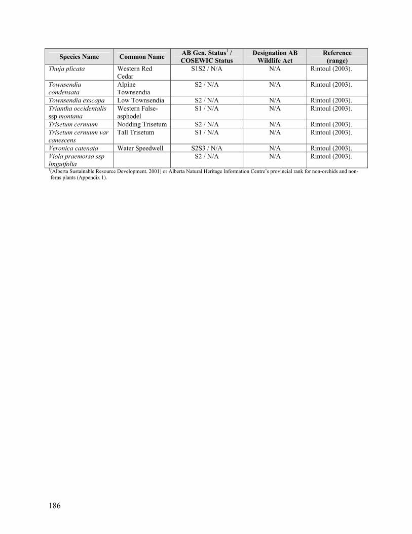
186
Species Name Common Name AB Gen. Status1 / COSEWIC Status
Designation AB Wildlife Act
Reference (range)
Thuja plicata Western Red Cedar
S1S2 / N/A N/A Rintoul (2003).
Townsendia condensata
Alpine Townsendia
S2 / N/A N/A Rintoul (2003).
Townsendia exscapa Low Townsendia S2 / N/A N/A Rintoul (2003). Triantha occidentalis ssp montana
Western False-asphodel
S1 / N/A N/A Rintoul (2003).
Trisetum cernuum Nodding Trisetum S2 / N/A N/A Rintoul (2003). Trisetum cernuum var canescens
Tall Trisetum S1 / N/A N/A Rintoul (2003).
Veronica catenata Water Speedwell S2S3 / N/A N/A Rintoul (2003). Viola praemorsa ssp linguifolia
S2 / N/A N/A Rintoul (2003).
1(Alberta Sustainable Resource Development. 2001) or Alberta Natural Heritage Information Centre�s provincial rank for non-orchids and non-ferns plants (Appendix 1).