sources of error in accuracy assessment of thematic land...

www.elsevier.com/locate/rse

Remote Sensing of Environment 90 (2004) 221–234

Sources of error in accuracy assessment of thematic land-cover maps

in the Brazilian Amazon

R.L. Powell a,*, N. Matzkea, C. de Souza Jr. a,b, M. Clarka, I. Numataa,L.L. Hessc, D.A. Robertsa

aDepartment of Geography, University of California, Santa Barbara, Ellison Hall 3611, Santa Barbara, CA 93106, USAb Instituto do Homem e Meio Ambiente da Amazonia Imazon, Caixa Postal 5101, Belem, PA 66613-397 Brazil

c Institute for Computational Earth System Science ICESS, University of California,Santa Barbara, CA 93106, USA

Received 29 August 2003; received in revised form 9 December 2003; accepted 13 December 2003

Abstract

Valid measures of map accuracy are critical, yet can be inaccurate even when following well-established procedures. Accuracy assessment is

particularly problematic when thematic classes lie along a land-cover continuum, and boundaries between classes are ambiguous. In this study,

we examined error sources introduced during accuracy assessment of a regional land-cover map generated fromLandsat ThematicMapper (TM)

data in Rondonia, southwestern Brazil. In this dynamic, highly fragmented landscape, the dominant land-cover classes represent a continuum

from pasture to second growth to primary forest. We used high spatial resolution, geocoded videography as a reference, and focused on second-

growth forest because of its potential contribution to the regional carbon balance. To quantify subjectivity in reference data labeling, we

compared reference data produced by five trained interpreters. We also quantified the impact of other error sources, including geolocation errors

between the map and reference data, land-cover changes between dates of data collection, heterogeneous reference samples, and edge pixels.

Interpreters disagreed on classification of almost 30% of the samples; mixed reference samples and samples located in transitional classes

accounted for a majority of disagreements. Agreement on second-growth forest labels between any two interpreters averaged below 50%, while

agreement on primary forest was over 90%. Greater than 30% of disagreement between map and reference data was attributed to geolocation

error, and 2.4% of disagreement was attributed to change in land cover between dates. After geocorrection, 24% of remaining disagreements

corresponded to reference samples with mixed land cover, and 47% corresponded to edge pixels on the classified map. These findings suggest

that: (1) labels of continuous land-cover types are more subjective and variable than commonly assumed, especially for transitional classes;

however, using multiple interpreters to produce the reference data classification increases reference data accuracy; and (2) validation data sets

that include only non-mixed, non-edge samples are likely to result in overly optimistic accuracy estimates, not representative of the map as a

whole. These results suggest that different regional estimates of second-growth extent may be inaccurate and difficult to compare.

D 2004 Elsevier Inc. All rights reserved.

Keywords: Error; Accuracy assessment; Brazilian Amazon; Second-growth forest

1. Introduction application. For example, in the tropics, an important

Thematic maps derived from remotely sensed data are

used in many applications, including as input parameters to

models, as source of regionally extensive environmental

data, or as basis of policy analysis. Meaningful and consis-

tent measures of thematic map reliability are necessary for

the map user to assess the appropriateness of the map data

for a particular application; additionally, the accuracy of the

thematic map may significantly affect the outcome of an

0034-4257/$ - see front matter D 2004 Elsevier Inc. All rights reserved.

doi:10.1016/j.rse.2003.12.007

* Corresponding author. Tel.: +1-805-893-4519; fax: +1-805-893-

3146.

E-mail address: [email protected] (R.L. Powell).

application of land-cover maps is assessing the rate and

extent of land-cover change to estimate the contribution of

tropical forest conversion to global and regional carbon

budgets. Accurate accounting of the carbon budget has

important implications for national policy aimed at comply-

ing with international treaties to reduce greenhouse gases

(Houghton, 2001). Currently, unquantified sources of un-

certainty in estimating the carbon flux of tropical forest

regions include the spatial extent of secondary forest (i.e.,

forest regrowth) and the associated rates of carbon seques-

tration (Houghton, 2003).

Measures of map accuracy are equally important for the

producer of a thematic map to analyze sources of error and

R.L. Powell et al. / Remote Sensing of Environment 90 (2004) 221–234222

weaknesses of a particular classification strategy. Yet, doc-

umenting map accuracy is not a straightforward task. While

individual measures of map accuracy are well established in

the literature (e.g., Congalton, 1991; Congalton & Green,

1999; Stehman, 1997a), considerable ambiguity remains

concerning the implementation and interpretation of themat-

ic map accuracy assessment. Uncertainties include the

selection of which accuracy measures to report, how to

interpret them, and the nature and quality of reference

samples. As a result, map quality remains ‘‘a difficult

variable to consider objectively’’ (Foody, 2002).

Fundamental to the challenge of accuracy assessment is

the problematic nature of thematic maps themselves, in that

thematic maps partition continuous landscapes into discrete,

mutually exclusive classes (Gopal & Woodcock, 1994).

While many distinct boundaries may exist on a landscape

(e.g., a forest at the bank of a river), virtually all environ-

ments include land-cover classes that represent segments of a

continuum (e.g., in the tropics, pasture to second-growth

forest to primary forest). The extremes of such classes may

be spectrally distinct and therefore easily separated; howev-

er, the boundaries between such classes can be arbitrary, and

distinguishing between the two classes becomes increasingly

difficult near the boundary (Gopal & Woodcock, 1994).

Even if classes are clearly defined and spectrally distinct,

a thematic map is based on the assumption that each region

represents a single land-cover class. However, all satellite

imagery used to derive thematic maps—regardless of the

spatial resolution of the sensor—will include mixed pixels

as a result of three situations. When classes are discrete or

easily separable, mixed pixels are located on the boarder

between them; when classes are portions of a continuous

landscape gradient, mixed pixels are located in the transition

zone between classes. Finally, mixed pixels can result when

subpixel objects—such as a road, building, or tree—are

present on the landscape (Cracknell, 1998; Fisher, 1997;

Foody, 1999). This may cause problems, not only in

interpreting the thematic map product, but also in collecting

reference data samples for accuracy assessment. Regardless

of the source of reference samples (e.g., ground surveys,

aerial photographs), human interpretation is almost always

required to assign a class label to the reference sample.

Consistent assignment of class labels may be confounded by

samples that occur on boundaries or in transition zones

between classes, or that include subpixel objects. The

frequency of mixed pixels is a function of both the spectral

complexity and the spatial fragmentation of the landscape,

and therefore the confidence level of an accuracy assess-

ment is compromised by an increasingly heterogeneous

landscape.

Estimation of the thematic accuracy of land-cover maps

by means of a set of labeled reference samples is based on

several assumptions: (1) that the reference data set is a

statistically valid sample of the mapped area; (2) that the

reference samples are accurately coregistered with the map;

(3) that the samples can be consistently and unambiguously

labeled as one of the map classes; (4) that each map pixel

corresponds to a single land-cover type; and (5) if time has

elapsed between acquisition of the map and reference data

sets, that land cover has not changed in the interim (Foody,

2002; Gopal & Woodcock, 1994; Lunetta et al., 2001). This

study examines the validity of these assumptions for the

accuracy assessment of a regional land-cover map derived

from Landsat Thematic Mapper (TM) imagery, using digital

aerial videography as the source of reference data. We select

as an example a land-cover map from a highly fragmented,

dynamic landscape in the southwest Brazilian Amazon. The

dominant classes represent a land-cover continuum, ranging

from pasture to second-growth forest to primary forest, and

the class of greatest interest is the transitional class, second-

growth forest, because of potential impact on the regional

carbon budget (Fearnside, 2000).

Our specific goals are twofold: First, we test the subjec-

tivity of assigning land-cover classes to samples of high

spatial resolution videography by comparing independent

interpretations of reference data and analyzing the sources

of disagreement between interpreters. Second, we assess the

disagreement between the thematic map and the highest

quality reference data set in light of the standard assump-

tions of accuracy assessment listed above. Many previous

studies have acknowledged that failing to meet any one of

these assumptions impacts accuracy assessment; we

strengthen these conclusions by quantifying the impact of

each assumption on the accuracy assessment measures

reported. Specifically, we quantify disagreements due to

the following factors: geolocation errors between the map

and the reference data, mixed reference samples, edge or

boundary pixels on the map, and change in land cover

between the collection of the reference data and the map

imagery.

2. Background

To evaluate the frequency and detail of accuracy assess-

ment reported in studies that map second-growth forest in

the Brazilian Amazon using remotely sensed data, we

reviewed 26 papers published in the refereed literature

between 1993 and 2003. The primary goal of secondary

forest mapping as presented in these papers could be divided

into three categories: (1) to map and assess the extent and

rates of forest clearing and regrowth; (2) to characterize the

spectral properties of second growth, especially to distin-

guish between age classes of second-growth forest; and (3)

to characterize field data to facilitate mapping second

growth with remotely sensed data (one paper). Study sites

ranged in scale from the entire Brazilian Amazon (approx-

imately 5 million km2) to less than 2500 km2, with almost

one-half of the studies in the latter category. While study

sites were distributed across the Brazilian Amazon, 12 of the

studies included sites in the state of Rondonia, in the

southwest Brazilian Amazon.

R.L. Powell et al. / Remote Sensing of Environment 90 (2004) 221–234 223

In our evaluation of accuracy reporting, we examined

whether and at what level of detail each study reports

accuracy and how clearly each study defines the thematic

classes mapped. Almost one-half of the papers (12) do not

include any discussion of the accuracy of the map products

that are developed or applied. Of the papers that do present

some discussion of accuracy assessment, eight include at

least one major methodological weakness. For example, six

papers select samples for the reference data set from within

homogeneous polygons defined in the field, and then treat

the samples as statistically independent. This results in

accuracy measures that are optimistically high (Foody,

2002). A second example of methodological weakness

occurs when class transition information from a time series

of classified imagery is used as reference data to validate the

age of mapped second growth. In all but one of these cases

(five of six papers), no discussion of the time series

accuracy is included. In other words, the reference data

are based on a second classified map (or series of classified

maps), which is taken as ‘‘truth’’ without any accuracy

assessment analysis.

Of our survey, only four papers clearly included randomly

selected reference samples collected from a combination of

high spatial resolution imagery and field data, rather than

from a second classified map (Ballester et al., 2003; Lu et al.,

2003a, 2003b; Roberts et al., 2002). However, three of these

studies report accuracy for classes using significantly fewer

than 50 reference sample points, a number recommended for

statistical robustness (Congalton, 1991), and the fourth does

not report an error matrix—only user’s, producer’s, and

overall accuracies. One other paper estimates the overall

accuracy of a time series by conducting accuracy assessment

for two different dates, using reference data collected during

two different field seasons, although the statistical indepen-

dence of the sample points is not discussed.

A second issue critical to the discussion of accuracy

assessment is the explicit definition of each thematic class.

In tropical forest environments, the main classes of inter-

est—pasture, second-growth forest, primary forest, and

most recently degraded forests—represent segments of a

continuum, and the boundaries between each class must be

prespecified. That is, pasture and cropland that are ‘‘aban-

doned’’ or not well maintained are rapidly invaded by

woody species, which develop into second-growth forest,

but the point at which land cover ceases to be ‘‘pasture’’ and

becomes ‘‘second growth’’ is essentially an arbitrary deci-

sion. On the other hand, while the distinction between

second growth and primary forest may be relatively clear

in ecological terms (Brown & Lugo, 1990), many research-

ers report that second growth becomes spectrally indistin-

guishable from primary forest on Landsat TM imagery after

approximately 15 years (Lucas et al., 2000; Mausel et al.,

1993; Nelson et al., 2000), although exceptions occur (e.g.,

Vieira et al., 2003).

Of the 26 papers surveyed, 14 included no specific

definition of second-growth vegetation, while eight included

a brief discussion of the dominant species present and/or

general structure of second-growth forest. Only three studies

(Lu et al., 2003a; Moran et al., 2000; Vieira et al., 2003)

included discussions of second-growth vegetation structure

that reported specific height measurements; another study

(Lu et al., 2003b) refers to the definitions presented by

Moran et al. (2000). Only one paper surveyed makes a clear

distinction between pasture and second-growth classes (Lu

et al., 2003a), although several discuss the relatively high

degree of confusion between the two classes (e.g., Ballester

et al., 2003; Roberts et al., 2002). Without clearly defined

classes, however, it is not possible to compare extents and

rates of land-cover change generated from different classi-

fication techniques or calculated for different regions be-

cause differences in such estimates may simply be a matter

of definition. In addition, clearly defined classes are needed

to extrapolate field measurements to larger regions using

maps derived from remotely sensed imagery, one of the

goals of the NASA-funded Large Scale Biosphere–Atmo-

sphere Experiment in Amazonia (LBA, 1997).

Similarly, without including a statistically rigorous ac-

curacy assessment with clearly detailed methods, confi-

dence in the thematic maps produced cannot be well

founded and comparison of classification techniques is

difficult. One of the limitations to conducting rigorous

accuracy assessment has been the collection of a sufficient

number of randomly selected samples for each map cate-

gory. This is especially an issue in tropical forests such as

the Brazilian Amazon, which contain vast tracts of land that

are virtually inaccessible from the ground. In such areas, it

is often simply not feasible to collect enough sample points

from ground-based surveys, and the only cost-effective and/

or feasible means of collecting enough independent samples

for regional-scale maps is to rely on high spatial resolution

remote sensing products, such as aerial photographs, aerial

videography, or satellite imagery (e.g., Ikonos or Quick-

Bird). In the past, such products have not been readily

available, and so accuracy assessment, when conducted,

could not necessarily meet the required number of indepen-

dent samples. Today, such data are available, and mapping

exercises can be expected to meet requirements for rigorous

accuracy assessment.

Measures of map accuracy are well established in the

literature (e.g., Congalton, 1991; Congalton & Green, 1999;

Stehman, 1997a; Story & Congalton, 1986). Most common-

ly, accuracy assessment involves the comparison of a

classified thematic map with the classification of randomly

selected samples of reference data (Stehman, 1997a). The

most widely used measures of accuracy are derived from an

error matrix (Congalton, 1991; Foody, 2002), which is a

table that compares counts of agreement between reference

and map data by class. The error matrix is used to generate

both descriptive and analytical statistical measures (Con-

galton, 1991). Descriptive measures of map accuracy pro-

vide the potential user of the final map product with a

measure of overall confidence in the map, as well as


measures of accuracy by class. Analytical statistical meas-

ures of map accuracy provide a means of comparing two

map products (Stehman, 1997a). Many researchers argue

that any thematic map product should report an error matrix

and include a thorough description of the reference collec-

tion process so that the user can analyze map accuracy in a

means appropriate to the intended application of the map

product (Foody, 2002; Stehman, 1997a; Story & Congalton,

1986). However, the results reported in an error matrix

should be interpreted with caution, as the error matrix

measures the degree of agreement between the reference

data and the map data, which is not necessarily equivalent to

the degree of agreement between the map product and

reality (Foody, 2002). If the error matrix is incorrect because

the reference data are less than perfect, all accuracy meas-

ures derived from it are suspect (Congalton, 1991). As a

result, any accuracy assessment should involve close scru-

tiny of the reference data.

3. Methods

3.1. Study site

The study area includes two Landsat TM scenes (ap-

proximately 54,000 km2) over the central portion of the state

Fig. 1. Map showing study site and the location of the Landsat TM scenes. Vid

superimposed on the classified map used for accuracy assessment analysis. Schema

flight line. Shaded pixels were evaluated as reference samples.

of Rondonia in the southwest Brazilian Amazon (Fig. 1),

where deforestation rates have been among the highest in

Brazil throughout the decades of the 1980s and 1990s

(Alves, 2002). Elevation in the region varies between 100

and 1000 m, including some areas with steep terrain. Annual

rainfall ranges between 1930 and 2690 mm/year, and there

is a pronounced dry season from approximately June

through October (Gash et al., 1996). Natural land cover is

predominantly tropical moist forest, which covered approx-

imately 89% of the state area prior to deforestation, and

there are also significant areas of natural savanna shrublands

(Skole & Tucker, 1993).

Modern Brazilian exploration and settlement in the

region increased exponentially after the 1968 opening of

the Cuiaba-Porto Velho (BR-364) highway (Moran, 1993),

which bisects the study area, and large tracts of land on

either side of the highway were included in government-

sponsored colonization projects, first initiated in 1971

(Pedlowski et al., 1997). The majority of properties are

relatively small ( < 100 ha) and are located in close prox-

imity to the major highway and secondary roads (Alves et

al., 1999; Alves & Skole, 1996), resulting in a ‘‘fish-bone’’

pattern of deforestation that is commonly associated with

frontier colonization projects (Geist & Lambin, 2001).

Deforestation in Rondonia has largely been driven by the

conversion of land for agriculture, especially pasture, with

eography flight lines from which reference data samples were derived are

tic in lower right shows the placement of cluster samples on the videography


some logging and mining activities (Moran, 1993; Pedlow-

ski et al., 1997). The region covered in this study includes a

range of pasture and second-growth ages, as well as a

gradient in the degree of pasture maintenance.

Data for the Ji-Parana Landsat TM scene (P231, R67)

were acquired in August 1999, while for the Ariquemes

scene (P232, R67), data from July 1998 and October 1999

were combined due to cloud contamination. The Landsat

scenes were coregistered to digital base maps supplied by

Brazil’s Instituto Nacional de Pesquisas Espaciais (INPE,

2003). The scenes were intercalibrated using relative radio-

metric calibration techniques to account for differences in

atmospheric conditions between scenes and between dates

(Furby & Campbell, 2001). As described by Roberts et al.

(1998, 2002), land cover was mapped using a multistage

process based on spectral mixture analysis. Endmember

fractions and root mean square error values were used to

train a binary decision tree classifier. The rules generated by

the decision tree were used to classify both images into

seven classes: primary forest, pasture, green pasture, sec-

ond-growth forest, water, urban/bare soil, and rock/savanna.

For the purpose of accuracy assessment, we combined the

pasture and green pasture classes, and did not include the

rock/savanna class because of its scarcity on the landscape.

Reference data were visually interpreted from digital

aerial videography collected over Rondonia in June 1999,

as part of the Validation Overflights for Amazon Mosaics

(Hess et al., 2002). Wide-angle and zoom videography were

collected simultaneously, with average swath widths of 550

and 55 m, and average pixel dimensions of 0.75 m and 7.5

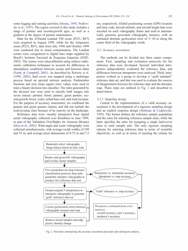
Fig. 2. Flowchart summarizing the accuracy asse

cm, respectively. Global positioning system (GPS) location

and time code, aircraft attitude, and aircraft height data were

encoded on each videography frame and used to automat-

ically generate geocoded videography mosaics, with an

estimated absolute geolocation error of 5–10 m along the

center third of the videography swath.

3.2. Accuracy assessment

The methods can be divided into three major compo-

nents. First, sampling and evaluation protocols for the

reference data were developed. Second, individual inter-

preters independently evaluated the reference data, and

differences between interpreters were analyzed. Third, inter-

preters worked as a group to develop a ‘‘gold standard’’

reference data set, and this was used to evaluate the sources

of disagreement between the reference data and the thematic

map. These steps are outlined in Fig. 2 and described in

detail below.

3.2.1. Sampling design

Central to the implementation of a valid accuracy as-

sessment is the development of a rigorous sampling design

and an explicit response design (Stehman & Czaplewski,

1998). The former defines the reference sample population

and the rules for selecting reference sample units, while the

latter specifies the rules for assigning a single land-cover

class to each sample unit. The only rigorous sampling

scheme for selecting reference data in terms of scientific

objectivity, as well as in terms of meeting the criteria for

ssment procedure and subsequent analysis.

Table 1

Proportion of reference samples by class compared to proportion of total

classified map pixels by class

Pfor (%) Sfor (%) Past (%) Other (%)

Reference samples 54 14 30 2

Classified map 66 7 25 2

Pfor = primary forest; Sfor = second-growth forest; Past = pasture.


accuracy assessment measures such as the kappa statistic, is

that based on random sampling (Congalton, 1991; Stehman

& Czaplewski, 1998). However, as is commonly the case in

the collection of reference data, two factors confound our

ability to implement a true simple random sampling design.

First, the population of reference sample units was limited

to points along the videography flight lines, and the flight

lines were not planned according to a random sampling

strategy. Second, some classes are much more abundant

than others on the landscape (e.g., primary forest is the

dominant class in the study area, followed by pasture, with

significantly smaller areas covered by second-growth for-

est). Therefore, a simple random sampling design could

result in very small numbers of samples for the secondary

forest class.

We addressed the first issue with the following observa-

tions: The flight lines crossed both scenes several times and

were designed to cover a diversity of land-cover types. As

can be seen in Fig. 1, the flight lines cross areas of high

heterogeneity and avoid large areas of primary forest in the

eastern and western portions of the study area. We therefore

assumed that the videography data were representative of

the target classes in the study area, and that our findings of

class accuracy within the videography subregion could be

generalized to the entire map extent. This assumption was

also supported by the authors’ combined general knowledge

of the area based on prior field work. In addition, the

population of potential samples represented by the videog-

raphy coverage was quite large, as the flight lines covered a

distance of approximately 800 km over the study area and

included a total of approximately 3 h of flying time,

resulting in a sample population of 10,800 one-second

mosaics. Given an average swath width of 0.55 km, this

represents an area of 440 km2, equivalent to almost 1% of

the entire study area.

We addressed the second issue by implementing a

modified version of stratified random sampling. The flight

lines that cross the two scenes were segmented according to

dominant land-cover class present, and image frames were

extracted from each segment based on their randomly

selected recorded time codes. Image frames were sampled

more intensively from segments with more heterogeneous

land cover. While we did not achieve an equal distribution

of sample points by class (see Table 4 for a distribution of

samples by count), we were able to capture sufficient

numbers of samples (i.e., >50 as recommended by Con-

galton, 1991) for the three classes of greatest interest:

primary forest, pasture, and second-growth forest. Finally,

despite the limitations imposed on our sampling design, the

distribution by class of sample points included in the

reference data set closely reflects the proportion of classified

map pixels in the study area (Table 1), a condition for

establishing reliable estimates of individual class accuracy

and overall map accuracy (Richards, 1996). This strength-

ens the claim that the reference data set is representative of

the map as a whole.

The next step in designing a sampling protocol is to

define the sampling unit (i.e., the unit that links the

reference data to the classified map) (Stehman & Czaplew-

ski, 1998). Currently, there is no consensus in the literature

concerning the selection of the sampling unit size; however,

there is some agreement that the sample unit selected should

correspond to the mapping objective (Congalton & Green,

1999; Plourde & Congalton, 2003). In our case study, the

mapping objective was per-pixel characterization of land-

cover type. We therefore chose to use a 30-m pixel centered

on the videography mosaic as the sample unit, and note the

following advantages: (a) the pixel sample is physically

correlated with the minimum mapping unit of the Landsat

TM imagery, and therefore that of the classified map; (b)

using a pixel sample unit allowed us to assess the number of

mixed reference pixels and the number of edge sample

pixels on the map; and (c) as the videography mosaics

generated for analysis are quite large relative to the size of a

Landsat pixel, using a pixel sample unit allowed us to

collect more than one sample per mosaic (discussed in

detail below). Some researchers have argued that the geo-

location errors between the reference and map data com-

pound error in accuracy assessment when a sample unit on

the order of the minimum mapping unit is used (e.g.,

Plourde & Congalton, 2003). However, Stehman and Cza-

plewski (1998) argue that as long as boundary and edge

pixels are included in the accuracy assessment analysis,

geolocation error can be ‘‘equally problematic whether the

sampling unit is a pixel, polygon, or larger area.’’ In

addition, using sample units larger than the minimum

mapping unit in a heterogeneous landscape increases the

probability that the sampling unit includes more than one

land-cover type, and therefore complicates the response

design (i.e., how a land-cover class is assigned to the

sampling unit).

Mosaic construction is quite time-consuming, and each

mosaic is large relative to the size of the sampling unit.

Mosaics were approximately 300–900 m in each dimension

(equivalent to 10–30 Landsat pixels), depending on the

altitude of the aircraft. In an attempt to utilize more of the

information available on each mosaic, we employed a one-

stage cluster sampling method (Stehman, 1997b). Cluster

sampling involves two levels of sampling units: first, the

cluster itself (i.e., the primary sample unit), which is

centered on a randomly selected location; and second, the

fixed arrangement of secondary sample units, which make

up the cluster. Each sample unit within the cluster is treated

as an independent sample (Stehman & Czaplewski, 1998).


For this study, videography flight lines were randomly

sampled by flight timecode, and georectified mosaics were

constructed from wide-angle videography frames covering 1

s (30 frames) of aircraft flying time. Mosaics were printed at

a map scale of 1:2000 using a fine-resolution laser color

printer. A 5� 5 grid of 30-m pixels printed on a transpar-

ency was superimposed and centered on each mosaic. The

center and four corner pixels were collected as reference

samples, for a total of five samples per mosaic (Fig. 1). Non-

adjacent sample units were selected for analysis in order to

reduce autocorrelation between samples of the same cluster.

A total of 158 mosaics, generating 790 sample points, were

included.

3.2.2. Response design

The response design consists of two components: the

evaluation protocol, which details the criteria and procedure

to determine the land-cover type(s) within each sampling

unit; and the labeling protocol, which specifies how a single

class is assigned to the sampling unit (Stehman & Czaplew-

ski, 1998). Our goal in designing an evaluation protocol was

to develop explicit definitions of each land-cover class

based on physical characteristics. Clearly demarcating class

boundaries was a deliberate effort to increase consistency

between interpreters, as well as to provide a basis for

comparing our map product with other thematic maps.

Because pasture, second-growth forest, and primary forest

represent a continuum of vegetation cover, boundaries

between each class were delimited based on prespecified

physical criteria instead of current land use or age since cut.

Interpretation of land cover based on current or past land use

was avoided because such interpretations are subjective and

have no direct correlation to a specific spectral signature.

The class descriptions developed for the reference data

evaluation protocol, presented in Table 2, are based on

height, vegetation structure (woody vs. herbaceous), and

canopy cover (continuous vs. sparse). While height is not

directly measurable from the videography mosaics, other

characteristics that are correlated with vegetation height are

detectable. In particular, crown diameter and shadows were

used to infer vegetation height.

Table 2

Class definitions for evaluation protocol

Class Criteria

Primary forest Trees >20 m in height,

continuous canopy

Second-growth forest Shrubs >2 m in height,

trees < 20 m in height,

perennial crops

Pasture Shrubs < 2 m in height,

herbaceous vegetation,

sparse canopy, annual

crops

Urban/bare soil Human-built structures,

roads, bare soil

Water Open water surfaces

Interpreters viewed each sample in the context of the

entire 1-s mosaic and recorded the percentage of all land-

cover classes present in each sample unit. The labeling

protocol was simple: Each sample unit was assigned the

class of majority cover, based strictly on the land cover

located directly within the boundaries of the sample unit.

For example, if the sample unit landed on an isolated tree

surrounded by pasture, the sample would be assigned the

class of either primary forest or second-growth forest,

depending on the tree height, as inferred by crown size.

As each sample had to be assigned to one—and only—

class, interpreters had to make judgment calls when

sample units had near 50–50% splits between two clas-

ses. An application of the response design is presented in

Fig. 3.

3.2.3. Videography interpretation

Five researchers were trained in photointerpretation of

this region. Three of the researchers had prior experience

working in the Amazon region of Brazil; the other two had

extensive experience working in tropical forests in other

regions of the world. An effort was made to increase

consistency between interpreters. After all interpreters

agreed on the criteria for each class based on the simple

biophysical descriptions presented in Table 2, they practiced

classifying the videography as a group on mosaics not

included in the accuracy assessment. After the training

period, each interpreter independently analyzed the same

samples on all mosaics included in the analysis. Each set of

reference data (one per interpreter) was compared to the

classified map, as well as to each other. This resulted in 10

pairwise comparisons between interpreters, and five pair-

wise comparisons between interpreters and the map.

Error matrices were central to all comparisons and used

to derive the following descriptive and statistical accuracy

measures: overall agreement, user’s accuracy, producer’s

accuracy, the kappa coefficient of agreement, and kappa

variance (Congalton, 1991; Congalton & Mead, 1983;

Hudson & Ramm, 1987). All of the accuracy measures

except kappa variance are identical for simple random

sampling and cluster sampling. However, the kappa vari-

ance formula for cluster sampling must incorporate auto-

correlation between samples within the same cluster; thus,

kappa variance is expected be higher for cluster sampling

than for simple random sampling (Stehman, 1997b). Kappa

and kappa variance were used to test whether error matrices

from each interpreter–map comparison were statistically

different (Congalton & Mead, 1983; Hudson & Ramm,

1987).

As a final step, the interpreters reassembled as a group

and produced the reference data set used for the final

accuracy assessment analysis of the classified map, hereafter

referred to as the ‘‘gold’’ reference set. Reasons for dis-

agreement between the independent videography interpre-

tations were recorded and analyzed. In cases where the

group continued to disagree or remained uncertain, the

Fig. 3. An illustrated application of the response design.


zoom videography was accessed to clarify the vegetation

structure on the ground.

3.2.4. Evaluation of reference data map disagreement

The gold reference set was compared to the map data by

generating an error matrix and associated accuracy meas-

ures. The error matrix represents the degree of agreement/

disagreement between the highest quality reference data set

and the map data; however, the error matrix also incorpo-

rates sources of disagreement between the two data sets,

which may not reflect map accuracy, namely georegistration

errors and change in land cover between collection of the

videography and collection of the Landsat imagery. To

quantify the degree to which each of these errors affected

the accuracy assessment, we visually compared each 1-s

mosaic to the classified map overlaid with the coordinates of

the mosaic centers and manually adjusted clear errors of

georegistration. Where additional context was needed, we

observed longer portions of the wide-angle videography.

Similarly, we visually inspected areas of potential change

(based on reference and map classifications) by comparing

such locations to classified maps from the previous year,

which had been generated following identical classification

procedures (Roberts et al., 2002).

Finally, we assessed the impact of including mixed

reference pixels and map edge pixels in the accuracy

assessment. Mixed reference pixels were identified by the

interpreters as a group and consisted of any sample unit that

contained more than one land-cover type based on videog-

raphy interpretation; samples that fell in transitional zones

were not included in this count. Edge pixels were identified

as any map pixel corresponding to a sample unit that

bordered a map pixel of a different class along one of its

cardinal directions. Mixed reference samples, map edge

pixels, and change pixels were determined independently

from each other, and, in some cases, a sample fell into more

than one group. For each category of ‘‘corrections’’ to the

reference data, an error matrix and associated accuracy

parameters were generated. Once we accounted for dis-

agreements due to geolocation errors, change between dates,

mixed reference samples, and edge pixels on the map, we

assumed the remaining disagreement between the reference

data and the map was due to classification error. We

analyzed the remaining error for systematic trends, as well

as to identify weaknesses in the current classification

scheme.

4. Results and discussion

4.1. Interpreter disagreement

At least one interpreter disagreed with the others on the

assignment of class labels for almost 30% of all samples.

The range of overall agreement between any two inter-

preters spanned almost 10% (Table 3), with the highest

agreement just under 90%. Because there is no reference

standard when comparing two interpreters, agreement be-

tween each class was determined by selecting the lower

producer’s or user’s accuracy for that class. Agreement

varied substantially by class: Average agreement between

two interpreters for the second-growth class was less than

50%, while average agreement for the primary forest class

was 92%, and for pasture was 81%.

Upon group review, many sources of interpreter dis-

agreement could clearly be traced to human error. In some

cases, an interpreter misinterpreted the printout image

because the quality of the printout had been compromised

Table 3

Summary of interpreter agreement (total agreement and agreement by class)

N= 790 samples Min Max Average

Interpreter vs. interpreter (%) 81.4 89.6 86.0

Second-growth forest (%) 32.0 69.7 48.8

Pasture (%) 72.4 88.0 80.6

Primary forest (%) 86.4 95.5 92.1

Interpreter vs. map (%) 71.3 74.6 72.4

Interpreter vs. map (j) 0.551 0.574 0.549

Minimum, maximum, and average agreements for pairwise comparisons are

reported.


in some way, such as differences between the color printouts

and the true color of the image, blurring due to badly

warped mosaics, or shadows due to cloud cover. Another

source of human error was recording mistakes, including

recording the wrong class label code, reversing the order of

the samples within a cluster, or misorienting the overlay on

the videography printout. However, many disagreements

were ‘‘unavoidable’’ in the sense that they resulted from

differences of opinion among interpreters. These differences

of opinion can be subdivided into two categories: disagree-

ments about land-cover types and disagreements about land-

cover percentages.

Despite explicit criteria for the identification of land-

cover type, interpreters did not always label the same

sample as the same land-cover class. The real world presents

ambiguous and intermediate cases, and when the land-cover

classes being identified are continuous (e.g., pasture, sec-

ond-growth forest, and primary forest), visually drawing a

precise line between classes can be difficult, even given

Fig. 4. Examples of clear and ambiguous land-cover classes from aerial videogra

classes: A= primary forest; B = second-growth forest; C = perennial crops (i.e., sec

not so clearly distinguished: X= second-growth forest; Y= ambiguous class (i.e.,

specific criteria. Over 50% of interpreter disagreement was

between pasture and second-growth classes, and almost

30% of interpreter disagreement was between second-

growth and primary forest classes. Quite often, these dis-

agreements would occur when sample boxes fell on edges

between two classes or along transition zones. Videography

samples of clearly labeled and ambiguous land cover are

presented in Fig. 4.

Even if interpreters agreed on the land-cover classes

found in a sample unit, the assignment of percentages was

a somewhat subjective decision. Almost 50% of the total

disagreement between interpreters occurred when there was

mixed land cover in a sample unit, and over 70% of those

samples identified by at least one interpreter as having more

than one land-cover type resulted in interpreter disagree-

ment. This was particularly an issue when the sample unit

was nearly evenly divided between two land-cover classes,

or contained more than two land-cover classes. In these

situations, small differences in the interpretation of percent

cover could result in differences in the majority land-cover

class, and the class labels assigned to the sample unit would

differ.

Despite the wide range of disagreements between inter-

preters, the range of overall percent accuracy for each

interpreter compared to the map is relatively small (Table

3). The difference between the overall accuracy for each

interpreter was statistically tested using kappa and kappa

variance and, in all cases, pairwise differences were not

significant ( p < 0.05), implying that using the reference data

of any individual interpreter would produce accuracy

parameters that were equally valid. This result supports

phy mosaics. On the mosaic at left, land cover can be clearly assigned to

ond-growth forest); D = pasture. On mosaic at right, land-cover classes are

transitional zone between pasture and second-growth forest).

Table 4

Error matrices

Classification Reference data

dataPfor Past Sfor Watr Urbn Row

total

User’s

Version 1: overall accuracy—75.4%

Map Pfor 351 3 19 3 0 376 93.4

data Past 18 205 61 0 1 285 71.9

Sfor 51 23 29 0 0 103 28.2

Watr 3 0 0 9 0 12 75.0

Urbn 0 7 5 0 2 14 14.3

Column

total

423 238 114 12 3 790 –

Producer’s 83.0 86.1 25.4 75.0 66.7 – –


Map Pfor 374 0 10 0 0 384 97.4

data Past 5 214 46 0 0 265 80.8

Sfor 45 18 54 0 0 117 46.2

Watr 0 0 0 12 0 12 100.0

Urbn 0 7 2 0 3 12 25.0

Column

total

424 239 112 12 3 790 –

Producer’s 88.2 89.5 48.2 100.0 100.0 – –


Map Pfor 374 0 10 0 0 384 97.4

data Past 0 215 36 0 0 251 85.7

Sfor 45 18 54 0 0 117 46.2

Watr 0 0 0 12 0 12 100.0

Urbn 0 4 0 0 3 7 42.9

Column

total

419 237 100 12 3 771 –

Producer’s 89.3 90.7 54.0 100.0 100.0 – –


Map Pfor 369 0 10 0 0 379 97.4

data Past 5 166 23 0 0 194 85.6

Sfor 45 10 39 0 0 94 41.5

Watr 0 0 0 9 0 9 100.0

Urbn 0 5 2 0 1 8 12.5

Column

total

419 181 74 9 1 684 –

Producer’s 88.1 91.7 52.7 100.0 100.0 – –


Map Pfor 320 0 4 0 0 324 98.8

data Past 2 186 35 0 0 223 83.4

Sfor 20 8 17 0 0 45 37.8

Watr 0 0 0 9 0 9 100.0

Urbn 0 2 1 0 1 4 25.0

Column

total

342 196 57 9 1 605 –

Producer’s 93.6 94.9 29.8 100.0 100.0 – –


Map Pfor 316 0 3 0 0 319 99.1

data Past 2 147 17 0 0 166 88.6

Sfor 20 4 12 0 0 36 33.3

Watr 0 0 0 9 0 9 100.0

Urbn 0 1 1 0 0 2 0.0

Column

total

338 152 33 9 0 532 –

Producer’s 93.5 96.7 36.4 100.0 n/a – –

Table 4 (continued)

Classification Reference data

dataPfor Past Sfor Watr Urbn Row

total

User’s


Map Pfor 316 0 3 0 0 319 99.1

data Past 0 147 11 0 0 158 93.0

Sfor 20 4 12 0 0 36 33.3

Watr 0 0 0 9 0 9 100.0

Urbn 0 1 0 0 0 1 0.0

Column

total

336 152 26 9 0 523 –

Producer’s 94.1 96.7 46.2 100.0 n/a – –

For version 1, the reference samples and map data were compared with no

corrections. For version 2, the reference data set was geocorrected relative

to the classified map. For each subsequent version, an additional

‘‘correction’’ was applied to the reference data set, as summarized in

Table 5.

Class labels are as follows: Pfor = primary forest; Past = pasture; Sfor =

second-growth forest; Watr =water; Urbn = urban/construction/bare soil.


the assertion that there were no systematic biases between

interpreters, and that, most likely, disagreements were

related to the difficulty of evaluating and labeling samples,

not to fundamental differences in implementation of the

evaluation and labeling protocols. However, the disagree-

ment between interpreters has significant implications for

the assessment of map accuracy. In particular, the class of

greatest interest, second-growth forest, had less than 50%

average agreement between all interpreters. As confidence

in the reference data set for that class remains quite low, we

can have only limited confidence in the map accuracy

measures reported for that class. Even after group reevalu-

ation of the reference data set to create the gold standard

reference, disagreement on class assignments remained,

particularly for second-growth forest.

4.2. Reference sample accuracy

Comparing the gold reference set with the map (version 1)

produced higher overall percent accuracy than any reference

data set generated by an individual interpreter. In addition,

the user’s and producer’s accuracies were as high or higher

than any individual reference set for all classes. Yet, the

overall percent accuracy remained relatively low at 75.4%,

and the accuracy of the second-growth class remained less

than 30% for both user’s and producer’s accuracies. The

resulting error matrix is reported in Table 4, and evaluation

of the types of confusion recorded indicated a source of

disagreement other than misclassification. For example,

several reference pixels in the water class were classified

on the map as primary forest—an error we were confident

was not due to misclassification because the two classes are

spectrally quite distinct. Similarly, pasture reference pixels

classified as primary forest and urban/soil classified as

second-growth forest represent errors that are unlikely to

be due to misclassification, as the paired classes are also

spectrally distinct from each other. Therefore, the error

Table 5

Influence of reference data ‘‘corrections’’ on map accuracy

Version Corrections to reference

data set

Number of

samples

% Overall

agreement

1 None 790 75.4

2 Geocorrection 790 83.2

3 Geocorrection; remove

change pixels

771 85.3


mixed reference samples

684 85.4


map edge pixels

605 88.1


mixed reference and map

edge pixels

532 91.0


mixed, edge, and change

pixels

523 92.5


reported in these three cases was hypothesized to be due to

geolocation errors between the reference data and the map.

The next version of the accuracy assessment involved the

geocorrection of the reference data relative to the map

(version 2) by manually adjusting all clear georegistration

errors between the reference data and the map. The result

was a substantial increase in overall percent accuracy, to

83.2%, as well as a notable increase in user’s and producer’s

accuracies for all classes (Table 4). In addition, almost no

confusion between the three pairs of spectrally distinct

classes mentioned above was recorded, and the results of

version 3 (below) indicated that the remaining confusion

between second growth and the urban/soil class was due to

change between the two dates. Of the original total dis-

agreement between the gold reference set and the map, 32%

could be attributed to geolocation error, and the total

number of disagreements between the map and reference

data decreased from 195 to 132. Geolocation error between

the map product and reference data had such a large impact

on the total error because of the high degree of heteroge-

neity and fragmentation in portions of the landscape repre-

sented in the map. Especially in regions impacted by human

activity, no single class dominates, and in these areas, the

chances of a reference sample landing on a boundary

between classes are relatively high. As a result, a slight

shift in geolocation relative to the map may result in quite

different map classes.

All subsequent versions of the accuracy assessment

applied ‘‘corrections’’ to the geocorrected reference sam-

ples. Version 3 of the accuracy assessment involved remov-

ing all pixels that changed land-cover class between the date

of videography acquisition and the date of image acquisi-

tion. The 19 pixels removed from the sample by this

criterion represented 2.4% of the total reference samples,

but accounted for 14% of the error remaining after geo-

correction, implying that change pixels are a potentially

important source of error in a dynamically changing land-

scape. Although the removal of change pixels resulted in

only a slight increase in overall percent accuracy, to 85.3%,

user’s and producer’s accuracies increased for most classes

(Table 4).

After geocorrection, 24% of the remaining disagreements

between the gold reference set and the map corresponded to

reference samples with mixed land cover, and 47% corre-

sponded to edge pixels on the classified map. We assumed

that edge pixels on the map have a high probability of either

being mixed pixels located on boundaries or being located

in a transitional zone between classes. The error associated

with mixed sample pixels and map edge pixels is potentially

more an artifact of partitioning continuous land-cover types

into discrete classes than a result of ‘‘misclassification’’ per

se. Confidently assigning the source of such error as

misclassification of the map or as misinterpretation of the

reference data may not be possible.

Next, we sequentially excluded these categories of

problematic samples from the reference data set to assess

the impact of each on the accuracy assessment of the map.

Version 4 removed reference samples with mixed land

cover from the reference data set (i.e., samples with more

than one land-cover class on the videography). Version 5

removed reference samples that corresponded to edge

pixels on the map (i.e., pixels on the border between

two classes on the map). Version 6 excluded both mixed

reference samples and edge pixels on the map. Version 7

excluded all three categories of problematic samples:

mixed samples, edge map pixels, and pixels that had

changed between dates. Error matrices for all versions

are presented in Table 4, and a summary of the ‘‘correc-

tions’’ applied to the reference data and the resulting

overall agreements is presented in Table 5. Geocorrection

and removing change pixels led to a substantial increase in

overall percent accuracy (from 75% to 85%), as well as

notable increases in the producer’s and user’s accuracies

for all classes (Table 4). Removing mixed reference

samples and map edge pixels from the accuracy assess-

ment analysis resulted in a similar jump of overall percent

accuracy (from 85% to 93%). However, this increase in

percent accuracy leads to both practical problems and

theoretical shortcomings. Excluding edge pixels and mixed

reference samples significantly reduces the number of

samples in several classes, and eliminates all samples from

the urban/soil class. A significant portion of second-growth

samples is also eliminated, resulting in a decrease in user’s

and producer’s accuracies for that class.

The theoretical problem presented by excluding edge

and mixed pixels from analysis is related to the fact that

the landscape we have mapped is quite heterogeneous in

areas dominated by human activity. Such areas account for

three of the five classes included in the accuracy assess-

ment, and we assume that a large portion of pixels in such

areas will be mixed pixels located on class boundaries or

in transitional zones. Smith et al. (2002) have noted that

as landscape heterogeneity (i.e., the number of classes within

a defined area) increases, thematic map accuracy decreases;

Table 6

Summary of disagreement after geocorrection and removal of change pixels

Total disagreements = 115 Number of

samples

Total

disagreement (%)

Between primary and second growth 55 47.8

Reference = Pfor, map = Sfor 45 39.1

Reference = Sfor, map = Pfor 10 8.7

Between pasture and second growth 54 47.0

Reference = Past, map = Sfor 18 15.7

Reference = Sfor, map = Past 36 31.3

Pfor = primary forest; Sfor = second-growth forest; Past = pasture.


similarly, as average patch size (i.e., the number of contig-

uous pixels belonging to the same class) decreases, accuracy

also decreases. Although we have not directly measured

landscape heterogeneity or fragmentation, it is clear that there

is a negative relationship between these variables and map

accuracy. However, any fair representation of map accuracy

must include all pixels in the sample population for accuracy

assessment, and failure to do so will result in accuracy

measures that can only be applied to larger regions of

homogeneous land cover within the scene (Foody, 2002;

Stehman & Czaplewski, 1998). We therefore purport that

version 3 of our accuracy assessment, which includes geo-

correction of the two data sets and removal of pixels that have

changed between the two collection dates, is the most

representative estimate of map accuracy.

Error matrices for each version of the accuracy assess-

ment are presented in Table 4 to highlight the importance

of reporting pixel counts rather than a normalized matrix

(Foody, 2002; Stehman, 1997a). Pixels counts can provide

the map user with additional information about the degree

of confidence and robustness of accuracy measures by

class—information that is not sufficiently captured in

percentages. Such information allows the map user to

evaluate the accuracy of the map product with a specific

application in mind (Stehman, 1997a). In particular, the

map user would be aware of classes that are underrepre-

sented in the sampling scheme and, in turn, which accuracy

measures may be less certain. In this example, the water

and urban/soil classes (and in version 7, second-growth

forest) are underrepresented, and their accuracy cannot be

stated with the same degree of confidence as that of other

classes. In addition, including pixel counts can make it

easier to identify nonsensical errors that may reflect the

quality of the reference data, rather than misclassification

error of the map.

Investigating the sources of error in our most represen-

tative assessment of accuracy (version 3) can inform further

refinement of the classification process, as the majority of

classification errors do not appear random. Approximately

95% of the total error involves disagreement between

second-growth forest and other classes; 48% of the total

error is disagreement between primary forest and second-

growth forest, and 47% is disagreement between second-

growth forest and pasture (Table 6). The former represents a

systematic error; sunlit slopes of primary forest were con-

sistently classified as second-growth forest. The brightness

of the vegetation due to illumination effects causes those

pixels to have spectral properties similar to second growth

(Roberts et al., 2002; also note this error). Such an error

could be easily corrected with a digital elevation model

(DEM) of sufficient spatial resolution. We are currently in

the process of correcting the error using recently released

Shuttle Radar Topography Mission (SRTM) data (Rabus et

al., 2003).

The disagreement between pasture and second growth

is not so straightforward and could have several explan-

ations. First, the classifier was designed based on spectral

properties of known land-cover patches, not on the phys-

ical structural criteria presented in Table 2. It is possible

that the classifier is consistent throughout the scene, but

responds to different criteria than those used by the

videography interpreters. A second possibility is that the

reference data are consistently wrong (i.e., that it was not

possible to visually distinguish between degraded pasture

and young second growth on the videography based on the

arbitrary structural division between the two classes for-

mulated in the response design). A third possibility is that

geolocation remains a major issue. The geospatial accuracy

of the Landsat TM scenes was untested and the videog-

raphy was roughly accurate to 5–10 m in the center pixel

of our sampling clusters. The spatial mismatch between

these data sources translates into classification error, par-

ticularly in transition zones, because class assignment (for

the videography interpretation and/or for the image clas-

sification) is heavily dependent on the percent cover

within a given sample unit. A final possibility is that, in

some cases, the two classes are spectrally indistinguish-

able, an artifact of using arbitrary boundaries to partition

continuous land cover (pasture to second growth). In any

case, without extensive collection of precisely defined

training sites to refine the rules of the decision tree

classifier, the confusion between pasture and second

growth seems to mark the limits of our classification

scheme.

5. Conclusion

Throughout this project, we have built a case that it is

essential to explicitly define thematic map classes in terms

of biophysical parameters, both to promote consistency

within a single reference data set and to provide a basis

for comparing classification techniques or maps from dif-

ferent regions. However, explicit definitions of thematic

classes are necessary, but not sufficient, criteria to insure

objective interpretation of land-cover types. Labels of land-

cover types along a continuum are more subjective and

variable than commonly assumed, especially for transitional

classes. In the case presented, five independent interpreters

agreed less than 50% of the time in assigning second-growth


forest labels to reference samples. Disagreement of this

magnitude has serious implications for the scientific appli-

cation of a thematic map that includes such a transitional

class. In the case of the Amazon Basin, maps of second-

growth vegetation are important for assessing the contribu-

tion of regrowth to the regional carbon budget (Fearnside,

2000), but the apparent subjectivity in labeling reference

data as second-growth forest lowers confidence in the

overall estimate of carbon flux. Additionally, disagreement

between interpreters for classes along a landscape gradient

suggests the importance of employing multiple interpreters

to produce the reference data used for accuracy assessment.

We have demonstrated that reference data produced by a

group of interpreters boost reference accuracy over a data

set produced by a single interpreter.

Our analysis demonstrates that validation data sets that

include only nonmixed, nonedge samples are likely to

result in overly optimistic accuracy estimates that are not

representative of the map as a whole. Although we did not

directly quantify landscape heterogeneity or fragmentation,

it is clear that accuracy decreases with increasing hetero-

geneity and/or with increasing fragmentation, following the

conclusions of Smith et al. (2002). Extensive portions of

the thematic map in our case study include a heteroge-

neous and fragmented landscape, and therefore the exclu-

sion of such pixels from the accuracy assessment analysis

cannot be justified. On the other hand, error that results

from including mixed reference samples and map edge

pixels cannot easily be assigned to either incorrect inter-

pretation of reference samples or incorrect classification of

image data, and such error may well be an intrinsic

problem of dividing a continuous landscape into discrete

classes. How to effectively account for such pixels in

accuracy assessment is an important direction of future

research (Foody, 2002).

Finally, the analysis of accuracy assessment in this case

study demonstrates the importance of providing accuracy

statistics for any thematic map product. Rigorous accuracy

assessment allows the map producer to identify systematic

errors in the classification scheme and to refine class

definitions, and thus the accuracy assessment process can

serve as an important learning tool to iteratively identify the

most important sources of error in the image processing

chain. However, as both the reference data and the map can

have errors, care should be taken to shift the two data

sources to the same spatial and/or temporal frame, so that

the accuracy data reported can capture map classification

error to the maximum degree possible. We have also

illustrated that it is equally important to provide an expla-

nation of how accuracy assessment was conducted, includ-

ing the details of the evaluation and labeling protocols, so

that a potential map user can interpret results, weigh the

relative importance of errors, and assess the appropriateness

of the thematic map for a particular application. Simply

presenting percentages, or even an entire error matrix, is not

sufficient for a thorough evaluation.

Acknowledgements

This research was funded primarily by NASA grant

NCC5-282 as part of LBA-Ecology, and support was also

provided by a NASA Earth System Science Graduate

Student Fellowship. Digital videography was acquired as

part of LBA-Ecology investigation LC-07. The Landsat TM

images used were acquired from the Tropical Rain Forest

Information Center (TRFIC). Digital PRODES used as a

base map was supplied by Brazil’s Instituto Nacional de

Pesquisas Espaciais (INPE).

References

Alves, D. S. (2002). Space– time dynamics of deforestation in Brazilian

Amazonia. International Journal of Remote Sensing, 23, 2903–2908.

Alves, D. S., Pereira, J. L. G., de Sousa, C. L., Soares, J. V., &

Yamaguchi, F. (1999). Characterizing landscape changes in central

Rondonia using Landsat TM imagery. International Journal of Re-

mote Sensing, 20, 2877–2882.

Alves, D. S., & Skole, D. L. (1996). Characterizing land cover dynamics

using multi-temporal imagery. International Journal of Remote Sensing,

17, 835–839.

Ballester, M. V. R., Victoria, D. D. C., Krusche, A. V., Coburn, R., Victoria,

R. L., Richey, J. E., Logsdon, M. G., Mayorga, E., & Matricardi, E.

(2003). A remote sensing/GIS-based physical template to understand

the biogeochemistry of the Ji-Parana River Basin (Western Amazonia).

Remote Sensing of Environment, 87, 429–445.

Brown, S., & Lugo, A. E. (1990). Tropical secondary forests. Journal of

Tropical Ecology, 6, 1–32.

Congalton, R. G. (1991). A review of assessing the accuracy of classi-

fications of remotely sensed data. Remote Sensing of Environment,

37, 35–46.

Congalton, R. G., & Green, K. (1999). Assessing the accuracy of remotely

sensed data: Principles and practices (pp. 11–70). Boca Raton: Lewis

Publishers.

Congalton, R. G., & Mead, R. A. (1983). A quantitative method to test for

consistency and correctness in photointerpretation. Photogrammetric

Engineering and Remote Sensing, 49, 69–74.

Cracknell, A. P. (1998). Synergy in remote sensing—What’s in a pixel?

International Journal of Remote Sensing, 19, 2025–2047.

Fearnside, P. M. (2000). Global warming and tropical land-use change:

Greenhouse gas emissions from biomass burning, decomposition and

soils in forest conversion, shifting cultivation and secondary vegetation.

Climatic Change, 46, 15–158.

Fisher, P. (1997). The pixel: A snare and a delusion. International Journal

of Remote Sensing, 18, 679–685.

Foody, G. M. (1999). The continuum of classification fuzziness in the-

matic mapping. Photogrammetric Engineering and Remote Sensing,

65, 443–451.

Foody, G. M. (2002). Status of land cover classification accuracy assess-

ment. Remote Sensing of Environment, 80, 185–201.

Furby, S. L., & Campbell, N. A. (2001). Calibrating images from different

dates to ‘like-value’ digital counts. Remote Sensing of Environment, 77,

186–196.

Gash, J. H. C., Nobre, C. A., Roberts, J. M., & Victoria, R. L. (1996). An

overview of ABRACOS. In J. H. C. Gash, et al. (Eds.), Amazonian

deforestation and climate ( pp. 1–14). New York: Wiley.

Geist, H. J., & Lambin, E. F. (2001). What drives tropical deforestation? A

meta-analysis of proximate and underlying causes of deforestation

based on subnational case study evidence (LUCC Report Series 4)

p. 116. Louvain-la-Neuve: LUCC International Project Office.

Gopal, S., & Woodcock, C. (1994). Theory and methods for accuracy


assessment of thematic maps using fuzzy sets. Photogrammetric Engi-

neering and Remote Sensing, 60, 181–188.

Hess, L. L., Novo, E.M.L.M., Slaymaker, D. M., Holt, J., Steffen, C.,

Valeriano, D. M., Mertes, L. A. K., Krug, T., Melack, J. M., Gastil,

M., Holmes, C., & Hayward, C. (2002). Geocoded digital videography

for validation of land cover mapping in the Amazon basin. International

Journal of Remote Sensing, 23, 1527–1556.

Houghton, R. A. (2001). Counting terrestrial sources and sinks of carbon.

Climatic Change, 48, 525–534.

Houghton, R. A. (2003). Why are estimates of the terrestrial carbon balance

so different? Global Change Biology, 9, 500–509.

Hudson, W. D., & Ramm, C. W. (1987). Correct formulation of the kappa

coefficient of agreement. Photogrammetric Engineering and Remote

Sensing, 53, 421–422.

INPE (2003). Monitoramento da Floresta Amazonica Brasileira por Satel-

ite: Projecto PRODES. Sao Jose dos Campos, Brazil: Instituto Nacional

de Pesquisas Espacias (available at www.obt.inpe.br/prodes/).

LBA (1997). LBA Extended Science Plan. The LBA Project office. Brazil:

Cachoeira Paulista (available at http://daac.ornl.gov/lba_cptec/lba/

indexi.html).

Lu, D., Mausel, P., Batistella, M., & Moran, E. (2003a). Comparison of

land-cover classification methods in the Brazilian Amazon Basin. Pho-

togrammetric Engineering and Remote Sensing (in press).

Lu, D., Moran, E., & Batistella, M. (2003b). Linear mixture model applied

to Amazonian vegetation classification. Remote Sensing of Environ-

ment, 87, 456–469.

Lucas, R. M., Honzak, M., Curran, P. J., Foody, G. M., Milne, R.,

Brown, T., & Amaral, S. (2000). Mapping the regional extent of

tropical forest regeneration stages in the Brazilian Legal Amazon

using NOAA AVHRR data. International Journal of Remote Sensing,

21, 2855–2881.

Lunetta, R. S., Iiames, J., Knight, J., Congalton, R. G., & Mace, T. H.

(2001). An assessment of reference data variability using a ‘virtual field

reference database’. Photogrammetric Engineering and Remote Sens-

ing, 67, 707–715.

Mausel, P., Wu, Y., Li, Y., Moran, E. F., & Brondizio, E. S. (1993). Spectral

identification of successional stages following deforestation in the Am-

azon. Geocarto International, 4, 61–71.

Moran, E. F. (1993). Deforestation and land use in the Brazilian Amazon.

Human Ecology, 21, 1–21.

Moran, E. F., Brondizio, E. S., Tucker, J. M., Silva-Forsberg, M. C.,

McCracken, S., & Falesi, I. (2000). Effects of soil fertility and land-

use on forest succession in Amazonia. Forest Ecology and Manage-

ment, 139, 93–108.

Nelson, R. F., Kimes, D. S., Salas, W. A., & Routhier, M. (2000). Second-

ary forest age and tropical forest biomass estimation using Thematic

Mapper imagery. BioScience, 50, 419–431.

Pedlowski, M. A., Dale, V. H., Matricardi, E. A. T., & da Silva Filho,

E. P. (1997). Patterns and impacts of deforestation in Rondonia,

Brazil. Landscape and Urban Planning, 409, 1–9.

Plourde, L., & Congalton, R. G. (2003). Sampling method and sample

placement: How do they affect the accuracy of remotely sensed

maps? Photogrammetric Engineering and Remote Sensing, 69,

289–297.

Rabus, B., Eineder, M., Roth, A., & Bamler, R. (2003). The Shuttle Radar

Topography Mission—A new class of digital elevation models acquired

by spaceborne radar. ISPRS Journal of Photogrammetry and Remote

Sensing, 57, 241–262.

Richards, J. A. (1996). Classifier performance and map accuracy. Remote

Sensing of Environment, 57, 161–166.

Roberts, D. A., Batista, G. T., Pereira, J. L. G., Waller, E. K., & Nelson,

B. W. (1998). Change identification using multitemporal spectral mix-

ture analysis: Applications in Eastern Amazonia. In R. S. Lunetta, &

C. D. Elvidge (Eds.), Remote sensing change detection: Environmen-

tal monitoring methods and applications ( pp. 137–161). Chelsea, MI:

Ann Arbor Press.

Roberts, D. A., Numata, I., Holmes, K., Batista, G., Krug, T., Moteiro, A.,

Powell, B., & Chadwick, O. A. (2002). Large area mapping of land-

cover change in Rondonia using multitemporal spectral mixture analy-

sis and decision-tree classifiers. Journal of Geophysical Research—

Atmospheres, 107, 8073 (LBA 40-1-40-18).

Skole, D., & Tucker, C. (1993). Tropical deforestation and habitat frag-

mentation in the Amazon: Satellite data from 1978 to 1988. Science,

260, 1905–1910.

Smith, J. H., Wickham, J. D., Stehman, S. V., & Yang, L. (2002). Impacts

of patch size and land cover heterogeneity on thematic image classifi-

cation accuracy. Photogrammetric Engineering and Remote Sensing,

68, 65–70.

Stehman, S. V. (1997a). Selecting and interpreting measures of thematic

classification accuracy. Remote Sensing of Environment, 62, 77–89.

Stehman, S. V. (1997b). Estimating standard errors of accuracy assessment

statistics under cluster sampling. Remote Sensing of Environment, 60,

258–269.

Stehman, S. V., & Czaplewski, R. L. (1998). Design and analysis for

thematic map accuracy assessment: Fundamental principles. Remote

Sensing of Environment, 64, 331–344.

Story, M., & Congalton, R. G. (1986). Accuracy assessment: A user’s

perspective. Photogrammetric Engineering and Remote Sensing, 52,

397–399.

Vieira, I. C. G., de Almeida, A. S., Davidson, E. A., Stone, T. A., de

Carvalho, C. J. R., & Guerrero, J. B. (2003). Classifying succession-

al forests using Landsat spectral properties and ecological character-

istics in Eastern Amazonia. Remote Sensing of Environment, 87,

470–481.

http:\\www.obt.inpe.br\prodes\

http:\\www.daac.ornl.gov\lba_cptec\lba\indexi.html

sources of error in accuracy assessment of thematic land...

Documents