source separation tutorial mini-series ii: introduction to ...njb/teaching/sstutorial/part2.pdf ·...
TRANSCRIPT

Source Separation Tutorial Mini-Series II:Introduction to Non-Negative Matrix
Factorization
Nicholas BryanDennis Sun
Center for Computer Research in Music and Acoustics,Stanford University
DSP SeminarApril 9th, 2013

Roadmap of Talk
1 Motivation
2 Current Approaches
3 Non-Negative Matrix Factorization (NMF)
4 Source Separation via NMF
5 Algorithms for NMF
6 Matlab Code
Roadmap of Talk
1 Motivation
2 Current Approaches
3 Non-Negative Matrix Factorization (NMF)
4 Source Separation via NMF
5 Algorithms for NMF
6 Matlab Code
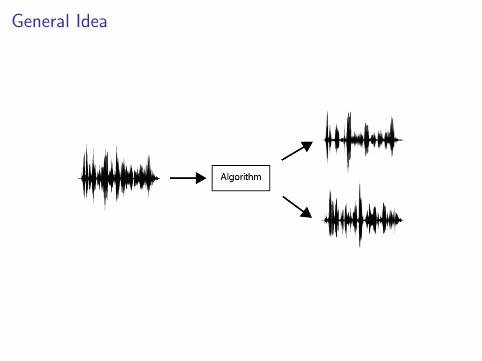
General Idea

Music Remixing and Content Creation
Music remixing and content creation
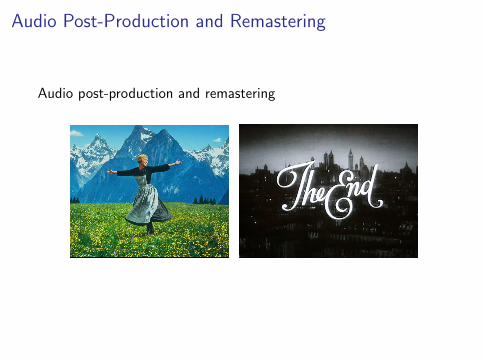
Audio Post-Production and Remastering
Audio post-production and remastering

Spatial Audio and Upmixing
Spatial audio and upmixing
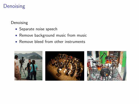
Denoising
Denoising
• Separate noise speech
• Remove background music from music
• Remove bleed from other instruments

Roadmap of Talk
1 Motivation
2 Current Approaches
3 Non-Negative Matrix Factorization (NMF)
4 Source Separation via NMF
5 Algorithms for NMF
6 Matlab Code
Current Approaches I
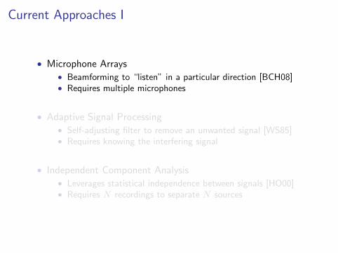
• Microphone Arrays• Beamforming to “listen” in a particular direction [BCH08]• Requires multiple microphones
• Adaptive Signal Processing• Self-adjusting filter to remove an unwanted signal [WS85]• Requires knowing the interfering signal
• Independent Component Analysis• Leverages statistical independence between signals [HO00]• Requires N recordings to separate N sources

Current Approaches I
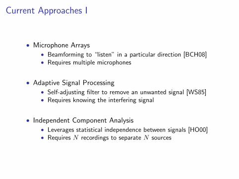
• Microphone Arrays• Beamforming to “listen” in a particular direction [BCH08]• Requires multiple microphones
• Adaptive Signal Processing• Self-adjusting filter to remove an unwanted signal [WS85]• Requires knowing the interfering signal
• Independent Component Analysis• Leverages statistical independence between signals [HO00]• Requires N recordings to separate N sources
Current Approaches I
• Microphone Arrays• Beamforming to “listen” in a particular direction [BCH08]• Requires multiple microphones
• Adaptive Signal Processing• Self-adjusting filter to remove an unwanted signal [WS85]• Requires knowing the interfering signal
• Independent Component Analysis• Leverages statistical independence between signals [HO00]• Requires N recordings to separate N sources

Current Approaches II
• Computational Auditory Scene Analysis• Leverages knowledge of auditory system [WB06]• Still requires some other underlying algorithm
• Sinusoidal Modeling• Decomposes sound into sinusoidal peak tracks [Smi11, Wan94]• Problem in assigning sound source to peak tracks
• Classical Denoising and Enhancement• Wiener filtering, spectral subtraction, MMSE STSA (Talk 1)• Difficulty with time varying noise
Current Approaches II
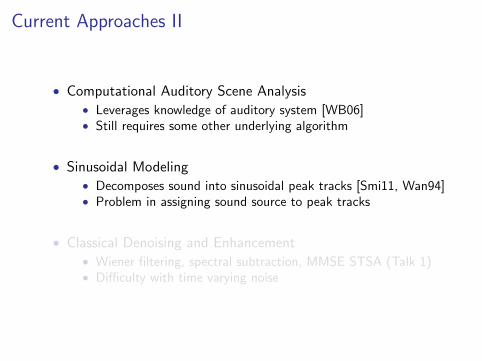
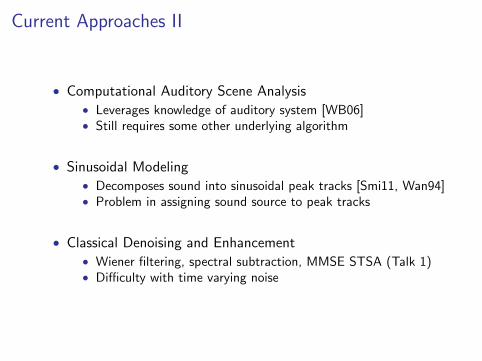
• Computational Auditory Scene Analysis• Leverages knowledge of auditory system [WB06]• Still requires some other underlying algorithm
• Sinusoidal Modeling• Decomposes sound into sinusoidal peak tracks [Smi11, Wan94]• Problem in assigning sound source to peak tracks
• Classical Denoising and Enhancement• Wiener filtering, spectral subtraction, MMSE STSA (Talk 1)• Difficulty with time varying noise

Current Approaches III
• Non-Negative Matrix Factorization & Probabilistic Models• Popular technique for processing audio, image, text, etc.• Models spectrogram data as mixture of prototypical spectra• Relatively compact and easy to code algorithms• Amenable to machine learning• In many cases, works surprisingly well• The topic of today’s discussion!

Roadmap of Talk
1 Motivation
2 Current Approaches
3 Non-Negative Matrix Factorization (NMF)
4 Source Separation via NMF
5 Algorithms for NMF
6 Matlab Code
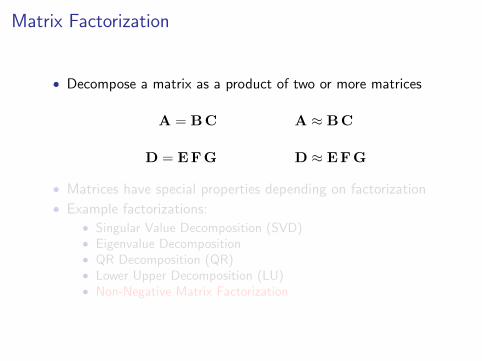
Matrix Factorization
• Decompose a matrix as a product of two or more matrices
A = BC A ≈ BC
D = EFG D ≈ EFG
• Matrices have special properties depending on factorization
• Example factorizations:• Singular Value Decomposition (SVD)• Eigenvalue Decomposition• QR Decomposition (QR)• Lower Upper Decomposition (LU)• Non-Negative Matrix Factorization

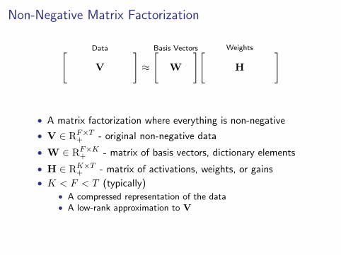
Non-Negative Matrix Factorization
Data[V
]≈
Basis Vectors[W
] Weights[H
]
• A matrix factorization where everything is non-negative
• V ∈ RF×T+ - original non-negative data
• W ∈ RF×K+ - matrix of basis vectors, dictionary elements
• H ∈ RK×T+ - matrix of activations, weights, or gains
• K < F < T (typically)• A compressed representation of the data• A low-rank approximation to V

Interpretation of V
Data[V
]≈
Basis Vectors[W
] Weights[H
]
• V ∈ RF×T+ - original non-negative data• Each column is an F-dimensional data sample• Each row represents a data feature• We will use audio spectrogram data as V

Interpretation of W
Data[V
]≈
Basis Vectors[W
] Weights[H
]
• W ∈ RF×K+ - matrix of basis vectors, dictionary elements• A single column is referred to as a basis vector• Not orthonormal, but commonly normalized to one

Interpretation of H
Data[V
]≈
Basis Vectors[W
] Weights[H
]
• H ∈ RK×T+ - matrix of activations, weights, or gains• A row represents the gain of corresponding basis vector• Not orthonormal, but commonly normalized to one

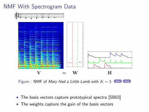
NMF With Spectrogram Data
V ≈ W H
Figure : NMF of Mary Had a Little Lamb with K = 3 play stop
• The basis vectors capture prototypical spectra [SB03]
• The weights capture the gain of the basis vectors
NMF With Spectrogram Data
V ≈ W H
Figure : NMF of Mary Had a Little Lamb with K = 3 play stop
• The basis vectors capture prototypical spectra [SB03]
• The weights capture the gain of the basis vectors

Factorization Interpretation I
Columns of V ≈ as a weighted sum (mixture) of basis vectors
v1 v2 ... vT
≈ K∑j=1
Hj1 wj
K∑j=1
Hj2 wj ...K∑j=1
HjT wj

Factorization Interpretation II
V is approximated as sum of matrix “layers”
= + +
v1 v2 . . . vT
≈w1 w2 . . . wK
hT
1
hT
2...
hT
K
V ≈ w1 h
T1 +w2 h
T2 + . . .+wK hT
K

Questions
• How do we use W and H to perform separation?
• How do we solve for W and H, given a known V?

Questions
• How do we use W and H to perform separation?
• How do we solve for W and H, given a known V?
Roadmap of Talk
1 Motivation
2 Current Approaches
3 Non-Negative Matrix Factorization (NMF)
4 Source Separation via NMF
5 Algorithms for NMF
6 Matlab Code
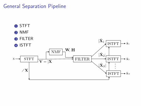
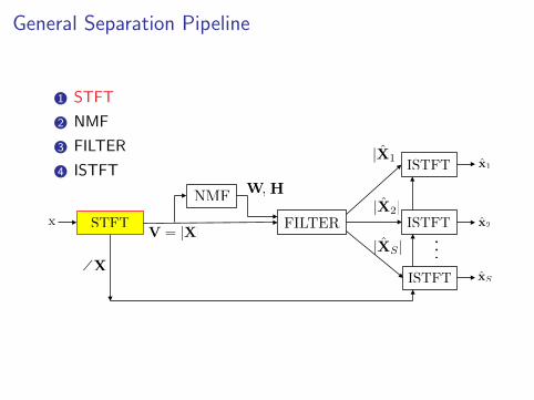
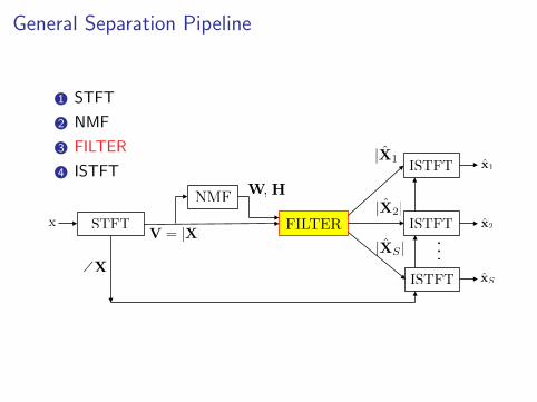
General Separation Pipeline
1 STFT
2 NMF
3 FILTER
4 ISTFT
NMF
STFT
ISTFT
FILTERx
\XxS
x1
x2ISTFT
ISTFT
...
W H,
|X1|
|X2|
|XS |V = |X|
General Separation Pipeline
1 STFT
2 NMF
3 FILTER
4 ISTFT
NMF
STFT
ISTFT
FILTERx
\XxS
x1
x2ISTFT
ISTFT
...
W H,
|X1|
|X2|
|XS |V = |X|
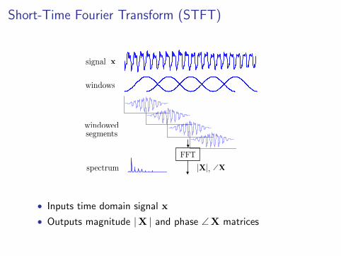
Short-Time Fourier Transform (STFT)
x
FFT
signal
windows
windowedsegments
spectrum |X| \X,
• Inputs time domain signal x
• Outputs magnitude |X | and phase ∠X matrices
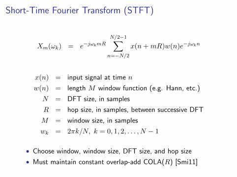
Short-Time Fourier Transform (STFT)
Xm(ωk) = e−jωkmR
N/2−1∑n=−N/2
x(n+mR)w(n)e−jωkn
x(n) = input signal at time n
w(n) = length M window function (e.g. Hann, etc.)
N = DFT size, in samples
R = hop size, in samples, between successive DFT
M = window size, in samples
wk = 2πk/N, k = 0, 1, 2, . . . , N − 1
• Choose window, window size, DFT size, and hop size
• Must maintain constant overlap-add COLA(R) [Smi11]

General Separation Pipeline
1 STFT
2 NMF
3 FILTER
4 ISTFT
NMF
STFT
ISTFT
FILTERx
\XxS
x1
x2ISTFT
ISTFT
...
W H,
|X1|
|X2|
|XS |V = |X|
Non-Negative Matrix Factorization
• Inputs |X |, outputs W and H
• Algorithm to be discussed
General Separation Pipeline
1 STFT
2 NMF
3 FILTER
4 ISTFT
NMF
STFT
ISTFT
FILTERx
\XxS
x1
x2ISTFT
ISTFT
...
W H,
|X1|
|X2|
|XS |V = |X|

Source Synthesis I
• Choose a subset of basis vectors Ws and activations Hs toreconstruct source s
• Estimate the source s magnitude:
|Xs| = WsHs =∑i∈s
(wi hTi )

Source Synthesis I
• Choose a subset of basis vectors Ws and activations Hs toreconstruct source s
• Estimate the source s magnitude:
|Xs| = WsHs =∑i∈s
(wi hTi )

Source Synthesis II
Example 1: “D” pitches as a single source
= + +
V ≈ w1 hT1 +w2 h
T2 +w3 h
T3
• |Xs| ≈ w1 hT1
• Use one basis vector to reconstruct a source

Source Synthesis III
Example 2: “D” and “E” pitches as a source
= + +
V ≈ w1 hT1 +w2 h
T2 +w3 h
T3
• |Xs| ≈ w1 hT1 +w2 h
T2
• Use two (or more) basis vector to reconstruct a source

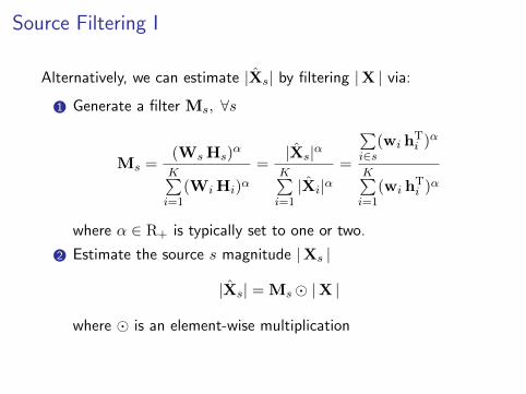
Source Filtering I
Alternatively, we can estimate |Xs| by filtering |X | via:
1 Generate a filter Ms, ∀s
Ms =(WsHs)
α
K∑i=1
(WiHi)α=|Xs|αK∑i=1|Xi|α
=
∑i∈s
(wi hTi )α
K∑i=1
(wi hTi )α
where α ∈ R+ is typically set to one or two.
2 Estimate the source s magnitude |Xs |
|Xs| = Ms� |X |
where � is an element-wise multiplication

Source Filtering II
Example: Choose “D” pitches as a single source w/one basis vector
1 Compute filter Ms =w1 h
T1
K∑i=1
wi hTi
, with α = 1
= / ( + + )
2 Multiply with |Xs| = Ms� |X |
= �

Source Filtering III
• The filter M is referred to as a masking filter or soft mask
• Tends to perform better than the reconstruction method
• Similar to Wiener filtering discussed in Talk 1

General Separation Pipeline
1 STFT
2 NMF
3 FILTER
4 ISTFT
NMF
STFT
ISTFT
FILTERx
\XxS
x1
x2ISTFT
ISTFT
...
W H,
|X1|
|X2|
|XS |V = |X|
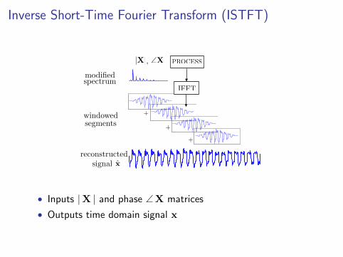
Inverse Short-Time Fourier Transform (ISTFT)
PROCESS
IFFT
+
+
+
modifiedspectrum
windowedsegments
reconstructedsignal
|X| \X,
x
• Inputs |X | and phase ∠X matrices
• Outputs time domain signal x

General Separation Pipeline
1 STFT
2 NMF
3 FILTER
4 ISTFT
NMF
STFT
ISTFT
FILTERx
\XxS
x1
x2ISTFT
ISTFT
...
W H,
|X1|
|X2|
|XS |V = |X|
Roadmap of Talk
1 Motivation
2 Current Approaches
3 Non-Negative Matrix Factorization (NMF)
4 Source Separation via NMF
5 Algorithms for NMF
6 Matlab Code

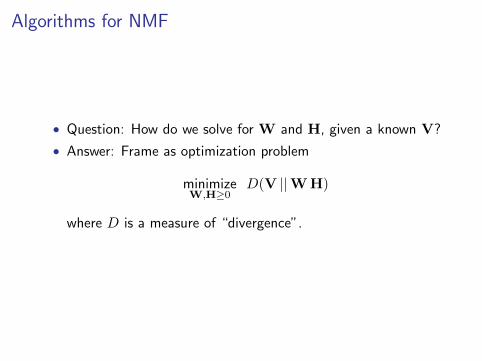
Algorithms for NMF
• Question: How do we solve for W and H, given a known V?
• Answer: Frame as optimization problem
minimizeW,H≥0
D(V ||WH)
where D is a measure of “divergence”.
Algorithms for NMF
• Question: How do we solve for W and H, given a known V?
• Answer: Frame as optimization problem
minimizeW,H≥0
D(V ||WH)
where D is a measure of “divergence”.

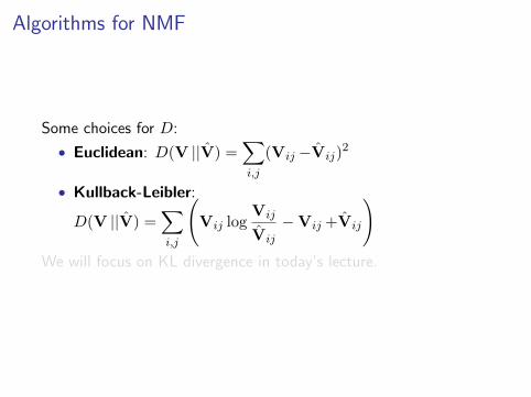
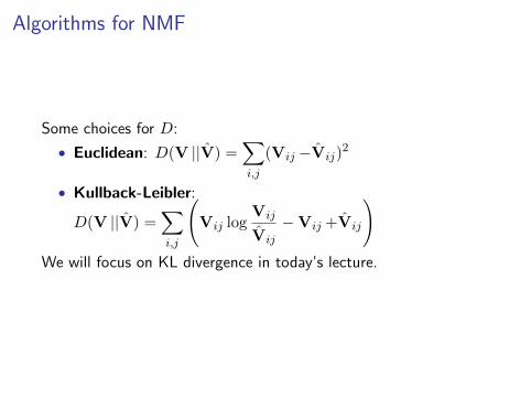
Algorithms for NMF
Some choices for D:
• Euclidean: D(V ||V) =∑i,j
(Vij −Vij)2
• Kullback-Leibler:
D(V ||V) =∑i,j
(Vij log
Vij
Vij
−Vij +Vij
)We will focus on KL divergence in today’s lecture.
Algorithms for NMF
Some choices for D:
• Euclidean: D(V ||V) =∑i,j
(Vij −Vij)2
• Kullback-Leibler:
D(V ||V) =∑i,j
(Vij log
Vij
Vij
−Vij +Vij
)We will focus on KL divergence in today’s lecture.
Algorithms for NMF
Some choices for D:
• Euclidean: D(V ||V) =∑i,j
(Vij −Vij)2
• Kullback-Leibler:
D(V ||V) =∑i,j
(Vij log
Vij
Vij
−Vij +Vij
)We will focus on KL divergence in today’s lecture.

Geometric View of NMF

Algorithms for NMF
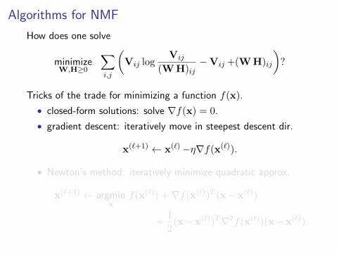
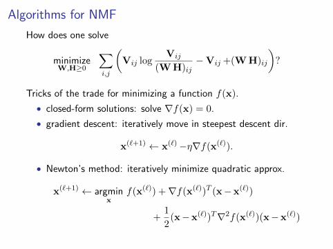
How does one solve
minimizeW,H≥0
∑i,j
(Vij log
Vij
(WH)ij−Vij +(WH)ij
)?
Tricks of the trade for minimizing a function f(x).
• closed-form solutions: solve ∇f(x) = 0.
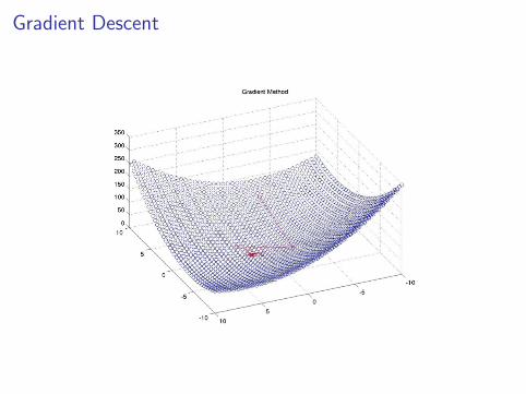
• gradient descent: iteratively move in steepest descent dir.
x(`+1) ← x(`)−η∇f(x(`)).
• Newton’s method: iteratively minimize quadratic approx.
x(`+1) ← argminx
f(x(`)) +∇f(x(`))T (x−x(`))
+1
2(x−x(`))T∇2f(x(`))(x−x(`))

Algorithms for NMF
How does one solve
minimizeW,H≥0
∑i,j
(Vij log
Vij
(WH)ij−Vij +(WH)ij
)?
Tricks of the trade for minimizing a function f(x).
• closed-form solutions: solve ∇f(x) = 0.
• gradient descent: iteratively move in steepest descent dir.
x(`+1) ← x(`)−η∇f(x(`)).
• Newton’s method: iteratively minimize quadratic approx.
x(`+1) ← argminx
f(x(`)) +∇f(x(`))T (x−x(`))
+1
2(x−x(`))T∇2f(x(`))(x−x(`))
Gradient Descent

Newton’s Method

Meta Algorithms
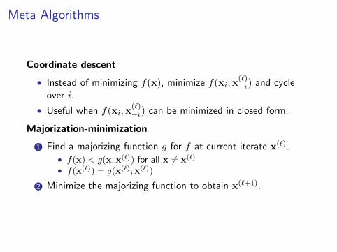
Coordinate descent
• Instead of minimizing f(x), minimize f(xi;x(`)−i) and cycle
over i.
• Useful when f(xi;x(`)−i) can be minimized in closed form.
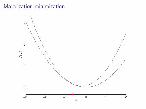
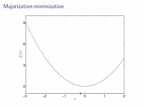
Majorization-minimization
1 Find a majorizing function g for f at current iterate x(`).• f(x) < g(x;x(`)) for all x 6= x(`)
• f(x(`)) = g(x(`);x(`))
2 Minimize the majorizing function to obtain x(`+1).

Meta Algorithms
Coordinate descent
• Instead of minimizing f(x), minimize f(xi;x(`)−i) and cycle
over i.
• Useful when f(xi;x(`)−i) can be minimized in closed form.
Majorization-minimization
1 Find a majorizing function g for f at current iterate x(`).• f(x) < g(x;x(`)) for all x 6= x(`)
• f(x(`)) = g(x(`);x(`))
2 Minimize the majorizing function to obtain x(`+1).

Majorization-minimization
−3 −2 −1 0 1 2
0
3
6
9
x
f(x
)

Majorization-minimization
−3 −2 −1 0 1 2
0
3
6
9
x
f(x
)

Majorization-minimization
−3 −2 −1 0 1 2
0
3
6
9
x
f(x
)

Majorization-minimization
−3 −2 −1 0 1 2
0
3
6
9
x
f(x
)
Majorization-minimization
−3 −2 −1 0 1 2
0
3
6
9
x
f(x
)

Majorization-minimization
−3 −2 −1 0 1 2
0
3
6
9
x
f(x
)
Majorization-minimization
−3 −2 −1 0 1 2
0
3
6
9
x
f(x
)
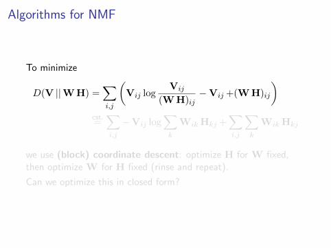
Algorithms for NMF
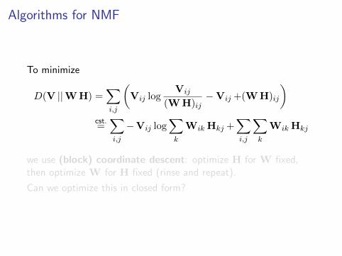
To minimize
D(V ||WH) =∑i,j
(Vij log
Vij
(WH)ij−Vij +(WH)ij
)cst.=∑i,j
−Vij log∑k
WikHkj +∑i,j
∑k
WikHkj
we use (block) coordinate descent: optimize H for W fixed,then optimize W for H fixed (rinse and repeat).
Can we optimize this in closed form?
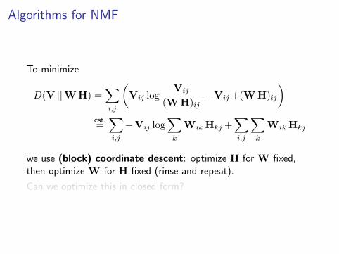
Algorithms for NMF
To minimize
D(V ||WH) =∑i,j
(Vij log
Vij
(WH)ij−Vij +(WH)ij
)cst.=∑i,j
−Vij log∑k
WikHkj +∑i,j
∑k
WikHkj
we use (block) coordinate descent: optimize H for W fixed,then optimize W for H fixed (rinse and repeat).
Can we optimize this in closed form?
Algorithms for NMF
To minimize
D(V ||WH) =∑i,j
(Vij log
Vij
(WH)ij−Vij +(WH)ij
)cst.=∑i,j
−Vij log∑k
WikHkj +∑i,j
∑k
WikHkj
we use (block) coordinate descent: optimize H for W fixed,then optimize W for H fixed (rinse and repeat).
Can we optimize this in closed form?

Algorithms for NMF
To minimize
D(V ||WH) =∑i,j
(Vij log
Vij
(WH)ij−Vij +(WH)ij
)cst.=∑i,j
−Vij log∑k
WikHkj +∑i,j
∑k
WikHkj
we use (block) coordinate descent: optimize H for W fixed,then optimize W for H fixed (rinse and repeat).
Can we optimize this in closed form?
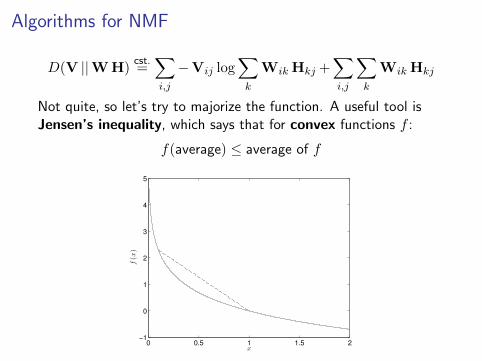
Algorithms for NMF
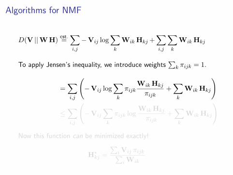
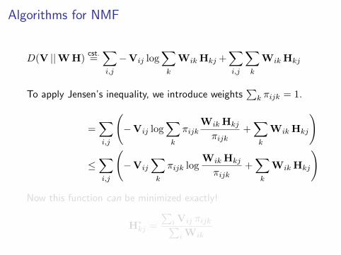
D(V ||WH)cst.=∑i,j
−Vij log∑k
WikHkj +∑i,j
∑k
WikHkj
Not quite, so let’s try to majorize the function. A useful tool isJensen’s inequality, which says that for convex functions f :
f(average) ≤ average of f
0 0.5 1 1.5 2−1
0
1
2
3
4
5
x
f(x
)
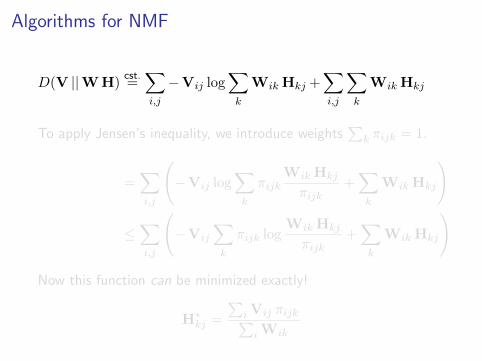
Algorithms for NMF
D(V ||WH)cst.=∑i,j
−Vij log∑k
WikHkj +∑i,j
∑k
WikHkj
To apply Jensen’s inequality, we introduce weights∑
k πijk = 1.
=∑i,j
(−Vij log
∑k
πijkWikHkj
πijk+∑k
WikHkj
)
≤∑i,j
(−Vij
∑k
πijk logWikHkj
πijk+∑k
WikHkj
)
Now this function can be minimized exactly!
H∗kj =
∑iVij πijk∑iWik
Algorithms for NMF
D(V ||WH)cst.=∑i,j
−Vij log∑k
WikHkj +∑i,j
∑k
WikHkj
To apply Jensen’s inequality, we introduce weights∑
k πijk = 1.
=∑i,j
(−Vij log
∑k
πijkWikHkj
πijk+∑k
WikHkj
)
≤∑i,j
(−Vij
∑k
πijk logWikHkj
πijk+∑k
WikHkj
)
Now this function can be minimized exactly!
H∗kj =
∑iVij πijk∑iWik
Algorithms for NMF
D(V ||WH)cst.=∑i,j
−Vij log∑k
WikHkj +∑i,j
∑k
WikHkj
To apply Jensen’s inequality, we introduce weights∑
k πijk = 1.
=∑i,j
(−Vij log
∑k
πijkWikHkj
πijk+∑k
WikHkj
)
≤∑i,j
(−Vij
∑k
πijk logWikHkj
πijk+∑k
WikHkj
)
Now this function can be minimized exactly!
H∗kj =
∑iVij πijk∑iWik

Algorithms for NMF
D(V ||WH)cst.=∑i,j
−Vij log∑k
WikHkj +∑i,j
∑k
WikHkj
To apply Jensen’s inequality, we introduce weights∑
k πijk = 1.
=∑i,j
(−Vij log
∑k
πijkWikHkj
πijk+∑k
WikHkj
)
≤∑i,j
(−Vij
∑k
πijk logWikHkj
πijk+∑k
WikHkj
)
Now this function can be minimized exactly!
H∗kj =
∑iVij πijk∑iWik
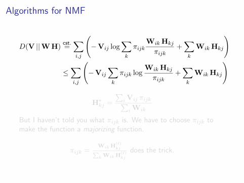
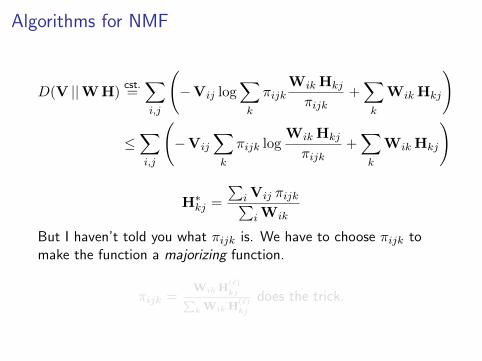
Algorithms for NMF
D(V ||WH)cst.=∑i,j
(−Vij log
∑k
πijkWikHkj
πijk+∑k
WikHkj
)
≤∑i,j
(−Vij
∑k
πijk logWikHkj
πijk+∑k
WikHkj
)
H∗kj =
∑iVij πijk∑iWik
But I haven’t told you what πijk is. We have to choose πijk tomake the function a majorizing function.
πijk =Wik H
(`)kj∑
k Wik H(`)kj
does the trick.

Algorithms for NMF
D(V ||WH)cst.=∑i,j
(−Vij log
∑k
πijkWikHkj
πijk+∑k
WikHkj
)
≤∑i,j
(−Vij
∑k
πijk logWikHkj
πijk+∑k
WikHkj
)
H∗kj =
∑iVij πijk∑iWik
But I haven’t told you what πijk is. We have to choose πijk tomake the function a majorizing function.
πijk =Wik H
(`)kj∑
k Wik H(`)kj
does the trick.
Algorithms for NMF
D(V ||WH)cst.=∑i,j
(−Vij log
∑k
πijkWikHkj
πijk+∑k
WikHkj
)
≤∑i,j
(−Vij
∑k
πijk logWikHkj
πijk+∑k
WikHkj
)
H∗kj =
∑iVij πijk∑iWik
But I haven’t told you what πijk is. We have to choose πijk tomake the function a majorizing function.
πijk =Wik H
(`)kj∑
k Wik H(`)kj
does the trick.

Algorithms for NMF
D(V ||WH)cst.=∑i,j
(−Vij log
∑k
πijkWikHkj
πijk+∑k
WikHkj
)
≤∑i,j
(−Vij
∑k
πijk logWikHkj
πijk+∑k
WikHkj
)
H∗kj =
∑iVij πijk∑iWik
But I haven’t told you what πijk is. We have to choose πijk tomake the function a majorizing function.
πijk =Wik H
(`)kj∑
k Wik H(`)kj
does the trick.

Algorithms for NMF
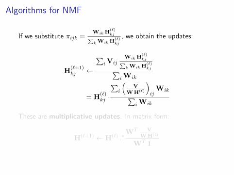
If we substitute πijk =Wik H
(`)kj∑
k Wik H(`)kj
, we obtain the updates:
H(`+1)kj ←
∑iVij
Wik H(`)kj∑
k Wik H(`)kj∑
iWik
= H(`)kj ·
∑i
(V
WH(`)
)ijWik∑
iWik
These are multiplicative updates. In matrix form:
H(`+1) ← H(`) .∗WT V
WH(`)
WT 1

Algorithms for NMF
If we substitute πijk =Wik H
(`)kj∑
k Wik H(`)kj
, we obtain the updates:
H(`+1)kj ←
∑iVij
Wik H(`)kj∑
k Wik H(`)kj∑
iWik
= H(`)kj ·
∑i
(V
WH(`)
)ijWik∑
iWik
These are multiplicative updates. In matrix form:
H(`+1) ← H(`) .∗WT V
WH(`)
WT 1
Algorithms for NMF
If we substitute πijk =Wik H
(`)kj∑
k Wik H(`)kj
, we obtain the updates:
H(`+1)kj ←
∑iVij
Wik H(`)kj∑
k Wik H(`)kj∑
iWik
= H(`)kj ·
∑i
(V
WH(`)
)ijWik∑
iWik
These are multiplicative updates. In matrix form:
H(`+1) ← H(`) .∗WT V
WH(`)
WT 1

Algorithms for NMF
If we substitute πijk =Wik H
(`)kj∑
k Wik H(`)kj
, we obtain the updates:
H(`+1)kj ←
∑iVij
Wik H(`)kj∑
k Wik H(`)kj∑
iWik
= H(`)kj ·
∑i
(V
WH(`)
)ijWik∑
iWik
These are multiplicative updates. In matrix form:
H(`+1) ← H(`) .∗WT V
WH(`)
WT 1
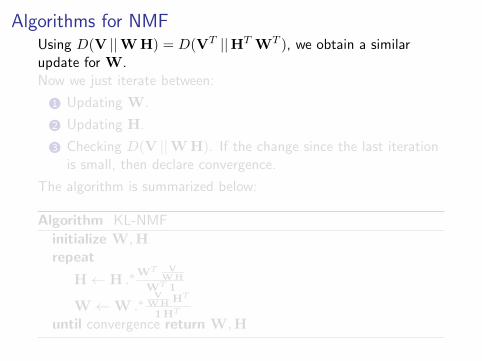
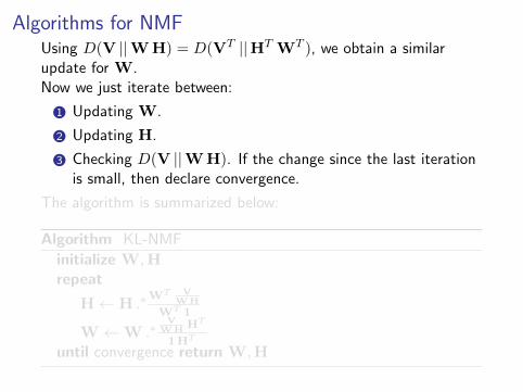
Algorithms for NMFUsing D(V ||WH) = D(VT ||HT WT ), we obtain a similarupdate for W.Now we just iterate between:
1 Updating W.
2 Updating H.
3 Checking D(V ||WH). If the change since the last iterationis small, then declare convergence.
The algorithm is summarized below:
Algorithm KL-NMF
initialize W,Hrepeat
H← H .∗WT V
WH
WT 1
W←W .∗V
WHHT
1HT
until convergence return W,H
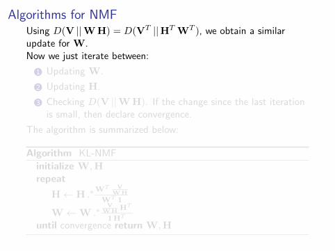
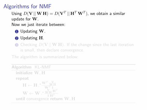

Caveats
• The NMF problem is non-convex.
−2 −1 0 1 2 3 4 5−15
−10
−5
0
5
10
15
20
25
30
• The algorithm is only guaranteed to find a local optimum.
• The algorithm is sensitive to choice of initialization.

Roadmap of Talk
1 Motivation
2 Current Approaches
3 Non-Negative Matrix Factorization (NMF)
4 Source Separation via NMF
5 Algorithms for NMF
6 Matlab Code

STFT
FFTSIZE = 1024;
HOPSIZE = 256;
WINDOWSIZE = 512;
X = myspectrogram(x,FFTSIZE,fs,hann(WINDOWSIZE),-HOPSIZE);
V = abs(X(1:(FFTSIZE/2+1),:));
F = size(V,1);
T = size(V,2);
• https://ccrma.stanford.edu/~jos/sasp/Matlab_
listing_myspectrogram_m.html
• https://ccrma.stanford.edu/~jos/sasp/Matlab_
listing_invmyspectrogram_m.html
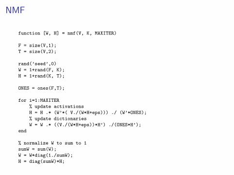
NMF
function [W, H] = nmf(V, K, MAXITER)
F = size(V,1);
T = size(V,2);
rand(’seed’,0)
W = 1+rand(F, K);
H = 1+rand(K, T);
ONES = ones(F,T);
for i=1:MAXITER
% update activations
H = H .* (W’*( V./(W*H+eps))) ./ (W’*ONES);
% update dictionaries
W = W .* ((V./(W*H+eps))*H’) ./(ONES*H’);
end
% normalize W to sum to 1
sumW = sum(W);
W = W*diag(1./sumW);
H = diag(sumW)*H;
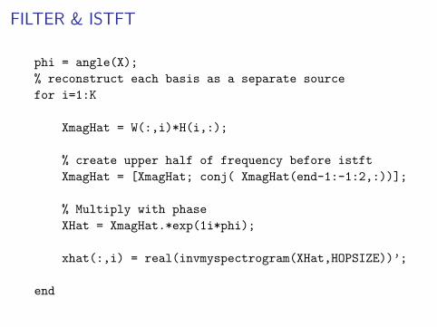
FILTER & ISTFT
phi = angle(X);
% reconstruct each basis as a separate source
for i=1:K
XmagHat = W(:,i)*H(i,:);
% create upper half of frequency before istft
XmagHat = [XmagHat; conj( XmagHat(end-1:-1:2,:))];
% Multiply with phase
XHat = XmagHat.*exp(1i*phi);
xhat(:,i) = real(invmyspectrogram(XHat,HOPSIZE))’;
end
References I
Jacob Benesty, Jingdong Chen, and Yiteng Huang,Microphone array signal processing, Springer, 2008.
C. Fevotte, N. Bertin, and J.-L. Durrieu, Nonnegative matrixfactorization with the itakura-saito divergence: Withapplication to music analysis, Neural Computation 21 (2009),no. 3, 793–830.
C. Fevotte and J. Idier, Algorithms for nonnegative matrixfactorization with the β-divergence, Neural Computation 23(2011), no. 9, 2421–2456.
A. Hyvarinen and E. Oja, Independent component analysis:algorithms and applications, Neural Netw. 13 (2000), no. 4-5,411–430.
D. D. Lee and H. S. Seung, Algorithms for non-negativematrix factorization, Advances in Neural InformationProcessing Systems (NIPS), MIT Press, 2001, pp. 556–562.
References II
P. Smaragdis and J.C. Brown, Non-negative matrixfactorization for polyphonic music transcription, IEEEWorkshop on Applications of Signal Processing to Audio andAcoustics (WASPAA), oct. 2003, pp. 177 – 180.
J. O. Smith, Spectral audio signal processing,http://ccrma.stanford.edu/~jos/sasp/, 2011, onlinebook.
Avery Li-chun Wang, Instantaneous and frequency-warpedsignal processing techniques for auditory source separation,Ph.D. thesis, Stanford University, 1994.
DeLiang Wang and Guy J. Brown, Computational auditoryscene analysis: Principles, algorithms, and applications,Wiley-IEEE Press, 2006.

References III
Bernard Widrow and Samuel D. Stearns, Adaptive signalprocessing, Prentice-Hall, Inc., Upper Saddle River, NJ, USA,1985.