Sound collection and visualization system enabledparticipatory and opportunistic sensing approaches

Sunao Hara, Masanobu AbeGraduate School of Natural Science and Technology

Okayama UniversityOkayama, Japan 700–8350

Email: hara@okayama-u.ac.jp, abe@cs.okayama-u.ac.jp

Noboru SoneharaNational Institute of Informatics

Tokyo, Japan 101-8430Email: sonehara@nii.ac.jp

Abstract—This paper presents a sound collection system tovisualize environmental sounds that are collected using a crowd-sourcing approach. An analysis of physical features is generallyused to analyze sound properties; however, human beings notonly analyze but also emotionally connect to sounds. If we want tovisualize the sounds according to the characteristics of the listener,we need to collect not only the raw sound, but also the subjectivefeelings associated with them. For this purpose, we developeda sound collection system using a crowdsourcing approach tocollect physical sounds, their statistics, and subjective evaluationssimultaneously. We then conducted a sound collection experimentusing the developed system on ten participants. We collected 6,257samples of equivalent loudness levels and their locations, and 516samples of sounds and their locations. Subjective evaluations bythe participants are also included in the data. Next, we tried tovisualize the sound on a map. The loudness levels are visualizedas a color map and the sounds are visualized as icons whichindicate the sound type. Finally, we conducted a discriminationexperiment on the sound to implement a function of automaticconversion from sounds to appropriate icons. The classifier istrained on the basis of the GMM-UBM (Gaussian Mixture Modeland Universal Background Model) method. Experimental resultsshow that the F-measure is 0.52 and the AUC is 0.79.

I. INTRODUCTION

Sound is one of the most important information sources forhuman beings for understanding the environment around them.However, humans interpret sounds differently on the basis oftheir experiences and their current situation. In this study, werefer to such a sound as an environmental sound. For example,we may feel a sound is louder at night than at noon even ifit is the same sound. Take another example, the cry of aninfant might be felt differently by a listener who has a child,or younger sisters or brothers compared with someone whodoes not. Therefore, to understand environmental sounds inthe real world, we need to consider contextual information,i.e., not only sound properties, but also the situation of thelistener.

Many methods for sound interpretation are known, but theyonly provide a general interpretation of sounds. Sound proper-ties are generally interpreted as having spectral and/or temporalparameters, such as spectrum, fundamental frequency, andloudness. On the basis of a perceptual point of view, severalmethods have been introduced to interpret sound propertiessuch as critical-band analysis, octave-bandpass analysis, andA-weighting filtering. However, these methods only interpret

the sound properties on the basis of a common understandingof human beings, but this is insufficient.

In this study, we developed a sound collection methodapplying crowdsourcing approaches in order to understandenvironmental sounds by considering contextual information.The sound collection is performed by one application on asmart device. The collected data fall into two types; one isuser-specific and the other is statistical data. We apply twoparadigms of crowdsourcing to collect the sounds; i.e., partic-ipatory sensing [1], [2] and opportunistic sensing [3]. Usingthe participatory sensing paradigm, we can collect sounds thatparticipants are interested in or appreciate, therefore we appliedthis paradigm for collecting the raw waveform of sounds.Conversely, using the opportunistic sensing paradigm, we cancollect sound statistics and, in particular, collect the loudnesslevel as statistics in this paper.

The data should be statistically processed or anonymizedto reduce any privacy risk. From this perspective, EarPhone [4]and NoiseTube [5] are important existing works. In these stud-ies, they tried to collect environmental sounds as noise usinga crowdsourcing approach; in other words, they mainly dealtwith the statistics of the sound. McGraw et al. [6] collectedsound data using Amazon Mechanical Turk as a crowdsourcingplatform. Matsuyama et al. [7] conducted their sound-datacollection using an HTML5 application and evaluated theperformance of sound classifiers. Their study mainly deals withthe raw waveform of sounds that cannot identify the listener.In contrast with these studies, the main contribution of ourpaper is to enable sound-data collection that takes contextualinformation into account.

We developed a visualization method for the sounds col-lected by participatory and opportunistic sensing paradigms.This visualization is one of the most important processes forthe interpretation of environmental sounds. The waveforms ofthe sound are visualized by icons symbolizing the sounds at acertain location on a map, and the statistics of the sounds arevisualized as colors on the same map.

Section II presents a summary of the sound collectionsystem and Section III explains a sound collection experiment,using the system developed in Section II. Section IV presentsthe visualization method for sound mapping using the collecteddata and Section V explains an experiment to discriminatethe sound type for evaluating the possibility of automaticclassification of the sound collected in a real environment.

CORE Metadata, citation and similar papers at core.ac.uk

Provided by Okayama University Scientific Achievement Repository

II. DEVELOPMENT OF SOUND COLLECTION SYSTEM

A. Recording application for environmental sound

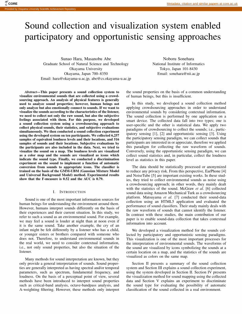
We developed a recording application for environmentalsound. We used a Google Nexus 7, which is a 7-inch touchscreen tablet for Android OS. Figures 1a and 1b show screenshots of the location logging and sound logging screens,respectively. Data recorded is starts working when the userslides the button at the upper side of the screen.

On the location logging screen, the system can recordhighly accurate location information using GPS, Cell-ID, orWi-Fi networks via the Android API. The default samplingrate is one second, but this can be changed by the user throughthe settings. A map on the screen can show the history of thelocations of the user as pin icons on the map.

On the sound logging screen, the system can record rawsound signals and calculate loudness levels using a microphoneon the device. It always stores the sound data of the most recenttwenty seconds using a ring buffer and also analyzes the soundto calculate the equivalent loudness level and levels of an 8-channel frequency filterbank at intervals of one second.

Annotations on the sound can be attached during therecording by users, such as subjective evaluation, sound typeselection, and free description. The subjective evaluation hasa five-grade scale for two metrics; one is subjective loudnesslevel and the other is subjective crowdedness level. The soundtype is easy to annotate with a selection of five preset soundtypes. A free description can be used as a summary of therecording environment, feelings, etc.

All of the annotations are recorded in log files with timeinformation and a WAV file, including ten seconds of sound,is created at the same time. These can be sent to a server ifthe application settings permit. The sent log files are parsed onthe server and they are shown in a timeline view like that ofTwitter, which is shared for all users in this implementation.

(a) Location logging screen (b) Sound logging screen

Fig. 1. Screenshots of the recording application

B. Specification of the data collected by the application

The application generates sound files and three types oflog file in one session. The log files are a location history log-file, loudness level log-file, and tweet log-file and they containtime information, which is triggered. In this paper, we use theSystem.currentTimeMillis() method of standard Java API fortime synchronization of files because of its simplicity.

Sounds are recorded at a sampling frequency of 32000Hz and 16-bits per second with a single channel. They areanalyzed at equivalent loudness level Leq per second,

Leq = 10 log101

N

N∑n=1

(A · s[n])2 , (1)

where s[n] is a sampled signal, A is a transform factor fromsampled amplitude to sound pressure level, and N is the signallength. In this paper, N is fixed to 32000, which is equivalentto 1 s. A is detected by a preliminary examination to comparewith values of a sound level meter, RION NL–42. The lowerlimit of loudness level by the application on the Nexus 7 isapproximately 40 dB(FLAT) because of the performance ofthe device’s A/D equipment.

Addition to Leq , this system can also record filterbank output levels in 8-channel, which is related to octaveband filter analysis. The filter is implemented using trianglewindows. The central frequencies of the filter are fc =[63, 125, 250, 500, 1000, 2000, 4000, 8000].

C. Server application for collection and exploration of thesounds

The client and server applications communicate via HTTPprotocols. The server implements APIs for receiving andbrowsing data and the browsing API can create not only ageneral HTML view for WWW browsers, but also a JSON(JavaScript Object Notation) view for advanced applications.

The server system includes several open-source softwares.The server OS is a Debian GNU/Linux 7.5 (Wheezy) as avirtual machine on VMware ESXi 5.1. The web applicationframework is Mojolicious 1 with Perl language. The back-enddatabase software is MongoDB 2. The application is runningon Mojo::Server::Hyptonotoad 3 with an nginx front-end server4. The system will be used for the crowd-sourced soundrecordings, hence, a large number of users will use the system,and hence it must have the appropriate processing capacity.These software have a distributed computing architecture thatmight be an answer to the problems of heavy usage.

III. LOUDNESS AND ENVIRONMENTAL SOUNDS DATACOLLECTION

A. Conditions of data collection

A data collection experiment was conducted on ten par-ticipants comprising two faculty members and eight graduatestudents, who commute to Okayama University to work. The

1http://mojolicio.us/2http://www.mongodb.org/3http://mojolicio.us/perldoc/Mojo/Server/Hypnotoad4http://nginx.org/

participants were instructed how to use smart devices and thedata collection applications. They were asked to collect thesounds, annotations, and loudness levels during travel to andfrom work. Some were also asked to collect data near theirhome or railway stations.

They recorded loudness levels during application runningand the sound with the annotations at various intervals byuser. Data collection was expected to be conducted by theparticipants holding the devices in their hands during datacollection because of the UI design of the client application,which is an appropriate condition for collecting clear sound.However, footstep noise could be mixed in with the recordedsound because participants might be handling the device duringwalking, which may cause a biased value in the loudnesslevels.

The subjective loudness level is evaluated in five scales:L1: very quiet, L2: relatively quiet, L3: relatively noisy, L4:quite noisy, and L5: very noisy. The subjective crowdednesslevel is also evaluated in five scales: S1: empty, S2: sparse,S3: relatively crowded, S4: quite crowded, and S5: crowded.The choices of subjective evaluations are recorded as a part ofannotations.

The sound file that contains the last ten seconds of soundis created by pushing the tweet button on the sound loggingscreen (Fig. 1b). To add an annotation to the sound, participantsselected the sound type before pushing the tweet button. Fivetypes of sounds are preset for ease of use and users are allowedto select multiple choices. The choices are T1: human speech,T2: sound of birds, T3: sound of insects, T4: sound of cars, andT5: sound of wind. Additionally, they can input free text forannotating the sound or recording environment. They are notrequired to fill in all of the selections, hence, they can inputjust one part with an annotation if they want to check one ormore metrics.

B. Preliminary analysis of collected data

Data was collected mainly for areas near Okayama Uni-versity, including neighboring residential estates, and at anOkayama railway station.

All of the collected data were synchronized with their timeinformation, and we obtained 6,257 loudness data with a tupleof latitude, longitude, and time. The sound data comprised 516collected samples with ten seconds of sounds with the sametuples. A distribution of the sound data collected for each typeis shown in Table I.

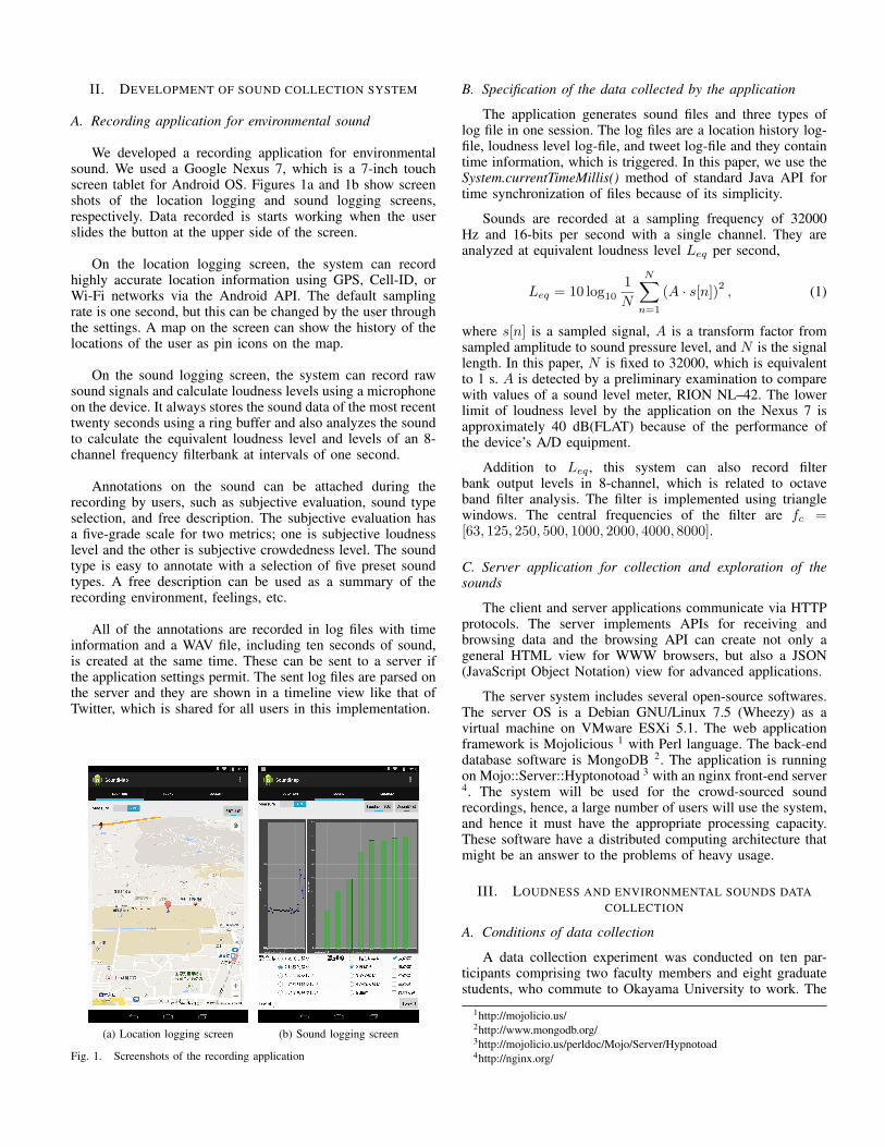
Figure 2a and 2b are the average loudness levels asfunctions of the subjective loudness level and subjective crowd-edness level, respectively. The average value is calculated asthe average of the data from the ten participants, and the errorbars are indicative of 90%-confidential intervals. We find twoclasses for subjective loudness to consider overlapping errorbars in Figure 2a, that is, L1, L2, and L3 are the “quiet”class, and L4 and L5 are the ”noisy” class. Figure 2b hasa similar tendency, that is, L1 is ”empty” and the others are”not empty.” The existence of two classes is not trivial becauseof the design of our questionnaires; however, its long errorbars display the importance of listener-specific information forsound interpretation.

TABLE I. TYPE OF ENVIRONMENTAL SOUND AND ITS DISTRIBUTION

Type of sound unlabeled (−1) labeled (+1)T1 Human speech 386 130T2 Sound of birds 447 69T3 Sound of insects 479 37T4 Sound of cars 318 198T5 Sound of wind 492 24

40

50

60

70

80

L1 L2 L3 L4 L5

Avera

ge o

f lo

udness level [d

B]

Subjective loudness

(a) Subjective loudness

40

50

60

70

80

C1 C2 C3 C4 C5

Avera

ge o

f lo

udness level [d

B]

Subjective crowdedness

(b) Subjective crowdedness

Fig. 2. Average Loudness as a function of a subjective evaluation. The errorbars indicates 90% confidence intervals as estimations of average loudnesslevels for the subjective level of each participant.

IV. VISUALIZATION SYSTEM FOR LOUDNESS ANDENVIRONMENTAL SOUNDS

The system statistically processes loudness data withspatio-temporal indexes; latitude, longitude, and time. Theamount of data, sum of data, and squared-sum of data ineach index is calculated as a sufficient statistic of Gaussiandistribution. These parameters are updated on demand byuploading data from users.

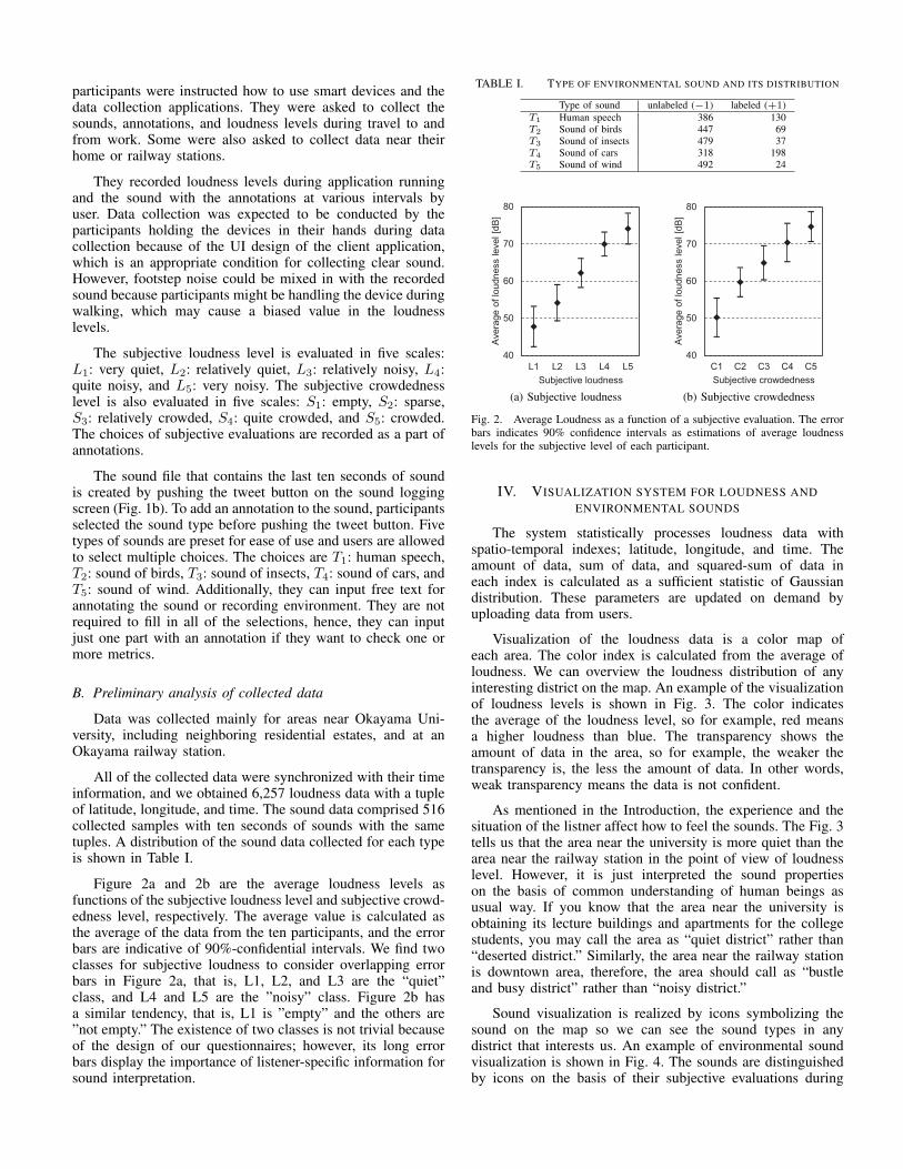
Visualization of the loudness data is a color map ofeach area. The color index is calculated from the average ofloudness. We can overview the loudness distribution of anyinteresting district on the map. An example of the visualizationof loudness levels is shown in Fig. 3. The color indicatesthe average of the loudness level, so for example, red meansa higher loudness than blue. The transparency shows theamount of data in the area, so for example, the weaker thetransparency is, the less the amount of data. In other words,weak transparency means the data is not confident.

As mentioned in the Introduction, the experience and thesituation of the listner affect how to feel the sounds. The Fig. 3tells us that the area near the university is more quiet than thearea near the railway station in the point of view of loudnesslevel. However, it is just interpreted the sound propertieson the basis of common understanding of human beings asusual way. If you know that the area near the university isobtaining its lecture buildings and apartments for the collegestudents, you may call the area as “quiet district” rather than“deserted district.” Similarly, the area near the railway stationis downtown area, therefore, the area should call as “bustleand busy district” rather than “noisy district.”

Sound visualization is realized by icons symbolizing thesound on the map so we can see the sound types in anydistrict that interests us. An example of environmental soundvisualization is shown in Fig. 4. The sounds are distinguishedby icons on the basis of their subjective evaluations during

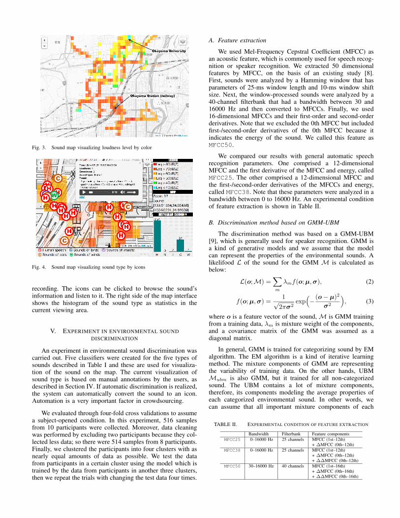
Fig. 3. Sound map visualizing loudness level by color

Fig. 4. Sound map visualizing sound type by icons

recording. The icons can be clicked to browse the sound’sinformation and listen to it. The right side of the map interfaceshows the histogram of the sound type as statistics in thecurrent viewing area.

V. EXPERIMENT IN ENVIRONMENTAL SOUNDDISCRIMINATION

An experiment in environmental sound discrimination wascarried out. Five classifiers were created for the five types ofsounds described in Table I and these are used for visualiza-tion of the sound on the map. The current visualization ofsound type is based on manual annotations by the users, asdescribed in Section IV. If automatic discrimination is realized,the system can automatically convert the sound to an icon.Automation is a very important factor in crowdsourcing.

We evaluated through four-fold cross validations to assumea subject-opened condition. In this experiment, 516 samplesfrom 10 participants were collected. Moreover, data cleaningwas performed by excluding two participants because they col-lected less data; so there were 514 samples from 8 participants.Finally, we clustered the participants into four clusters with asnearly equal amounts of data as possible. We test the datafrom participants in a certain cluster using the model which istrained by the data from participants in another three clusters,then we repeat the trials with changing the test data four times.

A. Feature extraction

We used Mel-Frequency Cepstral Coefficient (MFCC) asan acoustic feature, which is commonly used for speech recog-nition or speaker recognition. We extracted 50 dimensionalfeatures by MFCC, on the basis of an existing study [8].First, sounds were analyzed by a Hamming window that hasparameters of 25-ms window length and 10-ms window shiftsize. Next, the window-processed sounds were analyzed by a40-channel filterbank that had a bandwidth between 30 and16000 Hz and then converted to MFCCs. Finally, we used16-dimensional MFCCs and their first-order and second-orderderivatives. Note that we excluded the 0th MFCC but includedfirst-/second-order derivatives of the 0th MFCC because itindicates the energy of the sound. We called this feature asMFCC50.

We compared our results with general automatic speechrecognition parameters. One comprised a 12-dimensionalMFCC and the first derivative of the MFCC and energy, calledMFCC25. The other comprised a 12-dimensional MFCC andthe first-/second-order derivatives of the MFCCs and energy,called MFCC38. Note that these parameters were analyzed in abandwidth between 0 to 16000 Hz. An experimental conditionof feature extraction is shown in Table II.

B. Discrimination method based on GMM-UBM

The discrimination method was based on a GMM-UBM[9], which is generally used for speaker recognition. GMM isa kind of generative models and we assume that the modelcan represent the properties of the environmental sounds. Alikelifood L of the sound for the GMM M is calculated asbelow:

L(o;M) =∑m

λmf(o;µ,σ), (2)

f(o;µ,σ) =1√2πσ2

exp(− (o− µ)2

σ2

), (3)

where o is a feature vector of the sound, M is GMM trainingfrom a training data, λm is mixture weight of the components,and a covariance matrix of the GMM was assumed as adiagonal matrix.

In general, GMM is trained for categorizing sound by EMalgorithm. The EM algorithm is a kind of iterative learningmethod. The mixture components of GMM are representingthe variability of training data. On the other hands, UBMMubm is also GMM, but it trained for all non-categorizedsound. The UBM contains a lot of mixture components,therefore, its components modeling the average properties ofeach categorized environmental sound. In other words, wecan assume that all important mixture components of each

TABLE II. EXPERIMENTAL CONDITION OF FEATURE EXTRACTION

Bandwidth Filterbank Feature componentsMFCC25 0–16000 Hz 25 channels MFCC (1st–12th)

+ ∆MFCC (0th–12th)MFCC38 0–16000 Hz 25 channels MFCC (1st–12th)

+ ∆MFCC (0th–12th)+ ∆∆MFCC (0th–12th)

MFCC50 30–16000 Hz 40 channels MFCC (1st–16th)+ ∆MFCC (0th–16th)+ ∆∆MFCC (0th–16th)

class model are contained in the UBM. If we adapt or trainclass model using UBM as the seed model, we can obtainthe coordinated mixture components between class model andUBM model. It is an important property to introduce the Loglikelihood ratio (LLR).

First, the UBM model is trained for all data to constructthe classifier. Then, the UBM is used as a seed model in classmodels M1,M2,M3,M4, and M5, corresponding to classesT1, T2, · · · , T5, respectively. The class models are created onthe basis of MAP (Maximum a posteriori) adaptation method[10] for each class. We use a hyper-parameter τ = 10.

A retraining model is also created for comparison. Theretraining model is expected to achieve higher accuracy thanthe MAP adaptation model if the amount of training data issufficiently large.

The final decision is performed by thresholding a loglikelihood ratio (LLR) calculated by the UBM and each classmodel. This classifier can detect whether a certain class ofsound is included in the test sound (+1) or not (−1). TheLLR of class Tk for the test sound o is calculated from thelikelihood function L(o;M):

LLR(o, Tk) = logL (o;Mk)

L (o;Mubm). (4)

Then, the classifier Ck(·) of class k is constructed as thefollowing equation:

Ck(o) ={+1 if LLR(o, Tk) > 0,

−1 if LLR(o, Tk) ≤ 0.(5)

The mixture number of the GMM is updated by twice thenumber; i.e., training a 2-mixture model from the 1-mixturemodel, a 4-mixture model from the 2-mixture model, · · · , andfinally training a 256-mixture model from the 128-mixturemodel. EM training is repeated for a maximum of 20 timesfor each mixture number. The training and evaluation toolkitis HTK 3.4.1 [10].

C. Evaluation by F-measure

The F-measure is calculated from the following equation

F =2Ntp

2Ntp +Nfn +Nfp, (6)

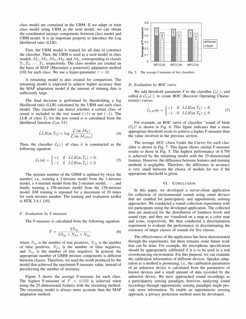
where Ntp is the number of true positives, Nfp is the numberof false positives, Nfn is the number of false negatives,and Ntn is the number of true negatives. In general, theappropriate number of GMM mixture components is differentbetween classes. Therefore, we used the result produced by themodel that achieved the maximum F-measure value, instead ofpreselecting the number of mixtures.

Figure 5 shows the average F-measure for each class.The highest F-measure of F = 0.522 is achieved whenusing the 25-dimensional features with the retraining method.The retraining model is always more accurate than the MAPadaptation method.

0.5

22

0.5

06

0.4

91

0.4

49

0.4

57

0.4

41

0

0.1

0.2

0.3

0.4

0.5

0.6

MFCC25 MFCC38 MFCC50

Avera

ge o

f F

-measu

re

Retrain

MAP

Fig. 5. The average F-measure of five classifiers

D. Evaluation by ROC curve

We add threshold parameter θ to the classifier Ck(·), andcalled it Ck,θ(·), to create ROC (Receiver Operating Charac-teristic) curves.

Ck,θ(o) ={+1 if LLR(o, Tk) > θ,

−1 if LLR(o, Tk) ≤ θ.(7)

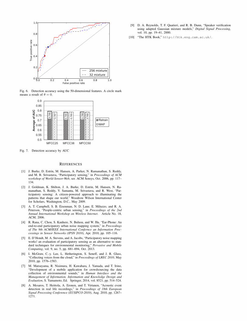
For example, an ROC curve of classifier ”sound of birds(T2)” is shown in Fig. 6. This figure indicates that a moreappropriate threshold exists to achieve a higher F-measure thanthe value involved in the previous section.

The average AUC (Area Under the Curve) for each clas-sifier is shown in Fig. 7. This figure shows similar F-measureresults to those in Fig. 5. The highest performance of 0.795is achieved by the retraining model with the 25-dimensionalfeatures. However, the difference between features and trainingmethods is negligible. Therefore, the difference in accuracyis very small between the choice of models for use if theappropriate threshold is given.

VI. CONCLUSION

In this paper, we developed a server-client applicationfor collection of environmental sounds using smart devicesthat are enabled for participatory and opportunistic sensingapproaches. We conducted a sound collection experiment withten participants using the developed application. The collecteddata are analyzed for the distribution of loudness levels andsound type, and they are visualized on a map as a color mapand icons, respectively. We then conducted a discriminationexperiment to evaluate the performance in discriminating theexistence of target classes of sounds for five classes.

The effectiveness of the application has been demonstratedthrough the experiments, but there remains some future workthat can be done. For example, the microphone specificationshould be appropriately calibrated if it is to be used in a realcrowdsourcing environment. For this purpose, we can examinethe calibration information of different devices. Speaker adap-tation as a method is promising, i.e., the calibration parametersof an unknown device is calculated from the parameters ofknown devices and a small amount of data recorded by theunknown device. We have approached sound recordings asa participatory sensing paradigm; however, analyzing soundrecordings through opportunistic sensing paradigm might pro-vide more information. To enable an opportunistic sensingapproach, a privacy protection method must be developed.

0.0 0.2 0.4 0.6 0.8 1.0False positive rate

0.0

0.2

0.4

0.6

0.8

1.0

True

pos

itive

rate

256 mixture32 mixture

Fig. 6. Detection accuracy using the 50-dimensional features. A circle markmeans a result of θ = 0.

0.7

95

0.7

85

0.7

88

0.7

87

0.7

85

0.7

85

0.5

0.55

0.6

0.65

0.7

0.75

0.8

0.85

0.9

MFCC25 MFCC38 MFCC50

Ave

rag

e o

f A

UC

Retrain

MAP

Fig. 7. Detection accuracy by AUC

REFERENCES

[1] J. Burke, D. Estrin, M. Hansen, A. Parker, N. Ramanathan, S. Reddy,and M. B. Srivastava, “Participatory sensing,” in Proceedings of ACMworkshop of World-Sensor-Web, ser. ACM Sensys, Oct. 2006, pp. 117–134.

[2] J. Goldman, K. Shilton, J. A. Burke, D. Estrin, M. Hansen, N. Ra-manathan, S. Reddy, V. Samanta, M. Srivastava, and R. West, “Par-ticipatory sensing: A citizen-powered approach to illuminating thepatterns that shape our world,” Woodrow Wilson International Centerfor Scholars, Washington, D.C., May 2009.

[3] A. T. Campbell, S. B. Eisenman, N. D. Lane, E. Miluzzo, and R. A.Peterson, “People-centric urban sensing,” in Proceedings of the 2ndAnnual International Workshop on Wireless Internet. Article No. 18,ACM, 2006.

[4] R. Rana, C. Chou, S. Kanhere, N. Bulusu, and W. Hu, “Ear-Phone: Anend-to-end participatory urban noise mapping system,” in Proceedingsof The 9th ACM/IEEE International Confernce an Information Proc-cessings in Sensor Networks (IPSN 2010), Apr. 2010, pp. 105–116.

[5] E. D’Hondt, M. A. Stevens, and A. Jacobs, “Participatory noise mappingworks! an evaluation of participatory sensing as an alternative to stan-dard techniques for environmental monitoring,” Pervasive and MobileComputing, vol. 9, no. 5, pp. 681–694, Oct. 2013.

[6] I. McGraw, C.-y. Lee, L. Hetherington, S. Seneff, and J. R. Glass,“Collecting voices from the cloud,” in Proceedings of LREC 2010, May2010, pp. 1576–1583.

[7] M. Matsuyama, R. Nisimura, H. Kawahara, J. Yamada, and T. Irino,“Development of a mobile application for crowdsourcing the datacollection of environmental sounds,” in Human Interface and theManagement of Information. Information and Knowledge Design andEvaluation, S. Yamamoto, Ed. Springer, 2014, vol. 8521, pp. 514–524.

[8] A. Mesaros, T. Heittola, A. Eronen, and T. Virtanen, “Acoustic eventdetection in real life recordings,” in Proceedings of 18th EuropeanSignal Processing Conference (EUSIPCO-2010), Aug. 2010, pp. 1267–1271.

[9] D. A. Reynolds, T. F. Quatieri, and R. B. Dunn, “Speaker verificationusing adapted Gaussian mixture models,” Digital Signal Processing,vol. 10, pp. 19–41, 2000.

[10] “The HTK Book,” http://htk.eng.cam.ac.uk/.