some topics in fluid mechanics - users home pages @ dma
TRANSCRIPT
Dottorato di Ricerca in MatematicaXI ciclo
Tesi per il conseguimento del titolo
some topics in fluid mechanics
Candidato : Luigi Carlo Berselli
Tutori : Prof. Hugo Beirao da Veiga Prof. Alberto Valli
Coordinatore : Prof. Sergio Spagnolo
Consorzio delle Universita degli Studi di Pisa, Bari, Lecce, Parma
Anno Accademico 1998/1999, discussa e approvata il 28/2/2000

c© Luigi Carlo Berselli
All rights reserved 2000
Abstract
Fluid-mechanics is an “ancient science” that is incredibly alive today. The modern technologiesrequire a deeper understanding of the behavior of real fluids; on the other hand new discoveriesoften pose new challenging mathematical problems.
In this framework a special role is played by incompressible viscous flows. The study of theseflows has been attached with a wide range of mathematical techniques and, today, this is a stimu-lating part of both pure an applied mathematics.
The aim of this thesis is to furnish some results in very different areas, that are linked by thecommon scope of giving new insight in the field of fluid mechanics. Since the arguments treatedare various, an extensive bibliography has been added. For the sake of completeness, there is anintroductory chapter and each subsequent new topic is illustrated with the will of a self-containedexposition.
The reader’s background is a good understanding of the classical arguments of functional anal-ysis and partial differential equations. In particular, it is needed a knowledge of the Sobolev spacesand of the variational formulation of linear elliptic and parabolic problems. The reader can find inthe book by Dautray and Lions (the second of the series cited in the bibliography) almost all therequired background material.
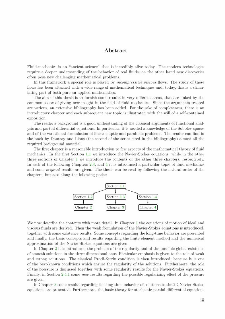
The first chapter is a reasonable introduction to few aspects of the mathematical theory of fluidmechanics. In the first Section 1.1 we introduce the Navier-Stokes equations, while in the otherthree sections of Chapter 1 we introduce the contents of the other three chapters, respectively.In each of the following Chapters 2,3, and 4 it is introduced a particular topic of fluid mechanicsand some original results are given. The thesis can be read by following the natural order of thechapters, but also along the following paths:
Section 1.1
Section 1.2 Section 1.3 Section 1.4
Chapter 2 Chapter 3 Chapter 4
We now describe the contents with more detail. In Chapter 1 the equations of motion of ideal andviscous fluids are derived. Then the weak formulation of the Navier-Stokes equations is introduced,together with some existence results. Some concepts regarding the long-time behavior are presentedand finally, the basic concepts and results regarding the finite element method and the numericalapproximation of the Navier-Stokes equations are given.
In Chapter 2 it is introduced the problem of the regularity and of the possible global existenceof smooth solutions in the three dimensional case. Particular emphasis is given to the role of weakand strong solutions. The classical Prodi-Serrin condition is then introduced, because it is oneof the best-known conditions which ensure the regularity of the solutions. Furthermore, the roleof the pressure is discussed together with some regularity results for the Navier-Stokes equations.Finally, in Section 2.4.1 some new results regarding the possible regularizing effect of the pressureare given.
In Chapter 3 some results regarding the long-time behavior of solutions to the 2D Navier-Stokesequations are presented. Furthermore, the basic theory for stochastic partial differential equations
iii
iv
is briefly recalled, together with the heuristic explanation of the role of random solutions in thetheory of Navier-Stokes equations. Finally, in Section 3.3.6 and 3.3.7 some new results regardingthe long-time behavior of the solution to the Stochastic Navier-Stokes equations are given.
In the last Chapter 4 a particular numerical strategy is proposed: the domain decompositionmethod. The techniques of domain decomposition are very interesting because they allow to split thecomputational effort into parallel steps and, consequently, they can use computational capabilitiesoffered by parallel computers. A rather detailed introduction of the known results for the Poissonequation is given in the Section 4.2. Then, motivated by the study of non-symmetric problems(as the ones arising in the discretization of the Navier-Stokes equations), in Section 4.3.2 and 4.4some new results regarding two classes of non-symmetric problems are presented. In particular,optimal convergence results for some iterative methods for the advection-diffusion equations aregiven. It is also proved a result concerning the time-harmonic Maxwell equations, which, thoughthey have a different structure, can be studied with a similar approach. We emphasize that ourinterest for the advection-diffusion equations is due to the fact that they are a model-problem fortransport equations and their solution gives also one of the main “computational kernels” of thecomputational fluid dynamics.
Acknowledgments
The author would like to thank Prof H. Beirao da Veiga for having introduced him to the study ofNavier-Stokes equations and for having stimulated him to interest to the different methods of pureand applied mathematics for fluid mechanics. It is a pleasure to thank Prof. F. Flandoli for havingintroduced the author to the fascinating field of stochastic partial differential equations, and forilluminating discussions regarding this subject. The author also thanks Prof. F. Saleri for havingperformed the numerical experiments and the University of Trento for the ospitality during thepreparation of this thesis. The author is grateful to Ph.D. E. Casella for her help in proof-reading,to Dr. G. Garberoglio for the Linux/GNU support and to Prof. L. Roi, for his help on everyproblem concerning typesetting with LATEX.
Contents
Abstract . . . . . . . . . . . . . . . . . . . . . . . . . . . . . . . . . . . . . . . . . . . . . iii
1 Navier-Stokes equations 11.1 Derivation of the equations . . . . . . . . . . . . . . . . . . . . . . . . . . . . . . . . 1
1.1.1 Euler equations . . . . . . . . . . . . . . . . . . . . . . . . . . . . . . . . . . . 11.1.2 Navier-Stokes equations . . . . . . . . . . . . . . . . . . . . . . . . . . . . . . 3
1.2 Main existence theorems . . . . . . . . . . . . . . . . . . . . . . . . . . . . . . . . . . 51.2.1 Function spaces and the Stokes operator . . . . . . . . . . . . . . . . . . . . . 51.2.2 Inequalities for the nonlinear term . . . . . . . . . . . . . . . . . . . . . . . . 81.2.3 Weak solutions . . . . . . . . . . . . . . . . . . . . . . . . . . . . . . . . . . . 91.2.4 Strong solutions . . . . . . . . . . . . . . . . . . . . . . . . . . . . . . . . . . 10
1.3 Long-time behavior . . . . . . . . . . . . . . . . . . . . . . . . . . . . . . . . . . . . . 121.3.1 Attractors . . . . . . . . . . . . . . . . . . . . . . . . . . . . . . . . . . . . . . 121.3.2 Determining modes, nodes and volumes . . . . . . . . . . . . . . . . . . . . . 141.3.3 Determining projections . . . . . . . . . . . . . . . . . . . . . . . . . . . . . . 16
1.4 A review of numerical methods in Fluid Dynamics . . . . . . . . . . . . . . . . . . . 171.4.1 Stokes equations . . . . . . . . . . . . . . . . . . . . . . . . . . . . . . . . . . 191.4.2 Navier-Stokes equations . . . . . . . . . . . . . . . . . . . . . . . . . . . . . . 201.4.3 Operator splitting: the Chorin-Temam method . . . . . . . . . . . . . . . . . 21
2 Regularity results 252.1 Regular solutions . . . . . . . . . . . . . . . . . . . . . . . . . . . . . . . . . . . . . . 25
2.1.1 On weak and strong solutions . . . . . . . . . . . . . . . . . . . . . . . . . . . 262.1.2 On the possible global existence of strong solutions . . . . . . . . . . . . . . . 292.1.3 The Prodi-Serrin condition . . . . . . . . . . . . . . . . . . . . . . . . . . . . 30
2.2 A short digression on the role of the pressure . . . . . . . . . . . . . . . . . . . . . . 332.2.1 Introduction of the pressure . . . . . . . . . . . . . . . . . . . . . . . . . . . . 34
2.3 On the possible regularizing effect of the pressure . . . . . . . . . . . . . . . . . . . . 352.3.1 Some results via the truncation method . . . . . . . . . . . . . . . . . . . . . 352.3.2 A result in the framework of Marcinkiewicz spaces . . . . . . . . . . . . . . . 37
2.4 Energy-type methods . . . . . . . . . . . . . . . . . . . . . . . . . . . . . . . . . . . . 392.4.1 Some regularity results . . . . . . . . . . . . . . . . . . . . . . . . . . . . . . . 40
3 On determining projections 473.1 A result on determining projections . . . . . . . . . . . . . . . . . . . . . . . . . . . . 47
3.1.1 Scott and Zhang interpolant . . . . . . . . . . . . . . . . . . . . . . . . . . . . 493.2 The Stochastic Navier-Stokes equations . . . . . . . . . . . . . . . . . . . . . . . . . 52
3.2.1 Weak solutions of the Stochastic Navier-Stokes equations . . . . . . . . . . . 54
vi CONTENTS
3.3 Determining projections for stochastic equations . . . . . . . . . . . . . . . . . . . . 573.3.1 The model problem: a reaction-diffusion equation . . . . . . . . . . . . . . . . 573.3.2 On determining projections for Stochastic Navier-Stokes equations . . . . . . 613.3.3 Stochastic framework . . . . . . . . . . . . . . . . . . . . . . . . . . . . . . . 613.3.4 The random attractor . . . . . . . . . . . . . . . . . . . . . . . . . . . . . . . 623.3.5 Energy-type estimate . . . . . . . . . . . . . . . . . . . . . . . . . . . . . . . 643.3.6 Determining projections forward in time . . . . . . . . . . . . . . . . . . . . . 653.3.7 Determining projections backward in time . . . . . . . . . . . . . . . . . . . . 67
4 Domain decomposition methods 694.1 Linear systems . . . . . . . . . . . . . . . . . . . . . . . . . . . . . . . . . . . . . . . 69
4.1.1 Iterative methods . . . . . . . . . . . . . . . . . . . . . . . . . . . . . . . . . . 704.1.2 Preconditioning . . . . . . . . . . . . . . . . . . . . . . . . . . . . . . . . . . . 71
4.2 Brief introduction to domain decomposition methods . . . . . . . . . . . . . . . . . . 724.2.1 A survey of Schwarz method . . . . . . . . . . . . . . . . . . . . . . . . . . . 724.2.2 Substructuring methods . . . . . . . . . . . . . . . . . . . . . . . . . . . . . . 754.2.3 Some iterative methods . . . . . . . . . . . . . . . . . . . . . . . . . . . . . . 79
4.3 Non-symmetric problems . . . . . . . . . . . . . . . . . . . . . . . . . . . . . . . . . . 864.3.1 Results for “slightly” non-symmetric problems . . . . . . . . . . . . . . . . . 884.3.2 Time-harmonic Maxwell equations . . . . . . . . . . . . . . . . . . . . . . . . 90
4.4 Advection diffusion equations and systems . . . . . . . . . . . . . . . . . . . . . . . . 1034.4.1 Adaptive methods . . . . . . . . . . . . . . . . . . . . . . . . . . . . . . . . . 1034.4.2 Coercive methods . . . . . . . . . . . . . . . . . . . . . . . . . . . . . . . . . 105
Bibliography . . . . . . . . . . . . . . . . . . . . . . . . . . . . . . . . . . . . . . . . . . 119Index . . . . . . . . . . . . . . . . . . . . . . . . . . . . . . . . . . . . . . . . . . . . . . . 127
Chapter 1
Navier-Stokes equations
The aim of this chapter is to present the Navier-Stokes equations, that are the equations governingthe motion of viscous fluids. We briefly derive the Navier-Stokes equations and then we recall someclassical results regarding different approaches to their study.
1.1 Derivation of the equations
In this section we follow essentially the book by Chorin and Marsden [CM93] and we explain themain features arising in the study of fluid-mechanics. We recall that the study of fluid-mechanicsis one of the most challenging fields for mathematicians and also for physicists. In the prefaceof the classical book by Landau and Lifshitz [LL59] fluid-mechanics is intended to be a branch oftheoretical physics, nevertheless difficult and still unsolved problems arise in the study of analytical,statistical and numerical properties of the solutions the equations of fluids.
1.1.1 Euler equations
We start with some basic facts of continuum mechanics. Let D ⊂ Rd be a region in the two (d = 2)or three (d = 3) dimensional space, filled with a fluid. Imagine a particle in the fluid and letu(x, t) = (u1, . . . , ud)(x, t) be a vector, depending on the space-time variable (x, t) = (x1, . . . , xd, t),denoting the velocity of a particle of fluid that is moving through x at time t. For each time t weassume that the fluid has a well-defined mass density ρ(x, t). Thus if W is any subregion of D, themass fluid in W at time t is given by m(W, t) :=
∫W ρ(x, t) dx, where dx is the volume element in
the plane or in the space. The assumption that ρ exists is a continuum assumption. The derivationof the equations is based on three basic physical principles: 1) mass is never created or destroyed;2) the rate of change of momentum of a portion of the fluid equals the force applied to it; 3) energyis neither created or destroyed.
Conservation of mass
As consequence of conservation of mass we have that
0 =d
dtm(W, t) =
∫W
∂ρ
∂tdx.
Let n denote the outward normal defined at points of ∂W and let dS denote the area (or (d − 1)-surface) element on ∂W. Since the volume flow rate across ∂W per unit area is u · n, the principle
2 Navier-Stokes equations
of conservation of mass can be stated as
d
dt
∫Wρ dx = −
∫∂W
ρu · n dS.
By using the divergence theorem the last equation becomes∫W
[∂ρ∂t
+ div (ρu)]dx = 0, where div u :=
∂u1∂x1
+ · · · +∂ud∂xd
.
Since the previous equality holds for all W it is equivalent to the following one
∂ρ
∂t+ div (ρu) = 0,
called the “continuity equation.”
Conservation of momentum
To define an ideal fluid we split the different forces acting on a piece of material into two classes:the stress forces (when a piece of material is acted on by forces across its surface, by the rest of thecontinuum) and the body forces (forces which exert a force per unit of volume as the gravity or anelectro-magnetic field).
Definition 1.1.1. We say that a continuum is an ideal fluid if for any motion of the fluid thereis a function p(x, t), called “pressure”, such that if S is a surface in the fluid, with a chosen unitnormal n, the force of stress exerted across the surface S per unit area, at x ∈ S and at time t, isp(x, t) n.
Many papers have been written on the hypotheses underlying this definition. We do not enterinto details, but we only remark that the absence of tangential forces implies that there is no wayfor rotation to start or to stop. In other words if curl u vanishes at time t = 0, it must be identicallyzero for every time. We recall that in three dimensions the vorticity field curl u is:
curl u(x, t) :=(∂u3∂x2
− ∂u2∂x3
,∂u1∂x3
− ∂u3∂x1
,∂u2∂x1
− ∂u1∂x2
)(x, t).
If W is a region in the fluid, at time t the total force exerted on the fluid inside W by the stressesis
S∂W =
force on W
= −∫∂W
pn dS.(1.1)
We now impose the conservation of momentum: let us write φ(x, t) (fluid flow map) for thetrajectory followed by the particle that is at point x at time t = 0. We assume φ to be smoothenough and we denote the map at fixed time t by φt(x, t) : x → φ(x, t). We denote by Wt themoving with the fluid region, where Wt := φt(W ). If it is given a body force per unit mass b(x, t),the balance of momentum reads as
d
dt
∫Wt
ρu dx = S∂Wt +∫Wt
ρb dx.
If J(x, t) denotes the Jacobian of φt, with straightforward calculations we get the following formula
∂
∂tφ(x, t) = J(x, t) div u(φ(x, t), t).(1.2)
1.1 Derivation of the equations 3
This formula is interesting because it shows that a fluid is incompressible (i.e. ,∫Wt
dx is constantin t) if and only if J ≡ 1 or if and only if div u = 0. By a change of variables and by using formula(1.2) we get (recall that D
Dt := ∂∂t + u · ∇)
d
dt
∫Wt
ρu dx =∫W
[D
Dt(ρu) + div u(ρu)
]φ J dx =
∫Wt
[D
Dt(ρu) + (ρdiv u) u
]dx.
and by using the conservation of mass we obtain
d
dt
∫Wt
ρu dx =∫Wt
ρDuDt
dx.
After reasoning on the integral formulation (since the last equation holds for each W ⊂ D) weestablish the differential form of the conservation of momentum1
ρDuDt
= −∇p + ρb.
Conservation of energy
We have developed d + 1 equations with the d + 2 unknowns ρ, p, and u. Consequently we needanother equation to avoid an over-determined problem. We suppose, as usual, that all the energy isthe kinetic (Ekin) one, and that the rate of change of the kinetic energy in a portion of fluid equalsthe rate at with the pressure and body forces work:
d
dtEkin(t) =
d
dt
12
∫Wt
ρ(x, t)|u(x, t)|2 dx = −∫∂Wt
pu · n dS +∫Wt
u · b dx.
The application of the divergence theorem and of the formulas obtained before shows that neces-sarily div u = 0. The Euler equations for a fluid filling D, derived firstly by Euler [Eul1755], arefinally
ρDuDt
= −∇p + ρb.
Dρ
Dt+ ρdiv u = 0.
div u = 0.
When the previous system is equipped with the tangential boundary condition u ·n = 0 on ∂D andinitial conditions on ρ and u, it is (in suitable spaces) a well-posed mathematical problem. For acollection of mathematical results regarding the Euler equations the reader can see the recent bookby P.-L. Lions [PLL96].
1.1.2 Navier-Stokes equations
The Euler equations describe an ideal fluid, but if we want to consider a more general fluid we needdifferent equations. The need of generalization comes from simple considerations about the kinetic
1The term DDt
is called the material derivative, because it takes into account the fact that the fluid is moving. If
we denote by a(t) the acceleration of a particle we have, by the chain rule, that a(t) := dudt = ∂u
∂t + u1∂u∂x1
+ · · ·+ud
∂u∂xd
= ∂u∂t + (u · ∇) u := Du
Dt .
4 Navier-Stokes equations
theory of matter. We do not enter into details, but we simply change our previous assumption2
(1.1) on the stress forces into the following one:force per unit of area
= −p(x, t) n + σ(x, t) n,
where σ is a matrix which depends only on the velocity gradient ∇u = ∂ui/∂xj . The matrix σmust be symmetric and for physical reasons regarding the invariance (with respect to orthogonaltransformations) of the equations we obtain
σ = λ(div u) I + 2µDS ,
where I is the identity matrix and DS is the symmetric part of ∇u. The last equation is generallywritten by putting all the trace terms in one term
σ = 2µ[DS − 1
3(div u)
]+ ζ(div u) I,
where µ is the first coefficient of viscosity and ζ = λ + 2µ/3 is the second coefficient.If we employ the transport theorem and the divergence theorem, as we did before, (we pass also
from the integral formulation to the differential one) we get the following equation:
ρDuDt
+ (u · ∇) u = −∇p + (λ + µ)∇(div u) + µ∆u,
where ∆u =∑d
i=1 ∂2u/∂x2i is the Laplacian of u. We observe that the Laplacian raises the order of
derivatives of u involved. This is accompanied by an increase in the number of boundary conditions:from the tangential condition we must pass to the no-slip condition u = 0. The physical need forthis boundary conditions comes from simple experiments involving flow past a solid wall. From themathematical point of view other conditions are suitable, but we shall confine to the no-slip one.
Remark 1.1.2. A crucial feature of the no-slip boundary condition is that it provides a mechanismby which a boundary can produce vorticity in the fluid.
We are interested to incompressible problems and we mainly deal with homogeneous3 (i.e. ,ρ = ρ0 = const.) viscous fluid. To study the scaling properties of the Navier-Stokes equations wemust write the equations in a non-dimensional form. We set ν = µ/ρ0 and p∗ = p/ρ0; for a givenproblem let L be a characteristic length and U a characteristic velocity. These numbers are chosenin a somewhat arbitrary way. If we measure x,u, and t as fraction of these scales we are changingthe variables and introducing the following dimensionless quantities
u∗ :=uU, x∗ :=
xL, t∗ :=
t
T.
By straightforward computations and by suppressing the stars (with an abuse of notation) weobtain the following equations
∂u∂t
+ (u · ∇) u + ∇p− 1R
∆u = 0,
2The fact that the force acting on S should be a linear function of n is not an assumption, but it derives frombalance of momentum. This result is known as Cauchy Theorem. Complete discussion with also historical remarksregarding the constitutive relation for σ can be found in Lamb [Lam93]. We recall that the Navier-Stokes equationswere introduced by Navier [Nav1822] and, while Stokes studied in [Sto1849] mainly the linearized problem, theequation inherited the names of both.
3We recall that the incompressibility conditions implies that, if the density ρ is constant in space, it is also constantin time because Dρ/Dt = 0.
1.2 Main existence theorems 5
where the dimensionless quantity R := LU/ν is the Reynolds number.With another abuse of notation (to have the equation as they are generally written in the mathe-matical literature) we write the equations with ν = 1/R. The complete set of incompressible andhomogeneous Navier-Stokes equations, driven by an external force f and with proper boundary andinitial condition, is finally
∂u∂t
+ (u · ∇) u− ν∆u + ∇p = f in D × [0, T ],(1.3)
div u = 0 in D × [0, T ],(1.4)u = 0 on ∂D × [0, T ],(1.5)u(x, 0) = u0(x) in D × 0,(1.6)
1.2 Main existence theorems
In this section we state some of the basic results regarding the mathematical approach to the Navier-Stokes equations. The main problem regarding the equations of incompressible fluid dynamics are:there exists a solution? Is it unique?
Many mathematicians have faced with this problem and the first satisfactory answer arrivedfrom Leray [Ler33, Ler34a, Ler34b]. He proved the basic existence and uniqueness results byusing the techniques of hydrodynamic potentials. These results were improved and the proof weresimplified by Hopf [Hop51], by using a more functional approach. The role of the weak solutionsbecame more and more important, especially after the appearance of the paper by Kiselev andLadyzenskaya [KL57] and the fundamental book by Ladyzhenskaya [Lad69]. We remark that inthe same years appeared the extremely complete4 paper by Berker [Berk63], in which big importanceis given to explicit (classical) solutions of the problem, in particular geometric situations.
In this section we outline some basic facts regarding the functional approach to the Navier-Stokesequations. We only state some basic results; for their proof we refer to the book by Constantin andFoias [CF88], if no other explicit reference is given.
1.2.1 Function spaces and the Stokes operator
In the sequel we shall use extensively the customary Sobolev spaces Wm,p(D) and Hk(D), respec-tively with norm ‖ . ‖m,p,D and ‖ . ‖k,D. For the reader not acquainted with these function spaces aclassical reference is Adams [Ada75]. Since we deal with evolution equations it is classical to usethe Banach spaces Lp(0, T ;B). They are the spaces of strongly (Lebesgue) measurable B-valuedfunctions v : [0, T ] → B such that∫ T
0‖v(t)‖pB dt < ∞ if 1 ≤ p < ∞ and ess sup
0<t<T‖v(t)‖B < ∞ if p = +∞.
These spaces are Banach spaces endowed with the norms:
‖v‖p,B =
[∫ T
0
‖v(t)‖pB dt
]1/p
if 1 ≤ p < ∞ and ‖v‖∞,B = ess sup0<t<T
‖v(t)‖B if p = +∞.
4The author would like to thank Prof. Cimatti for having pointed out this reference.
6 Navier-Stokes equations
Remark 1.2.1. We remark that for any p ∈ [1,+∞], Lp(0, T ;B) is the set of classes of functionsinduced by the equivalence relation
u ∼ v if and only if u = v a.e. in (0, T ),
and for simplicity we shall speak of functions instead of classes of functions.
In the treatment of the Navier-Stokes equations we shall use some appropriate Hilbert spaces.We define
V :=φ ∈ (C∞
0 (D))d : divφ = 0.
Let us denote by H and V the closure of V in (L2(D))d and (H10 (D))d, respectively. We equip H withthe (L2(D))d-norm denoted by | . |, induced by the usual scalar product (u,v) :=
∫D u·v dx. Since we
deal essentially with problems in bounded domains, we equip V with the norm ‖u‖2 :=∫D |∇u|2 dx.
The norm in V is equivalent to that one in (H10 (D))d (by the Poincare inequality) and it is inducedby the scalar product ((u,v)) =
∫D ∇u · ∇v dx.
We have the following proposition
Proposition 1.2.2 (Helmholtz decomposition). Let D be open, bounded, connected of class C2.Then (L2(D))d = H ⊕H1 ⊕H2, where H1,H2 are the following mutually orthogonal spaces,
H1 :=u ∈ (L2(D))d : u = ∇p, p ∈ H1(D), ∆p = 0
,
H2 :=u ∈ (L2(D))d : u = ∇p, p ∈ H10 (D)
.
The Stokes equations
The Stokes equations for (u, p) are−ν∆u + ∇p = f in D,div u = 0 in D,u = 0 on ∂D.
If (u, p) are smooth then, after multiplying by v ∈ V and by an integration by parts (recall that∇p belongs to a space orthogonal to H) we obtain ((u,v)) = (f,v).
Definition 1.2.3. We say that u is a weak solution of the Stokes equations if u ∈ V and
((u,v)) = (f,v) ∀v ∈ V.
We have the following proposition which states the role of the weak solutions.
Proposition 1.2.4. Let D be open bounded and of class C2. Then the following statements areequivalent
i) u is a weak solution of the Stokes equations;
ii) u ∈ (H10 (D))d and satisfies: there exist p ∈ L2(D) such that−ν∆u + ∇p = f in the sense of distributions,divu = 0 in the sense of distributions,u = 0 in the trace sense;
1.2 Main existence theorems 7
iii) u ∈ V achieves the minimum of J(v) := ν‖v‖2 − 2(f,v) on V.
By using the Lax-Milgram lemma in the separable Hilbert space V, we have the followingtheorem:
Theorem 1.2.5. Let D be open and bounded in some direction. Then (( . , . )) is a scalar productin V and for every f ∈ (L2(D))d there exists a unique weak solution of the Stokes equations.
We have also the following regularity result, for which we refer5 to Cattabriga [Cat61].
Theorem 1.2.6. Let D ⊂ Rd d = 2, 3 be bounded and of class Cr, r = max m + 2, 2, m ≥ −1.Let f belong to (Wm,α(D))d. Then there exists a unique u ∈ (Wm+2,α(D))d) and there exists aunique (up to an additive constant) p ∈ Wm+1,α(D) solutions of the Stokes equations. Moreover
‖u‖m+2,α,D + |‖p‖|m+1,α,D ≤ C‖f‖m,α,D,
where |‖ . ‖|m+1,α,D is the norm in Wm+1,α(D)/R.
The Stokes operator
We denote by P is the (Leray) orthogonal projection operator P : (L2(D))d → H. Let us assumethat D is bounded of class C2.
Definition 1.2.7. The Stokes operator A acting on D(A) ⊂ H into H is defined by
A : D(A) → H, A := −P∆.
We have the following proposition.
Proposition 1.2.8. The following results hold for the Stokes operator:
1) The Stokes operator is selfadjoint and D(A) = (H2(D))d ∩ V ;
2) The inverse of the Stokes operator, A−1, is a compact operator in H;
3) There exist wjj∈N, wj ∈ D(A) and 0 < λ1 ≤ · · · ≤ λj ≤ λj+1 ≤ . . . such that:
a) Awj = λjwj ,
b) limj→+∞ λj = +∞6,
c) wjj∈N is an orthonormal basis of H.
Remark 1.2.9. More regularity of ∂D is inherited by wj. In particular we have that if D is ofclass C l+2, l ≥ 0, then wj belongs also to (H l+2(D))d.
5See also, in the case α = 2, the simplified proof given in Beirao da Veiga [BdV97a], which avoids the methods ofpotential theory.
6We remark that the precise asymptotic behavior of the eigenvalues of the Stokes operator is known to be
limj→+∞
(|D|j
)2/d λj
(2π)2= ((n − 1)ωd)−2/d, where ωd = |B(0, 1)| denotes the Lebesgue measure of the unitary ball
and |D| that one of D, see Kozhevnikov [Koz84].
8 Navier-Stokes equations
Due to the previous result we can define, as usual, the fractional powers of A as follows:
Definition 1.2.10. Let α > 0 be real. For u ∈ D(Aα), where
D(Aα) :=u ∈ H : u =
+∞∑j=1
ujwj,
+∞∑j=1
λ2αj |uj |2 < +∞, uj ∈ Rd,
we define Aαu, by
Aαu :=+∞∑j=1
λαj ujwj for u :=+∞∑j=1
ujwj .
1.2.2 Inequalities for the nonlinear term
The presence of the nonlinear term is the most painful fact in the theory of Navier-Stokes equations.Its presence causes the lack of satisfactory existence and uniqueness theorems.
It is important to have good estimates on this term. In the Sobolev framework to treat thenonlinear term we introduce the following trilinear form
b(u,v,w) :=d∑
i,j=1
∫Duj
∂vi∂xj
wi dx =∫D
(u · ∇) v · w dx.(1.7)
We recall the following definition.
Definition 1.2.11. Let u,v ∈ (C(D))d. We define B(u,v) by
B(u,v) := P ((u · ∇) u),
where P is the Leray projector.
The trilinear term b(u,v,w) surely makes sense for u,v,w ∈ (C1(D))d, and the followingproposition states one important estimate.
Proposition 1.2.12. Let D be bounded, open and of class C l. Let s1, s2, s3 be real numbers suchthat 0 ≤ s1 ≤ l, 0 ≤ s2 ≤ l − 1 and 0 ≤ s3 ≤ l. Let us assume that
i) s1 + s2 + s3 ≤n
2if si =
d
2for i = 1, 2, 3
or
ii) s1 + s2 + s3 >n
2if si =
d
2for at least one i.
Then ∀u,v,w ∈ (C∞(D))d there exists a constant c, depending on s1, s2, s3, such that
|b(u,v,w)| ≤ C‖u‖1+[s1]−s1[s1],D
‖u‖s1−[s1][s1]+1,D‖v‖1+[s2]−s2
[s2]+1,D‖v‖s2−[s2][s2]+2,D
‖w‖1+[s3]−s3[s3],D
‖w‖s3−[s3][s3]+1,D.
The last proposition can be proven with a clever use of Holder and interpolation inequalities.We recall also the orthogonality property
b(u,v,v) = 0 ∀u ∈ V, ∀v ∈ (H10 (D))d,
which is of basic importance to get energy-type estimates.
1.2 Main existence theorems 9
1.2.3 Weak solutions
We now consider the Navier-Stokes equations in the particular cases of d = 2, 3, which are themost important from the physical point of view. The Navier-Stokes equations will be written inthe abstract form as functional equations in the Hilbert space H as follows:
dudt
+ ν Au + B(u,u) = f(1.8)
u(0) = u0.(1.9)
The solution will be a vector valued function u(t) such that Au(t) and B(u(t),u(t)) make sense.We now define the notion of weak solution and then we outline the proof of an existence theorem.
Definition 1.2.13. A weak solution of the Navier-Stokes equations (1.8) is a function u belongingto L2(0, T ;V ) ∩Cw(0, T ;H), satisfying du/dt ∈ L1loc(0, T ;V ′) and
<dudt
,v > +ν((u,v)) + b(u,u,v) = (f,v) a.e. in t ∀v ∈ V,(1.10)
u(0) = u0,(1.11)
where we denoted by V ′ the topological dual space of V, with pairing < . , . > . The space Cw(0, T ;H)is a subspace of L∞(0, T ;H) consisting of functions which are weakly continuous, i.e. (u(t),h) is acontinuous function for all h ∈ H. In particular the initial datum is taken in this sense.
The main result regarding weak solutions is the following, which is essentially due to Hopf [Hop51].
Theorem 1.2.14. There exists at least a weak solution of (1.8), for every u0 ∈ H and f ∈L2(0, T ;V ′). Moreover, the energy inequality
12|u(t)|2 + ν
∫ t
t0
‖u(s)‖2 ds ≤ 12|u(t0)|2 +
∫ t
t0
< f(s),u(s) >ds(1.12)
holds for all 0 ≤ t0 ≤ t ≤ T, a.e. t0 in [0, T ] and
if d=3 thendudt
∈ L4/3(0, T ;V ′)
if d=2 thendudt
∈ L2(0, T ;V ′).
We do not enter into details of the proof of Theorem 1.2.14, but we only outline that it is basedon three steps:
i) a Faedo-Galerkin approximation with smooth functions un : (0, T ) → Rk ⊂ V, for some
k ∈ N;
ii) the energy-type estimate
12d
dt|un|2 + ν‖un‖2 =< f,un >(1.13)
to get that un is bounded in L∞(0, T ;H) ∩ L2(0, T ;V ), uniformly in n;
iii) extraction of subsequences and additional compactness results (d = 3).
10 Navier-Stokes equations
1.2.4 Strong solutions
In this section we introduce the notion of strong solution and we show some results which highlightthe differences between problem in two and in three space dimensions.
Definition 1.2.15. A strong solution of the Navier-Stokes equations is a function u satisfying(1.10)-(1.11) and belonging to L∞
loc(0, T ;V ) ∩ L2loc(0, T ;D(A)) ∩ L2(0, T ;V ) ∩ L∞(0, T ;H).
The main tool to prove existence of strong solutions is an “high order” energy-type inequality.We consider again a Galerkin approximation, but this time we multiply the Navier-Stokes equationsby Aun and integrate over D. The “bad” term will obviously be b(un,un, Aun).
The two dimensional case
If d = 2, by setting s1 = 1/2, s2 = 1/2, and s3 = 0 in Proposition 1.2.12 we obtain
|b(un,un, Aun)| ≤ C|un|1/2‖un‖|Aun|.
By using Young inequality we have
|(f, Aun)| ≤ ν
4|Aun|2 +
‖f ‖2∞,H
ν.
These estimates lead to the inequality
d
dt‖un‖2 + ν|Au|2 ≤
2‖f ‖2∞,H
ν+
c
ν3|un|2‖un‖4(1.14)
By using the estimates on |un| and ‖un‖, which are known for weak solutions, and by applyingthe Gronwall lemma, we get the estimates needed to prove the following result, see Kiselev andLadyzenskaya [KL57].
Theorem 1.2.16. Let D ⊂ R2 be an open bounded set of class C2. Let u0 ∈ H, f ∈ L∞(0,∞;H).Then ∀T > 0 there exists a solution u of the Navier-Stokes equations satisfying
u ∈ L∞loc(0, T ;V ) ∩ L2loc(0, T ;D(A)) ∩ L∞(0, T ;H) ∩ L2(0, T ;V ).
The three dimensional case
In the three dimensional case we estimate again the nonlinear term by using Proposition 1.2.12with s1 = 1, s2 = 1/2, s3 = 0, but we can obtain the following estimate:
|b(un,un, Aun)| ≤ C‖un‖3/2|Aun|3/2.
Reasoning as before on the energy-type estimate, derived by multiplying the Navier-Stokes equa-tions by Aun, we get
d
dt‖un‖2 + ν|Au|2 ≤
2|f |2∞,H
ν+
c
ν3‖un‖6.(1.15)
By using the last estimate (1.15) it is possible to prove the following theorem
1.2 Main existence theorems 11
Theorem 1.2.17. Let D ⊂ R3 be an open bounded set of class C2. There exists a positive constantC such that for u0 ∈ V and f ∈ L2(0, T ;H) satisfying
‖u0‖2
ν2λ1/21
+2
ν3λ1/21
∫ T
0|f(s)|2 ds ≤ 1
4√C,(1.16)
there exists a solution u(t) of the Navier-Stokes equations belonging to L∞(0, T ;V )∩L2(0, T ;D(A)).
The condition (1.16) can be interpreted in various way: small initial data and external force,but arbitrary T. The same inequality shows also that if ‖u0‖ and ‖f ‖2,H are not small with respectto suitable expression in ν2 and λ1, only local existence can be inferred. We understand the needto deal with weak solutions, which are defined for any time interval [0, T ] even for d = 3. As weshall see with more detail later (see Chapter 2)
. . . even if u0 and f are very nice functions, in this case the existence of classical solu-tions of the Navier-Stokes equations is known, in general, only for short time intervals.
Remark 1.2.18. We remark that in the absence of boundaries the Leray projector P commuteswith the Laplace operator ∆. By absence of boundaries we mean either the case D = Rd or the caseD = Td, the dth dimensional torus. In the latter case we can speak of periodic boundary conditions.In this case the Navier-Stokes equations are studied as equations on the whole space Rd with thefollowing condition
u(x1 + 2π, x2, . . . , xd) = · · · = u(x1, . . . , xd−1, xd + 2π) = u(x1, . . . , xd) ∀ (x1, . . . , xd) ∈ Rd,
and there is no loss of generality to assume that∫D u0(x) dx = 0. We define Hper as the closure in
(L2(D))d of the set u ∈ (C1per(D))d : div u = 0 and
∫D
u(x) dx = 0,
where C1per(D) is the space of differentiable periodic functions. We also define Vper as the divergence-free subspace of (H1per(D))d, where Hm
per(D) are the periodic functions in Hm(D). By setting k =(k1, . . . , kd) ∈ Zd, we define, for m ≥ 0,
Hmper(D) :=
u : u =
∑k∈Zd
ckei(k1x1+···+kdxd),∑k∈Zd
(1 + |k|)2m|ck|2 < ∞ and c0 = 0,
with the norm‖u‖2m =
∑k∈Zd
(1 + |k|)2m|ck|2 < ∞.
We recall that since ck ∈ C we have to impose ck = c−k, to have real valued functions. We haveagain the Helmholtz decomposition (L2per(D))d = Hper ⊕ G, where G denotes a space of gradients,that is orthogonal to Hper.
With the periodic boundary conditions we have that if d = 2, then
b(um,um, Aum) ≡ 0.
The last equation shows one the main simplifications due to the use of periodic boundary conditions.
12 Navier-Stokes equations
1.3 Long-time behavior
In this section we briefly explain the basic results regarding the long-time behavior of the Navier-Stokes equations. When dealing with long-time analysis we restrict to the two dimensional case.In this case the solution globally exist and it is unique. Further results will be presented whennecessary. The main idea, underlying the results we shall show, is the following one: since theNavier-Stokes equations are dissipative, “probably” the dynamical system generated by their solution,can be described (asymptotically) with a finite number of degrees of freedom. The first results inthis direction are due to Foias and Prodi [FP67] and Ladyzenskaya [Lad72]. We shall present twoof the main approaches: attractors and determining projections.
1.3.1 Attractors
In this section we describe the main features of the attractors in metric spaces, see Babin andVishik [BV92]. We consider a dynamical system whose state is described by an element u(t)of a metric space H. The evolution of the system is described by the semigroup S(t). We recallthat a family of operators S(t)t≥0 that maps H into itself for each t, is called a semigroup ifS(t + s) = S(t) S(s), for s, t ≥ 0 and S(0)x = x, ∀x ∈ H. We assume at least that S(t) is acontinuous nonlinear operator for t ≥ 0. We give now the definition of ω-limit set.
Definition 1.3.1. We say that the orbit starting at u0 is the set⋃
t≥0 S(t)u0. For u0 ∈ H or forA ⊂ H we define the ω-limit set of u0 and of A respectively as
ω(u0) :=⋂s≥0
⋃t≥s
S(t)u0 and ω(A) :=⋂s≥0
⋃t≥s
S(t)A,
where the closures are taken in H.
Remark 1.3.2. We remark that φ ∈ ω(A) if and only if there exists a sequence φnn∈N ⊂ A anda real sequence tn → +∞ such that limtn→+∞ S(tn)φn = φ.
Another important definition is that one of functional invariant set.
Definition 1.3.3. A set X ⊂ H is a functional invariant set for the semigroup S(t) if
S(t)X = X ∀ t ≥ 0.
Trivial examples of a invariant set are
a) a singleton fixed point u0 or any union of fixed points;
b) any time-periodic orbit7, when it exists.
The discussion of other examples, less trivial than the ones above, can be found in Temam [Tem97],§1. In the same reference one can also find the proof of all results of this section. We start with anabstract lemma.
Lemma 1.3.4. Assume that for some nonempty subset A ⊂ H and for some t0 > 0 the set⋃t≥t0
S(t)A is relatively compact in H. Then ω(A) is nonempty, compact and invariant.
7An orbit is periodic if there exists 0 < T < +∞ such that S(T )u0 = u0.
1.3 Long-time behavior 13
Remark 1.3.5. The lemma above provides us examples of invariant sets whenever we can showthat ∪t≥t0S(t)A is relatively compact. This set can consist of a single stationary solution u∗, ifall the orbits starting form A converge to u∗ as t → +∞. It can also be a single periodic or aquasi-periodic8 solution or even a more complex object.
At this point it is clear that some compactness is needed. The problem reduces to show that theset
⋃t≥t0
S(t)A is bounded if H is finite dimensional; the same set should be bounded in somesubspace W, compactly embedded in H, if we deal with a problem in infinite dimensions.
Definition 1.3.6. An attractor is a set A ⊂ H that enjoys the following properties
i) A is a functional invariant set;
ii) A has an open neighborhood U such that, for every u0 in U S(t)u0 converges to A as t goesto +∞, i.e.
d(S(t)u0,A) → 0 as t → +∞,
where the distance is understood to be the distance of a point to a set
d(x,A) = infy∈A
d(x, y).
If A is an attractor, the largest open set U that satisfies ii) is called the basin of attraction ofA. We can express condition ii) by saying that A attracts the points of U . We shall say that Auniformly attracts a set B ⊂ U if
d(S(t)B,A) → 0 as t → +∞,
where d(B0,B1) is the semidistance9 of B0,B1, defined by d(B0,B1) = supx∈B0infy∈B1 d(x, y). We
can now define the key concept of global attractor.
Definition 1.3.7. We say that A ⊂ H is a global attractor for the semigroup S(t)t≥0 if A iscompact attractor that attracts the bounded sets of H. Its basin of attraction is then all of H.
It is easy to prove that such a set is necessarily unique and that such a set is maximal forinclusion relation among the bounded attractors and among the bounded functional invariant sets.For this reason it is also called the maximal attractor
Existence of attractors
To prove the existence of attractors we introduce the notion of absorbing sets and that one ofuniformly compact semigroup.
Definition 1.3.8. Let B be a subset of H and U an open set containing B. We say that B isabsorbing in U if the orbit of any bounded set of U enters into B after a certain time, dependingon the set:
∀B0 ⊂ U B0 bounded ∃ t∗(B0) such that S(t)B0 ⊂ B ∀ t ≥ t∗(B0).8An orbit is quasi-periodic if the function t → S(t)u0 is of the form g(ω1t, . . . , ωdt) where g is a periodic with
period 2π in each variable and the frequencies ωj are rationally independent.9We recall that the Hausdorff distance defined on the set of nonempty compacts subsets of a metric space is defined
by δ(B0,B1) := max(d(B0,B1), (B1,B0)). We remark that d is not a distance as d(B0,B1) = 0 implies only B0 ⊂ B1.
14 Navier-Stokes equations
Definition 1.3.9. Let S(t)t≥0 be a semigroup of operators from H into itself. We say thatS(t)t≥0 is a uniformly compact semigroup if for every bounded set B there exists t0, which maydepend on B, such that: ⋃
t≥t0
S(t)B is relatively compact in H.
The existence of a global attractor for a semigroup implies that of an absorbing set. Converselythe next theorem will show that a semigroup, which possesses an absorbing set and enjoys someother properties, has a global attractor.
Theorem 1.3.10. Let us suppose that H is a metric space and that the operators S(t) are con-tinuous and satisfy the semigroup property. Let us suppose furthermore that the operators S(t) areuniformly compact for t large.
If we also assume that there exists an open set U and a bounded B ⊂ U such that B is absorbingin U , then the ω-limit set of B is the global attractor in U . Furthermore if U is convex and connected,then A = ω(B) is connected too.
With this abstract result it is immediate to prove that the Lorenz system has the global attractor.The equations of this system are
x′ = −σ x + σ y,y′ = r x− y − x z,z′ = −b z + x y,
and this system is a three-mode Galerkin approximation (one in velocity and two in temperatureof the Boussinesq equation, for a fluid heated from below). The numbers σ, r, b represent non-dimensional quantities. This model was proposed by Lorenz [Lor63], as an indication of the limitsof predictability in weather prediction.
Attractors for the Navier-Stokes equations
We do not give the proof of the following result. The interested reader can find it in Temam [Tem97],§3–5. We only observe that it is based on application of the energy-type estimates (1.13)-(1.14).
Theorem 1.3.11. The dynamical system associated to the two-dimensional Navier-Stokes equa-tions possesses a global attractor. Furthermore the Hausdorff dimension of the global attractor Aturns out to be finite. (See also the note at the end of page 16)
In particular it is easy to check that the hypotheses of Theorem 1.3.10 are satisfied; moretechnical (not necessary in the sequel) tools are needs to show the finite dimensionality of theattractor.
1.3.2 Determining modes, nodes and volumes
The results of this section are mainly based on the results which followed the germinal paper byFoias and Prodi [FP67]. They proved that, at least asymptotically, the behavior of the solutionsto the Navier-Stokes equations can be described by the behavior of a finite dimensional system or,in other words, by a system of ordinary differential equations.
1.3 Long-time behavior 15
General setting
We consider the Navier-Stokes equations with two external forces f,g and we denote by u and vthe relative solutions. We assume that D is a bounded smooth susbset of R2 and that
limt→+∞
|(f − g)(t)| = 0.
We have various results on the behavior of u − v.
Determining modes
The basic result stated by Foias and Prodi [FP67] is the following one, which states that the behaviorof the solutions is described by that one of the projection on a finite number of eigenfunctions ofthe Stokes operator.
Theorem 1.3.12. Let D, f,g satisfy the hypotheses described above. Then there exists N, whichdepends only on ν,D, f,g, such that
limt→+∞
‖PN (u − v)(t)‖R2N = 0 implies limt→+∞
|(u − v)(t)| = 0,
where PN denotes the projection operator on the subspace spanned by the first N eigenfunctions ofthe Stokes operator
PN : V → VN := span < w1, . . . ,wN > .
This result is very important, but of no practical use, because the eigenfunctions of the Stokesoperator are no computable, unless we study problems with periodic boundary conditions.
Determining nodes
Another result in this direction was given by Foias and Temam [FT84]. They proved that if thelarge time behavior of the solutions is known on an appropriate discrete set (nodes), then the largetime behavior of the solution itself is totally determined.
It is given a set of points EN = x1, . . . ,xN ⊂ D, then the density of this set is measured inthe following way. We associate to every point x ∈ D its distance to EN by dN (x) := min
1≤j≤N|x− xj |
and we setdN := max
x∈DdN (x),
which will be the main parameter to measure density. We have the following theorem
Theorem 1.3.13. Let the same hypotheses on D, f,g of the previous Theorem 1.3.12 hold. If weassume that, as t → +∞,
u(xj , t) − v(xj, t) → 0 for j = 1, . . . , N,
then there exists a constant α = α(ν,D, f,g) such that if dN ≤ α, then
‖u(t) − v(t)‖ → 0 as t → +∞.
The interesting feature of this result is that the point xj can be, for example, the nodal pointsfor a finite element method or a collocation method. The result of Theorem 1.3.13 is then strictlylinked with the numerical analysis of Navier-Stokes equations. We observe that regular solutions,say at least belonging to (H2(D))d ⊂ (C(D))d a.e. in time, are needed to define the value at pointsin D.
16 Navier-Stokes equations
Determining finite element volumes
A further generalization is based on the idea that the behavior of non-smooth solution cannot becharacterized by nodal values, see Foias and Titi [FT91] and Jones and Titi [JT92]. We recall thatV ⊂ C(D), if d ≥ 2 and that if u is a weak solution, then u ∈ V a.e. t ∈ [0.T ]. A result, which doesnot use further regularity properties of the solutions, can be obtained by using the spatial mean ofthe solution.
We consider D := (0, L)2 and we study the problem with periodic boundary conditions. Wedivide D into N equal squares of side l = L/
√N, labelled by Qj . We define the average of solutions
on the square Qj by
〈u〉Qj =N
L2
∫Qj
u(x) dx, for 1 ≤ j ≤ N.
We have the following theorem.
Theorem 1.3.14. Let the same hypotheses on f,g of Theorem 1.3.12 hold. There exists a naturalnumber N = N(ν, f,g, L) such that if N ≥ N then
limt→+∞
〈u〉Qj − 〈v〉Qj = 0 for 1 ≤ j ≤ N implies limt→+∞
|u − v| = 0.
Precise estimates10 on the number of degrees of freedom are known and the fundamental pa-rameter is the Grashof number defined by
Gr :=1
λ1 ν2lim supt→+∞
|f(t)|.
We do not enter into details, referring to the paper by Jones and Titi [JT93].
1.3.3 Determining projections
The results on nodes, modes and volumes can be generalized with a more abstract setting, whichencompasses them. The definition of determining projection was given by Holst and Titi [HT97]
. . . an operator which projects weak solutions onto a finite-dimensional space is deter-mining if it annihilates the difference of two “nearby” weak solutions asymptotically,and if it satisfies a single approximation inequality.
We now give the precise results.
Definition 1.3.15. The projection operator RN : V → VN ⊂ (L2(D))d, N = dim(VN ) < +∞is called a determining projection operator for weak solutions of the d-dimensional Navier-Stokesequations if
limt→+∞
|RN (u(t) − v(t))| = 0,
implies thatlim
t→+∞|(u(t) − v(t))| = 0.
10Sharp estimates (periodic boundary conditions) for the number of determining modes, nodes and volumes is Gr.This bound must be compared to the bound Gr2/3(1 + logGr)1/3, which holds for the global attractor. We recallthat an estimate of order of Gr is in agreement with the heuristic estimates, which are based on physical arguments,that have been conjectured by Manley and Treve.
1.4 A review of numerical methods in Fluid Dynamics 17
The result that can be proven is the following one, see Holst and Titi [HT97].
Theorem 1.3.16. Let the same hypotheses on D, f,g of the previous Theorem 1.3.12 hold. Letthere exists a projection operator RN : V → VN ⊂ (L2(D))2, N = dim(VN ) < +∞ satisfying
limt→+∞
|RN (u(t) − v(t))| = 0(1.17)
and satisfying the following approximation inequality
∃ γ > 0 ‖u −RN (u)‖(L2(D))2 ≤ C1Nγ
‖u‖(H1(D))2 ∀u ∈ (H1(D))2.(1.18)
Then if N > C(λ1Gr)1/γ , where C is a constant independent of ν, f and g, the following estimateholds
limt→+∞
|u(t) − v(t)| = 0.
We do not give the proof of this result here, because we shall analyze the problem in Chapter 3.
Remark 1.3.17. We observe that:
a) the projection operator acts on weak solutions (say only in V );
b) the definition of determining projection encompasses each of the notions of determining modes,nodes, volumes;
c) an operator satisfying (1.17)-(1.18) can be explicitly constructed, as we shall show in the followingSection 3.1.1.
1.4 A review of numerical methods in Fluid Dynamics
In this section we review some basic techniques used in the numerical approximation of the Navier-Stokes equations. The basic framework will be that one of Finite Element Method. We only givethe definition and the reader can find the details in the classical book by Ciarlet [Cia78].
Given a coercive bilinear form a( . , . ) : X × X → R in the real Hilbert space X and givenf ∈ X, the Faedo-Galerkin method reads as
find xh ∈ Xh : a(xh, yh) = f(yh) ∀ yh ∈ Xh,
where Xh is a suitable finite dimensional subspace of X. The major result is the following
Proposition 1.4.1. Let a( . , . ) and f as before and let Xh be a family of finite dimensional sub-spaces of X. Assume that there exists a dense subset X ⊂ X such that
limh→+∞
infxh∈Xh
‖y − yh‖ = 0 ∀ y ∈ X .
Then, as h → 0, xh converges in X to the solution x of the “continuous problem”
find x ∈ X : a(x, y) = f(y) ∀ y ∈ X.
We recall that the Finite Element Method is a particular Faedo-Galerkin method in which, roughlyspeaking, the finite dimensional subspace, used to approximate the problem, is given and reallycomputable.
18 Navier-Stokes equations
The Finite Element Method
To introduce some concepts on finite element spaces we start from the following definition.
Definition 1.4.2. The triple (K,PK,NK) is called a finite element if
i) K ⊂ Rd is a domain with piecewise smooth boundary (the element domain);
ii) PK is a finite dimensional space of functions on K (the shape functions);
iii) NK = N1, . . . , Nk is a basis for P ′K (the nodal variables).
We define some other objects needed for the polynomial interpolation. We define P ds as the
space of polynomials in d variables of degree less or equal than s. We have that P ds is a linear
space, whose dimension is easily calculated to be(d+s
d
). As basic examples of finite element we
recall the triangular Lagrange element, i.e. , K is a triangle, PK = P 21 and NK = N1, N2, N3 withNi(v) = v(xi), where xi are the vertices of K. Another example is the Crouzeix-Raviart element inwhich the vertices are replaced by the midpoints of the edges. This examples can be generalized tohigh order polynomials and to higher dimensional simplices.
We now define the notion of local interpolant.
Definition 1.4.3. Given a finite element (K,PK,NK), let the set ϕidi=1 ⊆ PK be the basis dualto NK (i.e. 〈Nj , ϕj , 〉P ′
K,PK = δij). If v is a function for which all Ni ∈ NK are defined, then wedefine the local interpolant by
IKv :=d∑
i=1
Ni(v)ϕi.
Definition 1.4.4. A subdivision T of a domain D is a finite collection of d-simplices Ki suchthat:
i) Ki ∩ Kj = ∅ if i = j;
ii)⋃Ki = D;
iii) the faces (which are (d-1)-simplices) of each simplex Ki lie on ∂D or are faces of anothersimplex Kj .
In this way it is is possible to create finite dimensional subspaces of some function spaces definedon D, by piecing together finite elements (Ki,PKi ,NKi), with Ki belonging to a given subdivisionT .
We are now in position to define the notion of global interpolant.
Definition 1.4.5. Suppose D is a domain with a subdivision T . Assume each element domain Ki
in the subdivision is equipped with some type of shape functions PKi and nodal variables NKi suchthat (Ki,PKi ,NKi) form a finite element. Let f belong to a space on which the nodal variables arewell defined. The global interpolant is defined by
IT f |Ki = IKif, for all Ki ∈ T .
In our context we use as PKi polynomials of a given degree (equal for every Ki). It is easy tosee that if v belongs just to P, then its global interpolant is v itself.
Since without further assumptions on a subdivision no regularity properties can be asserted forthe global interpolant we must give some conditions on the subdivision.Let D ⊂ Rd be a connected, open bounded domain with Lipschitz polyhedral boundary.
1.4 A review of numerical methods in Fluid Dynamics 19
Definition 1.4.6. A simplicial subdivision T (i.e. a subdivision in which each Ki is a simplex) ofD is regular if
maxKi∈Th
hKi
ρKi
≤ γ0,
with the constant γ0 ≥ 1 independent of h. With ρK we denote the radius of the largest closed ballcontained in K and with hKi the diameter of Ki.
We define the mesh size h of a given subdivision T to be
h := supKi∈T
hKi
and we denote a subdivision T with mesh size h by Th.
The regularity condition means (roughly speaking) that the elements of Th do not shrink toomuch. The main result is the following one, see Ciarlet [Cia78].
Theorem 1.4.7. Let D be a polygonal domain of Rd, d = 2, 3, with Lipschitz boundary and let Thbe a regular family of subdivisions of D such that each Kj is affine equivalent to the unit d-simplex.If the bilinear form a( . , . ) is continuous and coercive on X = H10 (D) and
Xrh := xh ∈ C0(D) : xh|K ∈ P d
r ∀K ∈ Th,
then the finite element method converges. Moreover if the exact solution belongs to Hs(D) for somes ≥ 2, then the following error estimate holds
‖x− xh‖1,D ≤ Chl‖x‖l+1, with l = min (k, s − 1).
1.4.1 Stokes equations
When dealing with the numerical analysis of the Stokes problem it is simple to apply an abstractFaedo-Galerkin method in V. On the other hand it is very difficult to find really computable finitedimensional subspaces of V, i.e. , to find divergence-free polynomial spaces. To overcome thisproblem it is generally used the so-called mixed formulation in which the approximate solution uh
belongs to Vh ⊂ V which is a (not a-priori divergence-free) finite dimensional space of (H10 (D))d.The problem reads as: find uh ∈ Vh and ph ∈ Qh ⊂ L20(D) such that
ν((uh,vh)) + (div uh, ph) = (fh,vh) ∀vh ∈ Vh,(1.19)(div uh, qh) = 0 ∀ qh ∈ Qh,(1.20)
where L20(D) := Q = p ∈ L2(D) :∫D p dx = 0. We do not enter into details of the numerical
approximation of the Stokes operator, because we shall not use it. We only recall the basic factregarding the analysis of mixed problems, see Brezzi and Fortin [BF91].
Theorem 1.4.8. Let us assume that the spaces Vh and Qh satisfy the following compatibility con-dition (inf-sup or Ladyzenskaya-Babuska-Brezzi condition): ∃ βh > 0 such that
∀ qh ∈ Qh ∃ 0 = vh ∈ Vh :∫Dqh div vh dx ≥ βh
(‖vh‖0,D + ‖div vh‖0,D
)‖qh‖0,D.(1.21)
Then the problem (1.19)-(1.20) has a unique solution (uh, ph) ∈ Vh ×Qh.
20 Navier-Stokes equations
It is easy to show that if the inf-sup condition is not satisfied, then the problem is ill-posed andgreat effort has been done to find appropriate couples of spaces (Vh, Qh) satisfying (1.21). We donot give any detail regarding this topic, which is worth of a book itself, because we shall not usethe mixed formulation. For an accurate analysis regarding the mixed formulation and the Stokesproblem we refer, for example, to Brezzi and Fortin [BF91] and to Quarteroni and Valli [QV94],§7–9.
1.4.2 Navier-Stokes equations
In the study of time-dependent problems one possible approach is the semi-discretization, i.e. , theproblem is discretized only with respect to the space variables. This approach leads to the studyof systems of ordinary differential equations.
Semi-discrete approximation
In the numerical study of the Navier-Stokes equations we choose Vhh≥0, a family of finite dimen-sional subspaces of the divergence free subspace V ⊂ (H10 (D))d. With the semi-discrete approachwe reduce to the following problem: for each t ∈ (0, T ) find uh ∈ Vh such that
d
dt(uh,vh) + ν((uh,vh)) + b(uh,uh,vh) = (fh,vh) ∀vh ∈ Vh,
uh(0) = u0h,
where u0h is any approximation of u0 in Vh. For the same reason explained for the Stokes problemthe method described above is not suitable and a mixed formulation must be used. The mixedformulation reads as: for each t ∈ (0, T ) find uh ∈ Vh and qh ∈ Qh such that
d
dt(uh,vh) + ν((uh,vh)) + b(uh,uh,vh) + (div uh, ph) = (fh,vh) ∀vh ∈ Vh,
(div uh, qh) = 0 ∀ qh ∈ Qh,
uh(0) = u0h,
We note that the trilinear form b(u,u,v) has been replaced by the
b(u,v,w) :=12
[b(u,v,w) − b(u,w,v)] ,
for stability purposes. The analysis of this method has been done by Heywood and Rannacher [HR82]and the basic result is that if (Vh, Qh) satisfy the inf-sup condition (1.21), if
infv∈Vh
‖v − vh‖1,D + infqh∈Qh
‖q − qh‖0,D = O(h) ∀ (v, q) ∈ V ×Q,
if the initial datum is regular and if ∇u belongs to (L∞(0, T ;L2(D)))d×d, then
‖u − uh‖0,D ≤ KeK th2, ‖p− ph‖0,D ≤ K min t, 1−1/2eK th ∀ t ∈ (0, T ).
We remark that the results previously shown are suitable for moderately low Reynolds numbers.For high Reynolds number the convective term might induce numerical oscillations if not properlytreated. Stabilization can be introduced by using implicit finite difference methods or stabilizationterms. For the analysis of the numerical instability of advection-diffusion problems we refer toSection 4.4.2.
1.4 A review of numerical methods in Fluid Dynamics 21
1.4.3 Operator splitting: the Chorin-Temam method
The operator splitting (also known as fractional-step or splitting-up method) is a method of approx-imation of evolution equations based on a decomposition of the operators.
We have to approximate a linear evolution equationdudt
+ Au = 0, 0 < t < T
u(0) = u0,
where u belongs to a suitable Banach space X and A is a linear operator from X into itself. A firstway is to introduce, with a standard Finite Differences Method11, an implicit scheme and define asequence of vectors um, for m = 0, . . . , N, as follows: u0 = u0,
um+1 − um
k+ Aum+1 = 0, m = 0, . . . , N − 1.
We recall that N is an integer, T = kN, and k is the mesh-size.A second way is a splitting-up method, based on the existence of a decomposition of A as a sum
A =∑q
j=1Aj. Starting again with u0 = u0 we recursively define a family of elements um+j/q, forM = 0, . . . , N − 1, and j = 1, . . . , q as follows
um+j/q − um+(j−1)/q
k+ Ajum+j/q = 0, m = 0, . . . , N − 1, j = 1, . . . , q.
When um is known um+1 can be computed, in the case of an ordinary scheme, by the inversion ofthe operators I +k A. In the case of a fractional step method the computation of um+1 requires theinversion of the q operators I + k Aq and the algorithm is useful if all these operators are simplerto invert than I + k A.
The Chorin-Temam method
In the classical method introduced by Chorin [Cho67, Cho68] and Temam [Tem69], two12 operatorsA1 and A2 are considered. The operator A1 is defined by
A1u := −ν∆u + (u · ∇) u,
while the second one is an operator taking into account the term ∇p and the incompressibilitycondition div u = 0. This method is also called the Projection Method.
The interval [0, T ] is divided into N ∈ N intervals of length k and we set
f m :=1k
∫ mk
(m−1)kf(t) dt, for m = 1, . . . , N.
The projection method reads as follows: start with u0 = u0 and when um ∈ (L2(D))d, m ≥ 0, isknown, define um+1/2 ∈ (H10 (D))d by
1k
(um+1/2 − um,v) + ν((um+1/2,v)) + b(um+1/2,um+1/2,v) = (fm,v) ∀v ∈ (H10 (D))d,
11The derivative with respect to to time is approximated with an incremental ratio.12In this case we speak of a two-steps method.
22 Navier-Stokes equations
and then define um+1 ∈ H by
(um+1,v) = (um+1/2,v) ∀v ∈ H.
The method is called a projection method because in the first step it is solved a non linear ellipticproblem (without the incompressibility constraint); the second step amounts to project the solutiononto H. If we introduce the “approximate functions” u(j)k from [0, T ] with values in (L2(D))d
such that u(j)k := um+j/2 for mk ≤ t < (m + 1)k we have the following convergence result, seeTemam [Tem77] Ch. 3, §7.
Theorem 1.4.9. Let f ∈ L2(0, T ;H) and u0 ∈ H.If the dimension of the space is d = 2, then, as k → 0, the following convergence results hold:
u(j)k → u strongly in L2(D × (0, T )),
u(j)k∗ u weakly-star in L∞(0, T ; (L2(D))2),
u(j)k → u strongly in L∞(0, T ; (H10 (D))2),
where u is the unique solution of the Navier-Stokes equations.If the dimension of the space is d = 3, then there exists some sequence k′ → 0 such that:
u(j)k → u strongly in L2(D × [0, T ]),
u(j)k∗ u weakly-star in L∞([0, T ]; (L2(D))d),
u(j)k u weakly in L∞([0, T ]; (H10 (D))d),
where u is some solution of the Navier-Stokes equations.
We remark that the condition which defines um+1 can be written, with a strong formulation, asum+1 − um+1/2 + k∇pm+1 = 0 in D,div um+1 = 0 in D,um+1 · n = 0 on ∂D.
From this system it easily deduced that the approximate pressure pm+1 satisfies the homogeneousNeumann boundary value problem (A), which should be compared with the non-homogeneousNeumann boundary-value problem (E), satisfied by the exact pressure p.
(A)
−∆pm+1 =
1k
div um+1/2 in D,
∂pm+1
∂n= um+1 · n = 0 on ∂D,
(E)
∆p = div f −
d∑i,j=1
∂ui∂xj
∂uj∂xi
in D,
∂p
∂n= (f + ν∆u) · n = 0 on ∂D.
It is interesting to note that this discrepancy on the boundary conditions for the exact and theapproximate problem implies that pm converges only in a very weak sense to the exact pressure p;nevertheless, this does not affect the convergence of the scheme for the velocity field u, as we haveseen in the Theorem 1.4.9 above.
1.4 A review of numerical methods in Fluid Dynamics 23
The Chorin-Temam (or projection) method is very useful because the first step involves a prob-lem without the incompressibility constraint. In this way its discretization does not suffer of theproblems arising in the numerical study of the Stokes problem. A further step can be introducedto linearize the equations. For simplicity we restrict to a two-dimensional problem and we referto Temam [Tem77] Ch. III, §7 for more details. A three-steps method can be the following: startwith u0 = u0 and when um ∈ ((L2(D))2 is known, define um+1/3 ∈ (H10 (D))2 by:
1k
(um+1/3 − um,v) + ν((um+1/3,v)) + b1(um,um+1/3,v) = (f m,v) ∀v ∈ (H10 (D))2.
Then find um+2/3 ∈ (H10 (D))2 such that:
1k
(um+2/3 − um+1/3,v) + ν((um+2/3,v)) + b2(um+1/3,um+2/3,v) = (f m,v) ∀v ∈ (H10 (D))2,
and finally um+1 ∈ V is the solution to the following problem:
(um+1,w) = (um+2/3,w) ∀w ∈ V,
where we set
bi(u,v,w) :=12
∫D
2∑j=1
[ui∂vj∂xi
wj − ui∂wj
∂xivj
]dx for i = 1, 2.
Existence and uniqueness of the solutions of the first two steps follow in a standard manner fromcoercivity, by using the Lax-Milgram lemma. Furthermore, um+1 is simply a (L2(D))d orthogonalprojection.
This method has a natural finite dimensional counterpart in which the space (H10 (D))2 can bereplaced by the polynomial Finite Element Spaces (Xr
h)2, see Theorem 1.4.7. It is interesting tonote that the first two steps involve the discretization of standard elliptic problems, i.e. , problemswithout conditions on the divergence of the solution. The third and last step of a discrete problemis again a projection on a divergence-free subspace.
The convergence of the method at a finite dimensional level (and for different discretization ofthe space variable), is discussed in Temam [Tem77] Ch. 3, §7.
In the concrete applications it is very important to have efficient numerical methods to solvethe linear, non-symmetric and elliptic systems arising in the first two steps. Systems of this kindare known in literature as advection-diffusion systems. For these systems (but also the scalar non-symmetric problem presents the same pathologies) abstract results, as the Lax Milgram lemma,imply existence and uniqueness of the solution at both the infinite and finite dimensional level. Onthe other hand, their numerical approximation involves some difficult stability questions when theviscosity ν term is “small,” see Section 4.4.2.
Having in mind the Chorin Temam method the importance of the numerical analysis of advectiondiffusion equations becomes clear. These equations are not only a linearized model for the fluid-dynamic equations, but they are also a basic tool in some numerical methods for the Navier-Stokesequations. In Chapter 4 we shall discuss some numerical methods for solving non-symmetric ellipticequations and the numerical difficulties arising in their study.

24 Navier-Stokes equations
Chapter 2
Regularity results
In this chapter we recall some basic fact regarding uniqueness, and regularity for the solutions ofthe Navier-Stokes equations. We consider the problems regarding the possible global existence,in time, of smooth solutions in three dimensions. In particular we present the classical resultregarding strong solutions and the uniqueness conditions due to Prodi and Serrin, which ensuresalso the regularity of weak solutions. Then we explain the special role played by the pressure in thesystem of Navier-Stokes equations and we show how to reconstruct the pressure from the velocityfield. Some recent results concerning the regularity are presented. These results, due to Beiraoda Veiga, use the truncation method and give sufficient conditions for the regularity. They arebased on suitable combination of velocity and pressure. In the last section we reverse the standardapproach and we obtain new results regarding the smoothness of the velocity, by starting fromthe pressure. In particular the smoothness of the velocity field is proved by starting only fromsummability conditions on the pressure.
2.1 Regular solutions
In this section we briefly explain how is it possible to prove more regularity for the solutions of theNavier-Stokes equations. We recall that if f = 0, u0 ∈ V and the boundary of D ⊂ R3 is smooth,then there exists a fully classical solution (u, p) ∈ (C∞(D× (0, T )))4, on a time interval (0, T ) withT bounded below in terms of the Dirichlet norm ‖u0‖ of the initial datum. We present this result,that is due to Ladyzenskaya [Lad66]; a simple proof and additional remarks regarding this resultcan be found in Heywood [Hey80].
Without entering into details of sharp results, we show how the boot-strap argument works. Thisis one of the most powerful tools to prove regularity results. We restrict ourselves to the steady stateproblem, since it is rather standard to pass to the non-stationary problem, see Temam [Tem77],Ch. III, §3. Some difficulties arise if we want to have full regularity also at time t = 0, providedthe initial datum is smooth; for instance it is not sufficient that u0 ∈ (C∞(D))3∩V and that ∂D isof class C∞ to ensure that u ∈ (C∞(D × [0, T ]))3, for some T > 0. In this case some compatibilityconditions must be satisfied and these can be found in Temam [Tem82].
We remark that in the two dimensional case, the regularity results which hold for the stationarycase can be extended to the time-dependent Navier-Stokes equations. In three spatial dimensionsthe regularity results hold only locally in time.
The main idea is to consider the first term u of the convective term (u · ∇) u as a known term
26 Regularity results
and then to study the linear problem
−ν∆u + ∇p = −(v · ∇) u.
with v = u as regular as weak solutions are. To show how this method work we give some ofthe calculations needed to prove the regularity. Some distinction, between the problem in twodimension and that one in three dimensions, is needed.
The two dimensional case
The term (u · ∇) u equals∑d
i=1 ∂(uiu)/∂xi. If d = 2, we use the Sobolev embedding theorem toget that ui ∈ H10 (D) ⊂ Lα(D), for any 1 ≤ α < +∞. This implies that ∂(uiuj)/∂xi belongs toW−1,α(D). The regularity results for the Stokes operator show that ui belongs to W 1,α(D) and pbelongs to Lα(D). If now α > 2, we have that W 1,α(D) ⊂ L∞(D), hence ui ∂uj/∂xi belongs toLα(D). This implies that ui ∈ W 2,α(D) and p ∈ W 1,α(D). Repeating the same argument we findthat ui ∂uj/∂xi belongs to W 1,α(D) and consequently ui ∈ W 3,α(D) and p ∈ W 2,α(D). The sameargument can be used till the regularity of D and f allows to get regularity of the solutions of theStokes problem, see Theorem 1.2.6.
The three dimensional case
In the three dimensional problem we have to use different estimates. In particular we can onlyinfer that ui ∈ H10 (D) ⊂ L6(D). This implies that ui ∂uj/∂xi belongs to L3/2(D). By using againTheorem 1.2.6, we have that ui ∈ W 2,3/2(D) and this finally implies that ui ∈ Lα(D) for any1 ≤ α < ∞. Therefore,
∑di=1 ∂(uiuj)/∂xi ∈ W−1,α(D) for any 1 ≤ α < ∞ and we can use the same
proof given for d = 2.
2.1.1 On weak and strong solutions
In the previous Sections 1.2.3-1.2.4 we introduced the notion of weak and strong solution. Thestrong solutions are not classical solutions, but they are very important. We now give some addi-tional results which can be useful to understand the role of weak and strong solutions, in the theoryof Navier-Stokes equations. We recall the following result (a corollary of Proposition 1.2.12), whichis useful to estimate the trilinear term and that is stated as Lemma 1 in Ladyzenskaya book [Lad69].
Proposition 2.1.1. For any open set D ⊂ R2, we have that:
‖u‖L4(D) ≤ 21/4‖u‖1/2L2(D)
‖∇u‖1/2L2(D)
∀u ∈ H10 (D).
Proof. It suffices to prove the last inequality for v ∈ C∞0 (D). For such a v we write
|v(x)|2 = 2∫ x1
−∞v(ζ1, x2)
∂v(ζ1, x2)∂x1
dζ1
and therefore|v(x)|2 ≤ 2 v1(x2),
where
v1(x2) =∫ +∞
−∞|v(ζ1, x2)|
∣∣∣∣∂v(ζ1, x2)∂x1
∣∣∣∣ dζ1.
2.1 Regular solutions 27
By interchanging the role of x1 and x2 we have
|v(x)|2 ≤ 2 v2(x1) = 2∫ +∞
−∞|v(x1, ζ2)|
∣∣∣∣∂v(x1, ζ2)∂x2
∣∣∣∣ dζ2.We finally obtain∫
R2 |v(x)|4 ≤∫R2 v1(x2)v2(x1) dx ≤ 4
( ∫Rv1(x2) dx2
)( ∫Rv2(x1) dx1
)
≤ 4‖v‖2L2(R2)
∥∥∥∥ ∂v
∂x1
∥∥∥∥2L2(R2)
∥∥∥∥ ∂v
∂x2
∥∥∥∥2L2(R2)
≤ 2‖v‖2L2(D)‖∇v‖2L2(D).
This inequality is very simple, but it plays a very big role in the theory of Navier-Stokes equations.With Proposition 2.1.1 we can easily prove the following uniqueness result.
Theorem 2.1.2. Let D ⊂ R2 be open bounded and of class C2. Let f ∈ L2(0, T ;V ′). Two weak
solutions u1 and u2 of the Navier-Stokes equations must coincide, or in other words, weak solutionsare unique.
Proof. The proof of this theorem is very simple and makes use of the classical methods for linearequations, joint with a simple estimate for the nonlinear term. If u1 and u2 are two solutions, asusual, we define w := u1 − u2. It is easily seen that w solves the following problem:
dwdt
+ νAw + B(u1,w) + B(w,u2) = 0,
w(0) = 0.
We take the scalar product with w and we obtain the following equality
12d
dt|w|2 + ν‖w‖2 + b(w,u2,w) = 0.
We use the Holder inequality and Proposition 2.1.1 to deduce that |b(w,u2,w)| ≤ c|w|‖w‖‖u2‖.By applying the Young inequality (with exponents q = q′ = 2), we get
d
dt|w|2 ≤ c
ν‖u2‖2|w|2.
By using Gronwall lemma, we can infer the following inequality
|w(t)|2 ≤ |w(0)|2 e
c
ν
∫ t
0‖u2(s)‖2 ds.
Since w(0) = 0 and since u2 belongs to L2(0, T ;H), we can conclude that w(t) ≡ 0.
28 Regularity results
We try to use (at least formally, because du/dt is not regular) the same techniques for the threedimensional problems. If d = 3, by using the same argument of Proposition 2.1.1, we can prove thefollowing estimate:
‖u‖L4(D) ≤√
2‖u‖1/4L2(D)
‖∇u‖3/4L2(D)
∀u ∈ H10 (D).
If we mimic the proof of Theorem 2.1.2, we get into troubles. In fact we obtain that
d
dt|w(t)|2 ≤ c
ν4‖u2(t)‖4|w(t)|2
and we do not know wether∫ T0 ‖u2(t)‖4 dt is finite1 or not, and consequently we cannot use the
Gronwall lemma to conclude.This argument seems crude and one can think that sharper estimates can make the proof work.
We recall that each of the sophisticated methods used in the last seventy years to try to prove theuniqueness if d = 3, failed in a similar way.
The problem of uniqueness of weak solution is still open. In three dimensions we can prove thefollowing result, due to Kiselev and Ladyzenskaya [KL57].
Theorem 2.1.3. Let D ⊂ R3 be open bounded and of class C2 and let f belong to L2(0, T ;H).
Two solutions u1 and u2 of the Navier-Stokes equations belonging to L2(0, T ;D(A)) ∩ Cw(0, T ;V )must coincide.
Proof. We use the same techniques and the estimate |b(w,u2,w)| ≤ c|w|‖w‖‖u2‖1/2|Au|1/2, toobtain
d
dt|w|2 ≤ c
ν‖u2‖ |Au2| |w|2.
From the Gronwall lemma we have the following estimate
|w(t)|2 ≤ |w(0)|2 e
∫ t
0
c
ν‖u2(s)‖ |Au2(s)| ds
and, by using the hypothesis on u2, the integral is finite. Consequently we get that w ≡ 0.
Remark 2.1.4. With a completely different technique it is possible to prove the same result byassuming that only one of the two solutions is strong: in other words, strong solutions are uniquein the larger class of weak solutions.
A continuation principle
If we are concerned to the regularity of the weak solutions of the Navier-Stokes equations, wemay suppose D,u0 and f as smooth as we want (say again f = 0, to avoid inessential technicalarguments). We know that there exists a strong solution, at least in an time-interval [0, T0) and inparticular sup0≤t≤T0
‖u(t)‖ is finite.
1By the way we found that u2 ∈ L4(0, T ;V ) is a sufficient condition for uniqueness, and strong solutions satisfy it.It is possible to make this formal argument rigorous and, to have uniqueness, it is sufficient the weaker assumptionthat only one of the two weak solution belongs to L8(0, T ; (L4(D))3), see Serrin [Ser63].
2.1 Regular solutions 29
Let now T > T0; we know that there exists a weak solution u on (0, T ) and, from the previousremark, we know that u ≡ u on (0, T0). We consider the maximal interval of existence (0, T∗) (orlife-span) of strong solutions, where
T∗ := maxT > 0 : such that there exists a solution u ∈ L∞(0, T ;V ) ∩ L2(0, T ;D(A))
.
We have the following result
Proposition 2.1.5. Since strong solutions are unique, for a strong solution we have that neces-sarily
lim supt→T∗
‖u(t)‖ = ∞ if T∗ = ∞ and lim supt→T
‖u(t)‖ < ∞ if T < T∗ < ∞.
Proof. The proof follows by a contradiction argument. Suppose that [0, T∗) is the maximal existenceinterval of u. If lim supt→T∗ ‖u(t)‖ < ∞, then we could find c ∈ R and t as close as we want to T∗such that
‖u(t)‖ ≤ c.
From the global existence theorem we have a weak solution v(s) with v(0) = u(t0) ∈ V. The solutionv(s) would be also strong in a time interval (0, T1), depending on ‖v(0)‖ = ‖u(t0)‖ through relation(1.16). Since ‖u(t0)‖ is bounded from above as t tends to T∗, the corresponding T1 is boundedbelow (in other words T1 can be chosen uniformly for t0 near T∗.) If T∗−t0 < T1, we obtain a strongsolution u(s) := v(s+ t0) which coincides with u for t < T∗. Contradiction, because in this way weextended u(t) beyond T∗. The quantity ‖u( · )‖ becoming infinite is then a necessary condition forloss of regularity.
Remark 2.1.6. We finally understand the role of strong solutions. A strong solution is not aclassical solution at all, but it is unique in the class of weak solutions and furthermore a strongsolution is smooth as the initial datum u0, provided the boundary ∂D and f are smooth enough. Thelast sentence says that if we are in the life-span of a strong solution, the solution belongs at least toL∞(0, T ;V ) ∩ L2(0, T ;D(A)), but it is also more regular. In particular it has the same regularityof the data, till the norm in V is bounded, recall the result of Ladyzenskaya [Lad66] in Section 2.1.
2.1.2 On the possible global existence of strong solutions
We start by recalling that in Section 1.2.4 we showed that in dimension two strong solutions areunique and exist globally in time. In three dimensions the situation changes drastically: strongsolutions are unique, but they exist only for small initial data (or small times). In three dimensionswe can only prove that weak solution are global in time, but we do not have a uniqueness resultfor them.
One of the main open problems is to show that a solution which is smooth at one instant cannotdevelop a singularity at a later time. Many authors tried to find appropriate a-priori estimates forsmooth solutions, in order to use them in a continuation argument. All the efforts regarding thissubject failed because many conditions on the velocity were found, but we are not able to check ifthey are satisfied by weak solutions.
By following the exposition given by Heywood [Hey90], we suppose f ≡ 0 and the basic differ-ential inequality we have to deal with is the following one:
d
dt‖u(t)‖2 ≤ C
‖u(t)‖4 for d = 2,
‖u(t)‖6 for d = 3.
30 Regularity results
We essentially derived the last inequality in the previous chapter and in spite of its simplicity, it isthe basic point to understand the problems arising in the study of three dimensional Navier-Stokesequations.
We consider a solution with an hypothetical singularity2 at t = t∗, i.e. , a solution for which‖u(t)‖ → +∞ when t → t∗. We consider the function φ(t) which satisfies the following ordinarydifferential equation
d
dtφ(t) = C φ2(t) for d = 2,
d
dtφ(t) = C φ3(t) for d = 3.
These equations correspond to the differential inequalities for ‖u(t)‖2. Let φ1(t) ∈ C([0, T )) be thesolution corresponding to the initial datum φ1(0) = ‖u0‖2. Furthermore, let φ2(t) be a solutionchosen to have a singularity at t∗. The graph of φ2(t) lies below the graph of ‖u(t)‖2 and∫ t∗
t∗−Tφ2(s) ds ≤
∫ t∗
t∗−T‖u(s)‖2 ds.
Simple calculations show that∫ t∗
t∗−Tφ2(s) ds = ∞ if d = 2,
∫ t∗
t∗−Tφ2(s) ds =
√2
C
√T if d = 3.
By referring to the energy identity, which holds for smooth solutions,
12|u(t)|2 + ν
∫ t
0‖u(s)‖2 ds =
12|u(0)|2,
we see that a singularity is impossible if d = 2 and it is impossible in the three dimensional case if
12|u(0)|2 ≤
√2
C
√T .
In the last case the development of a singularity requires more than the available energy. Thissimple argument shows the critical point in the theory of Navier-Stokes equations.
2.1.3 The Prodi-Serrin condition
In the previous section we pointed out the importance of strong solutions. We observe that thetheory of Navier-Stokes equations is not satisfactory in the three dimensional case, because we haveexistence in a class (weak solutions) in which we do not have uniqueness and, on the other hand,we have uniqueness in a class (strong solutions) in which only local existence is known.
The problem was investigated in several directions and some sufficient conditions which ensurethe uniqueness of weak solutions were found. The best known condition is that one known asProdi-Serrin condition. The result, that we are going to show, was proved independently3 by
2This is the condition for the blow-up of a strong solution.3As it was pointed out to me by Prof. G.P. Galdi, the Prodi-Serrin condition (just for the pure Cauchy problem)
is also given in a footnote of the 1934 seminal paper by Leray [Ler34b]. The Prodi-Serrin condition should be called,more properly, Leray-Prodi-Serrin condition.
2.1 Regular solutions 31
Prodi [Pro59] and Serrin [Ser62]. The condition (2.1) seems very simple but, up to now, no resultensures that a weak solution satisfies it.
Theorem 2.1.7. Let d ≥ 3 and let u be a weak solution of the Navier-Stokes equations whichsatisfies the additional hypothesis
uj ∈ Lr(0, T ;Ls(D))d for2r
+d
s≤ 1, s ≥ d.(2.1)
Then such a solution is unique in the class
L2(0, T ;V ) ∩ L∞(0, T ;H) ∩ Lr(0, T ; (Ls(D))d)
Proof. We divide the proof into three steps.
Step 1) Estimate on the trilinear term.We consider the interesting limit case of (2.1): 2r + d
s = 1. By using the Holder inequality we get
|b(u,v,w)| ≤ C‖u‖(Ls(D))d‖v‖‖w‖(Lρ(D))d , if1s
+1ρ
=12.
For each u ∈ (C∞(D))d we have, by the Holder inequality,
‖u‖(Lρ(D))d ≤ ‖u‖2/r(L2(D))d
‖u‖d/s(L2d/(d−2)(D))
for1ρ
=2/r2
+d/s
2d/(d − 2).
By using the Sobolev embedding theorem, we have that H10 (D) ⊂ L2d/(d−2)(D) and consequently
‖u‖(Lρ(D))d ≤ C‖u‖2/r(L2(D))d
‖u‖d/s.
The last estimate shows that
|b(u,v,w)| ≤ C‖u‖(Ls(D))d‖v‖|w|2/r‖w‖d/s.(2.2)
Step 2) Regularity of the time-derivative.With the preliminary estimate (2.2) we can prove additional regularity of du/dt. We recall thata-priori du/dt ∈ L4/3(0, T ;V ′) while, if the Prodi-Serrin condition (2.1) is satisfied, we have thatdu/dt ∈ L2(0, T ;V ′).
By using the estimate (2.2) and by recalling that u ∈ L∞(0, T ;H) we have
|b(u,u,v)| = | − b(u,v,u)| ≤ C1‖v‖‖u‖(Ls(D))d |u|2/r‖u‖d/s,≤ C2‖v‖‖u‖(Ls(D))d‖u‖d/s.
By observing that t +→ ‖u(t)‖(Ls(D))d belongs to Lr(0, T ) and that t +→ ‖u(t)‖d/s belongs toL2s/d(0, T ), we get that
t +→ ‖u(t)‖(Ls(D))d‖u(t)‖d/s belongs to L2(0, T ).
Consequently (g,v) := b(u,u,v) with g belonging to L2(0, T ;V ′). This last result implies thatdu/dt ∈ L2(0, T ;V ′).Step 3) Proof of uniqueness.
32 Regularity results
Let u1 and u2 be two solutions. We define w := u1 − u2. By using the regularity on the timederivative we obtain
12d
dt|w(t)|2 + ν‖w(t)‖2 = −b(w(t),w(t),u2(t)).
An application of the method used in Step 1 (the following formula follows from (2.2) by inter-changing the role of u and w) gives
|b(w,w,u2)| ≤ C‖u2‖(Ls(D))d |w|2/r‖w‖1+d/s.
We define M(t) := ‖u2‖r(Ls(D))d and we use the Young inequality with exponents
p = r and p′ defined by1p′
= 1 − 1p
= 1 − 1r≤ by (2.1) ≤ 1 − 1
2
(1 − d
s
)=
s + d
2s.
We obtain|b(w(t),w(t),u2(t))| ≤ CM(t)1/r|w(t)|2/r‖w(t)‖1+d/s,
≤ ν‖w(t)‖2 + C3M(t)|w(t)|2,
and finally12d
dt|w(t)|2 ≤ C3M(t)|w(t)|2.
The last inequality and the fact that (by hypothesis) M(t) := ‖u‖r(Ls(D))d
belongs to L1(0, T ),proves that w(t) ≡ 0.
If d = 3 Theorem 2.1.7 can be compared with the results of uniqueness for strong solutions, that weknow to exist locally. In fact if u ∈ L∞(0, T ;V ) then u ∈ L∞(0, T ; (Ls(D))d) with 1/s = 1/2−1/d,and consequently
u ∈ Lr(0, T ; ((Ls(D))d),2r
+d
s= 1.
Remarks and references regarding the existence of solutions for d ≥ 4 can be found in J.-L. Li-ons [JLL69], Ch. 1.
Further regularity by the Prodi-Serrin condition
The Prodi-Serrin condition was introduced to study the uniqueness of the solutions, but it waslater discovered by Sohr [Soh83], that the condition
uj ∈ Lr(0, T ;Ls(D))d for2r
+d
s= 1 s ∈ (d,∞]
implies also regularity (provided the data are regular and the necessary compatibility conditionsare satisfied). We do not give the proof of this sharp result, but we only say that its proof is basedon fine estimates on the solution of linear Cauchy problems, see also Section 2.3.1.
2.2 A short digression on the role of the pressure 33
2.2 A short digression on the role of the pressure
When dealing with the Navier-Stokes equations we pointed out in Chapter 1 that the problem iswell-posed because we have d+ 1 equations and d + 1 unknowns. The equations satisfied by u is asemilinear parabolic system, but when we try to apply the standard variational techniques we comeinto some troubles. The main problem is that the pressure p does not satisfy a parabolic equation,but it is a Lagrange multiplier associated to the constraint div u = 0. If we apply the divergence tothe first (vectorial) equation we obtain the following:
−∆p =d∑
i,j=1
∂ui∂xj
∂uj∂xi
−d∑
i=1
∂fi∂xi
.(2.3)
This last equation is very useful in the study of Euler equations (ν = 0). In the case of inviscidfluids we have a well-posed elliptic problem if we couple (2.3) with the Neumann condition whicharise by taking the scalar product by n of the equation for the conservation of momentum.
When dealing with the Navier-Stokes equations, the boundary condition is
∂p
∂n= (f + ν∆u) · n on ∂D,
which is of no practical4 use (unless we restrict to D = Rd or to periodic boundary conditions),
because the elliptic problem for the pressure is not well posed. When dealing with D = R3, for
example, we can write the pressure as a function of u and f,
p(x, t) = G(u, f) := − 14π
∫R3
1|x− y|div
[(u · ∇) u + f
](y, t) dy
and we can study the equation
∂u∂t
+ (u · ∇) u − ν∆u + ∇G(u, f ) = f in R3 × [0, T ].
We observe that the operator G(u, f) is non-local, i.e. , the pressure has a non-local effect on thevelocity. In other words, the velocity field at each point y ∈ R3 is responsible for the values of thepressure gradient at a given point x ∈ R3; then the pressure gradients acts like a body force at thepoint x.
Remark 2.2.1. To see in more detail the role of the pressure, we consider a system of two coupledpartial differential equations in two scalar variables u, v
∂u
∂t= F1(Dαu,Dαv) |α| ≤ m,
∂v
∂t= F2(Dαu,Dαv) |α| ≤ m,
where α := (α1, . . . , αd) is a multi-index, Dα is the differential operator ∂|α|/∂xα11 . . . ∂xαdd and m
is a positive integer. When both u, v are known at time t, we can compute the right hand sidesand we can find the rates of change (partial derivative with respect to time) of u and v at the sametime. We can know the infinitesimal change of u and v at point x. The effect of u and v, each
4The compatibility condition∫D
∆p dx =∫∂D
∂p/∂ndS is not a-priori satisfied.
34 Regularity results
on the other, is local. The influence of the pressure is different. It is not the effect of a variablecoupled with the others, but it is a consequence of the incompressibility constraint divu = 0. A wayto impose local effect of the pressure is to come back to problems with variable density and to makethe constitutive assumption
p(x, t) = F(ρ(x, t)).
In this way the variables u and p are coupled in the ordinary (local) way. From the physical pointof view the incompressibility constraint implies the infinite propagation-speed of perturbations. Onthe other hand, in compressible models with variable density, the perturbations travel with a finitespeed. Unfortunately, the study of compressible models causes, up to now, mathematical difficultiesbigger than the ones arising in the study of incompressible equations.
2.2.1 Introduction of the pressure
The problems regarding the pressure were “solved” (or better hidden in the formulation) by usingthe Helmholtz decomposition, see Proposition 1.2.2. In this case the pressure disappears from theweak formulation, because gradients are orthogonal to divergence-free fields. The various theoremsof existence, that we have shown, do not involve the pressure. We introduce now the pressure inthe following way. Let us set:
U(t) :=∫ t
0u(s) ds, β(t) :=
∫ t
0B(u(s),u(s)) ds, F(t) :=
∫ t
0f(s) ds.
If u is a solution of the Navier-Stokes equations we have that U, β,F belong to C([0, T ];V ′). Byintegrating in time the abstract Navier-Stokes equations du/dt + ν Au + B(u,u) = f, we get
ν((U(t),v)) =< g(t),v > ∀v ∈ V, ∀ t ∈ [0, T ],
withg(t) := F(t) − β(t) − u(t) + u0, g ∈ C([0, T ];V ′).
We recall the following proposition, see Duvaut and J.-L. Lions [DL76] Ch. 3.
Proposition 2.2.2. Let D ⊂ Rd be an open set and let f = (f1, . . . , fd) such that fi are distribu-tions on D, for i = 1, . . . , d. Then we have the following result:
f = ∇p, p being a distribution, if and only if < f,v >= 0 ∀v ∈ V.
Let furthermore D ⊂ Rd be a bounded Lipschitz domain.
a) If a distribution p has all its first distributional derivatives in L2(D), then p itself belongs toL2(D) and
‖p‖L2(D)/R ≤ c1‖∇p‖L2(D), 0 < c1 ∈ R.
b) If a distribution p has all its first distributional derivatives in H−1(D), then p belongs to L2(D)
‖p‖L2(D)/R ≤ c2‖∇p‖−1,D, 0 < c2 ∈ R.
With the last proposition it is easy to conclude that for each t ∈ [0, T ] there exists q(t) ∈ L2(D),such that ∇q ∈ C([0, T ]; (H−1(D))3) which satisfies
−ν∆U(t) + ∇q(t) = g(t).
2.3 On the possible regularizing effect of the pressure 35
This result imply thatq ∈ C([0, T ];L2(D)).
By setting p = ∂q/∂t (the derivative is defined in the distributional sense) we obtain
∂u∂t
+ (u · ∇) u − ν∆u + ∇p = f.
In this way we can show a first regularity result for the pressure: it is the time derivative of acontinuous function with value in L2(D). We observe that the same argument shows that moreregularity on the velocity field implies more regularity on the pressure.
2.3 On the possible regularizing effect of the pressure
The problem of uniqueness of weak solutions or of their global regularity are basically open sinceappeared the papers by Leray cited in the bibliography. There were found many conditions of thefollowing kind: if the velocity satisfies condition . . . then it is regular. These results were foundwith the hope that, later, someone could be able to show that such a condition is satisfied by weaksolutions.
In this section we show some results which are guided by the same idea. A new approach is,instead of looking for conditions for the velocity, to look for conditions involving the pressure orsome combination of velocity and pressure.
We start by showing some recent results, which are obtained by using the classical truncationmethod. Then we show some results which are based on the use of Lα energy-type estimates.
2.3.1 Some results via the truncation method
The basic idea underlying the following results is to use (in a non standard way) some estimatesfor linear scalar parabolic equations. The idea used in the boot-strap argument is generalized anddifferent methods are applied.
We consider the following parabolic equation for the scalar unknown u :
∂u
∂t− ν∆u +
d∑j=1
bj∂u
∂xj=
d∑j=1
∂fj∂xj
− f in D × [0, T ] := DT ,(2.4)
and we treat in a classical way the linear initial-boundary value problem, which arise supplementingthe equation above with bounded initial and boundary data. An application of Theorem 7.1. Ch.III §7 of the classical book by Ladyzenskaja, Solonnikov and Ural’ceva [LSU67], gives the followingresult for (2.4).
Theorem 2.3.1. Assume that
bi, fi ∈ Lr(0, T ;Ls(D)) and f ∈ Lr/2(0, T ;Ls/2(D)),(2.5)
with
2r
+d
s< 1, r ∈ (2,∞], s ∈ (d,∞].(2.6)
(Note that the pairs (r, s) can be different for different coefficients, i.e., each coefficient bi, fi, fmay have its own couple (r, s), provided (2.5) and (2.6) are satisfied). Then the solution u of (2.4)belongs to L∞(DT ).
36 Regularity results
Moreover, if we restrict to the coefficients bi, we can replace (2.6) by the stronger condition
2r
+d
s= 1, s ∈ (d,∞](2.7)
If we consider the system of the Navier-Stokes equations, the results above do not apply. Oneidea to understand what results should be expected for the Navier-Stokes equations is to apply“formally” the same results where |u|2 plays the role of the fi, because (u · ∇) u = ∂(uiu)/∂xi.
In this case we should get that u is bounded if |u|2 ∈ Lr(0, T ;Ls(D)), with the condition r, sas in (2.6). For the Navier-Stokes equations the known result is that the solution is regular if usatisfy (2.7). This stronger result is also suggested by the use of the “linearized” equation
∂u∂t
− ν∆u + (v · ∇)u + ∇p = 0 in D × [0, T ],
where vi plays the role of the bi and u = v plays the role of the unknown. In this case the techniquesare similar to that one used in the boot-strap argument, see Sohr [Soh83].
Use of the pressure as a known term
Throughout this section | . | will denote indifferently the absolute value of a scalar, the modulus ofa vector or the Lebesgue measure of a set of Rd.
A completely new device, in the study of regularity, is to use the pressure p as a “known smoothterm.” We recall that equation (2.3) suggests some correspondence between p and |u|2. The scalarequation (p corresponds now to the fi’s) suggests that the solution of the Navier-Stokes equationsis regular if
p ∈ Lr(0, T ;Ls(D)) for2r
+d
s< 2, r ∈ (2,∞] and s ∈ (d,∞].
We recall that if we consider D = Rd or a problem with periodic boundary conditions, from (2.3)(and if f = 0) we can infer that ‖p‖L2(D) ≤ C‖|u|2‖L2(D). In these two cases the compatibilitycondition is satisfied (more precisely if D = Rd there are no conditions to be satisfied) and we canuse the classical regularity result for elliptic equations, see also Section 2.2. On the other side, itis an open question if ‖|u|2‖L2(D) ≤ C‖p‖L2(D). We remark that this condition is true for inviscidirrotational stationary flows via the Bernoulli law, but there is no heuristic reason to believe that asimilar relation holds for viscous fluids. The formal use of the results for linear parabolic equationssuggests that |p| - |u|2, at least as source of regularity. With this heuristic introduction we canshow the first result, which is due to Beirao da Veiga [BdV97b].
Theorem 2.3.2. Let u be a weak solution of the Navier-Stokes equations and let u0 be bounded.Assume that, for some positive real number k, the function φk, defined by
φk(x, t) =
|p(x, t)|
1 + |u(x, t)| if |u(x, t)| > k,
0 otherwise,
belongs to Lr(0, T ;Ls(D)), where (r, s) satisfy (2.6). Then u is bounded in DT .
As simple corollary, it is possible to prove the following result.
2.3 On the possible regularizing effect of the pressure 37
Corollary 2.3.3. If the following condition
|p|1 + |u| ∈ Lr(0, T ;Ls(D))(2.8)
holds, with (r, s) satisfying (2.6), then the solution u is bounded in DT .
This result gives a new insight into the possible regularity for the Navier-Stokes equations.Furthermore it involves (2.6) instead of condition (2.7), relative to the known results. The proof ofTheorem 2.3.2 is rather technical and since in the sequel we do not use its methods we only givean idea of the proof. By using the truncation method introduced by De Giorgi [DG57] we set, foreach k > 0
u(k) :=
(
1 − k
|u|
)u if |u| ≥ k,
0 otherwise.
By using u(k) as test function in the weak formulation of the Navier-Stokes equations, after somecalculations it is possible to arrive to the following inequality
12d
dt
∫D|u(k)|2 dx +
ν
2
∫D|∇u(k)|2 dx ≤ 2
νk2
∫Ak
|p|2|u|2 dx,
where Ak(t) := x ∈ D : |u(x, t)| > k. From this inequality it is standard to conclude byusing the following theorem, that can be found in the book by Ladyzenskaja, Solonnikov andUral’ceva [LSU67], Ch. II §1.
Theorem 2.3.4. Let u be a real function defined on DT such that∫DT
|u|2 + |∇xu|2 dx dt < +∞, and ess sup0<t<T
∫D|u|2 dx +
∫DT
|∇xu|2 dx dt < ∞.
Suppose that ess sup∂D×(0,T ) u ≤ h, for some h ≥ 0, and that for certain positive constants γ, κ thefollowing inequality holds:
|u(k)|DT≤ γ κµ
1+χr (k), k ≥ k.
Here µ(k) :=∫ T0 |Ak(t)|r/q, with 1/r + d/2q = d/4, ( with r > 2 if d > 2). Then ∃ β > 0 such that:
ess supDT
|u(x, t)| ≤ 2k[1 + 2
2χ+ 1
χ2 (β γ)1+1χ T
1+χr |D|
1+χq
].
2.3.2 A result in the framework of Marcinkiewicz spaces
In this section we show a regularity result, which holds in the Marcinkiewicz spaces. This result,which is strictly linked with that one of the previous section, is based on a different application of thetruncation method. The result we present in this section, is due again to Beirao da Veiga [BdV98].We start by defining the Marcinkiewicz spaces Lp
∗(E).
Definition 2.3.5. Let E be a measurable bounded subset of Rd and let 1 ≤ p < +∞. A measurablefunction f : E → R belongs to Lp
∗(E) if there exists a constant [f ]p such that
|y ∈ Rd : |f(y)| > σ| ≤(
[f ]pσ
)1/p∀σ > 0.(2.9)
The smallest constant [f ]p for which (2.9) holds is called the “norm” of f in Lp∗(E).
38 Regularity results
The most important property of these spaces is that they are “very close” to the classicalLebesgue spaces Lp(E). The following topological and algebraic inclusions hold:
Lp(E) ⊂ Lp∗(E) ⊂ Lp−ε(E), ∀ ε > 0.
We now investigate on regularity properties of solutions belonging to Lp(0, T ;Lp(D)) := Lp(DT )and Lp
∗(DT ) spaces. We recall that, up to the known results, a weak solution is regular if it satisfies
uj ∈ Ld+2(DT ), j = 1, . . . , d,
because the condition2r
+d
r= 1
implies r = d+ 2. Furthermore a similar result it is not known for any exponent less than d+ 2. Inthe framework of Marcinkiewicz spaces the following theorem can be proved.
Theorem 2.3.6. Let (u, p) be a weak solution of the Navier-Stokes equations. Assume that forsome θ ∈ [0, 1[ and some γ such that
2(d + 2)2θ + (1 − θ)(d + 2)
< γ < d + 2(2.10)
one hasp
(1 + |u|)θ ∈ Lγ∗(DT ).(2.11)
Then
ui ∈ Lµ(DT ), µ = (1 − θ)(d + 2)γd + 2 − γ
.(2.12)
Moreover if
p
1 + |u| ∈ Lγ∗(DT ), γ > d + 2,(2.13)
then u is bounded in DT .
We omit the proof of this result and we remark that it is obtained by using the truncationmethod with the following test functions:
u(k)(x, t) := max|u(x, t)| − k, 0.
The proof follows with the application of a technique, which generalizes that one introduced byStampacchia [Sta65]. We show the implications of Theorem 2.3.6, without other details about itsproof.
Remark 2.3.7. We start observing that if γ > (d+ 2)/(2− θ) then the solution is smooth, becausein this case µ > d + 2. If we consider the result and we suppose the “formal” relation |p| - |u|2,the assumption (2.11) corresponds to
uj ∈ L(2−θ)γ∗ (DT ).
From Theorem 2.3.6 we can infer that:
2.4 Energy-type methods 39
the known regularity on u increases if µ > (2 − θ)γ or equivalently (d + 2)/(2 − θ) < γ
the known regularity on u decreases if µ < (2 − θ)γ or equivalently γ < (d + 2)/(2 − θ)
the known regularity on u does not change if µ = (2 − θ)γ or equivalently γ = (d + 2)/(2 − θ)
and in the last case µ = (2 − θ)γ = d + 2 is the minimal exponent which gives regularity.
We start by observing that the case θ = 1 and γ > d + 2 falls within the range of applicability ofTheorem 2.4.4 with r = s = d + 2. It is interesting to consider the particular case with θ = 0. Inthis case we have hypotheses which involve only p and we can infer the following corollary.
Corollary 2.3.8. Let (u, p) be a weak solution of the Navier-Stokes equations. Assume moreoverthat
p ∈ Lγ∗(DT ), γ ∈ ]2, d + 2[.
Then
uj ∈ Lµ∗ (DT ), µ =
(d + 2)γd + 2 − γ
.
In particular if p ∈ Ld/2+1∗ (DT ), then uj ∈ Ld+2
∗ (DT ) and if p ∈ Lγ/2∗ (DT ), with γ > d + 2, then u
is “smooth”.
Remark 2.3.9. We remark that the last result gives the same regularity which can be obtained bysolving the heat equation
∂u
∂t− ν∆u = ∇p,
with a given p. This is interesting, because we obtain the same regularity which holds for the problemwith the nonlinear term dropped out. However the result is different because in the Navier-Stokesequations the pressure p is an unknown and not a given datum.
2.4 Energy-type methods
In this section we present other results regarding the effect of the pressure. The methods used arenow very similar to that one used in the construction of weak solutions. The energy inequality is nowreplaced by some Lα(D) estimates. This technique, which is the natural Lα(D), α = 2, counterpartof the energy method, was introduced by Beirao da Veiga [BdV87] to obtain the estimates neededto prove the existence of suitable solutions in Rd. This method consists in multiplying the Navier-Stokes equations by |u|α−2u, for suitable α > d, and then integrating by parts. In this way thepressure5 term does not disappear, but the problem is without boundaries and it is possible to use
5In this problem the pressure is determined by the condition p → 0 as |x| → +∞.
40 Regularity results
the Poisson equation (2.3) in the whole space Rd. With the classical Calderon-Zygmund inequality,we have, for some 0 < c ∈ R, the following estimate
‖p‖L(α+2)/2(Rd) ≤ c‖u‖2(Lα+2(Rd))d ,
which is strong enough to get (provided f and u0 are “smooth”) existence and uniqueness of weaksolutions such that
ui ∈ L2(0, T ;H1(Rd)) ∩ C([0, T ];Lα(Rd) ∩ L2(Rd)).
2.4.1 Some regularity results
We start this section by recalling the first (and unique, up to 1997) regularity result based on thepressure. We have the following theorem, which was proved by Kaniel [Kan68]. As in the previoussections D ⊂ Rd will be “smooth” and bounded.
Theorem 2.4.1. Let u be a weak solution of the three-dimensional Navier-Stokes equations, withsmooth initial conditions. If the associate pressure p satisfies
p ∈ L∞(0, T ;Lq(D)) for q >125,(2.14)
then u is smooth.
This theorem is based on the following technique: the Navier-Stokes equations are multipliedby the vector u3 := (u31, . . . , u
33); suitable calculations are performed to show that the V norm of
the solution is bounded on (0, T ) and consequently to infer that the solution is strong. Then thepassage to a smooth solution (if the data of the problem are smooth) is standard.
We now show some results which generalize that one of Theorem 2.4.1. The improvement isbased on sharper energy-type estimates, joint with classical regularity results.
Remark 2.4.2. To avoid non essential calculations we assume f = 0, but it is easy to see that thesame results holds if we add a forcing term belonging at least to L1(0, T ; (Lα(D))d).
To study the problem in the context of Lα(D) spaces, we need the space Hα, which is definedas the closure of V in (Lα(D))d. This space is the natural counterpart of the space H defined inSection 1.2.1. It is the space in which there were proved some existence and regularity results forproblem in bounded domains. These results are shown by using the different method of semigroupin Banach spaces, see Giga and Miyakawa [GM85] and Miyakawa [Miy81].
We start by recalling a simple lemma, that follows from Sobolev embedding theorem and thatwill be crucial in the sequel.
Lemma 2.4.3. Let |u|α/2 belong to H10 (D). Then
‖u‖αL
α dd−2 (D)
≤ C0
∫D|∇|u|α2 |2 dx,
with C0 a positive real constant.
Proof. We recall the following basic fact (see Adams [Ada75] for its proof):
H10 (D) ⊂ Lp∗(D) with1p∗
=12− 1
d.
2.4 Energy-type methods 41
This inclusion holds algebraically and topologically and we have
‖φ‖2Lp∗ (D) ≤ C0‖∇φ‖2(L2(D))d ∀φ ∈ H10 (D).(2.15)
This last inequality (2.15) applied to |u|α/2 gives the desired result.
The exponent (α d)/(d − 2) will play an important role in the sequel, similar to the exponent 6,which is the maximal one for the inclusion V ⊂ (Lp(D))3, in three dimensions. Recall for instancethe estimates for the nonlinear term we used in the previous sections.
We have the following results. The first one is due to Beirao da Veiga [BdV99] and it is in thesame spirit of the results of the previous section. The second one is due to Berselli [Ber99] and itis the claimed generalization of Kaniel Theorem 2.4.1.
Theorem 2.4.4. Let α > d. Assume that u0 ∈ Hα. Let (u, p) be a weak solution of the d-dimensional Navier-Stokes equations, such that
p
1 + |u| ∈ Lr(0, T ;Ls(D)),2r
+d
s< 1.
Then the solution is “smooth.”
Theorem 2.4.5. Let (u, p) be a weak solution of the d-dimensional Navier-Stokes equations withinitial conditions u0 ∈ Hα, for α > d. If the pressure p satisfies
p ∈ Lα(0, T ;Lα d
α+d−2 (D)),(2.16)
then the solution is “smooth.”
Remark 2.4.6. The condition u0 ∈ Hα is not restrictive and it is the natural one used to dealwith problem in the Banach spaces Lα(D) with α = 2, see Giga and Miyakawa [GM85].
Theorem 2.4.4 should be compared with Theorem 2.3.2 and Theorem 2.3.6 of the previoussection, since the results are very similar. From Theorem 2.4.5 we can immediately infer thefollowing corollary.
Corollary 2.4.7. Let d = 3, let p belong to Lα(0, T ;Lp(D)) with 9/4 < p < 3 and let u0 belong toHα, with α = p/(3 − p). Then the weak solutions of the 3-dimensional Navier-Stokes equations areregular. In particular this holds if p belongs to L∞(0, T ;Lp(D)).
Proof. If we restrict the results of Theorem 2.4.5 to the problem with d = 3, we have thatL
α dα+d−2 (D) = L
3α1+α (D) and
infα>3
3α1 + α
=94.
The lowest upper bound is attained for α = 3. We observe that
Lα(0, T ;L3α
1+α (D)) ⊃ L∞(0, T ;L3α
1+α (D)).
Moreover, for every 94 < p < 3, if we set α = p/(p − 3) > 3, we get
Lα(0, T ;L3α
1+α (D)) ⊃ L∞(0, T ;Lp(D)),
and this concludes the proof.
42 Regularity results
Remark 2.4.8. We remark that 9/4 (the best exponent) is strictly lower than 12/5 and in thisspecial setting we improve the cited result (2.14) by Kaniel. He assumed that u0 ∈ H10 (D) and thisalso implies that our summability condition on the initial datum u0 is satisfied, since p close to9/4 means that α is close to 3. Clearly, we also obtain a generalization of Kaniel result by takingα = 4. In this case the regularity holds if p belongs to L4(0, T ;L12/5(D)).
Remark 2.4.9. If we take our condition (2.16) and if we put r = α and s = α d/(d + α− 2), weget as a sufficient condition for regularity that
p ∈ Lr(0, T ;Ls(D)) with2r
+d
s= 1 +
d
α.(2.17)
Note that the right hand side is a real number greater than one and strictly lower than two. Itis worth noting that, at the light of the result shown before, (see Section 2.3.1) we expect that2/r+d/s < 2 (or even equal to 2) should be sufficient here. Note that the exponent two correspondsexactly to the sufficient condition (2.1), if p - |u|2. Also note that we arrive at this exponent if wecould take α = d. In fact in that case we will get a pressure belonging to Ld(0, T ;Ld2/2(d−1)(D)),for which condition (2.17) gives exactly two, the number relative to the hypothesis p - |u|2.
We start by observing that if a weak solution satisfies
u ∈ C(0, T ;Hα) and |u|α/2 ∈ L2(0, T ;H10 (D)),(2.18)
if u0 and f are regular and if the necessary compatibility conditions are satisfied, then it is “smooth,”see for example von Wahl [vW80]. Our aim will be to find some a-priori estimates to use theprevious remark.
The following lemma is the core of the proof of Theorem 2.4.4 and Theorem 2.4.5.
Lemma 2.4.10. Let (u, p) be a smooth solution of the Navier-Stokes equations in D×]0, T ]. Thenthe following estimate is satisfied
1α
d
dt‖u‖α(Lα(D))d +
ν
2Nα
α (u) + 4 να− 2α2
Mαα (u) ≤ (α− 2)2
2ν
∫Dp2|u|α−2 dx,(2.19)
where
Nα =[∫
D|∇u|2|u|α−2 dx
]1/αand Mα =
[∫D|∇|u|α2 |2 dx
]1/α.
Proof. We apply the “energy” method previously described, even if we study the problem in abounded domain D ⊂ Rd. The tool needed to prove (2.19) is simply to multiply the Navier-Stokesequations by |u|α−2u and to integrate over D. Then suitable integrations by parts are performedby taking into account that the fluid is incompressible (i.e. , div u = 0) and that the problem isequipped with no-slip (i.e. , u|∂D = 0) boundary conditions.
We observe that, since div u = 0, with an integration by parts we get:
b(u,u, |u|a−2u) = 0.
The term which requires more attention is
I := −∫D
∆uu|u|α−2 dx =∫D
d∑i,k=1
∂2ui∂x2k
ui
( d∑j=1
u2j
)(α−2)/2dx.
2.4 Energy-type methods 43
If we integrate by parts the boundary terms disappear and we obtain I = I1 + I2 with
I1 :=∫D
d∑i,k=1
∂ui∂xk
∂ui∂xk
( d∑j=1
u2j
)(α−2)/2dx,
and
I2 := (α− 2)∫D
d∑i,k=1
ui∂ui∂xk
uj∂uj∂xk
( d∑j=1
u2j
)(α−2)/2−1dx.
The term I1 is exactly Nαα (u). The term I2 requires some cares. Expanding |∇|u|α/2|2 we get
d∑i=1
( ∂
∂xi
( d∑k=1
u2k)α/4)2 =
(α4( d∑k=1
u2k)α/4−12uk ∂uk
∂xi
)2=
α2
4( d∑
k
u2k)(α−4)/2
u2k
(∂uk∂xi
)2,(2.20)
and finally we observe that
I2 = 4α− 2α2
∫D|∇|u|α/2|2 dx = 4
α − 2α2
Mαα (u).
First we obtain that1α
d
dt‖u‖α(Lα(D))d + νNα
α (u) + 4 να− 2α2
Mαα (u) = −
∫D∇p · u|u|α−2 dx.(2.21)
We remark that the terms Nα(u) and Mα(u) are the same which appear if D = Rn, since the
boundary terms vanish. We also recall the following inequality (which derives from (2.20)), thatwill be used in the calculations
|∇|u|α/2| ≤ α
2|u|α/2−1|∇u| a.e. in D.
If we integrate by parts the right hand side of (2.21) we have
−∫D∇p · u|u|α−2 dx = (α− 2)
d∑i,j=1
∫Dp∂ uj∂ xi
ui uj|u|α−2 dx,
=2(α− 2)
α
∫Dp|u|α/2−2
[d∑
i=1
ui
][d∑
i=1
∂
∂ xi|u|α/2
]dx,
and by observing that ∣∣∣∣∣∣∑i,j=1
uiuj∂uj∂xi
∣∣∣∣∣∣ ≤ |u|2|∇u| a.e. in D,
we obtain ∣∣∣∣∫D∇p · u|u|α−2 dx
∣∣∣∣ ≤ (α− 2)∫D|p||∇u||u|α−2 dx.
Finally, by using the Young inequality (q=q’=2) and Lemma 2.4.3, we arrive to the followinginequality ∣∣∣∣∫
D∇p · u|u|α−2 dx
∣∣∣∣ ≤ (α− 2)2
2 ν
∫Dp2|u|α−2 dx +
ν
2Nα
α (u),
which proves the lemma.
44 Regularity results
We now derive the two inequalities which prove the Theorems cited above. Given the a-priori esti-mates (2.22)-(2.24) both the proofs conclude by using the continuation argument and a regularityresult.
Proof of Theorem 2.4.4: a-priori estimate. Let now (r, s) satisfy 2/r + d/s < 1 and assume thats < ∞ ∫
Dp2|u|α−2 dx ≤
∫D
(p
1 + |u|
)2(1 + |u|)α s−d
d (1 + |u|)αds dx.
Since 2/s + (s− d)/s + (d− 2)/s = 1, we can use the Holder inequality to get∫Dp2|u|α−2 dx ≤ ‖p/(1 + |u|)‖2Ls(D)‖(1 + |u|)‖α(1− d
s )Lα(D) ‖(1 + |u|)‖
αds
Lαdd−2 (D)
.
By using the Young inequality with exponents r/2 and s/d we obtain, for ε > 0,∫Dp2|u|α−2 dx ≤ ε−
ss−d ‖p/(1 + |u|)‖rLs(D)‖(1 + |u|)‖αLα(D) + ε
sd ‖(1 + |u|)‖α
Lαdd−2 (D)
,
and we have
1α
d
dt‖u‖α(Lα(D))d +
ν
2Nα
α (u) + 4 να− 2α2
Mαα (u) ≤ ε−
ss−d
∥∥∥∥ p
1 + |u|
∥∥∥∥rLs(D)
2α−1(|D| + ‖u‖αLα(D)
)+
+εsd 2α−1
(α− 2)2
2ν
(|D|
d−2d + ‖u|‖α
Lαdd−2 (D)
).
Finally, by fixing ε and by using Lemma 2.4.3, we get6
1α
d
dt‖u‖α(Lα(D))d +
ν
2Nα
α (u) + 4 να− 2α2
Mαα (u) ≤ c1 + c2
∥∥∥∥ p
1 + |u|
∥∥∥∥rLs(D)
(|D| + ‖u‖(Lα(D))d
).
(2.22)
Proof of Theorem 2.4.5: a-priori estimate. We use the Holder inequality in the last term of (2.19)with exponents
p =α d
(α− 2)(d− 2)and q =
p− 1p
=α d
2(d + α− 2).
We observe that the condition p ≥ 1 is satisfied since α > d ≥ 3. We obtain∫Dp2|u|α−2 dx ≤ ‖u‖α−2
(Lp(α−2)(D))d‖p‖2L2q(D) ≤ ‖u‖α−2
(Lαdd−2 (D))d
‖p‖2L2q(D).(2.23)
Now we apply the Young inequality to (2.23) with exponents
p′ =α
α− 2and q′ =
α
2,
6With ε =
(ν2
2α−1(α− 2)
)d/s, c1 =
2ν(α− 2)
αC0|D|
d−2d , and c2 = 2α−2 (α− 2)2
ν
[2α−3α(α− 2)C0
ν2
] ds−d .
2.4 Energy-type methods 45
to get(α− 2)2
2ν
∫Dp2|u|α−2 dx ≤ 2ν
α− 2αC0
‖u‖α(L
α dd−2 (D))d
+ c1‖p‖αL
αdα+d−2 (D)
and the explicit value for c1 is c1 = (α−2)2ν α
[(α−2)2C0
4ν2
](α−2)/2.
By collecting the previous results (Lemma 2.4.3 and inequality (2.19)) we finally obtain
1α
d
dt‖u‖α(Lα(D))d +
ν
2Nα
α (u) + 2 να− 2α
Mαα (u) ≤ c1‖p‖α
Lα d
α+d−2 (D).(2.24)
We can now conclude the proof of Theorems 2.4.4-2.4.5 by using the comparison theorems forordinary differential equations. With inequality (2.22)-(2.24) and by using the hypotheses satisfiedrespectively by p/(1 + |u|) and p in a Gronwall inequality, we have that u ∈ L∞(0, T ;Hα) and that|∇u|α/2 belongs to L2(0, T ;H10 (D)).
We denote by t the lowest upper bound of the values in [0, T ] for which the velocity satisfiesthe condition (2.18):
u ∈ C(0, t;Hα) and |u|α/2 ∈ L2(0, t;H10 (D)).
We have that t > 0 and, as we claimed, the solution is regular in ]0, t[, see for example the classicalreferences by Giga and Miyakawa [GM85], Miyakawa [Miy81], Sohr [Soh83] and von Wahl [vW80].
Since estimate (2.22)-(2.24) holds in ]0, t[, it follows that u ∈ L∞(0, t;Hα) and, as consequenceof the hypothesis α > d, we have u ∈ C(0, t;Hα). By taking now u(t) as initial datum we canconstruct a solution in a larger interval and it is easy to see that necessarily t = T.
In the continuation argument we used the fact that if u is bounded with values in Hα, α > d thenu is also continuous with values in Hα. The proof of this result of strong continuity, which is basedon appropriate interpolation inequalities and a boot-strap argument, can be found in Beirao daVeiga [BdV99] and it is based on the argument developed for D = Rd in Beirao da Veiga [BdV87],Appendix B.

46 Regularity results
Chapter 3
On determining projections
In this chapter we analyze with more details the results regarding the long-time behavior of so-lutions. We start by presenting the results regarding the determining projections stated in Sec-tion 1.3.3. This result will be the starting point for some generalization. In particular we introduceseveral concepts regarding the analysis of stochastic partial differential equations and we studysome aspects concerning the long-time behavior of their solutions. The new result we prove arethe natural generalization to the stochastic framework of the result of Holst and Titi regarding theexistence of determining projections for the two dimensional Navier-Stokes equations.
3.1 A result on determining projections
We start this chapter by proving Theorem 1.3.16, that we claimed in Section 1.3.3. We give theproof by Holst and Titi [HT97] regarding the existence of a determining projection operator. Westart with a lemma, which is important in the analysis of the long time behavior of the Navier-Stokesequations. This lemma, whose proof can be found in Jones and Titi [JT93], is a generalization ofthe classical Gronwall lemma.
Lemma 3.1.1. Let T > 0 be fixed, and let α(t) and β(t) be locally integrable and real-valued on(0,+∞), satisfying
lim inft→∞
1T
∫ t+T
tα(τ) dτ =m > 0, lim sup
t→∞
1T
∫ t+T
tα−(τ) dτ = M < ∞,
limt→∞
1T
∫ t+T
tβ+(τ) dτ = 0,
(3.1)
where α− := maxα, 0 and β+ := maxβ, 0. Then if y(t) is an absolutely continuous, non-negativefunction on (0,∞) and if y(t) satisfies
y′(t) + α(t) y(t) ≤ β(t), a.e. on (0,∞),
then limt→∞ y(t) = 0.
Proof. From the standard Gronwall lemma, we obtain that
0 ≤ y(t) ≤ y(t0) e−∫ t
t0
α(σ) dσ+∫ t
t0
β+(τ) e−∫ t
τα(σ) dσ
dτ, for 0 < t ≤ t0.
48 On determining projections
From the assumptions on α, we may choose t0 large enough so that, for all s ≥ t0, we have∫ s+T
sα−(σ) dσ ≤ M + 1 and
∫ s+T
sα(σ) dσ ≥ m
2.
Hence, if t0 ≤ τ ≤ t and if k is an integer chosen such that τ + k T ≤ t ≤ τ + (k + 1)T, then
e−∫ t
τα(σ) dσ
= e−∫ τ+k T
τα(σ) dσ
e−∫ t
τ+k Tα(σ) dσ
≤ e−mk/2eM+1 ≤ M ′e−m/2T (t−τ),
for some M ′. By choosing an integer k0 such that t ≤ t0 + K0T ≤ t + T, we have that
∫ t
t0
β+(τ)M ′e−m (t−τ)/2T dτ ≤k0∑k=1
∫ t0+k T
t0+(k−1)Tβ+(τ)M ′e−m (k0T−kT−T )/2T dτ
≤(
supt≥t0
∫ t+T
tβ+(τ) dτ
)M ′ em/2
e − 1.
It follows that
lim supt→∞
|y(t)| ≤(
supt≥t0
∫ t+T
tβ+(τ) dτ
)M ′ em/2
e − 1
and by hypothesis (3.1) we can conclude that |y(t)| → 0 as t → ∞.
We can now easily prove that the long-time behavior of the solutions of the Navier-Stokes equationsis determined by their projection, if the projection operator satisfies:
‖u −RN (u)‖(L2(D))2 ≤ C1Nγ
‖u‖(H1(D))2 for 0 < C ∈ R.(3.2)
Proof of Theorem 1.3.16. Let u and v be solutions, corresponding to f and g respectively. We set,as usual, w := u − v. The application of the “energy method” and of the basic estimates for thenonlinear terms gives
12d
dt|w|2 + ν‖w‖2 ≤ ‖u‖|w|‖w‖ + ‖f − g‖V ′‖w‖.
An application of the Young inequality leads to
d
dt|w|2 + ν‖w‖2 − 2
ν‖u‖2|w|2 ≤ 2
ν‖f − g‖2V ′(3.3)
To bound the term on the left we use (3.2) in the following form
|w|2 ≤ 2N2γ
C‖w‖2 + 2‖RNw‖2(L2(D))2 ,
and we obtain
d
dt|w|2 +
(ν N2γ
2C− 2
ν‖u‖2
)|w|2 ≤ 2
ν‖f − g‖2V ′ +
ν N2γ
C‖RNw‖2(L2(D))2 .
3.1 A result on determining projections 49
The last inequality is of the form
d
dt|w(t)|2 + α(t)|w(t)|2 ≤ β(t).
To apply Lemma 3.1.1 to the last expression (and to prove that w → 0 as t → ∞) we need tocheck that the hypothesis (3.1) on α and β is satisfied. The conditions on α− and β+ are triviallysatisfied, because u,v and w belong to V. It remains to check that
lim inft→∞
1T
∫ t+T
tα(τ) dτ = m > 0,
and the last reduces to verify that, for some fixed T > 0, the following hold:
Nγ >2C2
νlim supt→∞
∫ t+T
t
2‖u(τ)‖2ν
dτ =4C2
ν2lim supt→∞
1T
∫ t+T
t‖u(τ)‖2 dτ.
Classical estimates on weak solutions yield
lim supt→∞
1T
∫ t+T
t‖u(τ)‖2 dτ ≤ 2
ν2lim supt→∞
‖f(t)‖2V ′ for T =C(D)ν
,
where C(D) is the best Poincare constant. Therefore if
N2γ ≥ 4C2
ν2
(2ν2
)lim supt→∞
‖f(t)‖2V ′ ,
thenlimt→∞
|w(t)| = 0.
Remark 3.1.2. From the proof it will follow that N should be of order of Gr2 (recall that Gr isthe Grashof number, defined at page 10) The bound can be improved to the claimed N - Gr if theno-slip conditions are replaced with the periodic boundary conditions, mainly for the simplificationdue to b(um,um, Aum) ≡ 0, see Remark 1.2.18. This identity show the lack of a boundary vorticityshedding source, when the boundary is absent, recall also Remark 1.1.2.
3.1.1 Scott and Zhang interpolant
The operator RN was introduced in the previous sections as an abstract operator. We now explainwhy it is needed and how to construct it explicitly.
We recall that the basic finite element interpolant (Lagrange and Crouzeix-Raviart and someothers) are defined for v at least in C0(K) and the nodal interpolant (i.e. , the nodal variables aredefined as evaluation at some points) are not well defined for functions in H1(D) with D ⊂ Rd, d ≥2. Since H10 (D) (or more precisely V) is the natural space in which we want to study the Navier-Stokes equations (it is the space in which weak solution live) it is necessary to introduce somedifferent interpolant. The Definition 1.4.2 in its generality encompasses also the setting needed todescribe the Scott and Zhang interpolant we are going to introduce. This interpolant, which wasintroduced by Scott and Zhang [SZ90, SZ92], will turn out to be well defined on H1(D) and alsoto have optimal properties of approximation.
The interpolant we shall construct needs an additional hypothesis on the subdivision: the quasiuniformity.
50 On determining projections
Definition 3.1.3. A simplicial subdivision Th is said to be quasi-uniform if there exists η > 0 suchthat
minKi∈Th
(ρKi) ≥ η h
we recall (see Section 1.4) that ρKi is the radius of the largest ball contained in Ki.
This condition means, roughly speaking, that all the simplices Ki are of comparable size andit is needed to make good estimates, since all the calculations can be done on a single referenceelement (the one for which K is the standard d-simplex). Observe also that if a family is quasi-uniform then it is regular, but not conversely. We point out that to construct the Scott and Zhanginterpolant the mesh needs to be regular. Furthermore, to make the approximation property (3.2)hold, the mesh needs also to be quasi-uniform.
We consider a finite element space Vh consisting of continuous piecewise polynomials:
Vh :=v ∈ C(D) : v|Ki
∈ PKi = P ds , ∀Ki ∈ Th
,(3.4)
and its subspace V0h, consisting of functions vanishing on the boundary.Now we present the Scott and Zhang interpolant, which defines an interpolation operator from
W k,p(D) into Vh, with
k ≥ 1 if p = 1 and k > 1/p otherwise.(3.5)
We construct the global interpolant Ih as follows: we shall use the same nodes xiNi=1 of theLagrange element and the nodal basis ϕiNi=1 of Vh to define the interpolation operator. We choosefor every node xi either a d-simplex (a triangle in our two dimensional problem) or a (d−1)-simplex(a side), according to the following rules
• if xi is an interior point of some d-simplex Ki ∈ Th we let
σi = Ki,
• if xi is an interior point of some face (which is a (d − 1)-simplex) K′ of a d-simplex Ki ∈ Thwe let
σi = K′,
• if xi is on a (d − 2)-simplex there are some degrees of freedom in the choice that producedifferent interpolant; we have in fact to pick one (d− 1)-simplex K′ in such a way that
σi ∈ K′ with the restriction K′ ⊂ ∂D if xi ∈ ∂D,
and we setσi = K′.
The condition K′ ⊂ ∂D is made for the purpose to preserve homogeneous boundary conditions ina natural way. It is the main improvement with respect to the Clement interpolant [Cle75], sincethe Scott and Zhang interpolant allows us to treat non-homogeneous problems, as for exampleelliptic problems with non zero Dirichlet data or Navier-Stokes equations with periodic boundaryconditions.
For each (d− 1)-simplex K′ of K there is a natural restriction of (K,P,N ) that defines a finiteelement
(K′,PK′ ,NK′) = (K,PK,NK)|K′ .
3.1 A result on determining projections 51
With NK′ we denote the evaluation points of NK that lie on the simplex K′ and PK′ = P d−1s . Let us
denote by n1 the dimension of P ds and by n0(σi) the dimension of P dimσi
s (that is(s+d
d
)or
(s+d−1d−1
)).
Let xi,1 = xi and let xi,jn0j=1 be the set of nodal points in σi, in which σi is the simplex associated
to xi.
We associate to the nodal basis ϕi,jn0j=1, defined on σi, the L2(σi)-dual basis ψi,jn0
j=1 (whichexists by the Riesz representation theorem):∫
σi
ψi,j(x)ϕi,k(x) dx = δjk j, k = 1, . . . , n0.(3.6)
We set ψi = ψi,1, for every xi ∈ NKi , and we have the following relation∫σi
ψi(x)ϕj(x) dx = δij i, j = 1, . . . , N.
We define the interpolation operator Πσi : W k,p(D) → Vh(D), as follows:
Πσi v(x) =N∑i=1
ϕi(x)∫σi
ψi(ξ)v(ξ) dξ.
Remark 3.1.4. The operator Πσi depends on the choices of the simplices σi, but we do not writeit explicitly. We refer to Π as the projection operator determined by a certain choice of the σi.
Condition (3.5) also guarantees that the nodal values, Π v(xi), are well defined owing to thetrace theorems for Sobolev spaces. Furthermore, the same condition guarantees the validity of thehomogeneous boundary condition
∀ v ∈ W k,m0 (D), v|∂D = 0 in L1(∂D).
The particular choice of σi, that we made, implies that Π preserves the homogeneous boundarycondition:
Π : W k,p0 (D) → V0h.
From the orthogonality condition (3.6) we can also conclude that Π is a projection operator on Vhor, in other words, Π(v) = v, for every v ∈ Vh. We now recall the following theorem, which statesthe approximation properties of Π, see Scott and Zhang [SZ90].
Theorem 3.1.5. Let v ∈ W k,p(D) and let k, p satisfy (3.5) and let Th be a regular simplicialsubdivision of D. Then the Scott and Zhang interpolant Π made with polynomials of degree less orequal than s, satisfies ∑
Ki∈Th
hp(m−k)Ki
‖v − Π v‖pWm,p(K)
1p
≤ C‖v‖pW k,p(D)
0 ≤ m ≤ k ≤ s + 1,
where C denotes a constant that does depend nor on v nor on TK.
Letting m = k, we obtain the following corollary
52 On determining projections
Corollary 3.1.6. With the same hypotheses of Theorem 3.1.5 we have ∑Ki∈Th
‖Π v‖pW k,p(Ki)
1p
≤ C‖v‖W k,p(D).
Recalling that h is the mesh size, the statement of Theorem 3.1.5 can be written in the followingform, more interesting for our applications: ∑
Ki∈Th
‖v − Π v‖pWm,p(K)
1p
≤ C hk−m‖v‖W k,p(D), 0 ≤ m ≤ k ≤ s + 1.
Now, to fit this result into our problem, we must make some additional assumptions. First weconsider the setting with d = 2 and we suppose that D is an exactly triangulated polygon (each Ki
is a triangle) with a regular and quasi-uniform triangulation. We also restrict to linear polynomials,i.e. , we use as shape functions P 21 . For quasi-uniform triangulation it holds that there exist twoconstants C0, C1 > 0, independent of both N and h, such that
C0|D|h2
≤ N ≤ C1|D|h2
,(3.7)
where N is the number of interpolation points (the vertices of the triangles Ki). We must notethat given some initial triangulation, by repeated bisection, we obtain a quasi-uniform family oftriangulations, see Ciarlet [Cia78]. Furthermore, inequality (3.7) holds with the same constants forfiner and finer meshes.
The results of Theorem 3.1.5 can be easily extended to vector valued functions and we canfinally obtain an interpolant, Ih : (H1(D))d → Vh, that satisfies
‖u − Ih(u)‖(L2(D))d ≤ C h1+α|u|(H1+α(D))d .
Now, by defining RN = Ih with N that is of order of 1/h2, we get the desired inequality (3.2) withγ = 1/2.
As a final remark we observe that the operator RN acts from H1(D) into a finite dimensionalsubspace of (L2(D))d. In particular this subspace does not need to be a subspace of divergence-free polynomials. In particular we point out that the shape functions need not to span a finitedimensional subspace of V : they can be external approximations. This is very interesting, becausethe problems arising with the divergence free constraint (recall the results for the Stokes operatorin Section 1.4.1) are by-passed.
3.2 The Stochastic Navier-Stokes equations
In this section we introduce the Stochastic Navier-Stokes equations:
∂u∂t
+ (u · ∇) u− ν∆u + ∇p = f +∂g∂t
in D × [0, T ],(3.8)
div u = 0 in D × [0, T ],(3.9)u = 0 on ∂D × [0, T ],(3.10)u(x, 0) = u0(x) in D × 0.(3.11)
3.2 The Stochastic Navier-Stokes equations 53
The body forces are split into two terms: f is a classical term, and may represent slowly (differ-entiable) varying force, while ∂g/∂t correspond to fast fluctuations of the force. It is possible toassume different assumptions to describe rapid fluctuations; we mainly assume that g is continuous,but not differentiable. Another possible choice is to take generalized stochastic processes, but weshall not enter into details, since our approach will be mainly the deterministic one, i.e. , we studythe problem path-wise, for a fixed g. Overview on stochastic partial differential equations can befound in Da Prato and Zabczyk [DPZ92, DPZ96].
The introduction of the stochastic Navier-Stokes equations is reasonable since the nonlinearnature of the equation leads naturally to the study of chaotic dynamical systems; a recent referenceabout chaos is Wiggins [Wig90]. The heuristic justification of the study of Navier-Stokes equationscan be the following, see Chorin [Cho94]:
. . . we shall now consider random fields u(x, ω) which, for each ω (i.e., for each exper-iment that produces them), satisfy the Navier-Stokes equations. u depends also on thetime t; we shall usually not exhibit this dependence explicitly.
There is an interesting question of principle that must be briefly discussed: why doesit make sense to view solutions of the deterministic Navier-Stokes equations as beingrandom? It is an experimental fact that the flow one obtains in the laboratory at agiven time is a function of the experiment. The reason must be that the flow describedby the Navier-Stokes equations for large R is chaotic; microscopic perturbations, evenat a molecular scale, are amplified to macroscopic scales; no two experiments are trulyidentical and what one gets is a function of the experiment. The applicability of our con-structions is plausible even if we do not know how to formalize the underlying probabilityspace.
Another justification is given by Barenblatt [Bar96] by considering the solution of the Navier-Stokesequations at high Reynolds number as a realization of a turbulent1 flow:
...the flow properties for supercritical values of the Reynolds number undergo sharp anddisorderly variations in space and in time, and the fields of flow properties,- pressure,velocity etc.-can to a good approximation be considered random. Such a regime of flowis called turbulent...
We do not address to the result arising in the statistical study of Navier-Stokes equations, for whichwe refer to Visik and Fursikov [VF88]. The main result, which is not known in the deterministiccase, is that in the presence of certain initial data and suitable “fast fluctuating terms” there isuniqueness of asymptotic behavior and an ergodic theorem holds. In particular there is a uniqueinvariant measure associated to the Stochastic Navier-Stokes equations. We recall that if S(t, ω) isthe transition semigroup associated to the Stochastic Navier-Stokes equations, then a measure µon H is invariant if, for every time t, S(t, ω) satisfies the following equality:∫
S(t, ω)ψ dµ =∫
ψ dµ, ∀ψ belonging to the Borel bounded functions defined on H,
see Cruzeiro [Cru89].
1Observe that, in his diaries, Leonardo Da Vinci used the word turbulent in the same sense we use it now.
54 On determining projections
3.2.1 Weak solutions of the Stochastic Navier-Stokes equations
We consider the Stochastic Navier-Stokes equations written as a functional differential equation
dudt
+ νAu + B(u,u) = f +∂g∂t
.(3.12)
We assume that u0 ∈ H and that f ∈ L2(0, T ;V ′). Furthermore, we assume that
g ∈ C([0, T ];V ) and g(0) = 0.
The equation above has now meaning only in an integral sense. To construct a weak solution, weproject the Stochastic Navier-Stokes equations onto the space spanned by the first m eigenvectorsof the Stokes operator and we consider the following integral system in Vm := Pm(H) :
um(t) +∫ t
0Aum(s) ds+
∫ t
0Pm(B(um(s),um(s)) ds = Pm u0+
∫ t
0Pm f(s) ds +Pm g(t), t ≥ 0,
which has a unique maximal solution um ∈ C(0, T ;Vm). We define vm := um−Pm g ∈ C(0, T ;Vm),that satisfies
vm(t) +∫ t
0Avm(s) ds+
∫ t
0Pm(B(vm(s) + Pm g(s),vm(s) + Pm g(s)) ds =
= Pm(u0 − g(0)) +∫ t
0Pm f(s) ds +
∫ t
0APm g(s) ds, t ∈ [0, T ].
(3.13)
Therefore vm is of class C1 and it satisfies the equation
dvm
dt+ νAvm + B(vm + Pm g,vm + Pm g) = f + Ag, t ∈ [0, T ].
We can use the “energy method” and we obtain
12d
dt|vm|2 + ‖vm‖2 ≤ −B(vm + Pm g, Pm g),vm > +‖vm‖‖f‖V ′ + ‖vm‖‖Ag‖V ′ .
We now observe that the term B(vm +Pm g,vm +Pm g) is no longer orthogonal to vm and we needsome special estimates. In particular, by using the Holder2 inequality, we get, for suitable positiveconstants
| < B(vm + Pm g, Pm g),vm > | = | < B(vm + Pm g,vm), Pm g > |
≤ C1‖vm‖‖vm‖L4(D)‖Pm g‖L4(D) + C1‖vm‖‖Pm g‖2L4(D)
≤ C2‖vm‖7/4|vm|1/4‖Pm g‖L4(D) + C1‖vm‖‖Pm g‖2L4(D).
By using the Young inequality, we have:
12d
dt|vm|2 + ‖vm‖2 ≤ C
(|vm|2‖Pm g‖8L4(D) + ‖Pm g‖4L4(D) + ‖Ag‖2V ′ + 2‖f‖V ′
).(3.14)
2We restrict to d = 3 but, as in the deterministic problem, if d = 2 different (and more powerful) estimates hold.
3.2 The Stochastic Navier-Stokes equations 55
From the last equation (3.14) if some estimate on Pm g is given, we can extract (as in the deter-ministic case) subsequences vmk
that converge to some v, which satisfies
< v(t) − v(t0),φ > +∫ t
t0
< A1/2v(s), A1/2φ > ds +∫ t
t0
< B(v(s) + g(s),v(s) + g(s)),φ > ds =
=∫ t
t0
< f(s) + Ag(s),φ > ds, ∀ t ≥ t0 ≥ 0, ∀φ ∈ V.
Now by recalling that, for m ∈ N, we defined vm := um − Pm g, we can give the definition of aweak solution by setting u := v + g.
Definition 3.2.1. Given f ∈ L2(0, T ;V ′) and g ∈ C([0, T ];V ), we say weak solution of the Stochas-tic Navier-Stokes equations (3.8) a function u belonging to L2(0, T ;V )∩L∞(0, T ;H), which satisfiesthe following regularity property
if d=3 thend
dt(u − g) ∈ L4/3(0, T ;V ′)
if d=2 thend
dt(u − g) ∈ L2(0, T ;V ′).
and such that:
a) < u(t) − u(t0),φ > +∫ t
t0
< A1/2u(s), A1/2φ > ds +∫ t
t0
< B(u(s),u(s)),φ > ds =
=< g(t) − g(t0),φ > +∫ t
t0
< f(s),φ > ds ∀ t ≥ t0 ≥ 0, ∀φ ∈ V ;
b) for almost all t and t0, with t ≥ t0 ≥ 0 it holds
|u(t) − g(t)|2 ≤e∫ tt0(−λ1+C‖g(s)‖8
L4 ) ds|u(t0) − g(t0)|2 +
+∫ t
t0
e∫ tσ (−λ1+C‖g(s)‖8
L4 ) dsC[‖g(σ)‖4L4 + ‖Ag(σ)‖2V ′ + ‖f(σ)‖2V ′
]dσ;
c) for almost all t and t0, with t ≥ t0 ≥ 0 it holds
|u(t) − g(t)|2 +∫ t
t0
‖u(s) − g(s)‖2 ds ≤ |u(t0) − g(t0)|2 +
+ C
∫ t
t0
[|u(σ) − g(σ)|2‖g(σ)‖8L4 + 4‖g(σ)‖4L4 + 4‖Ag(σ)‖2V ′ + 4‖A f(σ)‖2V ′
]dσ.
This is the first method introduced to study the Stochastic Navier-Stokes equations, see Ben-soussan and Temam [BT73]. Another method, which is slightly different, is based on the introduc-tion of an auxiliary (vector) Stokes equation, which is known as Ornstein-Uhlenbeck equation in
56 On determining projections
the stochastic literature:∂z∂t
− ν∆z + ∇q =∂g∂t
in D × [0, T ],(3.15)
div z = 0 in D × [0, T ],(3.16)z = 0 on ∂D × [0, T ],(3.17)z(x, 0) = 0 in D × 0.(3.18)
By setting v := u− z we have to study the modified Navier-Stokes equations:dvdt
+ νAv + B(v + z,v + z) = f.(3.19)
The term Ag is now absent and to obtain energy estimates we need some information on theregularity of z. The application of the usual estimates on the nonlinear term gives the followingcondition
z ∈ C([0, T ]; (L4(D))d),
which is sufficient to prove the existence of weak solutions.
Regularity results for the Ornstein-Uhlenbeck equations
We deal with the Ornstein-Uhlenbeck equations, in the abstract form:dzdt
+ A z =dgdt
t ∈ [0, T ]
z(0) = z0,
and since g ∈ C([0, T ];D(A−1)) is not differentiable3 with respect to time in the usual way, wemust define the solution in an integral sense.
Definition 3.2.2. A solution of the Ornstein-Uhlenbeck equations is a continuous function z onthe interval [0, T ], with values in D(Aγ) for γ ≥ 0, such that
< z(t) − z(0),φ > +∫ t
0< z(s), Aφ > ds =< g(t) − g(0),φ > ∀ t ∈ [0, T ], ∀φ ∈ D(A).
There are different methods to study the Ornstein-Uhlenbeck equations, for example by usingthe semigroup method. We write the solution by using the variation of constants formula below
z(t) := e−tAz0 +∫ t
0e−(t−s)A dg(s)
dtds(3.20)
and by an integration by parts we give meaning to the integral. The following result is well-known,see for instance Flandoli [Fla96].
Theorem 3.2.3. Let γ ≥ 0 be given. Assume that z0 ∈ D(Aγ) and
i) assume that g ∈ C([0, T ];D(Aγ+ε)). Then the Ornstein-Uhlenbeck equations have a unique solu-tion, which is given by (3.20). If ε ∈ (0, 1/2], we also have:
z ∈ L2(0, T ;D(Aγ+ε));
ii) let ε ∈ (0, 1) and let β ∈ (γ + ε − 1, γ + ε) be given. Assume that g ∈ Cγ+ε−β([0, T ];D(Aβ)).Then the Ornstein-Uhlenbeck equations has a unique solution given by
z(t) = e−tA(z0 + g(t) − g(0)) +∫ t
0A e−(t−s)A(g(t) − g(s)) ds.
3This is the regularity assumption we generally made on the fast fluctuating force g.
3.3 Determining projections for stochastic equations 57
3.3 Determining projections for stochastic equations
In this section we consider the problem of determining projections for some dissipative stochasticequations. This problem was studied for the first time in the abstract context of random dynamicalsystems by Flandoli and Langa [FL99]. The results were simplified and improved by Berselli andFlandoli [BF99]. We basically refer to this paper in the following sections. We give now thedefinition of determining projection for a stochastic equation.
Definition 3.3.1. The projection operator
RN : V → VN ⊂ (L2(D))m, N = dim (VN ) < ∞, and D ⊂ Rd,
is called a determining projection for weak solutions of the d-dimensional stochastic dissipativeequations if the following property holds true. Assume that the two initial conditions u0,v0 ∈ Hare such that for P -a.e. ω ∈ Ω
limt→+∞
‖RN (u(t, ω) − v(t, ω))‖(L2(D))m = 0.(3.21)
Then for P -a.e. ω ∈ Ωlim
t→+∞‖u(t, ω) − v(t, ω)‖(L2(D))m = 0.
Here P is the Wiener probability measure on the space Ω := C0([0, T ]) of continuous functionsvanishing at zero. We define a cylindrical subset of Ω as
I(t1, . . . , tn;B) := ω ∈ Ω : (w(t1), . . . , w(tn)) ∈ B, B Borel subset of Rn.
The Wiener measure is defined on cylindrical subsets as
P (I(t1, . . . , tn;B)) :=1√
(2π)nt1(t2 − t1) · · · (tn − tn−1)
∫B
e− 1
2[ξ21t1+···+ (ξn−ξn−1)2
tn−tn−1]dξ1 . . . ξn,
and then extended by a standard argument to F , the σ-algebra of Borel subsets of Ω.We start by considering a very simple equation, for which there are satisfactory results. Then
we shall study the Stochastic Navier-Stokes equations, in which the nonlinear term causes someadditional difficulties.
3.3.1 The model problem: a reaction-diffusion equation
In this section we study a scalar reaction-diffusion equation. Let D denote a smooth bounded openset of Rd and let g be a polynomial of odd degree with a positive leading coefficient
g(s) :=2p−1∑j=0
bjsj with b2p−1 > 0.
We consider the following boundary-initial value problem:
∂u
∂t− ν∆u + g(u) = f +
n∑i=1
φidWi
dtin D × (0, T ),(3.22)
u = 0 on ∂D × (0, T ),(3.23)u(x, 0) = u0(x), in D × 0.(3.24)
58 On determining projections
The scalars Wi(t) are independent Brownian motions on a probability space (Ω,F , P ), and thefunctions φi are smooth and depend only on the space variables. We take only a finite number ofBrownian motions to avoid inessential problems. The reader, not acquainted with this topic, canview this additional forcing term again as the derivative of a certain not differentiable function.
Definition 3.3.2. Let (H, ‖ . ‖) be a separable Banach space and let (Ω,F , Ftt≥0, P ) be a prob-ability space. A family of random variables X(t)t∈I⊂R on this probability space, with valuesin (H,B(H)) (B(H) are Borel sets) is a stochastic process. A Brownian motion is a real valuedstochastic process such that
a) W(0) = 0;
b) for any 0 ≤ s ≤ t the random variable W(t) −W(s) is independent of Fs;
c) for any 0 ≤ s ≤ t the distribution of W(t)−W(s) is N (0, t− s), i.e. a normal distribution withzero mean and variance t− s.
We refer to Billingsley for other details [Bil97]. We recall the following property satisfied byg(s), that is easily obtained with repeated application of the Young inequality.
Proposition 3.3.3. There exists c > 0 such that
2p− 12
b2p−1s2p−2 − c ≤ g′(s) ≤ 3
2(2p − 1)b2p−1s2p−2 + c.
We consider the reaction-diffusion equation, because the nonlinear term is Lipschitz continuousand can be treated in a simple way. For the mathematical setting of this section we use thecustomary Sobolev space (H, | . |) := (L2(D), | . |) and (V, ‖ . ‖) := (H10 (D), ‖ . ‖), where
|u| =(∫
Du2 dx
)1/2and ‖u‖ =
(∫D
d∑i=1
∣∣∣∣ ∂u∂xi∣∣∣∣2 dx
)1/2.
We consider the following abstract evolution equation in H
du
dt+ ν Au + B (u) = f +
n∑i=1
φidWi
dt,(3.25)
u(0) = u0,(3.26)
that is obtained from (3.22) by taking B(u) = g(u), with u a scalar unknown and
A = D(A) ⊂ H → H,
where D(A) = H2(D)∩H10 (D) and Au is defined by Au = −∆u. The main existence and regularityresult we are going to use is the following one, see Crauel and Flandoli [CF94].
Theorem 3.3.4. Let u0 ∈ H, let D ⊂ Rd be a smooth bounded domain and let f ∈ L2(0, T ;H).
Then P -a.e. ω ∈ Ω there exists a unique solution to (3.25)-(3.26) such that
u(t, ω) ∈ C([0, T ];H) ∩ L2(0, T ;V ) ∩ L2p(0, T ;L2p(D)),
andd
dt
(u(t, ω) −
n∑i=1
φiWi
)∈ L2(0, T ;V ′),
where V ′ denotes the topological dual of V.
3.3 Determining projections for stochastic equations 59
The proof of Theorem 3.3.4, that is a natural extension of the result that holds for the de-terministic problem, is made with a standard Galerkin approximation on a modified equation inwhich the unknowns are translated. By using the techniques by Bensoussan and Temam [BT73],described in the previous Section 3.2.1, the new unknown
U = u−n∑i=1
φiWi,
is introduced, for which the existence can be obtained by using the standard tools (with minorchanges) that are needed in the deterministic setting, see J.-L. Lions [JLL69].

60 On determining projections
We can now prove the main result of this section, which is due to Berselli and Flandoli [BF99].
Theorem 3.3.5. An operator satisfying the properties of the Scott and Zhang interpolant is deter-mining for the stochastic reaction-diffusion equation (3.25)-(3.26).
Proof. We start by considering two solutions u and v corresponding to the initial data u0 and v0and by defining w := u− v. We obtain the following equation
∂w
∂t− ν∆w + g(u) − g(v) = 0.
We now multiply the last expression by w and we integrate over D to obtain
12d
dt|w|2 + ν‖w‖2 +
∫Dg′(ξu,v)w2 dx = 0,(3.27)
where ξu,v denotes a point depending on u and v. By using the result of Proposition 3.3.3 in (3.27)we obtain
12d
dt|w|2 + ν‖w‖2 +
∫Dξ2p−2u,v w2 dx ≤ c|w|2.
Now by using the following inequality (that holds for an interpolation operator like the Scott andZhang one):
|w|2 ≤ |RN (w)|2 +C
N‖w‖2,
we get12d
dt|w|2 +
(ν
2‖w‖2|w|2 − C2
N
‖w‖2|w|2
)|w|2 ≤ Cν |RN (w)|2.
If we take N big enough we have that
ν
2− C2
N= σ > 0,
and we can write
12d
dt|w|2 + λ1
(ν
2− C2
N
)|w|2 ≤ Cν |RN (w)|2,(3.28)
where λ1 > 0 is the smallest eigenvalue of A. Finally, we can the use Gronwall lemma in (3.28) toget
|w(t)|2 ≤ |w(0)|e−σ t + 2Cν
∫ t
0e−σ(t−s)|RN (w(s))|2 ds.(3.29)
We easily obtain that |w(t)| converges to zero when t goes to plus infinity. In fact, the firstterm decays exponentially and the integral appearing in (3.29) is seen to decay to zero, providedRN (w(s)) → 0. If we split it as∫ τ
0e−σ(t−s)|RN (w(s))|2 ds +
∫ t
τe−σ(t−s)|RN (w(s))|2 ds,
we can see that the first integral decays to zero since the integration is performed on a finite intervaland a bounded term is multiplied by an exponential. The second integral is seen to be, in the limitof large t, smaller than every positive constant ε. In fact there exists ε1 > 0 such that
limt→+∞
∫ t
τe−σ(t−s)ε21 ds ≤ ε,
3.3 Determining projections for stochastic equations 61
and we can choose τ = τ(ε1) in such a way (by the hypothesis on RN (w))
∀ s ≥ τ RN (w(s)) ≤ ε1.
3.3.2 On determining projections for Stochastic Navier-Stokes equations
In this section we consider the problem of determining projections for the Stochastic Navier-Stokesequations. We start by recalling the following result, that extends in a natural way the result, wehave seen previously for the deterministic problem, see Bensoussan and Temam [BT73].
Theorem 3.3.6. Let u0 ∈ H, let D ⊂ R2 be a smooth bounded domain and let f ∈ L2(0, T ; H).
Then P -a.e. ω ∈ Ω there exists a unique solution to (3.12) such that
u(t, ω) ∈ C([0, T ]; H) ∩ L2(0, T ; V),
andd
dt
(u(t, ω) −
n∑i=1
φiWi
)∈ L2(0, T ; V′),
where V′ denotes the topological dual of V.
The proof of Theorem 3.3.6 (and in particular the uniqueness condition) follows essentiallyby the deterministic techniques and by the change of variables with a regular z, as described inSection 3.2.1.
3.3.3 Stochastic framework
In this section we consider the Stochastic Navier-Stokes equations in the domain D =]0, 2π[×]0, 2π[
∂u∂t
− ν∆u + (u · ∇) u + ∇p = f +n∑i=1
φidWi
dtin D × (0, T ),(3.30)
div u = 0 in D × (0, T ),(3.31)u(x, 0) = u0 in D × 0,(3.32)
and the vector u = (u1, u2) is equipped with periodic boundary conditions, see Remark 1.2.18 forthe definition of the functional spaces needed. We use these simplifying boundary conditions sincethey allow us to get the estimates of Lemma 3.3.8.
Since we need to use some ergodic properties of the random attractor associated to the StochasticNavier-Stokes equations, we introduce a suitable stochastic framework. Let Ω be the space of allcontinuous functions ω : R → R
n vanishing at the origin, endowed with the topology of uniformconvergence on compact sets and let F be the Borel σ-algebra on Ω. Moreover let P be the Wienermeasure on (Ω,F), namely the measure such that the Rn-valued stochastic processes W+(t, ω) andW−(t, ω), defined, for t ≥ 0 on (Ω,F , P ), as
W+(t, ω) := ω(t), W−(t, ω) := ω(−t),are independent n-dimensional Brownian motions. The process
W(t, ω) := ω(t) t ∈ R,is now called a 2-sided n-dimensional Brownian motion. We remark that, by its definition, ithas continuous trajectories. We use this 2-sided Brownian motion in the Stochastic Navier-Stokesequations. Furthermore we denote by E the expectation in (Ω,F , P ).
62 On determining projections
3.3.4 The random attractor
In the previous Section 1.3.1 we described the attractors for deterministic dynamical systems. Wenow introduce the concept of random attractor, i.e. , the attractor for a random dynamical system,as that one generated by the Stochastic Navier-Stokes equations.
As we have stated above, for every given ω ∈ Ω one can solve uniquely the Navier-Stokesequations, with arbitrary initial time and initial condition, and construct a dynamical system, inthe following sense. The introduction of these concepts is due essentially to Crauel, Debussche andFlandoli. For the results used in this section we refer to Crauel and Flandoli [CF94] or Crauel,Debussche and Flandoli [CDF97].
Random dynamical systems
There is a family S(t, s, ω) of continuous operators in the Hilbert space H, defined for all real t ≥ sand for all ω ∈ Ω, such that for every u0 ∈ H, the stochastic process (t, ω) +−→ S(t, s, ω)u0 isthe solution of the Stochastic Navier-Stokes equations over the time interval [s,∞), with initialcondition u0 at time s. This family of operators satisfies the usual evolution properties for allω ∈ Ω:
S(t, s, ω)S(s, r, ω) = S(t, r, ω) for all t ≥ s ≥ r,
S(t, t, ω) = identity in H.
It also satisfies certain continuity and measurability properties in its variables, that we do not needto specify here.
It is convenient to express this random dynamical system with a different language whichexploits the ergodicity of the noise. Over the path space Ω, a group of transformations ϑt isdefined, for t ∈ R, by
(ϑt ω) (s) = ω(t + s) − ω(t).
The system (Ω,F , P, ϑt) is an ergodic dynamical system. For every t ≥ s and u0 ∈ H, we have
S(t, s, ω)u0 = S(t− s, 0, ϑt ω)u0 P − a.e.
We recall the definition of random attractor.
Definition 3.3.7. A compact-set valued (in H) stochastic process A(t, ω) (i.e. a mapping fromR × Ω to the family of compact subsets of H, such that for every x ∈ H the real valued function(t, ω) +−→ d(x,A(t, ω)) is measurable) is called a random attractor if it is invariant:
S(t, t0, ω)A(t0, ω) = A(t, ω),
and attracts (at least) the bounded sets B ⊂ H :
limt0→−∞
d(S(t, t0, ω)B,A(t, ω)) = 0,
where d(., .) is the semi-distance between sets in H and the previous properties have to hold P -a.e.
3.3 Determining projections for stochastic equations 63
It is known that the Stochastic Navier-Stokes equations considered here has a random attractor.Many results on random attractors are known, including a finite Hausdorff dimension and anestimate on moments of its radius. The estimate on the radius are valid at least in the case of twodimensional Navier-Stokes equations on a torus with periodic boundary conditions. We recall suchresult and some of its consequences, see Berselli and Flandoli [BF99].
Lemma 3.3.8. We denote by RA(t, ω) the radius in L4 of the random attractor A(t, ω) of theStochastic Navier-Stokes equations. The stochastic process RA(t, ω) is ergodic and satisfies
E
(supt∈[0,1]
RA(t)p)
≤ Cp,(3.33)
for all p ≥ 1. In particular, there exist a constant CA and a random variable CA,1(ω), a.e. finite,such that P -a.e. ∫ 0
tRA(s, ω)8 ds ≤ (CA,1(ω) + CA |t|) for all t ≤ 0(3.34)
and ∫ t
0RA(s, ω)8 ds ≤ (CA,1(ω) + CAt) for all t ≥ 0.(3.35)
Moreover, there exists a random variable CA,2(ω), a.e. finite, such that P -a.e.
RA(t, ω)8 ≤ (CA,2(ω) + |t|) ,(3.36)
for all t ∈ R (any other power of RA(t, ω) has a similar bound).
Proof. We have RA(s, ω) = RA(0, ϑs ω) (these two processes are modifications one of the other)since A(s, ω) = A(0, ϑs ω). Since ϑs is ergodic and RA(0, .) is measurable, RA(s, ω) is an ergodicprocess.
From these facts it is standard to deduce the bounds of the lemma. Indeed, by the ergodictheorem, we have
limt→−∞
1|t|
∫ 0
−tRA(s, ω)8 ds = E(RA(0, .)8),
which implies, by setting CA = E(RA(0, .)8) + 1, that the first bound is true for sufficiently large|t|; for smaller t we bound, path-wise, the continuous function∫ 0
−tRA(s, ω)8 ds,
by a constant CA,1(ω), and complete the proof of the bound (3.34). The proof of (3.35) is similar.Finally, the proof of (3.36) is based on Borel-Cantelli lemma. We have, for n ≥ 0, by using the
stationarity and (3.33)
P ( supt∈[n,n+1]
RA(t, ω)8 > n) = P ( supt∈[0,1]
RA(t, ω)8 > n)
≤E
(supt∈[0,1]RA(t, ω)16
)n2
≤ C16n2
.
64 On determining projections
Since the last term is the term of a convergent series, the condition
supt∈[n,n+1]
RA(t, ω)8 > n
holds true only for a finite number of n, giving RA(t, ω)8 ≤ [t] ≤ t for sufficiently large t. For smallervalues of t, since RA(t, ω)8 is locally bounded (again from (3.33)), we bound it by a constant CA,2(ω).This completes the proof of (3.36) for positive values of t, while for negative ones the argument issimilar.
In the next section we shall use the random variable C(ω), a.e. finite, that is made precise in thedefinition below.
Definition 3.3.9. The random variable C(ω) is defined by means of
C(ω) := eCA,1(ω)
(∫ 0
−∞(CA,2(ω) + |s|) e−
νλ18
|s|ds
) 12
.(3.37)
We observe that C(ω) is defined only in terms of random constants related to the attractor.
3.3.5 Energy-type estimate
We now obtain a classical inequality that is the counterpart of the much more powerful (3.27)used for the reaction-diffusion equation. We consider u and v two solutions of (3.12) and we setw = u− v. We can see that w satisfies the following equation
dwdt
+ νA w + B(u,w) + B(w,v) = 0.(3.38)
As usual we get
12d
dt|w|2 + ν‖w‖2 ≤ |< B(w,v),w >| .(3.39)
By recalling the definition of B and with the Holder inequality with exponents p = 4 and q = 4/3,we get
| < B(w,v),w > | ≤ Cν |w|2‖v‖4L4 +ν
2‖w‖2,
with Cν = 33/25ν3.By collecting the previous results we get
12d
dt|w|2 +
ν
2‖w‖2 ≤ Cν |w|2‖v‖4L4 .
Now by using the following inequality, that holds for an interpolation operator like the Scott andZhang one:
|w| ≤ |RN (w)| +C√N‖w‖,
we get12d
dt|w|2 +
(ν
2‖w‖2|w|2 − C2√
N
‖w‖|w| ‖v‖
4L4
)|w|2 ≤ Cν |w||RN (w)|‖v‖4L4 ,
3.3 Determining projections for stochastic equations 65
Finally we can use the Gronwall lemma in
d
dt|w| +
(νλ14
− C2N
‖v‖8L4
)|w| ≤ |RN (w)| ‖v‖4L4 ,
where λ1 is the smallest eigenvalue of the Stokes operator to obtain the following inequality
|u(t, ω) − v(t, ω)| ≤ |u(t0, ω) − v(t0, ω)| e−∫ tt0
(νλ14
−C2N
‖v(r,ω)‖8L4
)dr+
+∫ tt0|RN (u(s, ω) − v(s, ω))| ‖v(s, ω)‖4L4 e
∫ ts
(νλ14
−C2N
‖v(r,ω)‖8L4
)drds.
(3.40)
We observe that the last expression (with a slight variation in the derivation) can be obtained withthe term ‖u‖8L4 instead of ‖v‖8L4 . In this way we can see that the subsequent properties, we shallobtain from (3.40), are based on the regularity or ergodicity of only one of the two solutions.
3.3.6 Determining projections forward in time
The property of determining projections proved in the following theorem is slightly weaker thanthe property introduced in Definition 1.1. We require indeed a small exponential decay of theprojections, and we assume that one solution is on the random attractor. Restrictions of this kindare imposed also in Flandoli and Langa [FL99] (in fact stronger, since both solutions have to belongto the random attractor and the exponential decay of the projections cannot be arbitrarily small).To remove these restrictions is an open problem. We have the following result, see Berselli andFlandoli [BF99].
Theorem 3.3.10. Let N be a given natural number such that
λ :=νλ14
− C2NE(RA(0, ω)8
)> 0.
Let u(t, ω) and u∞(t, ω) be two solutions on [0,∞), such that
u∞(t, ω) ∈ A(t, ω) for all t ≥ 0, P -a.e.
Assume that for some δ > 0 and some random constant Cδ(ω) we have
|RN (u(t, ω) − u∞(t, ω))| ≤ Cδ(ω)e−δt for all t ≥ 0, P -a.e.
Then, for every γ < min δ, λ and for some random constant Cγ(ω), we have
|u(t, ω) − u∞(t, ω)| ≤ Cγ(ω)e−γt
for all t ≥ 0, P -a.e.
Proof. Since u∞(t, ω) ∈ A(t, ω), we have
‖u∞(t, ω)‖L4 ≤ RA(t, ω).
Let
w(t, ω) := u(t, ω) − u∞(t, ω), and ρ(t, ω) :=νλ14
− C2N
RA(t, ω)8.
66 On determining projections
We have
−(νλ14
− C2N
‖u∞(s, ω)‖8L4
)≤ −ρ(t, ω).
Thus, from the inequality (3.40), we have
|w(t, ω)| ≤ e−∫ t0ρ(σ,ω)dσ |w(0, ω)| +
∫ t
0e−∫ tsρ(σ,ω)dσ |RN (w(s, ω))| ‖u∞(s, ω)‖4L4 ds,
for all t ≥ 0, P -a.e., that we rewrite in the form
|w(t, ω)| ≤ e−∫ t0 ρ(σ,ω)dσ
(|w(0, ω)| +
∫ t
0e∫ s0 ρ(σ,ω)dσ |RN (w(s, ω))| ‖u∞(s, ω)‖4L4 ds
).
From the assumption on the decay of |RN (w(s, ω))| and from the last bound in Lemma 3.3.8, givenany δ′ < δ there exists a random constant Cδ′(ω) such that
|RN (w(s, ω))| ‖u∞(s, ω)‖4L4 ≤ Cδ′(ω)e−δ′s for all t ≥ 0, P -a.e.
Therefore, we have the inequality
|w(t, ω)| ≤ e−∫ t0 ρ(σ,ω)dσ
(|w(0, ω)| + Cδ′(ω)
∫ t
0e∫ s0 ρ(σ,ω)dσe−δ′sds
)for all t ≥ 0, P -a.e.
By the ergodic theorem
limt→+∞
1t
∫ t
0ρ(σ, ω)dσ = E (ρ(0, ω)) =
νλ14
− C2NE(RA(0, ω)8
)= λ > 0.
Choose ε > 0 such that ε < λ and 2ε < δ′. There exists t0(ω) such that
t (λ− ε) ≤∫ t
0ρ(σ, ω)dσ ≤ t (λ + ε) for all t ≥ t0(ω) and P -a.e.
Therefore, for all t ≥ t0(ω), P -a.e.,
|w(t, ω)| ≤ e−t(λ−ε)
(|w(0, ω)| + Ct0(ω) + Cδ′(ω)
∫ t
t0(ω)es(λ+ε)e−δ′sds
),
where
Ct0(ω) = Cδ′(ω)∫ t0(ω)
0e∫ s0 ρ(σ,ω)dσe−δ′sds.
By explicit computation (we can always choose a smaller ε > 0 such that λ + ε− δ′ = 0)
|w(t, ω)| ≤ e−t(λ−ε)
(|w(0, ω)| + Ct0(ω) + Cδ′(ω)
et(λ+ε−δ′) − et0(ω)(λ+ε−δ′)
λ + ε− δ′
)
= e−t(λ−ε)
(|w(0, ω)| + Ct0(ω) −Cδ′(ω)
et0(ω)(λ+ε−δ′)
λ + ε− δ′
)+ e−t(δ′−2ε) Cδ′(ω)
λ + ε− δ′.
The arbitrariness of ε > 0 and δ′ < δ proves the theorem.
3.3 Determining projections for stochastic equations 67
3.3.7 Determining projections backward in time
In the stochastic framework it makes sense to consider solutions defined for all t ≤ 0. Roughlyspeaking, a property of determining projections over (−∞, 0] could say that two solutions are closefor t = 0 if we know that their projections are close for t < 0. In the following theorem and its twocorollaries we state some results in this direction, see again Berselli and Flandoli [BF99].
Theorem 3.3.11. Let N be sufficiently large, depending on the constants of the problem (it issufficient, for instance, that N ≥ C2 and νλ1
4 − C2N CA > 0). Let u∞(t, ω) be a solution of the
Stochastic Navier-Stokes equations defined for t ∈ R, such that P -a.e.
u∞(t, ω) ∈ A(t, ω) for all t ∈ R.
Let u(t, ω) be any other solution of the Stochastic Navier-Stokes equations, also defined for t ∈ R.Assume that
limt→−∞
log+ |u(t, ω)||t| = 0, P − a.e. ω ∈ Ω.
Then P -a.e. (recall (3.37))
|u∞(0, ω) − u(0, ω)| ≤ C(ω)(∫ 0
−∞|RN (u∞(s, ω) − u(s, ω))|2 e−
νλ18
|s|ds
) 12
.(3.41)
This theorem shows that the difference of the solutions can be bounded by the difference oftheir projections. In particular, if the projections coincide, the solutions also coincide.
Corollary 3.3.12. Under the same assumptions, if
RN (u∞(t, ω) − u(t, ω)) = 0,
for all t ≤ 0 (or at least for t ≤ t0 for some t0 ∈ R), then
u∞(t, ω) − u(t, ω) = 0 for all t ∈ R.
The previous corollary holds true either P -a.e., or even for a single ω satisfying (3.41). Thenext consequence of the first theorem of this section expresses the fact that better and betterapproximations of the projections of a solution u∞(t, ω) give us better and better approximationsof u∞(t, ω) itself.
Corollary 3.3.13. Let uε(t, ω), ε ∈ (0, 1) be a family of solutions satisfying the assumptions ofthe previous theorem and in addition such that
limε→0
RN (u∞(t, ω) − uε(t, ω)) = 0 for all t ≤ 0
and|RN (u∞(t, ω) − uε(t, ω))| ≤ C1(ω)eδ|t|
uniformly in ε, for some random constant C1(ω) and a sufficiently small δ > 0 (for instanceδ < νλ1
8 ). Thenlimε→0
|u∞(0, ω) − uε(0, ω)| = 0.
68 On determining projections
We now prove Theorem 3.3.11 and we do not give the very easy proofs of the two corollaries.
Proof of Theorem 3.3.11. We estimate the difference between u∞(0, ω) and u(0, ω) with
|u∞(0, ω) − u(0, ω)| ≤ |u∞(t0, ω) − u(t0, ω)| e−∫ 0t0
(νλ14
−C2N
‖u∞(r,ω)‖8L4
)dr
+∫ 0t0|RN (u∞(s, ω) − u(s, ω))| ‖u∞(s, ω)‖4L4 e
∫ 0s
(νλ14
−C2N
‖u∞(r,ω)‖8L4
)drds =
= I1(t0, ω) + I2(t0, ω) ≤ I1(t0, ω) + I2(ω),
where
I2(ω) =∫ 0
−∞|RN (u∞(s, ω) − u(s, ω))| ‖u∞(s, ω)‖4L4 e
∫ 0s
(νλ14
−C2N
‖u∞(r,ω)‖8L4
)drds.
We prove that
limt0→−∞
|u∞(t0, ω) − u(t0, ω)| e−∫ 0t0
(νλ14
−C2N
‖u∞(r,ω)‖8L4
)dr = 0(3.42)
and that
I2(ω) ≤ C(ω)(∫ 0
−∞|RN (u∞(s, ω) − u(s, ω))|2 e−
νλ18
|s| ds
) 12
.(3.43)
This implies the inequality of the theorem.By the estimates on the radius in L4 of the random attractor, we have for all t ≤ 0
e−∫ 0t
(νλ14
−C2N
‖u∞(r,ω)‖8L4
)dr ≤ e−
νλ14
|t|+C2N
∫ 0t‖u∞(r,ω)‖8
L4dr,
≤ e−νλ14
|t|+C2N (CA,1(ω)+CA |t|),
≤ eC2N
CA,1(ω)e−(νλ14
−C2N
CA
)|t|,
≤ eCA,1(ω)e−νλ18
|t|,
for N sufficiently large, depending only on the constants of the equation (C2, ν, λ1, CA).The limit (3.42) is now obvious, since |u∞(t0, ω) − u(t0, ω)| grows less than eε|t0| as t0 → −∞,
for every ε > 0. To prove the inequality (3.43), it is sufficient to use the previous bound and theHolder inequality. We get
I2(ω) ≤ eCA,1(ω)
∫ 0
−∞|RN (u∞(s, ω) − u(s, ω))| ‖u∞(s, ω)‖4L4 e−
νλ18
|s| ds,
≤ C∞(ω)(∫ 0
−∞|RN (u∞(s, ω) − u(s, ω))|2 e−
νλ18
|s| ds
) 12
,
where
C∞(ω) = eCA,1(ω)
(∫ 0
−∞‖u∞(s, ω)‖8L4 e
− νλ18
|s| ds
) 12
.
Finally, to see that C∞(ω) ≤ C(ω), we recall the definition (3.37).
Chapter 4
Domain decomposition methods
In this chapter we present some numerical methods to solve the non-symmetric elliptic systemswhich arise in the first step of the Chorin-Temam method, see Section 1.4.3.
We start by recalling some results on linear systems and we explain the basic features of thedomain decomposition methods on the model problem of the Poisson equation. We recall thatdomain decomposition methods are powerful iterative methods for solving large linear systems thatarise from the discretization of partial differential equations. At each step of an iteration wesolve smaller systems, which correspond to the restriction of the original problem to subregions.Some small “interface” problems are then considered. These divide and conquer methods arevery interesting for parallel computation since many operations can be done in parallel. Anotherinteresting feature is that domain decomposition methods lead to the construction of optimal(independent of h, the mesh size) preconditioners.
In the following sections, we shall present some possible extension to non-symmetric problems.Finally, we give some new results regarding the Maxwell equations and advection-diffusion equationsand systems.
4.1 Linear systems
After a suitable discretization, a problem described by partial differential equations, can be reducedto the solution of a linear system. We have seen an example in Section 1.4 in which the approxi-mating finite dimensional problem is obtained by using the Finite Element Method. In this sectionwe recall some of the problems arising when dealing with a linear system with a n× n real matrixA
Ax = f,(4.1)
where x and f, belonging to Rn, are the unknown and the load vector respectively.
Error analysis
We recall that when we are faced with the problem of inverting a square matrix A (or equivalentlyto solve a linear system) one of the most important parameters is the condition number
χ(A) := ‖A‖‖A−1‖,
70 Domain decomposition methods
where ‖ . ‖ is any norm in the matrix space. We recall that a norm in the matrix space is a functionF : Rn×n → R, such that, for all A,B ∈ Rn×n :
a) F(A) ≥ 0 and F(A) = 0 if and only if A = 0; b) F(A + B) ≤ F(A) + F(B);
c) F(αA) = |α| F(A), α ∈ R; d) F(AB) ≤ F(A)F(B).
The spectral radius of A is defined as
ρ(A) := max|λi(A)| : for i = 1, . . . , n,
where λi(A) are the eigenvalues of A. It is well-known that the spectral radius of A is the upperlower bound of ‖A‖, taken over all possible natural norms1. We have the following result, seeIsaacson and Keller [IK66].
Proposition 4.1.1. Let A be non singular and suppose that ‖E‖ < 1/‖A−1‖, for the natural norminduced by the vector norm | . |. Then suppose that in the linear system (4.1) the data A and f areperturbed by the matrix E and by the vector e respectively. If x satisfies (A+E)x = f + e, then thefollowing error estimate holds
|x − x||x| ≤ χ(A)
1 − ‖A−1‖‖E‖
(|e||x| +
‖E‖‖A‖
).
We have to take into account this result, because it shows how the condition number affects thesolution of a linear system. Recall also that, in general, the matrices arising in the finite elementapproximation of an elliptic problem are ill-conditioned. If we use a mesh with size h and the shapefunctions φk(x)k and if furthermore a( . , . ) is the bilinear form associated to a weak formulation,we define Ah, the stiffness matrix, as
(Ah)ij := a(φj(x), φi(x))
and we have that χ(Ah) - 1/h2. We do not describe the direct methods for solving a linear system,i.e. , methods which produce a solution in a finite number of steps, but we prefer to consider iterativemethods, which produce the solution as limit of a suitable sequence. The choice between direct oriterative methods can be a matter of taste, but can also be determined by the particular problemto be solved. We describe the second method, because we shall use it in the following sectionsregarding domain decomposition methods.
4.1.1 Iterative methods
An iterative method provides the solution of a linear system as the limit of a sequence of vectorsxm. The calculation of such vectors involves only multiplication by A and other “less-expensive”operations. This methods are used especially when dealing with sparse matrices, i.e. , matrices suchthat the number of non-zero terms is of order of n.
An iterative method is generally based on the splitting of A into A = P −N, where P must benon singular. Given x0 ∈ Rn, the sequence xmm∈N is generated by:
P xm+1 = N xm + f, m ≥ 0.(4.2)
1We recall that the natural norm ‖ . ‖ is the norm induced by a vector norm | . | in Rn as: ‖A‖ = supRnx=0
|Ax||x| .
4.1 Linear systems 71
The sequence xmm∈N converges if and only if the spectral radius of B = P−1N, the iterationmatrix, satisfies
ρ(B) < 1.
If we define the error vector em := xm − x, we have that em = Bme0 and, for each ε > 0, thereexists a natural norm ‖ . ‖ (induced by the vector norm | . |) such that ‖B‖ ≤ ρ(B) + ε, and
|em| ≤ ‖B‖m|e0| ≤ [ρ(B) + ε]m |e0|.
This last inequality gives the convergence in the norm | . |, if ε is small enough. Furthermore itis clear that as ρ(B) is smaller, then the convergence is quicker. The divergence of the scheme iseasily proved if ρ(B) ≥ 1. We observe that, if e0 is an eigenvector associated to the eigenvalue ofmaximum modulus, the sequence |em| = [ρ(B)]m |e0| is not convergent, with respect to any vectornorm | . |.
4.1.2 Preconditioning
We recall that an iterative method is effective when the condition number of the iteration matrixP−1N is smaller than that one of the original matrix A. In particular, the matrix P is calledpreconditioner. The construction of easily computable and effective preconditioner is one of themost interesting problems in the solution of linear systems by iterative methods. We now proposesome classical methods.
Jacobi method
One classical method is the Jacobi method, which can be defined for matrices having non-zerodiagonal elements. We write
A = D + E + F :=
0DA
0
+
00
LA
+
UA
00
,
where DA, LA, and UA are the diagonal of A and its lower and upper triangular parts respectively.The Jacobi method is based on the splitting P := D and N := −(E + F ). The iteration matrix istherefore
BJ := −D−1(E + F ).
Gauss-Seidel
The Gauss-Seidel method is based on the splitting P := D + E and N = −F and is thereforewell-defined for matrices with non-zero diagonal elements. The iteration matrix is
BGS := −(D + E)−1F.
Preconditioned Richardson method
The iteration (4.2) previously introduced can be rewritten as P (xm+1−xm) = rm, where the vectorrm := f −Axm is called the residual. A generalization2 can be the following
P (xm+1 − xm) = α rm.2More general methods can be introduced if the parameter is αm, different at each step. The method with
αm = const. is known as stationary preconditioned Richardson method.
72 Domain decomposition methods
This method can also be written as: given x0 (and consequently r0 = f −Ax0), solve for m ≥ 0,P zm := rm,xm+1 := xm − α zm,rm+1 := rm − αA zm.
(4.3)
Each step requires the solution of a linear system with matrix P and a matrix-vector productinvolving the original matrix A.
The preconditioned Richardson iteration matrix is
Rα := I − αP−1A.
We denote by ηj ∈ C the eigenvalues of P−1A. We have the following theorem.
Theorem 4.1.2. For any non-singular matrix P, the preconditioned Richardson method (4.3) con-verges if and only if
|ηj |2 ≤2α
Re ηj ∀ j = 1, . . . , n,(4.4)
where Re η denotes the real part of η.
We remark that a necessary condition for the convergence is a constant-sign of the real parts ofthe eigenvalues of P−1A. We refer to the book by Golub and Van Loan [GVL89] for some sufficientconditions that ensure the convergence of the Jacobi and Gauss-Seidel methods and for the proofof Theorem 4.1.2. In the same reference it can be found the discussion relative to other moderniterative methods.
4.2 Brief introduction to domain decomposition methods
In this section we introduce some techniques and we recall some results regarding domain decom-position methods. In the following we shall confine to problems involving two sub-domains.
In the study of domain decomposition there are two main approaches: the one that uses over-lapping domains, which takes its origin in Schwarz [Sch1869] and the other one (substructuring),that uses non-overlapping regions, in which the differential problem can give some additional ideas.The delicate interplay of these methods and some results towards a unified interpretation can befound in Nepomnyashchikh [Nep86] and Drya and Widlund [DW95]. We show the basic resultsfor the Laplace operator and then we analyze the problems arising in the study of non-symmetricequations.
4.2.1 A survey of Schwarz method
We start by introducing the classical Schwarz method for the model problem of the Poisson equation:
Lu := −∆u = f in D,(4.5)u = 0 on ∂D.(4.6)
It is well-known (see Necas [Nec67] for a classical reference), that this problem can be treatedsuccessfully with a weak formulation in V := H10 (D). By defining the symmetric, continuous andcoercive bilinear form
a(u, v) :=∫D∇u · ∇v dx,
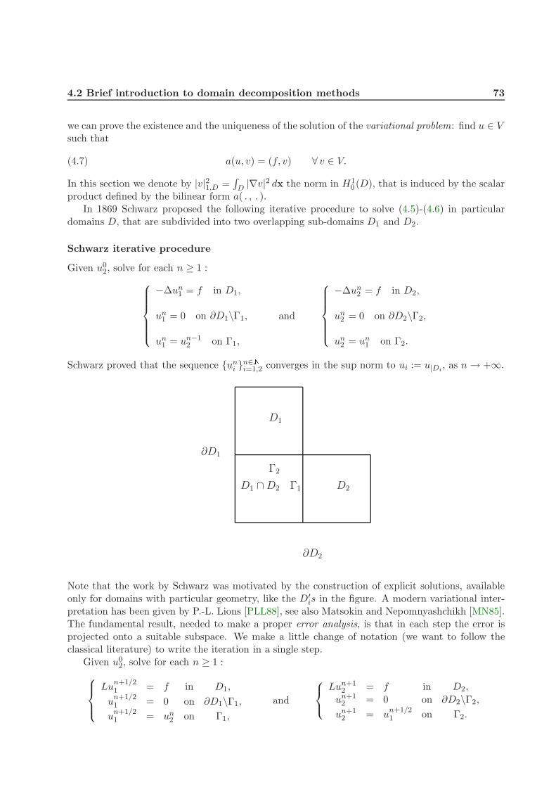
4.2 Brief introduction to domain decomposition methods 73
we can prove the existence and the uniqueness of the solution of the variational problem: find u ∈ Vsuch that
a(u, v) = (f, v) ∀ v ∈ V.(4.7)
In this section we denote by |v|21,D =∫D |∇v|2 dx the norm in H10 (D), that is induced by the scalar
product defined by the bilinear form a( . , . ).In 1869 Schwarz proposed the following iterative procedure to solve (4.5)-(4.6) in particular
domains D, that are subdivided into two overlapping sub-domains D1 and D2.
Schwarz iterative procedure
Given u02, solve for each n ≥ 1 :−∆un1 = f in D1,
un1 = 0 on ∂D1\Γ1,
un1 = un−12 on Γ1,
and
−∆un2 = f in D2,
un2 = 0 on ∂D2\Γ2,
un2 = un1 on Γ2.
Schwarz proved that the sequence uni n∈Ni=1,2 converges in the sup norm to ui := u|Di, as n → +∞.
D2
D1
Γ2
∂D2
Γ1
∂D1
D1 ∩ D2
Note that the work by Schwarz was motivated by the construction of explicit solutions, availableonly for domains with particular geometry, like the D′
is in the figure. A modern variational inter-pretation has been given by P.-L. Lions [PLL88], see also Matsokin and Nepomnyashchikh [MN85].The fundamental result, needed to make a proper error analysis, is that in each step the error isprojected onto a suitable subspace. We make a little change of notation (we want to follow theclassical literature) to write the iteration in a single step.
Given u02, solve for each n ≥ 1 :Lu
n+1/21 = f in D1,
un+1/21 = 0 on ∂D1\Γ1,
un+1/21 = un2 on Γ1,
and
Lun+12 = f in D2,
un+12 = 0 on ∂D2\Γ2,un+12 = u
n+1/21 on Γ2.
74 Domain decomposition methods
By considering the weak formulation in H10 (D), (each function belonging to H10 (Di) is considered,after an extension to zero on D\Di, as a function of H10 (D)) we easily see that the Schwarz iterationis, for n ∈ N, equivalent to
find un+1/2 − un ∈ H10 (D1) : a(un+1/2 − un, v) = (f, v) − a(un, v) ∀ v ∈ H10 (D1),
find un+1 − un+1/2 ∈ H10 (D2) : a(un+1 − un+1/2, v) = (f, v) − a(un+1/2, v) ∀ v ∈ H10 (D2).
If we denote by en the error after n-steps, en := u− un, we have that it satisfies
a(un+1/2 − un, v) = a(en, v) ∀ v ∈ H10 (D1)
anda(un+1 − un+1/2, v) = a(en+1/2, v) ∀ v ∈ H10 (D2).
The analysis above proves the following proposition:
Proposition 4.2.1. In each half-step the Schwarz iteration projects the error onto H10 (Di), i.e.the solution is corrected (no error) in Di. We have in fact that
un+1/2 − un = P1 en with P1 : H10 (D) → H10 (D1),
un+1 − un+1/2 = P2 en+1/2 with P2 : H10 (D) → H10 (D2),
where Pi are the orthogonal projectors defined by the variational problems
find Pi u ∈ H10 (Di) a(Pi u, v) = a(u, v) ∀ v ∈ H10 (Di).
Finite dimensional interpretation
When we pass to a discretization with a finite dimensional space, as in the previous Section 1.4, wecan write the iteration in matrix form. As usual, u will belong to the polynomial space V h ⊂ H10 (D),that we defined in Section 3.1.1. Furthermore A and Ai will be respectively the stiffness matrixrelative to the bilinear form a( . , . ) and to its restrictions to Di
ai(u, v) := a|Di(u, v) :=
∫Di
∇u · ∇v dx.
In matrix form the Schwarz iteration can be written asun+1/2 = un +
(A−11 00 0
)(f −Aun),
un+1 = un+1/2 +(
0 00 A−1
2
)(f −Aun+1/2).
If we now introduce the rectangular matrices Ri, such that Ri applied to v ∈ V h returns the vectorof coefficients defined in the interior of Di, the iteration can be written as
un+1/2 = un + RT1 (R1ART
1 )−1R1(f −Aun),
un+1 = un+1/2 + RT2 (R2ART
2 )−1R2(f −Aun+1/2).
Then, by defining the matrices Bi := RTi (RiAR
Ti )−1Ri, we can use a compact notation.
4.2 Brief introduction to domain decomposition methods 75
MSM-Multiplicative Schwarz method
The multiplicative Schwarz method read as: solve for each m ≥ 0un+1/2 = un + B1(f −Aun),
un+1 = un+1/2 + B2(f −Aun+1/2).
or in a one-step version
un+1 = un + (B1 + B2 −B2AB1)(f −Aun).
The particular form that we used to write the iteration points out clearly as the multiplicativeSchwarz method performs a preconditioned Richardson iterations, with preconditioner
B := B1 + B2 −B2AB1.
It can be easily seen that this preconditioner is exactly the block Gauss-Seidel. The blocks arerelative to the unknowns of Di for i = 1, 2.
ASM-Additive Schwarz Method
It is now natural to consider the block Jacobi preconditioner, to get the additive Schwarz method.Solve for each m ≥ 0 :
un+1 = un + (B1 + B2)(f −Aun).
The preconditioner isB := B1 + B2.
We shall not investigate the properties of these overlapping methods. We only observe that aniterative procedure produces a preconditioner, which can be proved to be optimal, if Vh con-sists of piecewise linear functions. For detailed discussion, see the book by Smith, Bjørstad andGropp [SBG96].
4.2.2 Substructuring methods
In this section we want to introduce the other approach to domain decomposition methods. Weconsider a domain D partitioned into two non-overlapping sub-domains D1 and D2, and we supposethat the interface Γ := D1 ∩D2, which separates them, is a (d− 1)-dimensional Lipschitz manifold.We define again ui := u|Di
and by we denote by ni the outward normal direction on ∂Di ∩ Γ.Moreover, we let n := n1. It is a classical result that the Poisson problem (4.5)-(4.6) in D can bereformulated as follows:
−∆u1 = f in D1,
u1 = 0 on ∂D1 ∩ ∂D,
u1 = u2 on Γ,
∂u2∂n
=∂u1∂n
on Γ,
u2 = 0 on ∂D2 ∩ ∂D,
−∆u2 = f in D2.
(4.8)
76 Domain decomposition methods
The conditions u1 = u2 and ∂u2/∂n = ∂u1/∂n on Γ are known as transmission conditions. We nowdenote by λ the unknown value of u on Γ and, with standard notation, we define wi, for i = 1, 2,by
−∆wi = f in Di,
ui = 0 on ∂Di ∩ ∂D,
ui = λ on Γ,
(4.9)
and we observe that wi = u0i + ui, where u0i and ui are defined by−∆u0i = 0 in Di,
u0i = 0 on ∂Di ∩ ∂D,
u0i = λ on Γ,
−∆ui = f in Di,
ui = 0 on ∂Di ∩ ∂D,
ui = 0 on Γ.
If we compare the problem solved by wi and by ui, we obtain that wi = ui if and only if
∂w1∂n
=∂w2∂n
on Γ.(4.10)
We recall that u0i is the harmonic extension of λ into Di, which will be denoted by Hiλ.
Steklov-Poincare interface equation
The problem in two domains can be written, by recalling the latter condition (4.10) involving thenormal derivative of wi, as a single interface condition. We formally define S, the Steklov-Poincareoperator, as:
Sη :=∂H1η
∂n− ∂H2η
∂n.(4.11)
This operator, which can be split in S := S1+S2, with Si := ∂Hiλ/∂ni, was introduced3 by Steklovand Poincare at the end of the 19th century. If we define Tif := ui and furthermore
χ :=∂T1f
∂n− ∂T2f
∂n,
we can write (4.10), as the following equation satisfied by λ :
Sλ = χ.(4.12)
Variational formulation
The calculations of the previous section were only formal. To properly define the Steklov-Poincareoperators we need a weak formulation of the multi-domain Problem 4.8. In order to do this wedefine:
Vi := vi ∈ H1(Di) : vi|∂D∩∂Di= 0,
V 0i := H10 (Di),Λ := η ∈ H1/2(Γ) : η = v|Γ for some v ∈ V .
(4.13)
3We recall that in the Russian literature it is studied the inverse operator S−1 and it is called Poincare-Steklovoperator.
4.2 Brief introduction to domain decomposition methods 77
Remark 4.2.2. If Γ∩∂D = ∅ then Λ = H1/2(Γ). Moreover, when Γ∩∂D = ∅ the space Λ, usuallydenoted by H
1/200 (Γ), is topologically and algebraically strictly included in H1/2(Γ), see J.-L. Lions
and Magenes [LM72] for further results. Note, in particular, that the following trace inequalityholds:
∃C∗i > 0 such that ‖vi|Γ‖Λ ≤ C∗
i ‖vi‖1,Di ∀ vi ∈ Vi, for i = 1, 2.(4.14)
Finally, for i = 1, 2 denote by Ri any possible (continuous) operator from Λ to Vi that satisfies(Riη)|Γ = η. Any such operator (we can prove that it exists) will be called an extension operatorfrom Λ to Vi.
By using suitable test functions it can be easily proved that the Poisson equation (4.7) can beequivalently reformulated as: find u1 ∈ V1 and u2 ∈ V2 such that
a1(u1, v1) = (f, v1)D1 ∀ v1 ∈ V 01 ,u1 = u2 on Γ,a2(u2, v2) = (f, v2)D2 ∀ v2 ∈ V 02 ,a2(u2,R2µ) = (f,R2µ)D2 + (f,R1µ)D1 − a1(u1,R1µ) ∀µ ∈ Λ,
where Ri denotes any possible extension operator from Λ to Vi.
We can now define properly the Steklov-Poincare operators with a variational formulation.The Steklov-Poincare operator S introduced in (4.11) can be characterized as an operator actingbetween the space of trace functions Λ and its dual Λ′. We apply the Green formula and we recallthat Hiη is the harmonic extension in Di of an η belonging to Λ, for i = 1, 2. We have
〈Sη, µ〉 =2∑
i=1
⟨∂Hiη
∂ni, µ
⟩=
2∑i=1
∫Di
∇Hiη · ∇Riµ = ai(Hiη,Riµ) ∀ η, µ ∈ Λ,
where Ri are the extension operators as in Remark 4.2.2. Hereafter 〈 . , . 〉 denotes the dualitypairing between Λ′ and Λ. In particular, taking Riµ = Hiµ, we obtain the following variationalrepresentation of S:
〈Sη, µ〉 =2∑
i=1
ai(Hiη,Hiµ) ∀ η, µ ∈ Λ,(4.15)
hence the operator S is symmetric. Moreover, from the Poincare inequality, we have that
〈Sη, η〉 =2∑
i=1
‖∇Hiη‖20,Di≥
2∑i=1
11 + C(Di)
|Hiη|21,Di.
By taking into account the trace inequality (4.14), we finally have
〈Sη, η〉 ≥ α‖η‖2Λ ∀ η ∈ Λ,
for a suitable constant α > 0. Therefore S is a coercive operator.Proceeding in an analogous way, from (4.11) we have
〈Siη, µ〉 =∫Di
∇Hiη · ∇Hiµ = ai(Hiη,Hiµ) ∀ η, µ ∈ Λ.
78 Domain decomposition methods
Clearly, each Si is symmetric and furthermore it is coercive:
∃αi > 0 : 〈Siη, η〉 ≥ αi‖η‖2Λ ∀ η ∈ Λ.(4.16)
Another relevant property of the Steklov-Poincare operators Si is that they are continuous:
∃ βi > 0 : 〈Siη, µ〉 ≤ βi‖η‖Λ ‖µ‖Λ ∀ η, µ ∈ Λ.(4.17)
In fact〈Siη, µ〉 ≤ |Hiη|1,Di |Hiµ|1,Di ∀ η, µ ∈ Λ
and, from well known estimates for the solution of elliptic boundary value problems (see, forexample, J.-L. Lions and Magenes [LM72]), it follows that
‖Hiη‖1,Di ≤ C‖η‖Λ ∀ η ∈ Λ.
These properties are of great interest, because they can be used to obtain a numerical solution ofthe Steklov-Poincare interface Problem 4.12. Clearly, as soon as an approximation of λ is available,problem (4.9) can be reduced to the solution of two independent Dirichlet problems.
Finally, we can also give a variational interpretation of the right-hand side χ in (4.12). It canbe expressed through the functions f and Tif as follows:
〈χ, µ〉 = −2∑
i=1
⟨∂Ti∂ni
f, µ
⟩=
2∑i=1
∫Di
(f Riµ−∇Tif · ∇Riµ)
=2∑
i=1
[(f,Riµ)Di − ai(Tif,Riµ)] ∀µ ∈ Λ.
Therefore, the Steklov-Poincare equation (4.12) can be written in the following variational form:
find λ ∈ Λ : 〈Sλ, µ〉 = 〈χ, µ〉 ∀ µ ∈ Λ.(4.18)
From a variational point of view, the functions u0i = Hiλ and ui = Tif, previously introduced, arethe solutions to the following problems:
find Hiλ ∈ Vi : ai(Hiλ, vi) = 0 ∀ vi ∈ V 0i , with Hiλ|Γ = λ.
andfind Tif ∈ V 0i : ai(Tif, vi) = (f, vi) ∀ vi ∈ V 0i .
One possible approach to the solution of (4.18) is to discretize the space Λ and to solve the interfaceequation directly. The variational formulation will use the following spaces
Λh := vh|Γ : vh ∈ Vh,Vi,h := vh|Ωi : vh ∈ Vh,V 0i,h := vh ∈ Vi,h : vh|Γ = 0.
(4.19)
We define the discrete harmonic extension Hi,hη as the solution to
find Hi,hηh ∈ Vi,h : ai(Hi,hηh, vi,h) = 0 ∀ vi,h ∈ V 0i,h, with Hi,hηh|Γ = ηh.
4.2 Brief introduction to domain decomposition methods 79
By using the same arguments that we have shown for the continuous problem, we can define thediscrete Steklov-Poincare operator4 Sh as
〈Shη, µ〉 =2∑
i=1
ai(Hi,hηh,Hi,hµh) =2∑
i=1
〈Si,hηh, µh〉 ∀ ηh, µh ∈ Λh.
It easily turns out that Si,h are both symmetric, continuous and coercive.It should be remarked that the direct approximation of the interface problem is not useful. We
are now reduced to an interface problem with much less unknowns, but the condition number stillbehaves badly, because χ(Sh) - 1/h.
4.2.3 Some iterative methods
In this section we propose some iterative methods, which can be used to solve the interface equation(4.18). The methods, we are going to introduce, are generally known as iterative substructuringmethods. Their main feature is that they have a sub-domain counterpart, defined by solving suitablesequences of Poisson problems. In particular, we introduce the classical Dirichlet-Neumann andNeumann-Neumann methods and we prove that they furnish an optimal preconditioner.
Extension results
Before introducing the methods and the convergence results, we propose two theorems, that arethe core of the convergence results. In particular, with the following two theorems we can see thatthe continuity and coercivity constants of the discrete Steklov-Poincare operators do not dependon h.
Theorem 4.2.3. Let the space Λ be defined as in (4.13) and let Hi be harmonic extension opera-tors. Then there exist two positive constants C1 and C2 such that
C1‖η‖Λ ≤ ‖Hiη‖1,Di ≤ C2‖η‖Λ ∀ η ∈ Λ, for i = 1, 2.(4.20)
The proof is based on the application of the trace inequality (4.14) and classical estimates forthe solution of elliptic problems, see J.-L. Lions and Magenes [LM72].
We now introduce the following theorem, see Bjørstad and Widlund [BW86], Bramble, Pasciakand Schatz [BPS86] and Marini and Quarteroni [MQ89]. It is very important because it statesthat, a finite dimensional level, the constants that bound the harmonic extension of a function, interms of its trace norm, do not depend on h.
Theorem 4.2.4 (Uniform extension theorem). Let D,D1, and D2 be Lipschitz polygonal domains.Let the space Vh := Xh
r ∩H10 (D). Assume that the family of triangulations Th is regular and thatthe family of triangulations Mh, induced by Th on the interface Γ, is quasi-uniform. Then thereexist two positive constants C1 and C2, which depend on the relative sizes of D1 and D2 but areindependent of h, such that
C1‖ηh‖Λ ≤ ‖Hi,hηh‖1,Di ≤ C2‖ηh‖Λ ∀ ηh ∈ Λh for i = 1, 2.(4.21)
4We recall that we can the interpret the discrete Steklov-Poincare operator as the well-known Schur complementmatrix. When the Schur matrix is explicitly computed we have the method known as substructuring. This operationis very expensive and leads to the construction of an ill-conditioned matrix. The iterative methods, we shall present,have the advantage of including a good preconditioner; furthermore, in the sub-domain iteration the Schur matrixshould not be assembled explicitly.
80 Domain decomposition methods
Proof. Since ηh is the trace on the interface Γ of both H1,hηh and H2,hηh, the trace inequality (4.14)states that there exist real positive constants C∗
i such that
‖ηh‖Λ ≤ C∗i ‖Hi,hηh‖1,Di ∀ ηh ∈ Λh for i = 1, 2.
Therefore, the left-hand inequality in (4.21) follows by choosing
C1 := min1/C∗1 , 1/C
∗2.
On the other hand, we have
‖Hi,hηh‖1,Di ≤ ‖Hi,hηh −Hiηh‖1,Di + ‖Hiηh‖1,Di .
From (4.20), it follows that
‖Hiηh‖1,Di ≤ C2‖ηh‖Λ, for i = 1, 2.
Since ηh is a piecewise-polynomial continuous function on Γ and Di is a Lipschitz polygonal domain,the solution Hiηh belongs to H1+s(Di) for some s > 1/2 (see Dauge [Dau88], Corollary 18.15). Foreach r ∈ R we denote by ‖ . ‖r,Di and by ‖ . ‖r,Γ, the norm of the Sobolev spaces Hr(Di) and Hr(Γ),respectively. The following regularity estimate holds:
‖Hiηh‖1+s,Di ≤ C‖ηh‖1/2+s,Γ.
Moreover, we have the finite element error estimate
‖Hi,hηh −Hiηh‖1,Di ≤ Chs‖Hiηh‖1+s,Di ,
which is a consequence of the continuity and coercivity of the bilinear forms ai( . , . ) and of theinterpolation error estimate (see, for example, Ciarlet [Cia78]).
We now use the following inverse inequality5 (see again Ciarlet [Cia78]) to get
hs‖ηh‖1/2+s,Γ ≤ C‖ηh‖Λ ∀ ηh ∈ Λh,
with a constant C independent of h. Therefore, for a suitable constant C2 independent of h weobtain
‖Hi,hηh‖1,Di ≤ C2‖ηh‖Λ.
Remark 4.2.5. We remark that, under the assumptions of the uniform extension theorem thediscrete Steklov-Poincare operators Si,h are continuous and coercive in Λh, uniformly with respectto h.
5Recall that the quasi-uniformity of the mesh on Γ is necessary to have the inverse inequality
‖ηh‖Λ ≤ Ch−1/2
(∫Γ
η2h
)1/2
.
4.2 Brief introduction to domain decomposition methods 81
The Dirichlet-Neumann method
We start by introducing the strong formulation of the Dirichlet-Neumann method. Given λ0, solvefor each k ≥ 0 :
−∆uk+11 = f in D1,
uk+11 = 0 on ∂D1 ∩ ∂D,
uk+11 = λk on Γ,
and
−∆uk+12 = f in D2,
uk+12 = 0 on ∂D2 ∩ ∂D,
∂uk+12
∂n=
∂uk+11
∂non Γ,
with
λk+1 := θuk+12|Γ + (1 − θ)λk,(4.22)
where θ is a positive acceleration parameter.This method6 was considered, among the others, by Bjørstad and Widlund [BW86], Bramble,
Pasciak and Schatz [BPS86] and Marini and Quarteroni [MQ89].The variational formulation of this method is the following:
find uk+11 ∈ V1 : a1(uk+11 , v1) = (f, v1)D1 ∀ v1 ∈ V 01 ,(4.23)
with uk+11 = λk on Γ. Then find uk+12 ∈ V2 such thata2(uk+12 , v2) = (f, v2)D2 ∀ v2 ∈ V 02 ,
a2(uk+12 ,R2µ) = (f,R2µ)D2 + (f,R1µ)D1 − a1(uk+11 ,R1µ) ∀µ ∈ Λ(4.24)
and complete the scheme with (4.22). This scheme is easily interpreted as the following precondi-tioned Richardson method
λk=1 = λk + θS−12 (χ− Sλk).(4.25)
We now give an abstract convergence theorem concerning the Richardson iterations (4.25) forequation (4.12) preconditioned by PDN = S2. The convergence will be proved in the abstract wayproposed in Alonso, Trotta and Valli [ATV98], even if weaker convergence results (strictly regardingsymmetric problems, see Remark 4.2.8) were known till 1986. In the sequel the operators Si, fori = 1, 2, act on the Hilbert space (X, ‖ . ‖X ), and S = S1 + S2.
Theorem 4.2.6. Suppose that
a) S2 is continuous: ∃ β2 > 0 : 〈S2η, µ〉 ≤ β2 ‖η‖X ‖µ‖X ∀ η, µ ∈ X;
b) S2 is coercive: ∃α2 > 0 : 〈S2η, η〉 ≥ α2 ‖η‖2X ∀ η ∈ X;
c) S1 is continuous: ∃ β1 > 0 : 〈S1η, µ〉 ≤ β1 ‖η‖X ‖µ‖X ∀ η, µ ∈ X;
d) there exists a constant κ∗ > 0 : 〈S2η,S−12 Sη〉 + 〈Sη, η〉 ≥ κ∗‖η‖2X ∀ η ∈ X.
6The same method without relaxation (that is, with θ = 1) does not necessarily converge, unless special assump-tions are made about D1 and D2, see Quarteroni and Valli [QV99] §1.
82 Domain decomposition methods
Then for any given λ0 in X and for any θ satisfying 0 < θ < θmax, with
θmax :=κ∗α22
β2(β1 + β2)2,
the sequence defined byλk+1 = λk + θS−1
2 (F − Sλk)
converges in X to the solution of problem
find λ ∈ X : 〈Sλ, µ〉 = 〈F , µ〉 ∀µ ∈ X ′.(4.26)
Proof. We note that the operator S2 is invertible as a consequence of assumption a), b) and of theLax–Milgram lemma. Let us introduce the S2-scalar product
(η, µ)S2 :=12
(〈S2η, µ〉 + 〈S2µ, η〉).
The corresponding S2-norm ‖η‖S2 := (η, η)1/2S2= 〈S2η, η〉1/2 is equivalent to the norm ‖η‖X , because
it satisfies the two inequalities:
α2‖η‖2X ≤ ‖η‖2S2≤ β2‖η‖2X ∀ η ∈ X.
To prove the convergence of the sequence λkk∈N it is sufficient to show that the mapping Tθ fromX into itself:
Tθη := η − θ S−12 Sη
is a contraction with respect to the S2-norm. By assuming that θ ≥ 0, we have
‖Tθη‖2S2= ‖η‖2S2
+ θ2〈Sη,S−12 Sη〉 − θ(〈S2η,S−1
2 Sη〉 + 〈Sη, η〉)
≤ ‖η‖2S2+ θ2
(β1 + β2)2
α2‖η‖2X − θκ∗‖η‖2X .
By setting
Kθ = 1 + θ2(β1 + β2)2
α22− θ
κ∗
β2,
we obtain ‖Tθη‖2S2≤ Kθ‖η‖2S2
. The bound Kθ < 1 holds if 0 < θ < θmax.
Remark 4.2.7. In Theorem 4.2.6, the upper bound θmax, as well as the contraction constant K1/2θ ,
depends only on α2, β1, β2, and κ∗; consequently, the rate of convergence of the preconditionedRichardson iterative procedure in the S2-norm depends only on these parameters.
Remark 4.2.8. If the operator S2 is symmetric, then assumption d) reduces to the coercivity ofS, that is
〈Sη, η〉 ≥ κ∗
2‖η‖2X .
The corollary below follows immediately, by applying Theorem 4.2.6 with X = H1/200 (Γ), F = χ,
S = S, and Si = Si, i = 1, 2. In fact, by (4.16)-(4.17) we have that the Steklov-Poincare operatorssatisfy all the hypotheses of Theorem 4.2.6, with constants independent of h, see Remark 4.2.5
Corollary 4.2.9. The Dirichlet-Neumann method converges at a rate which is independent of h.
4.2 Brief introduction to domain decomposition methods 83
The Neumann-Neumann method
This method was considered by Bourgat, Glowinski, Le Tallec and Vidrascu [BGLTV89], see alsothe paper by Agoshkov and Lebedev [AL85] for an algebraic approach.
In this case, for each k ≥ 0 we have to solve
−∆uk+1i = f in Di,
uk+1i = 0 on ∂Di ∩ ∂D,
uk+1i = λk on Γ,
and
−∆ψk+1i = 0 in Di,
ψk+1i = 0 on ∂Di ∩ ∂D,
∂ψk+1i
∂n=
∂uk+11
∂n− ∂uk+12
∂non Γ,
for i = 1, 2 with
λk+1 := λk − θ(σ1ψk+11|Γ − σ2ψ
k+12|Γ ).(4.27)
As before λ0 is a given datum, θ > 0 is an acceleration parameter while σ1 and σ2 are two positiveaveraging coefficients (whose introduction becomes essential only when dealing with many sub-domains).
Also the Neumann-Neumann can be interpreted, after a weak formulation, as a preconditionedmethod to solve the interface equation (4.12). We have arrive to the following preconditionedRichardson method
λk+1 = λk + θ(σ1S−11 + σ2S
−12 )(F − Sλk).(4.28)
Remark 4.2.10. We recall that if a linear operator A : Λ → Λ′ is continuous and coercive, withcontinuity constant given by β and coercivity constant given by α, then its inverse A−1 : Λ′ → Λexists (by the Lax–Milgram lemma). Moreover, A−1 is continuous with continuity constant given byα−1 and coercive with coercivity constant given by α/β2. Consequently, for each σ1 > 0 and σ2 > 0the Neumann-Neumann preconditioner PNN := (σ1S−1
1 + σ2S−12 )−1 is symmetric, continuous and
coercive in Λ. If denote by βPNNand αPNN
its continuity and coercivity constant, a straightforwardcomputation shows that they are respectively given by
βPNN:=
β21β22
σ1α1β22 + σ2α2β
21
,
αPNN:=
(σ1α1β22 + σ2α2β21)α
21α22
β21β22(α1σ2 + α2σ1)2
.
We present now another abstract theorem, which concerns the preconditioned Richardson iter-ation, based on the preconditioner PNN = (σ1S−1
1 + σ2S−12 )−1, see Quarteroni and Valli [QV99].
As in Theorem 4.2.6, the operators Si, i = 1, 2 act on the Hilbert space (X, ‖ . ‖X ) and S = S1+S2.
Theorem 4.2.11. Assume that both Si are continuous and coercive; that is, for i = 1, 2, we havethat
a) ∃ βi > 0 : 〈Siη, µ〉 ≤ βi ‖η‖X ‖µ‖X ∀ η, µ ∈ X;
b) ∃αi > 0 : 〈Siη, η〉 ≥ αi ‖η‖2X ∀ η ∈ X.
84 Domain decomposition methods
Assume, moreover, that, for any choice of the averaging parameters σ1 > 0 and σ2 > 0, the operatorPNN := (σ1S−1
1 + σ2S−12 )−1 satisfies the condition
c) ∃κ∗ > 0 : 〈PNNη,P−1NNSη〉 + 〈Sη, η〉 ≥ κ∗‖η‖2X ∀ η ∈ X.
Then there exists θ0 > 0 such that for each θ ∈ (0, θ0) and for any given λ0 ∈ X the sequence
λk+1 = λk + θP−1NN (F − Sλk)(4.29)
converges in X to the solution of (4.26).
Proof. We have already pointed out (recall Remark 4.2.10) that, due to assumptions a) and b),the operator PNN : X → X ′ is continuous and coercive. Let us denote by βPNN
and αPNNits
continuity and coercivity constants. We introduce the PNN -scalar product
(η, µ)PNN:=
12
(〈PNNη, µ〉 + 〈PNNµ, η〉),
and the corresponding PNN -norm ‖η‖PNN:= (η, η)1/2PNN
= 〈PNNη, η〉1/2, which is equivalent to thenorm ‖η‖X , i.e. ,
αPNN‖η‖2X ≤ ‖η‖2PNN
≤ βPNN‖η‖2X .
To prove the convergence of λkk∈N, we show that the following map Tθ from X into itself
Tθη := η − θP−1NNSη
is a contraction with respect to the norm ‖ · ‖PNN. By assuming that θ ≥ 0, for η ∈ X we have
‖Tθη‖2PNN= ‖η‖2PNN
+ θ2〈Sη,P−1NNSη〉 − θ(〈PNNη,P−1
NNSη〉 + 〈Sη, η〉)
≤ ‖η‖2PNN+ θ2〈Sη,P−1
NNSη〉 − θκ∗‖η‖2X .
The operator P−1NN = σ1S−1
1 + σ2S−12 is continuous and satisfies
〈ψ,P−1NNψ〉 ≤
(σ1α1
+σ2α2
)‖ψ‖2X′ ∀ψ ∈ X ′,
therefore
〈Sη,PNN−1Sη〉 ≤
(σ1α1
+σ2α2
)(β1 + β2)2‖η‖2X .
By setting
Kθ = 1 + θ2(σ1α1
+σ2α2
)(β1 + β2)2
αPNN
− θκ∗
βPNN
,
we obtain‖Tθη‖2PNN
≤ Kθ‖η‖2PNN.
Finally, by setting
θ0 :=κ∗αPNN
βPNN
(σ1α1
+σ2α2
)(β1 + β2)2
,
we conclude that Tθ is a contraction for all θ ∈ (0, θ0).
4.2 Brief introduction to domain decomposition methods 85
Remark 4.2.12. We observe that the rate of convergence in the PNN -norm of the preconditionedRichardson iterative procedure (4.29) depends only on the constants σ1, σ2, α1, α2, β1, β2, and κ∗.Moreover, if S1 and S2 are symmetric, assumption c) is equivalent to the coercivity of S. On theother hand, this property follows directly from b). Hence, in the symmetric case assumption c) isnot necessary.
Again, by setting X = H1/200 (Γ), F = χ, S = S, and Si = Si, for i = 1, 2, we have the following
result, see Corollary 4.2.9
Corollary 4.2.13. The Neumann-Neumann method converges at a rate which is independent ofh.
The Robin method
We now propose the Robin method, that was introduced and analyzed by P.-L. Lions [PLL90]. Itreads as: given u02, for each k ≥ 0 solve
−∆uk+11 = f in D1,
uk+11 = 0 on ∂D1 ∩ ∂D,
∂uk+11
∂n+ γ1u
k+11 =
∂uk2∂n
+ γ1uk2 on Γ,
and
−∆uk+12 = f in D2,
uk+12 = 0 on ∂D2 ∩ ∂D,
∂uk+12
∂n− γ2u
k+12 =
∂uk1∂n
− γ2uk1 on Γ,
where γ1 and γ2 are two nonnegative acceleration parameters such that γ1+γ2 > 0. We now presentthe proof of convergence in the simplified context of γ1 = γ2 = γ. This reduction greatly simplifiesthe calculations, but leaves unaffected the main idea. Furthermore, we make the calculations in thedifferential context, but the same method can be used to show the convergence of the variationalformulation, both at the infinite-dimensional and discrete level, see Quarteroni and Valli [QV99].
Theorem 4.2.14. If γ1 = γ2 = γ > 0, then the local errors eki := uki − u|Diconverge to zero with
respect to the norm H1(Di), for i = 1, 2.
Proof. The local errors satisfy
−∆ek+11 = 0 in D1,
ek+11 = 0 on ∂D1 ∩ ∂D,
∂ek+11
∂n+ γ1e
k+11 =
∂ek2∂n
+ γ1ek2 on Γ,
and
−∆ek+12 = 0 in D2,
ek+12 = 0 on ∂D2 ∩ ∂D,
∂ek+12
∂n− γ2e
k+12 =
∂ek1∂n
− γ2ek1 on Γ.
We multiply the equation satisfied by ek+12 by ek+12 itself. Then we integrate by parts and we getthat
‖∇ek+12 ‖20,D2= −
∫Γ
∂ek+12
∂nek+12 .
By using the identity AB =1
4γ[(A + γB)2 − (A− γB)2], we can write
−∫Γ
∂ek+12
∂nek+12 =
14γ
∫Γ
(∂ek+12
∂n− γek+12
)2− 1
4γ
∫Γ
(∂ek+12
∂n+ γek+12
)2.
86 Domain decomposition methods
By recalling the boundary condition on Γ satisfied by ek+12 , we obtain
‖∇ek+12 ‖20,D2+
14γ
∫Γ
(∂ek+12
∂n+ γek+12
)2=
14γ
∫Γ
(∂ek+11
∂n− γek+11
)2.
By repeating the same argument for ek+11 , we find that
‖∇ek+11 ‖20,D1+
14γ
∫Γ
(∂ek+11
∂n− γek+11
)2=
14γ
∫Γ
(∂ek2∂n
+ γek2
)2.
Adding the last two equalities and summing over k, from k = 0 to k = M − 1, we obtain that
M∑k=1
(‖∇ek1‖20,D1+ ‖∇ek2‖20,D2
) +1
4γ
∫Γ
(∂eM2∂n
+ γeM2
)2=
14γ
∫Γ
(∂e02∂n
+ γe02
)2.
Consequently, the series on the left hand side is convergent and eki tends to 0 in H1(Di) fori = 1, 2.
Remark 4.2.15. In contrast with the Dirichlet-Neumann and Neumann-Neumann methods, forthe Robin method we do not have estimates regarding the reduction of the error. Furthermore, wedo not have any information about the rate of convergence.
4.3 Non-symmetric problems
In this section we analyze the domain decomposition methods for non-symmetric elliptic equa-tions. When dealing with elliptic equations with first order terms or with non-symmetric principalpart, the theory becomes more difficult. In general no convergence result can be proved, if someassumption linking the “bigness” of non-symmetric part and the dimension of sub-domains arenot assumed. We do not study the problem with overlapping sub-domains. For Schwarz methodsregarding non-symmetric equations, we refer to Cai, Gropp and Keyes [CGK92] and Cai and Wid-lund [CW92]. The study of non-symmetric equation gives new additional problems, as we shall seein the following sections. Particular interface conditions should be used and new method must beintroduced. We consider a non-symmetric elliptic operator of the following form:
Lw := −d∑
l,j=1
∂
∂xl
(alj
∂w
∂xj
)+
d∑j=1
∂(bjw)∂xj
+ a0w.(4.30)
We assume that the coefficients alj are uniformly positive-definite:
∃α0 > 0 :d∑
l,j=1
alj(x)ξjξl ≥ α0|ξ|2 ∀ ξ ∈ Rd, a.e.x ∈ D.
We shall study the homogeneous Dirichlet problem associated with the operator L. When dealingwith the two-domain formulation, the interface condition on Γ are
u1 = u2 on Γ,
∂u1∂nL
=∂u2∂nL
on Γ,or equivalently
u1 = u2 on Γ,
∂u1∂nL
+ γu1 =∂u2∂nL
+ γu2 on Γ,
4.3 Non-symmetric problems 87
where∂u
∂nL:=
d∑l,j=1
alj∂u
∂xjnl
is called the co-normal derivative.
Variational formulation
Let us assume that alj , bj, and a0 belong to L∞(D), for each l, j = 1, . . . , d and that div b belongsto L∞(D). Then we can introduce in H1(D) the continuous bilinear form, associated to L :
a#(w, v) :=∫D
[d∑
l,j=1
alj∂w
∂xj
∂v
∂xl+(
12
div b + a0
)w v
]dx +
12
∫D
(v b · ∇w − w b · ∇v) dx,
Under the further assumption that
12
div b(x) + a0(x) ≥ 0 a.e.x ∈ D,(4.31)
the bilinear form a#(·, ·) is coercive in V = H10 (D). Therefore, the homogeneous Dirichlet boundaryvalue problem: find u ∈ H10 (D) such that
a#(u, v) = (f, v) ∀ v ∈ H10 (D)(4.32)
has a unique solution. By defining in Vi, i = 1, 2, (see page 76) the local bilinear forms
a#i (wi, vi) :=∫Di
[d∑
l,j=1
alj∂wi
∂xj
∂vi∂xl
+
(12
div b + a0
)wivi dx +
12
∫D
(vi b · ∇wi − wi b · ∇vi) dx,
we can define the extension operators E#i : Λ → Vi such that
E#i η ∈ Vi : a#(E#i η, v) = 0 ∀ v ∈ V 0i with E#i η|Λ = η.
With these operators, we can define the Steklov-Poincare operators exactly as for the Laplaceequation
〈Siη, µ〉 = a#i (E#i η,E#i µ) ∀ η, µ ∈ Λ.(4.33)
We have easily that Si are continuous and coercive, i.e. , that (4.16)-(4.17) are satisfied for suitablepositive constants αi and βi. We can formulate an interface problem
find λ ∈ Λ : 〈Sλ, µ〉 = 〈χ, µ〉 ∀ µ ∈ Λ,
which is equivalent to (4.32). In this problem χ is defined by
〈χ, µ〉 =2∑
i=1
[(f,Riµ)Di − a#i (T#i f,Riµ)] ∀µ ∈ Λ
and T#i f solves the following variational problem
find T#i f ∈ V 0i : a#i (T#i f, vi) = (f, vi) ∀ vi ∈ V 0i , for i = 1, 2.
88 Domain decomposition methods
Due to the choice7 of the bilinear form a#( . , . ), the interface condition is:
∂u2∂nL
− 12
b · nu2 =∂u1∂nL
− 12
b · nu1 on Γ.
4.3.1 Results for “slightly” non-symmetric problems
We now give some convergence results for iterative methods corresponding to non-symmetric equa-tions. We shall use the abstract theorems of the previous section and we give some condition whichmake the assumptions to be satisfied, see Quarteroni and Valli [QV99] §5.
Dirichlet-Neumann method
We denote by Dirichlet-Neumann the method that is the counterpart of (4.22)-(4.23)-(4.24), in-troduced for the Laplace equation. In this case we have a Dirichlet problem coupled with a Robinproblem and not a Neumann one as for the Laplace equation.
We claim that if the skew-symmetric part of S2 is small enough, we can prove that conditiond) in Theorem 4.2.6, namely
〈S2η,S−12 Sη〉 + 〈Sη, η〉 ≥ κ∗‖η‖2Λ ∀ η ∈ Λ,
is satisfied (for Si = Si) and then the method converges. We introduce the symmetric and skew-symmetric parts of the bilinear form a#(·, ·), which are given respectively by
as(w, v) :=∫D
[d∑
l,j=1
12
(alj + ajl)∂w
∂xj
∂v
∂xl+(
12
div b + a0
)w v
]dx
ass(w, v) :=∫D
[d∑
l,j=1
12
(alj − ajl)∂w
∂xj
∂v
∂xl+
12
(v b · ∇w − w b · ∇v)
]dx.
Clearly, a# = as + ass. In a similar way we can define the local symmetric and skew-symmetric
7We remark that this is not the only bilinear form (and consequently weak formulation) that can be used. In thepaper by Cai and Widlund [CW92] the different bilinear form
a#(w, v) :=
∫D
[d∑
l,j=1
alj∂w
∂xj
∂v
∂xl+ (a0 + ∇ · b)wv + v b · ∇w
]dx
is used for some technical reasons. This form is obtained without integrating by parts the term[∇ · (bw)
]v. The
following bilinear form is used by adaptive methods
a(w, v) :=
∫D
[d∑
l,j=1
alj∂w
∂xj
∂v
∂xl+ a0wv − wb · ∇v
]dx
and it is obtained integrating by parts[∇ · (bw)
]v, see Carlenzoli and Quarteroni [CQ95] and Gastaldi, Gastaldi
and Quarteroni [GGQ96]. We believe (and numerical experiments confirm it) that in a non overlapping context ourbilinear form a#( . , . ) (that is obtained with “1/2-integration”) is more powerful, since the others can lead to nonsolvable sub-domain problems, see Section 4.4.
4.3 Non-symmetric problems 89
parts asi( . , . ) and assi ( . , . ), for i = 1, 2. By setting µ := S−12 Sη, from (4.33) we have
〈S2η, S−12 Sη〉 + 〈Sη, η〉 = 〈S2η, µ〉 − 〈Sη, η〉 + 2〈Sη, η〉
= 〈S2η, µ〉 − 〈S2µ, η〉 + 2〈Sη, η〉
= as2(E#2 η,E
#2 µ) + ass2 (E#2 η,E
#2 µ) − as2(E
#2 µ,E
#2 η) − ass2 (E#2 µ,E
#2 η)
+ 2〈Sη, η〉
= 2ass2 (E#2 η,E#2 S
−12 Sη) + 2〈Sη, η〉.
By denoting with α the coercivity constant of S, we get
〈S2η, S−12 Sη〉 + 〈Sη, η〉 ≥ 2α‖η‖2Λ − 2|ass2 (E#2 η,E
#2 S
−12 Sη)|.
Therefore, we only have to show that
∃ 0 < ρ < α : |ass2 (E#2 η,E#2 S
−12 Sη)| ≤ ρ ‖η‖2Λ.(4.34)
By settingκssi := max
l,j‖alj − ajl‖L∞(Di) + ‖b‖L∞(Di) for i = 1, 2,
we obtain|ass2 (E#2 η,E
#2 S
−12 Sη)| ≤ C1κ
ss2 ‖E#2 η‖1,D2‖E
#2 S
−12 Sη‖1,D2
≤ C2κss2 ‖η‖Λ‖S−1
2 Sη‖Λ
≤ C3κss2 ‖η‖2Λ.
Then (4.34) follows if
C3κss2 < α,(4.35)
which is a smallness assumption on the skew-symmetric part of the operator L in D2. By applyingTheorem 4.2.6 with Si = Si, for i = 1, 2, we can infer the following result.
Corollary 4.3.1. The Dirichlet-Neumann method converges at a rate which is independent of h,provided (4.35) is satisfied.
Neumann-Neumann method
We consider the analogue of the Neumann-Neumann method for the Poisson equation, even if theiteration steps regarding ψ (see page 83) now involve problems with a Robin-condition on theinterface Γ. We claim that we can use Theorem 4.2.11 if the non-symmetric term is small in bothD1 and D2. In particular, this assumption is necessary to satisfy condition c) :
∃ k∗ > 0 : 〈PNNη,P−1NNSη〉 + 〈Sη, η〉 ≥ κ∗‖η‖2Λ ∀ η ∈ Λ.
In this case PNN = PNN := (σ1S−11 + σ2S
−12 )−1. In fact, by setting µ := P−1
NNSη, we have
〈PNNη, P−1NNSη〉 + 〈Sη, η〉 = 〈PNNη, µ〉 − 〈Sη, η〉 + 2〈Sη, η〉
= 〈PNNη, µ〉 − 〈PNNµ, η〉 + 2〈Sη, η〉.
90 Domain decomposition methods
Moreover, by setting ρi := S−1i PNNη and ξi := S−1
i PNNµ for i = 1, 2, we have
PNNη = S1ρ1 = S2ρ2 and PNNµ = S1ξ1 = S2ξ2,
and consequentlyη = P−1
NNPNNη = σ1ρ1 + σ2ρ2 and µ = σ1ξ1 + σ2ξ2.
Therefore
〈PNNη, µ〉 − 〈PNNµ, η〉 = 〈PNNη, σ1ξ1 + σ2ξ2〉 − 〈PNNµ, σ1ρ1 + σ2ρ2〉
= σ1(〈S1ρ1, ξ1〉 − 〈S1ξ1, ρ1〉) + σ2(〈S2ρ2, ξ2〉 − 〈S2ξ2, ρ2〉)
= 22∑
i=1
σiassi (E#i ρi, E
#i ξi)
= 22∑
i=1
σiassi (E#i S
−1i PNNη,E
#i S
−1i Sη).
We finally obtain that condition c) in Theorem 4.2.11 is satisfied, provided that the constant κssi issmall enough, for i = 1, 2. Hence, by using Theorem 4.2.11 with Si = Si for i = 1, 2, we obtain thefollowing corollary.
Corollary 4.3.2. The Neumann-Neumann method converges at a rate which is independent of h,provided κssi , for i = 1, 2, is small enough
4.3.2 Time-harmonic Maxwell equations
The methods used in the previous section are essentially based on the fact that the operator to bestudied is a small perturbation of a symmetric one. In other problems of classical mathematicalphysics these method are not applicable. In particular, in this section we study the time-harmonicMaxwell equations. This problem is interesting because leads to a complex bilinear form, that iscoervice but not self-adjoint and appropriate techniques must be used. Then we show how thesame analysis of domain decomposition methods applies to the real elliptic equations, to prove ina different and new way the results of Section 4.3.1.
We recall that the Maxwell equations read (recall the definition of curl in Section 1.1.1)∂D∂t
= curlH−J ,
∂B∂t
= −curl E ,
where E and B (which are real, three-dimensional, vector-valued functions of (x, t) ∈ R3 ×R ) arerespectively the electric and magnetic field. Furthermore, D and B are the electric and magneticinduction and J is the current density. We assume the constitutive equations D = ε E and B = µH,where ε is the dielectric constant while µ is the magnetic permeability. We also assume the so-called Ohm law J = σ E , where σ is the electric conductivity. The quantities ε , µ , σ are symmetric
4.3 Non-symmetric problems 91
matrices, which depend on the spatial variable x. We recall that ε and µ are assumed to be uniformlypositive definite, i.e. , there exist two real positive constants C1 and C2 such that:
3∑i,j=1
εij(x)ζiζj ≥ C1|ζ|2 and3∑
i,j=1
µij(x)ζiζj ≥ C2|ζ|2 ∀ ζ ∈ R3, a.e. x ∈ R3.
We also remind that σ is positive definite in a conductor and vanishes in an isolant. For themathematical analysis of the Maxwell equations see Dautray and J.-L. Lions [DL92] Ch. IX; forthe physical meaning of the above equations see Jackson [Jac75].
If we rewrite the equations in terms of E and H, the Maxwell equations becomeε∂E∂t
= curlH− σ E ,
µ∂H∂t
= −curl E .
We consider the time-harmonic problem by looking for solutions of the formE(t,x) = Re
[E(x)ei α t
],
H(t,x) = Re[H(x)ei α t
],
where E and H are complex-valued three-dimensional vectors. Moreover, the complex number iis the imaginary unit and 0 = α ∈ R is a given angular frequency. After rewriting the Maxwellequations in terms of E and H and after substituting in the first equation the expression for Hthat is given from the second equation, we arrive to
curl (µ−1curl E) − α2(ε− iα−1σ)E = 0.
We shall consider the low-frequency problem in which α is “small.” We observe that for a lot ofreal media the term α2ε is much smaller than µ−1 and ασ. It is then physically reasonable to neglectthe term α2εE and, consequently, to study the low-frequency time-harmonic Maxwell equations:
curl (µ−1curl E) + iασE = 0.
When considering the equations in a bounded domain D ⊂ R3, the natural boundary condition isn × E = Ψ on ∂D, where, as usual, n denotes the outward normal vector to ∂D. It is generallyassumed that there exists a vector valued function E such that n× E = Ψ on ∂D. By consideringthe new unknown u := E − E, we can study the following problem
curl (µ−1curl u) + iασ u = f in D,(4.36)(n × u)|∂D = 0 on ∂D,(4.37)
where f := curl (µ−1curl E) + iσα E.
Function spaces and variational formulation
When considering equations (4.36)-(4.37), it is natural to think to a variational formulation in aproper functional space. Clearly, the bilinear form associated to the above problem is given by
a(w,v) :=∫D
(µ−1curl w · curl v + iασw · v) dx.
92 Domain decomposition methods
We need now a precise functional framework because the problem, for its nature, should not betreated in H10 (D). The spaces we shall use are the following ones:
H(curl ;D) :=u ∈ (L2(D))3 : curl u ∈ (L2(D))3
and
H0(curl ;D) :=H(curl ;D) : (n × u)|∂D = 0
,
equipped with the norm
‖u‖2H(curl ;D) = ‖u‖2(L2(D))3 + ‖curl u‖2(L2(D))3 .
For further properties of these spaces, see Girault and Raviart [GR86]. We shall also use, for0 < s ∈ R
Hs(curl ;D) :=u ∈ (Hs(D))3 : curl u ∈ (Hs(D))3
equipped with the norm
‖u‖2Hs(curl ;D) = ‖u‖2(Hs(D))3 + ‖curl u‖2(Hs(D))3 .
We need a knowledge of corresponding trace spaces to properly formulate the problem with twosub-domains, as in the previous sections. We define the tangential divergence of a vector field λ.
Definition 4.3.3. Given λ ∈ (H−1/2(∂D))3 such that (λ · n)|∂D = 0, we define its tangentialdivergence divτλ ∈ H−3/2(∂D) as the distribution such that
〈〈divτλ, ψ〉〉∂D := −〈λ, (∇ψ∗)|∂D〉∂D ∀ψ ∈ H3/2(∂D),
where ψ∗ ∈ H2(D) is any extension of ψ in D. We denote with 〈〈 . , . 〉〉∂D the duality betweenH−3/2(∂D) and H3/2(∂D) and with 〈 . , . 〉∂D that one between H−1/2(∂D) and H1/2(∂D)
We define the Hilbert spaces χ∂D and χΣ, where Σ is a proper subset of ∂D as:
χ∂D :=λ ∈ (H−1/2(∂D))3 : (λ · n)|∂D = 0, divτλ ∈ H−1/2(∂D)
and
χΣ :=λ ∈ (H−1/2(Σ))3 : (λ · n)|Σ = 0, divτ λ ∈ H−1/2(∂D)
,
equipped with the norms
‖λ‖2χ∂D:= ‖λ‖2−1/2,∂D + ‖divτλ‖2−1/2,∂D
and‖λ‖2χΣ
:= ‖λ‖2−1/2,Σ + ‖divτ λ‖2−1/2,∂D,
where λ ∈ (H−1/2(∂D))3 is the extension of λ to 0 on ∂D\Σ.It is well-known, see Alonso and Valli [AV96], that χ∂D and χΣ are algebraically and topologi-
cally equivalent to the spaces of tangential traces of H(curl ;D) and H∂D\Σ(curl ;D), where
H∂D\Σ(curl ;D) :=u ∈ H(curl ;D) : (n × u)|∂D\Σ = 0
.
Furthermore there exist linear and continuous operators R∂D and RΣ such that
R∂D : χ∂D → H(curl ;D), with (n× R∂Dη)|∂D = η
4.3 Non-symmetric problems 93
andRΣ : χΣ → H∂D\Σ(curl ;D), with (n × RΣγ)|Σ = γ.
In the proof of some results we shall need additional regularity. For this reason we define, for0 < s ∈ R
χs∂D :=
λ ∈ (Hs(∂D))3 : (λ · n)|∂D = 0, divτλ ∈ Hs(∂D)
,
with norm‖λ‖2χs
∂D:= ‖λ‖2s,∂D + ‖divτλ‖2s,∂D.
We can now define the notion of weak solution.
Definition 4.3.4. We say that a weak solution to (4.36)-(4.37) is a function u belonging toH0(curl ;D) such that:
a(u,v) = L(v) :=∫D
f · v dx ∀v ∈ H0(curl ;D).
We have the following result, see Leis [Lei79].
Theorem 4.3.5. Let D be a smooth bounded open set of R3 and σ a positive definite matrix. Thenthe bilinear form a( . , . ) is continuous and coercive in H0(curl ;D) and, by using the Lax-Milgramlemma, we can state that there exists a unique weak solution to (4.36)-(4.37).
Two-domain formulation
As we did for the Poisson equations, we now derive a two domain formulation. As usual, we considerthe problem with the domain divided into two sub-domains and we also suppose that µ and σ arepositive constants. We denote by uj, for j = 1, 2, the restriction to Dj of the solution u. It is easyto prove that the following differential problems must be satisfied:
curl (µ−1curl u1) + iασ u1 = f1 in D1,
(n× u1) = 0 on ∂D1\Γ,
(n× u1) = (n × u2) on Γ,
(n× curl u1) = (n × curl u2) on Γ,
(n× u2) = 0 on ∂D2\Γ,
curl (µ−1curl u2) + iασ u2 = f2 in D2.
We set now
Vj :=vj ∈ H(curl ;Dj) : (n× vj)|∂Dj\Γ = 0
= H0(curl ,Dj),
aj(w,v) :=∫Dj
(µ−1curl wj · curl vj + iασ wj · vj) dx,
Lj(vj) :=∫Dj
f · vj dx.
94 Domain decomposition methods
The variational formulation of the problem with two sub-domains is then: find (u1,u2) ∈ V1 × V2such that
a1(u1,v1) = L1(v1) ∀v1 ∈ H0(curl ;D1),
(n × u1)|Γ = (n × u2)|Γ,
a2(u2,v2) = L2(v2) + L1(R1(n × v2)|Γ) − a1(u1,R1(n× v2)|Γ) ∀v2 ∈ V2,
where R1 : χΓ → V1 is any continuous extension operator.
Finite dimensional formulation
We now approximate the Maxwell equations (4.36)-(4.37) with the first-kind Nedelec finite elementsNk
h , but we could use as well the other Nedelec spaces. We recall that these spaces, introducedby Nedelec [Ned80, Ned86], are the natural ones in the finite element approximation of Maxwellequations. We suppose that Dj ⊂ R
3 is a polyhedra with Lipschitz boundary and we supposethat Thh>0 is a regular subdivision of D, made with tetrahedra of diameter less than h. Wealso suppose that each element of Th intersects only D1 or D2 and that Thh>0 induce on Γ aquasi-uniform triangulation Mh. To construct the finite element approximant we define
Nkj,h :=
vh ∈ H(curl ;Dj) : vh|K ∈ Rk, ∀K ∈ Tj,h with Tj,h = Th ∩Dj
,
whereRk := (Pk−1)3 ⊕ Sk.
We denoted by Pk := P 3k , for k ≥ 1, the space of polynomials with degree equal or less than k andby Sk the following space
Sk :=p ∈ (Pk)3 : p(x) · x = 0
,
where Pk ⊂ Pk is the space of homogeneous polynomials of degree k.We also define
Vj,h := Nkj,h ∩ Vj,
V 0j,h := Nkj,h ∩H0(curl ;Dj),
χΓ,h :=
(n× v1,h)|Γ : v1,h ∈ V1,h
=
(n× v2,h)|Γ : v2,h ∈ V2,h.
The finite dimensional problem is: find (u1,h,u2,h) ∈ V1,h × V2,h such that
a1(u1,h,v1,h) = L1(v1,h) ∀v1,h ∈ V 01,h,
(n × u1,h)|Γ = (n × u2,h)|Γ,
a2(u2,h,v2,h) = L2(v2,h) + L1(R1(n × v2,h)|Γ) − a1(u1,h,R1(n × v2,h)|Γ) ∀v2,h ∈ V2,h.
(4.38)
Extension and Steklov-Poincare operators
To properly formulate the interface problem with the Steklov-Poincare operators we define, forevery γh ∈ χh,Γ, the extension Eh
j,Γγh which is solution of the problem: find Ehj,Γγh ∈ Vj,h such
thataj(Eh
j,Γγh,vj,h) = 0 ∀vj,h ∈ V 0j,h, with (n × Ehj,Γγh)|Γ = γh.
4.3 Non-symmetric problems 95
We denote by uj,h ∈ V 0j,h the solution of the problem
find uj,h ∈ V 0j,h : aj(uj,h,vj,h) = Lj(vj,h) ∀vj,h ∈ V 0j,h.
The existence and uniqueness of Ehj,Γγh and uj,h are a consequence of the Lax-Milgram lemma.
The couple (Eh1,Γλh + u1,h,Eh
2,Γλh + u2,h) is solution of (4.38) if and only if the following equalityis satisfied
a2(Eh2,Γλh + u2,h,v2,h) = L2(v2,h) + L1(Eh
1,Γ(n× v2,h)|Γ)
−a1(Eh1,Γλh + u1,h,Eh
1,Γ(n × v2,h)|Γ) ∀v2,h ∈ V2,h.
By using the extension operators Ehj,Γ we have that the previous equation is equivalent to
a2(Eh2,Γλh,E
h2,Γµh) + a2(u2,h,Eh
2,Γµh) = L2(Eh2,Γµh) + L1(Eh
1,Γµh)
−a1(Eh1,Γλh,E
h1,Γµh) − a1(u1,h,Eh
1,Γµh) ∀µh ∈ χΓ,h.(4.39)
We can now define the Steklov-Poincare operators Sj,hj=1,2 as follows
〈〈 Sj,hγh,µh 〉〉h := aj(Ehj,Γγh,E
hj,Γµh) ∀γh,µh ∈ χΓ,h,
where 〈〈 . , . 〉〉h is the duality between χΓ,h and (χΓ,h)′. We also define the operator Φh from χΓ,hinto its dual space (χΓ,h)′ by
〈〈Φh,µh 〉〉h := L1(Eh1,Γµh) − a1(u1,h,Eh
1,Γµh) + L2(Eh2,Γµh) − a2(u2,h,Eh
2,Γµh) ∀µh ∈ χΓ,h.
Interface Problem
Problem 4.38 (and consequently 4.39) can be seen as the following interface problem. In theinterface spaces we have to find λh ∈ χΓ,h such that
〈〈 (S1,h + S2,h)λh,µh 〉〉h = 〈〈Φh,µh 〉〉h ∀µh ∈ χΓ,h.(4.40)
The operators Sj,h are continuous and coercive in χΓ,h and, to solve problem (4.40), we use boththe “Dirichlet-Neumann” and the “Neumann-Neumann” procedure8. We apply the Richardsonmethod, with preconditioners that are respectively:
Ph,DN := S−12,h and Ph,NN :=
(S−11,h + S−1
2,h
)−1.
The analysis of the convergence of the Dirichlet-Neumann method has been provided by Alonsoand Valli [AV99]; that one of the Neumann-Neumann method is due to Berselli [Ber99].
8We use the same terminology of the previous sections, even if the boundary conditions are not of Dirichlet orNeumann type. See the differential interpretation.
96 Domain decomposition methods
Dirichlet-Neumann method
We have the following iterative method: given λ0h ∈ χΓ,h, for each m ≥ 0 solve
λm+1h = λmh + θ S−12,h [Φh − (S1,h + S2,h)λmh ] = (1 − θ)λmh + θ S−1
2,h [Φh − S1,hλmh ] .(4.41)
With an argument similar of that of the previous sections, we have that (4.41) is equivalent to thefollowing sub-domain iteration: given λ0h ∈ χΓ,h, for each m ≥ 0 find um+1
1,h ∈ V1,h such that
a1(um+11,h ,v1,h) = L1(v1,h) ∀v1,h ∈ V 01,h with (n× um+1
1,h )|Γ = λmh .
Then find um+12,h ∈ V2,h such that
a2(um+12,h ,v2,h) = L2(v2,h) + L1(Eh
1,Γ(n × v2,h)|Γ) − a1(um+11,h ,Eh
1,Γ(n × v2,h)Γ) ∀v2,h ∈ V2,h
and finally
λm+1h = (1 − θ)λmh + θ(n× um+12,h )|Γ.(4.42)
This procedure is the finite dimensional variational formulation of the Dirichlet-Neumann iteration,relative to problem (4.36)-(4.37). In a strong formulation the continuous problem reads as: for eachm ≥ 0, find um+1
j such thatcurl (µ−1curl um+1
1 ) + iασ um+11 = f1 in D1,
n × um+11 = 0 on ∂D1 ∩ ∂D,
n × um+11 = λmh on Γ,
and curl (µ−1curl um+1
2 ) + iσαum+12 = f2 in D2,
n × um+12 = 0 on ∂D2 ∩ ∂D,
n × curl um+12 = n× curl um+1
1,h on Γ,
completed with condition (4.46).
Neumann-Neumann method
We now describe the second method of this section. We have the following iterative method. Givenλ0h ∈ χΓ,h, for each m ≥ 0 solve
λm+1h = λmh + θ (S−11,h + S−1
2,h) [Φh − (S1,h + S2,h)λmh ] .(4.43)
With a standard argument, we have that (4.43) is equivalent to the following sub-domain iteration:given λ0h ∈ χΓ,h, for every m ≥ 0, find um+1
j,h such that
aj(um+1j,h ,vj,h) = Lj(vj,h) ∀vj,h ∈ V 0j,h,
4.3 Non-symmetric problems 97
with (n × um+1j,h )|Γ = λmh , then find ψk+1
1,h ∈ V1,h such thata1(ψk+1
1,h ,v1,h) = 0 ∀v1,h ∈ V 01,h
a1(ψk+11,h ,R1γh) = −L1(R1γh) − L2(R2γh)
+a1(uk+11,h ,R1γh) + a2(uk+1
2,h ,R2γh) ∀γh ∈ χΓ,h,
(4.44)
then find ψk+12,h ∈ V2,h such that
a2(ψk+12,h ,v2,h) = 0 ∀v2,h ∈ V 02,h
a2(ψk+12,h ,R2γh) = L1(R1γh) + L2(R2γh)
−a1(uk+11,h ,R1γh) − a2(uk+1
2,h ,R2γh) ∀γh ∈ χΓ,h,
(4.45)
with
λm+1h = λmh − θ[(n ×ψm+1
1,h )|Γ − (n ×ψm+12,h )|Γ
].(4.46)
This procedure is the variational formulation of the Neumann-Neumann iteration, relative to prob-lem (4.36)-(4.37), which is written (in a strong formulation) as
curl (µ−1curl um+1j ) + iασ um+1
j = fj in Dj,
n× um+1j = 0 on ∂Dj ∩ ∂D,
n× um+1j = λmh on Γ,
and
curl (µ−1curlψm+1j ) + iσαψm+1
j = 0 in Dj ,
n ×ψm+1j = 0 on ∂Dj ∩ ∂D,
n × curlψm+1j = n× curl um+1
1 − n× curl um+12 on Γ,
completed with condition (4.46).
A convergence result
We now state an abstract result. We shall use this proposition to prove the convergence, with arate which does not depend9 on h, of the Richardson methods (4.41) and (4.43).
Proposition 4.3.6. Let X be a complex Hilbert space and let Sj,h : Xh +→ X ′h for j = 1, 2 be two
linear operators with Xh ⊂ X and dim Xh < +∞. Furthermore, let πs, s = 1, . . . ,Mh be a basis ofXh. We define the matrices Sj,h associated to the operators Sj,h as
(Sj,hγ,µ)h := 〈〈 Sj,hγh,µh〉〉h ∀γ,µ ∈ CMh , j = 1, 2,
9We observe that, in the following, the constants that bound the eigenvalues do not depend on h.
98 Domain decomposition methods
where ( . , . )h denotes the Euclidean scalar product in CMh . Finally, let
γh :=Mh∑s=1
γs πs and µh :=Mh∑s=1
µs πs.(4.47)
Let us suppose that there exist αj , βj > 0 for j = 1, 2, independent of h, such that
|〈〈 Sj,hγh,µh 〉〉h| ≤ βj‖γh‖X‖µh‖X ∀γh,µh ∈ Xh for j = 1, 2,(4.48)
|〈〈 Sj,hγh,γh〉〉h| ≥ αj‖γh‖2X ∀γh ∈ Xh for j = 1, 2,(4.49)
Re〈〈 Sj,hγh,γh〉〉h Re〈〈 S [j],hγh,γh〉〉h +
+ Im〈〈 Sj,hγh,γh〉〉h Im〈〈 S [j],hγh,γh〉〉h ≥ 0 ∀γ ∈ Xh,(4.50)
where
[j] =
2 if j = 1,1 if j = 2.
Then if νj,h = ν1j,h + iν2j,h ∈ C, with νij,h ∈ R for i, j = 1, 2, is an eigenvalue of S−1[j],hSj,h, we have
that
ν1j,h ≥ 0 and |νj,h|2 =|〈〈 Sj,hγh,γh〉〉h|2∣∣〈〈 S [j],hγh,γh〉〉h∣∣2 ≤
(βjα[j]
)2.
Proof. If νj,h is an eigenvalue of S−1[j],hSj,h, then the corresponding eigenvector 0 = γ ∈ RMh satisfies
Sjhγh = νj,h S[j],hγ
and consequently〈〈 Sj,hγh,γh〉〉h = νj,h 〈〈 S [j],hγh,γh〉〉h,
where γh is defined in (4.47). Since νj,h = ν1j,h + i ν2j,h we have
Re 〈〈 Sj,hγh,γh〉〉h = ν1j,h Re 〈〈 S [j],hγh,γh〉〉h − ν2j,h Im 〈〈 S [j],hγh,γh〉〉h,(4.51)
Im 〈〈 Sj,hγh,γh〉〉h = ν1j,h Im 〈〈 S [j],hγh,γh〉〉h + ν2j,h Re〈〈 S [j],hγh,γh〉〉h.(4.52)
By multiplying the two equations (4.51)-(4.52) by Re〈〈 S [j],hγh,γh〉〉h and by Im〈〈 S [j],hγh,γh〉〉h,respectively and by summing up we obtain
ν1j,h
[(Re 〈〈 S [j],hγh,γh〉〉h
)2 +(Im 〈〈 S [j],hγh,γh〉〉h
)2] = Re 〈〈 Sj,hγh,γh〉〉h··Re 〈〈 S [j],hγh,γh〉〉h + Im 〈〈 Sj,hγh,γh〉〉hIm 〈〈 S [j],hγh,γh〉〉h.
(4.53)
From (4.49) we obtain |〈〈 Sj,hγh,γh〉〉h| = 0 and from (4.50) we get ν1j,h ≥ 0.From (4.48)-(4.49) we also obtain
|νj,h|2 =|〈〈 Sj,hγh,γh〉〉h|2∣∣〈〈 S [j],hγh,γh〉〉h∣∣2 ≤
(βjα[j]
)2.
4.3 Non-symmetric problems 99
We observe that if the operators Sj,h are the Steklov-Poincare operators associated to the low-frequency time-harmonic Maxwell equations (4.36)-(4.37), then the hypotheses of Proposition 4.3.6are satisfied. We have that
Re〈〈 Sj,hγh,γh〉〉h =∫Dj
µ−1|curl Ehj,Γγh|2 dx
andIm 〈〈 Sj,hγh,γh〉〉h = α
∫Dj
σ|Ehj,Γγh|2 dx,
and (4.50) holds.By using the following trace10 inequality, see Alonso and Valli [AV96], we have
‖(n × v)|Γ‖2χΓ≤ C∗‖v‖2
H(curl ;Dj)for j = 1, 2.
We can now prove (4.49) by observing that
|〈〈Sj,hγh, γh〉〉h| ≥ C(‖Eh2,Γγh‖2L2(Dj)
+ ‖curl Eh2,Γγh‖2L2(Dj)
)≥ C
C∗ ‖γh‖2χΓ
.
The last condition (4.48) is the most technical to check. This condition is based on the (uniformin h) continuity of the operator Eh
j,Γ. We define kj := sj − 1/2 with sj such that H1+sj(Dj) givesthe best regularity for the solutions of the Laplace problem (in the domain Dj) with homogeneousDirichlet or Neumann boundary conditions and with right hand side in L2(Dj). To prove (4.48) weuse the following lemmas, that are proved in Alonso and Valli [AV99]. These results are based onsome regularity results by Amrouche, Bernardi, Dauge and Girault [ABDG98].
Lemma 4.3.7. Given δ ∈ (0, kj ], there exist R 6 B1,j > 0 for j = 1, 2, such that ∀γ ∈ χΓ withγ ∈ χδ
∂Djwe have Ej,Γγ ∈ H1/2+δ(curl ;Dj) and
‖Ej,Γγ‖H1/2+δ(curl ;Dj)≤ B1,j‖γ‖χδ
∂Dj
for j = 1, 2.
Lemma 4.3.8. Let Th be a regular triangulation and let be given γh ∈ χΓ,h with Ej,Γγh belongingto Ht(curl ;Dj) for t ∈ (1/2, 1). Then there exist R 6 B2,j > 0 for j = 1, 2, independent of h, suchthat
‖Ej,Γγh − Ehj,Γγh‖H(curl ;Dj)
≤ B2,j ht‖Ej,Γγh‖Ht(curl ;D) ∀γh ∈ χΓ,h for j = 1, 2.
Lemma 4.3.9. Let Mh be a quasi-uniform triangulation on ∂Dj induced by Th. Then for everyη ∈ (0, 1/2) there exist R 6 B3,j > 0 for j = 1, 2, independent of h, such that
‖γ‖χη∂Dj
≤ B3,jh−1/2−η‖γ‖χΓ
∀γh ∈ χΓ,h for j = 1, 2.
With the above lemmas we can prove the following proposition, which concludes the verificationof the hypotheses of Proposition 4.3.6.
Proposition 4.3.10. There exist R 6 B4,j > 0 for j = 1, 2, independent of h, such that
|〈〈 Sj,hγh,µh 〉〉h| ≤ B4,j‖γh‖χΓ‖µh‖χΓ
∀γh,µh ∈ χΓ,h for j = 1, 2.
10It is the counterpart of the trace inequality (4.14) that we have seen in the H1(D) framework.
100 Domain decomposition methods
Proof. By using the definition of the Steklov-Poincare operators, we have
|〈〈 Sj,hγh,µh 〉〉h| ≤∣∣∣aj(Eh
j,Γγh,Ehj,Γµh)
∣∣∣ ≤ dj‖Ehj,Γγh‖H(curl ;Dj)
‖Ehj,Γµh‖H(curl ;Dj)
,
where dj is the continuity constant of aj( . , . ). We prove that for j = 1, 2 there exist positiveconstants Cj, which are independent of h, such that
‖Eh1,Γγh‖H(curl ;Dj)
≤ C‖γh‖χΓ∀γh ∈ χΓ,h.
We have
‖Ehj,Γγh‖H(curl ;Dj)
≤ ‖Ehj,Γγh − Ej,Γγh‖H(curl ;Dj)
+ ‖Ej,Γγh‖H(curl ;Dj).
The last term can be bounded by observing that the operator Ej,Γ : χΓ → Vj is continuous. Sinceγh ∈ χΓ,h, we have that γh ∈ χδ
∂Djfor 0 < δ < 1/2. This fact holds because γh and its tangential
divergence are piecewise polynomials. By using Lemma 4.3.7, we have that Ej,Γγh belongs toH1/2+δ(curl ;Dj) for each δ ∈ (0, kj ].
By applying the results of Lemma 4.3.8 with t = 1/2 + δ, we obtain
‖Ehj,Γγh − Ej,Γγh‖H(curl ;Dj)
≤ B2,jh1/2+δ‖Ej,Γγh‖H1/2+δ(curl ;Dj)
≤ B1,jB2,jh1/2+δ‖γh‖χδ
∂Dj
.
By using Lemma 4.3.9 with η = δ, we finally have
‖Ehj,Γγh − Ej,Γγh‖H(curl ;Dj)
≤ B1,jB2,jB3,j‖γh‖χΓ.
We can now prove the convergence of the two preconditioned Richardson methods we introduced. Inparticular we shall prove that spectral radius of the iteration matrix is less than one, or equivalentlythat condition (4.4) is satisfied.
Theorem 4.3.11. There exists a positive constant CDN , not depending on h, such that the precon-ditioned Richardson methods (4.41) (corresponding to the “Dirichlet-Neumann” method) convergesfor any 0 < θ < CDN . Furthermore, there exists a positive constant CNN , not depending on h, suchthat the preconditioned Richardson methods (4.43) (corresponding to the “Neumann-Neumann”method) converges for any 0 < θ < CNN .
Proof. If λh is an eigenvalue of S−12,h(S1,h + S2,h) = I + S−1
2,hS1,h we can write λh = 1 + ν1,h, whereν1,h is an eigenvalue of S−1
2,hS1,h. If γ denotes the corresponding eigenvector we have
〈〈S1,hγh,γh〉〉h = ν〈〈S2,hγh,γh〉〉h.
By using Proposition 4.3.6 we have that
2Reλh|λh|2
= 21 + ν11,h
1 + 2ν11,h + |ν1,h|2≥
1 + ν11,h1 + 2ν11,h + β21/α
22
.
We now observe that the real function
φ(ξ) := 21 + ξ
1 + 2ξ + C21/C22
,
4.3 Non-symmetric problems 101
defined for ξ ≥ 0, is strictly increasing for C1 > C2, strictly decreasing for C2 > C1 and constantlyequal to one for C1 = C2. Moreover, we have that
φ(0) =2C22
C11 + C22and lim
ξ→+∞φ(ξ) = 1.
It follows thatinf
0≤ξ<∞φ(ξ) := CDN > 0.
We have that, for the positive constant CDN , each eigenvalue of S−12,h(S1,h + S2,h) satisfies
2Reλh|λh|2
≥ CDN
and the preconditioned Richardson method (4.41) converges with a rate independent of h, for any0 < θ < CDN .
We pass now to the study of the second method we proposed. We make the following obser-vation: let be given A ∈ GL(n × n,C) (invertible-n× n-complex matrix). Then the eigenvalues ofA + A−1 are of the form:
λ +1λ,
with λ eigenvalue of A. This result easily follows by using the Jordan canonical form. We recallthat there exists a non-singular Q ∈ GL(n × n,C) such that QAQ−1 is in the Jordan canonicalform, i.e. , QAQ−1 is a block diagonal matrix with diagonal blocks of the form
λj 1 0 0 0
0. . . . . . . . . 0
0. . . . . . . . . 0
0. . . . . . . . . 1
0 0 0 0 λj
,
corresponding to each eigenvalue λj. We observe that(QAQ−1)−1 is an upper triangular matrix
and each diagonal block, relative to the eigenvalue µj = 1/λj , is of the form1λj
∗ ∗
0. . . ∗
0 0 1λj
and it has the same dimension of the block relative to the eigenvalue λj of the matrix A. Writtenin the Jordan basis (the basis relative to the canonical form), the sum of QAQ−1 and its inverse(QAQ−1)−1 is an upper-triangular block-matrix with the elements λj +1/λj on the diagonal. Thisproves the observation.
We can now prove the convergence of the preconditioned Richardson methods (4.43). If λh isan eigenvalue of
(S−11,h + S−1
2,h)(S1,h + S2,h) = 2 I + S−11,hS2,h + S−1
2,hS1,h,
it can be written as 2 + νh, where νh is eigenvalue of S−11,hS2,h + S−1
2,hS1,h. Then νh can be written,due to the previous observation, as
νh := ν1,h + ν2,h,
102 Domain decomposition methods
where νj,h is an eigenvalue of S−1[j],hSj,h. By using the results of Proposition 4.3.6 for the eigenvalues
of S−1[j],hSj,h we have
2Reλh|λh|2
= 22 + ν11,h + ν12,h
4 + 4(ν11,h + ν12,h) + |νh|2≥ 2
2 + ν11,h + ν12,h4 + 4(ν11,h + ν12,h) + C
,
because|νh|2 ≤ (|ν1,h| + |ν2,h|)2 ≤ (α1/β2 + α2/β1)2 = C.
We easily obtain that the real function Φ(ξ) := 2(2 + ξ)/(4 + 4 ξ + C) is such that
infξ≥0
Φ(ξ) = min(
44 + C
, 1)> 0.
Since ν1j,h ≥ 0 for j = 1, 2, we have that each eigenvalue λh of (S−11,h + S−1
2,h)(S1,h + S2,h) satisfy
2Reλh|λh|2
≥ CNN ∀ s = 1, . . . ,Mh,
with
CNN := min(
1,4
4 + C
)where C = (α1/β2+α2/β1)2. Consequently the preconditioned Richardson method (4.43) convergeswith a rate which does not depend on h, for every θ ∈ (0, CNN ).
An application to advection diffusion equations
The method that we introduced for the Maxwell equations, can be used to prove in an alternativeway the convergence of the Dirichlet-Neumann and Neumann-Neumann methods for non-symmetricelliptic equations of Section 4.3. We consider the partial differential operator (4.30) with realcoefficients. Its discretization, with the finite element method (or any other), leads to a positive-definite non-symmetric real matrix A. To study the eigenvalues of the iteration matrix for both theDirichlet-Neumann and Neumann-Neumann problem, we complexify the problem. We consider A(denoted by AC) as a linear operator from C
n into itself. We easily see that, if we set u := u1+ iu2and f := f1+i f2, the real part u1 of the solution of ACu = f is exactly the solution of the original realproblem Ax = f1. This approach corresponds to a variational formulation with the non-Hermitiancomplex bilinear form
aC(w, v) :=∫D
[d∑
l,j=1
alj∂w
∂xj
∂v
∂xl+(
12
div b + a0
)w v
]dx +
12
∫D
(v b · ∇w − wb · ∇v) dx.
Observe that the coefficients alj , bl and a0 are still real. To better understand the result, we supposethat alj = ajl and we isolate the non-symmetries of the problem in the first order terms. The realpart of aCi (u, u) (with obvious meaning it is the restriction to Di) is positive for i = 1, 2. Concerningthe complex part, it is easy to check that it is small, provided the quantities ‖bi‖∞ are small. Itholds because the expression of the imaginary part of aCi (u, u) is
12
∫Di
(ub · ∇u− ub · ∇u) dx =12
∫Di
(ub · ∇u− u b · ∇u
)dx.
4.4 Advection diffusion equations and systems 103
Then easy calculation show that condition (4.50) is satisfied provided the modulus of the non-symmetric part is small enough. In this way we proved with a different method the convergence ofthe two classical substructuring methods, if the operator L is a “small” perturbation of a symmetricone. We also remark that the first method, which is based on a contraction argument, givesinformation on the specific norm with respect to convergence is achieved; the second method statesthat the spectral radius is smaller than one and this gives bound for every norm, at a finitedimensional level. In particular, for at least one case the norm of the iteration matrix is small thanone.
4.4 Advection diffusion equations and systems
In this section we analyze again the non-symmetric operator (4.30). In particular we want to findconvergence results or effective methods for equations with “big” non-symmetric terms. We proposesome methods, based on coercivity, which work for equation as well for systems. We recall thatthis problem has been studied with some different domain decomposition methods. In particular weshall explain that big difficulties arise in applying the abstract contraction theorems of the previoussection, because some control on the non-symmetric part is needed.
By using a terminology taken from physics, we call the non-symmetric equation associate tothe operator L of (4.30) advection-diffusion equations. It is clear that the second order term, ordiffusive term, is that one which regularizes the solution. The advection term, which correspondsto the non-symmetric part, is that one which takes into account of “hyperbolic-type” phenomena.The equation, that we consider, is the basic one to be solved in the (first step of) Chorin-Temammethod (recall Section 1.4.3). We observe that the advection-diffusion equations are themselvesan important numerical problem, because just in the one-dimensional case big stability problemsarise, see Quarteroni and Valli [QV94], Ch. 8. In particular, by recalling the results of Chapter 1,we observe that the “bigness” of the non-symmetric part (relative to the symmetric part) dependson the Reynolds number R. In real industrial problems the assumption of smallness of R are highlyunrealistic and the approximate solution of flows at high Reynolds numbers is one of the mostchallenging problems in CFD, computational fluid dynamics. We propose the methods introducedby Berselli and Saleri [BS99] and that one by Alonso, Trotta and Valli [ATV98], together with theanalysis of a new method.
To avoid inessential calculation we assume the second order part to be symmetric and we study,for ε > 0, the following Dirichlet problem
Lεu := −ε∆u +d∑
j=1
∂(bju)∂xj
+ a0u = f in D,(4.54)
u = 0 on ∂D.(4.55)
We assume the same regularity hypotheses of the previous Section 4.3 on bi, i = 1, . . . , d, and a0.Furthermore, we assume condition (4.31), to make the problem coercive.
4.4.1 Adaptive methods
For the sake of completeness, we recall some methods for advection diffusion equations. In thefirst papers regarding domain decomposition methods for non-symmetric equations there whereproposed some methods that should be consistent with the hyperbolic limit: ε → 0. In the papersby Carlenzoli and Quarteroni [CQ95] and Gastaldi, Gastaldi and Quarteroni [GGQ96] there were
104 Domain decomposition methods
proposed the so called adaptive methods. These methods are based on the observation that, tobe consistent with the hyperbolic limit, a Dirichlet condition must not be imposed on outflowboundary , whereas Neumann interface condition has to be enforced at the same boundary. Werecall that the outflow boundary ∂Dout of a domain D is defined by
∂Dout := x ∈ ∂D : b(x) · n(x) > 0,
while the inflow boundary ∂Din is
∂Din := x ∈ ∂D : b(x) · n(x) < 0.
We now present two methods, without stating the convergence results, for which we refer to thepapers cited above or to Quarteroni and Valli [QV99] Ch. 6 §3.
The ADN-adaptive Dirichlet-Neumann method reads as: given u0i in Di, for i = 1, 2, solve foreach k ≥ 0
Lεuk+11 = f in D1,
uk+11 = 0 on ∂D ∩ ∂D1,
uk+11 = λk on Γin ∪ Γ0,
ε∂uk+11
∂n= ε
∂uk2∂n
on Γout,
and
Lεuk+12 = f in D2,
uk+12 = 0 on ∂D ∩ ∂D2,
uk+12 = µk+1 on Γout,
ε∂uk+12
∂n= ε
∂uk+11
∂non Γin ∪ Γ0,
with
λk := θ′uk2|Γin∪Γ0 + (1 − θ′)uk1|Γin∪Γ0 on Γin ∪ Γ0
and
µk+1 := θ′′uk+11|Γout + (1 − θ′′)uk2|Γout on Γout,
where
∂D0 := x ∈ ∂D : b(x) · n(x) = 0.
We recall that θ′ and θ′′ are two positive parameters, that are used to allow possible under-relaxation(if needed) to ensure convergence. It is also possible to introduce the ARN adaptive Robin-Neumannmethod, that is very similar: on each sub-domain iteration the Dirichlet interface condition isreplaced with a Robin one. We observe that these methods need the knowledge (often non easilyavailable) of the inflow and outflow regions. Furthermore it is very difficult to apply these methodsin a vector equation, as the one we want to study.
Some very recent results on substructuring methods are that one proposed by Achdou and Nataf[AN97] and Achdou, Nataf, Le Tallec and Vidrascu [ANLTV98]. In these papers the methods usedare essentially different: a Fourier analysis is provided. The authors also claim that the samemethod can be extended to multi-domain problems, provided the sub-domain are of very simplegeometry. In particular, the analysis, that they propose, is possible only on rectangular domains,with rectangular mesh, provided some rather restrictive assumptions linking b, ε and h are satisfied.
4.4 Advection diffusion equations and systems 105
4.4.2 Coercive methods
In this section we show some coercive methods for advection-diffusion equations. In particular themethods we propose easily extend to advection-diffusion systems of the form
−ε∆u +d∑
j=1
∂
∂xj(B(j)u) + A0u = f in D,
u = 0 on ∂D,
where B(j), j = 1, . . . , d, and A0 are d × d symmetric matrices. We assume that the coefficientsof B(j) and A0 belong to L∞(D) and that the coefficients of
∑j ∂B
(j)/∂xj belong to L∞(D).Moreover, to ensure coercivity of the problem, we require that the following matrix
M(x) :=12
d∑j=1
∂
∂xjB(j)(x) + A0(x)
is positive semi-definite for almost each x ∈ D. We can introduce the associated bilinear form
a#(w,v) :=∫D
[ε∇w · ∇v + (M w) · v
]+
12
∫D
d∑j=1
[(B(j)v) · ∂
∂xjw − (B(j)
∂
∂xjv) · w],
which can be used to rewrite the Dirichlet boundary value problem in the variational form
find u ∈ (H10 (D))d : a#(u,v) =∫D
f · v ∀v ∈ (H10 (D))d,
and to define the Steklov-Poincare operators to pass to an interface problem and a domain decom-position procedure.
We start by recalling some iterative methods for advection-diffusion equations. These methodsare based on the introduction of symmetric preconditioners. Together with the bilinear form
a#(w, v) :=∫D
[ε∇w∇v +
(12
div b + a0
)w v
]dx +
12
∫D
(v b · ∇w − w b · ∇v) dx,
associated to the scalar advection-diffusion operator, we introduce the bilinear form associated toits symmetric part
as(w, v) :=∫D
[ε∇w∇v +
(12
div b + a0
)w v
]dx.
We define in an obvious way the local forms corresponding to a#( . , . ) and as( . , . ). Furthermorewe denote by Qi the Steklov-Poincare operators associated to the bilinear forms asi( . , . ), i.e. ,
〈Qiη, µ〉 = asi(Hsi η,H
siµ) ∀ η, µ ∈ Λ,
where Hs is the extension operator defined by the bilinear form asi( . , . ) through
find Hsiλ ∈ Vi : asi(Hsiλ, vi) = 0 ∀ vi ∈ V 0i , with Hsiλ|Λ = λ.
The operators Qi are continuous and coercive, as is easily checked. By using an idea taken from thepaper by Cai and Widlund [CW92] we use Qi as preconditioners for the interface problem Sλ = χ.
106 Domain decomposition methods
A modified Dirichlet-Neumann method
In the first method we propose (that to our knowledge was not previously considered) we usePMDN := Q2 as preconditioner for S = S1 + S2; we are faced with the iteration
λk+1 = λk + θQ−12 (χ− Sλk).(4.56)
For every k ≥ 0, we have to solve for i = 1, 2,−ε∆uk+1i + ∇ · (buk+1i ) + a0u
k+1i = f in Di,
uk+1i = 0 on ∂Di ∩ ∂D,
uk+1i = λk on Γ,
and
−ε∆ψk+12 +
(12∇ · b + a0
)ψk+12 = 0 in D2,
ψk+12 = 0 on ∂D2 ∩ ∂D,
ε∂ψk+1
2∂n = ε
∂uk+11∂n − 1
2b · nuk+11 − (ε∂uk+12∂n − 1
2b · nuk+12 ) on Γ,
withλk+1 := λk + θ ψk+1
2|Γ ,
where θ > 0 is a relaxation parameter. We observe that this method corresponds to the followingiteration by sub-domains. Given λ0 ∈ Λ and for every k ≥ 0, find uk+1i ∈ Vi for i = 1, 2
a#i (uk+1i , v) = (f, v)i ∀ v ∈ V 0i with uk+1i |Γ = λk.
Then solve (only in the sub-domain D2): find ψk+12 ∈ V2 such that
as2(ψk+12 , v) = (f,E1v|Γ)1 − a1(uk+11 , E#1 v|Γ) + (f,E#2 v|Γ)2 − a2(uk+12 , E#2 v|Γ) ∀ v ∈ V2
and finallyλk+1 := λk + θψk+1
2|Γ .
The convergence of this method is based on the following abstract result, see Berselli and Sa-leri [BS99].
Theorem 4.4.1. Let (X, ‖ . ‖X ) be a Hilbert space with dual X ′ and with duality pairing 〈 . , . 〉.Let S from X into its dual X ′ be a linear operator which splits as S = S1 + S2. Suppose that bothSi are continuous and coercive
a) ∃ βi > 0 : 〈Siη, µ〉 ≤ βi‖η‖X‖µ‖X ∀ η, µ ∈ X for i = 1, 2,
b) ∃αi > 0 : 〈Siη, η〉 ≥ αi‖η‖2X ∀ η ∈ X for i = 1, 2.
Let us suppose that Q2 is symmetric, continuous and coercive
c) 〈Q2η, µ〉 = 〈η,Q2µ〉 ∀ η, µ ∈ X,
d) ∃ βs2 > 0 : 〈Q2η, µ〉 ≤ βs2‖η‖‖µ‖ ∀ η, µ ∈ X
e) ∃αs2 > 0 : 〈Q2η, η〉 ≥ αs
2‖η‖2X ∀ η ∈ X.
4.4 Advection diffusion equations and systems 107
Then there exists θMDN > 0 such that, for each θ ∈ (0, θMDN ) and for a given λ0 ∈ X and F ∈ X ′,the sequence λk+1 = λk + θQ−1
2 (F − Sλk) converges in X to the solution of Sλ = F .
Proof. We only sketch out the proof, because it is similar to the one of Theorem 4.2.6. To provethe convergence we show that the map Tθ defined as Tθη := η−θQ−1
2 Sη is a strict contraction withrespect to the norm ‖ . ‖Q2 . We remark that, due to our choice, the preconditioner is symmetric andpositive definite and induces the scalar product 〈η, µ〉Q2 = 〈Q2η, µ〉 and a norm ‖η‖2Q2
= 〈Q2η, η〉which is equivalent to the norm of X :
αs2‖η‖2X ≤ ‖η‖2Q2
≤ βs2‖η‖2X .
We calculate the Q2-norm of Tθ and we obtain
‖Tθη‖2Q2= ‖η‖2Q2
− 2 θ < (S1 + S2)η, η > +θ2 ‖Q−12 (S1 + S2)η‖2Q2
.
By recalling hypothesis b) we get that
〈(S1 + S2)η, η〉 ≥ (α1 + α2)‖η‖2X ≥ (α1 + α2)βs2
‖η‖2Q2= C1‖η‖2Q2
.
Since Q−12 is continuous with continuity constant given by 1/αs
2, we obtain that
‖Q−12 (S1 + S2)η‖2Q2
= 〈(S1 + S2)η,Q−12 (S1 + S2)η〉
≤ (β1 + β2)2
αs2‖η‖2X
≤ (β1 + β2)2
(αs2)2‖η‖2Q2
= C2‖η‖2Q2
By collecting these inequalities we obtain
‖Tθη‖2Q2≤ (1 − 2 θ C1 + θ2C2)‖η‖2Q2
,
and by choosing θ ∈ (0, θMDN ), with θMDN = C1/C2, we have that Tθ is a strict contraction andits fixed point is the solution of the interface problem Sλ = F .
By applying this result with Si = Si and Qi = Qi, for i = 1, 2, we obtain the following result, recallthat the operators Si and Qi, for i = 1, 2, are continuous and coercive.
Corollary 4.4.2. The modified Dirichlet-Neumann method converges at a rate which is indepen-dent of h.
A modified Neumann-Neumann method
In this section we present the Richardson iterative method to solve the interface equation with
PMNN := (σ1Q−11 + σ2Q
−12 )−1(4.57)
as preconditioner. This method was introduced and analyzed in Berselli and Saleri [BS99]. Ouriteration can be described with a weak formulation as follows: given λ0 ∈ Λ, find, for each k ≥ 0,uk+1i ∈ Vi such that
ai(uk+1i , v) = (f, v)i ∀ v ∈ V 0i with uk+1i |Λ = λk.
108 Domain decomposition methods
Then find ψk+1i ∈ Vi such that
asi (ψk+1i , v) = (f,E#1 v|Γ)1 − a1(uk+11 , E#1 v|Γ) + (f,E#2 v|Γ)2 − a2(uk+12 , E2v|Γ)∀ v ∈ Vi
and finallyλk+1 := λk − θ(σ1ψk
1|Γ − σ2ψk2|Γ).
Again the convergence is based on the following abstract theorem.
Theorem 4.4.3. Let (X, ‖ . ‖X ) be a Hilbert space with dual X ′. Let S : X → X ′ be a linearoperator which splits as S = S1 + S2. Suppose that both Si are continuous and coercive
a) ∃ βi > 0 : 〈Siη, µ〉 ≤ βi‖η‖X‖µ‖X ∀ η, µ ∈ X for i = 1, 2,
b) ∃αi > 0 : 〈Siη, η〉 ≥ αi‖η‖2X ∀ η ∈ X for i = 1, 2.
Let us suppose that Qi, for i = 1, 2 are both symmetric, continuous and coercive
c) 〈Qiη, µ〉 = 〈η,Qiµ〉 ∀ η, µ ∈ X,
d) ∃ βsi > 0 : 〈Qiη, µ〉 ≤ βsi ‖η‖X‖µ‖X ∀ η, µ ∈ X for i = 1, 2,
e) ∃αsi > 0 : 〈Qiη, η〉 ≥ αs
i‖η‖2X ∀ η ∈ X for i = 1, 2.
Then, for any choice of the averaging parameters σi > 0, there exists θMNN > 0 such that, for eachθ ∈ (0, θMNN ) and for a given λ0 ∈ X and F ∈ X ′, the sequence
λk+1 = λk + θ(σ1Q−11 + σ2Q−1
2 )(F − Sλk)(4.58)
converges in X to the solution of Sλ = F .
Proof. To prove the convergence, let us show that the map Tθ defined as
Tθη := η − θ(σ1Q−11 + σ2Q
−12 )Qη
is a strict contraction with respect to the norm ‖ . ‖PMNNbelow. We consider the scalar prod-
uct11 〈η, µ〉PMNN:= 〈PMNNη, µ〉 induced by PMNN and the corresponding norm ‖η‖2PMNN
=〈PMNNη, η〉, which is equivalent to the norm of X :
αPMNN‖η‖2X ≤ ‖η‖2PMNN
≤ βPMNN‖η‖2X ,
where αPMNNand βPMNN
are, respectively, the coercivity and continuity constants of the operatorPMNN . We calculate the PMNN -norm of Tθ and we obtain
‖Tθη‖2PMNN= ‖η‖2PMNN
− 2 θ < (S1 + S2)η, η > +θ2 ‖P−1MNN (S1 + S2)η‖2PMNN
.
By recalling hypothesis b) we get that
〈(S1 + S2)η, η〉 ≥ (α1 + α2)‖η‖2X ≥ (α1 + α2)βPMNN
‖η‖2PMNN= C1‖η‖2PMNN
.
11Recall the results of Remark 4.2.10.
4.4 Advection diffusion equations and systems 109
Since P−1MNN is continuous, with continuity constant given by 1/αPMNN
,we obtain that
‖P−1MNN (S1 + S2)η‖2PMNN
= < (S1 + S2)η, P−1MNN (S1 + S2)η >
≤ (β1 + β2)2
αPMNN
‖η‖2X
≤ (β1 + β2)2
(αPMNN)2‖η‖2PMNN
= C2‖η‖2PMNN.
By collecting these inequalities, we obtain
‖Tθη‖2PMNN≤ (1 − 2 θ C1 + θ2C2)‖η‖2PMNN
and by choosing θ ∈ (0, θMNN ), with θMNN = C1/C2, we have that Tθ is a strict contraction.
As in the previous Corollary 4.4.2 we can infer the following.
Corollary 4.4.4. The modified Neumann-Neumann method converges at a rate which is indepen-dent of h.
The Neumann-Neumann method involves at each step the solution of two Dirichlet and twomixed Dirichlet-Neumann problems. In this context, due to the presence of non-zero first orderterms, they are indeed Dirichlet-Robin problems. Heuristically we can see that the Dirichlet stepenforces the continuity of the solution and the Neumann step the continuity of the co-normalderivative. In this way the trace and the co-normal condition on the interface are satisfied in thelimit k → +∞.
In the modified Neumann-Neumann method the second step involves an approximation of thedifferential operator Lε and the co-normal derivative is glued as in a transmission problem. Weproved in Theorem 4.4.3 that convergence holds. From the numerical point of view, we observethat the modified method may involve less calculation than the original one since the second stepinvolves the inversion of “better” matrices. On the other hand, an increasing of the number ofiteration needed to have convergence should be expected, because we do not use the completeoperator as preconditioner.
Some numerical Experiments
We recall that in the discretization of advection-dominated problems some stabilization procedurea la SUPG (Streamline Upwind Petrov Galerkin) is needed, because if the Peclet number is greaterthan one the Faedo-Galerkin method is unstable. We recall that the Peclet number is defined by
Pe :=‖b‖∞,Ω h
2ε.
To overcome this instability problem a standard method is the GALS (Galerkin/Least Squares)stabilization method, see Hughes, Franca and Hulbert [HFH89]. In this case the bilinear forma#( . , . ) must be substituted by
a#h (uh, vh) := a#(uh, vh) +∑K∈Th
τK(Lεuh, Lεvh)K ,
110 Domain decomposition methods
where the constants τK are positive parameters and ( . , . )K is the L2(K) scalar product on eachtriangle K of the triangulation Th. The term related to the external force must be changed as
Fh := (f, vh) +∑K∈Th
τK(f, Lεvh)K ,
in order to have consistency. A typical result that can be obtained by comparing the modifiedNeumann-Neumann method with the classical Neumann-Neumann method is the following one.We set D = (0, 1) × (0, 1), the advective field b = (1, 1)T and a0(x) ≡ f(x) ≡ 0. The boundarycondition are u = 1 on the side x1 = 0 and vanishing on the other three sides. The computationaldomain is sub-divided in D1 := (0, 1/2) × (0, 1) and D2 := (1/2, 1) × (0, 1) . In the following tablewe collect the number of iterations (NIT) needed to arrive at convergence that is fixed at a tolerancefor L∞-norm of the residual of 10−5. We denoted by Cpu the CPU-time used by MATLABTM, see theconclusions for a discussion of these results. In this test case the advective field has non-vanishing
NN MNN CpuMNN/CpuNN
ε∖
h 110
120
140
180
110
120
140
180
110
120
140
180
1 2 2 2 2 7 6 6 6 0.74 0.78 0.91 1.2510−1 4 3 3 3 11 14 16 18 0.75 0.86 1.24 2.3010−2 3 3 3 4 16 24 34 59 0.78 0.99 1.95 5.78
components both in the parallel and orthogonal direction, relative to the interface. The presenceof parallel components is one of the most interesting features of a test case for advection diffusionequations. Further numerical results relative to the modified Neumann-Neumann method can befound in Berselli and Saleri [BS99].
We now propose another family of preconditioners for advection-diffusion equations. The fol-lowing preconditioners are labelled by “γ”, which is a nonnegative parameter, used to have iterativemethods for which convergence results can be proven.
γ-Dirichlet-Robin method
We present the following “iteration by sub-domain” scheme for solving (4.54)-(4.55), which will becalled γ-Dirichlet-Robin (γ-DR), see Alonso, Trotta and Valli [ATV98]. The scheme reads: let λ0
be given in Λ, for each k ≥ 0 solve
Lεu
k+11 = f in D1,
uk+11 = 0 on ∂D1 ∩ ∂D,
uk+11 = λk on Γ,
and
Lεuk+12 = f in D2,
uk+12 = 0 on ∂D2 ∩ ∂D,
ε∂uk+12
∂n−(
12
b · n + γ
)uk+12 =
= ε∂uk+11
∂n−(
12
b · n + γ
)uk+11 on Γ,
withλk+1 := θuk+12|Γ + (1 − θ)λk on Γ,
4.4 Advection diffusion equations and systems 111
where θ = 0 is a relaxation parameter introduced to accelerate convergence. Here γ = γ(x) isa given function belonging to L∞(Γ), satisfying γ(x) ≥ 0 for almost each x ∈ Γ; the rate ofconvergence of the method is in principle dependent on the choice of this function. The iterativescheme reads, in a variational formulation, as: find uk+11 ∈ V1 such that
a#1 (uk+11 , v1) =∫D1
fv1 ∀ v1 ∈ V 01 (D1), with uk+11|Γ = λk.(4.59)
Then find uk+12 ∈ V2 such that
a#2 (uk+12 , v2) +∫Γγuk+12|Γ v2|Γ =
∫D2
fv2 +∫D1
fR1v2|Γ −
− a#1 (uk+11 ,R1v2|Γ) +∫Γγuk+11|Γ v2|Γ ∀ v2 ∈ V2,
(4.60)
where Ri denotes again any extension operator from Λ to Vi. Finally set
λk+1 := θuk+12|Γ + (1 − θ)λk on Γ.(4.61)
The problem for u1 is coercive12 in H10 (D1), whereas the problem for u2 is coercive in V2, for anyγ ≥ 0. Hence the iterative scheme is correctly defined.
Remark 4.4.5. We remark that this method is different from the ADN scheme proposed by Gastaldi,Gastaldi and Quarteroni [GGQ96]. Here the Dirichlet boundary condition is imposed on the wholeinterface Γ, no matter if it is an inflow or an outflow boundary. If the flow has always the samedirection on Γ, say b · n < 0 on Γ, by choosing γ = −12 b · n, we recover the ADN scheme.
It is possible to propose a modified algorithm and hereafter γ(x) = γ ≥ 0. By setting ((η, µ))Λthe scalar product in the trace space Λ = H
1/200 (Γ), we solve, in the second step, the following
problem: find uk+12 ∈ V2 such that
a#2 (uk+12 , v2) + γ((uk+12|Γ ,v2|Γ))Λ =∫D2
fv2 +∫D1
fR1v2|Γ
− a#1 (uk+11 ,R1v2|Γ) + γ((uk+11|Γ , v2|Γ))Λ ∀ v2 ∈ V2.
(4.62)
Remark 4.4.6. We remark that this latter scheme (4.59)-(4.62)-(4.61) is more difficult to imple-ment than (4.59)-(4.60)-(4.61), but it has better convergence properties.
To prove the convergence of the latter scheme we apply the results of Theorem 4.2.6. In thisproblem the Steklov-Poincare operators (Si, for i = 1, 2) must be defined in a somewhat differentway.
For each η, µ ∈ Λ, we define the Steklov-Poincare operators Si,γ : Λ → Λ′ as
〈S1,γη, µ〉 = a#1 (E#1 η,E#1 µ) − γ((η, µ))Λ,(4.63)
〈S2,γη, µ〉 = a#2 (E#2 η,E#2 µ) + γ((η, µ))Λ,(4.64)
12Recall that is due do the appropriate choice of the bilinear form.
112 Domain decomposition methods
and set, as usual, S = S1,γ + S2,γ . The reader can compare the definition (4.63)-(4.64) above, withthe standard one (4.33), we previously used. It is clear, as we shall see in a while, that this definitionmakes the coercivity constant of S2,γ bigger than the corredponding one of the “standard”operatorS2 defined in (4.33).
By recalling that ki‖η‖Λ ≤ ‖E#i η‖i,Di ≤ ki‖η‖Λ, we get that the operator S1,γ turns out to becontinuous as
〈S1η, µ〉 ≤ (β#1 k21 + γ)‖η‖Λ‖µ‖Λ.
Moreover, for each γ ≥ 0, S2,γ is continuous and coercive, as
〈S2,γη, µ〉 ≤ (β#2 k22 + γ)‖η‖Λ‖µ‖Λ
and〈S2,γη, η〉 ≥ (α#2 k
22 + γ)‖η‖2Λ.
It is easily shown that the iteration operator for the γ-DR scheme is given by Tθ := I − θS−12,γS.
In fact, the γ-DR scheme is a preconditioned Richardson method with preconditioner given byP := S2,γ . To apply the abstract convergence Theorem 4.2.6 we have to check that condition d)
there exists a constant κ∗ > 0 : 〈S2η,S−12 Sη〉 + 〈Sη, η〉 ≥ κ∗‖η‖2X ∀ η ∈ X
is satisfied if Si = Si,γ and X = Λ; the other conditions are trivially satisfied. We have the followingresult.
Theorem 4.4.7. There exists γ∗ ≥ 0 and θγ−DR > 0, such that, for each γ ≥ γ∗ and for each λ0
in Λ, the γ-Dirichlet-Robin iterative scheme (4.59)-(4.62)-(4.61) is convergent in Λ, provided thatθ belongs to (0, θγ−DR).
First we observe that the operators Si,γ are continuous, with continuity constants given byβ#i k
2i + γ, while S2,γ is coercive, with coercivity constant given by α2 = α#2 k
22 + γ. Then
〈S2,γη, S−12,γSη〉 + 〈Sη, η〉 = 2〈Sη, η〉 + 〈S2,γη, S−1
2,γSη〉 − 〈Sη, η〉
≥ 2〈Sη, η〉 − |〈S2,γη, S−12,γSη〉 − 〈Sη, η〉|
and, by using the same techniques used in the study of convergence of the Dirichlet-Neumannmethod of Section 4.3.1, we get that
|〈S2,γη, S−12,γSη〉 − 〈Sη, η〉| ≤ 2‖b‖(L∞(D2))dk
22‖η‖Λ‖S−1
2,γSη‖Λ.
By settingβ := β#1 k
21 + β#2 k
22 and α := α#1 k
21 + α#2 k
22,
(they are the continuity and coercivity constant of S, respectively) we have that
〈S2η, S−12 Sη〉 + 〈Sη, η〉 ≥ 2α‖η‖2Λ − 2‖b‖(L∞(D2))dk
22βα2‖η‖2Λ
= 2(α− ‖b‖(L∞(D2))dk
22βα2
)‖η‖2Λ,
and the assumption d) is satisfied if
κ∗ := 2(α− ‖b‖(L∞(D2))dk
22
β
α2
)> 0.
4.4 Advection diffusion equations and systems 113
By recalling the definition of α2, to get convergence it is sufficient to take
γ ≥ γ∗ :=
0 for α#2 k
22 > ‖b‖(L∞(D2))dk
22
β
α,
> ‖b‖(L∞(D2))dk22
β
α− α#2 k
22 for α#2 k
22 ≤ ‖b‖(L∞(D2))dk
22
β
α.
The convergence of the method can be proved also at a finite dimensional level. We observe thatthe convergence depends only on the constants β#i , α
#2 , ki and ki. If we consider a finite element
approximation all the constant except the ki are independent of the mesh size h.
Remark 4.4.8. In the finite dimensional case, the convergence of the first γ-DR iterative scheme(4.59)-(4.60)-(4.61) can be proved by a similar argument. In fact, for discrete functions all thenorms are equivalent, hence there exists a constant κh > 0 such that
κh‖ηh‖2Λ ≤ ‖ηh‖20,Γ ∀ ηh ∈ Λh,
where ‖ · ‖0,Γ denotes the norm in L2(Γ). By using this estimate, we only have to substitute thecoercivity constant α2 := α#2 k
22 + γ of S2 with
α2,h := α#2 k22 + γκh ,
and convergence is achieved for infD γ ≥ γ∗h := γ∗/κh. In this case we are not in a condition toprove that the iterative procedure introduces an optimal preconditioner. However, the numericalresults show that also in this case the rate of convergence is independent of h, see Alonso, Trottaand Valli [ATV98], Section 6. Furthermore, the convergence result in Theorem 4.4.7 holds only forγ sufficiently large. Numerical experiments show that the γ-DR iterative scheme indeed convergesfor any γ ≥ 0 and in particular for γ = 0.
γ-Robin-Robin method
A variant of the Robin method is the so called γ-Robin-Robin method defined as follows: given λ0
in L2(Γ), for each k ≥ 0 solve
Lεuk+11 = f in D1,
uk+11 = 0 on ∂D1 ∩ ∂D,
ε∂uk+11
∂n−(
12
b · n− γ
)uk+11 = λk on Γ,
and
Lεuk+12 = f in D2,
uk+12 = 0 on ∂D2 ∩ ∂D,
ε∂uk+12
∂n−(
12
b · n + γ
)uk+12 =
= ε∂uk+11
∂n−(
12
b · n + γ
)uk+11 on Γ,
where
λk+1 := ε∂uk+12
∂n−(
12
b · n− γ
)uk+12 on Γ
and γ = γ(x) is a given function in L∞(Γ) satisfying γ(x) ≥ γ > 0 for almost each x ∈ Γ. Theconvergence of this method is proved in Section 4 of Alonso, Trotta and Valli [ATV98]. By usinga technique very similar to that one of Theorem 4.2.14 it follows the following result.
114 Domain decomposition methods
Theorem 4.4.9. Assume either that D is a Lipschitz polygonal domain or that ∂D ∈ C2. Supposemoreover that b|Γ ∈ (L∞(Γ))d. For each λ0 ∈ L2(Γ) and for each i = 1, 2, the sequences ukiconverge in H1(Di) to u|Di
, which is the restriction of the solution u of the homogeneous Dirichletproblem (4.54)-(4.55).
A modified γ-Robin-Robin method
We now introduce a different γ−Robin-Robin method that, to the author knowledge, was not previ-ously considered. A convergence result will be proved. The modified γ-Robin-Robin method is verysimilar to the γ-Robin-Robin method. The main difference is that in the variational formulationa term involving the H
1/200 (Γ)-scalar product is added, instead of the L2(Γ) term of the γ-Robin-
Robin method. This method is very similar to the Neumann-Neumann, previously analyzed. Theiteration reads as find uk+1i ∈ Vi such that
a#i (uk+1i , v1) =∫Di
fvi ∀ vi ∈ V 0i with uk+1i|Γ = λk,(4.65)
then find ψk+11 ∈ V1 such that
a#1 (ψk+11 , v1) + γ ((ψk+1
1|Γ , v1|Γ))Λ = 0 ∀v1 ∈ V 01
a#1 (ψk+11 ,R1µ) + γ ((ψk+1
1|Γ , µ))Λ = −∫D1
fR1µdx−∫D2
fR2µdx
+a#1 (uk+11 ,R1µ) + a#2 (uk+12 ,R2µ) ∀µ ∈ Λ,
(4.66)
then find ψk+12 ∈ V2 such that
a#2 (ψk+12 , v2) + γ ((ψk+1
2|Γ , v2|Γ))Λ = 0 ∀v2 ∈ V 02
a#2 (ψk+12 ,R2µ) + γ ((ψk+1
2|Γ , µ))Λ =∫D1
fR1µdx +∫D2
fR2µdx
−a#1 (uk+11 ,R1µ) − a#2 (uk+12 ,R2µ) ∀µ ∈ Λ
(4.67)
and finally
λk+1 = λk + θ(σ1ψk+11|Γ − σ2ψ
k+12|Γ ).(4.68)
We suppose that γ is a positive constant and to pass to an interface problem we define the operatorsSi,γ , for i = 1, 2, and from Λ into Λ′, as
〈Si,γη, µ〉 := 〈Siη, µ〉 + γ((η, µ)).
Remark 4.4.10. We observe that the operator S2,γ equals the operator S2,γ introduced in the γ-DR method, while S1,γ is different from S1,γ ; compare the definition of the “hatted” operators with(4.63)-(4.64). We observe that in this case S1,γ + S2,γ = S.
4.4 Advection diffusion equations and systems 115
We also observe that the operators Si,γ are continuos and coercive with constants related tothat ones of Si (recall that they are αi and βi) as follows
〈Si,γη, µ〉 ≤ (βi + γ)‖η‖X‖µ‖X ∀ η, µ ∈ X,(4.69)
〈Si,γη, η〉 ≥ (αi + γ)‖η‖2X ∀ η ∈ X,(4.70)
We introduce the γ-Robin-Robin preconditioner Pγ−mRR given by
Pγ−mRR :=(σ1S
−11,γ + σ2S
−12,γ
)−1and the previous iteration by subdomain (4.65)-(4.66)-(4.67) -(4.68) can be described by the fol-lowing Richardson preconditioned iteration
λk+1 = λk + θ(σ1S−11,γ + σ2S
−12,γ)(χ− Sλk).(4.71)
To avoid ugly formulas we set P := Pγ−mRR and we have the following convergence theorem.
Theorem 4.4.11. There exists γ∗ > 0 and θγ−MRR > 0 such that, for each γ ≥ γ∗ and for eachλ0 in Λ, the modified γ-Robin-Robin iterative scheme (4.71) is convergent in Λ, provided that θbelongs to (0, θγ−MRR).
Proof. To prove the convergence we shall use Theorem 4.2.11 and in particular we have only tocheck that condition c) holds, because the Si,γ’s are continuous and coercive and consequentlyP inherits these properties. By setting ρi := S−1
i,γ Pη and ξi := S−1i,γ Pµ, for i = 1, 2, we have
Pη = S1,γ ρ1 = S2,γ ρ2, Pµ = S1,γ ξ1 = S2,γ ξ2,
η = P−1Pη = σ1ρ1 + σ2ρ2
and similarlyµ = σ1ξ1 + σ2ξ2.
Therefore
〈Pη, µ〉 − 〈Pµ, η〉 = 〈Pη, σ1ξ1 + σ2ξ2〉 − 〈Pµ, σ1ρ1 + σ2ρ2〉
= σ1(〈S1,γρ1, ξ1〉 − 〈S1,γξ1, ρ1〉) + σ2(〈S2,γρ2, ξ2〉 − 〈S2,γξ2, ρ2〉)
= 22∑
i=1
σiassi (E#i ρi, E
#i ξi)
= 22∑
i=1
σiassi (E#i S
−1i,γ Pη,E
#i S
−1i,γ Pµ).
Furthermore, by recalling Remark 4.2.10, the continuity constant βP of the preconditioner is givenby
βγ :=(β1 + γ)2(β2 + γ)2
σ1(α1 + γ)(β1 + γ)2 + σ2(α2 + γ)(β2 + γ)2.(4.72)
116 Domain decomposition methods
Hereafter we suppose that α1 = α2 := α and β1 = β2 := β, to simplify the calculations, but theresults still work without this assumption, as can be easily seen. We have, since Pµ = Sη
22∑
i=1
∣∣∣σiassi (E#i S−1i,γ Pη,E
#i S
−1i,γ Sη)
∣∣∣ ≤ 2‖b‖(L∞(D))d
2∑i=1
‖S−1i,γ Pη‖Λ‖S−1
i,γ Sη‖Λ,
and finally, by recalling that the continuity constant of S−1i,γ is given by (α + γ)−1 and by using
(4.72),we have that
β2S−1i,γβPβS =
1(α + γ)2
(β + γ)4β
(α + γ)(β + γ)2=
β(β + γ)2
(α + γ)3.
We get that,2∑
i=1
∣∣∣σiassi (E#i S−1i,γ Pη,E
#i S
−1i,γ Pη)
∣∣∣ ≤ 2C(α, β) ‖b‖(L∞(D))d
α + γ‖η‖2Λ,
with C(α, β) := maxβ, β3/α2
. We observe that, if γ is big enough, the condition c) of Theo-
rem 4.2.11 is satisfied and the modified γ-Robin-Robin method converges.
Remarks on the numerical implementation
In this section we proposed some domain decomposition methods to solve advection-diffusion equa-tions, when the advective term is “dominant” on the diffusive one. We showed some convergenceresults and some of these methods have been tested numerically; unfortunately, it is not known amethod which enjoys, at the same time, of good theoretical and numerical properties.
We proposed some methods for which we have convergence theorems (the “modified” ones andthe “γ methods”), but we can not prove such a result for the simplest method, i.e. , the classicalNeumann-Neumann. The “modified methods” (MDN and MNN, defined respectively by (4.56)and (4.57)) are based on symmetric preconditioners. They have optimal theoretical convergenceresults, but the numerical scenario concerning the MNN method is the following: the numericalcomputations show its convergence and a certain independence on the mesh parameter h (on theother hand, the MDN method has not been implemented yet). We observe that the number ofiterations seems to increase if the “viscosity” ε (or better the Peclet number) becomes small,with respect to the other parameters of the problem. The bound on the number of iterations(independent of h) is asymptotic and in our experiments we may not have reached the upperbound. In practical computations, the number of iterations for the classical Neumann-Neumannmethod (i.e. , if PNN := (σ1S−1
1 + σ2S−12 )−1) is lower, but we recall again that no convergence
theory exists for this method, in the context of advection-dominated equations. If we see theCPU-time, then we have that, for moderate advective term (or big diffusion), the modified methodMNN requires less elementary operations, even if the number of iterations increases of a factor upto 5. This is the main advantage of the “modified” methods and, even if they converge for eachconvective term, they can be successfully used in problems that are not advection-dominated, seeBerselli and Saleri [BS99].
On the other hand, the γ-DR and γ-RR methods show convergence for suitable γ (see The-orem 4.4.7 and Theorem 4.4.9), which may depend on the advective field. We also recall (seeRemark 4.4.8) that the γ-DR method converges numerically for any γ ≥ 0, even if the proof worksonly for γ big enough. Observe, in particular, that the γ-DR method converge numerically even if
4.4 Advection diffusion equations and systems 117
γ = 0. In this last case the γ-DR method reduces to a Richardson method with S2 as preconditioner;this preconditioned iterative method is formally identical to the Dirichlet-Neumann method usedfor the Laplace operator, but in this case the interface conditions are of Dirichlet and Robin type.Furthermore, for several numerical examples, the γ-RR method converges for γ > 0 and the con-vergence is independent of h, even if the abstract convergence results are not strong enough to givesuch an independence. For the numerical results cited above see Alonso, Trotta and Valli [ATV98]§ 6.
Regarding the last method, the “modified” γ-RR method (4.71), we have not numerical resultsexcept for the special case γ = 0. In this case the “modified” γ-RR method reduces to the classicalNeumann-Neumann (recall that the name was used in analogy with the Poisson equation, becausethe interface preconditioner PNN := (σ1S−1
1 +σ2S−12 )−1 is formally the same, but a more appropri-
ate name should be Robin-Robin) and numerical tests were proposed to compare this method withthe “modified” one. We note that the “modified” 0-Robin-Robin can be used with large advectioncoefficient and different mesh sizes and the rate of convergence results essentially the same. Weexpect that the “modified” γ-RR method works well (from the numerical point of view) even forγ > 0 in the range of applicability of Theorem 4.4.11.
In conclusion, we proposed different methods for which the theory is completely satisfactory.All these methods are approximations of the Dirichlet-Neumann and Neumann-Neumann methods,for which we have very good numerical results, but no convergence results in general situations;precisely, the known convergence results for the Dirichlet-Neumann and Neumann-Neumann meth-ods work only with rather restrictive assumptions on the advective field or on the geometry andsize of the subdomains and not for a general advection-dominated problem.

118 Domain decomposition methods
Bibliography
[ANLTV98] Y. Achdou, F. Nataf, P. Le Tallec and M. Vidrascu, A domain decomposition precon-ditioner for an advection diffusion problem Tech. Report, 1998.
[AN97] Y. Achdou and F. Nataf, A Robin-Robin preconditioner for an advection-diffusionproblem, C. R. Acad. Sci. Paris Ser. I Math. 325 (1997), no. 11, 1211-1216.
[Ada75] R.A. Adams, Sobolev spaces, Academic Press, 1975, Pure and Applied Mathematics,Vol. 65.
[AL85] V.I. Agoshkov and V.I. Lebedev, Poincare-Steklov operators and methods of partitionof the domain in variational problems, Computational processes and systems, No. 2(Moscow), “Nauka”, Moscow, 1985, pp. 173–227.
[ATV98] A. Alonso, R.L. Trotta, and A. Valli, Coercive domain decomposition algorithms foradvection-diffusion equations and systems, J. Comput. Appl. Math. 96 (1998), no. 1,51–76.
[AV96] A. Alonso and A. Valli, Some remarks on the characterization of the space of tangentialtraces of H(rot; Ω) and the construction of an extension operator, Manuscripta Math.89 (1996), no. 2, 159–178.
[AV99] A. Alonso and A. Valli, An optimal domain decomposition preconditioner for low-frequency time-harmonic Maxwell equations, Math. Comp. 68 (1999), no. 226, 607–631.
[ABDG98] C. Amrouche, C. Bernardi, M. Dauge, and V. Girault, Vector potentials in three-dimensional non-smooth domains, Math. Methods Appl. Sci. 21 (1998), no. 9, 823–864.
[BV92] A.V. Babin and M.I. Vishik, Attractors of evolution equations, North-Holland Pub-lishing Co., Amsterdam, 1992. Translated and revised by Babin from the 1989 Russianoriginal: Attraktory evolcionnyh uravneniu, “Nauka.”
[Bar96] G.I. Barenblatt, Scaling, self-similarity, and intermediate asymptotics, Cambridge Uni-versity Press, Cambridge, 1996, with a foreword by Ya. B. Zeldovich. Revised editionof the russian: Podobie, avtomodelnost, promeutoqna asimptotika.
[BdV87] H. Beirao da Veiga, Existence and asymptotic behavior for strong solutions of theNavier–Stokes equations in the whole space, Indiana Univ. Math. J. 36 (1987), no. 1,149–166.
120 BIBLIOGRAPHY
[BdV97a] H. Beirao da Veiga, A new approach to the L2-regularity theorems for linear stationarynonhomogeneous Stokes systems, Portugal. Math. 54 (1997), no. 3, 271–286.
[BdV97b] H. Beirao da Veiga, Concerning the regularity of the solutions to the Navier-Stokesequations via the truncation method. I, Differential Integral Equations 10 (1997), no. 6,1149–1156.
[BdV98] H. Beirao da Veiga, Concerning the regularity of the solutions to the Navier-Stokesequations via the truncation method. II, Equations aux derivees partielles et applica-tions (Ed. Sci. Med. Elsevier, Paris), Gauthier-Villars, Ed. Sci. Med. Elsevier, Paris,1998, pp. 127–138.
[BdV99] H. Beirao da Veiga, Regarding the effect of the pressure on the regularity of the solutionsto the Navier-Stokes Equations., J. Math. Fluid Mech. (1999), in press.
[BT73] A. Bensoussan and R. Temam, Equations stochastiques du type Navier-Stokes, J. Func-tional Analysis 13 (1973), 195–222.
[Berk63] R. Berker, Integration des equations du mouvement d’un fluide visqueux incompress-ible, Handbuch der Physik, Bd. VIII/2 (Berlin), Springer, Berlin, 1963, pp. 1–384.
[Ber99] L.C. Berselli, A Neumann-Neumann preconditioner for low-frequency time-harmonicMaxwell equations, Tech. Report 2.327.1158, Dept. of Mathematics, Pisa University,1999, see also Quarteroni and Valli: Domain decomposition methods for Partial Dif-ferential Equations. Oxford Science Publications (1999), pp. 130-132.
[Ber99] L.C. Berselli, Sufficient conditions for the regularity of the solutions of the Navier-Stokes equations, Math. Meth. Appl. Sci. 22 (1999), 1079–1085.
[BF99] L.C. Berselli and F. Flandoli, Remarks on determining projections for stochastic dis-sipative equations, Discrete Contin. Dynam. Systems 5 (1999), no. 1, 197–214.
[BS99] L.C. Berselli and F. Saleri, New substructuring domain decomposition methods foradvection-diffusion equations, J. Comput. Appl. Math. 116 (1999), in press.
[Bil97] P. Billingsley, Probability and measure., 3rd ed., John Wiley & Sons, 1997.
[BW86] P.E. Bjørstad and O. B. Widlund, Iterative methods for the solution of elliptic problemson regions partitioned into substructures, SIAM J. Numer. Anal. 23 (1986), no. 6,1097–1120.
[BGLTV89] J.F. Bourgat, R. Glowinski, P. Le Tallec, and M. Vidrascu, Variational formulationand algorithm for trace operator in domain decomposition calculations, Domain decom-position methods (Los Angeles, CA, 1988) (Philadelphia, PA), SIAM, Philadelphia,PA, 1989, pp. 3–16.
[BPS86] J.H. Bramble, J.E. Pasciak, and A.H. Schatz, An iterative method for elliptic problemson regions partitioned into substructures, Math. Comp. 46 (1986), no. 174, 361–369.
[BF91] F. Brezzi and M. Fortin Mixed and hybrid finite element methods, Springer-Verlag,New York, 1991.
BIBLIOGRAPHY 121
[CGK92] X.-C. Cai, W.D. Gropp and D.E. Keyes. A comparison of some domain decompositionalgorithms for nonsymmetric elliptic problems, Fifth International Symposium on Do-main Decomposition Methods for Partial Differential Equations (Norfolk, VA, 1991)SIAM, Philadelphia, PA, 1992, pp. 224–235.
[CW92] X.-C. Cai and O.B. Widlund, Domain decomposition algorithms for indefinite ellipticproblems, SIAM J. Sci. Statistic. Comput. 13 (1992), no. 1, 243–258.
[CQ95] C. Carlenzoli and A. Quarteroni, Adaptive domain decomposition methods foradvection-diffusion problems, Modeling, mesh generation, and adaptive numericalmethods for partial differential equations (Minneapolis, MN, 1993) (I. Babuska et al.,ed.), IMA Vol. Math. Appl., vol. 75, Springer, New York, 1995, pp. 165–186.
[Cat61] L. Cattabriga, Su un problema al contorno relativo al sistema di equazioni di Stokes,Rend. Sem. Mat. Univ. Padova 31 (1961), 308–340.
[Cho67] A.J. Chorin, The numerical solution of the Navier-Stokes equations for an incompress-ible fluid, Bull. Amer. Math. Soc. 73 (1967), 928–931.
[Cho68] A.J. Chorin, Numerical solution of the Navier-Stokes equations, Math. Comp. 22(1968), 745–762.
[Cho94] A.J. Chorin, Vorticity and turbulence, Springer-Verlag, New York, 1994.
[CM93] A.J. Chorin and J.E. Marsden, A mathematical introduction to fluid mechanics, thirded., Springer-Verlag, New York, 1993.
[Cia78] P.G. Ciarlet, The finite element method for elliptic problems, North-Holland PublishingCo., Amsterdam, 1978, Studies in Mathematics and its Applications, Vol. 4.
[Cle75] Ph. Clement, Approximation by finite element functions using local regularization, Rev.Francaise Automat. Informat. Recherche Operationnelle Ser. Rouge Anal. Numer. 9(1975), no. R-2, 77–84.
[CF88] P. Constantin and C. Foias, Navier-Stokes equations, University of Chicago Press,Chicago, IL, 1988.
[CDF97] H. Crauel, A. Debussche, and F. Flandoli, Random attractors, J. Dynam. DifferentialEquations 9 (1997), no. 2, 307–341.
[CF94] H. Crauel and F. Flandoli, Attractors for random dynamical systems, Probab. TheoryRelated Fields 100 (1994), no. 3, 365–393.
[Cru89] A.B. Cruzeiro, Solutions et mesures invariantes pour des equations d’evolution stochas-tiques du type Navier-Stokes, Exposition. Math. 7 (1989), no. 1, 73–82.
[DPZ92] G. Da Prato and J. Zabczyk, Stochastic equations in infinite dimensions, CambridgeUniversity Press, Cambridge, 1992.
[DPZ96] G. Da Prato and J. Zabczyk, Ergodicity for infinite-dimensional systems, CambridgeUniversity Press, Cambridge, 1996.
122 BIBLIOGRAPHY
[Dau88] M. Dauge, Elliptic boundary value problems on corner domains, Springer-Verlag,Berlin, 1988.
[DL88] R. Dautray and J.-L. Lions, Mathematical analysis and numerical methods for scienceand technology. Vol. 2, Functional and variational methods. Springer-Verlag, Berlin,1988
[DL92] R. Dautray and J.-L. Lions, Mathematical analysis and numerical methods for scienceand technology. Vol. 3, Spectral theory and applications. Springer-Verlag, Berlin, 1992
[DG57] E. De Giorgi, Sulla differenziabilita e l’analiticita delle estremali degli integrali multipliregolari, Mem. Accad. Sci. Torino. Cl. Sci. Fis. Mat. Nat. (3) 3 (1957), 25–43.
[DW95] M. Dryja and O. B. Widlund, Schwarz methods of Neumann-Neumann type for three-dimensional elliptic finite element problems, Comm. Pure Appl. Math. 48 (1995), no. 2,121–155.
[DL76] G. Duvaut and J.-L. Lions, Inequalities in mechanics and physics, Springer-Verlag,Berlin, 1976. Translated from the French by C. W. John, Grundlehren der Mathema-tischen Wissenschaften, 219.
[Eul1755] L. Euler, Opera omnia Series Secunda 12 (1755), 274–361.
[Fla96] F. Flandoli, Stochastic differential equations in fluid dynamics, Rend. Sem. Mat. Fis.Milano 66 (1996), 121–148.
[FL99] F. Flandoli and J. A. Langa, Determining modes for dissipative random dynamicalsystems, Stochastics Stochastics Rep. 66 (1999), no. 1–2, 1–25.
[FP67] C. Foias and G. Prodi, Sur le comportement global des solutions non-stationnaires desequations de Navier-Stokes en dimension 2, Rend. Sem. Mat. Univ. Padova 39 (1967),1–34.
[FT84] C. Foias and R. Temam, Determination of the solutions of the Navier–Stokes equationsby a set of nodal values, Math. Comp.43 (1984), no. 167, 117–133.
[FT91] C. Foias and E. S. Titi, Determining nodes, finite difference schemes and inertialmanifolds, Nonlinearity 4 (1991), no. 1, 135–153.
[GGQ96] F. Gastaldi, L. Gastaldi, and A. Quarteroni, Adaptive domain decomposition methodsfor advection dominated equations, East-West J. Numer. Math. 4 (1996), no. 3, 165–206.
[GM85] Y. Giga and T. Miyakawa, Solutions in Lr of the Navier–Stokes initial value problem,Arch. Rational Mech. Anal. 89 (1985), no. 3, 267–281.
[GR86] V. Girault and P.A. Raviart, Finite element methods for Navier-Stokes equations,Springer-Verlag, Berlin, 1986, Theory and algorithms.
[GVL89] G.H. Golub and C.F. Van Loan, Matrix computations, second ed., Johns HopkinsUniversity Press, Baltimore, MD, 1989.
BIBLIOGRAPHY 123
[Hey80] J.G. Heywood, The Navier-Stokes equations: on the existence, regularity and decay ofsolutions, Indiana Univ. Math. J. 29 (1980), no 5, pagg 639–681.
[Hey90] J.G. Heywood, Open problems in the theory of the Navier-Stokes equations for vis-cous incompressible flow, The Navier-Stokes equations (Oberwolfach, 1988) (Berlin),Springer, Berlin, 1990, pp. 1–22
[HR82] J.G. Heywood and R. Rannacher, Finite element approximation of the nonstationaryNavier–Stokes problem. I. Regularity of solutions and second-order error estimates forspatial discretization, SIAM J. Numer. Anal. 19 (1982), no. 2, 275–311.
[HT97] M.J. Holst and E.S. Titi, Determining projections and functionals for weak solutionsof the Navier-Stokes equations, Recent developments in optimization theory and non-linear analysis (Jerusalem, 1995) (Providence, RI), Amer. Math. Soc., Providence, RI,1997, pp. 125–138.
[Hop51] E. Hopf, Uber die Anfangswertaufgabe fur die hydrodynamischen Grundgleichungen,Math. Nachr. 4 (1951), 213–231.
[HFH89] T.J.R. Hughes, L.P. Franca, and G.M. Hulbert, A new finite element formulation forcomputational fluid dynamics. VIII. The Galerkin/least-squares method for advective-diffusive equations, Comput. Methods Appl. Mech. Engrg. 73 (1989), no. 2, 173–189.
[IK66] E. Isaacson and H. B. Keller, Analysis of numerical methods, John Wiley & Sons Inc.,New York, 1975.
[Jac75] J.D. Jackson, Classical electrodynamics, second ed., John Wiley & Sons Inc., NewYork, 1975.
[JT92] D.A. Jones and E.S. Titi, Determining finite volume elements for the 2D Navier-Stokes equations, Phys. D 60 (1992), no. 1-4, 165–174, Experimental mathematics:computational issues in nonlinear science (Los Alamos, NM, 1991).
[JT93] D.A. Jones and E.S. Titi, Upper bounds on the number of determining modes, nodes,and volume elements for the Navier-Stokes equations, Indiana Univ. Math. J. 42(1993), no. 3, 875–887.
[Kan68] S. Kaniel, A sufficient condition for smoothness of solutions of Navier-Stokes equations,Israel J. Math. 6 (1968), 354–358 (1969).
[KL57] A.A. Kiselev and O.A. Ladyzenskaya, On the existence and uniqueness of the solutionof the nonstationary problem for a viscous, incompressible fluid, Izv. Akad. Nauk SSSR.Ser. Mat. 21 (1957), 655–680.
[Koz84] A.N. Kozhevnikov, The operator of the linearized stationary Navier-Stokes problem,Mat. Sb. (N.S.) 125(167) (1984), no. 1(9), 3–18.
[Lad66] O.A. Ladyzenskaja, On the classical nature of generalized solutions of general non-stationary Navier-Stokes equations, Trudy Mat. Inst. Steklov. 92 (1966), 100–115.
124 BIBLIOGRAPHY
[Lad69] O.A. Ladyzhenskaya, The mathematical theory of viscous incompressible flow, Gor-don and Breach Science Publishers, New York, 1969, Second English edition, revisedand enlarged. Translated by R. A. Silverman and J. Chu from the Russian: Matem-atiqeskie voprosy dinamiki v zko nesimaemo idkosti. Mathematics and itsApplications, Vol. 2.
[Lad72] O.A. Ladyzenskaya, The dynamical system that is generated by the Navier-Stokes equa-tions, Zap. Naucn. Sem. Leningrad. Otdel. Mat. Inst. Steklov. (LOMI) 27 (1972), 91–115, Boundary value problems of mathematical physics and related questions in thetheory of functions, 6.
[LSU67] O.A. Ladyzenskaya, V.A. Solonnikov, and N.N. Ural’ceva, Linear and quasilinear equa-tions of parabolic type, American Mathematical Society, Providence, R.I., 1967. Trans-lated by S. Smith from the Russian original: Lineinye i kvazilinei nye uravneni paraboliqeskogo tipa, “nauka.” Translations of Mathematical Monographs, Vol. 23.
[Lam93] H. Lamb, Hydrodynamics, reprint of the 1932 sixth edition, Cambridge UniversityPress, Cambridge, 1993, With a foreword by R.A. Caflisch
[LL59] L.D. Landau and E.M. Lifshitz, Fluid mechanics, Pergamon Press, London, 1959.Translated from the Russian by J.B. Sykes and W.H. Reid Course of TheoreticalPhysics, Vol. 6.
[Lei79] R. Leis, Exterior boundary-value problems in mathematical physics, Trends in ap-plications of pure mathematics to mechanics, Vol. II (Second Sympos., Kozubnik,1977) (Boston, Mass.), Monographs Stud. Math., vol. 5, Pitman, Boston, Mass., 1979,pp. 187–203.
[Ler33] J. Leray, Etude de diverses equations integrales non lineaires et de quelques problemesque pose l’hydrodynamique, J. Math. Pures. Appl. 12 (1933), 1–82.
[Ler34a] J. Leray, Essai sur le mouvement plans d’un liquide visqueux que limitent des parois,J. Math. Pures. Appl. 13 (1934), 331–418.
[Ler34b] J. Leray, Sur le mouvement d’un liquide visqueux emplissant l’espace, Acta Math. 63(1934), 193–248.
[JLL69] J.-L. Lions, Quelque methodes de resolution des problemes aux limitex non–lineaires,Dunod Gauthier–Villars, 1969.
[LM72] J.-L. Lions and E. Magenes, Non-homogeneous boundary value problems and appli-cations. Vol. I, Springer-Verlag, New York, 1972. Translated from the French by P.Kenneth, Die Grundlehren der mathematischen Wissenschaften, Band 181.
[PLL88] P.-L. Lions, On the Schwarz alternating method. I, First International Symposiumon Domain Decomposition Methods for Partial Differential Equations (Paris, 1987)(Philadelphia, PA), SIAM, Philadelphia, PA, 1988, pp. 1–42.
[PLL90] P.-L. Lions, On the Schwarz alternating method. III. A variant for nonoverlappingsubdomains, Third International Symposium on Domain Decomposition Methods forPartial Differential Equations (Houston, TX, 1989), SIAM, Philadelphia, PA, 1990,pp. 202–223.
BIBLIOGRAPHY 125
[PLL96] P.-L. Lions, Mathematical topics in fluid mechanics. Vol. 1, The Clarendon Press Ox-ford University Press, New York, 1996, Incompressible models, Oxford Science Publi-cations.
[Lor63] E.N. Lorenz, Deterministic nonperiodic flow, J. Atmospheric Sci. 20 (1963), 130–141.
[MQ89] L.D. Marini and A. Quarteroni, A relaxation procedure for domain decomposition meth-ods using finite elements, Numer. Math. 55 (1989), no. 5, 575–598.
[MN85] A. M. Matsokin and S. V. Nepomnyashchikh, The Schwarz alternation method in asubspace [Russian], Izv. Vyssh. Uchebn. Zaved. Mat. 1985, no. 10, 61–66, 85.
[Miy81] T. Miyakawa, On the initial value problem for the Navier–Stokes equations in Lp
spaces, Hiroshima Math. J. 11 (1981), no. 1, 9–20.
[Nav1822] C.L.M.H. Navier, Memoire sur les lois du mouvement des fluides Mem. Acad. Sci.Inst. France 6 (1822), 375–394.
[Nec67] J. Necas, Les methodes directes en theorie des equations elliptiques, Masson et Cie,Editeurs, Paris, 1967.
[Ned80] J.-C. Nedelec, Mixed finite elements in R3, Numer. Math. 35 (1980), no. 3, 315–341.
[Ned86] J.-C. Nedelec, A new family of mixed finite elements in R3, Numer. Math. 50 (1986),no. 1, 57–81.
[Nep86] S. V. Nepomnyashchikh, Domain decomposition and schwarz methods in a subspace forthe approximate solution of elliptic boundary value problems, Ph.D. Thesis, ComputingCenter of the Siberian Branch of the USSR Academy of Sciences, Novosibirsk, 1986.
[Pro59] G. Prodi, Un teorema di unicita per le equazioni di Navier-Stokes, Ann. Mat. PuraAppl. (4) 48 (1959), 173–182.
[QV94] A. Quarteroni and A. Valli, Numerical approximation of partial differential equations,Springer-Verlag, Berlin, 1994.
[QV99] A. Quarteroni and A. Valli, Domain decomposition methods for partial differentialequations, Oxford Sci. Publications, 1999.
[SBG96] B.F. Smith, P.E. Bjørstad, and W.D. Gropp, Domain decomposition, Cambridge Uni-versity Press, Cambridge, 1996.
[Sch1869] H.A. Schwarz, Uber einige Abbildungsdufgaben, J. Reine Angew. Math., 70 (1869),105–120.
[Ser62] J. Serrin, On the interior regularity of weak solutions of the Navier-Stokes equations,Arch. Rational Mech. Anal. 9 (1962), 187–195.
[Ser63] J. Serrin, The initial value problem for the Navier-Stokes equations in Nonlinear Prob-lems (Proc. Sympos., Madison, Wis.) R.E. Langer ed., Univ. of Wisconsin Press, Madi-son, Wis. (1963), 69–98.
[Soh83] H. Sohr, Zur Regularitatstheorie der instationaren Gleichungen von Navier–Stokes,Math. Z. 184 (1983), no. 3, 359–375.
126 BIBLIOGRAPHY
[SZ90] L.R. Scott and S. Zhang, Finite element interpolation of nonsmooth functions satisfy-ing boundary conditions, Math. Comp. 54 (1990), no. 190, 483–493.
[SZ92] L.R. Scott and S. Zhang, Higher-dimensional nonnested multigrid methods, Math.Comp. 58 (1992), no. 198, 457–466.
[Sta65] G. Stampacchia, Le probleme de Dirichlet pour les equations elliptiques du secondordre a coefficients discontinus, Ann. Inst. Fourier (Grenoble) 15 (1965), no. fasc. 1,189–258.
[Sto1849] G.G. Stokes, On the theories of internal friction of fluids in motion and of the equi-librium and motion of elastic solids, Trans. Camb. Phil. Soc. 8 (1849), 207–319.
[Tem69] R. Temam, Sur l’approximation de la solution des equations de Navier-Stokes par lamethode des pas fractionnaires. II, Arch. Rational Mech. Anal. 33 (1969), 377–385.
[Tem77] R. Temam, Navier-Stokes equations. Theory and numerical analysis, North-HollandPublishing Co., Amsterdam, 1977, Studies in Mathematics and its Applications, Vol.2.
[Tem82] R. Temam, Behaviour at time t = 0 of the solutions of semilinear evolution equations,J. Differential Equations, 43 (1982), no. 1, 73–92.
[Tem97] R. Temam, Infinite-dimensional dynamical systems in mechanics and physics, seconded., Springer-Verlag, New York, 1997.
[VF88] M.I. Visik and A.V. Fursikov, Mathematical problems of statistical hydromechanics,Kluwer, Amsterdam, 1988. Translated and revised from the 1980 Russian original:Matematiqeskie zadaqi statistiqeskoui gidromehaniki, “Nauka.”
[vW80] W. von Wahl, Regularity questions for the Navier-Stokes equations, Approximationmethods for Navier-Stokes problems (Proc. Sympos., Univ. Paderborn, Paderborn,1979) (Berlin), Springer, Berlin, 1980, pp. 539–542.
[Wig90] S. Wiggins, Introduction to applied nonlinear dynamical systems and chaos, Springer-Verlag, New York, 1990.
Index
AAdaptive methods, 88, 104ADN–adaptive Dirichlet-Neumann method, 104ADR-adaptive Dirichlet-Robin method, 104advection-diffusion equations, 103advection-diffusion systems, 23, 105angular frequency, 91attractor, 13
global, 13random, 62
Bbasin of attraction, 13boot-strap, 25, 35, 36, 45boundary conditions
tangential, 3no-slip, 4, 42periodic, 11
Boussinesq equation, 14Brownian motion, 58
CCalderon-Zygmund inequality, 40CFD, 103classical solution, 25, 29condition number, 69, 71co-normal derivative, 87continuation principle, 28, 45CPU, 110
Ddetermining
finite element volumes, 16modes, 15nodes, 15projections, 16, 47
dielectric constant, 90direct method, 70Dirichlet-Neumann, 79, 81, 88 95
modified Dirichlet-Neumann, 106discrete harmonic extension, 78discrete Steklov-Poincare, 79, 80divergence, 2
free, 3dynamical system, 12
random, 62
Eelectric
conductivity, 90field, 90induction, 90
element domain, 18energy
conservation, 3equality, 9type methods, 39, 35
error estimate, 19, 80, 99Euler equations, 3expectation, 61extension operator, 77
E#λ, 87, 107E#i λ, 87Ehj,Γγh, 94
Hλ, 76Hiλ, 76, 78Hi,hλ, 78Ri, 77, 111Tif , 76, 78Ri, 77R∂D, 92RΣ, 92
Ffinite differences method, 21finite element metohd, 18, 69finite element spaces, 18
Λh, 78
128 INDEX
Xrh, 19
Vh, 50Vi,h, 78, 94V 0i,h, 78, 94χΓ,h, 94
fluidflow map, 2ideal, 2incompressible, 3viscous, 4
formula of variation of constants, 56
Gγ-Dirichlet-Robin, 110γ-Robin-Robin, 113
modified γ-Robin-Robin, 114generalized Gronwall lemma, 47Grashof number, 16, 49
Hharmonic extension, 76, 77heat equation, 39Helmholtz decomposition, 6, 11, 34
Iimmaginary unit, 91inflow boundary, 104inf-sup condition, 19interpolant
local, 18global, 18Scott and Zhang, 49
inverse inequality, 80, 99iteration matrix, 71
preconditioned Richardson, 72, 81iterative methods, 70
Gauss-Seidel, 71, 75Jacobi, 71, 75Richardson, 71, 82
JJordan
canonical form, 101basis, 101
Llaplacian, 4
Lax-Milgram lemma, 83, 82life-span, 29local error, 85Lorenz system, 14
Mmagnetic field, 90magnetic induction, 90magnetic permeability, 90Marcinkiewicz spaces, 37Matlab, 110Maxwell equations, 90
time-harmonic, 91low-frequency, 91weak solutions of, 93
mesh size, 19mixed formulation, 19
NNavier-Stokes equations, 5
semi-discrete formulation of, 20strong solutions of, 10weak solutions of, 9
Nedelec finite element spaces, 94Nk
h , 94Nk
j,h, 94Neumann-Neumann, 79, 83, 95
modified Neumann-Neumann, 107NIT-number of iterations, 110nodal variables, 18
OOhm law, 90Ornstein-Uhlenbeck equations, 56outlow boundary, 104overlapping method, 72, 75
Pparabolic
equation, 35system, 33
Peclet number, 109Poincare inequality, 77
best constant C(D), 49with constant C(Di), 77
Poisson equation, 72, 73, 75, 77polynomial spaces, 18
INDEX 129
P dk , 18
P dk , 94
Sk, 94preconditioner, 71
PDN , 81PNN , 83Ph,DN , 95Ph,NN , 95
preconditioning, 71pressure, 2
non-local effect of, 33elliptic equation for the, 33
Prodi-Serrin condition, 31projection
of the error, 74Leray, 7method, 21, 103
Rreaction-diffusion equation, 57Reynolds number, 5, 20, 53, 103residual, 71Robin method, 85
SSchwarz method, 73
additive, 75multiplicative, 75
Schur complement matrix, 79semi-discretization, 20semigroup, 12, 53, 56
regularity result for, 56uniformly compact, 14
setabsorbing, 13invariant, 12ω-limit, 12
shape functions, 18, 70Sobolev spaces, 26, 31, 40
embedding theorem, 5χ∂D, 92χΣ, 92H, 6Hα, 40H1/200 (Γ), 77, 111
H(curl ;D), 92H0(curl ;D), 92
Λ, 76V, 6Vi, 76, 93V 0i , 76V, 6
sparse, 70spectral radius, 70, 100Steklov-Poincare operator, 76, 78, 95
S, 76Si, 76Si,h, 79, 80
stiffness-matrix, 70, 74Stochastic Navier-Stokes equations, 52
weak solution of, 55stochastic process, 58Stokes
equations, 6mixed discrete formulation for, 19weak solutions of, 5
operator, 7subdivision, 18
regular, 19, 79, 94quasi-uniform, 50, 80, 94
substructuring, 72, 75SUPG, 109
Ttangential divergence, 92tangential trace, 92trace inequality, 77, 80, 99transmission conditions, 76truncation method, 35, 37, 35
Uuniform extension theorem, 79uniformly positive-definite, 86, 91uniqueness
for weak solutions, 27for strong solutions, 28
Vvelocity, 1vorticity, 2,49
WWiener measure, 57