MATHEMATIK-ARBEITSPAPIERE

SOME RESULTS ON CONVERGENCE OF MOMENTS

AND CONVERGENCE IN DISTRIBUTION WlTH

APPLICATIONS IN STATlSTlCS

GERHARD OSlUS

PREPRINT NR. 33 MARCH 1989

MATHEMATIK-ARBEITSPAPIERE

A: MATHEMATISCHE FORSCHUNGSPAPIERE

SOME RESULTS ON CONVERGENCE OF MOMENTS

AND CONVERGENCE IN DISTRIBUTION WlTH

APPLICATIONS IN STATlSTlCS

GERHARD OSlUS

PREPRINT NR. 33 MARCH 1989

FACHBEREICH MATHEMATIK/INFORMATIK

UNIVERSITÄT BREMEN

Bibliothekstraße

28334 Bremen

Germany

Some Results on Convergence of Moments and Convergence in Distribution with Applications in Statistics

Gerhard Osius

Uhiveraity of Bremen

Contente Summary

0. Introduction

1. The Concepts of d- and e-Convergence

2. Basic Properties

3. Euclidean Spaces

4 . Central Limit Theorems

5. Stochastic Taylor Formula ( 8 - ~ e t h o d ) for d-Convergence

6. Counterexamples

7. Statistical Applications

References

Summary Many asymptotical results in statistics s ta te only convergence in distribution although

convergence of cer tain moments (like expectation and variance) a r e also of interest

and sometimes no more difficult to derive. W e consider notions of convergence which

require convergence in distribution together with convergence of cer tain moments or

even convergence of the moment-generating function of the norm. The common tools -

like the central limit theorem, Slutzky's rules, Cramkr-Wold's device and the delta-

method - for establishing convergence in distribution a r e extended to the stronger

notions. For illustration, selected statistical applications a r e given concerning trans-

formations of binomial ra tes , the log-odds-ratio, the linear model and sample quantiles

(e.g. the median).

AMS 1980 subject clasifications. Primary 60B10, 60F05, secondary 62F12, 62E20.

Key words and phrases. Convergence of moments and moment generating functions,

central limit theorem, delta-method, transformation of binomial rates , log-odds ratio,

linear model, sample quantiles, median.

0. Introduction 2

0. Introduction

Many asymptotical results in statistics s tate that the distribution of a random variable

Xn (e.g. a properly scaled test statistic or converges to the distribution of

some variable X as the number n of observations tends to infinity. Often it is desirable

to know whether the expectation and variance of X n converge to those of X. More

generally one may ask for which r 2 l one has convergence of the absolute moments of

order r :

E( Iixnlir) - E( IxlIr)

Bickel & Freedman (1981) introduced a Mallows metric dr for probability measures,

such that dr-convergence is equivalent to convergence in distribution and convergence

of absolute moments of order r . An even stronger concept of er-convergence, with

r>O, requires convergence in distribution together with convergence of the moment

generating function of IIXnl to the one of IIX I a t the point r :

E( e x p ( r l l ~ , I l ) - E( e x p ( r llx I l ) .

It turns out, that many important results concerning convergence in distribution may be

generalized to the stronger concepts of dr- or er-convergence provided the relevant

moments exists. The main purpose of this paper is to point out how derivations of

statistical results concerning convergence in distribution may be generalized to dr- or

er-convergence. To allow such generalizations in a straight forward manner, we first

extend the most common tools for establishing convergence in distribution - namely

the central limit theorem, Slutzky's rules, Cramer-Wold's device and the stochastic

Taylor formula or Delta-method - to the above concepts of convergence. To i l lustrate

the general method of generalization, some examples of limit theorems relevant in

statistical applications a r e outlined concerning the asymptotic distribution of estimators

for transformations of binomial rates (e.g. probit or logit), t he log-odds-ratio for

2x2-tables, parameters in linear models, and sample quantiles (e.g. the median).

The notions of dr- and er-convergence a r e introduced on separable Banach spaces with

particalur emphasis on finite dimensional Euclidean spaces IR^, where a l l concrete

examples a r e studied. To i l lustrate the relative strength of the above concepts of

convergence, a number of counterexamples a r e provided.

1. Concepts of d- and e-Convergence 3

1. The Concepte of d- and e-Convergence

Let B be a separable Banach space with norm 1 1 . 1 , e.g. a finite-dimensional Euclidean

space IR^ with Euklidean norm. For r2O let Br = B r ( ~ ) be the set of probability

measures P on the Bore1 sets of B, such that the r- th absolute moment is finite, i.e.

S I x l r ~ ( d x ) < m. Thus the distribution E(x) of a random element X in B belongs to Br iff E ( I x I ~ ) < m.

W e say that a sequence PnE Br converges (weakly) o f order r to PE Br, abbreviated d

Pn P, iff Pn converges weakly to P and

For notational convenience and an intuitive understanding we prefer in the sequel

formulations in terms of random elements (and their distributions) rather than

probability measures. Thus for random elements Xn, X with distributions Pn, P E Br we d r E say that Xn converges in distribution o f order r iff Pn --+ P, i.e. Xn --- X converges

in distribution and the r- th absolute moment of Xn converges to the one of X:

Bickel & Freedman (1981) originally introduced the concept of convergence of order d r r 21 via a Mallows metric dr on Br, such that dr(pn,p) + 0 is equivalent to Pn - P

above. They also gave the following important characterizations of convergence of

order r , which will be used freely later .

r Lemma 1: For random elements Xn, X with distributions in Br the following

conditions a r e equivalent d

(i) xn X

(ii) xn 2 X and IIXnllr is uniformly integrable for nE IN.

(iii) E(~(x,)) - E ( ~ ( x ) ) for any continuous function f: B - IR such that

If(x)l/(l+llxllr) is bounded.

Proof: For (i) H (ii) see Billingsley (1968), Thm. 5.4.

(ii) + (iii): Since f (xn )& f ( ~ ) it suffices to show that f ( x n ) is uniformly integrable.

which follows from the condition on f, since IXnl r is uniformly integrable. E (iii) + (i): Application of (iii) to a l l bounded continuous functions f gives Xn - X ,

and (2) follows for f (x ) = Ilxllr. U

1. Concepts of d- and e-Convergence 4

In view of (ii) the notion of dr-convergence (and the set Br) is invariant under equi-

valent norms on B. Convergence of order r implies convergence of any lower order

0 < s < r , and convergence of order 0 reduces to convergence in distribution. Convergence d+

of infinite order X, X resp. positive order X, - X is defined as convergence

for all resp. some r > O , provided the distributions P P a r e in B,:'? Br resp.

B+ := U Br .

W e now introduce the concept of convergence in distribution of exponential order ,

which is stronger than d,-convergence and closely related to convergence of moment

generating functions (short: MGF). For r 2 0 let er = er(^) be the set of a l l probability

measures on the Bore1 sets of B, such that .fexp(rllxll) ~ ( d x ) < co. Thus the distribution

ß ( ~ ) of a random element X in B belongs to er iff E { e x p ( r l ~ I ) } < co, i.e. the M G F of

11x1 is finite at the point r .

W e say, that a sequence Pnc er converges (weakly) o f exponential order r , abbreviated er P,- P, iff P, converges weakly to P and

As usual, we use the same notation of convergence for random elements X,,X as for er their distributions P,=ß(x,), P = ~ ( x ) , i.e. X,- X, means convergence in distri-

bution and convergence of the M G F of IIXnl to the one of 11x1 at the point r :

Equivalent characterizations of convergence of exponential order a r e given below

Lemma 2: For random elements X,,X with distributions in er the following

conditions a r e equivalent

er (i) X, - X

E (ii) X, - X and e x p ( r l ~ , I ) is uniformly integrable for nc I N .

(iii) ~ ( f (X,)) - E ( ~ ( x ) ) for any continuous f: B - IR such that f(x)/exp(rllxll)

is bounded.

E (iv) X, - d r X arid exp(li~,li)- e x p ( l ~ I ) .

For the rea l line B = IR and r>O the following condition is equivalent to (i)-(iv):

1 (V) The M G F of X, converges pointwise in [ - r , r l to the M G F of X.

1. Concepts of d- and e-Convergence

Proof: (i) H (ii) H (iii) follows similarly to Lemma 1, and (i) H (iv) is obvious by

definition. For (iii) J (V) take Itl < r and apply (iii) to f(x) = exp(tx) . To prove E

(V) J (ii), observe first Xn - X, see e.g. Billingsley (1979), Sec. 30. Hence E

exp(+ r xn) - exp(+ r ~ ) and thus exp(+ r x n ) is uniformly integrable, see

Billingsley (1969), Thm. 5.4.

Again, convergence of exponential order r implies convergence of any lower exponential

order , and convergence of exponential order 0 reduces to convergence in distribution.

e, Convergence of infinite exponential order Xn- X resp. of positive exponential order + Xn- X is defined as x n L X for a l l resp. some r > 0. provided the distributions

a r e in Q, := n Q, resp. Q+ := U Qr. The notions of e,-resp. e+-convergence a r e r r

invariant under equivalent norms on B, in contrast to er -convergence which depends on

the norm.

Convergence of positive exponential order implies convergence of infinite order:

(5) d, x n A x J x n - X .

er Proof: Suppose Xn - X for some r >0 . For any k~ N, I I x ~ I I ~ < k! r-I' e ~ ~ ( r l I ~ ~ 1 l ) is dk uniformly integrable by Lemma 2(ii) and hence Xn - X follows by Lemma l(ii) .

2. Basic Properties 6

2. Baeic Propertiee

W e now derive the basic properties for convergence of order r which correspond to

well known results on convergence in distribution. Similar results for exponential

orders may be derived in view of Lemma 2(iv), some of which a r e explicitely given

below. The results also hold for infinite order , i.e. we allow 0 g r g co.

Continuou Functiona and d-Convergence

Let Xn,X be random elements on B, and let B' be another separable Banach space. For

a continuous linear function A: B + B' and a constant bC B' one has

(1 d

X + ( A x n + b ) 2 ( A x + b ) .

For a general continuous function f: B + B', such that If(x)Il/(l+llxllS) is bounded for

some s>O, the following holds

(2) drs xn - X + f ( x n ) - dr f ( x )

Note that application of f reduces the order of convergence if s > I (and r > 0 ) .

E Proof: ( I ) follows from (2) since I f ( x ) l g ( i + I ~ l ) ( I ~ l + I b l ) . In (2) Xn - X implies E

f ( x n ) - f ( ~ ) by Billingsley (1968), Thm.5.1. By assumption, there is an M>O such

that I I f ( x ) l g ~ .Max{l,lIxllS} and hence I I f (~ , ) l l~ g M r - M a x { l , lxn l I r s} . The uniform

integrability of I f ( x n ) I r follows from the one of I xnlrs, which proves (2).

Continuou Functiona and e-Convergence

For a continuous linear function A: B +B' with norm s = IlAl and a constant bC B' one has

( 3 ers

'n - X + ( a x n + b ) ~ ( a x + b ) .

For a general continuous function f: B + B', such that I f(x) I g s 11x1 + t for some s , t > O ,

the following holds

(4 xn" X + f ( x n ) - er f ( ~ ) .

The proofs a r e similar to those of (1)(2).

Conatant Random Elemente

For an,aC B viewed as constant random elements , usual convergence is equivalent to

convergence in distribution of any (exponential) order:

(5) d r e r l im a n = a an- a an-a .

n

E Proof: l im a n = a is equivalent to an - a , and 1 1 anll r, exp(r llanll) a r e uniformly

integrable.

2. Basic Properties 7

Paire of Random Elemente

Let Xn,X resp. Yn,Y be random elements on B resp. B' and consider the pairs (x,,Y,),

(x,Y) on the product space BxB' with the maximum-norm I (x ,y ) l= max( l~x l , l~y l~ ) .

If Xn resp. X is independent of Yn resp. Y (for a l l n) or if X or Y is constant, then

4- d r d r (6) (x,,Y,) - (x,Y) Xn - X and Yn - Y .

er er er (x,Y) Xn - X and Yn- Y . (7) (xn> yn) -

Proof : W e only prove ( 6 ) , and (7) follows similarly. Convergence in distribution (r = 0)

follows from Billingsley (1968), Thm. 3.2 & 4.4 and the continuity of projections. For

general r 2 0 , note that I (xn,~,)lIr = ~ a x ( l xnlIr, 1 ynlIr ) is uniformly integrable iff

I xnlIr and I ynl are .

Sume and Producte (~1utzk~'e ~ u l e e ) Let Xn,X,Yn ,Y be random elements on B and Z n , Z random variables. Then

(8 d r d X or Y constant, Xn - d r X, Y n f i . Y + (xnf yn) - (X' Y) ,

(9) e2r X or Y constant, Xn - e2r X , Yn- Y + (xn+yn) - er (x'Y),

(10) d2 r X or Z constant, Xn - d2r X, Zn- Z + (zn-xn) - dr (Z . X ) .

If B is a Hilbert space with an inner product <-,-> then in addition

(11) d 2 r X or Y constant, Xn - d2r d r X, Yn- Y + <Xn'Yn> -- <X,Y> .

Note the reduction of the order of convergence from 2r to r in (9-11).

dr (\;,Y) by (6) . The function f(x,y) = X + y Proof: To prove (8 ) , note that (xn,xn) - satisfies I f ( x , y ) l g 2 II(x,y)l for the maximum norm and ( 8 ) follows from (2) with s = 1.

2 (9) follows in the same way from (4). And (10)(11) a r e proved using I z - x l g I(x,z)ll ,

I<x,y>l g ll(x,Y)112.

3. Euclidean Spaces 8

3. Euclidean Spacee

W e now look in particular to finite dimensional euclidean spaces R K with KEIN. The

Cramkr-Wold device to reduce convergence of random vectors to random variables

easily extends to convergence of order r . In fact , for K-dimensional random vectors

Xn,X one has

The corresponding result for er-convergence does not hold, since the exponential order

is not invariant under linear functions. However, we have

(2) e+ x n a X H <t.Xn> - <t .X> for any tc R K .

(3) X H < t , x n > & < t , x > for a n y t ~ l ~ ~ .

Proof : W e only prove ( I ) , since (2)(3) follow similarly. "+" follows from 2(1). E

"+":The Cramkr-Wold device, e.g. Billingsley (1968) Thm. 7.7, gives Xn - X. k If tk is the k-th unit vector , one has for the maximum norm I X n l = Max I<tk xn>lr

k and hence I I X ~ I I ~ is uniformly integrable. for a l l k.

In statistical applications d l - and d2-convergence a r e particulary important , because

interest often focuses on expectations and variances of random variables. For r = 1 one

has [ ~ i l l i n ~ s l e ~ ( l 9 6 8 ) , Thm.5.41

and convergence of order r = 2 may be described as follows

(5) d2 Xn-X

E Xn - X , E ( x n ) - E(x), C O V ( X ~ ) - COV(X) ,

where C O ~ ( X ) denotes the (KXK)-covariance-matrix of X

Proof of (5): "+" In view of (4) it remains to show for any k, l = 1, ..., K:

c o v ( x n k > x n l ) = E ( x n k x n l ) - E(x,,). E ( x n l ) - c o v ( x k , x 1 )

E resp. E (X,~X,~) - E(xkX1). And this follows from XnkXnl - XkXl and the

uniformly integrability of IXnkXnl 6 x n 2 , See Billingsley (1968) Thm. 5.4.

E "C=" For any k = 1, ..., K, we have X i k - X: and = va r (Xnk) + E(\<,,)' con-

verges to v a r ( X k ) + = E(\;:). Hence X i k is uniformly integrable [Billingsley

(1968), Th. 5.41 for a l l k, and so is X n 2 = Max Xnk12. k

3. Euclidean Spaces 9

Empirical Dietributiom

Let X I , ..., X, be i.i.d. random variables with distribution function F and denote their

empirical distribution function by F,. For any measurable function g we have by

Kchinchin's weak law of large numbers

provided E ( g ( x ) ) exists and is finite. Hence the well known convergence of the

empirical distribution F, to the t rue distribution F is of any (exponential) order r > O ,

provided the relevant moment of F exists and is finite:

4. Central Limit Theorems 10

4. Central Limit Theoreme

So far we have mainly given rules to deduce new convergence results from old ones.

Now we we will see, that a major tool for establishing convergence in distribution in

the first place, namely the central limit theorem (CLT), extends to the stronger

concepts of dr- and er-convergence. In both cases, we first prove a general , but rather

technical, theorem and state some important special situations as corollaries.

1 Central Limit Theorem (CLT) for d-Convergence

I For each nc IN le t Xni be independent random variables for i= l , .... I(n) with E (xn i ) = 0

and finite variance v a r ( x n i ) < m. Let S n = Xni and suppose o: := v a r ( s n ) > 0. i

Furthermore let K24 be an even integer and assume the existence of constants

I O < M n < m such tha t

I(n) k- 1 1 1 r Mn

i= 1

for any kl ,..., kI(n)c {O ,..., K} such that kl +...+ kI(,) = K.

~ ( n ) M:'~ * o i 2 is bounded as n - m

I Then. as n-m and ~ ( n ) + m , the standardized sum convergences to its normal limit

I of order dK:

(iii ) o-,' S, - dK N(O,I)

k- Remark 1: The factors E(X,;) in (i) a r e 1 resp. 0 for ki=O resp. 1. Hence the product

need only be taken over the set {ilki22} which has at most K/2 elements.

Remark 2: (i) and (ii) a r e joint conditions on the bounds Mn for the moments and the

average variance < /1(n) of Xnl .. ..,XnI(n). The following two separate conditions

imply (i) and (ii):

(i) * E{xEi} is bounded for a l l n and a l l i.

(ii) * 1(n)/o; is bounded for a l l n.

Remark 3: Note, that (iii) for K = 2 is equivalent to convergence in distribution since

o i l sn is standardized.

4 . Central Limit Theorems 11

Corollary 1:

Suppose in addition (in the CLT) for a l l nc IN, that Xni a r e i.i.d. variables with

I variances bounded away from 0 and finite K-th moment pnK = E{xEl} < m. If the

moments pnK a r e bounded for n - m, then (i)"(iii)" hold and hence (iii) follows.

Take I ( n ) = n in the CLT and let the random variables be of the form Xni = aniYi for

I rea l numbers ani and i.i.d. random variables Yl,Y2, ... with Zero expectation, unit

variance and finite K-th moment pK = E { Y ~ } . Then the assumptions (i) (ii) and hence

(iii) follow from the following conditions on the numbers ani:

I (iv) an l12 := X (i.e. an*0) i

- 1 (V) fi I an l . An is bounded for n - m with An := Max 1 anil .

i

I Note, that (iv) (V) hold in the "i.i.d. case" given by ani = 1 for a l l n and i. L

Proof (CLT)

Taking r = K/2 2 2, Ljapunov's condition follows from

ollK X E(?\:) i oLK 1(n) Mn = [1(n) ~ n ' o , ~ ] ' -1(n)l- ' i

E and (ii), since ~ ( n ) - m. Hence we have convergence in distribution o i l S n - N(0,l) .

This implies [Billingsley (1968), Th. 5.31:

E([N(O,I )~I ' ) i l im inf ~ ( [ o n Sn]') n

and hence (iii) holds if we establish

(a ) lim n sup E ( O ~ SE) i E(N(O,I)K)

k - NOW SE= K ! X n xn; .

k i

where the sum ranges over a l l k = (kl,....kI(n)) {On K}'(") such that k+ := X ki = K. i

Hence E ( ~ ; ~ s E ) = o;K K! X n E { x ~ } k i E J

The sum can be restricted to a l l k such that ki* 1 for a l l i, since E (xn i ) = 0. And the

product for such k need only be taken over the set ~ ( k ) = {i 1 ki22 } which has at most r

elements. Since each k is uniquely determined by its values on ~ ( k ) we may rearrange

the sum above to get

4 . Central Limit Theorems 12

E(O;K SE) = K! 5 E . with j=l

where the first s u ~ n ranges over al l subsets J c{ l ,..., ~ ( n ) } with j elements and the second

sum extends over the set R(J) = {kc (2, ..., K}' 1 k+= K} which has at most K I ' I e lements.

Now (i) yields

i i(n)-j ('F)) . [ i (n) . ~ ~ ' o ~ ] ~ . ~ ( n ) j - ~ . KJ

BY ( ) ( I n - j as ~ ( n ) - m and (ii) we get

(d) Enj - O for al l j < r

Now looking at j=r in ( C ) , we observe that R(J) has for IJI = r exactly one element, given by

k i= 2 for al l i. Hence

Now

gives K! i K! 2-' r!-I = E ( N ( o , I ) ~ ) .

Together with (b)(d) we now conclude (a). U

Proof of Remark 2

By (i)" there is a bound M 21 such that E{Xnilk} < M for al l k=O. ..., K. TO prove (i) in

view of remark 1 we observe

MK/2 So (i) holds for the constant sequence Mn:= and (ii) is then equivalent to (ii)". U

Proof of Corollary 1

Apply Remark 2 and observe that o:/1(n) = var(Xn1). U

4 . Central Limit Theorems 13

Proof of Corollary 2

To prove (i), le t M:= Max E { I Y ~ lk} < m, An:= Max a n i and observe k = O , ..., K i

where the last inequality follows from remark 1. Hence (i) holds and (ii) follows from

02 n = l a n 2 and (V).

Central Limit Theorem (CLT) for e-Convergence

For each nc IN le t Xni be independent random variables for i = 1, ..., ~ ( n ) with E (xn i ) = 0

and finite variance v a r ( x n i ) < m. Let Sn := Xni and suppose o2 := v a r ( s n ) > 0. 1 n

Furthermore let r>O and assume

(i) The M G F M,~(s) of Xni is finite for Isl g r o i l

(ii) There exists a bound cn for the third derivative of log Mni ,,,

1(10g Mni) ( t ) 1 g cn < for a l l i, 1s 1 2 roll1 and almost a l l n,

such that I (n)oi3 cn - 0 as n + m .

Then the standardized sum converges to its normal limit of order e r as n + m.

- 1 e r (iii )

O n 'n - N(O,I) .

Remark 1: If ~ ( n ) + m, then (ii) follows from the two conditions

(ii)" 1(n)/o: is bounded.

(iii)" cn is bounded .

Corollary 3

Take ~ ( n ) = n in the CLT above and let the random variables be of the form

Xni = aniYi for i.i.d. random variables Yl,Y2, ..., with mean 0 , variance 1, and rea l

numbers ani satisfying

- 1 (V) fi I an l . An is bounded for n + m with An := Max 1 anil .

i

Finally assume

(i)" The M G F of Yl is finite on L-r ,+r l .

Then conditions (i) (ii) hold and hence (iii) follows. Note that (iv) (V) hold in the "i.i.d.

case" given by ani=l for a l l n, i.

4. Central Limit Theorems 14

Proof (CLT)

The MGF of o i l Sn is Mn(t) = Mni( to i l ) and by Lemma 2(v) is suffices to show i

(a) log Mn(t) = X log Mni(toi l) - & t2 for t a r . i

Since Mni(0) = 1, M;li(0) = E ( x ~ ~ ) = 0, o i i := v a r ( x n i ) = M " ~ ( o ) , Taylors formula

gives 1 3 - 3 log Mni(toi l) ' f o:~ t2 on2 + 6 Cni t O n

with lcnil a cn for almost all n. Hence

and (a) follows from (ii) since 5 c n i "I("). cn for almost all n.

Proof of Corollary 3

Denote the MGF of Yl by M. By on = anl l , lanil<on and (i)" we have that ,,, ,,,

Mni(s) = M(anis) is finite for Isl < r o i l . Furthermore (log Mni) (s ) = n i ( l o g M ) (anis)

for Is<ro;l and hence

I(log Mni)"'(s) I a A: dn with dn = SUP I(1og ~ ) ' " ( t ) l . I t 1 r~,o;l

Now ( V ) implies Anoi1 -0 and hence dn < co for almost all n. Thus (ii) holds for

cn = A: dn (for almost all n) in view of (V).

4 . Central Limit Theorems 15

For later reference we note two important limit resul ts , being well known in view of

Lemma 2(v), which also emerge as special cases of the CLT above.

Example 1: Binomial Limit Theorem

For a sequence Xn of ~ i n o m i a l ( n , ~ ~ ) variables the standardization of Xn converges to

its normal limit of infinite exponential order as n + co, provided pnis bounded away

from 0 and 1:

1 / 2 . e, ( n pn [I -P,]) - (xn- n pn) - N(O,I) .

To deduce this result from corollary 1 take n=I(n) independent binomial(1 ,pn) variables

Yni and put Xni=Yni-pn.

Example 2: Poieeon Limit Theorem

For a sequence X, of random variables with Poisson-distribution such that

An:= E(x,) - C O , the standardized variable converges in distribution of infinite expo-

nential order to its normal limit

To deduce this result from the CLT take n=I(n) independent Poisson variables Yni with

expect ation n-' hn and put Xni=Yni- n-' hn.

5. Stochastic Taylor Formula ( 8 - ~ e t h o d ) for d-Convergence 16

5. Stochaetic Taylor Formula (8-~ethod) for d-Convergence

Let Yn, Zn be I-dimensional random vectors with values in Vc IR which converge in

probability to an element ac IR'

Suppose further, that the scaled difference converges of order s 2 0 to a random vector U

(2) d

cnC Yn-Zn] 2 U ,

with scaling factors C,-+co Now let G: A - IRK be a continuously differentiable

function defined on an Open convex neighbourhood AC I R ' of a containing V, and consider

the random variable

(3) Sn = o q < 1 SUP 1 DG(yn+ E(z,-Y,)) 1 . where DG(X) denotes the derivative of G at X. Finally suppose for some t20:

(4 SI is uniformly integrable .

Under these assumptions the convergence (2) can be "transformed" via G into

(5) C,CG(Y,) - G(Z,)I - dr D G ( a ) . U

with r = Min{s,t}. Furthermore, the stochastic Taylor formulas hold

(6) d r

C,[G(Y,)-G(z,) - DG(~)[Y,-Z,~] - 0 ,

(7) d r

c,[G(Y,)- G(z,) - D G ( Y ~ ) C Y ~ - Z ~ I ] - 0 .

Remark 1: (2) implies [Yn-Zn] 0, so that one condition in (1) follows from the

other. If Zn= a is constant, then ( I ) follows from (2).

Remark 2: If U has an I-dimensional normal distribution N ( p , x ) , then D . U with

D = D G ( ~ ) has a K-dimensional normal distribution N( Dp, D I D T ) .

Remark 3: For compact V, the condition (4 ) holds for any t2O. Taking t 2 s gives r = S s .

Remark 4: For s = t = O the condition (4) holds and (2) (5-7) reduce to convergence in

distribution. since r = 0.

5. Stochastic Taylor Formula (8-Method) for d-Convergence 17

Proof of (5) - (7)

By Taylor's formula, e.g. Dieudonnk (1960), (8.14.3) we get

(a) cn[G(yn) - G(z,)] = C , H ~ [ Y ~ - Zn] with

For D = D G ( ~ ) we have

I I H ~ - D I I < sup I I D G ( Y ~ + E ( z ~ - Y ~ ) ) - D 11. o q < 1

P Since the righthand side converges in probability to 0 by ( I ) , we get [Hn-D1 - 0.

Now IIHn-DI < 2 M a x {Sn, IlDIll implies by (4) that I I H , - D ~ I ~ is uniformly integrable and dt d, thus [Hn-D1 - 0. Since 2r<s,t we conclude by(2) cnCHn-D1 [Yn-Zn] - 0, using

Cramkr-Wold's device and Slutzky's rule 2(10). Hence (6) follows in view of (a).

d s By (2) we have cnDCYn-Zn]-D-U, so that (6) implies (5). To deduce (7) from (6), dt observe DG(Y,) -D by ( I ) , since I D G ( Y , ) I ~ < st is uniformly integrable. As above,

d with DG(Y,) in place of Hn, we get c ~ C D G ( Y ~ ) - D I C Y ~ - Z ~ I 2 0, and (7) follows

from (6).

Example 1 (~0~-Traneformation) Let I = 1, V = A = (0,co) and G = log. Then Sn < Max{Y;', Zn1} and (4) holds if and

Z-k a re uniformly integrable.

Example 2 ( ~ o b a b i l i t ~ Integral Traneformation) Let I = 1, V = A = (0 , l ) and suppose for some cx20

(8 M := SUP ~ ~ ( 1 - x ) ~ I DG(X) I < co . o < x < 1

Then S n < 2w.M. Max {Ynw, (1 ZLw , (1 and (4) follows from the condition

(9) n ( ~ - Y , ) - w ~ , Z imt , ( I - Z , ) - ~ ~ are uniformly integrable

The most commonly used transformations G for probabilities satisfy (8): the Probit-,

Logit-, and log-log-transformation (all cx=l), as well as the inverse distribution

function of the Cauchy-distribution ( c x = 2).

6. Counterexamples 18

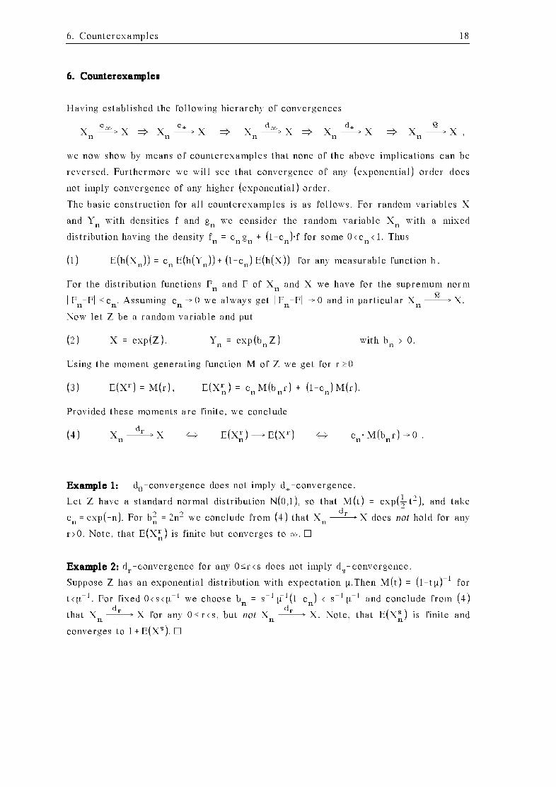
6. Counterexamplee

Having established the following hierarchy of convergences

d+ E X * X * x n % x * X,-X * X , - X ,

we now show by means of counterexamples that none of the above implications can be

reversed. Furthermore we will see that convergence of any (exponential) order does

not imply convergence of any higher (exponential) order.

The basic construction for a l l counterexamples is as follows. For random variables X

and Y, with densities f and gn we consider the random variable X, with a mixed

distribution having the density fn = cngn + (I-C,)-f for some 0 < C, < 1. Thus

(1 E(~(x , ) ) = C, E(~(Y,) ) + (I-C,) E ( ~ ( x ) ) for any measurable function h .

For the distribution functions F, and F of X, and X we have for the supremum norm E

IF,-F1 g C,. Assuming C, + 0 we always get IIF,-FI + 0 and in particular X, - X.

Now let Z be a random variable and put

(2) X = e x p ( z ) , Y, = exp ( b , ~ ) with bn > 0.

Using the moment generating function M of Z we get for r 2 0

Provided these moments a r e finite, we conclude

(4 d

X, AX H E(x:) - E ( x ~ ) H M(b,r) + 0 .

Example 1: d,-convergence does not imply d+-convergence.

Let Z have a standard normal distribution ~ ( 0 , 1 ) , so that ~ ( t ) = exp(&t2) , and Lake d

C, = esp(-n) . For b i = 2n2 we conclude from (4) that X, 2 X does not hold for any

r>O. Note, that E ( x ~ ) is finite but converges to m.

Example 2: dr-convergence for any Ogr < s does not imply ds-convergence.

Suppose Z has an exponential distribution with expectation p.Then ~ ( t ) = (I- tp)- l for

t < p-I. For fixed O < s < p-l we choose bn = s-l pT1(l-C,) < s-' p-I and conclude from (4) d r d r that X, - X for any 0 g r < s , but not X, - X. Note, that E ( x ~ ) is finite and

converges to 1 + E ( x S ) .

6. Counterexamples 19

Example 3: dm-convergence does not imply e+-convergence. E

Taking Z n = log Xn in example 1, we get Zn - Z but not Zn Z for any r > 0

by Lemma 2(v). Furthermore from ( I ) with h(x) = ( 1 0 ~ x ) ~ one obtains E ( z r ) + E ( z r ) n

dm e+ for any r >O. Thus we have Z n - Z but not Z n - Z , although the M G F of Z n

and Z a re finite on IR.

Example 4: er-convergence for any Ogr < s does not imply es-convergence. er Taking Z n = log Xn in example 2, we get by Lemma 2(v) Zn - Z for any 0 g r < s ,

es but not Zn - Z . Note again, that E(exp(s z,)) = E ( x ~ ) is finite and converges to

1+E(exp(s z)) = 1 + E ( x S ) .

The first two examples involve only positive random variables Xn,X, because absolute

moments for these a r e simple to calculate . However other examples a r e easily given,

like the following with a standard normal limit.

Example 5: Convergence of any order 0 g r < 2 to N(0, l) does not imply d2-convergence.

Suppose E(x) = N(o,I) , E(Y,) = N(0,n) and let Xn have a mixed distribution as above d r d2 with c n = 6 ' . Then Xn- X holds for any Ogr < 2, but Xn - X does not hold,

since E(x:) - 2 and Var (X:) - 2.

The last example is of particular interest in statistics, since convergence of a random

variable Xn, e.g. a scaled parameter estimate with E(x , )=O, to a normal limit N(0,02)

a r e often encountered. If we only have convergence in distribution together with

E(x~)-0, but not of convergence of order 2. we can only conclude l i g inf V a r ( x n )

2 o2 Ce.g. Billingsley (1968), Thm.5.31. Hence the "asymptotic" variance o2 of the

normal limit may be considerably smaller than the actual variance of Xn, unless, of

Course, we have convergence of order 2 (like e.g. in the central limit theorem above).

7. Statistical Applications 2 0

7. Statietical Applicatione

To illustrate the concepts and methods above, we now strengthen some results on

asymptotic normality used in statistics to dr-convergence. Further examples of dr-

convergence in connection with bootstrap methods may be found in Bickel & Freedman

(1981) and Freedman (1981).

Traneformation of Binomial Ratee

Let X be b in~mial (n ,~) -d is t r ibuted , and let % = $ X be the observed rate . In some

applications one is interested in the transformed ra te G(%) for a suitable transformation

G:(o , I ) - IR, e.g. the probit- or logit-transformation. Since ~ ( x ) is not defined for iy

X = 0 , X = 1 we use a modified ra te X which coincides with % except for the values 0 , l iy 1 where X takes the values cn-Y, 1-cn-Y for some constants O < c < l , y 2 1 , e.g. C = , y = 1

as Berkson (1955) suggested. iy iy

The difference beetween % and X is negligable as n+ co, since &(%-X) - em 0 by iy

Lemma 2(v). Hence X has the same asymptotic distribution as 2 (see 4 . Example 1)

iy

(1 & ( x - ~ ) - N(O, pq) as n-co and q = 1-p.

Furthermore one can show that

Application of 5. Example 2 gives the following limit result for the transformed ra te ,

provided the transformation G satisfies condition 5(8)

(3) dm h [G(?) - G(P)] - N ( o , o ~ ) as n-co ,

with o2 = pq[G'(p)]2. Note, that 5(9) follows from (2).

7. Statistical Applications 2 1

Log-Odde-Ratio for Poieeon Variablem

Let X l l , X12, X21, X22 be independent random variables having Poisson distributions

with Xij:=~(xij) > 0. Regarding the Xij as a 2x2-contingency table

one is (among other things) interested in the log-odds-ratio of the observed table

U = log X„ + log X„ - log X„ - log X„ .

To derive a limit result for U we first consider log X for a single Poisson random

variable X with E(X) = X. To avoid infinite values of log X we replace X by a random iy iy

variable X which coincides with X except for the value 0 where X takes a fixed value iy

O < C < 1, e.g. C = + . For X + m the difference beetween X and X is negligible since e, iy

X-"~(X - 2) - 0 by Lemma 2(v). Hence X has the same asymptotic distribution as

X (see 4. Example 1)

Application of 5. Example 1 gives

(6) d, fi [log 2 - log X ] - N(O,I) as X + m ,

since the condition 5(4) follows from

W e now return to the table (xij) and consider a limit process X+ m, such that hij/X++ '1

converges to a constant cij > 0 , with X++ = A l l + X12 + X21 + X22. Then the aymptotic iy

distribution of the log-odds-ratio follows easily from (6) applied to each Xij:

1 1 1 with y = X;: + X i 2 + X;, + i2

7. Statistical Applications 2 2

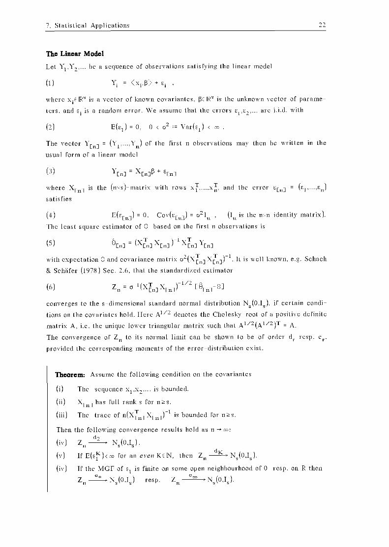
The Linear Model

Let Yl ,Y2,... be a sequence of observations satisfying the linear model

where xiC IRS is a vector of known covariantes, ßC IRS is the unknown vector of parame-

te rs , and zi is a random er ror . W e assume that the errors E ~ , E ~ , . . . a r e i.i.d. with

The vector YCnl = (Y l,...,Yn) of the first n observations may then be written in the

usual form of a linear model

(3) ' C ~ I = '[nlß + ' C ~ I

where XCn1 is the (nxs)-matrix with rows x . . . x and the error ECnl =

satisfies

(4 ) = 0 , C O ~ ( E [ ~ ~ ) = 021n , (In is the nxn identity matrix).

The least square estimator of 9 based on the first n observations is

T with expectation 9 and covariance matrix o2(xCn1 x:~])-~. It is well known. e . g Schach

& Schäfer (1978) Sec. 2.6, that the standardized estimator

coilverges to the s-dimensional standard normal distribution Ns(O,Is), if cer tain condi-

tions on the covariates hold. He re A ~ / ~ denotes the Cholesky-root of a positive definite

matrix A , i.e. the unique lower triangular matrix such that = A.

The convergence of Zn to its normal limit can be shown to be of order dr resp. e r ,

provided the corresponding moments of the error-distribution exist.

r Theorem: As sume the following condition on the covariantes

(i) The sequencexl,x2,...isbounded .

(ii) XCnl has full rank s for n z s.

(iii) The t race of n(XFnl XInl)-l is bounded for n z s

I Then the following convergence results hold as n + m:

(iv) If the MGF of is finite on some Open neighbourhood of 0 resp. on IR then em N ~ ( o , I ~ ) resp. zn - N ~ ( O , I ~ ) .

7. Statistical Applications

Remark 1: If XCnl has full rang for some n.>s, then condition (ii) holds after rearranging

the first n observations.

Remark 2: Condition (iii) follows from the stronger "standard" assumption

(iii)" T n-lxCn1 XCnl - V positive definite, as n + m.

Remark 3: To prove (iv), the condition (i) may be weakened to the following consequence

of (iii)":

(i)" n - l / 2 IIxnl - 0 as n + m .

Proof (~heorem)

ad (iv): By Cramkr-Wold's device it suffices to show for any t~ IR, t*O

(vii) d2 Un := <t,Zn> - ~ ( 0 , lit1i2) .

Without loss of generality, we may assume Iltl = 1. From the representation

T T Zn = '-' ' C ~ I ' C ~ I with C, = (xFn1 XCnl)-1/2

we get

2 (viii) Un = 0-I < a n , ~ C n l > = ani 0 - l ~ ~ with an = XCnlCnt, llanl = 1 1

W e first show for the maximum-norm I - I m a x

(ix 16 Ianlmax is bounded.

This follows from

(X Jn IIanlmax s 2 . IIXCnlllmax~ IJn CnImaX. Iltllmax

together with (i) and (iii) in view of

(xi) AL^^ d t r a c e ( ~ ~ ~ ) for any sxs matrix A.

E Now Unhas expectation 0 , variance 1, and Un- N(0, l) follows from the central

limit theorem, since Lindeberg's condition may be derived from Ianlmax- 0 . And (vi)

follows, since Un is standardized.

ad (v)(vi): The proofs a r e similar to (iii), using Cramkr-Wold's device and the corolla-

ries to the central limit theorems for d- and e-convergence above, which apply in view

of (viii)(ix).

Proof (Remark 3) Condition (i)" implies IXCnllmax- 0 and using ( X ) we get instead of (ix) only

Ianlmax- 0 , which was sufficient to derive (iv) above.

7. Statistical Applications 2 4

Eetimation of Quantilee and the Median

Sen (1959) has shown that the (suitably scaled) distribution of sample quantiles (e.g. the

median) converges to its normal limit of order dr , for any rc IN, as the sample size tends

to infinity, provided of course the underlying sample distribution has certain properties.

W e a re now going to prove this result under slightly different assumptions, using the

asymptotic moments of be ta distributions given in Sen (1959), Sec. 2. and the above

properties of dr-convergence.

Let X1, ..., X, be i.i.d. random variables with a distribution concentrated on some Open

intervall IclR. W e assume that the distribution function F of X1 has a continuous

densitity f = F'>O on I. Then for any O < p < l , the p-th quantile of F is defined by 1 €Ip:= F - ' ( ~ ) C I. Of course p gives the median of F. The estimate of 9 should be the

P

corresponding quantile of the empirical distribution function F, of X I , ..., X, given by

F,(x) = #{ilxign}/n. However F, being a step function has no unique inverse F;' and

the quantile is usually defined as 6p=~;1(p) with some definite choice of inverse like

the le f t resp. right-continuous inverse of a distribution function G given by

(1 G - ( ~ ) = in f ix I p g ~ ( x ) } (left-continuous inverse) resp.

(2) (?(P) = s u p { x I ~ ( x ) g p } (right -continuous inverse)

To be explizit , we Lake Gp = Results for the other estimate may be derived

from those of in view of = - G;(I-~) , where G, is the empirical distribution

function of the variables -Xl,....,-X,. First we derive the limit result for the uniform

distribution on (0 , l ) and generalize to arbitrary continuous distributions using the

8-method.

Theorem 1 (uniform caee): If F is the uniform distribution on I = (0 , I ) then as n + m:

d, (i) ~ [ F ; ( P ) - P ] - ~ ( 0 , ~ ~ ) with q = 1-p.

(ii) E [ F ~ ( ~ ) - ~ ] - p - S , provided n > s / p , S C IN .

(iii) E[ ( I -F ; (~) ) -~] - q - S , provided n > s/q, S C IN .

Remark: The conditions on n in (ii)(iii) garantee the existence of the inverse moments.

7. Statistical Applications 2 5

Proof: 6, = has a Beta(an,bn)-distribution with an+bn= n + l , where an is the

smallest integer 2 np resp. bn is the greatest integer < l+nq. From Sen (1959), (2.11),

(with an,bn interchanged) we get for any sc IN

E { Z y - E { N ( O , ~ ~ ) ~ } , where Zn = 1 h [ 6 ~ - ~ I , pn = E{fin} = an/ (n+l ) .

E d , This implies Z n - N(0,pq) [Billingsley (1979) Thm.30.21, and hence z,-N(o,~~).

Adding &(pn-p) -0 and using 2(3), 2(6) gives (i). Now (ii) follows from

E{6iS} = B(an-s, bn)/B(an.bn) = n(') / (a n -I)( ' ) ,

where B(-,-) is the beta funtion, k( r ) = k(k-1) ...( k- r+ l ) is the descending factorial, and

s < npian . Finally (iii) follows similarly, since 1-en has a Beta(bn,an) distribution. 7

Theorem 2 (~ene ra l ~ a e e )

Let F have a continuous density f = F' > 0 on its support I and assume for some cx20

(i) F ( X ) ~ Cl-F(x)lW f(x)-' is bounded for xc I.

Then for any rc IN and n - co with n > 2 cx-r-max(p-l ,q- l) , q = 1-p:

d r (ii) &[6p-@p]- N(0,02) with

(iii) 02 = ( p q ) / f ( ~ ~ ) ~ .

Remark 1: (i) is a condition on the tails of the distribution and is equivalent to condition

5(8) for G=F- ' . Sen (1958) uses another condition, namely the existence of the 8-th

moment of F for some 8>O, to derive (ii), using slighly different conditions on F.

Remark 2: The condition on n garantees that the r- th moment of the left-hand side in

(ii) exists.

Proof: The variables Yi = F ( x i ) a r e i.i.d. with a uniform distribution on (0, l ) . Since F

has an inverse F : (0 , l ) - I we get Xi = F- ' (Y~). For the empirical distribution

function Fn resp. H n of Xi resp. Yi we have F; = F - l O H ; . By Thm. l ( i ) we have

Ih[H;(p)-p] 5 N(O,pq), and application of the S m e t h o d (see 5. Example 2 with

G = F-l) will give (ii)(iii) provided condition 5(9) holds for t = 2 r, i.e. - 2 ~ r and

[I- H;(p a r e uniformly integrable. And this follows from Thm. 1 (ii-iii) for

n > 2 cx-r. max{p-l,q- '}. 7

References 2 6

Referencee

Berkson, ~ . (1953) : A Statistically Precise and relatively simple Methods of Estimating

the Bioassay with Quanta1 Response, Based on the Logistic Function.

Journal of American Statistical Association,44, 565-599.

Bickel, P.J., Freedman, ~ . ~ . ( 1 9 8 1 ) : Some Asymptotic Theory for the Bootstrap.

The Annals of Statistics, 9, 1196-1217.

Billingsley, ~ . ( 1 9 6 8 ) : Convergence of Probability Measures. Wiley, New York.

Billingsley, ~ . ( 1 9 7 9 ) : Probability and Measure. Wiley, New York.

Bishop, Y.M.M., Fienberg, S.E., Holland, ~ . ~ . ( 1 9 7 5 ) . Discrete Multvariate Analysis:

Theory and Practice. Cambridge ( ~ a s s . ) , MIT-Press.

Dieudonne, ~ . (1960) : Foundations of Modern Analysis. Academic Press, New York.

Freedman, ~ . ~ . ( 1 9 8 1 ) : Bootstrapping Regressions Models.

The Annals of Statistics, 9, 1218-1228,.

Johnson, N.L., Kotz, ~ . (1970-72) : Distribution in Statistics.

Vol. 1-4, New York, Wiley.

Schach, S., Schäfer, Th. (1978). Regressions- und Varianzanalyse. Berlin, Springer.

Sen, ~ . ~ . ( 1 9 5 9 ) : On the Moments of the Sample Quantiles.

Calcutta Statistical Association Bulletin, 9, 1-19.

Adress of author: Prof. Dr . Gerhard Osius

Universität Bremen, Fachbereich 3 ( ~ a t h e m a t i k A n f o r m a t i k )

28334 Bremen, Postfach 33 04 40

Germany

e-mail: osius@math.uni-bremen.de

Date: 21-Mar-1989 (printed edition) 8-Jan-2001 ( P D F - ~ i l e , with minor corrections)

Universität Bremen Mathematik-ArbeitspapiereStand November 2000 ISSN 0173 - 685 X

Vertrieb der Hefte 4, 14, 23, 26 durch Universitätsbuchhandlung, Bibliothekstr. 3, D-28359 Bre-men. Vertrieb der übrigen Hefte (soweit nicht vergriffen) durch die Autoren oder FB 3 Mathema-tik/Informatik Universität Bremen, Postfach 330440, D-28334 Bremen.

1. Ulrich Krause (1976): Strukturen in unendlichdimensionalen konvexen Mengen, 74 S.

2. Fritz Colonius, Diederich Hinrichsen (1976): Optimal control of heriditary differential systems.Part I, 66 S.

3. Günter Matthiessen (1976): Theorie der heterogenen Algebren, 88 S.

4. H. Wolfgang Fischer, Jens Gamst, Klaus Horneffer (1976): Skript zur Analysis, Band 1 (11.Auflage 2000), 286 S.

5. Wolfgang Schröder (1977): Operator-algebraische Ergodentheorie für Quantensysteme, 59S.

6. Rolf Röhrig, Michael Unterstein (1977): Analyse multivariabler Systeme mit Hilfe komplexerMatrixfunktionen, 216 S.

7. Horst Herrlich, Hans-Eberhard Porst, Rudolf-Eberhard Hoffmann, Manfred Bernd Wisch-newsky (1976): Nordwestdeutsches Kategorienseminar, 193 S.

8. Fritz Colonius, Diederich Hinrichsen (1977): Optimal Control of Hereditary Differential Sy-stems. Part II: Differential State Space Description, 36 S.

9. Ludwig Arnold (1977): Differentialgleichungen und Regelungstheorie, 185 S.

10. Rudolf Lorenz (1977): Iterative Verfahren zur Lösung großer, dünnbesetzter symmetrischerEigenwertprobleme, 104 S.

11. Konrad Behnen, Hans-Peter Kinder, Gerhard Osius, Rüdiger Schäfer, Jürgen Timm (1977):Dose-Response-Analysis, 206 S.

12. Hans-Friedrich Münzner, Dieter Prätzel-Wolters (1978): Minimalbasen polynomialer Moduln,Strukturindizes und BRUNOVSKY-Transformationen, 53 S.

13. Konrad Behnen (1978): Vorzeichen-Rangtests mit Nullen und Bindungen, 53 S.

14. H. Wolfgang Fischer, Jens Gamst, Klaus Horneffer, Eberhard Oeljeklaus (1978): Skript zurLinearen Algebra, Band 1 (13. Auflage 2000), 249 S.

15. Günter Ludyk (1978): Abtastregelung zeitvarianter Einfach- und Mehrfachsysteme, 54 S.

16. Momme Johs Thomsen (1977): Zur Theorie der Fastalgebren, 146 S.

17. Klaus Horneffer, Horst Diehl (1978): Modellrechnungen zur anaeroben Reduktionskinetik desCytochroms P-450, 34 S.

18. Horst Herrlich, Rudolf-Eberhard Hoffmann, Hans-Eberhard Porst, Manfred Bernd Wischnews-ky (1979): Structure of Topological Categories, 252 S.

19. Hans-Friedrich Münzner, Dieter Prätzel-Wolters (1979): Geometric and moduletheoretic ap-proach to linear systems. Part I: Basic categories and functors, 28 S.

20. Hans-Friedrich Münzner, Dieter Prätzel-Wolters (1979): Geometric and moduletheoretic ap-proach to linear systems. Part II: Moduletheoretic characterization and reachability, 28 S.

21. Eckart Beutler, Hans Kaiser, Günter Matthiessen, Jürgen Timm (1979): Biduale Algebren,165 S.

22. Horst Diehl, Detlef Harbach, Jürgen Timm (1980): Planung und Auswertung von Atomabsorp-tions-Spektrometrie-Untersuchungen mit der Additionsmethode, 44 S.

23. H. Wolfgang Fischer, Jens Gamst, Klaus Horneffer (1981): Skript zur Analysis, Band 2 (6.Auflage 1996), 299 S.

24. Horst Herrlich (1981): Categorical Topology 1971-1981, 105 S.

25. Horst Herrlich, Rudolf-Eberhard Hoffmann, Hans-Eberhard Porst, Manfred Bernd Wischnews-ky (1981): Special Topics in Topology and Category Theory, 108 S.

26. H. Wolfgang Fischer, Jens Gamst, Klaus Horneffer (1984): Skript zur Linearen Algebra, Band2 (7. Auflage 1999), 257 S.

27. Rudolf-Eberhard Hoffmann (1982): Continuous Lattices and Related Topics, 314 S.

28. Horst Herrlich, Rudolf-Eberhard Hoffmann, Hans-Eberhard Porst (1987): Workshop on Cate-gory Theory, 169 S.

29. Harald Boehme (1987): Zur Berufspraxis des Diplommathematikers, 16 S.

30. Jürgen Timm (1986): Mathematische Modelle der Dosis-Wirkungsanalyse bei den experimen-tellen Untersuchungen der Arbeitsgruppe zur karzinogenen Belastung des Menschen durchLuftverunreinigung, 65 S.

31. Dieter Denneberg (1988): Mathematik für Wirtschaftswissenschaftler. I. Lineare Algebra, 97S.

32. Peter E. Crouch, Diederich Hinrichsen, Anthony J. Pritchard, Dietmar Salamon (1988, pre-vious edition University of Warwick 1981): Introduction to Mathematical Systems Theory, 244S.

33. Gerhard Osius (1989): Some Results on Convergence of Moments and Convergence in Dis-tribution with Applications in Statistics, 27 S.

34. Dieter Denneberg (1989): Verzerrte Wahrscheinlichkeiten in der Versicherungsmathematik,Quantilsabhängige Prämienprinzipien, 24 S.

35. Eberhard Oeljeklaus (1989): Birational splitting of homogeneous Albanese bundles, 30 S.

36. Gerhard Osius, Dieter Rojek (1989): Normal Goodness-of-Fit Tests for Parametric MultinomialModels with Large Degrees of Freedom, 38 S.

37. Dieter Denneberg (1990): Mathematik zur Wirtschaftswissenschaft. II. Analysis, 59 S.

38. Ulrich Krause, Cornelia Zahlten (1990): Arithmetik in Krull monoids and the cross number ofdivisor class groups, 29 S.

39. Dieter Denneberg (1990): Subadditive Measure and Integral, 39 S.

40. Ulrich Krause, Peter Ranft (1991): A limit set trichotomy for monotone nonlinear dynamicalsystems, 31 S.

41. Angelika van der Linde (1992): Statistical analyses with splines: are they well defined? 22 S.

42. Dieter Denneberg (1992): Lectures on non-additive measure and integral (new edition: Non-additive measure and integral. TDLB 27, Kluwer Academic, Dordrecht (1994)), 114 S.

43. Gerhard Osius (1993): Separating Agreement from Association in Log-linear Models forSquare Contingency Tables With Applications, 23 S.

44. Hans-Peter Kinder, Friedrich Liese (1995): Bremen-Rostock Statistik Seminar, 5. - 7. März1992, 110 S.

45. Dieter Denneberg (1995): Extension of a measurable space and linear representation of theChoquet Integral, 30 S.

46. Dieter Denneberg, Michael Grabisch (1996): Shapley value and interaction index, 20 S.

47. Angelika Bunse-Gerstner, Heike Faßbender (1996): A Jacobi-like method for solving alge-braic Riccati equations on parallel computers, 24 S.

48. Hans-Eberhard Porst editor (1997): Categorical methods in algebra and topology - a collec-tion of papers in honour of Horst Herrlich, 498 S.

49. Angelika van der Linde, Gerhard Osius (1997): Estimation of nonparametric risk functions Inmatched case-control studies, 28 S.

50. Angelika van der Linde (1997): Estimating the smoothing parameter in generalized spline-based regression, 46 S.

51. Ursula Müller, Gerhard Osius (1998): Asymptotic normality of goodness-of-fit statistics forsparse Poisson data, 15 S.

52. Ursula Müller (1999): Nonparametric regression for threshold data, 18 S.

53. Gerhard Osius (2000): The association between two random elements – A complete charac-terization in terms of odds ratios, 32 S.