some recent developments in numerical methods...

COMPUTER METHODS IN APPLIED MECHANICS AND ENGINEERING 51(1985) 467-493 NORTH-HOLLAND

SOME RECENT DEVELOPMENTS IN NUMERICAL METHODS FOR T~NSO~C FLOWS

Anthony JAMESON Department of Mechanical and Aerospace Engineering, Princeton University, U.S.A.

Wolfgang SCHMIDT Domier Gm bH, D- 7990 ~~ed~~hshafen~ Fed. Rep. Germany

Received 24 December 1984

1. Intr~uction

The objective of this paper is to discuss a satisfactory numerical method for the calculation of steady solutions of the Euler equations for inviscid compressible gas flows and extensions to the treatment of the Navier-Stokes equations and time-dependent flows. The intended application is the prediction of the aerodynamic properties of airplanes flying at transonic speeds. This will ultimately call for solutions of the viscous equations. The Reynolds numbers prevailing in full-scale flight are typically very large, with the result that the boundary layers become turbulent, forcing recourse to statistical averaging and the introduction of turbulence models. We may regard the solution of the Euler equations as a way station on the route to this longer-term objective.

Some of the principal difficulties of the problem are: (1) The equations of gas dynamics are nonlinear. (2) Solutions in the transonic range will ordinarily be discontinuous. Thus we may expect to

find shock waves. The solutions will also generally contain contact surfaces in the form of vortex sheets (shed both by wings in three-dimensional flow, and also by profiles in two- dimensional flow in the event that shock waves of differing strength produce different amounts of entropy on the upper and lower surfaces).

(3) There are regions of the flow in the neighborhood, for example, of stagnation points, the wing trailing edge or the wing tip, where the derivatives may become very large or even unbounded, leading to large discretization errors.

(4) The equations are to be solved in an unbounded domain. (5) We are generally interested in calculating flows over bodies of extreme geometric

complexity (including cases where the domain is multiply connected). In order to find one’s way through this thicket of difficulties and pitfalls, Peter Lax has

suggested the need for ‘design principles’ to guide the construction of a numerical scheme appropriate to the problem, A steady solution is obtained as the asymptotic state of a time- dependent problem. Since the unsteady problem is used only as a vehicle for reaching the steady state, alternative iterative schemes might be contemplated. An example is the least squares method, which has reached a high level of sophistication at the hands of Glowinski

00457825/85/$3.30 @ 1985, Elsevier Science Publishers B.V. worth-Holland)

468 A. Jameson, W. Schmidt, Recent developments in numerical methods for transom? f7ows

and his co-workers. We believe, however, that the time-marching formulation is worth considering for some of the following reasons:

(1) Its simplicity (with consequent reduction of the risk of programming error). (2) It offers the possibility of providing a dual-purpose computer program for both steady

and unsteady problems. (3) Where there is a possibility of a non-unique steady state or perhaps a non-physical

solution, containing, for example, a discontinuous expansion, one may rely on the modelling of a true physical process to make an appropriate selection.

(4) Algorithms can rather easily be devised which take maximum advantage of vector computers.

None of these virtues could be considered decisive if the convergence of the time-marching schemes to a steady state were excessively slow in comparison with competing methods. We hope to show, however, that the time-marching method can be modified in such a way that this need not be the case.

Within the framework of the time-marching formulation the design principles which have guided this work are:

(1) The conservation laws of gas dynamics will be satisfied in discrete conse~ation form by the numerical approximation. (We may then rely on the theorem of Lax and Wendroff that the correct shock jump and contact discontinuity conditions will be satisfied by the solution if it converges in the limit of decreasing mesh width.)

(2) Unphysical solutions are to be excluded by the introduction of appropriate dissipative terms in the discrete approximation.

(3) The final steady state should be independent of the time-marching procedure. This requirement does exclude the use of a number of popular difference schemes, including schemes with fractional steps, and the Lax-Wendroff and MacCormack schemes.

(4) If a quantity is known to be invariant in the true solution, it should also be invariant in the numerical solution. In particular, the total enthalpy should be constant in the steady-state solution.

(5) Uniform flow should be an exact solution of the difference equations on an arbitrary mesh.

In order to meet requirement (3) we believe that it is helpful to separate the space discretization procedure entirely from the time-marching procedure by applying first a semi-discretization. This has the advantage of allowing the problems of spatial discretization error, artificial dissipation and shock modelling to be studied independently of the problems of time-marching stability and convergence acceleration.

The main measures for accelerating the convergence to steady state which have been applied in this work are:

(1) Modification of the differential equations for faster convergence to a steady state. (2) The use of a hybrid multistage time-stepping scheme with distinct and separately

optimized treatment of the hyperbolic and parabolic terms. (3) The use of residual averaging to permit a larger time step without violating stability

restrictions. (4) Parallel time stepping on multiple grids. The use of all these measures in conjunction has made it possible to obtain satisfactory

solutions of the Euler equations for two-dimensional flows in 25-50 steps on fine meshes. Since we first proposed the use of multistage time-stepping schemes for solving the Euler

A. Jameson, W. Schmidt, Recent developments in numerical methods for tiansonic flows 469

equations [l], numerous modifications of both the time-stepping and space-discretization schemes have been introduced, and the treatment of the boundary conditions has also been altered. In this paper we summarize the method as it now stands. Modifications of the Euler equations for faster convergence to a steady state are reviewed in the next section. Section 3 discusses the spatial discretization scheme which is derived from the integral form of the conservation laws. Section 4 discusses a relatively simple form of adaptive dissipation which leads to reasonably satisfactory modelling for shock waves in steady flows. Section 5 discusses modifications to the scheme to improve shock resolution. These rely on more complicated constructions of artificial dissipation based on the concept of diminishing total variation for scalar conservation laws, following the ideas of Lax, Harten, van Leer and Osher [23]. In the light of this discussion it can be seen that the adaptive dissipation can be designed to yield a scheme which locally behaves like a TVD scheme in the neighborhood of a shock wave. The optimal construction, however, requires a decomposition into characteristic fields along the lines proposed by Roe [45]. Section 6 presents a class of hybrid multistage time-stepping schemes, while Sections 7 and 9 review the residual-averaging and multiple-grid schemes. Section 8 gives a short summary on the treatment of boundary conditions. Section 10 presents results to show the influence of variations of parameters and mesh effects. First results for a triangular mesh are also included. Comparisons with potential flow results on shockless configurations and an analysis of total pressure losses for flows with shocks validate the accuracy of the method. First results for turbulent Navier-Stokes solutions using the same scheme are also presented.

2. Modified Euler equations to improve convergence to steady state

The motion of an inviscid compressible gas is governed by the Euler equations. Let p, p, u, u, E, H and c denote the pressure, density, Cartesian velocity components, total energy, total enthalpy and speed of sound. For a perfect gas

E= ’ (Y - VP

+ $(u’+ v2) ) H=E+plp, c2 = YPIP 7 (24

where y is the ratio of specific heats. Using Cartesian space coordinates x and y, the Euler equations for a two-dimensional time-dependent flow are

where t is the time coordinate and

P

PU

PV

PE

PV

PVU

Pv2+P

PVH

(2.2)

(2.3)

These equations are to be solved for a steady state awlat = 0.

470 A. Jameson, W. Schmidt, Recent developments in numerical methods for transonic flows

Aside from trying to construct the most efficient possible numerical method, it is natural to consider the possibility of modifying the Euler equations to improve the rate of convergence to a steady state. Three main approaches have been tried in this work.

The first is to use locally varying time steps such that the difference scheme operates everywhere in the flow field close to its stability limit. This is equivalent to solving

(2.4

where (Y is a variable scaling factor. This method ensures that disturbances will be propagated to the outer boundary in a fixed number of steps, proportional to the number of mesh intervals between the body and the outer boundary.

The second approach is based on the observation that if the enthalpy has a constant value H, in the far field, it is constant everywhere in a steady flow, as can be seen by comparing the equations for conservation of mass and energy. If we set H = H, everywhere in the flow field throughout the evolution, then the pressure can be calculated from the equation

y-1 p=- .

Y > (2.5)

This eliminates the need to integrate the energy equation. The resulting three equation model still constitutes a hyperbolic system, which approaches the same steady state as the original system. The use of this model has been advocated by Veuillot and Viviand [6] and Schmidt and Rizzi [7].

The third approach is to retain the energy equation, and to add forcing terms proportional to the difference between H and H, [l]. In a subsonic irrotational flow one can introduce a velocity potential $J and set

The Euler equations then reduce to the unsteady potential flow equation

Cjn + 2U& + 2v& = (c2 - u2>&X - 2l&X, + (c2 - v2)& * (2.6)

This is simply the equation for undamped wave motion in a moving coordinate frame. Damping could be introduced by adding a term a+, to this equation. Such a term cannot directly be added to the Euler equations. However, the Bernoulli equation for unsteady potential flow is

&+H=H,,

Thus one can simulate the addition of a term CUE, to (2.6) by adding terms proportional to H - H, to the Euler equations. Provided that the space discretization scheme is constructed in such a way that H = H, is consistent with the steady-state solution of the difference equations, these terms do not alter the final steady state. Numerical experiments have confirmed that

A. Jameson, W. Schmidt, Recent developments in numerical methods for transonic flows 471

they do assist convergence. The terms added to the mass and momentum equations are cyp(H - Ha), apu(H - H,), while that added to the energy equation is aP(H - H,). In calculations using multiple grids an effective strategy is to include these terms only on the fine grid, and to increase the parameter (Y.

3. Finite volume formulation

The space-discretization scheme is developed by writing the Euler equations in integral form

~I~~wdS+I_(fdy-gdx)=O (3.1)

for a domain S with boundary aS. The computational domain is divided into quadrilateral cells denoted by the subscripts i, j. Assuming that the dependent variables are known at the center of each cell, a system of ordinary differential equations is obtained by applying equation (3.1) separately to each cell. These have the form

%(sjWi,j)+ Qi,j = 0 9 (3.2)

where Sivj is the cell area, and Qi,j is the net flux out of the cell. This may be evaluated as

(3.3)

where fk and gk denote values of the flux vectors f and g on the kth edge, Axk and Ay, are the increments of x and y along the edge with appropriate signs, and the sum is over the four sides of the cell. The flux vectors are evaluated by taking the average of the values in the cells on either side of each edge. For example

fi=i(fi+l,j+fi,j), (3.4)

where fi,j denotes f(wi,j)e Alternatively one may evaluate first the flux velocity

Q/c = AJ’k(PU)k -h(Pv)k

Pk

on each edge. Then the flux for the x momentum component, for example, is

4

2 {Qk(&k + AYkPd .

k=l (3.5)

Schemes constructed in this manner reduce to central difference schemes on Cartesian meshes,


and are second-order accurate if the mesh is sufficiently smooth. They also satisfy the design principle (5) that uniform flow should be an exact solution of the difference equations. Provided that they are augmented by appropriate dissipative terms, they have been found to give quire accurate results, and they can easily be extended to three-dimensional flows [8, 9, 10, 111.

4. Adaptive dissipation

The finite volume scheme (3.2) is not dissipative, allowing undamped oscillations with alternate sign at odd and even mesh points. In order to eliminate spurious oscillations, which will be triggered by discontinuities in the solution, one can follow either of two strategies. The first is to begin with a non-dissipative scheme such as (3.2), or a fourth-order scheme, and to add just enough dissipation where it is needed to control the tendency to produce spurious oscillations. The second approach, which can be traced to the work of Boris, Book and Zalesak [12,13], is to begin by adding enough dissipation everywhere to guarantee the absence of unwanted oscillations. This leads to a first-order accurate scheme which excessively smears dis~ontinuities. A correction is then added to cancel the first-order error, but the correction is limited to prevent the introduction of overshoots near discontinuities. This idea is the basis of an ingenious method recently proposed by Harten [14] for the construction of schemes which promise to give sharp resolution of shock waves. In this section we describe an adaptive scheme for adding dissipation which has proved effective in practice, and in the next section, we shall consider the more complex high-resolution schemes. The idea of the adaptive scheme is to add third-order dissipative terms throughout the domain to provide a base level of dissipation su~~ient to prevent nonlinear instability, but not sufficient to prevent oscillations in the neighborhood of shock waves. In order to capture shock waves additional first-order dissipative terms are added locally by a sensor designed to detect discontinuities.

With the addition of dissipative terms -Di,j, the semi-discrete equations (3.2) take the form

(4.1)

To prevent conservation form the dissipative terms are generated by dissipative fluxes. The dissipation for the density equation, for example, is

where the dissipative flux di+z/2,i is defined by

d i+l,z,j = &~~2!1/2,jRi+l/2,j(Pi,j -pi-~,j)- &~~4?1/2,jRi+1/2,j(Pi+Z,j - 3Pi+l.j + 3Pt.j -Pi-l,j) 1

(4.3)

Here E$$‘~,~, i and E$$‘~,~,~ are adaptive coefficients, and R i+l/z,j is a coefficient chosen to give the dissipative terms the proper scale. An appropriate scaling factor is

A. Jameson, W, Schmidt, Recent developments in numerical methods for transonic flows 473

where A is the spectral radius of the Jacobian matrix

for the flux across the cell face. This can be estimated as

h=luAy-vAx~+dAx2+Ay2, (4.5)

where c is the speed of sound, and Ax and Ay are the displacements of the face in the x and y directions.

If one is using an explicit time-stepping scheme one needs an estimate of the time-step limit. A conservative estimate for a nominal Courant number of unity is

Atzi = S,j

Ai,j + ,Ui,j ’

where Ai,j and pi,j are the average spectral radii of the Jacobian matrices in the i and j directions. It is then convenient to avoid duplicate calculations by taking

(4.4*)

An effective sensor of the presence of a shock wave can be constructed by taking the second difference of the pressure. Define

Set

Then we

I pi+l, j -2pi.j +pi-1,j Vi,j =

pi+l, j I + 2pi,j +pi-1.j ’

Vi+1/2, j = maX(Vi+z, j, Vi+l, j, Vi, j9 Vi-l, j> *

take

E$:)~,~, k = min($, k(2)fii+1,2,j) and ~$?1,2,j = max(0, kc4’ - avi+l,z,j) , F-7)

(4.6)

where k@‘, kC4’ and cy are constants. Typically,

k(2) = 1 7

k(4) = 1 32, ff=2.

In a smooth region of the flow vi,j is proportional to the square of the mesh width, with the result that &c2) r+l/Z. j is also proportional to the square of the mesh width, while &:$‘1/2,j is of order one, and the dissipative fluxes are of third order in comparison with the convective fluxes. In the neighborhood of a shock wave vi,j is of order 1, so that the scheme behaves locally like a first-order scheme. The term aVi+ln,j is subtracted from kf4’ to cut off the fourth differences which would otherwise cause an oscillation in the neighborhood of the shock wave.


The dissipative terms for the momentum and energy equations are constructed in the same way as those for the mass equation, substituting pu, pv or pH for p in equation (4.3). The purpose of using differences of pH rather than pE in the dissipative terms for the energy equation is to produce difference equations which admit the solution H = H, in the steady state. With this choice the energy equation reduces to the mass equation multipled by H,

when the time derivatives vanish.

5. Schemes designed to improve the resolution of shock waves

There is by now a rather extensive theory of difference schemes for the treatment of a scalar conservation law

~+df(u)=0. af ax

This theory stems from the mathematical theory Lax [15]. It is known that the total variation

TV=

(5.1)

of shock waves, as it has been formulated by

of a solution of (5.1) can never increase. Correspondingly total variation

it seems desirable that the discrete

of a solution of a difference approximation to (5.1) should not increase. A semi-discretization will have this property (now generally called total variation diminishing or TVD) if it can be cast in the form

dui - = C~+I~*(4+1~ Ui)- CL-l/*(& - W-1) >

dt (5.2)

where the coefficients c;+~,~ and c;_~,~ are non-negative [16, 171. Since the total variation will increase if an initially monotone profile ceases to be monotone,

TVD schemes preserve monotonicity. The TVD property does not, however, guarantee fulfilment of the entropy condition that the only admissible discontinuous solutions are those for which the characteristics of (5.1) converge on the discontinuities from both sides [15]. Some TVD schemes admit stationary expansion shock waves, for example.

The concept of converting a first-order monotone scheme to a second-order scheme by adding an anti-diffusive flux which is limited to prevent spurious oscillations may already be found in the work of Boris, Book and Zalesak [12,13]. Harten’s advance was to develop a mathematical formulation of the idea which allowed the TVD property to be proved for a


second-order scheme. The concept of flux limiting was independently introduced by van Leer

WI* There are difficulties in extending these ideas to systems of equations, and also to equations

in more than one space dimension. Firstly the total variation of the solution of a system of hyperbolic equations may increase. Secondly it has been shown by Goodman and Leveque that a TVD scheme in two space dimensions is no better than first-order accurate [19]. One might add dissipative terms by applying the same construction to the complete system of equations, using for czi+1/2 the spectral radius of the Jacobian matrix df/du, evaluated for an average value Ui+ l/2 a Numerical experiments indicate that this leads to an excessively dissipative scheme. It can be seen, however, that with the scaling (4.4) the adaptive dissipation proposed in the previous section leads to a scheme which will behave locally like a TVD scheme if the constants are chosen to make sure that the coefficient &!:)1/2,j = 4 in the neighborhood of a shock wave. This will be illustrated in Section 9 for the case of Burgers’ equation and for a transonic airfoil flow. Further details on the construction of TVD schemes can be found in [16,20].

6. Hybrid multistage time-stepping schemes

Multistage schemes for the numerical solution of ordinary differential equations are usually designed to give a high order of accuracy. Since the present objective is simply to obtain a steady state as rapidly as possible, the order of accuracy is not important. This allows the use of schemes selected purely for their properties of stability and damping. For this purpose it pays to distinguish the hyperbolic and parabolic parts stemming respectively from the convective and dissipative terms, and to treat them differently. This leads to a new class of hybrid multistage schemes.

Since the cell area Si,j is independent of time, equation (4.1) can be written as

%+R(w)=O, where R(w) is the residual

Ri.j = $(Qi,j-Di,j).

1. I

(6.1)

(6.2)

Let W be the value of w after n time steps. Dropping the subscripts i,i the general m stage hybrid scheme to advance a time step At can be written as

w(o) = w” 9

wm = w(O) - alAtRco) ,

w(“-‘) = w(‘J) _ a,_lAtR(m-2) 9

W(m) = w(o) _ AtR’“-1’ 7

W n+l _ - w(m) )

(6.3)


where the residual in the (q + 1) st stage is evaluated as

RC4) = ; j$ @,rQ(w”‘) - yqrD(w(‘))} I 0

subject to the consistency constraint that

i pqr = i Yq, = 1 *

FO r=O

(6.4)

A simple procedure is to recalculate the residual at each stage using the most recently updated value of w. Then (6.4) becomes

R(4) = $ (Q(W’4’) - D(w’4’)) . (6.6)

Schemes of this subclass have been analyzed in a book by van der Houwen [21], and more recently in papers by Sonneveld and van Leer [22], and Roe and Pike [23]. They are second-order accurate in time for both linear and nonlinear problems if am-l = t. An efficient 4-stage scheme, which is also fourth-order accurate for linear problems, has the coefficients

c21= 4, a2= 5, cQ=f. (6.7)

A substantial saving in computational effort can be realized by evaluating the dissipative part only once. This leads to a class of schemes in which (6.4) becomes

(6.8)

Schemes in the subclass defined by (6.8) are clearly more efficient than the more conventional schemes defined by (6.6) in which the dissipative terms are repeatedly evaluated.

If the time-stepping scheme is to be used in a multigrid procedure it is important that it should be effective at damping high-frequency modes. One can fairly easily devise 3- and 4-stage schemes in the class defined by (6.8) which meet this requirement. An effective 3-stage scheme is given by the coefficients

(Y~ = 0.6, a2 = 0.6 . (6.9)

Additional flexibility is provided by a class of schemes in which the dissipative terms are evaluated twice. This may be used to make a further improvement in the high-frequency damping properties, or else to extend the stability region along the real axis to allow more margin for the dissipation introduced by an upwind or TVD scheme of the type described in Section 5. In this class of schemes

A. Jameson, W. ~hm~dt, Recent d~eioprne~t~ in n~me~cal meth~ for transonic flows 477

R@’ = $ (Q(w@‘) - D(w’O’)} ,

R(4) = $2(w(q),- /3D(w”‘)_- (1- p)D(w@‘)},

(6.10)

q 2 1 .

Coefficients for corresponding 4- and Sstage schemes providing good stability characteristics were found to be

1 a1 = z7 Lyz=;, 1

a3=z!, P=l, (6.11)

al=;, a2=$, 3 a3 = 8, tY‘$=$, p=1. (6.12)

7. Residual averaging

A simple method of increasing the time step is to replace the residuals by weighted averages of the neighboring residuals [lo]. Consider the general multistage scheme (6.3). In a one- dimensional case one might replace the residual Ri by the average

Ri = &Ri_I f (1 - 2&)Ri + ERi+l (7.1)

at each stage of the scheme. This smooths the residuals and also increases the support of the scheme, thus relaxing the restriction on the time step imposed Lewy condition. If E > $, however, there are Fourier modes such

by the_ Courant-Friedrichs- that Ri = 0 when Ri # 0. TO

avoid this restriction one may perform the averaging implicity by setting

-ERi-l C (1+ 2c)Ri - ERi+l= Ri a (7.2)

For an infinite interval this equation has the explicit solution

Ri = E 2 rqRi+q, 4 OA

where

e=@+-+, r<l.

(7.3)

(7.4)

Thus the effect of the implicit smoothing is to collect information from residuals at all points in the field, with an influence coefficient which decays by factor r at each additional mesh interval from the point of interest.

In the case of a finite interval with periodic conditions equation (7.3) still holds, provided that the values Ri+q outside the interval are defined by periodicity. In the absence of periodicity one can also choose boundary conditions such that (7.3) is a solution of (7.2), with Ri+q = 0 if i + q lies outside the interval. This solution can be realized by setting

478 A. Jameson, W. Schmidt,

I& = R, ,

Recent developments in numerical methods for transonic flows

Ri = Ri - r(Ri - pi-1) for 2SiSn

and then

1 R, =-fi;,,

l+r

Ri = &i - r(&i - Ei+,) for lSi<n-1.

In the two-dimensional case the implicit residual averaging is applied in product form

(1 - &x8:)(1 - Ey8t))R,i = Ri,j )

where 62 and 8: are the second difference operators in the x and y directions, and E, and E, are the corresponding smoothing parameters.

In practice the best rate of convergence is generally obtained by using a value of Courant number A about three times A*, and the smallest possible amount of smoothing to maintain stability. The idea of residual averaging may be compared with Lerat’s implicit scheme [24]. This may be interpreted as a method of smoothing the corrections calculated by a 2-stage scheme. In the general case of an m-stage scheme it is not sufficient to smooth the final corrections after the m th stage. It is possible, however, to devise stable schemes by smoothing the residuals at alternate stages, starting with the first stage if m is odd, and the second stage if m is even.

8. Boundary conditions

At a solid boundary the only contribution to the flux balance (3.3) comes from the pressure. The normal pressure gradient ap/&z at the wall can be estimated from the condition that a(~~)/& = 0, where qn is the normal velocity component. The pressure at the wall is then estimated by extrapolation from the pressure at the adjacent cell centers, using the known value of aplan.

The rate of convergence to a steady state will be impaired if outgoing waves are reflected back into the flow from the outer boundaries. The treatment of the far-field boundary condition is based on the introduction of Riemann invariants for a one-dimensional flow normal to the boundary. Let subscripts ~0 and e denote free-stream values and values extrapolated from the interior cells adjacent to the boundary,. and let qn and c be the velocity component normal to the boundary and the speed of sound. Assuming that the flow is subsonic at infinity, we introduce fixed and extrapolated Riemann invariants

2c, R = qnm--

2ce

Y-l and R,= q,,+-

y-1 (8.1)

corresponding to incoming and outgoing waves. These may be added and subtracted to give

A. Jameson, W. ~~rnidt, Recent deuelopmen~ in numerical rne~~ods for iranso~ic flows 479

9” = $(I?, f %) and c = i(y - l)(R, - $7,) , (8.2)

where 4” and c are the actual normal velocity component and speed of sound to be specified in the far field. At an outflow boundary, the tangential velocity component and entropy are extrapolated from the interior, while at an inflow boundary they are specified as having free-stream values. These four quantities provide a complete definition of the flow in the far field. If the flow is supersonic in the far field, all the flow quantities are specified at an inflow boundary, and they are all extrapolated from the interior at an outflow boundary.

9. Multigrid scheme

While the available theorems in the theory of multigrid methods generally assume ellip- ticity, it seems that it ought to be possible to accelerate the evolution of a hyperbolic system to a steady state by using large time steps on coarse grids, so that disturbances will be more rapidly expelled through the outer boundary. The interpolation of corrections back to the fine grid will introduce errors, however, which cannot be rapidly expelled from the fine grid, and ought to be locally damped if a fast rate of convergence is to be attained. Thus it remains important that the driving scheme should have the property of rapidly damping out high frequency modes.

In a novel multigrid scheme proposed by Ni [25], the flow variables are stored at mesh nodes, and the rates of change of mass, momentum and energy in each mesh cell are estimated from the flux integral appearing in equation (3.1). The corresponding change 6w in the flow variables is then distributed unequally between the nodes at its four corners. The distribution rule is such that the accumulated corrections at each node correspond to the first two terms of a Taylor series in time, like a Lax-Wendro~ scheme. As it stands, this scheme does not damp oscillations between odd and even points. Ni introduces artificial viscosity by adding a further correction proportional to the difference between the value at each corner and the average of the values at the four corners of the cell. Residuals on the coarse grid are formed by taking weighted averages of the corrections at neighboring nodes of the fine grid, and corrections are then assigned to the corners of coarse grid cells by the same distribution rule. When several grid levels are used, the distribution rule is applied once on each grid down to the coarsest grid, and the corrections are then interpolated back to the fine grid. Using 3 or 4 grid levels, Ni obtained a mean rate of convergence of about 0.95, measured by the average reduction of the residuals in a multig~d cycle. The performance of the scheme seems to depend critically on the presence of the added dissipative terms to provide the necessary damping of high- frequency nodes. In Ni’s published version of the scheme these introduce an error of first order.

The flexibility in the formulation of the hybrid multistage schemes allows them to be designed to provide effective damping of high-frequency modes with higher-order dissipative terms. This makes it possible to devise rapidly convergent multigrid schemes without any need to compromise the accuracy through the introduction of excessive levels of dissipation [26].

In order to adapt the multistage scheme for a multig~d algorithm, auxiliary meshes are introduced by doubling the mesh spacing. Values of the flow variables are transferred to a coarser grid by the rule


WE= (CShWh)/kh, (9.1)

where the subsc~pts denote values of the mesh spacing parameter, S is the cell area, and the sum is over the 4 cells on the fine grid composing each cell on the coarse grid. This rule conserves mass, momentum and energy. A forcing function is then defined as

(9.2)

where R is the residual of the difference scheme. In order to update the solution on a coarse grid, the multistage scheme (6.3) is reformulated as

Wfl) = ~$2 - a,Allt(R,? + &) ,

wglf = wg - abAt(R$$+ P,,) , (9.3)

where Rcq) is the residual at the (q + 1)st stage. In the first stage of the scheme, the addition of Pzh cancels &,(w$$ and replaces it by 2 Rh(wh), with the result that the evolution on the coarse grid is driven by the residuals on the fine grid. This process is repeated on successively coarser grids. Finally the correction calculated on each grid is passed back to the next finer grid by bilinear interpolation.

Since the evolution on a coarse grid is driven by residuals collected from the next finer grid, the final solution on the fine grid is independent of the choice of boundary conditions on the coarse grids. The surface boundary condition is treated in the same way on every grid, by using the normal pressure gradient to extrapolate the surface pressure from the pressure in the cells adjacent to the wall. The far-field conditions can either be transferred from the fine grid, or recalculated by the procedure described in Section 8.

It turns out that an effective multigrid strategy is to use a simple saw-tooth cycle, in which a transfer is made from each grid to the next coarser grid after a single time step. After reaching the coarsest grid the corrections are then successively interpolated back from each grid to the next finer grid without any intermediate Euler calculations. On each grid the time step is varied locally to yield a fixed Courant number, and the same Courant number is generally used on all grids, so that progressively larger time steps are used after each transfer to a coarser grid. In comparison with a single time step of the Euler scheme on the first grid, the total computational effort in one multigrid cycle is

plus the additional work of calculating the forcing functions P, and interpolating the corrections.

10. Results

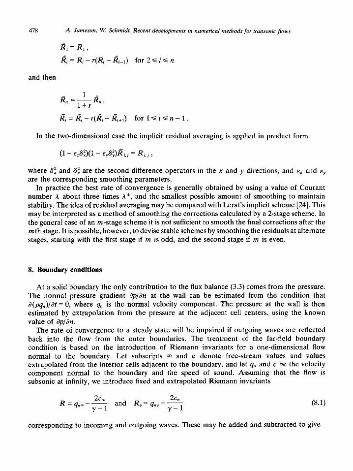
We first present a result for a classical test case, the Burgers’ equation, to demonstrate the efficiency of the METS (~ultig~d Explicit Time Stepping) scheme, Fig. 1 presents results for a


Final state of Burger’s equation after 20 cycles of the multigrid scheme

Residual .5327 10-g

Inftial state and first 10 cycles in evolution of Burger’s equation (reading upwarde)

Adaptive dissipation (scheme la) 128 cells 5 grids A - 2.0

Fig. 1. Solution of Burgers’ equation METS scheme.

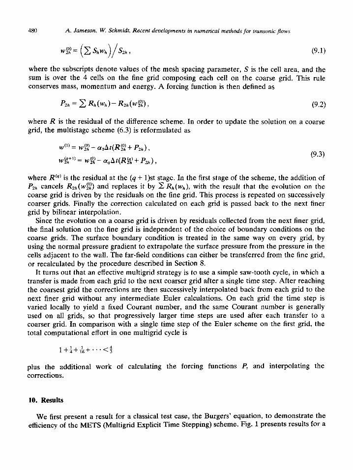
SUBSONIC SUBCRITICAL EULER SOLUTIONS DO AGREE WITH THE

FULL POTENTIAL SOLUTION ON THE SANE MESH

EXAMPLES: NACA %12, M = 0.5, = = 3’

RAE 2822, M = 0.50, Q = 3’

Fig. 2. Comparison of potential and Euler solution for subsonic flow.


symmetric jump using the adaptive dissipation discussed in Section 4. The TVD scheme of Section 5 gave essentially the same results, but was slightly slower in convergence.

We present a selection of results obtained for two- and three-dimensional flows. So far a wide range of configurations from airfoils to air intakes, diffusers, cascades, bodies, wings, road vehicles, and wing-body-tail combinations have been analyzed. Some of these ap- plications can be found in [g-11, 27-311. The main objective of the results discussed here is to validate the numerical solutions of the Euler equations. Our first step is to compare subsonic Euler solutions with potential flow solutions since both should agree exactly in two-dimensional flow. Fig. 2 compares the non-lifting flow over a circular cylinder at A4 = 0.20 and lifting airfoil flow at A4 = 0.50. In all cases meshes of O-structure with 128 x 32 volumes have been used for both solutions. The agreement proves to be quite good.

Fig. 3 presents numerical results on a 192 x 32 grid for the shock-free Korn airfoil. For the same flow condition both, the Euler and the full potential solution, are shock-free and give

COMPARISON FULL POTENTIAL - EULER SOLUTION

MESH EULER FULL POTENTIAL

_A

SHOCK-FREE KORN-AIRFOIL

Fig. 3. Comparison of Euler and potential solution for transonic shock-free flow.

SHOCK FREE NLR 7301 BOERSTOL-DESIGN

MESH PRESSURE DlSTRlSUTlON ISO-MACHLINES

Fig. 4. Comparison of Euler solution with transonic hodograph design.


almost the same results. The comparison for the shock-free NLR 7301 Boerstol hodograph design in Fig. 4 also proves the high accuracy of the presented Euler solution.

Let us now draw our attention to transonic flows with shocks. Fig. 5 portrays results for the NACA 64 A 401 airfoil section at M = 0.720 and zero-degree angle of attack. Both results look quite similar, however, the lift coefficient C, is less in the Euler solution and the shock is slightly further upstream. For flows with stronger shocks this difference can become quite large as shown in Fig. 6 for the NACA 0012 section. Now the lift is almost 30% smaller in the Euler solution. The mechanism for this disagreement is quite well understood and depends on the

CONPARISON FULL POTENTIAL - EULER FOR FLOWS WITH SHOCKS

SAME 192 x 32 MESH FOR NACA 64 A 410

Fig. 5. Comparison of potential and Euler solution for transonic airfoil flow with a shock. Left: potential solution; M = 0.720, a: = 0, CL = 0.664, CD = 0.0031. Right: Euler solution; h4 = 0.720, ty = 0, CL = 0.628, CD = 0.0035.

. . I

: * N4:fi X:2

?lacLc

; CL a.753 :_=*4 2. ccc

0.5i32 :2 C.OZlS CM -0.0325 iRIO ISiU?i %CYC 2s scso. t635-0:

. . . . . *--....__

_.-- -... :

-.‘=q,

* a’ -3% . l

l * ‘

.

.- Y 6

. .

8 . I = : -

NRCQ 5512 .

ns:n 0.755 QLPHFI 2. t)JO

?.J ! CL 0.1341 :3 0.0129 cm CR10 152x32

-O.OilSS hCTC SO ~ES0.82Y0-OU

Fig. 6. Comparison of potential .and Euler solution for lifting transonic flow with a strong shock. Left: potential solution; M = 0.75, CL = 0.6132, CD = 0.0215. Right: Euler solution; M = 0.75, CL = 0.4341, co = 0.0129.


overprediction of the shock jump in isentropic potential flow and on the lack of total pressure losses behind shocks, causing different trailing edge flows conditions as discussed in [S].

Looking at Fig. 7 we can analyze the total pressure losses for the numerical solution of the Euler equations over the RAE 2822 section in more detail. The plot of total pressure losses should show no losses except at the shock. However, the strong expansion of the flow over the highly curved leading edge produces some small losses because of discretization errors in the

O-MESH:

C-MESH:

- BOUNDARY CONDITIONS

- DISSIPATIVE TERMS

- MESH FUNCTION-GRADIENTS

Fig. 7. Accuracy of numerical Euler solutions.

. . . . ..- ,.....

: ./ . . . .

..: 2:~ :.:.

/.. -.., . :

x.., .:

;. ./

‘...,. . . . .

. . ..‘I.

3. :

r : . WI) Doll .

I 5 FY 0”s :,‘” “rso o.on, -’ WI0 ,‘a”,? *c,c 100 :h.. i%z 0 CP-PLOTS INDICATES DIFFERENT TRAILING EDGE RESOLUTION,

HOWEVER MINOR INFLUENCE ON TOTAL FORCES !

Fig. 8. Mesh influence on numerical Euler solution.


equations, geometry and boundary conditions. We found the amount of adaptive dissipation as discussed in Section 4 to be less important for the numerical total pressure losses at the nose than the mesh spacing or the boundary condition discretization. The oscillation in total pressure loss across the shock jump is caused by the small amount of numerical dissipation used.

Within the design principles for our method the numerical solution should not depend on the type of mesh but only on the numerical discretization, e.g. the number of mesh points on the surface. Fig. 8 verifies this by comparing the solutions using the same method but two different mesh types. The results are quite similar except for the trailing edge since the mesh spacing in a C-mesh is by definition coarser at the trailing edge. Fig. 9 gives a nice example of convergence to one solution with mesh refinement. From these results it can be also concluded that for engineering purpose meshes like 160 X 32 or sometimes even 80 x 16 can be good enough to give qualitative results in pressure: however, total force prediction may require finer meshes. To show the flexibility of the present schemes, a first result using triangular meshes is presented in Fig. 10. More information on this version will be published in [32].

Fig. 11 presents the typical convergence behavior of the present METS (multigrid explicit

CP(X,CI 2.N NLR 73GI

Oa5997 1 0,0004 I- r),1323 I I

-1 Fig. 9. Convergence of solution with

U’&R 73”: M=S.l 213 Ai_PHR=-0.194 I

MESHES LIKE 160 X 32 GIVE GOOD

RESULTS: METHOD CONVERGENCES

WITH MESH REFINEMENT,

mesh refinement.


time stepping) scheme. On 160 X 32 meshes for a wide range of airfoil problems converged solutions can be obtained after 25-50 cycles requiring lo-20 CPU seconds on a CRAY-1S computer. Fig. 12 portrays typical results for a super-fine mesh. This rather difficult case with a shock on upper as well as lower surface converges on a 320 x 64 grid very rapidly. The solution

Fig. 10. Euler solution for transonic

++ ++++++++

&

0012 0.800

0.0

+ + + +

l

+

+

l

*

+

:: + + L

ALPHR 0.0 co 0.0085

airfoil flow using triangular mesh discretization.

160 x 32 grid

CL .6292 CD .0036 25 cycles Residual .248 1O-3

Fig. 11. Convergence behavior of METS scheme for transonic airfoil flows.

A. Jameson, W. Schmidt, Recent developments in numerical methods for tnznsonic flows

;,

i

i I

t I

x/c O.00 0.80 C.YC 0.60 , o;oc 1:CI

: 1. -PI/PIINF Vs. X/f ON NC:? St:2

Fig. 12. Solution for super-fine meshes.

in pressure is converged already after 100 cycles, while the very accurate total pressure loss results as shown in Fig. 12 require at least 200 cycles. After 500 cycles the residuals are less than 10-l’ in density and less than lo-l2 in total enthalpy. The CPU time was 100 set for 100 cycles on a CRAY-1s. A typical result for internal compressible flows is shown in Fig. 13 for a duct at two different pressure ratios and for an entrance Mach number of 0.60.

From the range of three-dimensionai resuhs obtained so far with this method (see e.g. [9-l& 29-31]), t wo wing examples are presented that were testcases in the AGARD FDP Working Group 07. Fig. 14 presents results for the high aspect ratio transport-type wing, while Fig. 15 shows results for a low aspect ratio fighter-type wing with leading edge vortex flow. These examples are representative of the type of information about shocks and vortex structure that Euler methods can provide.

We finally provide some info~ation about the more recent extensions of the present Euler


Fig. 14. Euler solution for a transonic transport wing.

methodology to efficient Navier-Stokes methods. By adding the viscous stress tensor fluxes to the pressure terms in the momentum and energy equations any Euler method can be changed to a Navier-Stokes method in principle. For turbulent flows, in addition, a turbulence model has to be provided to model the time-averaged turbulent flow quantities. All methods discussed here use the algebraic models of Cebeci-Smith, BaIdwin-Lomax, or modifications. Fig. 16 presents a result for the RAE 2822 airfoil section which was originally published in [33]. Here the standard scheme without multigrid has been used. The agreement with experimental data looks quite promising. Fig. 17 shows results again using the scheme without multigrid, but this time in a multiblock structured version to allow high resolution out of core solutions. Details of this car analysis work can be found in [34]. More recently we succeeded in

TRANSONIC LEADING EDGE VORTEX FLOW

t

ISOBARS ON TUE uffa WRFA~X OF D~LLNER WIND DiLLNER WING CROSSPLlVJE u - 0.7.0 * ~6.Ol vELoClTIEs w - 0.7.0 * 1s.w

Fig. 15. Solutions for slender wings without and with body with leading edge vortex flow.

Experiment NASA CR-2610

. 1042 * = 0.50

o = 0.64

4 = 0.65

n = 1.00

&I = 0.4

<, = 160 \

a me56ure#en~ lower surface A uppe surf ace

- present results: N initially spaced points - odopted grid

j RAE 2822 - case 9

lo. 00 0.25 0.50 0.75 1.00 x/c

Fig. 16. Time-stepping solution for turbulent Navier-Stokes equation.

490

8

? ,

8

FIG. : CP(X/Cl ON NWA 0012


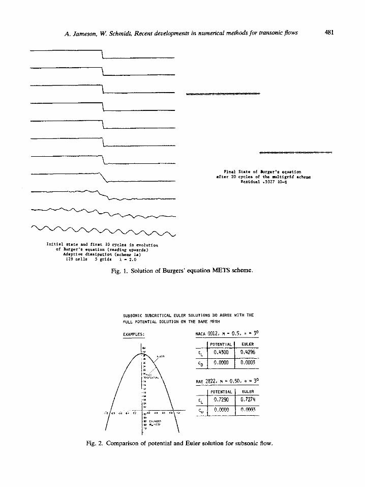
TURBULENT BLUFF BODY FLOW SI'IULATION

0 R-K TIME STEPPING SCHEME IN BLOCK STRUCTURES MESH

o MOVlNG OR FIXED GROUND SIMULATION GIVES SIGNIFICANT DIFFERENCES

0 IS WAKE STEADY ?

Fig. 17. Navier-Stokes solution for car center-section.

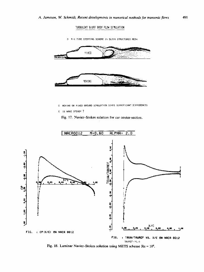
1 NACA0012 II=O. 60 ALPHA= 2.0

X/C Opll , 6,66 , $60 , 0,60 , op , I,66

FIG. t TBUWTAUREF VS. X/C ON NACR 0012

TRUREF-25.0

Fig. 18. Laminar Navier-Stokes solution using METS scheme Re = 10’.


applying the multigrid technique to solutions of the two-dimensional Navier-Stokes equations. The scheme used is exactly the same as discussed previously. Some first results are presented in Fig. 18, details can be found in [35]. The acceleration obtained so far by using multigrid for the Navier-Stokes equations is not as dramatic as for the Euler equations stemming from the high-resolution fine mesh close to the wall and the corresponding mesh stretching. Further work has to be done to analyze and improve the multigrid scheme.

References

[1] A. Jameson, W. Schmidt and E. Turkel, Numerical solution of the Euler equations by finite volume methods using Runge-Kutta time stepping schemes, AIAA Paper 81-1259, 1981.

[2] A. Harten, P. Lax and B. van Leer, On upstream differencing and Godunov type schemes for hyperbolic conservation laws, SIAM Rev. 25 (1983) 35-61.

[3] S. Osher and S. Chakrav~thy, High resolution schemes and the entropy condition, ICASE Rep. NASA CR 172218, 1983.

[4] P.L. Roe, The use of the Riemann problem in finite difference schemes, in: W.C. Reynolds and R.W. MacCormack, eds., Proc. 7th International Conference on Numerical Methods in Fluid Dynamics, Stanford, 1980 (Springer, Berlin, 1981) 354-359.

[S] P.L. Roe, Approximate Riemann solvers, parameters vectors, and difference schemes, J. Comput. Phys. 43 (1981) 357-372.

[6] J.P. Veiullot and H. Viviand, Methods pseudo-instationnaire pour l’calcul d’ecoulements transoniques, ONERA Publication 1978-4, 1978.

[7] W. Schmidt and A.W. Rizzi, Study of Pitot-type supersonic inlet-flowfields using the finite volume approach, AIAA Paper 78-1115, 1978.

[8] W. Schmidt, A. Jameson and D. Whitfield, Finite volume solutions to the Euler equatons in transonic flow, J. Aircraft 20 (2) (1983) 127-133; also AIAA Paper 81-1265, 1981.

[9j W. Schmidt and A. Jameson, Recent developments in finite volume time dependent techniques for two and three dimensional transonic flows, Von Karman Institute Lecture Series 1982-04, 1982.

[lo] A. Jameson and T.J. Baker, Solution of the Euler equations for complex configurations, Proc AIAA 6th Computational Fluid Dynamics Conference, Danvers (1983) 293-302.

Ill] S. Hitzel and W. Schmidt, Slender wings with leading-edge vortex separation: A challenge for plane methods and Euler solvers, J. Aircraft 21 (10) (1984) 751-759; also AIAA Paper 83-0562, 1983.

[12] J.P. Boris and D.L. Book, Flux corrected transport, 1, SHASTA, a fluid transport algorithm that works, J. Comput. Phys. 11 (1973) 38-69.

1131 S. Zalesak, Fully multidimensional flux corrected transport algorithm for fluids, J. Comput. Phys. 31 (1979) 335-362.

[14] A. Harten, High resolution schemes for hyperbolic conservation laws, New York University Rept. DOE/ER 030’77-175, 1982.

[lS] P.D. Lax, Hyperbolic systems of conservation laws and the mathematical theory of shock waves, SIAM Regional Series on Applied Mathematics 11, 1973.

[16] A. Jameson and P.D. Lax, Conditions for the construction of multi-point total variation diminishing difference schemes, Princeton University, Rept. MAE 1650, 1984.

f17j S. Osher, Riemann solvers, the entropy condition, and difference approximations, SIAM J. Numer. Anal., to appear.

[18] B. van Leer, Towards the ultimate conservative difference scheme, II. Monotonicity and conservation combined in a second order scheme, J. Comput. Phys. 14 (1974) 361-370.

[19] J.B. Goodman and R.J. Leveque, On the accuracy of stable schemes for 2-D scalar conservation laws, Math. Comput., to appear.

[20] A. Jameson, Numerical solution of the Euler equations for compressible inviscid fluids, Princeton University, Rept. MAE 1643, 1984.


[21] P. van der Houwen, Construction of Integration Formulas for Initial Value Problems (North-Holland,

Amsterdam, 1977). [22] P. Sonneveld and B. van Leer, Towards the solution of van der Houwen’s problem, Nieuw Archief voor

Wiskunde, to appear. 1231 P.L. Roe and J. Pike, Restructuring Jameson’s finite volume scheme for the Euler equations, RAE Rept.,

1983. [24] A. Lerat, J. Sides and V. Daru, An implicit finite volume scheme for solving the Euler equations, in: E.

Krause, ed., Proc. 8th International Conference on Numerical Methods in Fluid Dynamics, Aachen, 1982

(Springer, Berlin, 1982) 343-349.

[25] R.H. Ni, A multiple grid scheme for solving the Euler equations, Proc. AIAA 5th Computational Fluid

Dynamics Conference, Palo Alto, CA (1981) 257-264. [26] A. Jameson, Solution of the Euler equations by a multigrid method, Appl. Math. Comput. 13 (1983) 327-356.

[27] H.C. Chen, P. Rubbert, N.J. Yu and A. Jameson, Flow simulation for general Nacelle configurations using

Euler equations, AIAA Paper 83-0.539, 1983. [28] D. Whitfield and A. Jameson, Three dimensional Euler equation simulation of propeller-wing interaction in

transonic flow, AIAA Paper 83-0236, 1983. [29] J. Grashof, Numerical investigation of three dimensional transonic flow through air intakes distributed by a

missile plume, AIAA Paper 83-1854, 1983.

[30] B. Wager and W. Schmidt, Advanced numerical methods for analysis and design in aircraft aerodynamics,

ICAS-84-1.1.2, 14th Congress, Toulouse, September 1984.

[31] A. Jameson, R.W. MacCormack and W. Schmidt, Using Euler solvers, AIAA Professional Study Seminar, Snowmass, June 1983.

[32] A. Jameson and D. Mavriplis, Finite volume solutions of the two dimensional Euler equations on a regular triangular mesh, AIAA Paper 85-0435, January 1985.

[33] W. Haase, B. Wagner and A. Jameson, Development of a Navier-Stokes method based on a finite-volume technique for the unsteady Euler equations, Proceedings of the 5th GAMM Conf. on Numerical Methods in Fluid Mechanics, Rome, (Vieweg Verlag, Braunschweig, 1983).

[34] W. Fritz, Calculations of 2-D flows around car-shaped bodies in ground effect, Dornier Report, 1984.

[35] A. Jameson and W. Schmidt, Numerical solutions of the Navier-Stokes equations for compressible flows using multigrid-time-stepping schemes, AIAA/DGLR Study Seminar ‘Using Euler Solvers’, Stuttgart, January 1985.

some recent developments in numerical methods...

Documents