Some questions of control in fluid mechanics

Olivier Glass

CeremadeUniversité Paris-Dauphine

CIME – Control of Partial Differential Equations,Cetraro, July 2010.

Introduction

Control systems

DefinitionA control system is an evolution equation (ODE, PDE) depending on aparameter u:

y = f (y , u), (CS)

whereI y ∈ Y is the unknown, call the state of the system,I u ∈ U is the parameter called the control, that one can choose as a

function of the time.

Typically:I y(t) ∈ Rn, u(t) ∈ Rm, and (CS) is an ODE, orI y(t) and u(t) belong to some functional spaces and (CS) is a PDE

(so f is an operator).

Goal: to influence the dynamics of the system in a prescribed manner, bychoosing the control in a relevant way.

An example of control systemBoundary control of Navier-Stokes. Consider Ω a bounded domain, and anon empty open part of the boundary Σ ⊂ ∂Ω. Consider theNavier-Stokes equations, the control acting as a boundary conditionlocated in Σ: ∂tv + (v · ∇)v − ν∆v +∇p = 0,

div v = 0v|∂Ω = 1Σ(x)u(t, x).

I The state is the velocity field v ,I the control is the localized boundary term u = u(t, x).

Ω Σ

I Many other examples in fluid mechanics!I Many other ways the control could act on the fluid...

Examples of questions of controlMany different type of questions can be raised in the context of controlsystems.

I Optimal control. One looks for a control the minimizes some costfunction, e.g.

J(u) = ‖y(T ; u)− y‖2 + ‖u‖2,

where y is some target and y(T ; u) is the state reached by thesystem, starting from y0 and with control u.

I Exact controllability. Given T > 0, y0 and y1 two possible states ofthe system, does there exist u : [0,T ]→ U such that

y|t=0 = y0, y = f (y , u) =⇒ y(T ) = y1?

Y

y0y1

t0 T

Examples of questions of control

I Many other types of controllability. . .

I Asymptotic stabilization. Given an equilibrium state (ye , ue), canone find a state feedback function u = u(y), such ue = u(ye) thatthe so-called closed-loop system:

y = f (y , u(y)), (CLS)

is (locally) asymptotically stable at the point ye , i.e.I ∀ε > 0, ∃η > 0, all solution starting from y0 ∈ B(ye , η) are global

and satisfy ∀t ≥ 0, y(t) ∈ B(ye , ε),I any such solution satisfies y(t)→ ye as t → +∞?

I . . .

RemarkThese properties can be local (satisfied for y1 sufficiently close to y0 ory(T ) or ye) or global (satisfied without such constraint).

A reference

Many problems of control in fluid mechanics were raised in

Jacques-Louis Lions, Are there connections between turbulence andcontrollability?,published in Analysis and Optimization of Systems, 9th InternationalINRIA Conference (Antibes, June 12-15, 1990), A. Bensoussan and J.-L.Lions, eds., Lecture Notes Control and Inform. Sci. 144, Springer-Verlag,Berlin, 1990.

Different topics

I Euler equation for incompressible fluids

I Exact controllability for the incompressible Euler equation

I Lagrangian approximate controllability for the Euler equation

I Controllability of the 1D isentropic (compressible) Euler equation

I Controllability in the vanishing viscosity limit (1D models)

Exact controllability of the Euler equation

I. IntroductionI We consider a smooth bounded domain Ω ⊂ Rn, n = 2 or 3.

I Euler equation for perfect incompressible fluids∂tv + (v .∇)v +∇p = 0 in [0,T ]× Ω,div v = 0 in [0,T ]× Ω.

I Here, v : [0,T ]× Ω→ R2 is the velocity field, p : [0,T ]× Ω→ R isthe pressure field.

I To close the system, one adds the non-penetration condition on theboundary:

v .n = 0 on [0,T ]× ∂Ω,

with n the unit outward normal on ∂Ω.

I ⇒ global (resp. local) well-posedness of the system in 2D (resp.3D), cf. Lichtenstein, Wolibner, Yudovich, Kato, Ebin-Marsden, etc.

Boundary controlI We consider a non empty open part Σ of the boundary ∂Ω.

I Non-homogeneous boundary conditions can be chosen as follows:I on ∂Ω \ Σ, the fluid does not cross the boundary, v .n = 0.

I on Σ, we suppose that one can choose the boundary conditions, thatis, use them as a control.

Ω Σ

I As non-homogeneous boundary conditions one can choose forinstance:

I in 2D (Yudovich):v(t, x).n(x) on [0,T ]× Σ,

curl v(t, x) on Σ−T := (t, x) ∈ [0,T ]× Σ / v(t, x).n(x) < 0 .

I in 3D (Kazhikov):v(t, x).n(x) on [0,T ]× Σ,

curl v(t, x) ∧ n on Σ−T := (t, x) ∈ [0,T ]× Σ / v(t, x).n(x) < 0 .

The problem of exact controllability

I Standard problem of exact controllability:

Given T > 0, v0, v1 satisfying compatibility conditions, can one finda boundary control such that the solution satisfies

v|t=0 = v0 and v|t=T = v1?

I Alternative formulation:

Given v0, v1 and T as above, can one find a solution of the equationsatisfying the constraint on the boundary:

v .n = 0 on [0,T ]× (∂Ω \ Σ),

(under-determined system) and driving v0 to v1 at time T?

→ the control is obtained as the trace of v . . .

Exact controllability results

Theorem (Coron)The 2-dimensional Euler equation is exactly controllable in arbitrary timeif and only if Σ meets all the connected components of the boundary.

That is to say, under this condition, ∀T > 0, ∀v0, v1 ∈ C∞(Ω;R2), suchthat

div (v0) = div (v1) = 0 in Ω, v0.n = v1.n = 0 on ∂Ω \ Σ,

there exists v ∈ C∞([0,T ]×Ω;R2), solution of the system and satisfying

v|t=0 = v0 and v|t=T = v1.

Theorem (G.)The previous result also holds in 3-D.

Proof of the necessity of Σ meeting all the c.c. of ∂Ω

Two different conservations prove that if Σ does not meet all theconnected components of the boundary, then the controllability does nothold:

I 1. Kelvin’s law states that the circulation of velocity around aJordan curve is constant as the curve follows the flow.

But if such a curve belong to an “uncontrolled” component of ∂Ω, itwill stay on it, so that there has to be compatibility conditionsbetween v0 and v1.

I 2. In 2D, the vorticity ω := curl v follows the flow of v . In 3D itssupport does. And again an uncontrolled component of ∂Ω isconserved by the flow.

The problem of approximate controllability

I Standard problem of approximate controllability for the norm‖ · ‖W k,p :

Given T > 0 and v0 and v1 as above, ε > 0, can we find a controlsuch that the solution starting from v0 at time t = 0 satisfies attime t = T :

‖v(T , ·)− v1‖W k,p ≤ ε?

I Alternative formulation:

Given v0, v1 and T , can we find a solution of the under-determinedsystem with the boundary constraint:

v .n = 0 on [0,T ]× (∂Ω \ Σ),

and driving v0 at time 0 to a state at time T close to v1 in theprevious sense?

Approximate controllability results

Theorem (Coron)If Σ is non empty (but does not meet all the connected components ofthe boundary), the system is approximately controllable for the normLp(Ω), p <∞. Not for p =∞.

Theorem (G.)If v0 and v1 have the same velocity circulation on the uncontrolledcomponents of the boundary, then the approximate controllability occursin W 1,p, p <∞. Not for p =∞.

If moreover there exist smooth deformations on these componentssending the vorticity distributions of v0 on the ones of v1, then theapproximate controllability occurs in W 2,p, p <∞. Not for p =∞.

RemarksI What happens next (e.g. for W 3,p) is open.I The 3-D case is still open when Σ does not meet all the connected

components of the boundary.

II. Proof of the exact controllability

I The most standard method to prove controllability of a nonlinearPDE is the following.1. Linearize the equation,2. Prove a controllability result on the linearized equation,3. Deduce a controllability result on the nonlinear system

I To prove the controllability of the linearized equation, there is astandard approach by duality (D. Russell, J.-L. Lions).

This consists in proving an observability inequality on the(homogeneous) dual system.

(One has to prove the surjectivity of the control 7→ final state map,and the argument is somewhat close to the standard

A surjective ⇐⇒ ∃c > 0, ∀u, ‖A∗u‖ ≥ c‖u‖.)

I However, this method has at least two drawbacks:

I Frequently, this only leads to local results, unless the nonlinearity isnice (see e.g. Zuazua 1988),

I In many physical cases, and in particular for what concerns the Eulerequation, the linearized equation is not (systematically) controllable.

I Linearized Euler equation around 0:∂tv(t, x) +∇p(t, x) = 0 in [0,T ]× Ω,div v(t, x) = 0 in [0,T ]× Ω.

I This equation is not controllable, because

v|t=T − v|t=0 is the gradient of a harmonic function.

The return method

A method designed by J.-M. Coron to tackle this kind of situation is thereturn method. The idea is the following

Find a particular solution y of the (nonlinear) system, such thaty(0) = y(T ) = 0 and such that the linearized system around yis controllable.

state space

t

T

y

solution of thecontrollability problem

v0 v1

→ One may hope to find a solution of the nonlinear controllabilityproblem close to y .

The choice of y : what should it do?I Let ω := curl (v) the vorticity (either a scalar in 2D or a vector in

3D)I It satisfies

∂tω + (v · ∇)ω = 0 (2D)

or∂tω + (v · ∇)ω = (ω.∇)v (3D).

I Hence the vorticity follows the flow of v (2D), or, at least, itssupport does (3D).

I If one wants to steer y0 to y1 = 0, with curl (y0) 6= 0 on Ω, even if‖y0‖ 1, one should expect:

the flow of y makes every point of Ω leave the domain.

The choice of y : what can it do?I How to construct a solution of the nonlinear system (with control)?

I A very classical form of particular solutions is given by potentialflows:

y(t, x) = ∇xθ,

where∆xθ(t, x) = 0 for all (t, x) ∈ [0,T ]× Ω.

I These are solutions of the Euler equation: take

p = −θt −|∇θ|2

2.

I The boundary condition translates into

∂nθ(t, x) = 0 for all (t, x) ∈ [0,T ]× (∂Ω \ Σ).

Construction of y

Proposition 1There exists θ ∈ C∞([0,T ]× Ω;R) such that

∆xθ(t, x) = 0 in [0,T ]× Ω, ∂nθ(t, x) = 0 on [0,T ]× (∂Ω \ Σ), (1)

such that the flow of ∇θ makes all the points in Ω leave the domain.

I Remark: extend θ into a function of C∞([0,T ];C∞c (Rn)) to definea flow globally.

I This proposition is the consequence of the following one:

Proposition 2Given a curve γ ∈ C k([0, 1]; Ω), there exists θ ∈ C k([0, 1]× Ω;R)satisfying (1) such that the flow Φ of ∇θ satisfies:

Φ(t, 0, γ(0)) = γ(t).

The same holds for γ ∈ C∞([0, 1]; ∂Ω).

Construction of y , 2I Once Proposition 2 is proved, the function θ is obtained by gluing in

time several flows of this type: θ1( tε , x) during [0, ε], then

−θ1( 2ε−tε ) during [ε, 2ε], then θ2( t−2ε

ε , x) during [2ε, 3ε], then−θ2( 4ε−t

ε ) during [3ε, 4ε], etc.

Σ

Φ∇θ1

Φ∇θ2

Φ−∇θ2

Φ−∇θ1Ω

and use the compactness of Ω.

Following a curveI To prove that any curve can be achieved by the trajectory of a

potential flow, we use the following lemma.

LemmaOne has the following:∇θ(x), θ ∈ C∞(Ω;R) satisfying (1)

=

Rn for x ∈ Ω ∪ Σ,Tx∂Ω for x ∈ ∂Ω \ Σ.

I Then one can find a finite number of functions satisfying (1), suchthat

∀t ∈ [0, 1], Span∇θ1(γ(t)), . . . ,∇θN(γ(t)) = Rn (or Tγ(t)∂Ω).

I Then one can construct θ(t, x) with the form

θ(t, x) =N∑

i=1

ρi (t)θi (x).

by using the compactness of [0, 1] and a partition of unity.

Proving the lemmaI In 2D, this can be proved by using Runge’s theorem. Indeed, in

dimension 2, complex analysis is very useful to construct such flowsbecause, setting Vf := (Re f ,−Im f ):

f satisfies the Cauchy-Riemann equations⇐⇒ curl Vf = div Vf = 0,

pole

ϕ = 0

Ω

ϕ = c

I Approximate ϕ definedas on the left, by arational function with apole /∈ Ω,

I Subtract a smallsolution of a Neumannproblem to get ∂nθ = 0exactly.

Proving the lemma, 2I If x ∈ ∂Ω \ Σ, the situation is more difficult. Instead of

approximating 0 near ∂Ω \ Σ, approximate

N(a)

[1

z − a− 1

z − a

], as a→ x ,

where N(a) = O(d(x , a)) is a suitable normalization factor and a, aare as in the following figure.

poleΩ

xa

a

Using the function y

I We first consider the case where v0 is small enough (in some norm),and v1 = 0. The general case will be deduce from this particularone.

I Let us also suppose that Ω is simply connected.

I Given such v0, we try to construct by standard arguments in fluidmechanics a solution of the system:

curl (v) = ω in [0,T ]× Ω,div (v) = 0 in [0,T ]× Ω,v .n = ∇θ.n on [0,T ]× ∂Ω,

∂tω + (v .∇)ω = 0 in [0,T ]× Ω,ω|t=0 = ω0 in Ω,ω = 0 on (t, x) ∈ [0,T ]× Σ / ∇θ.n < 0.

(We put aside the regularity/compatibility conditions issues.)

Using the function y , 2

I Now, if ‖v0‖ 1, the solution will be close to the one obtained withy0 = 0.

I This solution is precisely y .

I Hence, for ‖v0‖ small enough, the flow of v makes all points in Ω att = 0 leave the domain.

I Hence, ω(T ) = 0.

I Bring v .n back to 0, and since Ω is simply connected, we havefinished.

How to make the construction smoothNow, to do this in a smooth manner:

I Extend the velocity field v (close to ∇θ) to v on R2 with compactsupport.

I Transport the vorticity by v , and a finite number of times, transformthe vorticity by

ω(t+, x) = ϕ(x)ω(t−, x),

where ϕ is a cutoff function such that ϕ = 1 on Ω.

I Inside Ω, the solution is smooth. . .

Places where the cutoffΦ∇θ2

Φ−∇θ2

Φ−∇θ1

functions are 0

Ω Σ

Φ∇θ1

What if v1 6= 0 and v0 is not small?

I Now, if ‖v0‖ is not small, we use the time-scale invariance of theequation: for λ > 0,

v(t, x) is a solution of the equation defined in [0,T ]× Ω

⇐⇒ vλ(t, x) := λv(λt, x) is a solution of the equationdefined in [0,T/λ]× Ω.

I Hence, bringing v0 to 0 in time T is equivalent to bringing λv0 to 0in time T/λ.

I We know how to bring any v0 such that ‖v0‖ ≤ ε to 0 in time T .Hence we know how to bring any v0 with larger norm in smallertime.

I For what concerns v1 6= 0, use the reversibility of the equation: bringv0 to 0, and then 0 to v1.

What about multiply connected domains?

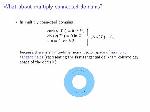
I In multiply connected domains,

curl (v(T )) = 0 in Ω,div (v(T )) = 0 in Ω,v .n = 0 on ∂Ω,

6⇒ v(T ) = 0,

because there is a finite-dimensional vector space of harmonictangent fields (representing the first tangential de Rham cohomologyspace of the domain).

What about multiply connected domains?, 2

I The solution consists in making vorticity pass across the domain asfollows:

I Hence one can fix the circulation of speed along a given family ofcurves; this suffices to get v(T ) = 0.

I One uses the principles showed above to do so.

What about 3D?There are three main differences for what concerns dimension 3.

I 1. Transport of the vorticity. Now the vorticity is no longertransported by the flow:

∂tω + (v .∇ω) = (ω.∇)v .

But its support is, and that suffices to our purpose.

But if such a curve belong to an “uncontrolled” component of ∂Ω, itwill stay on it, so that there has to be compatibility conditionsbetween v0 and v1.

I 2. Blow up. The solution could blow up (until proven otherwise).But mainly, we work with y0 such that ‖y0‖ ≤ ε. . .

In other words, we act sufficiently fast to avoid the blow up.

I 3. Topology. This is by far the most difficult issue.

What about 3D?, 2

I In 3-D, there exist Runge-type theorems of approximations ofharmonic functions by harmonic functions defined on a larger set:

Theorem (Walsh, 1929). Let K a compact set in Rn such thatRn \ K is connected. Then for each function u harmonic in an openset containing K , for each ε > 0, there exists a harmonic polynomialv such that

‖u − v‖∞ ≤ ε.

I The functions z 7→ 1z−a can be replaced by using the fundamental

solution of the Laplacian in R3.

What about 3D?, 3I In 3D, multiply connected domains can have connected boundary.

I To get rid of tangential harmonic vector fields, one uses vortexfilaments (or regularization of vortex filaments), that has to crossthe domain.

I One can check that the “change of velocity circulation” is given bythe intensity of the vortex filament.

I The main part consists in finding y whose flow make the vortexfilament cross the domain, using the previous tools.

Open problemsI Approximate controllability of the 3-D Euler equation. In dimension

3, if Σ 6= ∅ does not meet all the connected components of ∂Ω, theapproximate controllability in Lp is not known. The difficulty comesfrom a possible blow-up of the solution.

I Asymptotic stabilization by stationary feedback. Find a feedback lawwhich makes the closed-loop system asymptotically stable. Thesituation is well-understood in 2-D, cf. Coron, G.

But for what concerns the 3-D case, the problem is completely open.It is connected to the following problem.

Open question. Given Ω ⊂ R3 a smooth connected domain, andΣ 6= ∅ an open part of ∂Ω, does there exist θ ∈ C∞(Ω;R) such that

∆θ = 0 in Ω,∂θ∂n = 0 on ∂Ω \ Σ,|∇θ(x)| > 0 for all x ∈ Ω?

Some other references

I Navier-Stokes equations. For the Navier-Stokes equations, onewould like to show the controllability to trajectories. Several resultson this direction:

I Imanuvilov (2001), Fernandez-Cara-Guerrero-Imanuvilov-Puel(2004), local controllability to trajectories.

I Coron (1995), Coron-Fursikov (1996), Chapouly (2009): globalapproximate controllability, with Navier boundary conditions.(Relying on Euler!)

The problem of global controllability to trajectories of theNavier-Stokes equations with v = 0 on ∂Ω \ Σ is still open.

I Controllability by low modes. See Agrachev-Sarychev (2005),Shirikyan (2006), Nersesian (2010).

I . . .

Approximate Lagrangian controllabilityof the Euler equation

I. Introduction

I Again we consider a smooth bounded domain Ω ⊂ R2, and Σ anonempty open set of ∂Ω and the control system

∂tv + (v .∇)v +∇p = 0 in [0,T ]× Ω,

div v = 0 in [0,T ]× Ω,

v .n = 0 on [0,T ]× [∂Ω \ Σ].

I As previously the control is the boundary data on Σ, e.g.v(t, x).n(x) on [0,T ]× Σ,

curl v(t, x) on Σ−T := (t, x) ∈ [0,T ]× Σ / v(t, x).n(x) < 0 .

Another type of controllabilityI Another type of controllability is natural for equations from fluid

mechanics: is possible to drive a zone of fluid from a given place toanother by using the control? (Based on a suggestion by J.-P. Puel)

I One can think for instance to a polluted zone in the fluid, which wewould like to transfer to a zone where it can be treated.

I It is natural, in order to control the fluid zone during the wholedisplacement to ask that is remains inside the domain during thewhole time interval.

I Cf. Horsin in the case of the Burgers equation.

First definitionI Due to the incompressibility of the fluid, the starting zone and the

target zone must have the same area.I We have also to require that there is no topological obstruction to

move a zone to the other one.

I In the sequel, we will consider fluids zones given by the interior(inside Ω) of smooth (C∞) Jordan curves.

DefinitionWe will say that the system satisfies the exact Lagrangian controllabilityproperty, if given two smooth Jordan curves γ0, γ1 in Ω, homotopic in Ωand surrounding the same area, a time T > 0 and an initial datum v0,there exists a control such that the flow given by the velocity field drivesγ0 to γ1, by staying inside the domain.

An objection

The exact Lagrangian controllability does not hold in general, indeed:

I Let us suppose ω0 := curl v0 = 0. In that case if the flow Φ(t, x)maintains γ0 inside the domain, then for all t,

ω(t, ·) = curl v(t, ·) = 0,

in the neighborhood of Φ(t, γ0), since ω(t,Φ(t, x)) = ω0(x).

I Since div v = 0, locally around γ0, u is the gradient of a harmonicfunction; u is therefore analytic in a neighborhood Φ(t, γ0).

I Hence if γ0 is analytic, its analyticity is propagated over time.

I If γ1 is smooth but non analytic, the exact Lagrangian controllabilitycannot hold.

Approximate Lagrangian controllability

DefinitionWe will say that the system satisfies the property of approximateLagrangian controllability in C k , if given two smooth Jordan curves γ0,γ1 in Ω, homotopic in Ω and surrounding the same area, a time T > 0,an initial datum v0 and a real ε > 0, we can find a control such that theflow of the velocity field maintains γ0 inside Ω for all time t ∈ [0,T ] andsatisfies, up to reparameterization:

‖Φv (T , γ0)− γ1‖Ck ≤ ε.

Here, (t, x) 7→ Φv (t, x) is the flow of the vector field v .

Main result

Theorem (G.-Horsin)Consider two smooth smooth Jordan curves γ0, γ1 in Ω, homotopic in Ωand surrounding the same area. Let k ∈ N. We consider v0 ∈ C∞(Ω;R2)satisfying

div (v0) = 0 in Ω and v0.n = 0 on [0,T ]× (∂Ω \ Σ).

For any T > 0, ε > 0, there exists a solution v of the Euler equation inC∞([0,T ]× Ω;R2) with

v .n = 0 on [0,T ]× (∂Ω \ Σ) and v|t=0 = v0 in Ω,

and whose flow satisfies

∀t ∈ [0,T ], Φv (t, γ0) ⊂ Ω,

and up to reparameterization

‖γ1 − Φv (T , γ0)‖Ck ≤ ε.

A connected result: vortex patchesThe starting point is the following.

Theorem (Yudovich, 1961)For any v0 ∈ C 0(Ω;R2) such that div (v0) = 0 in Ω, v0.n = 0 on ∂Ω andcurl v0 ∈ L∞, there exists a unique (weak) global solution of the Eulerequation starting from v0 and satisfying v .n = 0 on the boundary.

A particular case of initial data with vorticity in L∞ is the one of vortexpatches.

DefinitionA vortex patch is a solution of the Euler equation whose initial datum isthe characteristic function of the interior of a smooth Jordan curve (atleast C 1,α).

Theorem (Chemin, 1993)In R2, the regularity of the boundary of the curve is propagated globallyin time.

Cf. also Bertozzi-Constantin, Danchin, Depauw, Dutrifoy, Gamblin &Saint-Raymond, Hmidi, Serfati, Sueur,. . .

Question: Can one control the shape of a vortex patch in a boundeddomain, by using a boundary control?

Control of the shape of a vortex patch

Theorem (G.-Horsin)Consider two smooth Jordan curves γ0, γ1 in Ω, homotopic in Ω andsurrounding the same area. Suppose also that the control zone Σ is inthe exterior of these curves. Let v0 ∈ Lip(Ω;R2) with v0.n ∈ C∞(∂Ω) avortex patch initial condition corresponding to γ0, i.e.

curl (v0) = 1Int(γ0) in Ω, div (v0) = 0 in Ω, v0.n = 0 on ∂Ω \ Σ.

Then for any T > 0, any k ∈ N, any ε > 0, there existsu ∈ L∞([0,T ];Lip(Ω)) a solution of the Euler equation such that

curl v = 0 on [0,T ]× Σ,

v .n = 0 on [0,T ]× (∂Ω \ Σ) and v|t=0 = v0 in Ω,

that Φv (T , 0, γ0) does not leave the domain and and that, up toreparameterization, one has

‖γ1 − Φv (T , 0, γ0)‖Ck ≤ ε.

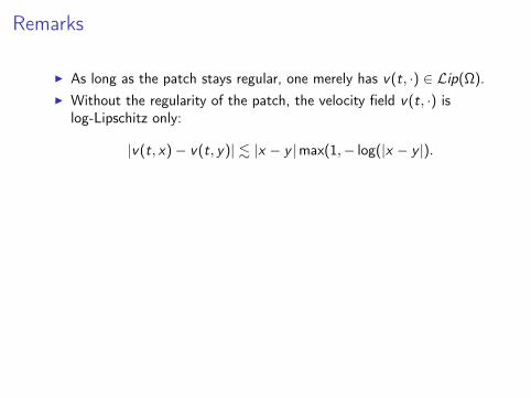
Remarks

I As long as the patch stays regular, one merely has v(t, ·) ∈ Lip(Ω).I Without the regularity of the patch, the velocity field v(t, ·) is

log-Lipschitz only:

|v(t, x)− v(t, y)| . |x − y |max(1,− log(|x − y |).

II. Ideas of proofI We exploit the same idea to use potential flows and complex

analysis.

PropositionConsider two smooth Jordan curves γ0, γ1 in Ω, homotopic in Ω andsurrounding the same area. For any k ∈ N, T > 0, ε > 0, there existsθ ∈ C∞0 ([0, 1];C∞(Ω;R)) such that

∆xθ(t, ·) = 0 in Ω, for all t ∈ [0, 1],

∂θ

∂n= 0 on [0, 1]× (∂Ω \ Σ),

whose flow satisfies

∀t ∈ [0, 1], Φ∇θ(t, 0, γ0) ⊂ Ω,

and, up to reparameterization,

‖γ1 − Φ∇θ(T , 0, γ0)‖Ck ≤ ε.

Ideas of proof for the main propositionI One seeks a potential flow driving γ0 to γ1 (approximately in C k)

and fulfilling the boundary condition on ∂Ω \ Σ.

I This is proven in two parts:

I Part 1: find a solenoidal (divergence-free) vector field driving γ0 toγ1.

I Part 2: approximate (at each time) the above vector field on thecurve (or to be more precise, its normal part), by the gradient of aharmonic function defined on Ω and satisfying the constraint.

Part 1

PropositionConsider γ0 and γ1 two smooth (C∞) Jordan curves homotopic in Ω. Ifγ0 and γ1 satisfy

|Int(γ0)| = |Int(γ1)|,

then there exists v ∈ C∞0 ((0, 1)× Ω;R2) such that

div v = 0 in (0, 1)× Ω,

Φv (1, 0, γ0) = γ1.

Cf. D.B.A. Epstein (1966), without the area/divergence constraint.

Ideas of proof for Part 1I The case where Int(γ0) and Int(γ1) do not intersect could be treated

rather simply.I But a way to treat the general case is to get in the opposite case:

Int(γ0) ∩ Int(γ1) 6= ∅.

It is enough to find a solenoidal vector field v diving a point of γ0 inInt(γ1), and to consider Φv (1, γ0) as a new initial curve.

I This is not difficult since any vector field of the form

v(t, x) = ∇⊥ψ(t, x) = (−∂x2ψ, ∂x1ψ),

is solenoidal.I Using a small translation if necessary, we can moreover suppose thatγ0 and γ1 intersect transversally.

Part 1, sequelI We are in the following situation (if fact, things can be way messier)

←−−→ γ0

↑γ1

↓

I We work on the symmetric difference of the two interiors.I The goal is, on each component of this symmetric difference, to find

a vector field who drives the segment of γ0 to γ1: inside Int(γ0)(purple zone) or Int(γ1) (green zone).

Part 1, sequelI On each component of the symmetric difference, we construct a

vector field driving the interval γk0 of γ0 on the interval γk

1 of γ1.

I A way to do this is to consider ∇ψ where ψ is the harmonicextension of a function equal to 0 (respectively 1) on the interval γk

0(resp. on the interval γk

1 ) and “regularized on the intersections”.

ψ = 0

γ0

γ1

ψ = 1

Part 1, endI Next we normalize the vector fields in order that the corresponding

flow, satisfies for t ∈ [0, 1]

Area(γk0 ,Φ(t, γk

0 )) = t Area(γk0 , γ

k1 ). (*)

I Then we have to glue these vector fields together, in a way that it issmooth at the points of γ0 ∩ γ1.

I Then, thanks to (*), the vector field restricted to (t,Φ(t, γ0)) canbe extended to a global solenoidal vector field.

Part 2

PropositionLet γ0 a smooth (C∞) Jordan curve; let X ∈ C 0([0, 1];C∞(Ω)) asmooth solenoidal vector field, with X .n = 0 on [0, 1]× ∂Ω. Then for allk ∈ N and ε > 0 there exists θ ∈ C∞([0, 1]× Ω;R) such that

∆xθ(t, ·) = 0 in Ω, for all t ∈ [0, 1],

∂θ

∂n= 0 on [0, 1]× (∂Ω \ Σ),

and whose flow satisfies

∀t ∈ [0, 1], Φ∇θ(t, 0, γ0) ⊂ Ω,

and, up to reparameterization,

‖ΦX (t, 0, γ0)− Φ∇θ(t, 0, γ0)‖Ck ≤ ε, ∀t ∈ [0, 1].

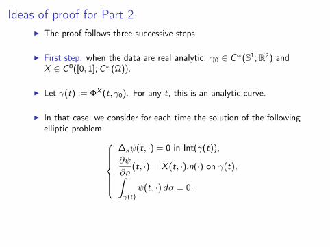
Ideas of proof for Part 2I The proof follows three successive steps.

I First step: when the data are real analytic: γ0 ∈ Cω(S1;R2) andX ∈ C 0([0, 1];Cω(Ω)).

I Let γ(t) := ΦX (t, γ0). For any t, this is an analytic curve.

I In that case, we consider for each time the solution of the followingelliptic problem:

∆xψ(t, ·) = 0 in Int(γ(t)),

∂ψ

∂n(t, ·) = X (t, ·).n(·) on γ(t),∫

γ(t)

ψ(t, ·) dσ = 0.

Part 2, sequelI As γ(t) and X .n on γ(t) are analytic, we can extend the solution ψ

across the boundary γ(t) (this is a Cauchy-Kowalewsky-style result).

I Using the continuity in time of X and γ with values in Cω, we seethat the size of the neighborhood of γ(t) where this solution can beextended can be estimated from below.

I With Runge’s theorem (of approximation of holomorphic functionsby rational functions) we can obtain approximations defined on Ω,and which satisfy

∇ψ(t, ·).n = 0 on ∂Ω \ Σ.

I We obtain the function θ as:

θ(t, x) =n∑

k=1

ρi (t)ψ(ti , ·),

with ρi a certain partition of unity of [0, 1].

Part 2, sequel

I Second step: when only the vector field is real analytic:X ∈ C 0([0, 1];Cω(Ω)) but γ0 ∈ C∞(S1;R2).

I We can approach γ0 (and γ1) by real analytic curves, from theoutside. This comes from a general result by H. Whitney, or in asimpler way in our case:

I We consider C0 the complement of Int(γ0) in the Riemann sphere.By Riemann’s conformal mapping theorem, there exists ϕ aconformal transformation from C0 in BC(0, 1).

I Then since such a conformal transformation is regular up to theboundary when γ0 is regular (Kellogg-Warschawski’s theorem), thecurve ϕ(S(0, 1− ν)) is an appropriate approximation.

Part 2, sequelI Next, we apply the process of Part 1 on the ν-approximations γν0

and γν1 of γ0 and γ1. We obtain a function θν .

I The central point is to show that, on Φ∇θν

(t, γ0), we have uniformestimates on ∇θν as ν → 0+.

I This comes from the construction and the fact that the constants inelliptic estimates in Int(γν) are bounded independently from ν.

I We conclude then by Gronwall’s lemma.

Part 2, sequel

I Third step: when both data are merely C∞: γ0 ∈ C∞(S1;R2) andX ∈ C 0([0, 1];C∞(Ω)).

I We use Whitney’s analytic approximation theorem: X can beapproached arbitrarily for the C 0([0, 1];C∞(Ω))-topology byX ν ∈ C 0([0, 1];Cω(Ω)).

I We conclude by using the previous step and Gronwall’s lemma.

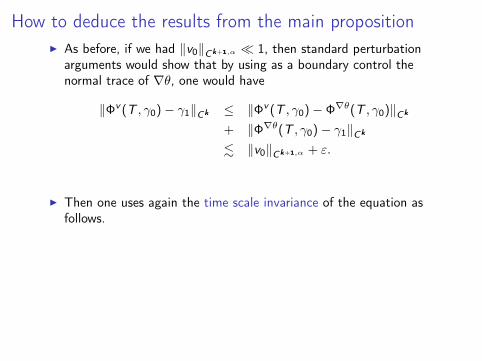
How to deduce the results from the main propositionI As before, if we had ‖v0‖Ck+1,α 1, then standard perturbation

arguments would show that by using as a boundary control thenormal trace of ∇θ, one would have

‖Φv (T , γ0)− γ1‖Ck ≤ ‖Φv (T , γ0)− Φ∇θ(T , γ0)‖Ck

+ ‖Φ∇θ(T , γ0)− γ1‖Ck

. ‖v0‖Ck+1,α + ε.

I Then one uses again the time scale invariance of the equation asfollows.

From the main proposition, sequelI We cut the time interval in the following way: for ν small:

time-scaled, where θ is such that

t = 0 t = T − ν t = T

γ0 := Φ(T − ν, γ0)

Φ∇θ(1, γ0) = γ1

Evolution ”without control” Control given by ∇θ

I In a first time, we “do nothing” (in fact, we have to take v0.n intoaccount).

I At the end of the time interval, we act fast and violently to driveΦ(T − ν, γ0) to γ1: with the control (mainly) given by the normalpart of 1

ν∇θ(t − T + ν, ·). The part of the control concerning thevorticity is just used in order not to ruin the regularity.

From the main proposition, sequel

I Let v be the resulting solution.

I If we change back the time scale to get back the dynamics of thetime interval [T − ν,T ] to the time interval [0, 1], the evolution isdriven by the Euler equation, with:

I As boundary condition (on the normal trace) the same as ∇θ

I As initial condition νu(T − ν, ·).

I ⇒ the initial datum is small!

I We show that the solution constructed on [0,T ]:

‖Φv (T , γ0)− γ1‖Ck . ν + ε.

The case of vortex patchesI The construction is similar, but we can no longer use

‖νu(T − ν, ·)‖Ck+1,α . ν,

because v is Lipschitz only!

I We use arguments due to:

I N. Depauw: vortex patches in a domain

I Bertozzi-Constantin, who tackled the problem of the regularity ofvortex patches by using the integro-differential equation satisfied bytheir boundary:

ddtγ(t, s) = − 1

2π

∫ 2π

0log |x − γ(σ)| τ(σ) dσ

+ here, terms due to the presence of ∂Ω and of the control.

What about 3D?I Several problems appear:

I How to deform (in a smooth, volume-preserving way) a domain toanother one?

I How to prevent the solution from potentially blowing up?

I The others parts of the proof do not depend on the dimension. . .

Proposition (G.-Horsin, in progress)If B1 and B2 are two smooth open sets in Ω, diffeomorphic to a ball, withsame volume, at positive distance from ∂Ω and disjoint, then one cansmoothly deform B1 to B2 inside Ω in a volume-preserving manner.

What about 3D, 2?

Corollary (G.-Horsin, in progress)Let B1 and B2 as previously, and S1, S2 their boundary. Let k ∈ N. Weconsider v0 ∈ C∞(Ω;R3) satisfying

div (v0) = 0 in Ω and v0.n = 0 on [0,T ]× (∂Ω \ Σ).

For any ε > 0, there exists T > 0 and a solution v of the Euler equationin C∞([0,T ]× Ω;R3) with

v .n = 0 on [0,T ]× (∂Ω \ Σ) and u|t=0 = v0 in Ω,

and whose flow satisfies

∀t ∈ [0,T ], Φv (t,B1) ⊂ Ω,

and up to reparameterization

‖S2 − Φv (T , S1)‖Ck ≤ ε.

Open problemsI More complex domains. What can be said if the fluid zone to be

displaced is no longer a Jordan curve, or about more generalsituations in 3D?

I Numerics. Can we find an efficient algorithm to compute thecontrol?

I Navier-Stokes equations. Can we obtain a similar result forincompressible Navier-Stokes equations?

∂tv + (v .∇)v −∆v +∇p = 0 in [0,T ]× Ω,div v = 0 in [0,T ]× Ω.

With Dirichlet’s boundary conditions? With Navier’s (cf. Coron,Chapouly)?

I Stabilization. Can we find a feedback control:

control(t) = f (γ(t), v(t)),

stabilizing a fluid zone at a fixed place?

Controllability of the 1D isentropic (compressible)Euler equation

I. Introduction

One-dimensional isentropic Euler equations:I In Eulerian coordinates:

∂tρ+ ∂x(m) = 0,∂t(m) + ∂x(m2

ρ + κργ) = 0.(EI)

I In Lagrangian coordinates:∂tτ − ∂xv = 0,∂tv + ∂x(κτ−γ) = 0. (P)

whereI ρ = ρ(t, x) ≥ 0 is the density of the fluid,

I m(t, x) is the momentum (v(t, x) = m(t,x)ρ(t,x) is the velocity of the

fluid),I τ := 1/ρ is the specific volume,I the pressure law is p(ρ) = κργ , γ ∈ (1, 3].

Controllability problem

I Domain: [0,T ]× [0, 1].

I State of the system:

Case (EI): u = (ρ,m), Case (P): u = (τ, v).

I Control: the “boundary data” (a delicate matter).

I Controllability problem: given u0 and u1, can we find a solution ofthe system driving u0 to u1?

Class of solutions

I Hyperbolic systems of conservation laws develop singularities infinite time.

I It is natural to consider discontinuous (weak) solutions which satisfyentropy conditions. Discontinuities appearing in the solutioncorrespond to shock waves.

I Here we consider BV solutions: solutions in L∞(0,T ;BV (R)) withsmall total variation and avoiding vacuum, constructed by a wavefront tracking algorithm.

II. Basic facts on systems of conservation lawsNotations:

I Systems of conservations laws:

ut + f (u)x = 0, f : Rn → Rn,

A(u) := df (u) has n real distinct eigenvalues λ1 < · · · < λn, withcorresponding eigenvectors ri (u).

I Genuinely non-linear fields in the sense of Lax:

∇λi .ri 6= 0 for all u.

⇒ we normalize ∇λi .ri = 1.I Case (EI): u = (ρ,m):

λ1 =mρ−√κγρ

γ−12 and λ2 =

mρ

+√κγρ

γ−12 ,

I Case (P): u = (τ, v):

λ1 = −√κγτ−γ−1 and λ2 =

√κγτ−γ−1.

Entropy solutions

I Entropy/entropy flux couple: (η, q) such that

∀u ∈ R+∗ × R, Dη(u).Df (u) = Dq(u).

I Entropy solutions:ut + (f (u))x = 0,

such that for all (η, q) entropy couple with η convex:

η(u)t + q(u)x ≤ 0.

I One can show that the solutions obtained by vanishing viscosity, i.e.as limits of solutions of

uεt + (f (uε))x − εuεxx = 0,

are entropy solutions.

Entropy solutions, 2

I In some sense, entropy solutions are solutions from which viscosityhas disappeared, except for what concerns the selection of admissiblediscontinuities.

I Glimm (1965) showed the existence of global entropy solutions withthe assumption of small total variation (under the GNL assumption).

I There is now a huge literature on the subject, and the situation isnow well understood in the context of small total variation. (See inparticular Bianchini-Bressan.)

The Riemann problem

I Find autosimilar solutions u = u(x/t) tout + (f (u))x = 0u|R− = ul and u|R+ = ur .

I Here ul and ur are constant states. This is a very particular case ofsolutions, which can be used as the elementary brick to constructgeneral solutions.

I Solved by introducing Lax’s curves which consist of points that canbe joined starting from ul either by a shock or a rarefaction wave.(The genuine nonlinearity is essential here.)

Shocks waves

I Shock waves are discontinuities at speed s satisfyingRankine-Hugoniot relations and Lax’s inequalities:

[f (u)] = s[u] (jump condition),λi (ur ) < s < λi (ul)

λi−1(ul) < s < λi+1(ur ).

ul ur

I The Rankine-Hugoniot ensure that this is a solution in the sense ofdistributions, Lax’s inequalities give the entropy criterion.

I There is a family of shocks associated to each characteristic family(i = 1, . . . , n).

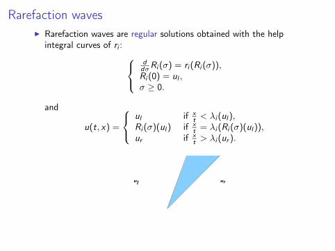
Rarefaction wavesI Rarefaction waves are regular solutions obtained with the help

integral curves of ri : ddσRi (σ) = ri (Ri (σ)),Ri (0) = ul ,σ ≥ 0.

and

u(t, x) =

ul if xt < λi (ul),

Ri (σ)(ul) if xt = λi (Ri (σ)(ul)),

ur if xt > λi (ur ).

ul ur

Lax’s curves

I Given ul , we associate:

I the curves of i-shocks, given by all states ur which can be connectedby ul through a shock of the i-th family,

I the curves of i-rarefactions, given by all states ur which can beconnected by ul through a rarefaction waves of the i-th family,

I Lax’s curves, obtained by gluing together these two curves.

I One can show that Lax’s curves are regular, because the i-shockcurves and the i-rarefaction curves have a second-order tangency atul (with suitable parameterization).

Lax’s curves, 2m

critical curve 2

2-shock1-shock

1-rarefaction

2-rarefaction

critical curve 1

ul

ρ

Lax’s curves in (ρ,m) coordinates

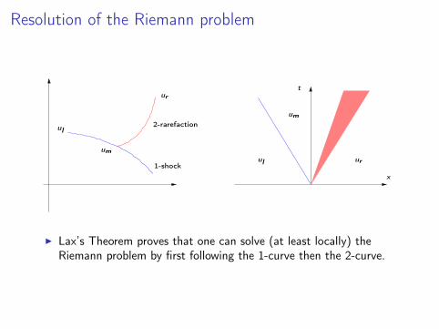
Resolution of the Riemann problem

ul

um

ur

1-shock

2-rarefaction

x

t

ul

um

ur

I Lax’s Theorem proves that one can solve (at least locally) theRiemann problem by first following the 1-curve then the 2-curve.

Riemann invariants

I w i is a i-Riemann invariant ⇐⇒ ri .∇w i = 0.

I Case (EI):

w1(u) =mρ

+2√κγ

γ − 1ργ−12 and w2(u) =

mρ−

2√κγ

γ − 1ργ−12 ,

I Case (P):

w1 = v +2√κγ

γ − 1τ−

γ−12 and w2 = v −

2√κγ

γ − 1τ−

γ−12 .

I It is interesting to parameterize wave curves by these Riemanninvariants.

Lax’s curves in Riemann coordinates

w1

vaccum

2-shock

1-shock

1-rarefaction

2-rarefaction

w2

Lax’s curves in (w1,w2) coordinates

Front-tracking algorithm (Dafermos, Di Perna, Bressan,Risebro, Ancona-Marson, . . . )

I This is a particular way to construct solutions to systems ofconservation laws (there are other ways, such as Glimm’s randomchoice method, the vanishing viscosity approach, etc.)

I The basic principle is:

I to construct a suitable sequence of piecewise constant functions overa polygonal subdivision of R+ × R,

I to prove estimates in L∞t (BVx) for the approximations,

I to extract a converging subsequence whose limit will be an entropysolution.

Front tracking algorithm, 2I Let ν > 0 (which will go to 0+).

I Approximate initial condition by piecewise constant functions:uν0 → u0 in L1

loc as ν → 0+.

I At each discontinuity of uν0 :I solve the corresponding Riemann problem,I replace rarefaction waves by rarefaction fans: these are piecewise

constant approximation in x−x0t with uk+1 = Ri (σ, uk) and

0 ≤ σ ≤ ν.t

x

ul

u3u2

ur = u4

um = u1

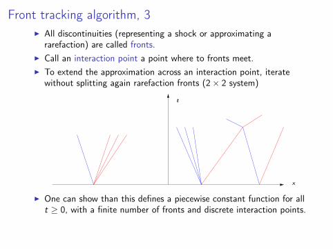
Front tracking algorithm, 3I All discontinuities (representing a shock or approximating a

rarefaction) are called fronts.I Call an interaction point a point where to fronts meet.I To extend the approximation across an interaction point, iterate

without splitting again rarefaction fronts (2× 2 system)

x

t

I One can show than this defines a piecewise constant function for allt ≥ 0, with a finite number of fronts and discrete interaction points.

Estimates for front tracking approximations

I To prove estimates the central argument is due to Glimm.

I The total variation does not change except for interaction times.

I One has to analyzing what happens at the interaction points.I Measure the strength of a front by σi where ur = Φi (σi , ul) (so thatσi > 0 for rarefactions, σi < 0 for shocks).

σ′j

σ′′1 σ′′2

σi

I One proves that, whether i = j or i 6= j , one has

σ′′i = σi + σ′i +O(1)|σiσ′j |.

Estimates for front tracking approximations, 2I Consider the functionals

V (τ) =∑

α wave at time t

|σα| ; Q(τ) =∑α,β

approaching waves

|σα|.|σβ |,

I Using the above interaction estimates, we see that∑α outgoing wave

after interaction at time t

|σα| ≤∑

α incoming waveinteracting at time t

|σα| +O(1)|∆Q(t)|.

I It follows that for some C > 0, if TV (u0) is small enough, thenV (t) + CQ(t) is non-increasing.

I Hence we obtain a bound in L∞(BV ) of the sequence. The finitespeed of propagation gives a Lip(L1) bound.

Passage to the limit

I Hence one obtains the compactness of the front-tracking sequencein L1

loc .

I One proves that a limit point of this sequence is indeed an entropysolution: when estimating∫ T

0

∫Rϕ(t, x)(η(uν)t + q(u)x),

for ϕ ∈ C∞c ((0,T )× R) with ϕ ≥ 0, we only need to see thecontributions of fronts. Then

I Shock fronts give a negative contribution (this comes from theadmissibility of shocks),

I Rarefaction fronts give a contribution of order O(ν2). Hence thetotal contribution of rarefaction fronts is at most O(1)TV (u0)ν. . .

A Remark

For the isentropic Euler system (in Eulerian or Lagrangian coordinates),existence theory of entropy solutions concerns far more general solutions:

Theorem (Lions, Perthame, Souganidis, Tadmor): Let (ρ0, v0) ∈ L∞(R),ρ0 ≥ 0. Then for all γ > 1, there exists a global entropy solution of (EI)with initial data (ρ0, v0).

III. Back to the controllability problemTheorem (Lagrangian system)Consider u0 and u1 two states in R+∗ × R. Set λ1 := λ1(u1) andλ2 := λ1(u2). For any α ∈ (0, 1), there exist ε1 = ε1(u0) > 0,ε2 = ε2(u1, α) > 0, and and T = T (u0, u1) > 0, such that, for anyu0, u1 ∈ BV ([0, 1]) satisfying:

‖u0 − u0‖ ≤ ε1 and TV (u0) ≤ ε1,‖u1 − u1‖ ≤ ε2 and TV (u1) ≤ ε2,

and ∀x , y ∈ [0, 1] such that x < y,

w2(u1(x))− w2(u1(y))

x − y≤ c(γ, u1)(1− α)

λ2 − λ1

1− y,

w1(u1(x))− w1(u1(y))

x − y≤ c(γ, u1)(1− α)

λ2 − λ1

x,

there is an entropy solution u of (P) in [0,T ]× [0, 1] such that

u|t=0 = u0, and u|t=T = u1.

Theorem (Eulerian system)Consider u0 and u1 two states in R+∗ × R. Set λ1 := λ1(u1) andλ2 := λ1(u2). For any α ∈ (0, 1), there exist ε1 = ε1(u0) > 0,ε2 = ε2(u1, α) > 0, and and T = T (u0, u1) > 0, such that, for anyu0, u1 ∈ BV ([0, 1]) satisfying:

‖u0 − u0‖ ≤ ε1 and TV (u0) ≤ ε1,‖u1 − u1‖ ≤ ε2 and TV (u1) ≤ ε2,

and ∀x , y ∈ [0, 1] such that x < y ,

w2(u1(x))− w2(u1(y))

x − y≤ cγ(1− α)max

(λ2 − λ1

1− y,λ1

x,−λ1

1− y

),

w1(u1(x))− w1(u1(y))

x − y≤ cγ(1− α)max

(λ2 − λ1

x,−λ2

1− y,λ2

x

),

there is an entropy solution u of (EI) in [0,T ]× [0, 1] such that

u|t=0 = u0, and u|t=T = u1.

RemarkI The Oleinik-type conditions on the Riemann invariants are not

satisfied by the trajectories of systems (EI) or (P) in general. (Seehowever Bressan-Colombo.)

I Indeed the meeting of two shocks of the same family can generate ararefaction wave in the other family, in contradiction with theseinequalities.

Some referencesClassical solutions:

I Theorem (Li-Rao, 2002): Consider

∂tu + A(u)ux = F (u),

such that A(u) has n distinct real eigenvaluesλ1(u) < · · · < λk(u) ≤ −c < 0 and 0 ≤ c < λk+1(u) < · · · < λn(u).Then for all φ, ψ ∈ C 1([0, 1]) such that ‖φ‖C1 + ‖ψ‖C1 < ε, thereexists a solution u ∈ C 1([0,T ]× [0, 1]) such that

u|t=0 = φ, and u|t=T = ψ.

Entropy solutions:I Ancona and Marson (1998): for the scalar equation

ut + (f (u))x = 0 with f ′′ ≥ c > 0, they give a complete descriptionof the attainable set starting from 0.

I Horsin (1998) has studied the controllability problem for the Burgersequation ut + (u2/2)x = 0 with general u0 ∈ BV using Coron’sreturn method.

References, 2

I Bressan and Coclite (2002): for systems with genuinely nonlinearfields and satisfying λ1(·) < · · · < λk(·) ≤ −c < 0 and0 < c ≤ λk+1(·) < · · · < λn(·), for any constant state ω, one canfind u such that

u(t, ·)→ ω as t → +∞.I Bressan and Coclite (2002): for a class of systems containing Di

Perna’s system: ∂tρ+ ∂x(ρu) = 0,∂tu + ∂x

(u22 + K2

γ−1ργ−1)

= 0,

there are initial conditions ϕ ∈ BV ([0, 1]) of arbitrary small totalvariation such that any entropy solution u remaining of small totalvariation satisfies:

for any t, u(t, ·) is not constant.

References, 3

I Ancona and Coclite (2002): Temple systems satisfyingλ1(u) < · · · < λk(u) ≤ −c < 0 and0 < c ≤ λk+1(u) < · · · < λn(u), are controllable in L∞ provided thefinal state satisfies the Oleinik-type condition.

I Ancona-Marson (2008): asymptotic stabilisation by one side.

I Perrollaz (2010): Controllability of scalar conservation laws with anadditional control on the left hand side:

ut + f (u)x = v(t),

cf. Chapouly (2008) in the C 1 framework.

IV. Sketch of proof

I The proof relies again on the return method: the idea is to connectu0 and u1 via a solution which which goes far away from u0 and u1.

I The proof uses a central difference of Euler system with DiPerna’sone: for the Euler system, the interaction of two shocks of the samefamily generate a rarefaction wave in the other family. For DiPerna’ssystem, it generates a shock. And this is central in Bressan andCoclite’s result.

I The proof is split in three steps:

I Drive u0 to a constant state,I Drive the previous state to any constant state,I Drive a constant state to u1.

1. First step: treating the initial condition, a first idea

I In the Eulerian case, an idea is the following.I The idea is to make a (very) strong 2-shock enter the domain

through the left side.I One considers a 2-shock (Ul , u0):

[ρ0,+∞) 3 ρl 7→ (ρl ,ml) withml

ρl=

m0

ρ0+

√κ

1ρlρ0

ργl − ρ0γ

ρl − ρ0(ρl−ρ0).

I Shock speed:

s =m0

ρ0+

√κρl

ρ0

ργl − ρ0γ

ρl − ρ0,

I 1-characteristic speed on the left:

λ1(ρl ,ml) =m0

ρ0+

√κρl

ρ0

ργl − ρ0γ

ρl − ρ0(1− ρ0

ρl)−√κγρ

γ−12

l .

I One can choose Ul so that:

s ≥ 2 and λ1(Ul) ≥ 2.

I One constructs a solution on R with initial condition: Ul on (−∞, 0),u0 on [0, 1],u0 on (1,+∞).

I Several authors (Alber, Schochet, Corli & Sablé-Tougeron, Chern,Lewicka-Trivisa, Bressan-Colombo,. . . ) have studied the existence ofBV solutions in the neighborhood of a strong shock, under Majda’sstability condition:

i. s is not an eigenvalue of A(u±),ii. rj(u+) / λj(u+) > s ∪ u+ − u− ∪ rj(u−) / λj(u−) < s

is a basis of R2,

which is satisfied for any shock here.

I Schochet proved that the Riemann problem is solvable in aneighborhood of the strong shock and gave interaction estimates onthe interactions Γ + γ → Γ′ + γ′.

I One can construct a global solution with the initial conditiondescribed above.

I On the left of the 2-strong shock, all characteristic speeds arepositive and bounded away from 0, hence fronts leave the domain.

t

2 strong shock

2 weak shock

1 rarefaction

1 shock

10

Drawbacks of the previous construction

I A first problem is that even for a small perturbation of a constant,the solution constructed above is huge. One would like a controlreasonably small when the perturbation is small.

I The previous strategy fails in the case of the p-system.

I In a first time, the strong 2-shock “filters” the 2-waves from theinitial datum, but after that the interaction of 1-fronts do generatenew 2-waves...

A better strategy

I If there were only 1-rarefaction waves above the 2-strong shock, theproblem would be solved . . . (there would be no interaction abovethe strong shock).

A better strategy, 2

I How to prevent 1-shock waves to emerge from the 2-strong shock?

I There are two situations that can make a 1-shock enter the domainabove the 2-strong shock:

I the meeting of the strong shock with a 1-shockI the meeting of the strong shock with a 2-rarefaction front

2 rarefaction

2 shock 2 shock

1 shock

1 shock

2 shock

1 shock

2 shock

The central lemmaI We can construct 2-shocks that kill the outgoing shock in the

following manner:

2R

2S2S

2S2S

ul

um

ur

ul

um

urul

ul

2S 2S1S

I This is possible thanks to the fact that normally, the interaction oftwo shocks of the same family generate a rarefaction in the otherfamily. Hence we use a cancellation effect.

I We have an estimate on the size of these 2-shocks in terms of theincoming 1-shock or 2-rarefaction (as long as the strong shock isstrong. . . )

I The main problem is to construct an approximation in which these2-shocks come at the right time and with the right strength.

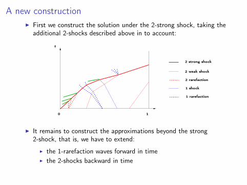
A new constructionI First we construct the solution under the 2-strong shock, taking the

additional 2-shocks described above in to account:

1 rarefaction

10

t

2 strong shock

2 weak shock

2 rarefaction

1 shock

I It remains to construct the approximations beyond the strong2-shock, that is, we have to extend:

I the 1-rarefaction waves forward in timeI the 2-shocks backward in time

I We construct this approximation by using 1− x as the time variable.

2 shock

1 rarefaction

I we have to solve the interactions.

I There are no interactions inside a family because:I rarefaction fronts go forward in timeI shocks go backward in time

I “Side" interactions of fronts of different families can be solved as inLax’s Theorem.

um

1R

1R

2S

2S

˜um

urt

x

ul

I Finally we get an approximation like:

2 shock

x = 0

x = 1

t

1 rarefaction

I It remains then to prove L∞t (BVx) estimates by adapting Glimm’sfunctionals to the situation, and then to use arguments comparableto the ones used for the Cauchy problem. . .

2. Second step: travelling between constant statesI there are three different zones:

D1 := u , 0 < λ1 < λ2,D2 := u , λ1 < 0 < λ2,D3 := u , λ1 < λ2 < 0.

I inside each zone, one can move along (right or left) wave curves,using simple waves.

u2

x

t

u0

u1

u2

u0

u1

I One can move from a zone to another one by using strong shocks

u0

2 shockon the left

3. Third step: reaching the final state

I The idea is to construct a solution by a backward front-trackingalgorithm

I Problem: backward Riemann problem ?

I This problem is ill-posed:

I Existence: Typically, a rarefaction wave cannot be extendedbackward in a way that respects entropy criterions.

I Uniqueness: Even when a solution exists, there is no uniqueness ingeneral.

ur

ul

u1

u2

urul ur ul

I Other problem: characteristic speeds can be close to 0.I The idea is to construct a solution which includes strong shocks:

2 shock

t t

2 shock

t

1 shock 1 shock

0 ≤ λ1 < λ2λ1 < λ2 ≤ 0 λ1 < 0 < λ2

I We manage to have non-zero characteristic speeds “under theshocks”.

I Using the assumptions on u1, we find particular piecewise constantapproximations of u1: at each discontinuity point, we can“approximately” solve the backward Riemann problem using

I either “shock fans”,I either single rarefaction fronts with small amplitude, and with

large distance between them,I either the shocks from the boundary.

x

shock fan

rarefaction frontsingle

Backward interactions

Interactions inside a familyI Shock/shock interactions: do not occur (Lax’s inequalities)I Rarefaction front/shock interactions: do not occur (Lax’s

inequalities+estimates on the sizes of the fronts)I Rarefaction/rarefaction interactions: these are likely, but must be

avoided.

Interactions for different familiesI Weak waves: one can “solve” the interactions, just as in Lax’s

Theorem2R

1R

1S

1S

2R

urul

2R˜um

um

ul

˜um

um

ur

I Strong shock/weak shock interaction: again, one can extend thesolution by a strong shock and a weak shock, satisfying Schochet’sinteraction estimates.

1 shock

1 shock

strong 2 shock

I Strong shock/weak rarefaction interaction: we solve the backwardinteraction in terms of two incoming shocks of the same family (onestrong, one weak)

1 rarefactionstrong 2 shock

weak 2 shockstrong 2 shock

I The main point is to estimate the distance between consecutiverarefaction fronts of the same family in order to prove that beforepossibly meeting, they must

I either leave the domain,

I either be killed by the meeting of a strong shock of the oppositefamily.

I One has to estimate the (backward-in time) focusing of rarefactionwaves.

I This is done by using Glimm & Lax’s estimates on the spreading ofrarefaction waves (forward-in-time).

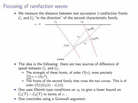
Focusing of rarefaction wavesI We measure the distance between two successive 1-rarefaction frontsC1 and C2 “in the direction” of the second characteristic family.

t = TC1 C2

2-wave

σt

τt

C1(t)

C2(tM )

C2(tm )

I The idea is the following: there are two sources of difference ofspeed between C1 and C2:

I The strength of these fronts, of order O(ν), more precisely∂λ1∂w2

ν +O(ν2).I The fronts of the second family that cross the two curves. This is of

order O(1)|C2(t)− C1(t)|I One uses Oleinik-type conditions on u1 to give a lower bound onC1(T )− C2(T ) in terms of ν. . .

I One concludes using a Gronwall argument.

I We get an approximation like:1

2 strong shock

2 weak shock

1 strong shock

2 rarefaction

1 weak shock

t

0

Conclusion

I The rest of the proof consists in establishing estimates in L∞t (BVx)estimates for these approximations, as in the standard case.

I The idea is to consider modified Glimm functionals V and Q to takeinto account the strong shocks and the construction. . .

I Since the rarefaction fronts never merge, they are always of orderO(ν). Hence we can be sure as for the usual front-trackingalgorithm to obtain an entropy solution in the limit. . .

Open problems

I There is a huge gap between what is known in the framework of C 1

solutions and what is known for entropy solutions.

I For instance, the controllability of the full compressible Eulerequation, with the equation of energy:

∂tρ+ ∂x(ρu) = 0,∂t(ρu) + ∂x(ρu22 + ρθ) = 0,∂t(ρu

2

2 + ρθγ−1 ) + ∂x(ρu

3

2 + γρθuγ−1 ) = 0,

where θ is the temperature, is a completely open problem.

I In some sense the situation is necessarily more complex: in the caseof C 1 solutions, both Euler and Di Perna’s systems are locallycontrollable. . .

Controllability in the vanishing viscosity limit(1D models)

Introduction

I We consider a 1-D conservation law

yt + f (y)x = 0 in [0,T ]× [0, L],

controlled from the boundary.

I Standard controllability problem: given T > 0, y0 and y1 in somefunction space, can we find a solution from y0 at t = 0 to y1 att = T by choosing ad hoc boundary conditions?

I Question. What can be said about the controllability of this systemin a limit of vanishing viscosity?

yt + f (y)x − εyxx = 0 as ε→ 0+?

A motivation

I Boundary control of hyperbolic systems of conservation laws (k ≥ 2)

ut + f (u)x = 0, u : [0,T ]× [0, L]→ RN , f : Rk → Rk ,

in the context of entropy solutions.

I Entropy solutions are weak solutions obtained by vanishing viscosity:

uε → u as ε→ 0+ where uεt + f (uε)x − εuεxx = 0.

Cf. Hopf, Oleinik, Lax, Vol’pert, Kruzhkov, Bianchini-Bressan, etc.

I Question. Is it possible to obtain a uniform control for the viscousequation as ε→ 0+?

I. The problem of null controllability in the vanishingviscosity limit, linear case

I Raised by Coron and Guerrero (2005)I Consider the control system:

yt + Myx − εyxx = 0 in (0,T )× (0, L),

y|x=0 = v(t), y|x=L = 0 in (0,T ),

y|t=0 = y0 in (0, L).

Questions

I Standard null-controllability problem. Given T > 0, is it possible todrive any y0 to 0 at time T? (The answer is well-known andpositive.)

I Uniform controllability problem. Given T > L/|M|, is it possible todo so at a bounded cost as ε→ 0+?

I Is it possible at least for T ≥ CL/|M|? For which value of C?

Results

Theorem (Coron-Guerrero, 2005)If M > 0 and T > 4.3 L/M or if M < 0 and T > 57.2 L/|M|, then thesystem is uniformly controllable in the sense that there are constantsC , κ > 0, such that for any y0 ∈ L2(0, L) and any ε > 0, one can find acontrol v driving the system to 0 at time T , at a cost

‖v‖L2(0,T ) ≤ C exp(−κε

)‖y0‖L2(0,L).

Results, 2

Theorem (Coron-Guerrero, 2005)If M > 0 and T < L/M or if M < 0 and T < 2L/|M|, then the system isnot uniformly controllable in the sense that there exist C , κ > 0, suchthat for any ε > 0, there are initial states y0 ∈ L2(0, L) for which anycontrol v driving the system to 0 at time T satisfies

‖v‖L2(0,T ) ≥ C exp(κε

)‖y0‖L2(0,L).

Conjecture. The times L/M if M > 0 and 2L/|M| if M < 0 areoptimal, that is, the system is uniformly controllable for times T > L/Mif M > 0 and T > 2L/|M| if M < 0.

The problem is still open!

Other references

I Guerrero-Lebeau: N-D transport equation in the vanishing viscositylimit:

yt + M(t, x).∇y − ε∆y = 0.

→ Cost of order O(e−1/ε) if T is large enough and thecharacteristics all meet the control zone, of order O(e1/ε) for Tsmall.

I G.-Guerrero: diffusive-dispersive limits in the linear case

yt −Myx + νyxxx − εyxx = 0,

as ν, ε→ 0+.

Proofs: the approach by real analysis, linear case

I Cf. Coron-Guerrero (see also G.-Guerrero for diffusive-dispersivelimits)

I The standard duality argument (D. Russell, J.-L. Lions, etc.) showsthat if one can prove for the adjoint system

−ϕt + Mϕx − εϕxx = 0 in (0,T )× (0, L),

ϕ(t, 0) = ϕ(t, L) = 0 in (0,T ),

ϕ(T , x) = ϕT (x) in (0, L).

the following observability inequality∫ L

0|ϕ(0, x)|2 dx ≤ K (T0,M, ε)

∫ T

0|ϕx |x=0|2 dt.

then for any y0, one can find controls v1, v2 = 0 that drive thesystem to 0, with

‖v1‖2L2(0,T ) ≤K (T ,M, ε)

ε‖y0‖2L2(0,L).

I One proves a Carleman inequality for the system, à la Fursikov &Imanuvilov. Let β a strictly positive, strictly increasing and concavepolynomial of degree 2. We consider the weight function

exp(−sα) with α(t, x) :=β(x)

t(T − t), s ≥ 0.

Proposition. There exist a constant C > 0 independent of T , ε > 0 and

M ∈ R such that for any ϕT ∈ L2(0, L), one has

s∫ T

0

∫ L

0αe−2sα

(ε2|ϕx |2 + ε2s2α2|ϕ|2

)dx dt

≤ C∫ T

0e−2sα|x=0 |ϕx |x=0|2 dt,

for any s ≥ C (T 2 + T (1 + T |M|))/ε, where ϕ is the correspondingsolution of the adjoint system.

I Idea of proof of this inequality:

I Consider ψ := e−sαϕ, where ϕ is a solution of the adjoint systemLϕ = 0.

I Decompose L(esαψ) = 0 as

L1ψ + L2ψ = L3ψ,

with L1 skew-symmetric, L2 symmetric, L3 corresponding to the“residual terms”.

I Write (with Q0 := (0,T0)× (0, 1))

‖L1ψ‖2L2(Q0) + ‖L2ψ‖2L2(Q0) + 2∫∫

Q0

L1ψ L2ψ dx dt = ‖L3ψ‖2L2(Q0).

I Develop the integral, operate many integration by parts, and absorbseveral terms with the left hand side by taking s large enough.

I Once the Carleman estimate is proven, mix with an energy estimateon ϕ:

‖ϕ(0)‖L2 ≤ ‖ϕ(t)‖L2 ,

to obtain the observability inequality.

I This yields an observability inequality of order

K ∼ expCε

.

I This constant is huge. This is normal, since we did not use thetransport effect.

I The idea is to use a dissipation estimate (here, for the adjointequation) to compensate the size of these constants.

Exponential dissipation estimatesI A close result was obtained by Danchin for the problem of the

vanishing viscosity limit of vortex patches.

I Let us consider some time T1 and times 0 ≤ t1 < t2 ≤ T1.

I One multiplies the adjoint equation with exp(r(M(T1 − t)− x))ϕ,one integrate with respect to x (where r is a positive parameter).

I It is essential here that the function (t, x) 7→ M(T1 − t)− x is asolution of the transport equation.

I After several integration by part, one gets

− ddt

(exp−εr2(T1−t)

∫ L

0expr(M(T1−t)−x)|ϕ(t, x)|2 dx

)≤ 0.

I One integrates with respect to time between t1 and t2, and one gets

∫ L

0|ϕ(t1, x)|2dx ≤ exp

ε(t2 − t1)r2 + (L−M(t2 − t1))r

∫ L

0|ϕ(t2, x)|2dx .

I One optimizes with respect to r to deduce when t2 − t1 ≥ L/M∫ 1

0|ϕ(t1, x)|2dx ≤ κ

∫ 1

0|ϕ(t2, x)|2dx ,

with κ satisfying

κ ≤ exp−c (M(t2 − t1)− L)2

ε(t2 − t1)

,

I If t2 − t1 ≥ K0/M for K0 large enough, this allows to “absorb” theconstant coming from the Carleman inequality.

Carleman

t = 0 t = T1 t = T

Dissipation estimate

II. The problem of null controllability in the vanishingviscosity limit, nonlinear case

I Viscous Burgers equation:

ut + uux − εuxx = 0 in (0,T )× (0, 1), (B)u|t=0 = u0 in (0, 1), (IC)

u|x=0 = v1(t) in (0,T ), u|x=1 = v2(t) in (0,T ). (BC)

I Theorem (G.-Guerrero): There is a constant α0 ≥ 1 such that forany M ∈ R \ 0 there exists ε0 > 0 such that for anyu0 ∈ L∞([0, 1]), any time T > α0/|M| and any ε ∈ (0, ε0) thereexist controls vε1 and vε2 satisfying the following properties:• The solution u of (B)-(IC)-(BC) associated to v1 = vε1 andv2 = vε2 satisfies:

u|t=T = M in (0, 1).

• ‖vε1‖∞ and ‖vε2‖∞ are uniformly bounded for ε ∈ (0, ε0):

∃C > 0 such that ‖vε1‖∞ + ‖vε2‖∞ ≤ C (‖u0‖∞ + |M|).

A recent generalizationTheorem (Léautaud): Consider the control system

ut + f (u)x − εuxx = 0, u(t, 0) = v1(t), u(t, 1) = v2(t),

where the flux function f ∈W 2,∞(R) satisfies f ′′ ≥ 0 a.e. andf ′(u)→ +∞ as u → +∞ (resp. f ′(u)→ −∞ as u → −∞).Then, there exists α0 ≥ 1 and a constant C such that for all R > 0 andall M satisfying

f ′(M) > 0 (resp.f ′(M) < 0),

there exists ε0 > 0 such that for any u0 ∈ L∞ with ‖u0‖∞ ≤ R, any timeT > α0/|f ′(M)| and any ε ∈ (0, ε0) there exist two control functions onthe boundaries satisfying

‖v1‖∞ + ‖v2‖∞ ≤ C (R + |M|),

such that the corresponding solution starting from u0 satisfies

u|t=T = M.

Proof: the approach by real analysis, nonlinear case

Mix the hyperbolic and parabolic approaches:

I Idea coming from the hyperbolic approach: “Destabilize” the systemby sending a viscous travelling wave, followed by a viscousrarefaction wave,

I Use Fursikov and Imanuvilov’s approach to the parabolic system: useCarleman estimates to control the “parabolic part”.

First stepI In a first step, one wants to eliminate the initial conditions.

I One uses travelling waves for (B), that is, solutions of the form

u(t, x) = U(x − ctε

) t ∈ R+, x ∈ R, with

u(t, x) −→ U± as x → ±∞,ux(t, x) −→ 0 as x → ±∞,

I “Complete” u0 in [0, 1] with an appropriate travelling wave onR \ [0, 1]: (here N ‖u0‖∞)

u0

N

0 1

I Wait some time T1 (of order O(1/N)), until the state in [0, 1] issufficiently close to N.

I Use the “parabolic” control to drive the state u(T1) to exactly N intime T ∗ (of order O(1/N)).

I As before, this is done by proving an observability inequality for theadjoint of the linearized equation

−ϕt − εϕxx − z(t, x)ϕx = 0 in (0,T ∗)× (0, 1),

ϕ|x=0 = 0, ϕ|x=1 = 0 in (0,T ∗),

ϕ|t=T∗ = ϕ0 in (0, 1),

‖ϕ|t=0‖2L2(0,1) ≤ K (T ∗, ε)2∫ T∗

0(|ϕx|x=0|2 + |ϕx|x=1|2) dt (OI)

I If (OI) is proved, then one can find controls for the linearizedequation, and then perform a fixed-point argument.

I The main fact is the following: the controls obtained above satisfythe estimate :

‖vε1‖+ ‖vε2‖ ≤ K (T ∗, ε)‖u(T1)− N‖L2(0,1).

I Of course, the observability constant K (T ∗, ε) blows up as ε→ 0+.Looking carefully to the Carleman estimate that allows to prove(OI), one can show that

K (T ∗, ε) = O(exp(C1

ε)).

I But this is compensated by the fact that as ε→ 0+, the travellingwaves approach a shock wave (composed of two constant states), sothat one can show again that

‖u(T1)− N‖L2(0,1) = O(exp(−C2

ε)),

with C2 > C1 if one lets the travelling wave pass during a sufficientlylong time. (Uses maximum principle!)

Second step

I Here one completes the state N in [0, 1] with N on the right and thetarget M on the left.

M

10

N

I This yields a viscous rarefaction wave.

I The same type of reasoning as in the previous steps yieldsappropriate controls.

III. Approaching the problem by complex analysisI One can try to approach Coron and Guerrero’s problem (the

vanishing viscosity limit for the transport equation), by suitablyemploying complex-analytical arguments.

I This allows to improve the time constants in the Coron-Guerrerotheorem.

Theorem (G., 2009)The control system:

yt + Myx − εyxx = 0 in (0,T )× (0, L),

y|x=0 = v(t), y|x=L = 0 in (0,T ),

y|t=0 = y0 in (0, L),

is still uniformly controllable if M > 0 and T > 4.2L/M or if M < 0 andT > 6.1L/|M|.

RemarkCoron and Guerrero gave T > 4.3L/M if M > 0 and T > 57.2L/|M| ifM < 0. The main point is that the proof is of completely differentnature...

The approach by complex analysisI The proof uses the method of moments, cf. Fattorini-Russell (1971).I It is also connected to the study of the cost of the control of

parabolic systems for small times, cf.I Seidman, Seidman-Gowda, Seidman-Avdonin-Ivanov,I Fernández-Cara-Zuazua,I Miller,I Tenenbaum-Tucsnak,I ...

I Of course, by a time-scaling argument, it is essentially equivalent tocontrol

ut −∆u = 0,

during the time interval [0, εT ], and to control

ut − ε∆u = 0,

during the time interval [0,T ].

I One still wants to prove an observability inequality of the type

‖ϕ(0, ·)‖L2(0,L) ≤ K exp(− κ

ε

)‖∂xϕ(·, 0)‖L2(0,T ),

for the adjoint equation ϕt + Mϕx + εϕxx = 0 in (0,T )× (0, L),ϕ = 0 on (0,T )× 0, L,ϕ(T , ·) = ϕT in (0, L).

I One can easily diagonalize the operator

P := −M∂x − ε∂2xx ,

by noticing that

∂2xx(e

Mx2ε u) = e

Mx2ε

(∂2

xxu +Mε∂xu +

M2

4ε2u),

I Hence the operator −M∂x − ε∂2xx is diagonalizable in L2(0, L), with

eigenvectors

ek(x) :=√2 exp

(− Mx

2ε

)sin(kπx

L

). (2)

for k ∈ N \ 0 and corresponding eigenvalues

λk := εk2π2

L2 +M2

4ε, (3)

the family ek , k ∈ N \ 0 being a Hilbert basis of L2(0, L) for theL2((0, L); exp(Mx

ε ) dx) scalar product.

I Consider a solution ϕ of the adjoint system, where

ϕT (x) =N∑

k=1

ckek(x).

I We deduce easily

∂xϕ(t, 0) =N∑

k=1

ck√2kπL

exp(−λk(T − t)).

and

ϕ(0, x) =N∑

k=1

ck exp(−λkT )ek(x).

I Imagine that we have a family ψk which is bi-orthogonal to thefamily fk : t 7→ exp(−λk(T − t)) in L2(0,T ):

〈fj , ψk〉L2(0,T ) = δj,k ,

then one deduces that

√2kπ

Lck =

∫ T

0(∂xϕ)(t, 0)ψk(t) dt.

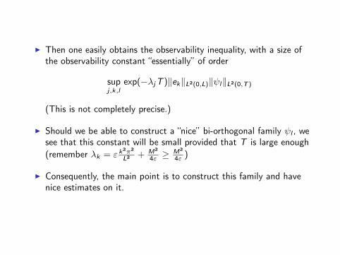
I Then one easily obtains the observability inequality, with a size ofthe observability constant “essentially” of order

supj,k,l

exp(−λjT )‖ek‖L2(0,L)‖ψl‖L2(0,T )

(This is not completely precise.)

I Should we be able to construct a “nice” bi-orthogonal family ψl , wesee that this constant will be small provided that T is large enough(remember λk = ε k2π2

L2 + M2

4ε ≥M2

4ε )

I Consequently, the main point is to construct this family and havenice estimates on it.

Construction of the bi-orthogonal familyI Imagine that you are given an entire function J ∈ H(C), of

exponential type T/2: for some constant C > 0, one has

|J(z)| ≤ C exp(T |z |/2) for all z ∈ C,

having simple zeros at the points −iλk and whose restriction to R isin L2.

I Then one defines

Jk(z) :=J(z)

J ′(−iλk)(z + iλk),

which is still an entire function of exponential type T/2, is still in L2

on R, and it satisfiesJk(−iλj) = δjk .

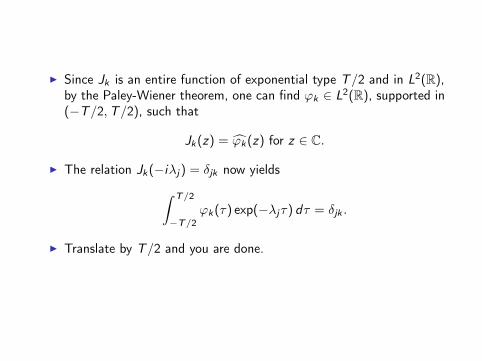
I Since Jk is an entire function of exponential type T/2 and in L2(R),by the Paley-Wiener theorem, one can find ϕk ∈ L2(R), supported in(−T/2,T/2), such that

Jk(z) = ϕk(z) for z ∈ C.

I The relation Jk(−iλj) = δjk now yields∫ T/2

−T/2ϕk(τ) exp(−λjτ) dτ = δjk .

I Translate by T/2 and you are done.

I Hence the core of the proof is to construct an entire function J, ofexponential type T/2, having simple zeros at −iλk , whose restrictionto R belongs to L2, and yielding the best possible estimates.

I An entire function having the k2, k ∈ N \ 0 as its simple zeros isthe following Weierstrass product:

∞∏k=1

(1− z

k2

)=

sin(π√z)

π√z

,

which is an entire function (despite the square roots).I Now a function having simple zeros exactly at −iλk , k ∈ N \ 0

by

Φ(z) =

sin(

L√ε

√iz − M2

4ε

)L√ε

√iz − M2

4ε

. (4)

I It is elementary to see that Φ is of exponential type, and evensatisfies

|Φ(z)| ≤ C (M, ε) exp(L√2ε

√|z |) as |z | → +∞. (5)

I But precisely because of this “sub”-exponential estimate, thePhragmen-Lindelöf theorem (or direct computations) proves thatthis function cannot be bounded on the real line.

I Hence, the idea is to find another entire function F ∈ H(C), called amultiplier, such that

I the function F (z)Φ(z) now suitably behaves on the real line,I it is of exponential type T/2.

Such a technique can be traced back to R. Paley and N. Wienerthemselves.

The Beurling-Malliavin multiplierI We use a construction of a multiplier due to Beurling and Malliavin

(1961).I Introduce

s(t) =T2π

t − Lπ√2ε

√t.

We notice that s is increasing for t larger than

A :=12ε

(LT

)2

. (6)

I Using that∫ ∞0

log∣∣∣∣1− x2

t2

∣∣∣∣ dtγ = |x |γπ cot πγ2

for 0 < γ < 2,

we see that ∫ ∞0

log∣∣∣∣1− x2

t2

∣∣∣∣ ds(t) = − L√2ε

√|x |.

I We introduce

B := 4A =2ε

(LT

)2

, (7)

which satisfies s(B) = 0.I Now one defines ν as the restriction of the measure ds(t) to the

interval [B,+∞). Let us underline that this measure is positive(since B ≥ A).

I Next we introduce for z ∈ C:

U(z) :=

∫ ∞0

log∣∣∣∣1− z2

t2

∣∣∣∣ dν(t) =

∫ ∞B

log∣∣∣∣1− z2

t2

∣∣∣∣ ds(t), (8)

and for z ∈ C \ R

g(z) :=

∫ ∞0

log(1− z2

t2

)dν(t) =

∫ ∞B

log(1− z2

t2

)ds(t). (9)

I By “atomizing” the measure dν in the above integral, we can define

U(z) :=

∫ ∞0

log∣∣∣∣1− z2

t2

∣∣∣∣ d [ν(t)], (10)

where [ · ] denotes the integer part and where

ν(t) =

∫ t

0dν. (11)

In the same way as previously we introduce

h(z) :=

∫ ∞0

log(1− z2

t2

)d [ν](t). (12)

I Of course,

U(z) = Re(g(z)) and U(z) = Re(h(z)).

Now exp(h(z)) is an entire function. Indeed, calling µk , k ∈ Nthe discrete set in R consisting of the discontinuities of the functiont 7→ [ν(t)], we have

exp(h(z)) =∏k∈N

(1− z2

µ2k

). (13)

I Finally, the multiplier which we will use is the following:

F (z) := exp(h(z − i)).

I The rest of the proof consists in proving that F (z)Φ(z) is ofexponential type T/2, and to give estimates on x 7→ F (x)Φ(x) on Rand on F (−iλk), so that we have the correct estimates on

Jk(z) =F (z)Φ(z)

F (−iλk)Φ′(−iλk)(z + iλk).

I 1. Estimates on the real line.

LemmaFor x ∈ R, one has

U(x) ≤ − L√2ε

√|x |+ C1aB, (14)

where C1 is the following positive (and finite) constant

C1 := −minx∈R

∫ 1

0log∣∣∣∣1− x2

t2

∣∣∣∣ d(t −√t) ' 2.34 < 2.35. (15)

Lemma (Koosis)We have for z = x + iy ∈ C:∫ ∞

0log∣∣∣∣1− z2

t2

∣∣∣∣ d([ν](t)−ν(t)) ≤ log(max(|x |, |y |)

2|y |+

|y |2max(|x |, |y |)

).

(16)

I Using the fact that U is a harmonic function on the upper plane,hence admits an integral representation, one can compare U(x − i)and U(x), and finally get the following estimate on the multiplier:

∀x ∈ R, U(x − i) ≤ − L√2ε

√|x |+ aBC1 + log+(|x |) +

T2.

I 2. Estimates on the imaginary axis.

LemmaFor all y ∈ R one has∫ ∞

Blog(1 +

y2

t2

)d [s] ≥

∫ ∞B

log(1 +

y2

t2

)ds − log

(1 +

y2

B2

). (17)

LemmaOne has ∫ B

0log∣∣∣∣1 +

y2

t2

∣∣∣∣ ds = aBG( yB

). (18)

where

G (y) :=

∫ 1

0log∣∣∣∣1 +

y2

t2

∣∣∣∣ d(t −√t)

is a bounded function.

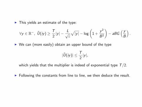
I This yields an estimate of the type:

∀y ∈ R−, U(iy) ≥ T2|y | − L√

ε

√|y | − log

(1 +

y2

B2

)− aBG

( yB

).

I We can (more easily) obtain an upper bound of the type

|U(iy)| ≤ T2|y |,

which yields that the multiplier is indeed of exponential type T/2.

I Following the constants from line to line, we then deduce the result.

Open problems

I The Coron-Guerrero conjecture is still open!

I When dispersion is present, so is the case of negative M. . .

I Can one estimate the time of uniform controllability for variable M?

I Can one treat the high frequencies and the low frequenciesdifferently? (We are not optimal for the high frequencies; perhapswe could use the Lebeau-Robbiano-Zuazua spectral inequality forthe low frequencies?)

I What can be said about nonlinear equations?

I Can one consider the case of systems? (Long horizon quest: controlthe compressible Navier-Stokes with small viscosity...)