Assignments for Bradie Fall 2016 ALL

Read pages 1-16; Note there is a typo (error) in Equation 3 page 3; it should have the last term as

ktce , the minus sign is missing.

For 2, 3, 4, Use your calculator and record details of the steps. (No MATLAB m-file required.) For the airplane problem show all your work. For 15 construct an algorithm like that for the Trapezoidal Rule on P. 13. Then use MATLAB routine bradie_sec1_1_num15.m. Use command bradie_sec1_1_num15(Nmax, 5E-3) where you specify a value for Nmax. In MATLAB type help bradie_sec1_1_num15 for information. +++++++++++++++++++++++++++++++++++++++++++++++++++++++++++++++++++++++++ Read pages 20-27; there are important concepts and terminology in this section.

For 2a, b use Taylor series expression with a few terms. For 3 determine a table of values for x = 1. 0.1, 0.01, 0.001, keeping as many digits as your calculator permits. (Just do the numerical work.) For 6 use the contents of the sentence below the definition that is on Page 23. Exercises 13-15 are important for later theoretical work. You are responsible for reading, understanding the steps in the proofs, and answering the questions attached to steps in the proofs of these exercises. The proofs are available on the course website. +++++++++++++++++++++++++++++++++++++++++++++++++++++++++++++++++++++++++++ Read Pages 30-39; Make sure you know the definition of roundoff error.

For #1 use your calculator and set up table with headings like the following.

For #6a, b just determine the number of significant digits in base 10.

Some problems require the use of a calculator, others need MATLAB. Solutions

are to be submitted on paper, and usually require two parts: (a) a description of

the underlying theory; and (b) code segments, printouts of program outputs, plots,

and whatever it required to convince the grader that you have understood the

theory and addressed all practical challenges appropriately. All things must be

clearly labeled with your name and the problem number or statement. Hand

written work must include the steps for solution presented in a neat orderly

fashion and in a fairly large size. ALL SOLUTIONS ARE TO INCLUDE ALL STEPS

USED TO SOLVE THE PROBLEM.

Exercises for Section 1.3: #1a,b,e, 6a,b, 7, 15a, b, 16, 18 Math on Computer

Exercises for Section 1.1: #2, 3, 4, 6, 15 Algorithms and airplane landing problem (available no my web site)

Exercises for Section 1.2: #1, 2a,b, 3, 6, 13, 14, 15, 16 Convergence

For #7 you are told that the values have been rounded to the digits shown. So here you must determine an appropriate interval that contains the value of a parameter. For example in part (a) P = 0.750 atm, thus we must consider a range of values ±0.0005 from the given value 0.7495 < P < 0.7505. Do this for each parameter, then set up an interval that contains the desired expression. For #16 there is a description for solving first order linear DEs on my website. ++++++++++++++++++++++++++++++++++++++++++++++++++++++++++++++++++++++++++++ Read Pages 42-50; In particular Example 1.11 reveals how floating point arithmetic impact solving linear system of equations

Graphical Exercise: The polynomial p(x) = (x – 1)6 can be expanded in MATLAB. Use the code syms x,p=(x-1)^6;;expand(p) . We want to plot the expansion over increasingly smaller intervals around x = 1. Use the script file zoomplot. (Just type zoomplot.) Six subplots will be generated. The x-axis will appear as a horizontal line in each plot. Write a description of the plots as the interval becomes smaller. Is the behavior depicted in the graphs what you would expect when graphing p(x) = (x – 1)6 ? Explain. What accounts for the behavior in the graphs?

For #1 follow the ideas in the example below. For #5 in order to see where 3

2

6

xx use Taylor series

for xe and cos(x) ; the steps for this are not required.

For #12 consider using trig identities, properties of logs, etc.

Example: 1c; compute the 4-digit rounding value of πln(2) + 10 cos(22°).

Step 1. Find the “float values of each value: fl(π) = fl(3.141592654) = 3.142 fl(ln(2)) = fl(0.6931471806) = 0.6931

fl( 10 ) = fl(3.16227766) = 3.162

fl(cos(22°) = fl(0.9271838546) = 0.9272 Step 2. Compute the products in the floating point system. fl(3.142 × 0.6931) = fl(2.1777202) = 2.178 fl(3.162 ×0.9272) = fl(2.9318064) = 2.932 Step 3. Compute the sum in floating point system. fl(2.1278 + 2.932) = fl(5.110) = 5.110 ++++++++++++++++++++++++++++++++++++++++++++++++++++++++++++++++++++++++++++ Read Pages 54-68.

For #1 and #2 do the computations by hand/calculator showing your steps to 5 decimal places. Record values in a table like Left End Point XL Right End Point XR Midpoints XM Function Value at XM Indicate the signs of the function values at the ends of the intervals. For #13, 15, 18 use Bisection Method software. +++++++++++++++++++++++++++++++++++++++++++++++++++++++++++++++++++++++++++

Exercises for Section 1.4: #1a,b, 2, 5, 7a, 12a,c,d Floating Point

Exercises for Section 2.1: #1a,b, 2, 13, 15, 18 Bisection

Read Pages 71-78.

For #1a, b do the computations by hand/calculator showing your steps to 5 decimal places. Record values in a table like the following. The sequence of x-intercepts p1, p2, p3 is what is requested. The initial interval in “technically” not counted as members of the sequence of approximations. So you need to compute 3 x-intercepts and the next interval containing the root. XL XR pn = Xinter f(Xinter) For #4 you are asked to perform 5 iterations. In order to use the error approximation you need 3 x-intercept values. That means you compute p1, p2, and p3 before using the error estimate and then p4 and p5. Show your steps from hand/calculator computations carrying at least 5 decimal places and display the results in a table in the following form: n pn |pn – p| Error Estimate

++++++++++++++++++++++++++++++++++++++++++++++++++++++++++++++++++++++++++++ Read Pages 81 – 93

For #1a, recall that pn – pn-1 = g(pn-1) – g(pn-2) and use the Mean Value Theorem. For part b, recall that for linearly convergent fixed point scheme the asymptotic error constant is λ = g'(p), thus en ≈ g'(p) en-1 and that en = p – pn. For #6, you can use software to compute the seven approximations, but then you need to compute the exact error for p1 through p7 as well as use formulas in Equations (1) and (2) to estimate the per step error. For #8 the Theorem on Page 91 is useful.

For #11 you will need MATLAB fixed point software. Assume part (a) is true and 1/2k 2 e .

For #14 you will need fixed point software +++++++++++++++++++++++++++++++++++++++++++++++++++++++++++++++++++++++++++++ Read Pages 95 – 107

For #1a, c do computations by hand/calculator displaying steps and all work; p0 = 0. For #5 Use software in MATLAB to get the five iterations, p1 thru p5 with p0 = 3. For #10, use software in Matlab. For (b) use p0 = 3.5.

These are to be done using YOUR code from lab for method of false position. For #11a and 13 use Method of False Position software. For #12 use Equation (7) to help infer behavior.

Exercises for Section 2.2: #1a,b, 4, 11a, 12, 13 False Position

Exercises for Section 2.3: #1, 6, 8, 11b ,c, 14 Fixed Point

Exercises for Sec 2.4: #1a, c, 5, 10, 11 Newton

For #11, use software in Matlab. Determine (estimate) the asymptotic error constant. +++++++++++++++++++++++++++++++++++++++++++++++++++++++++++++++++++++++++++++ Read Pages 107 – 111

For #1a do computations by hand/calculator displaying steps and all work; p0 = 0, p1 = 1. For #7 use MATLAB secant software to get the five iterations, p2 thru p8 with p0 = 2, p1 = 3. For #11 use MATLAB secant software. For #20 replace the $20,000 by $25,000. Figure out why I want you to use this change. Use software secant for the computations. +++++++++++++++++++++++++++++++++++++++++++++++++++++++++++++++++++++++++++++ Read Pages 114 – 122

For #3 use Matlab files aitken .m and errorcomp.m to assist with the computations. For #6 use Steffensen’s method; part can be done using atiken.m . Explain how you can conclude that quadratic convergence is achieved. +++++++++++++++++++++++++++++++++++++++++++++++++++++++++++++++++++++++++++

Exercises for Sec 2.5: #1a 3, 7, 11a, 20 Secant

Exercises for Sec 2.6: #1, 2, 3, 6, 12 Accelerating Convergence

Assignments for Bradie Fall 2016 for Chapter 3

Read Pages 149 – 157

For #1& #2, do by hand using exact arithmetic (fractions as needed) via Gaussian Elimination. Here you must identify the pivots, show the row operations, show the equivalent upper triangular system, and the back substitution steps. Important note: There is a typo in my book for the second equation in #10. The right side should be 3.67 NOT 7.23. For #10 & #11.Here you can use Matlab programs reduce.m & bksub.m. You must print out the upper triangular form and the result of back substitution. For #16. Here you can use Matlab programs reduce.m & bksub.m. SHOW THE ORIGINAL MATRIX you construct. You must print out the upper triangular form and the result of back substitution. +++++++++++++++++++++++++++++++++++++++++++++++++++++++++++++++++++++++++++ Read Pages 160 – 167

You need to have UPGRADED the course collection of m-files to 3043mfilesVERSION2. This was emailed to you. It is also available on my website. When you set the path for this new version click the button ADD with Subfolders button. For #1a,b #2, #3 use hand calculations. For #13 use Matlab program genopiv.m to show that the vector x is the solution. (You must set the number of digits to use to 4.) Print out the upper triangular matrix that results from using genopiv.) Use the result of genopiv in routine bksub to verify x is a solution. Print out the result. Next solve the

Some problems require the use of a calculator, others need MATLAB. Solutions

are to be submitted on paper, and usually require two parts: (a) a description of

the underlying theory; and (b) code segments, printouts of program outputs, plots,

and whatever it required to convince the grader that you have understood the

theory and addressed all practical challenges appropriately. All things must be

clearly labeled with your name and the problem number or statement. Hand

written work must include the steps for solution presented in a neat orderly

fashion and in a fairly large size. ALL SOLUTIONS ARE TO INCLUDE ALL STEPS

USED TO SOLVE THE PROBLEM.

Exercises for Sec 3.1: #1, 2, 10a, b, 11a,c , 16 Gaussian Elimination

Exercises for Sec 3.2: #1a, b Parts (i), (ii),(iii), 2, 3, 13, 14 (i), (ii) Pivoting Strategies

system using Matlab’s \ (backslash) command to get a very good solution. Compare the very good solution to the vector x by computing the relative error. For #14 (i) use the Matlab routine genopiv.m (You must set the number of digits to use to 3.) Print out the upper triangular matrix that results from using genopiv.), (ii) use the Matlab routine geppivot.m . Print out the upper triangular matrix that results from using geppivot.) Compare the results by writing a sentence of explanation. (Use geppivot in the form geppivot(A).) ++++++++++++++++++++++++++++++++++++++++++++++++++++++++++++++++++++++++++++

Read pages 191 – 201; you can skip the subsection on the Inverse Power Method pp. 200-201

For # 4a, b, #5c, #6a, #7, #10a use hand calculations. For #H3 and H4 you can use Matlab routine lufact.m . ++++++++++++++++++++++++++++++++++++++++++++++++++++++++++++++++++++++++ Read Pages 249-top of 252

1. Use Newton's method for systems to obtain (by primarily using a calculator; you can use MATLAB backslash command to solve linear systems encountered) three new estimates of a solution starting with initial guess (x0, y0) = (0,2) to the system f(x,y) = 5x2 + y2 - 5 = 0 g(x,y) =y2 - 2y - x + 0.25 = 0

Explicitly show the Jacobian, x , y , and the updated solution approximation for each step and carry at least 6 decimals in your calculations.

Exercises for Sec 3.10 Nonlinear Systems; Newton’s Method

Exercises for Sec 3.5 #3, #4a, b, #5c, #6a, #7, #10a, and following exercises H1 – H4.

H1. Let 2 1

6 3A

. Determine 1 0

and 1 0

a bL U

s c

so that A L U using only matrix

multiplication.

H2. Let

4 1 0

1 4 1

0 1 4

A

. Determine

0 0 1

0 and 0 1

0 0 1

a g h

L b c U j

d e f

so that A L U using only

matrix multiplication.

H3. Find an LU-factorization of

1 2 3

2 1 1

5 0 2

A

. Use partial pivoting and the pivot vector device.

Express L and U in pseudo triangular form; see Example 4. Or, use Matlab routine lufact.m and then figure out how to form L and U in standard form. H4. Let A = 13 39 2 57 28 -4 -12 0 -19 -9 3 0 - 9 2 1 6 17 9 5 7 19 42 -17 107 44 Use lufact.m and then figure out how to form L and U; Write them in standard form for the type of matrix. Then form the permutation matrix P.

2. Use Newton's method for systems to obtain (by primarily using a calculator; you can use MATLAB backslash command to solve linear systems encountered) three new estimates of a solution starting with initial guess (x0, y0) = (3.5,3) to the system f(x,y) = x2 - y2 - 4 = 0 g(x,y) =y2 - 2y - x + 0.25 = 0

Explicitly show the Jacobian, x , y , and the updated solution approximation for each step and carry at least 6 decimals in your calculations.

3. For the nonlinear system

2 21 2 2

21 2

x x 2x 0

2x x 6 0

determine the number of solutions. Hint: a picture can

help. Show your work to determine your answer. 4. What does Newton’s Method for nonlinear systems reduce to for the linear system Ax = b where A is a nonsingular matrix. Display the multivariate function F(x), the Jacobian of the system and write the Newton algorithm in the form

for the case n = 0.

Hint: Let j 1 2 n j1 1 j2 2 jn n jf x , x , ...,x a x a x ... a x b , determine the multivariate function F(x), and

determine the Jacobian. Ref: B&F 8 +++++++++++++++++++++++++++++++++++++++++++++++++++++++++++++++++++++++++++ Read My Notes for Material on Iterative Methods (My notation and coverage varies from that in the text in Section 3.8. The text covers more material than I want to discuss at this time.)

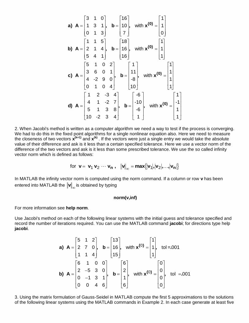
When an example is cited below it appears in my notes. 1. Use Jacobi's method as in illustrated in Example 1 to approximate the solution of each of the following linear systems. (You can use the MATLAB commands as in Example 1.) In each case generate at least five approximations showing the results in a table. Make a conjecture as to whether the process appears to be converging or not.

Exercise Number

SET A Exercise Parts

SET B Exercise Parts

#1 a, c b, d

#2 a b

#3 a, c b, d

#4 The parts assigned for #1, #2, #3

The parts assigned for #1, #2, #3

#5 all all

#6 all all

#7 all all

#8 all

#9 all

Last two ID DIGITS

Do the exercises listed below.

00-19 Set A

20-29 Set B

30-39 Set A

40-49 Set B

50-59 Set A

60-69 Set B

70-79 Set A

80-89 Set B

90-99 Set A

a A b x

b) A b x

c A b x

) , ,

, ,

) , ,

( )

( )

(

3 1 0

1 3 1

0 1 3

16

10

7

with

1

1

0

1 1 5

2 1 4

5 4 1

18

16

16

with

1

1

1

5 1 0 2

3 6 0 1

4 -2 9 0

0 1 0 4

1

11

-8

10

with

L

NMMM

O

QPPP

L

NMMM

O

QPPP

L

NMMM

O

QPPP

L

NMMM

O

QPPP

L

NMMM

O

QPPP

L

NMMM

O

QPPP

L

N

MMMM

O

Q

PPPP

L

N

MMMM

O

Q

PPPP

0

0

0

0

)

( )) , ,

L

N

MMMM

O

Q

PPPP

L

N

MMMM

O

Q

PPPP

L

N

MMMM

O

Q

PPPP

L

N

MMMM

O

Q

PPPP

1

1

1

1

1 2 -3 4

4 1 -2 7

5 1 3 8

10 -2 3 4

-6

-10

-6

1

with

1

-1

1

1

d A b x

2. When Jacobi's method is written as a computer algorithm we need a way to test if the process is converging. We had to do this in the fixed point algorithms for a single nonlinear equation also. Here we need to measure the closeness of two vectors x(k+1) and x(k) . If the vectors were just a single entry we would take the absolute value of their difference and ask is it less than a certain specified tolerance. Here we use a vector norm of the difference of the two vectors and ask is it less than some prescribed tolerance. We use the so called infinity vector norm which is defined as follows:

for v v v v v v v vn n 1 2 1 2 , max , , ,m r

In MATLAB the infinity vector norm is computed using the norm command. If a column or row v has been

entered into MATLAB the v

is obtained by typing

norm(v,inf)

For more information see help norm.

Use Jacobi's method on each of the following linear systems with the initial guess and tolerance specified and record the number of iterations required. You can use the MATLAB command jacobi; for directions type help jacobi.

a A b x

b) A b x

) , , , .

, , , .

( )

( )

with tol =

with tol

L

NMMM

O

QPPP

L

NMMM

O

QPPP

L

NMMM

O

QPPP

L

N

MMMM

O

Q

PPPP

L

N

MMMM

O

Q

PPPP

L

N

MMMM

O

Q

PPPP

5 1 2

2 7 0

1 1 4

13

16

15

1

1

1

001

6 1 0 0

2 5 3 0

0 1 3 1

0 0 4 6

6

2

1

6

0

0

0

0

001

0

0

3. Using the matrix formulation of Gauss-Seidel in MATLAB compute the first 5 approximations to the solutions of the following linear systems using the MATLAB commands in Example 2. In each case generate at least five

approximations showing the results in a table. Make a conjecture as to whether the process appears to be converging or not.

a A b x

b) A b x

c A b

) , ,

, ,

) , ,

( )

( )

2 1 0

1 2 1

0 1 2

0

4

4

with

1

1

1

1 1 5

4 1 0

5 0 2

6

10

17

with

1

1

1

5 1 0 2

3 6 0 1

4 -2 9 0

0 1 0 4

1

11

-8

10

L

NMMM

O

QPPP

L

NMMM

O

QPPP

L

NMMM

O

QPPP

L

NMMM

O

QPPP

L

NMMM

O

QPPP

L

NMMM

O

QPPP

L

N

MMMM

O

Q

PPPP

L

N

MMMM

O

Q

PPPP

0

0

with

1

1

1

1

1 2 -3 4

4 1 -2 7

5 1 3 8

10 -2 3 4

-6

-10

-6

1

with

1

-1

1

1

x

d A b x

( )

( )) , ,

0

0

L

N

MMMM

O

Q

PPPP

L

N

MMMM

O

Q

PPPP

L

N

MMMM

O

Q

PPPP

L

N

MMMM

O

Q

PPPP

4. For each of the coefficient matrices in Exercises 1 - 3, determine the eigenvalues of the Jacobi iteration matrix MJ and the Gauss-Seidel iteration matrix MGS. In MATLAB eigenvalues can be computed using the eig command. Use help eig to get information about this command.

5. Given the linear system Ax = b, where

A b

L

N

MMMM

O

Q

PPPP

L

N

MMMM

O

Q

PPPP

4 1 1 0

1 4 0 1

1 0 4 1

0 1 1 4

1

2

0

1

,

a) Starting with an initial guess of x(0) = [1 1 1 1]' compute the first 3 approximations using Jacobi's method. Record the approximations using format short e in MATLAB. b) Repeat part a using Gauss-Seidel. c) Use Atiken acceleration on the 3 vectors obtained in part a to obtain an "improved" approximation. d) Compute the true solution x of this system and compute the infinity norm of (x - last vector) for each of parts a, b, c. 6. The rate of convergence of an iterative method with iteration matrix M is measured by the spectral radius of

M. The spectral radius of a matrix M is denoted (M) and is defined to the maximum of the absolute values of the eigenvalues of M. Determine the rate of convergence for both Jacobi and Gauss-Seidel for the matrix in Exercise 5. Which is faster? Why? How much faster? 7. For each of the following matrices determine which of the methods Jacobi or Gauss-Seidel converge.

a) b) A A

L

NMMM

O

QPPP

L

NMMM

O

QPPP

2 1 1

2 2 2

1 1 2

1 2 2

1 1 1

2 2 1

8. In MATLAB there is a routine called seidel that implements the Gauss-Seidel method based on certain input. Use help seidel to determine how to use this routine. Use routine seidel initial guess x(0) = [0 0 0 0]' and a tolerance of 1.e-5 solve the linear system Ax = b where

A b

L

N

MMMM

O

Q

PPPP

L

N

MMMM

O

Q

PPPP

3 5 47 20

11 16 17 10

56 22 11 18

17 66 12 7

18

26

34

82

,

It is known that this system has a unique solution. Find it using seidel.

9. In MATLAB there is a routine called seidel that implements the Gauss-Seidel method based on certain input. Use help seidel to determine how to use this routine. Use routine seidel initial guess x(0) = [0 0 0 0]' and a tolerance of 1.e-5 solve the linear system Ax = b where

A b

L

N

MMMM

O

Q

PPPP

L

N

MMMM

O

Q

PPPP

2 4 10 20

1 2 6 2

1 8 2 3

10 2 3 4

82

7

14

4

,

It is known that this system has a unique solution. Find it using seidel. 10. In MATLAB there is a routine called seidel that implements the Gauss-Seidel method based on certain input. Use help seidel to determine how to use this routine. Use routine seidel initial guess x(0) = [0 0 0 0]' and a tolerance of 1.e-5 solve the linear system Ax = b where

A b

L

N

MMMM

O

Q

PPPP

L

N

MMMM

O

Q

PPPP

4 8 2 3

12 2 14 0

1 5 9 1

2 41 7 3

12

22

-19

-47

,

It is known that this system has a unique solution. Find it using seidel.

++++++++++++++++++++++++++++++++++++++++++++++++++++++++++++++++++++++++++++++++++

Assignments for Bradie Fall 2016 for Chapter 5 Assignment sheet for Sections 5.1, 5.3, 5.5, 5.6, 5.7, 5.8 Read Pages 341 - 349

For #1 use MATLAB to draw the graphs. For #4 do part (d) carefully. For #13 use MATLAB routine pinterp; capture the formula and graph to include with your answer to the question. For #14 part (b) use MATLAB routine pinterp capture the formula and graph to include with your answer to part (c). ++++++++++++++++++++++++++++++++++++++++++++++++++++++++++++++++++ Read Pages 363 – 369

For #3 and #6 do the calculations by hand; show the work. For #7 construct the divided difference table by hand; do not compute the values of any logarithms. For #15 use MATLAB routines divdiff and divpoly; include print outs from MATALB.

California Problem

Consider the following population data for the state of California.

Year 1940 1950 1960 1970 1980 1990

Population in Millions

6.9 10.5 15.7 19.9 23.6 29.7

Table 1. We are to build an interpolation polynomial model to this data. To simplify the values involved and also possibly to aid in the prevention of roundoff error we 'rescale' the data as follows.

Year 40 50 60 70 80 90

Population in Millions

6.9 10.5 15.7 19.9 23.6 29.7

Table 2.

Enter the data in Table 2, into MATLAB. Call the years x and the populations y. Use routine divpoly in MATLAB do the following. a) The population in 1930 was about 5.7 million. Evaluate the interpolation polynomial to the data in Table 2 at x = 30. Compute the absolute and relative error in the value obtained from the evaluation of the interpolant. b) Use divpoly as in part a, but predict the populations in 1985, 2000, and 2010. Do these values seem reasonable? Explain. c) Use routine pinterp with the data in Table 2 and sketch the interpolant over 1900 to 2010 by setting the minimum value of x to 0 and the maximum to 110. Print out the graph and annotate it to

explain your answers to parts a and b. (Generate the sketch with y-coordinates 0.) DD-Table Problem

Exercises for Section 5.1 Lagrange Interpolation #1, #4, #7, #13, #14

Exercises for Section 5.3 Divided Difference Form of Interpolation #3, #6, #7, #10, #11, #15, California

Problem, DD-Table Problem

Given the following divided difference table.

0th DD 1st DD 2nd DD 3rd DD 4th DD

4 a

f

7 b m

g r

9 c n t

h s

10 d p

k

12 e

(a) Write an expression for the interpolant that goes through the set of ordered pairs {(4,a), (7,b), (9, c)}. (b) Write an expression for the interpolant that goes through the set of ordered pairs { (7,b), (9, c), (10, d), (12, e)}. (c) The point (15, w) is to be added to the table. Write and expression for the interpolant through the ordered pairs {(12, e), (15, w)}. ++++++++++++++++++++++++++++++++++++++++++++++++++++++++++++++++++++++++

Do the following Exercises. #1. Given a curve, collect a sample of points, generate the corresponding polynomial interpolant, and then compare the graph of the interpolant with the original curve. Since a limited sample of points will be permitted it is important to take the sample from portions of the curve that in some sense control or significantly affect its shape. Such a strategy can aid the model constructed by the interpolant, but is not a guarantee that the model produced will match the shape of the entire curve. Enter the following MATLAB commands: help iprob To see a picture of the curve you are asked to sample and build an interpolation model for, type iprob,figure(gcf) The x-coordinates are in the vector x and the y-coordinates in the vector y. To retain this image so we can superimpose models you create, type axis(axis),hold on

PRACTICE SAMPLING THE CURVE MATLAB has a command that lets us sample a curve using your mouse. For a description type

Section 5.5 Piecewise Interpolation Read my Notes for Piecewise Interpolation

help ginput

To try this command we will collect a sample of 3 points from the curve. Type command [px py] =ginput(3) Position your mouse over the curve and click the left mouse button when you are at the point you want to include in the sample. Press ENTER after you have selected the 3 points. The coordinates will be displayed. To see your points on the graph use the following commands.

plot(px,py,'*r'), figure(gcf) Experiment with this a few times to get the feel for the mouse and think about where you will collect the sample data. ++++++++++++++++++++++++++++++++++++++++++++++++++++++++++++++++ #2. Next type hold off,close(gcf) followed by iprob,figure(gcf),axis(axis),hold on to get a fresh picture. Use the following commands to sample the curve at 6 points and generate a polynomial interpolant of degree 5. [sx sy]=ginput(6) %collect the 6 point sample using your mouse plot(sx,sy,'*r'),figure(gcf) %plotting the sample A=vander(sx);c5=A\sy; % set up Vandermode matrix & %solve for coefficients of quintic interpolant z5=polyval(c5,x); % evaluate quintic model at x-coords for the curve plot(x,z5,':k'),figure(gcf) % plot the cubic model If your model isn’t very good to start anew type hold off,close(gcf) followed by iprob,figure(gcf),axis(axis),hold on then repeat the code for sampling. Once you get a good approximation to the curve, put your name in the title of the graph and print it out. Turn in your graph. #3. Repeat Exercise 2, but this time sample the curve at 20 point instead of 6. If your model isn’t very good to start anew type hold off,close(gcf) followed by iprob,figure(gcf),axis(axis),hold on then repeat the code for sampling. Were there any warnings from MATLAB? If so copy them as part of your solution. Try to get a good approximation to the curve, put your name in the title of the graph

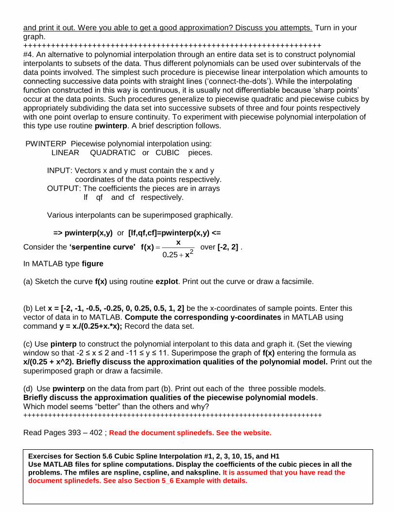
and print it out. Were you able to get a good approximation? Discuss you attempts. Turn in your graph. +++++++++++++++++++++++++++++++++++++++++++++++++++++++++++++++++ #4. An alternative to polynomial interpolation through an entire data set is to construct polynomial interpolants to subsets of the data. Thus different polynomials can be used over subintervals of the data points involved. The simplest such procedure is piecewise linear interpolation which amounts to connecting successive data points with straight lines (‘connect-the-dots’). While the interpolating function constructed in this way is continuous, it is usually not differentiable because ‘sharp points’ occur at the data points. Such procedures generalize to piecewise quadratic and piecewise cubics by appropriately subdividing the data set into successive subsets of three and four points respectively with one point overlap to ensure continuity. To experiment with piecewise polynomial interpolation of this type use routine pwinterp. A brief description follows. PWINTERP Piecewise polynomial interpolation using: LINEAR QUADRATIC or CUBIC pieces. INPUT: Vectors x and y must contain the x and y coordinates of the data points respectively. OUTPUT: The coefficients the pieces are in arrays lf qf and cf respectively. Various interpolants can be superimposed graphically.

=> pwinterp(x,y) or [lf,qf,cf]=pwinterp(x,y) <=

Consider the ‘serpentine curve' 20 25

xf(x)

. x

over [-2, 2] .

In MATLAB type figure (a) Sketch the curve f(x) using routine ezplot. Print out the curve or draw a facsimile. (b) Let x = [-2, -1, -0.5, -0.25, 0, 0.25, 0.5, 1, 2] be the x-coordinates of sample points. Enter this vector of data in to MATLAB. Compute the corresponding y-coordinates in MATLAB using command y = x./(0.25+x.*x); Record the data set. (c) Use pinterp to construct the polynomial interpolant to this data and graph it. (Set the viewing window so that -2 ≤ x ≤ 2 and -11 ≤ y ≤ 11. Superimpose the graph of f(x) entering the formula as x/(0.25 + x^2). Briefly discuss the approximation qualities of the polynomial model. Print out the superimposed graph or draw a facsimile. (d) Use pwinterp on the data from part (b). Print out each of the three possible models. Briefly discuss the approximation qualities of the piecewise polynomial models. Which model seems “better” than the others and why? ++++++++++++++++++++++++++++++++++++++++++++++++++++++++++++++++++++++++

Read Pages 393 – 402 ; Read the document splinedefs. See the website.

Exercises for Section 5.6 Cubic Spline Interpolation #1, 2, 3, 10, 15, and H1 Use MATLAB files for spline computations. Display the coefficients of the cubic pieces in all the problems. The mfiles are nspline, cspline, and nakspline. It is assumed that you have read the document splinedefs. See also Section 5_6 Example with details.

H1. Section 5.6 The 1995 Kentucky Derby was won by a horse named Thunder Gulch in a time of 2:01 1/5 (2 min 1 and 1/5 sec) for the 1.25 mile race course. Times at the quarter mile, half-mile, and mile poles were 22.4 secs, 45.8 secs, and 1 min 35.6 secs. a) Use the previous data together with the initial data, t = 0, dist = 0, to construct a natural cubic spline for Thunder Gulch's race. b) Use the spline to predict the time at the three-quarter-mile pole, and compare this to the actual time of 1 min 10.2 secs. c) Use the spline to predict the speed at which Thunder Gulch left the starting gate and the speed at which he crossed the finish line. Give answers in miles per hour. Show all your work. For #1, discuss the question also discuss the type of relationship between z an T implied by the spline. For #2, discuss the question also discuss the type of relationship between z an p implied by the spline. For #10 use the MATLAB routines to generate the requested graphs. Include a copy of the graphs as part of your solution. For #15, include a graph of the error for the natural cubic spline. +++++++++++++++++++++++++++++++++++++++++++++++++++++++++++++++++ Read pages 405-418

For #8 use MATLAB routine pwhermitecubic.m . For #10 use MATLAB routine cspline.m . IMPORTANT: For Dr. Hill’s problems use the generalization of divided differences to compute any Hermite interpolation polynomial. Show the divided difference tables for each problem. 1. The following sample of function f is given. a) Approximate f(0.5) using a polynomial interpolant. b) Approximate f(0.5) using a Hermite interpolant.

c) The function sample is from f(x) = 2xex – e

3x. Compute the absolute error in each of the results

from parts a and b. d) Graph the absolute error expressions for parts a and b over [-1,1]. Comment on the accuracy of part a vs that in part b. 2. A switching track is to be constructed between a pair of parallel trolley tracks as shown in the figure. The transition between the two tracks is to be smooth. Assume that the tracks are horizontal and the switch points have coordinates (3,2) and (0,0) on tracks #1 and #2 respectively. Construct a Hermite interpolating polynomial that goes through the points and matches the slope of the track at each of the two points. Generate a graph of your “track” over [0,3].

Section 5.7 Hermite Interpolation and Cubic Hermite Interpolation #8, 10 (in the text) There is an mfile for the data set for #8 & 10; Bradie_data_Sec5_7_Exer8.m Dr. Hill’s problems #1, 2, 3

x f(x) f’(x)

-1 -.79 -.15

0 -1.0 -1.0

1 -14.6 -49.0

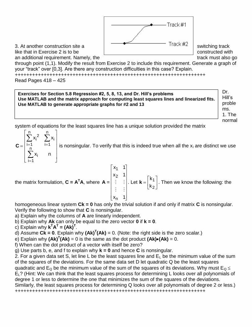
3. At another construction site a switching track like that in Exercise 2 is to be constructed with an additional requirement. Namely, the track must also go through point (1,1). Modify the result from Exercise 2 to include this requirement. Generate a graph of your “track” over [0,3]. Are there any construction difficulties in this case? Explain. ++++++++++++++++++++++++++++++++++++++++++++++++++++++++++++++++++ Read Pages 418 – 425

Dr. Hill’s problems. 1. The normal

system of equations for the least squares line has a unique solution provided the matrix

C

L

N

MMMMM

O

Q

PPPPP

x x

x n

i2

i 1

n

i

i 1

n

i

i 1

n is nonsingular. To verify that this is indeed true when all the x i are distinct we use

the matrix formulation, C = ATA, where =

x 1

x 1

x 1

1

2

n

A

L

N

MMMMMM

O

Q

PPPPPP

. Let k LNMOQP

k

k

1

2

. Then we know the following: the

homogeneous linear system Ck = 0 has only the trivial solution if and only if matrix C is nonsingular. Verify the following to show that C is nonsingular. a) Explain why the columns of A are linearly independent. b) Explain why Ak can only be equal to the zero vector 0 if k = 0. c) Explain why kTAT = (Ak)T. d) Assume Ck = 0. Explain why (Ak)T(Ak) = 0. (Note: the right side is the zero scalar.)

e) Explain why (Ak)T(Ak) = 0 is the same as the dot product (Ak)(Ak) = 0. f) When can the dot product of a vector with itself be zero? g) Use parts b, e, and f to explain why k = 0 and hence C is nonsingular. 2. For a given data set S, let line L be the least squares line and EL be the minimum value of the sum of the squares of the deviations. For the same data set D let quadratic Q be the least squares

quadratic and EQ be the minimum value of the sum of the squares of its deviations. Why must EQ EL? (Hint: We can think that the least squares process for determining L looks over all polynomials of degree 1 or less to determine the one that minimizes the sum of the squares of the deviations. Similarly, the least squares process for determining Q looks over all polynomials of degree 2 or less.) ++++++++++++++++++++++++++++++++++++++++++++++++++++++++++++++++++

Exercises for Section 5.8 Regression #2, 5, 8, 13, and Dr. Hill’s problems Use MATLAB and the matrix approach for computing least squares lines and linearized fits.

Use MATLAB to generate appropriate graphs for #2 and 13

Assignments for Bradie Chapter 6 2016 Assignments for Sections 6.1 and 6.2 Section 6.1 #1, 2, 3 (Yo need to use software here.) For #1: Rather than compute the not-a-knot cubic spline, just do the following. Assume you have computed S(θ) the not-a-knot cubic spline. Explain how to actually determine a

graph of S

S

'( )

( )

which approximates μ (the coefficient of friction) for 0 5 . Give details of the

procedure.

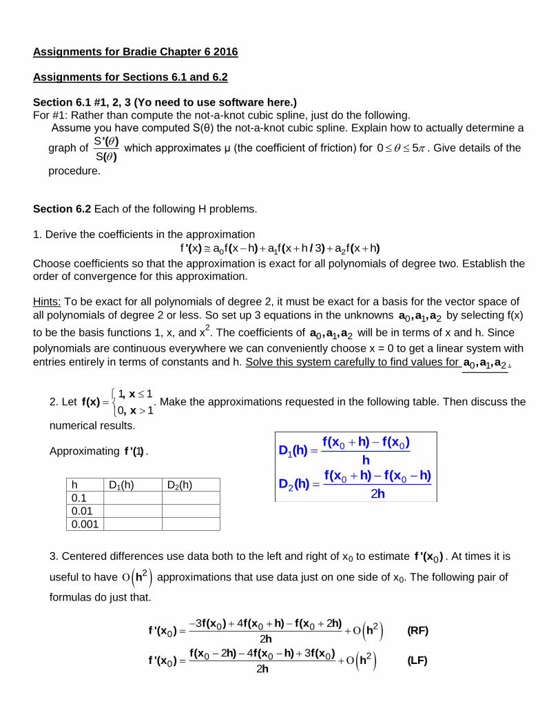
Section 6.2 Each of the following H problems. 1. Derive the coefficients in the approximation

0 1 2f x a f x h a f x h 3 a f x h'( ) ( ) ( / ) ( )

Choose coefficients so that the approximation is exact for all polynomials of degree two. Establish the order of convergence for this approximation. Hints: To be exact for all polynomials of degree 2, it must be exact for a basis for the vector space of

all polynomials of degree 2 or less. So set up 3 equations in the unknowns 0 1 2a ,a ,a by selecting f(x)

to be the basis functions 1, x, and x2. The coefficients of 0 1 2a ,a ,a will be in terms of x and h. Since

polynomials are continuous everywhere we can conveniently choose x = 0 to get a linear system with

entries entirely in terms of constants and h. Solve this system carefully to find values for 0 1 2a ,a ,a .

2. Let 1 1

0 1

, xf(x)

, x

. Make the approximations requested in the following table. Then discuss the

numerical results.

Approximating 1f '( ) .

3. Centered differences use data both to the left and right of x0 to estimate 0f '(x ) . At times it is

useful to have 2h approximations that use data just on one side of x0. The following pair of

formulas do just that.

20 0 00

20 0 00

3 4 2

2

2 4 3

2

f(x ) f(x h) f(x h)f '(x ) h (RF)

h

f(x h) f(x h) f(x )f '(x ) h (LF)

h

0 01

f(x h) f(x )D (h)

h

0 02

2

f(x h) f(x h)D (h)

h

h D1(h) D2(h)

0.1

0.01

0.001

For the data in the following table use formulas RF or LF to estimate f '(x) . For each value of x

indicate which formula you used.

x f(x)_______________Estimate of f '(x)__ (RF or LF) 2 9.20765095258201 2.2 10.8037055878372 2.4 12.6442880139644 2.6 14.8040416017375 2.8 17.3826135915336 3 20.5088969473673

4. For any reasonable formula that estimates f '(x) as a linear combination of function values of f like

1

n

k k

k

f '(x) A f(x )

Explain why

1

0

n

k

k

A

.

5. In a circuit with impressed voltage E(t) and inductance L, Kirchoff’s first Law gives the

relationship di

E t L Ridt

( ) where R is the resistance in the circuit and i is the current. Suppose

we measure the current for several values of t and obtain Where t is measured in seconds, I is in amperes, the inductance L is a constant 0.98 henries, and the resistance is 0.142 ohms. Approximate the voltage E at the values of t given in the table. Use second order (3 point) formulas. (Show your work including the formula used for each value of t.)

Read Pages 455-466

For 1c, do this problem using your calculator for computations. Show your work.

For 9 This problem needs hand calculations; do not use approximations to 3

3, do things exactly.

For 6, part (a) use f = 1, x, x2 and the definition of degree of precision to set up a system of equation to solve for the coefficients. Express the coefficients as rational numbers. Then for part (b) you can use the constructive result from part (a) to shorten the search for the degree of precision. ++++++++++++++++++++++++++++++++++++++++++++++++++++++++++++++++++ Read Pages 467-478

t 1.00 1.01 1.02 1.03 1.04

i 3.10 3.12 3.14 3.18 3.24

Exercises for Section 6.4: #1c, 9, 6 (do the problems in the order listed.) Newton-Cotes

Exercises for Section 6.5: Dr. Hill’s problem H1, (text)#20 (only for Trapezoidal rule), (text)4. Composite Simpson’s Rule, DR. Hill’s problem H2 display & carry in computations at least 8 decimal values.

H1. Dr. Hill’s problem: We want to approximate using the COMPOSITE Trapezoidal

rule, Simpson’s rule, and Midpoint rule. For the sake of comparison we want to use the same value of

the h in each program (in MATLAB trap, simp, midpt). These programs are written so that you enter a

function formula f, interval of integration a to b and the number of times the basic rule integration rule

will be used. For trap , while for simp and midpt . Use each of the programs to

approximate this integral. (Use h = 0.05.)

For #4. Here you will need to make several approximations using program simp with appropriate

choices of n (see Dr. Hill’s problem above for choosing n). You need to complete the following table

and then apply formula in Exercise #3(b) page 479 to the Simpson Estimates Sh(f).

1

0 4

1dx

1 x

b ah

n

b ah

2n