some mathematics of nonrenewable resources: from...

Some Mathematics of Nonrenewable Resources:From Arithmetic to Optimal Control Theory

Some Mathematics of NonrenewableResources: From Arithmetic to Optimal

Control Theory.

Michael OlinickDepartment of Mathematics

Middlebury [email protected]

MAA Session on Integrating the Mathematics ofPlanet Earth 2013 in the College Mathematics

Curriculum, IIJanuary 9, 2013

Our current civilization is heavily dependent on nonrenewable(exhaustible) resources. We use petroleum, coal, natural gas anduranium-dependent nuclear power to create electricity, heat andcool our homes, power our vehicles and manufacture our goods.Products we use every day require minerals such as copper, gold,silver, zinc and aluminum which we use up faster than the earthcan replenish them.How long will such nonrenewable resources last? Are there optimalways to manage a dwindling supply?We will illustrate how such questions can be approached using avariety of models that can be successfully integrated into a rangeof courses including college algebra, calculus of one and severalvariables, differential equations, discrete dynamical systems,computer simulation, and optimal control theory.

Limits To Growth, 1972Beyond the Limits, 1992

Limits To Growth, the 30 Year Update, 2004

Graham Turner, A Comparison of the Limits toGrowth With Thirty Years of Reality, 2008

The observed historical data for 1970 - 2000most closely matches the simulated results ofthe Limits to Growth ”standard run” scenario

for almost all the outputs reported; thisscenario results in global collapse before the

middle of this century.

What is a NonrenewableResource?

Nonrenewable = Exhaustible

How To Compare ReservesUnits of Measurement

I TonsI PoundsI Troy OuncesI FlasksI BarrelsI Cubic Feet

Static Index

The Static Index sHow long will the resource last if we keep using it at

the current rate of consumption?

Assumptions:

I Known Reserve K of the Resource

I Constant rate C of Consumption

s = KC

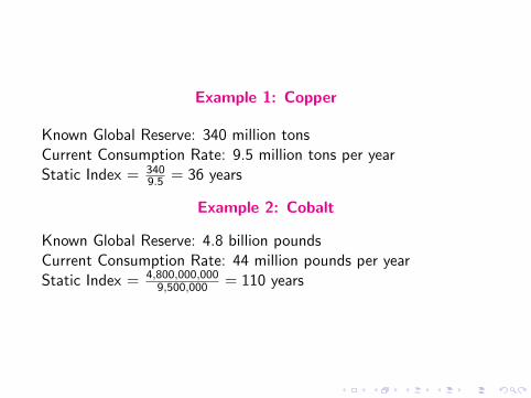
Example 1: Copper

Known Global Reserve: 340 million tonsCurrent Consumption Rate: 9.5 million tons per yearStatic Index = 340

9.5 = 36 years

Example 2: Cobalt

Known Global Reserve: 4.8 billion poundsCurrent Consumption Rate: 44 million pounds per yearStatic Index = 4,800,000,000

9,500,000 = 110 years

Example 1: Copper

Known Global Reserve: 340 million tons

Current Consumption Rate: 9.5 million tons per yearStatic Index = 340

9.5 = 36 years

Example 2: Cobalt


9,500,000 = 110 years

Example 1: Copper

Known Global Reserve: 340 million tonsCurrent Consumption Rate: 9.5 million tons per year

Static Index = 3409.5 = 36 years

Example 2: Cobalt


9,500,000 = 110 years

Example 1: Copper


9.5 = 36 years

Example 2: Cobalt


9,500,000 = 110 years

Example 1: Copper


9.5 = 36 years

Example 2: Cobalt

Known Global Reserve: 4.8 billion pounds

Current Consumption Rate: 44 million pounds per yearStatic Index = 4,800,000,000

9,500,000 = 110 years

Example 1: Copper


9.5 = 36 years

Example 2: Cobalt

Known Global Reserve: 4.8 billion poundsCurrent Consumption Rate: 44 million pounds per year

Static Index = 4,800,000,0009,500,000 = 110 years

Example 1: Copper


9.5 = 36 years

Example 2: Cobalt


9,500,000 = 110 years

Exponential Index

Exponential IndexMeasures How Long aResource Will Last if

Consumption Rate GrowsContinuously at a

Constant Percentage Rate

y(t) = Consumption Rate at time ty(0) = C Current Consumption Rate

dydt = ry

HenceConsumption Rate = Cert

y(t) = Consumption Rate at time ty(0) = C Current Consumption Rate

dydt = ryHence

Consumption Rate = Cert

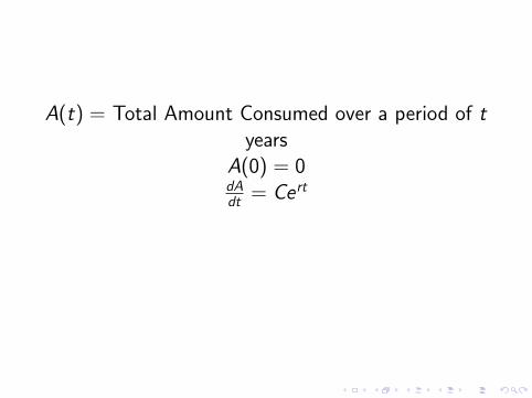
A(t) = Total Amount Consumed over a period of tyears

A(0) = 0dAdt = Cert

HenceA(t) = C

r [ert − 1]

System of DifferentialEquationsdydt = rydAdt = y

y(0) = C ,A(0) = 0

Exponential Index T is time it will take to consumethe total known global reserve K :

A(T ) = KCr [e

rT − 1] = KrKC = erT − 1

erT = 1 + rKC = 1 + rs

HenceT = ln(1+rs)

r

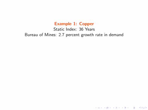
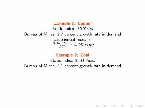
Example 1: Copper

Static Index: 36 YearsBureau of Mines: 2.7 percent growth rate in demand

Exponential Index is:ln(36∗.027+1)

.027 = 25 Years

Example 2: CoalStatic Index: 2300 Years

Bureau of Mines: 4.1 percent growth rate in demandExponential Index is:

ln(2300∗.041+1).041 = 111 Years

Example 1: CopperStatic Index: 36 Years


ln(36∗.027+1).027 = 25 Years



ln(2300∗.041+1).041 = 111 Years


Bureau of Mines: 2.7 percent growth rate in demand


.027 = 25 Years



ln(2300∗.041+1).041 = 111 Years



ln(36∗.027+1).027 = 25 Years



ln(2300∗.041+1).041 = 111 Years



ln(36∗.027+1).027 = 25 Years

Example 2: Coal

Static Index: 2300 YearsBureau of Mines: 4.1 percent growth rate in demand


.041 = 111 Years



ln(36∗.027+1).027 = 25 Years



ln(2300∗.041+1).041 = 111 Years



ln(36∗.027+1).027 = 25 Years


Bureau of Mines: 4.1 percent growth rate in demand


.041 = 111 Years



ln(36∗.027+1).027 = 25 Years



ln(2300∗.041+1).041 = 111 Years

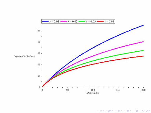
Comparing the Indices

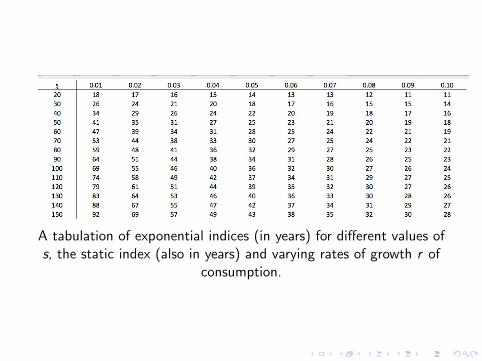
A tabulation of exponential indices (in years) for different values ofs, the static index (also in years) and varying rates of growth r of

consumption.

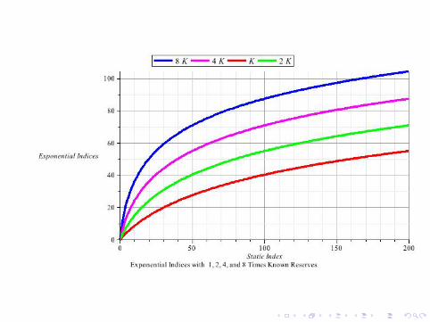
Changes inKnown Global Reserves

Actual Total Reserve = nTimes Known Reserve

T =ln(nsr+1)

r

Mineral Years Years Years YearsLomborg Benchmark Diederen Latest

0% Growth 0% Growth 2% Growth 2.57% Growth

Iron Ore 215 78 46 42Cobalt 320 91 57 46Aluminum 230 137 63 58Silver 15 23 10 18Gold 18 21 13 16Zinc 42 22 13 17Tin 47 20 15 15Copper 43 39 23 26Nickel 117 52 28 32

Table : Years of Supply Left For Certain Minerals Based On Reserves andAnnual Production Using Data from USGS Mineral CommoditySummaries, 20111

PriceMultiplier

Mineral 1989 2002 2008 2002 - 2008

Iron Ore $41.20 $23.50 $56.60 2.4

Cobalt $22,700 $15,500 $51,800 3.3

Aluminum $35.30 $18.40 $20.00 1.1

Silver $232,500 $134,000 $398,000 3.0

Gold $16,200,000 $9,060,000 $21,200,000 2.3

Zinc $2,380 $772 $1,480 1.9

Tin $15,100 $5,830 $18,900 3.2

Copper $3,800 $1,510 $5,330 3.5

Nickel $17,500 $6,130 $16,000 2.6

Table : Mineral Price Variation For Select Years; Prices in constant 1998U.S. dollars/ton. From Mark Henderson, The Depletion Wall, 2012

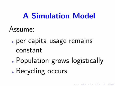
A Simulation Model

Assume:

I per capita usage remainsconstant

I Population grows logistically

I Recycling occurs

A STELLA Simulation Model

Some Details

I Resource: Copper

I Reseve: 340 million tons

I Current Population: 7 million

I per capita usage: 9.7 million/ 7 million

I Carrying Capacity: 10 million people

I Natural Growth Rate: 2 percent

I 2 percent of consumption is recycled

Population(t) = Population(t - dt) + (PopulationGrowth) * dtINIT Population = 7INFLOWS:PopulationGrowth =NaturalRate*Population*(1-Population/CarryingCapacity)Reserve(t) = Reserve(t - dt) + (Recycling - ConsumptionRate) *dtINIT Reserve = 340INFLOWS:Recycling = .03 *ConsumptionRateOUTFLOWS:ConsumptionRate = (9.5/7) *PopulationCarryingCapacity = 10NaturalRate = 0.02

Harold Hotelling1895-1973

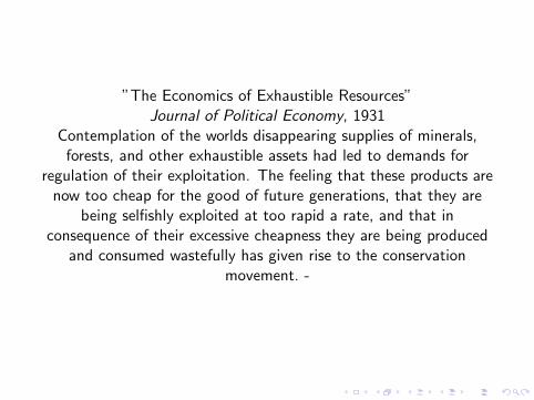
”The Economics of Exhaustible Resources”Journal of Political Economy, 1931

Contemplation of the worlds disappearing supplies of minerals,forests, and other exhaustible assets had led to demands for

regulation of their exploitation. The feeling that these products arenow too cheap for the good of future generations, that they are

being selfishly exploited at too rapid a rate, and that inconsequence of their excessive cheapness they are being produced

and consumed wastefully has given rise to the conservationmovement. -

A Simple Optimal Control Model

Xt = amount of resource in period tX0 = initial stockYt = ”harvest” levelF (Xt) = net growth rate (through recycling or exploration)πt = π(Xt ,Yt) = Net benefits in period tδ = discount ratep = 1

1+δ = discount factor

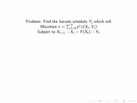
Problem: Find the harvest schedule Yt which willMaximize π =

∑Tt=0 p

tπ(Xt ,Yt)Subject to Xt+1 − Xt = F (Xt)− Yt

Problem: Find the harvest schedule Yt which willMaximize π =

∑Tt=0 p

tπ(Xt ,Yt)Subject to Xt+1 − Xt = F (Xt)− Yt

Form LagrangianL =

∑Tt=0 p

t{π(Xt ,Yt) + pλ[Xt + F (Xt)− Yt − Xt+1]}

Necessary Conditions For Maximum:∂L∂Yt

= pt{∂π(Xt ,Yt)∂Yt

− pλt+1} = 0∂L∂Xt

= pt{∂π(Xt ,Yt)∂Xt

+ pλt+1[1 + F ′(Xt)]} − ptλt = 0∂L

∂[pλt+1] = pt{Xt + F (xt)− Yt − Xt+1} = 0

More Complex Models

I Demand Functions

I Reserve-Dependent Costs

I Pollutants (Degradable and Nondegradable)

I Recycling

I Risky Development

Cambridge University Press; 2010

Other References:

I Geoffrey M. Heal, ed., Symposium on the Economics ofExhaustible Resources, The Review of Economic Studies, 41,1974.

I Partha S. Dasgupta and Geoffrey M. Heal, Economic Theoryand Exhaustible Resources, Cambridge University Press, 1980.

I Suresh Sethi and Gerald Thompson, Optimal Control Theory,Springer: 2006

I Marck C. Henderson, The Depletion Wall: Non-RenewableResources, Population Growth, and the Economics of Poverty,Waves of the Future, 2012.

I Michael Olinick, ”Modelling Depletion of NonrenewableResources,” Mathematical and Computing Modelling, 15, 91

THANK YOU

[email protected]

A model assuming that a sufficiently high price, p, a substitute willbecome available.

Example: Solar energy might substitute for fossil fuel

p(t) = price of the resource at time tq = f (p) is the demand function: the quantity demanded

at a price pp̄ = price at which substitute completely replaces the resource.c = G (q) is the cost function

Q(t) = the available stock or reserve of the resource at time t,Q(0) = Q0 > 0

r = social discount rate; r > 0T = the horizon time: the latest time at which the substitute

will become available regardless of the price of the naturalresource, T > 0

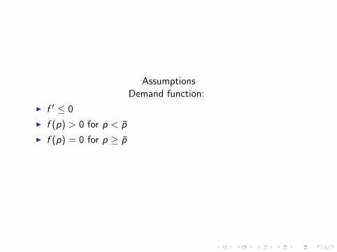
AssumptionsDemand function:

I f ′ ≤ 0

I f (p) > 0 for p < p̄

I f (p) = 0 for p ≥ p̄

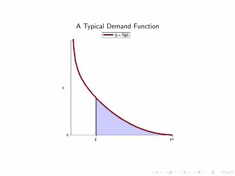
A Typical Demand Function

AssumptionsCost function G (q) (q is demand)

I G (0) = 0

I G (q) > 0 for q > 0

I G ′ > 0 and G” ≥ 0

I G ′(0) < p (producers can make positive profit at a price pbelow p̄ )

Let c = G (q) = G (f (p)) = g(p)Note: g(p) > 0 for p < p̄ and g(p) = 0 for p ≥ p̄Let π(p) = pf (p)− g(p) denote the profit function of theproducers.π is called producers’ surplusLet p be the smallest price at which π is nonnegative.We assume π(p) is concave in interval [p, p̄]Consumer Surplus:

ψ(p) =

∫ p̄

pf (y)dy

Maximize

J =

∫ T

0[ψ(p) + π(p)]e−rtdt

subject to

Q ′(t) = −f (p),Q(0) = Q0,Q(T ) ≥ 0

and

p ∈ [p, p̄]

some mathematics of nonrenewable resources: from...

Documents