Some Issues in Inflation Targeting

by

Andrew G Haldane*

*Bank of England, Threadneedle Street, London, EC2R 8AH

I would like to thank a number of my colleagues at the Bank of England, in particular Bill Allen,Clive Briault, Spencer Dale, Paul Fisher, Suzanne Hudson, Mervyn King, Charles Nolan, DarrenPain, Vicky Read, Lars Svensson, Paul Tucker, Peter Westaway and John Whitley. I would also like tothank participants at the Konstanz monetary seminar in June 1996 for which this paper waswritten, in particular my discussant Walter Wasserfallen; and an anonymous referee. Remainingerrors are of course my own, as are the views expressed within, which are not necessarily those ofthe Bank of England.

Issued by the Bank of England, Threadneedle Street, London, EC2R 8AH to which requests forindividual copies should be addressed: envelopes should be marked for the attention of thePublications Group (Telephone 0171-601 4030).

Bank of England 1997ISSN 1368-5562

2

3

Contents

Abstract 5

1 Introduction 7

2 What is new in inflation targeting? 8

3 The forward-looking nature of inflation targeting 12

4 Information requirements of inflation targeting 16

5 Forecasting inflation at the Bank of England 17

6 Inflation forecasting and probability distributions 22

7 Inflation targeting and transparency 28

8 Does inflation targeting destabilise output? 33

9 Assessing the effects of inflation targeting 35

10 Conclusions 40

References 41

4

5

Abstract

This paper discusses some of the operational issues relevant to theimplementation of an inflation-targeting regime. In particular it focuses on:whether inflation targeting is ‘new’; whether it is potentially destabilising, forexample to output; and whether it requires too much knowledge on the partof the authorities. The paper argues that none of these propositions appears ingeneral to be correct.

It goes on to discuss the use of inflation forecasts in general, and inflationprobability distributions in particular, in the context of inflation targeting inthe United Kingdom. It also discusses the important role greater transparencyplays among inflation targeters and discusses some evidence on this. Finally,a preliminary evaluation of inflation targeters’ performance to date is given.

6

7

1 Introduction

This paper is intended as a ‘cookbook’ of the hows, whys and wherefores ofinflation targeting. Of itself, that does not make the paper novel. There arealready surveys aplenty: on the genesis of inflation targets (Ammer andFreeman (1995), Haldane (1995a)); on comparisons between inflationtargets and alternative monetary regimes (McCallum (1995a), Cukierman(1995)); on the analytics of inflation targeting (Svensson (1996), Cukierman(op cit); and on some of the specification issues raised by these regimes(Bank of Canada (1994), Goodhart and Vinals (1994), McCallum (op cit),Haldane and Salmon (1995), Yates (1995), Haldane (1997)). Meanwhile,two recent books describe the practical experience of countries operatingunder an inflation target (Leiderman and Svensson (1995), Haldane (1995b));and Almeida and Goodhart (1996) provide a comprehensive recent evaluationof the performance to date of inflation-target countries.

Our aims here are more modest and parochial: to describe some of themodalities of inflation targeting as currently operated in the United Kingdomand, to a lesser extent, elsewhere. Duguay and Poloz (1994) conduct asimilar exercise for Canada. In doing so, we side-step some of the theoretical- or ‘time-consistency’ - issues raised by the use of inflation targets andconcentrate on the ‘engineering’ side of policy. Time-consistency issues areimportant but are amply dealt with elsewhere (inter alia, King (1996),Haldane (1995c), Svensson (1995b)). Looked at from an operational angle,the differences between - on the face of it - competing monetary strategiesare probably more apparent than real. That said, there are some respects inwhich inflation targeting does help force some new engineering issues intothe open - such as in the use of explicit, probabilistic forecasts in the settingof monetary policy. A number of these issues are explored here, with explicitreference to the United Kingdom.

The paper is set out as follows: sections 2-4 discuss whether inflationtargeting is ‘new’; whether it is potentially destabilising; and whether itrequires too much knowledge on the part of the authorities. Sections 5 and 6discuss the role of inflation projections in the formulation of UK monetarypolicy. Sections 7 and 8 discuss whether inflation targeting may be either‘black box’ or may destabilise output. Section 9 evaluates the performance ofinflation-target countries to date; and Section 10 briefly concludes.

8

2 What is new in inflation targeting?

Because inflation targets are a creation of the 1990s, many view them as awholly new monetary policy strategy - and, as such, one with a low accruedstock of credibility. That impression was no doubt given weight by thecircumstances in which most countries adopted inflation targets. Typically,this came either as a response to an unexpected unhinging of an earliermanaged exchange rate regime - as in Finland (Brunila and Lahdenpera(1995), and Sweden (Andersson and Berg (1995), Svensson (1995a)); or as aresult of the failure of monetary targeting owing to the vicissitudes of moneyvelocity during the 1970s and 1980s - as, for example, in Canada (Freedman(1994)) and New Zealand (Fischer (1995), McCallum (1995b)); or, in theUK case, as a result of both (Bowen (1995), King (1994)).

But it would be incorrect to overplay the novelty of inflation targeting, for twoquite separate reasons. First, history tells us that inflation targeting is notentirely new. The intellectual roots of price targets can be traced back to thelast century - to Marshall (1887) and Wicksell (1898). Later, Fisher (1911)and Keynes (1923) both put forward monetary policy schemes which targetedexplicitly an index number for prices. So, to take Keynes (1923, page 148):

‘....it would promote confidence and furnish an objective standard ofvalue, if, an official index number having been compiled...to registerthe price of a standard composite commodity, the authorities were toadopt this composite commodity as their standard ofvalue...prevent[ing] a movement of its price by more than a certainpercentage in any direction away from the normal’

Such schemes were the forerunner of Sweden’s experiment with an explicitprice-level standard during the early part of the 1930s (Jonung (1979)). Andsuch experiments were in turn the intellectual and practical forerunners ofprice targets today. Of course, one respect in which the debate ‘then’ and‘now’ is different is that then a numerical target for the price level was beingadvocated, whereas now numerical targets are being set for the rate of changeof price levels. There has been what Flemming (1976) calls a ‘change ofgear’ in price expectations in the first and second halves of this century. Thisraises some interesting issues for the future: for example about the pros andcons of base-drift in the price level, mirroring the 1980s debate on this subjectin the context of monetary targets. But these issues are not pursued furtherhere (see Duguay (1994)), Haldane and Salmon (1995) for a discussion).

Second, from an analytical perspective, the differences between inflationtargeting and, say, monetary targeting are probably more semantic thaneconomic. After all, both regimes have the same ultimate aim: a specified

9

growth path for nominal magnitudes. And given the transmission lags inmonetary policy, both rely on a forward-looking inflationary assessment whenmonetary policy is being set. So the difference between them seems to hingeon the weights each assigns to different information variables when formingthis forward-looking inflation assessment.

In theory, the differences are acute. Pure monetary targeting is a limitingcase of inflation targeting, where the weight attached to monetary variables isunity and that attached to non-monetary variables is zero. Conversely,inflation targeting means using an eclectic mix of information variables, withnon-zero weights assigned to both real and monetary magnitudes whenforming an inflationary assessment. Pure monetary targeting would, by thistaxonomy, simply be inflation targeting with indicator weight restrictions of(0, 1) imposed.

Yet, in practice, this distinction and these restrictions are largelyhypothetical. Studies of the Bundesbank’s reaction function (such as Claridaand Gertler(1995), Muscatelli and Tirelli (1996), Neumann (1995), Schachterand Stokman (1995)) confirm that real as well as monetary variables help toexplain its actions over recent years. Indeed, strikingly, actual and expectedinflation and output gaps are often found to play a prominent explanatory rolewith money having, at best, a bit part. There seems to be nothing ‘pure’about monetary targeting in practice. Indeed, some have ventured to suggestthat monetary targeting is inflation targeting in all but name (Clarida andGertler (1995), Bernanke and Mihov (1996)). This makes perfect sense sinceboth monetary and non-monetary variables have a role to play in accountingfor inflationary dynamics over the policy effectiveness interval - the 18-monthto 2-year period over which monetary policy has its maximum effect oninflation (see, eg, Cechetti (1995)).(1) A (0, 1) weighting scheme forindicators in the reaction function is simply not supported by the data.

To offer some illustrative empirical evidence on the contribution of real andmonetary variables in explaining inflation dynamics, consider some blockexogeneity tests and variance decompositions from a four-variable VAR forthe United Kingdom comprising: RPIX (the price level); import prices

(1) When discussing the indicators on which the monetary authorities should base their policydecisions, Keynes (1923, page 149) lists:

‘Actual price movements must of course provide the most important datum; but the state of employment, the volume of production, the effective demand for credit as felt by banks, the rate of interest on investments of various types, the volume of new issues, the flow of cash into circulation, the statistics of foreign trade and the level of the exchanges must all be taken into account’.

10

(IMP); a monthly activity proxy - the unemployment rate (UN); (2) and avariety of variables proxying the ‘monetary stance’ - narrow money (MO,VAR 1 in Table A), broad money (M3 , VAR 2) and nominal interest rates(INT, VAR 3). The sample period is January 1975 to December 1995 and thedata are monthly.

Table AVariance decompositions of RPIX inflation

VAR 1 C o n t r i b u t i o n s o f ( p e r c e n t )H o r i z o n

( m o n t h s )R P I X I M P U N M 0

12 84 10 2 324 61 20 4 1636 31 12 26 3148 16 6 47 31

VAR 2 C o n t r i b u t i o n s o f ( p e r c e n t )H o r i z o n

( m o n t h s )R P I X I M P U N M 3

12 76 6 2 1624 56 8 15 2136 34 6 43 1748 23 5 59 13

VAR 3 C o n t r i b u t i o n s o f ( p e r c e n t )H o r i z o n

( m o n t h s )R P I X I M P U N INT

12 84 7 15 324 58 12 22 836 35 10 49 648 23 7 62 7

Block exogeneity tests (not reported) indicated a strong role for both the realand monetary variables in accounting for inflationary dynamics, each beingadmissible at at least the 5% significance level, and often at much higherlevels of significance. We can get some feel for the temporal dynamiceffects of these variables upon RPIX by looking at variance decompositions.These are shown in Table A at four horizons - 12, 24, 36 and 48 months.(3)

The general pattern is of inflationary inertia - lagged inflation - being thedominant inflationary influence over the first year or so. Import prices alsohave their strongest effect over the shorter run - somewhere between one andtwo years out. Activity variables kick in strongly over the medium term -between, say, two and four years out; while the monetary variables typicallybring up the rear, though their effect can also be strong - dominant, in fact - (2) Using industrial production - a noisier monthly activity series - gave less clear but similarresults.(3) The ordering is as in Table A: inflation; import prices; activity; and the monetary variables.

11

over longer horizons. These conclusions are broadly consistent with thefindings of Lougani and Swagel (1995) in a VAR-based study of inflationarydynamics in the OECD. Although classical monetary forces assertthemselves over the long run, both real and monetary factors remain centralto explaining inflationary dynamics over medium-term horizons.(4) Takentogether, this evidence suggests that non-monetary variables have a well-defined role to play in accounting for inflationary dynamics over the policyeffectiveness interval. That would argue persuasively for their inclusion -implicitly or explicitly - in the reaction function of any central bank seekingprice stability. Again, the restrictions implied by a (0, 1) indicator-weightingscheme are not justified by the data.

Theoretical support for choosing a mix of information variables is strongerstill. It is well-known that the optimal feedback rule combines a diversifiedset of information variables (Friedman (1975)). Inflation targeting, by usingsuch a diversified mix, can be seen as an attempt to mimic this optimalfeedback rule.(5) This approach could in principle come across as confusingand random. It may appear, for example, that the monetary authorities areassigning indicators different weight at different times; that they are pickingand choosing as they see fit. But according to control theory, such behaviouris simply the optimal response to the wide range of shocks affecting themedium-term inflation profile. The rule itself - if not the implications forpolicy - are invariant to the particular realisation of shocks. Far from beingrandom, such a ‘case-by-case’ approach is entirely in keeping with whatcontrol theory would tell us was optimal.

By contrast, feeding back from a single indicator - be it money, the exchangerate or whatever - is to restrict arbitrarily and unnecessarily the argumentsentering the feedback rule. Because that means discarding information usefulfor predicting future inflation, it can never be optimal in a control theorysense. (6) Of course, given the flexible way in which monetary targeting hasoperated in practice, this drawback of intermediate targeting need not bedecisive. It is these considerations that ultimately lead King (1996) topropose a ‘fundamental equivalence theorem’ between all intermediatetargeting strategies - both in theory and in practice. So while inflationtargeting may sound new, in fact much of what it comprises should befamiliar enough from history or from existing monetary regimes.

(4) These responses are also consistent with the temporal patterns from the Bank’s forecastingmodel.(5) Svensson (1996) shows that forward-looking inflation targeting secures the minimum varianceof inflation.(6) See, again, Svensson (1996).

12

3 The forward-looking nature of inflation targeting

The most common early criticism of inflation targeting was that it wasbackward-looking; that, by feeding back from actual inflation, monetarypolicy was ‘driving the economy by looking out of the rear-view mirror’.Described in this way, such a strategy does indeed sound like a recipe fordisaster, failing as it does to take account of the transmission lag between theenactment of monetary policy and its ultimate impact on prices. In Keynes’(1923) words: ‘...if we wait until a price movement is actually afoot beforeapplying remedial measures, we may be too late’. Certainly, if actualinflation is the long and variable tail on the end of the monetary policy dog,then a policy of chasing one’s tail is, at best, thankless and, at worst,destabilising. And the monetary policy equivalent of chasing one’s tail is togenerate - possibly destabilising - inflationary cycles. An analytical exampleof such behaviour is given below.

In practice, this view of inflation targeting is misconceived. The monetaryauthorities in inflation-target countries feed back from expected, rather thanactual, inflation. For example, in the United Kingdom the Bank of Englandpublishes in its Inflation Report an inflation projection up to two years ahead -the period at which monetary policy has its maximum marginal impact. Thisprojection, and in particular any deviation between this projection and theinflation target, then forms the basis of the Bank’s monetary policy decisions.(7) A similar procedure is used at the Bank of Canada,(8) the Reserve Bank ofNew Zealand, and elsewhere. In effect, what occurs among inflation-targeting central banks is inflation forecast targeting, with the forecast takingthe role of feedback variable.(9) In this way, the lags embedded in themonetary transmission process are explicitly recognised in the setting oftoday’s monetary policy.

This type of policy-setting behaviour can be captured in the forward-lookingfeedback monetary policy rule:

it = γ (Et π t+j - π*) (1)

(7) And in the period prior to the Bank’s operational independence formed the basis of the Bank’sadvice to the Chancellor.(8) Where they solve the dual of this problem: for the path of monetary conditions (weightedinterest and exchange rate movements) consistent with meeting inflation objectives (Longworthand Freedman (1994)).(9) Again, see Svensson (1996).

13

where it denotes the policy instrument, π t is inflation, Et is the expectationsoperator conditional on information at time t and earlier, π* is the inflationtarget, γ is a (positive) feedback parameter and j is the targeting horizon,determined by, among other things, the length of the monetary transmissionlag. As we discuss in Sections 4 and 5, Et π t+j is best thought of as the entireprobability distribution of future inflation outcomes, rather than as a singlepoint expectation.(10)

Consider a simple two-equation model of the economy:

π t = Et π t+1 + ψ yt -1 + ut (2)y t = - β (it - Et π t+1) (3)

where y t denotes real output, it are nominal interest rates, ut is a white-noiseinflation shock and ψ and β are positive coefficients. (2) is a standardexpectational Phillips curve. (3) is a conventional aggregate demand relation.For simplicity and without loss of generality we: (a) specify (2) and (3) interms of deviations from equilibrium - that is, we partial out the natural rateof output from the right-hand side of (2) and the left-hand side of (3), andspecify no ‘core’ rate of inflation in (2);(11) (b) consider only one shock -coming from the supply side, ut - but equally could have added aggregatedemand shocks to (3); and (c) normalise ψ to unity and omit any inflationaryinertia in (2). So this is a standard aggregate demand/aggregate supplymodel. Note that there are explicit lags in monetary transmission.Yesterday’s output growth affects inflation today.(12) It is these transmissionlags which justify an explicit role for forward-looking monetary policy.

To close the model we need a monetary policy rule. Consider first a rulewhich involves no feedback, but which holds the nominal interest rateconstant at i*. The solution for inflation is then:

π t = Et π t+1 - βi* + β Et-1 π t + ut (4)

the (forward) root of which is unstable under rational expectations. Theintuition here is classic Wicksell. Imagine that real interest rates are initiallyat their ‘natural’ rate. A positive inflation shock, ut, occurs which raises

(10) In which case Et defines subjective rather than mathematical expectations, in the sensedescribed below.

(11) Equation (1) is also written in the form of a deviation from equilibrium nominal interestrates.

(12) Equally, we could have embedded lags in the aggregate demand curve, (3) . See Svensson(1996) for such a model.

14

inflation and lowers the real rate of interest. The below-equilibrium realinterest rate then stokes up further inflationary pressures, lowering the realrate of interest further. This process continues in a cumulative fashion. In theabsence of a nominal interest rate adjustment, an explosive inflationary ordeflationary spiral is set off - entirely in keeping with Wicksell’s cumulativeprocess.

Consider next the solution for inflation with the forward-looking feedback rule(1) in place:

π t = Et π t+1 + βγπ* - β(γ - 1) Et-1 π t + ut (5)

Under rational expectations, the forward root is now stable for γ > 1. (13) Againthe intuition is straightforward. To get inflation back to equilibrium followinga positive shock, real interest rates need to be raised above their natural ratetemporarily. That, in turn, means adjusting nominal interest rates by morethan any inflation shock - hence γ > 1.

As a third case, consider now a ‘chasing your tail’ policy feeding back fromcurrent inflation:

it = γ (π t - π*) (6)

π t = Et π t+1 - βγ π t-1 + β Et-1 π t + βγπ* + ut (7)

where (7) is the reduced form for inflation, given (6). We can solve thissecond-order expectational difference equation formally using the method ofundetermined coefficients.(14) Guessing a solution in the (minimum number of)predetermined state variables:

π t = φ0 + φ1 π t-1 + φ2 ut (8)

Running the expectations operator through (8) gives us expressions for Et π t+1

and Et-1 π t, thus:

Et π t+1 = φ0 + φ1 π t (9)

(13) This can be shown formally using the method of undetermined coefficients, as illustratedbelow.

(14) Though the intuition underlying the result is straightforward given that (7) is a higher-

order difference equation than (5) .

15

Using (7)-(9) and equating coefficients gives us the following undeterminedcoefficient constraints:

φ0 = βγπ* + φ0φ1 + φ0 (1 + β) (10)

φ1 = φ12 + βφ0 - βγ (11)

φ2 = 1 + φ1φ2 (12)

From (8), the key stability constraint is (11) which has the solution:

φ1 = 1 ± √ (1 + 4 β γ (1 + β ) -2 ) (13) 2 (1 + β) -1

As we would expect, this second-order system has two roots. FollowingMcCallum (1983), we choose the root which rules out ‘bubble’ solutions;that is, the value of (13) that gives φ1 = 0 whenever β = 0. This is thenegative root. Evaluating (13) then tells us that φ1 will be unambiguouslynegative. But φ1 < 0 in (8) means that inflation will be oscillatory. A‘chasing your tail’ feedback rule will itself generate inflationary cycles - andthe larger the feedback, the larger these cycles. Indeed, at high values of γ ,these oscillations could become explosive. Clark, Laxton and Rose (1995)conduct some empirical simulations of rules similar to (1) and (6). They findthat the myopic rule, (6), results in greater cyclical output swings than theforward-looking rule, (1), which mirrors our analytical finding here.(15)

These results tell us two things. First, about the dangers of following a purelybackward-looking inflation rule. Following a backward-looking inflation rulerisks introducing a further dynamic into the inflation process, rather thansubtracting one from it. Monetary policy needs to be forward-looking if it isnot to be destabilising, with the degree of forward-lookingness dictated by thetransmission lag. Second, even a forward-looking inflation rule may require aprompt and proactive policy response to secure inflation stability.(16)

(15) Few other empirical studies have tackled this forward-looking versus backward-lookingpolicy rule issue, most tending to deal with myopic policy rules (inter alia, the contributions inBryant, Hooper and Mann (1993), and Haldane and Salmon (1995)). As a result, such studiesprobably unfairly disadvantage inflation targeting in comparison with alternative policy rulesin counterfactual simulations.(16) Though, following Brainard (1967), adding uncertainty to the parameters of the model mightlower the optimal speed of policy adjustment.

16

4 Information requirements of inflation targeting

Because inflation targeting involves feeding back from the expectation offuture inflation, it clearly requires the central bank to form a view of thewhole monetary transmission process. In equations (2) and (3), monetarytransmission is fully summarised in the aggregate demand (β) and aggregatesupply (ψ) parameters, which therefore appear in the inflation reduced form.But in practice a macromodel will embody multiple parameters of interest. Ifthese parameters were poorly understood and uncertain - which in practice, ofcourse, they are - that could pose problems for a policy rule such as (1).

But, in practice, any feedback rule requires the authorities to form a viewabout the monetary transmission process. Otherwise there is no way for theauthorities to gauge how their actions will affect inflationary dynamics - thefinal objective - since these depend on all the parameters in the reduced formof the model. An understanding of the transmission process needs to underpinany monetary policy decision, irrespective of whether these actions are basedupon tomorrow’s, today’s or yesterday’s data. For example, consider amonetary feedback rule:

it = θ (mt - m*) (14)

where we assume current-period money (growth) outturns, mt, are observable,m* is the monetary target and θ is a positive coefficient. Consider also themoney demand function:

mt = π t + y t - λit + υt (15)

which is unit income elastic, homogenous in prices (here inflation) and issubject to money demand shocks, υt. Using (2), (3), (14) and (15) gives us asolution for inflation:

π t = Et π t+1 + δ Et-1 π t - δξ [π t-1 - m* + υt-1 ] + ut (16)

where δ ≡ β/(1+βξ) and ξ ≡ (θ-1 + λ). Comparing (16) with (5), it is clear thatthe inflation-stabilisation problem - the choice of feedback parameter θ - ismade no easier by adherence to the money feedback rule, (14). Inflationdynamics still depend on the full reduced form of the model, inclusive of thepolicy rule. Indeed, the inflation-control problem for the central bank couldbe made more acute if velocity shocks, υt, are significant, since these are nolonger fully accommodated under money targeting. Monetary targeting alsoclearly places a strong reliance on knowledge of the interest elasticity ofmoney demand. This is one of the less well-specified behavioural parameters

17

in macroeconomics; and is apt to be affected by financial liberalisation. Sothe informational demands of a monetary feedback rule are never less thanunder inflation targeting. The policy-maker certainly cannot abdicateresponsibility for understanding the monetary transmission mechanism byfollowing such a rule.

As for the stability of a money feedback rule, we can solve (16) using thesame method as earlier. This gives us a restriction on φ1:

φ1 = 1 ± √ (1 + 4 δ ξ (1 - δ ) -2 ) (17) 2 (1 - δ) -1

which is again likely to generate oscillatory cycles, for the same reasons asthe current-inflation feedback rule.

Of course, if money outturns today were a perfect predictor of inflationtomorrow, then the situation would be different. But this is hardly a likelyoutcome (Table A). And even if it were, then the rule (1) would simplycollapse into (14), and monetary and inflation targeting would have an exactcorrespondence. (1) nests (14) as a special case. An inflation-forecastingfeedback rule encompasses a money feedback rule. Svensson (1996)provides a formalisation of this point, illustrating that in general money-growth targeting will imply greater inflation variability than inflationtargeting.

5 Forecasting inflation at the Bank of England

Inflation targeting requires the authorities to form a conditional inflationforecast before policy choices can be decided. That is immediatelyproblematic given the difficulties involved in accurately forecasting the futurepath of almost any variable of macroeconomic interest. Friedman (1959)articulated very neatly this policy-setting dilemma in a world in whichmonetary transmission lags were long, variable and immutable:

‘[My] proposal to increase the money stock at a fixed rate month inand month out is certainly simple. Surely, you will say, it would bebetter to ‘lean against the wind’, rather than stand straight uprightwhichever way the wind is blowing. We seldom in fact know whichway the economic wind is blowing until several months after the event,yet to be effective, we need to know which way the wind is going to beblowing when the measures we take now will be effective, itself avariable date that may be half a year or a year or two years from now.

18

Leaning today against next year’s wind is hardly an easy task in thepresent state of meteorology’ (Friedman, 1959, page 93).

This meteorological analogy is particularly apposite - for inflation forecastingand weather forecasting have much in common. Both amount to decision-making under uncertainty. Both are subject to periodic shocks - for everytorrential downpour there is an equivalent terms-of-trade or indirect tax shock.But most importantly, both are essential to effective planning. News of animpending tornado would prompt actions today to batten down the hatches.Likewise, news of an impending inflationary hurricane ought to promptmonetary policy actions today to batten down demand and inflationaryexpectations. In both cases, decision-making is improved by releasingforecast information - however imperfect - and acting on it pre-emptively.

Neither science is perfect. Just as a weather forecaster cannot be certain thatthe temperature tomorrow will be exactly 18°, an economic forecaster cannotbe certain that inflation next year will be exactly 3%. Those uncertaintiescall for a probabilistic assessment of the risks and margins of error aroundforecasts. This is the direction that inflation forecasting - and monetarypolicy-making more generally - has recently taken at the Bank of England.The intermediate variable of monetary policy can be thought of as the entireprobability distribution of future inflation outcomes. As discussed in the nextsection, this allows explicitly probabilistic statements to be made about thefuture path of inflation, in an exactly analogous way to the presentation of theweather forecast.

The Bank produces two inflation projections, both of which until recentlyappeared in its quarterly Inflation Report: a short-run projection, covering thenext three months; and a medium-term projection covering the period up totwo years ahead.(17) The short-term projection provides a benchmark againstwhich the Bank can assess the inflationary ‘news’ over the quarter. The short-run projection is constructed using Kalman filter techniques. It is influencedby a combination of inflationary inertia, seasonality and a set of ‘off-model’information, such as known forthcoming changes to excise duties or othertaxes and prices.

The medium-term projection is based on a small, structural macro model,which is similar in many respects to a flex-price IS-LM model. The modelcontains around 18 behavioural equations and is described in greater detail inDhar, Fisher, Holland and Pain (1995). Stripped down to its bare bones, the

(17) The February 1996 Report for the first time did not publish a short-term inflation projection,with attention focusing on the Bank’s medium-term projection.

19

reduced form for inflation (aggregate supply) and aggregate demand impliedby the model is:

π t = α(L) π t

+ β(L) ∆wt + χ (y - y*) t

-1 + δ(L) xt + φ Et (π t

+j) + ε t

1(18)

y t = y* + γ (it - π t) + η(L) ft + ϕ(L) y t o + µ(L) qt + ξ(L) we t + ε t

2 (19)

where wt are wages; y* is potential output; xt is a vector of exogenousvariables (eg, import price inflation); it are nominal interest rates; ft definesfiscal policy; y t

o is overseas output; we t is wealth; and qt is the realexchange rate. So the reduced form of inflation, (18), is essentially anexpectational Phillips curve.(18) This is vertical in the long run. But it isresponsive to cost pressures over the short run (through α, β and δ), whetherexternal (through import price inflation) or internal (through wages); and todemand pressures - the ‘output gap’ - wealth and hence monetary policy (viaχ, γ and ξ) over the medium term. This temporal sequencing within theinflation process is similar to that found from the unrestricted VARs earlieron.

The price expectations term in (18) encompasses a range of ‘off-model’information. These are variables which are not easily incorporated into astructural model such as (18)-(19), but which nonetheless offer usefulinformation on future prices - whether the central expectation of futureinflation or the probability distribution around it. Surveys of various sorts - ofinflation expectations, of industrialists’ expectations and intentions and ofviews expressed to the Bank’s Agents around the United Kingdom - are onesuch piece of information. The money and credit aggregates are another. Thelinks from money and credit to activity and inflation in the forecasting modelare often indirect, for example working through wealth. Treating them as an‘off-model’ - expectational - influence on the forecast helps to give them amore direct role.

Inflation expectations inferred from the yield curve are another ‘off-model’indicator. Monetary policy does not feed back in any mechanical way frommarket inflation expectations. Such an approach may leave the inflation rateundetermined (see Woodford (1994) for a formalisation of this point). Itwould also fall foul of what Samuelson recently called the ‘monkey in themirror’ syndrome: central banks (the monkeys) believing that signals fromthe yield curve (their own reflection) are providing them with newinformation. But inflation expectations can provide a useful metric of, amongother things, monetary policy credibility - of the extent to which agents (18) Longworth and Freedman (1995) report a similar inflation reduced-form from the Bank ofCanada’s forecasting model.

20

believe that stated inflation objectives will be realised, or of the risks whichagents attach to these objectives not being met.

For example, in May 1995 the Governor of the Bank of England and theChancellor of the Exchequer disagreed on monetary policy. The latter’s view- not to raise interest rates - prevailed. (19) It was interesting to observe theresponse of measured longer-run inflation expectations immediately followingthis event.(20) They rose steadily for several months afterwards - perhaps anindication of policy credibility having been dented (see Chart 1). That sort ofinformation is worth knowing even if, ultimately, it is not the sort of ‘news’you would want actively to respond to with monetary policy.

Governor / Chancellor meeting of 5 May 1995

93 94 951992 96

Governor / Chancellor meeting of 5 May 1995

Per cent

Per cent

93 94 951992 96

3.5

4.0

4.5

5.0

5.5

6.0

6.5

7.0

6

7

8

9

10

11

12

13

14

15

UK Implied bond market volatility (five-day moving average)

Ten-year implied UK forward inflation rates (five-day moving average)

Chart 1

(19) This was in the period prior to the Bank’s operational independence.(20) Inflation expectations are proxied here by the ten-year forward inflation rate, derived from thedifference between the nominal and index-linked yields curves in the United Kingdom. See Deaconand Derry (1994).

21

The general point here is that the Bank’s published inflation projection is nota mechanical extrapolation from a single macro model. Rather, it draws upona much wider and richer set of information variables - quantitative andqualitative, real and monetary. Indeed, increasingly the Bank’s publishedprojection is also drawing on a wider set of models, as well as informationvariables. For example, four of the largest inflation shocks which the UnitedKingdom has encountered since it began targeting inflation are: the rise ininput prices in the second half of 1994 and the beginning of 1995; sterling’sdepreciation in the first half of 1995; the rise in broad monetary growth from1995 onwards; and the appreciation of sterling during 1996/97. In each case,detailed sectoral models complemented the information from the Bank’smedium-term forecasting model. So in the case of the input price rise, theBank drew upon VAR models to assess the historical supply chain linkagesbetween input prices, output prices and, ultimately, retail prices. Likewise,for the exchange rate shocks in 1995 and in 1996/97, the Bank drew upon asmall analytical - calibrated Dornbusch - model to pin down the potentialcauses of the exchange rate movement and to back out their inflationaryimplications; it also used structural VAR models (Astley and Garrett (1996)).For the recent money supply shock, the Bank has drawn upon separatelyestimated sectoral money demand functions to gauge the source and size ofpotential inflationary risks (see Thomas (1996)).

This eclectic approach to the use of models mirrors the approach when usingindicators (Whitley (1997)). Using a ‘portfolio’ of models offers insuranceagainst model uncertainties. Diversification applies as much to policy-makers when choosing among uncertain indicators and macro models as itdoes to investors when choosing among uncertain securities and asset-pricingmodels.

Finally, to turn (18)-(19) into an inflation projection we need to make someassumptions about the paths of the exogenous variables. These are threefold:

(a) fiscal policy: the projection assumes the same nominal control totalfor spending as assumed in the Government’s annual FinancialStatement and Budget Report. The implied real spending profiles arenot necessarily the same, as the Bank uses its own forecast of the GDPdeflator;

(b) overseas output and interest rates: outcomes for the major sixeconomies are fixed using VAR models, external forecast information(eg, OECD, IMF) etc; and

(c) monetary policy: the forecast assumes unchanged nominal interestrates over the forecast horizon.

22

The last assumption is by far the most contentious. The thinking behind it isas much expositional as analytical. Analytically, for example, there is thefamiliar Sargent and Wallace (1975) problem that constant nominal interestrates may well leave the long-run price level indeterminate - a point alsoillustrated in the model of equations (1)-(4).(21) The assumption also of coursemeans that there is a potential bias in the published projections: becauseforward-looking agents may make pricing decisions today using quite differentexpected interest rate assumptions to the ones used in the Bank’s forecast;because existing market interest rates, on which agents are basing borrowingand lending decisions, are also different to these assumptions; and because,in practice, interest rates are likely to change over the two-year forecasthorizon, thereby explicitly invalidating the forecast’s assumptions.

Against this, the constant interest rate assumption is useful in helping theBank decide on the appropriate direction for future interest rate moves; itprovides a clear-cut benchmark against which to evaluate the current policystance. (22) It is also easier presentationally, and more transparent, to publish aforecast under this assumption than to run an explicit reaction function -which is subjective and unlikely to be widely agreed upon; or to draw an‘ideal’ (inflation-target consistent) interest rate profile - which is unlikely tobe unique or riskless. In fact, when the Bank conducts policy simulations itwill typically use a reaction function to set the monetary policy profile.

Armed with these assumptions for the exogenous variables, and the off-modelinformation discussed above, a projection for inflation can then be derivedfrom (18)-(19).

6 Inflation forecasting and probability distributions

So how have the Bank of England’s forecasts performed? Charts 2, 3 and 4 -taken from the Bank’s February 1996 Inflation Report - compare the Bank’scentral inflation projection with actual RPIX inflation outturns during 1993,1994 and 1995. During 1993 and most of 1994, the Bank’s central forecastswere clearly too pessimistic about the path of future inflation. The forecastsmade in November 1994 and February 1995 were, by contrast, too optimistic.Forecasts made from May to November 1995 were broadly on track.Quantifying these forecasting errors to date suggests a mean (absolute) error

(21) This means there is a slight disjunction between the policy rule in (1 ) and the precise way inwhich such a rule is made operational in practice. But both represent attempts to mimic the fullyoptimal rule by reacting to all current-dated variables in the model.(22) In running their pre-FOMC forecasts, the Federal Reserve Board likewise usually assume a flatprofile for short-term interest rates, for much the same reasons given here (see Reifshneider,Stockton and Wilcox (1996)).

23

in the region of 1% one year ahead. This is not a small number. It suggeststhat there are significant uncertainties in the forecasting process. But it alsoalmost certainly overstates the problems that these uncertainties create, forseveral reasons.

First, a mean error of 1% one year ahead is far from unusual. Granger (1995)reports mean absolute errors of around 1.4% for one-year-ahead inflationforecasts by the NIESR in the United Kingdom over the eleven-year period1981-92, and of 1.6% in the United States, based on a survey of individualforecasters over the previous 22 years. By comparison, the Bank’sperformance is not bad. Indeed, there is perhaps evidence of a fall inuncertainty at lower rates of inflation - hence the smaller forecasting errorsduring 1995. The Bank of Canada have, for example, recently found someevidence for this (see Freedman and Longworth (1995)).

Second, as Chart 5 shows, while the Bank has exhibited a consistenttendency to overpredict inflation, at least in the early years, this tendencywas also shared by all other forecasters. This is often the case with macromodel-based forecasts which, because they are extrapolations of the past,tend to overpredict a variable when it is falling, and underpredict during anupturn. Indeed, on the evidence of Chart 5, the Bank’s forecasts have onoccasions clearly ‘outperformed the market’, lying consistently below themedian market forecast and sometimes lying on the right side of theinterquartile range. Moreover, in conducting these forecast comparisons thedice is typically loaded against the Bank’s projections because of theconstant interest rate assumption.(23) Outside forecasters, by contrast, are freeto put in a more plausible interest rate profile. If their interest rate projectionsfor the next two years outperform a constant interest rate assumption - ifinterest rates are anything other than a random walk - so too, on average, willtheir forecasts (ceteris paribus).

Last, and most important, the Bank’s approach has been increasingly to moveaway from thinking about the inflation projection as a single expectation.The one certain thing that can be said about forecasts is that they will bewrong. Often this is the result of shocks to variables or relations which areimpossible to predict ex ante. Given these uncertainties, the feedbackvariable for monetary policy is really better thought of as the entireprobability distribution of future inflation outcomes, including possible risksand asymmetries within this distribution.

(23) And because some outside forecasters tend to revise their forecasts almost continuously.

24

Chart 2inflation projections made in 1993and subsequent outturns

Chart 4RPIX inflation projections made in1995 and subsequent outturns

Chart 3RPIX inflation projections made in1994 and subsequent outturns

Chart 5Distribution of RPIX inflatioforecasts for 1994 Q4 (a)

Saying all of this is, of course, one thing; making it work in practice quiteanother. In the early days of the Inflation Report , risks and potentialasymmetries in the forecast distribution were captured qualitatively in thetext. Recently, however, the Bank has gone further towards making explicitits quantitative view of the subjective probability distribution for futureinflation outcomes. Since the February 1996 Inflation Report , the Bank haspublished a probability distribution for inflation up to two years ahead. Anexample is shown in Chart 6. To understand this picture, imagine aprobability density function from which 10% slices have progressively beencut away from the top downwards. Imagine then the density functionreassembled and looked at from above. The deepest-shaded central band isdesigned to encompass inflation outturns with a 10% probability. It is the top

25

slice. The progressively lighter-shaded areas, on both sides of thedistribution, then represent 10% probability contours fanning out around thecentral projection - the lower slices. The whole of the shaded area aims tocapture 90% of the subjective probability distribution of future inflationoutturns.

Chart 6RPIX inflation projection

Herein lies the correspondence with weather forecasting. The chart allowsprobabilistic statements to be made about inflation outcomes: ‘there is an x%probability of inflation lying within a range of y% to z%’ or ‘there is an x%chance of the inflation target being breached’. The latter statement is adirect analogue of the meteorological statement: ‘there is a y% chance ofrain tomorrow’. Such probabilistic statements have motivated the Bank’spolicy advice in the recent past. (24) For example, the published minutes of theSeptember and October 1996 monthly meetings between the Chancellor andthe Governor both recorded the Bank offering advice with a view to securinga ‘better-than-evens’ chance of hitting the inflation target two years hence.That is the sort of statement which is possible only with some estimate of theprobability distribution of future inflation in mind.

(24) In the period prior to operational independence.

26

The mechanics of the probability distribution can be briefly sketched.(25) It isbuilt up from the probability distributions of each of the variables - exogenousand endogenous - which feed into the inflation reduced form, (18). The shapeof these distributions is characterised by setting values for their (error)variance and skewness - the second and third moments. So for each variablethe ‘neutral’ assumptions are: that the uncertainty surrounding a variable isgiven by the historical error variance on the model equation; and that thebalance of risks around a variable is symmetric. If these neutral assumptionsheld for each model variable, the result would be a symmetric probabilitydistribution for future inflation, with error bands given by the historicalforecast errors.

Often, however, there may be evidence of a deviation from these neutralassumptions for one or more of the variables affecting the inflation projection.For example, a model equation may be running off track, suggesting apossible regime shift in behaviour; or there may be indirect ‘off-model’information of inflationary risks in the pipeline, for example from surveys,from financial market expectations or from money outcomes; or there may beone-sided risks to an exogenous variable assumption. Concentrating just onthe central inflation outcome would mean discarding this information.

These risks to the model variables are identified up-front, and then discussedand quantified in a series of meetings between the Bank’s Monetary PolicyCommittee (MPC) and various economists at the Bank. So all levels of theBank provide input into the forecasting process. In most cases, what isagreed at these meetings is a ranking of the risks to each of the modelvariables, in terms of their severity and the extent of their asymmetry. So, forexample, if the risks to a variable were felt to be highly asymmetric it mightreceive a 90/10 or 10/90 weighting, depending upon in which direction therisks were felt to lie. Likewise, the historical error variance can be re-weighted up or down, depending on whether the uncertainty surrounding avariable, or its structural relationship, was felt to be more or less acute thanin the past. The end-product is an agreed-upon skewness and varianceadjustment for each variable entering the inflation reduced form. This allowsthe Bank to characterise the shape of the probability distribution of each(exogenous and endogenous) variable. Using the weights of each of thesevariables in the model, these risks can then be translated into a probabilitydistribution for inflation itself. The distribution underlying Chart 6 is amodified normal - modified to take account of the variance and skewness of

(25) Britton and Whitley (1996) provide a detailed and comprehensive analytical discussion of thederivation of the Bank’s probability distributions.

27

its underlying determinants. But other distributional assumptions wouldprobably give similar results.(26)

The probability distribution adds value in three respects. First, it helps toemphasise the inherently probabilistic nature of forecasting and hencepolicy-making; and, in so doing, it helps de-emphasise single-pointexpectations of inflation as a measure of monetary stance. Second, it allowspriors and non-model information to have a bearing upon the policy-making process. The emphasis here is upon ‘telling stories’ through theprobability distribution - corroborated through various pieces of evidence, onand off-model - rather than on a mechanical extrapolation of moments. Andthird, it accommodates, and attempts to quantify, possible asymmetries in thebalance of inflation risks, the type of which before February 1996 werereferred to only qualitatively in the text of the Inflation Report .

Chart 6 helps to illustrate these last two points. Although the asymmetrieswere not large in February 1996, the inflation distribution is skeweddownwards slightly over the first year; and is skewed slightly upwards overthe second year. These asymmetries in turn correspond to two ‘stories’ whichcame to prominence last year: the downside risk to output posed by thepossibility of a rundown in stocks; and the upside risk to nominal demand in1997 posed by strong broad money growth. These asymmetries in thedistribution of risks are difficult to capture from conventional model-basedprojections, whose risks are symmetric. A published probability distribution -albeit a partially subjective probability distribution - helps to makesystematic and publicise the Bank’s view of these inflation risks andasymmetries at different time horizons.

(26) The published distribution is more sophisticated than is presented here. For example, theendogenous and exogenous variables are partitioned into aggregate demand and aggregatesupply blocks, to help in identifying and understanding their downstream effects on inflation.Also, the distribution accommodates covariances among the risks, since many of the risksidentified will not in practice be independent.

28

7 Inflation targeting and transparency

While straightforward in principle, the feedback rule under an inflation targetis in practice likely to be quite complex. The feedback variable is the fullprobability distribution of inflation outcomes, into which will feed a myriad ofinformation variables. This complexity confers both costs and benefits. Thebenefits derive from the use of a wide range of information variables, as underthe optimal feedback rule; it is ‘engineering-efficient’, in a Friedman (1975)sense. The costs are the loss of simplicity and thus transparency about whatmonetary policy is doing and why. This cost could be important if agentsbelieve that complexity is being used as a smokescreen for underhandedness -as a front for periodic inflation surprises. An inflation bias might then arise(see Cukierman and Meltzer (1986), Briault, Haldane and King (1996) andNolan and Schaling (1996)).

Recognising this, many inflation-targeting countries have made consciousefforts to improve the transparency of monetary policy; to spell out theirreaction functions in clearer and simpler terms than in the past. There havebeen several ways of achieving this. Perhaps the most important has been theannouncement of formal and quantified targets for inflation itself. Followingits introduction in October 1992, the UK’s inflation target has been formallyreaffirmed twice: in the then Chancellor’s Mansion House speech in June1995; and in the current Chancellor’s Mansion House speech in June 1997.

Inflation or monetary policy reports have been another important vehicle forgreater transparency among inflation-targeters. These are now published byCanada, New Zealand, Sweden, Spain and the United Kingdom.(27) Inaddition, in the United Kingdom the minutes of the monthly monetary policymeetings have been published since April 1994, with a lag of around sixweeks. Prior to operational independence, these took the form of minutes ofthe meetings between the Chancellor and the Governor. Since operationalindependence in May 1997, the Bank has begun publishing the minutes of themeetings of its Monetary Policy Committee (MPC), with the voting patternsof members of the committee identified. This is intended to enhance furtherthe transparency of the policy-making process.

Further examples of greater transparency would include the increased use ofpress notices to explain monetary policy decisions; regular appearancesbefore Parliamentary committees; and more frequent speeches by membersof the monetary policy-making council. For example, press notices have

(27) Norway also publish an inflation report, even though they do not have a formal inflationtarget. Even countries which have not introduced a formal inflation report have begun to producemore detailed synopses of inflation in their regular bulletin publications - such as in Australia.

29

accompanied monetary policy changes in the United Kingdom since theintroduction of the inflation target. And the Bank of England is requiredroutinely to make reports and give evidence to the House of Commons,through the Treasury Select Committee (TSC). The Bank is also required,under the terms set out in the Chancellor’s Mansion House speech in June1997, to write an open letter to the Chancellor in the event of inflationdeviating by more than 1 percentage point either side of the 2.5% point target(see Rodgers (1997)). Those developments add to the transparency andaccountability of the United Kingdom’s inflation-targeting framework.

A further example of greater transparency is the publication of forecasts forinflation (and for other variables) - as in New Zealand and the UnitedKingdom. These serve as a summary statistic of the myriad informationvariables upon which policy is set, thus simplifying monitoring by outsideagents (see Svensson (1996) for a discussion of this). In the UK case,information on higher moments of expected future inflation is also revealed,through the published probability distribution for future inflation. NewZealand provides perhaps the best example of transparency taken to its limit.There, not only are inflation forecasts published, but forecasts for othervariables too (see Mayes and Chapple (1995)). The result is that marketinterest and exchange rate movements often pre-empt the actions of thecentral bank, adjusting to a level where monetary conditions are consistentwith inflation objectives. The central bank then need do no more thanvalidate this adjustment in monetary conditions - the monetary policyequivalent of autopilot.

Having outlined some of the steps taken in inflation-target countries toimprove transparency, how might we quantify the benefits that arise as aresult of them.(28) In the long run, if inflationary surprises are mitigated, thenthe effect of greater transparency should be evident in observed inflation. Butit is early days to make such an assessment about inflation-target countries.As an indirect measure, Dotsey (1987) suggests two testable implications ofgreater central bank transparency: it should increase the unconditionalvariance of asset prices - for example, short-term interest rates - because itmeans that more ‘news’ is being revealed; but it should reduce theconditional variance of asset prices - for example, through smaller and lessfrequent interest rate forecasting errors - because agents are working from asuperior information set. Capturing these effects in the time series is difficultas it requires us to control for the whole sequence of shocks hitting theeconomy. But it is possible to get a feel for these effects by looking at someevent studies. The United Kingdom is used as a case study.

(28) Goodfriend (1986) offers an excellent survey of the case for central bank secrecy.

30

The ‘events’ which are focused on are the publication of the Bank ofEngland’s Inflation Report and of the monthly Governor/Chancellor minutes -probably two of the largest transparency innovations since the UnitedKingdom’s new monetary framework was put in place. The asset pricemonitored is the next-maturing short sterling futures contract. This contractgives the market’s point expectation of three-month interest rates in theUnited Kingdom in March, June, September and December of each year. As‘news’ about the authorities’ reaction function is released, we would expectthese interest rate expectations to adjust.

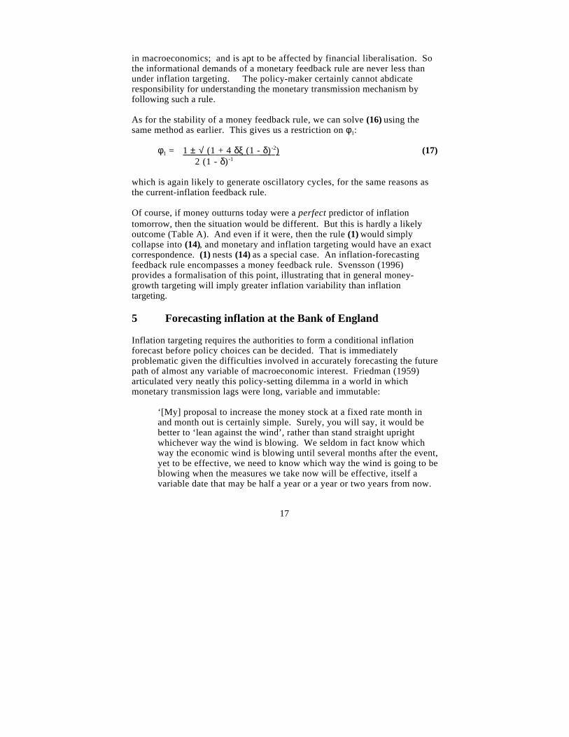
Chart 7 shows the intra-day response of implied sterling futures interest rateson six days - three corresponding to the release of the Bank’s Inflation Report ,and three corresponding to days on which Chancellor/Governor minutes werepublished. The time of publication is also shown. It is fairly clear that the‘news’ from these publications does indeed have an effect upon interest rateexpectations, as we might expect. (29) In some cases - for example, the May1995 Inflation Report , and the November 1994 and January 1995Governor/Chancellor minutes - the effects are sizable. This suggests,tentatively, that greater transparency may have raised unconditional assetprice variability on the day of news releases. These effects are usually small,however - for example, the February 1996 Inflation Report . And it is notaltogether clear that total unconditional variability has been raised bytransparency, aggregating across news and non-news release days.

To capture the conditional variance of asset prices, we looked at theforecasting error - or ‘surprise’ - in short-term interest rate expectations. Theevents we consider now are official interest rate changes in the period beforeand after the introduction of the United Kingdom’s inflation target regime. Sowe measure the interest rate ‘surprise’ for each official interest rate change,indexed k, as:

‘surprise’k = | i k,t - Ek,t -1 (i k,t ) | (20)

where the expectation of an official rate change is given by the previousday’s implied interest rate on the futures contract which is next to expire.(30)

We compare average interest rate surprises over two windows: March 1984-

(29) Haldane (1997) looks at the same evidence, for both short and long-term interest rateexpectations, averaged over a greater number of events, and finds the same patterns.(30) Clearly this is only a proxy. For example, the next expiring futures contract can cover interestrate expectations up to three months ahead. But as the mean time to expiry of the next contract is 11/2 months, whereas the maximum frequency of routine interest rate changes is one month, this isunlikely to be a big problem for our exercise.

31

May 1992 (covering 58 official rate changes); and October 1992- March1996 (covering eleven rate changes).(31) The latter period covers the inflationtarget regime.

Over the earlier sample, the average interest rate surprise was 55 basis points;whereas over the latter sample the mean is around 18 basis points. To controlfor the different average size of official rate changes over the two samples,we can look at the mean of the ratio of interest rate surprises to officialinterest rate changes over the two periods. This gives numbers of over 100%for the first sample, and of 34% for the second. The implication, then, fromboth pieces of evidence is that interest rate forecasting errors are around threetimes as large in the earlier period.(32) This is a striking difference. At leastsome of this can probably be put down to heightened transparency about theUK authorities’ monetary policy reaction function, including the publicationof the Bank’s Inflation Report; the scheduling of regular monthly monetarypolicy meetings; and the inflation target itself. (33)

How might we weight these competing - conditional versus unconditional -effects? First, as a practical matter, it seems that the unconditionalvariability effect is in many cases minor in comparison with the conditionalvariability effect. Second, as a theoretical matter, it is clearly conditionalmoments which affect real decisions - for example, through risk premia.Unconditional variability is merely reflecting the revelation of previouslyasymmetric information between private sector agents and the monetaryauthorities. Heightened unconditional variability

(31) We omit from both samples the three interest rate changes - on 16, 17, 22 September - around thetime of sterling’s exit from the ERM.(32) The 100% forecasting error in the earlier period seems large and so is its variance. It isaffected by several large surprises during periods when interest rates were being changed veryfrequently - for example, at the beginning of 1985. But stripping these out - which it is by no meansclear is optimal - would still give the same qualitative differences. The large variance also meansthat we are unable to reject the hypothesis that the mean surprises are not statisticallysignificantly different.(33) Haldane and Read (1997) find a significant stabilising effect of the inflation-targeting regimeon the whole of the interest rate term structure in the United Kingdom.

32

09.00 10.00 11.00 12.00 13.00 1 4 . 0 0 1 5 . 0 0 16.00 17.00 18.00

09.00 10.00 11.00 12.00 13.00 14.00 15.00 16.00 17.00 18.00

09.00 10.00 11.00 12.00 1 3 . 0 0 1 4 . 0 0 15.00 16.00 17.00 18.00

0 9 . 0 0 1 0 . 0 0 11.00 12.00 1 3 . 0 0 1 4 . 0 0 15.00 16.00 17.00 18.00

0 9 . 0 0 1 0 . 0 0 11.00 12.00 1 3 . 0 0 1 4 . 0 0 15.00 16.00 17.00 18.00

11 May 1995

(June 1995 futures contract)

15 June 1994

(September 1994 futures contract)

2 August 1995

(September 1995 futures contract)

16 November 1994

(December 1994 futures contract)

14 February 1996

(March 1996 futures contract)

11 January 1995

(March 1995 futures contract)

7.20

7.18

7.16

7.14

7.12

7.10

7.08

7.06

7.04

7.02

7.00

6.98

6.96

6.94

6.92

6.90

7.10

7.08

7.06

7.04

7.02

7.00

6.98

6.96

6.94

6.92

6.90

6.88

6.86

6.84

6.82

6.80

6.30

6.28

6.26

6.24

6.22

6.20

6.18

6.16

6.14

6.12

6.10

6.08

6.06

6.04

6.02

6.00

0 9 . 0 0 1 0 . 0 0 11.00 12.00 1 3 . 0 0 1 4 . 0 0 15.00 16.00 17.00 18.00

Per cent

Per cent

Per cent

Per cent

Per cent

Per cent

Inflation Report: selected publication dates Governor / Chancellor minutes: selected publication dates

Publ icat ion at 11.30 Publ icat ion at 09.30

Publ icat ion at 11.30 Publ icat ion at 09.30

Publ icat ion at 11.30 Publ icat ion at 09.30

Implied intra-day sterling interest rates

5.80

5.78

5.76

5.74

5.72

5.70

5.68

5.66

5.64

5.62

5.60

5.58

5.56

5.54

5.52

5.50

6.50

6.48

6.46

6.44

6.42

6.40

6.38

6.36

6.34

6.32

6.30

6.28

6.26

6.24

6.22

6.20

7.30

7.28

7.26

7.24

7.22

7.20

7.18

7.16

7.14

7.12

7.10

7.08

7.06

7.04

7.02

7.00

Chart 7

33

ought then to reduce conditional volatility over the long run, with beneficialeffects for information assimilation by agents and hence risk premia. By thismeasure, greater transparency has clearly had a net beneficial impact in theUnited Kingdom, and probably elsewhere too.

8 Does inflation targeting destabilise output?

One of the original arguments for monetary targets, dating back at least toFriedman (1959), was that they embodied an automatic cyclical stabiliser.So, for example, a supply shock which shifted prices and quantities inopposite directions would prompt an accommodating response from interestrates, which would remain (broadly) unchanged for fixed money supply. Thisis the correct response in the face of a shift in the equilibrium price level.Conversely, a demand shock would induce an interest rate response - forexample, raising interest rates following a positive money demand shock forfixed money supply - thereby heading off any effect on prices. So moneytargeting has a built-in cyclical stabiliser - in the absence of velocity shocks -ensuring the right policy response following both demand and supply shocks.The same automatic stabilisers in fact also operate with nominal GDP targets(Bean (1983), Hall and Mankiw (1994)).(34)

Inflation targets appear, on the face of it, to fare badly on these criteria. Theyinduce the correct policy response to demand shocks - a non-accommodatingone. But, narrowly interpreted and applied, they also imply non-accommodation of supply shocks - a suboptimal response. In effect, inflation-targeting in principle risks responding to one-time shifts in the price level, inaddition to trend inflationary disturbances.

In practice, this drawback has been overcome in two ways. First, through theuse of exemptions or caveats for certain supply shocks: whether explicitly -as, for example, under New Zealand’s Policy Targets Agreement where awide range of supply shocks are specified up front and then exempted if theyare ‘significant’; or implicitly - as in most other inflation-target countries.(35)

For example, in the United Kingdom the clearest example of supply shockaccommodation followed the rises in indirect taxes in 1993 and 1994. Thesetemporarily boosted measured inflation. At this time the UK authorities basedmonetary policy around an underlying inflation measure, which excluded

(34) More so, in fact, since money GDP targets are not susceptible to destabilising velocity shocks.(35) For example, the United Kingdom and Spain explicitly exclude only mortgage interestpayments from their headline measures; Canada exclude indirect taxes and food and energy pricesfor operational purposes; Australia exclude mortgage interest payments, government-controlledprices and energy prices; Finland exclude housing capital costs, indirect taxes and governmentsubsidies; while Sweden has no formal exemptions.

34

first-round indirect tax effects. In this way, the first-round effects of thesupply shock were effectively accommodated. A similar policy response wasrecently evident in other inflation-targeting countries subject to indirect taxrises, such as Spain and Sweden. With supply shocks accommodated in thisway, we would expect inflation targets to behave much like money GDP ormonetary targets as a cyclical stabiliser.

Second, the forward-looking nature of the reaction function under inflationtargeting helps prevent a policy response in the face of supply shocks. Price-level shocks should, in most circumstances, have only a temporary effect onmeasured inflation which washes out two or more years ahead - the horizon ofthe (forecast) feedback variable. (36) So following the forward-lookingfeedback rule, (1), ought to result in supply-shock accommodation and henceno unnecessary destabilisation of output.

Indeed, one can go further and argue that forward-looking inflation targetinggenerates explicit output stabilisation. This is true in two regards. First, theoutput gap is a key component of the inflation forecasting model, (18)-(19).So substituting for the expectation in (1) using (18)-(19) would give afeedback rule conditioned on the currently observed output gap, as well asother predetermined variables. Such a reaction function in fact looks quite alot like a Taylor rule, though it need not have equal or even similar weightson the inflation and output gap terms (see Svensson (1996)). Because of this,an inflation-targeting reaction function can be seen to imply explicitcountercyclical stabilisation. Clark, Laxton and Rose (1995) illustrate this ina simulation setting.(37)

Second, the extent to which policy is forward-looking can be thought todictate the relative weight placed on output versus inflation stabilisation.(38)

So the longer the lead, j, in the policy rule (1), the greater the implicit weightbeing assigned to output versus inflation stability. For example, at oneextreme monetary policy could aim to correct any deviation of expectedinflation from target as quickly as was technically feasible. But that wouldrisk a serious destabilisation of output. Lengthening the targeting horizon -smoothing out the transition path for inflation back to target - makes for asmoother output trajectory too. By judicious choice of j, the authorities cansecure the desired degree of output smoothing.

(36) Some supply shocks may be persistent. This persistence would then need to be taken intoaccount by the authorities when choosing the horizon for expected inflation from which to feedback.(37) Indeed, as Clark, Laxton and Rose (1995) illustrate, with a convex Phillips curve, minimisingthe variance of output increases the average level of output too.(38) Svensson (1996) provides a formalisation of this point.

35

Under the current UK policy framework, the Bank is required to declare, in anopen letter to the Chancellor, the horizon over which it expects inflation toreturn to target, should it deviate by more than 1 percentage point either side.The choice of an appropriate horizon will depend, among other things, on thesize of the initial inflation deviation from target and the source of the shockcausing it (demand versus supply). Such an institutional arrangementautomatically builds into the framework some degree of output stabilisation,allowing flexibility in the transition path of inflation back to target followingshocks.

9 Assessing the effects of inflation targeting

No country has much more than half a decade’s experience with inflationtargeting. With monetary transmission lags of two or three years, this blightsa quantitative evaluation of any ‘regime shift’ induced by the introduction ofinflation targets. But the qualitative evidence, at least, is broadlyencouraging.

Chart 8 plots inflation in New Zealand, Canada, Australia, the UnitedKingdom, Sweden, Finland and Spain. Also shown is the date their inflationtarget was first introduced.(39) Chart 9, meanwhile, plots (unweighted) averageinflation in these countries against (unweighted) average inflation in a controlgroup of low-inflation countries: France, Germany, the United States, Japanand Switzerland. Inflation is rising at the end of the period among theinflation targeters. But this largely reflects the more advanced stage of theseeconomies in the cycle. The really striking feature is the level at whichaverage inflation seems to be settling in these economies - which is nearer to1% than 5%.

Of course, the 1990s have been a period of global disinflation. So the chartsrisk confusing coincidence with causality. After all, inflation was on adownward path in many inflation target countries prior to the introduction oftheir targets. Further, the charts also tell us little about the output costswhich disinflationary transition has imposed. Or, put differently, they do nottell us whether inflation targets have secured any ‘credibility bonus’ bylowering inflationary expectations and, with them, the output costs ofdisinflation (see, for example, Blanchard (1984)).

(39) For Australia, this is taken (somewhat arbitrarily) to be January 1992.

36

(a) Consumer prices, except for the United Kingdom where RPIX was used.(b) Percentage increase in prices on a year earlier. Monthly data used, except for

Australia and New Zealand where data are quarterly.(c) It is difficult to date precisely the introduction of an inflation objective in

Australia as it has been gradually increased in importance over the past coupleof years. For the purpose of this exercise, however, we impose the pre/post inflation-target boundary at January 1992.

0 2 4 6 8101214

Sweden

012345678

Finland

0

2

4

6

8

10

12Spain

0

2

4

6

8

10Australia

Canada

0

2

4

6

8

10United Kingdom

0

4

8

12

16

20New Zealand

1985 86 87 88 89 90 91 92 93 94 95

+_

1 0 1 2 3 4 5 6 7

Inflation(a)(b)Chart 8

37

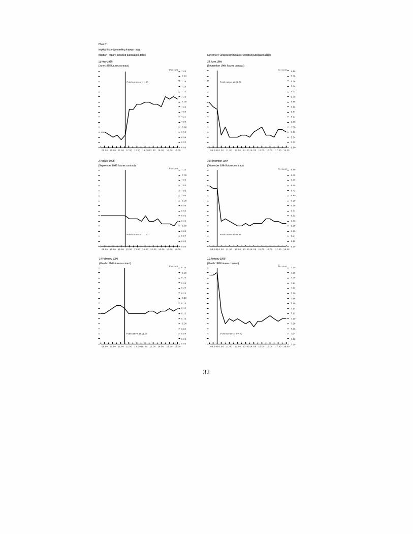
Table B reports some simple pooled summary statistics of (the mean andstandard deviation of) inflation and output among the set of inflation targeters(IT) and non-inflation targeters (NIT) used in Chart 9. For both sets ofcountries the sample is split: for ITs into the period before and after theintroduction of their targets; for NITs into the 1980s and the 1990s. Table Brepeats the message from Charts 8 and 9, with (mean/variance) inflationperformance now little different between the ITs and the NITs. At the sametime, neither the mean nor variance of output appears to have been greatlyaffected by the introduction of inflation targets in these countries - whetherlooked at over time or in the cross-section.

1985 86 87 88 89 90 91 92 93 94 95

0

1

2

3

4

5Percentage increase in prices on a year earlier

Average inflation: ITs versus NITs

Inflation targeters (a)

Non-inflationtargeters (b)

(a) United Kingdom, Canada, Sweden, Finland, Spain, Australia

and New Zealand.

(b) United States, France, Germany, Japan and Switzerland.

Chart 9

8

7

6

5

4

3

Per cent

0

1998 2000 05 10 15 20

30 September 1992

11 Apri l 1997

2 June 1997

UK forward inflation rates

Chart 10

38

Table BSummary statistics

Prior period(a) Post period(b)Inflation Output Inflation Outputµ σ µ σ µ σ µ σ

Inflation-targeting countries

8.1 1.9 2.1 0.6 2.7 1.0 2.3 1.0

Non inflation- targeting countries

4.3 2.1 2.5 0.7 2.8 0.8 2.1 1.4

(a) For the ITs, this covers the period from 1980 Q1 to the introduction of the target; for theNITs it covers the 1980s.

(b) For the ITs this covers the period from the introduction of the target to 1995 Q4; for theNITs it covers 1990 Q1-1995 Q4.

We can firm up these conclusions by conducting some simple tests of thedifferences in summary statistics. These are shown in Table C. Two featuresare striking. First, there is a significant difference in mean inflationperformance among the ITs before and after their targets were introduced.Further, the significant differences in mean inflation between the ITs andNITs in the prior period disappear in the latter period. Taken together, thisconstitutes reasonably strong evidence of a regime shift in the inflationperformance of the ITs, using either a time-series or cross-sectionalcounterfactual. Second, there is no evidence of the mean or variability ofoutput having been adversely affected by the disinflationary course that ITshave followed: for both sets of countries there is evidence of outputvariability having increased more recently; but this change is not statisticallysignificant and there is no evidence of the ITs having fared worse on thisfront.(40) Although it would be premature to argue that inflation targeting hasyielded a credibility bonus - lowering the output costs of disinflation byreducing inflation expectations - nor has it obviously levied a credibility tax. (40) Almeida and Goodhart (1996) do some very similar calculations based upon a different set ofcounterfactual countries - those with previously high inflation but which have not used inflationtargets as a disinflationary device. They find that these countries have performed at least as wellas the inflation targeters, providing prima facie evidence against inflation targets having hadmuch of an independent impact; or at least not one which is statistically discernable as yet. On thebasis of this and a comprehensive set of other diagnostic tests of various other macro variables,Almeida and Goodhart (ibid) conclude that the case for inflation targets is ‘unproven’, though it isstronger for countries (like New Zealand and Canada) with a longer track-record. Apart fromputting a bit of a gloss on some of the achievements of inflation targeters - for example, as regardstransparency, where Almeida and Goodhart (ibid) observe that the evidence is stronger - thispaper would not demur from those conclusions. Muscatelli and Tirelli (1996) estimate reactionfunctions for some OECD countries and find little evidence of a regime shift in the United Kingdomfollowing the adoption of an inflation target.

39

Table CTests of summary statistics

Inflation Output µ σ µ σ

ITs: prior and post periods 7.8 3.4 0.6 3.0NITs: prior and post periods -1.6 7.2(a) -0.5 3.4ITs v NITs in the prior period 3.3(a) 1.3 -1.0 1.8ITs v NITs in the post period -0.2 1.7 0.3 2.0(a) Denotes significance at 5%. The µ-test is a difference in mean test which is t-distributed with

n-1 degrees of freedom, where n is the number of countries. The σ-test is calculated as the ratio ofvariances which is F-distributed with (n, m) degrees of freedom, where n is the number of countriesin the variance of the numerator, and m the number of countries in the variance of the denominator.

Instead of looking at the reduced-form evidence, we might try inferringdirectly any regime shift in inflation expectations. The presence of an index-linked bond market in the United Kingdom offers a measure of inflationexpectations (see Deacon and Derry (1994)). Chart 10 presents someevidence on these; it plots the whole inflation term structure on three dates:immediately following the United Kingdom’s ERM exit; prior to theannouncement of operational independence for the Bank; and more recently.It suggests a pronounced downward shift in inflation expectations betweenSeptember 1992 and April 1997; and a further downward shift following theannouncement of the Bank’s operational independence.

Two possible explanations of these falls in implied inflation expectations arethat they are cyclically related or reflect a fall in the inflation risk premium.(41)

The first seems implausible. Chart 1 plots a ten-year forward inflation rate -a point expectation ten years hence - which should in principle beindependent of the cycle. This still shows the same fall-off in inflationexpectations. And as Chart 10 shows, the decline in inflation expectationshas been as evident at the long end of the inflation term structure as the shortend.

The bottom panel of Chart 1 provides a proxy for risk premia - the impliedvolatility embedded in options contracts on long-dated UK government bonds.This measure is little changed comparing the beginning and end of the

(41) A recent paper by Freeman and Willis (1995) considers these (and other) propositions inCanada, Sweden, New Zealand and the United Kingdom using bond yield data. They constructmeasures of real interest rates - something which we have side-stepped here by using the UKindexed bond market. They find some evidence of a rise in inflation expectations as these countrieshave emerged from recession; and some tentative signs of a fall in the risk premium.

40

periods, suggesting that the risk premium itself is potentially little changed.That leaves us tentatively concluding that the movements in Charts 1 and 10most likely reflect lower inflation expectations which have beenregime-induced. The charts also suggest that the level of measured inflationexpectations may still be too high to be consistent with the United Kingdom’sinflation target. Freeman and Willis (1995) find the same to be true inCanada, New Zealand and Sweden. This tells us that the process ofcredibility accretion has been gradual and is on-going. But because inflationtargeting is still in its infancy, this is not that surprising.

10 Conclusions

This paper has described some of the issues raised by inflation targeting ascurrently operated in the United Kingdom and elsewhere. Just as centralbanking has been described as an art, inflation targeting is inevitably a mix ofrules and discretion. But provided discretion is exercised subject to the rightset of incentives, and with a sufficient degree of transparency, this need notbe a cause for inflationary concern. After all, all science is rooted in someset of assumptions or priors. A Bayesian approach underlies monetarypolicy-making in all central banks, not just the inflation-targeters.

But even priors need scientific verification and testing. This is no trivial task.As Keynes observed:

‘...[A]n internal standard, so regulated as to maintain stability in anindex number of prices, is a difficult scientific innovation, never yetput into practice’ (Keynes, 1923)

Inflation-targeting countries have put into practice just such a scheme. Somehave perhaps made scientific innovations along the way - the Bank ofEngland’s published probability distribution perhaps being one of them. In thelong run, such technological innovations in the setting of monetary policyshould pay dividends.

41

References

Almeida, A and Goodhart, C A E (1996), ‘Does the Adoption of InflationTargets Affect Central Bank Behaviour?’, mimeo, London School ofEconomics.

Ammer, J and Freeman, R T (1995), ‘Inflation Targets in the 1990s: TheExperiences of New Zealand, Canada, and the United Kingdom’, Journal ofEconomics and Business, 47.

Andersson, K and Berg, C (1995), ‘The Inflation Target in Sweden’, inA G Haldane (ed), Targeting Inflation, Bank of England, London.

Astley, M S and Garrett, A (1996), ‘Interpreting Sterling Exchange RateMovements’, Bank of England Quarterly Bulletin, November, pages 394-404.

Bank of Canada (1994), Economic Choice and Policy Behaviour Under PriceStability, Bank of Canada.

Bean, C R (1983), ‘Targeting Nominal Income: An Appraisal’, EconomicJournal, 93, pages 806-19.

Bernanke, B S and Mihov, I (1996), ‘What Does the Bundesbank Target?’,NBER Working Paper No 5,764.

Blanchard, O J (1984), ‘The Lucas Critique and the Volcker Deflation’,American Economic Review, 74, pages 211-15.

Bowen, A (1995), ‘Inflation Targetry in the United Kingdom’, in A G Haldane(ed.), Targeting Inflation, Bank of England, London.

Brainard, W (1967), ‘Uncertainty and the Effectiveness of Policy’, AmericanEconomic Review, 57, pages 411-25.

Briault, C B, Haldane, A G and King, M A (1996), ‘Independence andAccountability’, forthcoming in Kuroda, I (ed), Toward More EffectiveMonetary Policy, proceedings of the Bank of Japan’s Seventh AnnualConference, October, 1995.

Britton, E and Whitley, J D (1996), ‘Asymmetry, Risks and the ProbabilityDistribution of Inflation’, mimeo, Bank of England.

42

Brunila, A and Lahdenpera, H (1995), ‘Inflation Targets: Principal Issuesand Practical Implementation’, in A G Haldane (ed), Targeting Inflation,Bank of England, London.

Bryant, R C, Hooper, P and Mann, C (1993), Evaluating Policy Regimes,The Brookings Institution.

Cechetti, S (1995), ‘Inflation Indicators and Inflation Policy’, NBER WorkingPaper No 5,161.

Clarida, R and Gertler, M (1995), ‘How the Bundesbank ConductsMonetary Policy’, mimeo, New York University.

Clark, P, Laxton D and Rose, D (1995), ‘Capacity Constraints, Inflation andthe Transmission Mechanism: Forward-Looking Versus Myopic PolicyRules’, IMF Working Paper No 75.

Cukierman, A (1995), ‘Towards a Systematic Comparison Between InflationTargets and Monetary Targets’, in Leiderman, L and L E O Svensson (eds.),Inflation Targets, CEPR.

Cukierman, A and Meltzer, A (1986), ‘A Theory of Ambiguity, Credibilityand Inflation Under Discretion and Asymmetric Information’, Econometrica,54, pages 1,099-1,128.

Deacon, M and Derry, A (1994), ‘Estimating Market Interest Rate andInflation Expectations from the Prices of UK Government Bonds’, Bank ofEngland Quarterly Bulletin, August, pages 232-40.

Dhar, S, Fisher, P G, Holland, A and Pain, D L (1995), ‘Interest RateEffects in the Bank of England’s Medium-Term Forecasting Model’, inFinancial Structure and the Monetary Policy Transmission Mechanism, Bankfor International Settlements.

Dotsey, M (1987), ‘Monetary Policy, Secrecy and Federal Funds RateBehaviour’, Journal of Monetary Economics, 20, pages 463-474.

Duguay, P (1994), ‘Some Thoughts on Price-Stability Versus Zero Inflation’,mimeo, Bank of Canada.

Duguay, P and Poloz, S (1994), ‘The Role of the Staff Economic Projectionsin Canadian Monetary Policy Formulation’, Canadian Public Policy, Vol XX,No 2, pages 189-99.

43

Flemming, J (1976), Inflation, Oxford University Press.

Fischer, A (1995), ‘New Zealand’s Experience with Inflation Targets’, inLeiderman, L and L E O Svensson (eds.), Inflation Targets, CEPR.

Fisher, I (1911), The Purchasing Power of Money, MacMillan.

Freedman, C (1994), ‘The Use of Indicators and of the Monetary ConditionsIndex in Canada’, Frameworks for Monetary Stability: Policy Issues andCountry Experiences, Balino, T J and Cottarelli, C (eds), Washington:International Monetary Fund.

Freeman, R T and Willis, J L (1995), ‘Targeting Inflation in the 1990s:Recent Challenges’, Board of Governors of the Federal Reserve System,International Finance Discussion Paper No 525.

Friedman, M (1959), A Program for Monetary Stability, Fordham UniversityPress, New York.

Friedman, B M (1975), ‘Targets, Instruments and Indicators of MonetaryPolicy’, Journal of Monetary Economics, 1, pages 443-73.

Goodfriend, M (1986), ‘Monetary Mystique: Secrecy and Central Banking’,Journal of Monetary Economics, 17, pages 63-97.

Goodhart, C A E and Vinals, J (1994), ‘Strategy and Tactics of MonetaryPolicy: Examples from Europe and the Antipodes’, Banco de EspanaDocumento de Trabajo No 9, 425.

Granger, C W J (1995), ‘Can We Improve the Perceived Quality ofEconomic Forecasts?’, mimeo, University of California at San Diego.

Haldane, A G (1995a), ‘Inflation Targets’, Bank of England QuarterlyBulletin, August, pages 250-59.

Haldane, A G (1995b), Targeting Inflation: A Conference of Central Banks onthe Use of Inflation Targets, Bank of England, London.

Haldane, A G (1995c), ‘Rules, Discretion and the UK’s New MonetaryFramework’, Bank of England Working Paper, No 40.

44

Haldane, A G (1997), ‘Designing Inflation Targets’, in P Lowe (ed),Monetary Policy and Inflation-Targeting, Reserve Bank of Australia.

Haldane, A G and Salmon, C K (1995), ‘Three Issues on Inflation Targets’,in A G Haldane (ed), Targeting Inflation, Bank of England, London.

Haldane, A G and Read, V (1997), ‘Central Bank Secrecy and the YieldCurve’, mimeo, Bank of England.

Hall R E and Mankiw, N G (1994), ‘Nominal Income Targeting’, inMonetary Policy, N G Mankiw (ed), University of Chicago (for NBER).

Jonung, L (1979), ‘Knut Wicksell’s Norm of Price Stabilisation and SwedishMonetary Policy in the 1930s’, Journal of Monetary Economics, 5,pages 459-96.

Keynes, J M (1923), A Tract on Monetary Reform, MacMillan.

King, M A (1994), ‘Monetary Policy in the UK’, Fiscal Studies, 15,pages 109-29.

King, M A (1996), ‘Direct Inflation Targets’, paper presented at thesymposium on ‘Gelpolitische in Europe’ held in Frankfurt, April 1996.

Leiderman, L and Svensson, L E O (1995), Inflation Targets, CEPR.

Longworth, D and Freedman, C (1995), ‘The Role of the Staff EconomicProjection in Conducting Canadian Monetary Policy’, in A G Haldane (ed),Targeting Inflation, Bank of England, London.

Lougani, P and Swagel, P (1995), ‘Supply-Side Sources of Inflation:evidence from OECD countries’, Board of Governors of the Federal ReserveSystem, International Finance Discussion Paper No 515.

Marshall, A (1887), ‘Remedies for Fluctuation in General Prices’, TheContemporary Review.

Mayes, D and Chapple, B (1995), ‘Defining an Inflation Target’, inA G Haldane (ed), Targeting Inflation, Bank of England, London.

McCallum, B T (1983), ‘On Uniqueness in Rational Expectations Models:An Attempt at Perspective’, Journal of Monetary Economics, 11,pages 139-168.

45

McCallum, B T (1995a), ‘Inflation Targeting in Canada, New Zealand,Sweden, the United Kingdom, and in General’, forthcoming in Kuroda, I (ed),Toward More Effective Monetary Policy, proceedings of the Bank of Japan’sSeventh Annual Conference, October.

McCallum, B T (1995b), ‘New Zealand’s Monetary Policy Arrangements:Some Critical Issues’, Reserve Bank of New Zealand Discussion Paper NoG95/4.

Muscatelli, V A and Tirelli, M (1996), ‘Institutional Change, InflationTargets and the Stability of Interest Rate Reaction Functions in OECDEconomies’, mimeo, University of Glasgow.

Neumann, M J M (1995), ‘Monetary Targeting in Germany’, forthcoming inKuroda, I (ed), Toward More Effective Monetary Policy, proceedings of theBank of Japan’s Seventh Annual Conference, October, 1995.

Nolan, C and Schaling, E (1996), ‘Monetary Policy Uncertainty and CentralBank Accountability’, Bank of England Working Paper No 54.

Reifschneider, D L, Stockton, D J and Wilcox, D W (1996), ‘EconometricModels and the Monetary Policy Process’, mimeo, Board of Governors of theFederal Reserve System.

Rodgers, P (1997), ‘Changes at the Bank of England’, Bank of EnglandQuarterly Bulletin, August, pages 241-47.

Schachter, A and Stokman, A C J (1995), ‘Interest Rate Policy of theDeutsche Bundesbank: An Econometric Analysis for 1975 to 1992’, DeEconomist , 143, No 4, pages 475-94.

Sargent, T J and Wallace, N (1975), ‘Rational Expectations, the OptimalMonetary Instrument and the Optimal Money Supply Rule’, Journal ofPolitical Economy, 83, pages 241-54.

Svensson, L E O (1995a), ‘The Swedish Experience of an Inflation Target’,in Leiderman, L and L E O Svensson (eds), Inflation Targets, CEPR.

Svensson, L E O (1995b), ‘Optimal Inflation Targets’, ‘Conservative CentralBanks and Linear Inflation Contracts’, mimeo, Institute for InternationalEconomics, University of Stockholm.

46

Svensson, L E O (1996), ‘Inflation Forecast Targeting: Implementing andMonitoring Inflation Targets’, mimeo, Institute for International EconomicStudies, Stockholm University.

Thomas, R S (1996), ‘Understanding Broad Money’, Bank of EnglandQuarterly Bulletin, May, pages 163-79.

Whitley, J D (1997), ‘Economic Models and Policy-making’, Bank of EnglandQuarterly Bulletin, May, pages 163-73.

Wicksell, K (1898), Interest and Prices, MacMillan.

Woodford, M (1994), ‘Non Standard Indicators for Monetary Policy: CanTheir Usefulness Be Judged From Forecasting Regressions?’, in N G Mankiw(ed.), Monetary Policy, University of Chicago Press, Chicago.

Yates, A (1995), ‘On the Design of Inflation Targets’, in A G Haldane (ed),Targeting Inflation, Bank of England, London.