Some Examples of Risk Analysis in

Environmental Problems - Keynote Talk ∗

David R. Brillinger, University of California, Berkeley

December 10, 2002

Abstract

Risk analysis, that is the problem of estimating the probabilities of rareand damaging events, unifies the geosciences. One can mention the risksfrom: floods, earthquakes, forest fires, space debris. The probabilities maybe fed into the computaion of insurance premiums. The Poisson processoften plays a prominent role, while marked point processes have a basicfunction. Various ways to collect and extrapolate data will be describedand examples from various fields will be presented. The topic unifies theenvironmental sciences.

1 Introduction.

1.1 Risk.

Risk may be defined as the probability of some hazardous event or catastrophe,the chance something bad will happen. In many cases huge amounts of moneyare involved [24]. The principal concern is low probability - high consequenceevents, events that lead to damage, loss, injury, death, environmental impair-ment for example. Often the work is done as an aid to decision making. Inconsequence risk models and risk management pervade modern technical life.

A common tool in the work is a catastrophe model. These have been definedas: a set of databases and computer programs designed to analyze the impact ofdifferent secenarios on hazard-prone areas [24]. In practice these models combinescientific risk assessments of the hazard with historical records to estimate theprobabilties of disasters of different magnitudes and the resulting damage toaffected structures. The information may be presented in the form of expectedannual losses and/or the probability that in a given year the claims will exceeda certain amount.

Risk analyses may be required by the government. The end result may bea rate rather than a probability. To cite a specific example a Core DamageFrequency (CDF) value of 10−4 per reactor year is the value endorsed by the

∗Supported by NSF Grants DMS 97-04739, DMS 99-71309 and DMS 02-03921.

1

Nuclear Regulatory Commission in a Staff Requirements Memorandum as abenchmark objective for accident prevention [26]. This rate is the probabilityof damage to a reactor core within a year. Its units may be viewed as numberof events per year. See [11].

The field of risk analysis cuts across the environmental sciences. Here wefocus on some geophysical risks, risks of things like: landslides, avalanches,earthquakes, floods, huricanes, tornadoes, forest fires, space debris, sea storms,and hail storms, ...

A formal risk analysis often includes: i) estimation of probabilities, ii) de-termination of the statistical distribution of damage and iii) preparation ofproducts like formulas, graphics, hazard risk maps. There is extensive use ofcomputing science, substantive subject matter and statistical methods.

A pair of revealing examples are provided by the papers of Fairley, [12], andMiller and Leslie, [21]. The Fairley work is concerned with the probability of aspill of liquified natural gas during its importation at U.S. ports. In particularthe paper makes the case for describing risks by probabilities not by their recip-rocals i.e. return periods, ( the mean interval between events). The Miller-Lesliepaper concerns the probability of a ship hitting the Tasman Bridge at Hobart,Austalia. In both these papers there is careful evaluation of the probabilities ofcomponent events.

1.2 Some basic concepts.

The tools of risk analysis include: statistical methods, substantive background,computer software and hardware. The products include probability estimates,hazard maps, decisions.

Among the pertinent statistical concepts are: borrowing strength, forecast-ing, (marked) point processes, Bayes Theorem, influence diagrams, uncertaintyestimation, distributions, models (extreme value, threshold, Poisson, binary re-sponse, nonparametric and nonparametric methods).

Ideas from systems analysis and computing science also prove extremely use-ful in risk analyses. These include: box and arrow diagrams, software packages,simulation, decision tools, GIS, visualization, and data base management.

Both statistics and computer science often adopt the strategy of breakingthe problem down conceptually.

2 Some examples of risk analyses.

2.1 Example 1 - Amazon Floods.

The first example concerns the risk of floods on the Amazon River. A renewalmodel is employed for the times of events, in part because the data set is small.

2

Manaus is a city well up the Amazon in Central Brazil. At a dock theriver’s height has been recorded daily since 1903. Also there are newspaperrecords and journals that may be consulted to determine the dates of someearlier floods. [31]. Of official concern is the question of whether the risk offlooding is increasing. Increased flooding will eventually occur because of thedeforestration taking place ibid.

The top panel of Figure 1 provides the dates of floods. There were 21 of themduring the period 1892 to 1992. The definition take for a flood, when specificmeasurements were available, was that the stage exceeded 28.5m. In the panelthe dates are indicated by points along the x-axis and points of increase in thecumulative count function N(t). To estimate the hazard function one needs adistribution function for the times between events. The histogram of the timesbetween successive floods is given in the middle panel of Figure 1. The longtail suggests the use of a Pareto distribution with p.m.f. p(u) = Cα/uα, u =1, 2, 3, ... . The domain is integers because the data employed are years. Thecurve fit by maximum likelihood is superimposed in the second panel. It isassumed that the times bewteen events are independent, i.e. the point processis renewal.

The bottom panel provides an estimate of the hazard as a function of timesince the last year of the data employed in our analysis, 1992. Approximate90% confidence intervals are also indicated. These were obtained by workingwith the logit transform and employing the delta-method.

More details of the analysis may be foiund in the papers [31], [3].

2.2 Example 2 -Great Earthquakes in California.

The concern of this example is probabilities for future great earthquakes inSouthern California. Once again a renewal process is employed, i.e. the timesbetween events are assumed i.i.d..

Pallett Creek is a location northeast of Los Angeles that is astride the SanAndreas Fault.. It has interesting geological structure. In the early eightiesthe paleogeologist Kerry Sieh dug a trench that crossed the San Andreas Faultthere [29]. The trench showed an interesting structure - a number of sedimentarylayers were visible. There were breaks in the layers and Sieh inferred that thesewere due to great earthquakes. For most of the breaks he was able to collectsamples of material that could be dated by radiocarbon (RC) methods. Siehcarried out further studies. The estimated dates of earthquakes whose presencehe inferred are shown in Figure 2.

The analysis here is interesting for: the small number of data points involved,the presence of a missing value, an open interval and substantial measurementerror. In order to obtain estimates of risk a renewal process with a Weibulldistribution is hypothesized for the intervals between the events. The Weibull

3

1892-1992 Manaus floods (> 28.5m)

year

1900 1920 1940 1960 1980

5

10

15

20

• • • • • • • • • • • • • • • • • • • • •

0 5 10 15 20

0

1

2

3

4

5

6

Intervals between floods - discrete Pareto fit

years

coun

t

Probability of flood in u years from 1992

approximate 90% CI’su, years from 1992

prob

abili

ty

0 5 10 15 20 25 30

0.0

0.2

0.4

0.6

0.8

1.0

Figure 1: Panel 1 is a step function counting the number of floods since Jan-uary 1892. The dashed line’s slope provides the rate of events. Panel 2 is thehistogram of the intervals between floods and a fitted Pareto. Panel 3 is theestimate of the hazard function and approximate 90% confidence intervals.

4

density is

Probinterval ≤ x = 1 − exp−(x/α)β−1, x > 0

Measurement error from the radiocarbon dating is modelled as additive normalwith mean 0 and s.d. estimated at the RC laboratory. The missing date for anevent meant taking one of the available intervals as the sum of two Weibulls.The open interval starts at the last event. It occurred in 1857. Numericalintegration was employed to determine the density of a Weibull plus an inde-pendent normal and the one for the sum of two Weibulls. The reasonablenessof the Weibull assumption was assessed by the Weibull hazard plot given asthe middle panel of Figure 2. Maximum likelihood analysis was employed toestimate the parameters. More details may be found in [30].

The bottom panel of Figure 2 gives the estimated risk as a function of yearsinto the future from 1988. The figure also includes approximate 95% marginalconfidence bounds.

2.3 Example 3 - Earthquake Damage.

Cornell [10] is the seminal paper on seismic risk assessment (SRA). His definitionof the subject is a variant of the following:Seismic risk assessment - the process of estimating the probability that certainperformance variates at a site of interest exceed relevant critical levels within aspecified time period as a result of nearby seismic events.

The approach presented here is one of breaking the problem down concep-tually into manageable parts: a) damage, b) site, c) attenuation and d) eventlocations, times and sizes. These parts are illustrated in Figure 3.

In computing risks generally and seismic risks particularly two probabilityresults are basic:Bayes Rule

P (ABC...) = P (A)P (B|A)P (C|AB)...(1)

Total probability theorem

P (A) =∑

k

P (A|Bk)P (Bk)(2)

[34] is another fundamental paper. Figure 3 shows the corresponding series andparallel structure for two possible events.

In the presentation we work backwards from a structure at a site to thelocations, times and sizes of earthquakes. (Two events are illustrated in theFigure.)a) Damage. There are a variety of ways to describe and estimate damage. Animportant method uses the Modified Mercalli Intensity (MMI). One reason forits importance is that values may be derived from historic accounts. Another isthat it refers to damage directly.

MMI values are given by roman numerals I to XII (and sometimes 0 referringto no impact.) The scale is ordinal increasing with increasing severity of damage.

5

• • • • • • • • • •

Large earthquakes at Pallett Creek, CA

500 1000 1500 2000

•

• •

•

••

•

Cumulative Weibull hazard plot

cumulative hazard

inte

rval

, yea

rs

0.5 1.0

10

100

1000

4463 63

134200

246332

Probability of major fault rupture

u, years into future from 1988

prob

abili

ty

0 20 40 60 80 100

0.0

0.2

0.4

0.6

0.8

1.0

Figure 2: Panel 1 estimated dates of the Pallett Creek events; panel 2 Weibullhazard plot with the vertical lines indicating twice the RC dating s.e.’s; bottompanel the estimated risk. 6

Source1

Medium1

geometry

Source2

Medium2

Site

Structure

A_j>A?

(t_j,A_j)

dynamic responseresistivitynoise

geologyground typenoise

?

distanceattenuationgeophysicsnoise

noisetectonicslocationssize

Figure 3: Box and arrow diagram highlighting components of an SRA. Aj refersto the level of some performance variate occurring with the j-th event. A is athreshold level at which damage occurs.

7

For example the definition of MMI VIII includes: ”Damage slight in speciallydesigned structures; considerable in ordinary substantial buildings; ...” [7].

There are values that have been proposed to convert MMI values into damagepercentages for different types of structures. The following is an example of aso-called damageability matrix given in [23]. The entries are loss ratios per riskcategory in %.

MMI VI VII VIII IX Xresidential .4 1.7 6 17 42commercial .8 3 11 27 60industrial .1 .7 3 11 30

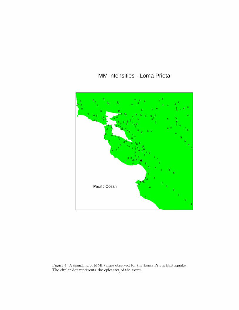
Figure 4 shows some of the MMI-values obtained following the Loma Pri-eta event of 17 October 1989. Th two large bays are San Francisco Bay andMonterey Bay. Only some of the observations are plotted to avoid overstriking.The epicenter of the event was near Santa Cruz California. (Arabic numeralsare plotted rather that Roman for convenience.) See also [32].

Next we seek a spatial distribution for the MMI values. Ordinal data areconveniently handled by postulating the existence of a latent variable ζ and cutpoints ai such that the MMI value at location (x, y) is given by

Ix,y = i if ai < ζx,y ≤ ai+1

Continuing we postulate a model

ζx,y = fx,y + εx,y

with fx,y deterministic and smooth and with εx,y having an extreme value distri-bution. The use of the extreme value distribution is plausible given the nature ofdestruction. It and the corresponding cloglog link mean that the function glm()may be used for the computations, see McCullagh and Nelder [20], Chapter 5.

In [5] fx,y is estimated using the generalized additive models fitter gam() ofHastie and the smoother loess() of Cleveland [9], on data from the Loma Prietaevent employed. Figure 5 provides the estimate of f . One see a general dyingoff of the function values as one moves away from the epicenter, except for arise near San Francisco. This increase is associated with reclaimed land.

b) Attenuation. Next a relationship describing the fall-off in energy with dis-tance as it passes through the medium is needed. This general fall-off is apparentin Figure 4. Following Joyner and Boore, [17], consider the attenuation form

log(−log(1 − ProbI = i)) = αi + βd + γlog(d) + δM(3)

where d is the distance of the observation point to the epicenter of the eventand M the event’s magnitude. This was fit to the Loma Prieta data. (As onlyone event was involved δ could not be estimated separately of the αi.). Theresults are given in Figure 6. In the case of MMI VIII one sees a very rapidfall-off with distance.

8

MM intensities - Loma Prieta

Pacific Ocean

•

5

5

45

5

5

6

6

5

5

6

55

4

6

6

66

6

6

679

66

46

77

7

77

779

77

7

6

77

6

7 67

66

6

56

6

7

677

56

76

77

76

6

6

8

77

6

7

66

6

87

8

6

6

66

6

66

5

5

8

8

78

66

5

7

66

5

6

7

87

66

6

6

6

6

5

5

6

7

6

6

6

6

5

5

3

6

666

8

6

66

6

4

6

7

8

66

6

6

6

55

5

7

7

7

5

55

7

7

6

4

6

6

4

4

6

8

6

5

4

5

6

6

6

5

5

4

4

6

5

5

4

5

6

4

6

5

5

4

4

5

4

0

5

6

Figure 4: A sampling of MMI values observed for the Loma Prieta Earthquake.The circlar dot represents the epicenter of the event.

9

Loma Prieta event: estimated surface

longitude

latit

ude

-123.0 -122.5 -122.0 -121.5 -121.0

36.0

36.5

37.0

37.5

38.0

38.5

Pacific Ocean

•

-4

-4

-3

-3

-3

-2

-1

-1

0

0

1

Figure 5: The estimate of the surface fx,y.

10

Loma Prieta prob I = i | source distance

distance (km)

prob

abili

ty

0 200 400 600

0.0

0.2

0.4

0.6

0.8

1.0

VIII

V

O

Figure 6: Fitted probabilities of the indicated MMIs as a function of distancefrom the epicenter.

c) Event locations and times. One imagines a marked spatial-temporal pointprocess of earthquake locations, times and sizes, (xi, yi, ti, Mi). In Californiamany faults have been located. In Figure 3 just two sources have been hypoth-esized, but there could be many. One uses the total probability theorem (2).In an expression like (3) one might take d to be the distance to the nearestpoint on the fault from the site. Faults have been modelled as line and planesegments with event magnitude related to their size. There are many geologicalfault maps to work with.

Commonly renewal processes are employed to model the sequence of times.The intervals between events might be assumed exponential, Weibull or lognor-mal.

As an example of a fair premium computation, consider a commercial build-ing 25km from an epicenter and an event like Loma Prieta. For this case theestimated expected loss is

.8 ∗ .102 + 3 ∗ .389 + 11 ∗ .475 = 6.47%

and so the fair premium would be 6.47% of the amount insured.See [2] for further details concerning this example.

2.4 Example 4 - Forest Fires.

In this example we turn to the problem of predicting the occurrence of forest firesas a function of place and time. Let occurrences be denoted by (xj, yj, tj), j =1, 2, 3, ... . One has a point process in space and time.

11

Km

Km

0 200 400 600

010

020

030

040

050

060

0

Elevation map and 1990 Federal fire locations

Figure 7: Locations of fires in Oregon during 1989-1996

To illustrate the idea consider Figures 7 and 8. Figure 7 shows the locationsof forest fires in Oregon during the period 1989-1996 that occurred in Federallands. These lands are indicated in Figure 8.

Consider voxels (x, x + dx]× (y, y + dy] × (t, t + dt] and let

Nx,y,t = 1 if a fire in the (x, y, t) voxel

= 0 otherwise

For convenience suppose that dx, dy, dt = 1. (In the data and computationsdx, dy = 1km and dt is 1 day. Letting Ht denote the history of the processup to time t, consider the probability

ProbNx,y,t = 1 | Ht = px,y,t

In the work a logit model was assumed, specifically

logit px,y,t = g1(x, y) + g2(d) + ζ

with (x, y) - location, d - day of the year, ζ year effect. The g functions areassumed to be smooth in the computations and are represented by spline func-tions. The spatial term, g1, involved a thin plate spline and the day term, g2,was a spline with period one year. The function took the form

g1(x, y) = α + βx + γy +J∑

j=1

δjr2j log rj

12

Km

Km

0 200 400 600

010

020

030

040

050

060

0

Federal lands mask

Figure 8: Federal lands in Oregon

where for nodes (xj, yj) the distance is r2j = (x − xj)2 + (y − yj)2, [27]. The

Splus function make.rb() of Funfits, [13], was employed in the computations.Logit models have been used previously in estimating fire risk, see for example[19].

The data set for Oregon was very large, 578,192,400 voxels and 15,786 fires.To be able to carry out exploratory data analyses a sample of the data used.All the voxels with fires were employed, but only a sample of those where nofires occurred. The sampling fraction was π = .00012 This lead to 58094 casesfor the analysis.

With the logit link, conditional on the sample one had a generalized linearmodel (glm) with an offset of log 1/π. This meant that standard glm computerprograms could be used for the analysis. (The new logit was logit p′ = logit p + log(1/π).)

The results are provided in Figure 9. One has estimates of the functionsg1, g2 and the effects ζ. The ζ are assumed fixed, but in work in progressthey are random. Examining the top panels one sees fewer fires in SE Oregon,as could have been anticipated from Figure 7. In the thin-plate computations60 nodes were employed and they were taken to be 10km apart throughoutthe region. From the bottom left panel of Figure 9 one notes a definite dayeffect - more fires in the summer. From the bottom right panel there appearsto be a definite year effect. The year effect values are relative to 1996 as 0.The horizontal line is at 0. Also in the bottom panels of the figure are ±2 s.e.bounds.

One can get estimated probabilities for a nominated region and times by

13

0200

400600

km 0

100

200

300

400

500

km

-6-5

-4-3

-2-1

Z

km

km

0 200 400 600

0

100

200

300

400

500

600

-5

-5

-4

-4

-4

-3

-3

-3

-3-2

Day effect

day

0 100 200 300

-12

-10

-8

-6

Year effects

year

1990 1992 1994 1996

-0.4

-0.2

0.0

0.2

0.4

0.6

0.8

•

Figure 9: Top panels - estimated location effect, g1 in perspective and coutourform. Bottom left panel - estimated day effect. Bottom right panel - estimatedyear effects. Approximate 95% error bounds are indicated.14

Estimated mean rate for Umatilla Forest

+- 2 s.e. boundsday

rate

(fir

es/k

m-s

quar

ed)

0 100 200 300

0.0

0.2

0.4

0.6

0.8

1.0

1.2

1.4

Figure 10: Estimated rate of fires (fires/km-squared/day) for the Umatilla For-est region.

adding voxel values. This is done for the Umatilla Forest and the results arepresented in Figure 10. (This region is the green area within the rectangle ofFigure 8. Also in the bottom panels of the figure are ±2 s.e. bounds.). Thecount of fires in the region will be approximately Poisson following the Hodges-Le Cam result [14]. This may be used to obtain estimated probabilities of, forexample, the number of fires in a specified time period exceeding a specifiedcount.

The above results are elaborated upon in [6], [28]. Currently the work isinvolving other explanatories, random year effects and extensions to other statesof the U.S. . An example of a meteorological variable is moisture level, see Figure11.

2.5 Example 5 - Space Debris.

The space near the Earth has been described as a veritable garbage can. Thereare now in orbit millions of pieces of debris. These result from space activitiesover the last 45 years. More than 200,000 of the pieces are between 1 and 10cmin size. They orbit at speeds of several kilometers per second and can causesubstantial damage if they hit another object. In designing shielding for a spaceobject it is important to know the risks of collisions, [25], [15], [1].

An example of a question that arises is: What is the chance of some 1-10 cmpiece of debris passing through the 11000m2 cross-section of the InternationalSpace Station space in the next 15 years? We will consider a simple variant.

There is considerable scientific knowledge of the physics of orbits dating backto Kepler and Newton, see [33]. It may be used to estimate risks, [16], [8], [18].

15

Figure 11: Moisture level for a week in July 1994

16

Figure 12: A three dimensional representation of the orbit of an object showingthe elliptical orbit in the plane of rotation.

Figure 12 is taken from the NASA site www-istp.gsfc.nasa.gov/stargaze/Smotion.htm. It shows the character of orbits and sets up some notation. In the figure: X isthe direction to the Vernal Equinox, N is the direction of the Ascending Node,Ω is the Right Ascension, P is the point of Perigree, i is the inclination, ω isthe argument of Perigee . A basic aspect of the motion of an orbiting object isthat it takes place in a plane and is elliptical, [33] and [22]. This is illustratedin the Figure.

For the moment considerations and notation are restricted to the case ofthe plane. Figure 13 shows a quarter of an orbit. The Earth is at the focus,O, and at time t the object is at P which will be described by (ft, rt) usingpolar coordinates with ft, the true anomaly. A related angle is Et, the eccentricanomaly. These variables are illustrated in Figure 13. The elliptical orbit maybe represented as

rt = a(1 − e cos Et)

where a is the semimajor axis and e the eccentricity of the ellipse. The ellipseis swept out as Et varies. In terms of Figure 13 the object is at (φt, rt) whereφt = ω + ft.

The equations of motion may now be written

cos ft = (cos Et − e)/(1 − e cos Et),

sin ft =√

1 − e2sin Et /(1 − e cos Et)

17

••

•

••

E fO

P

Figure 13: The solid line represents a quarter of an orbit. The point O, the focusof the ellipse, represents the Earth. The point P is the position of the object onits orbit. The angle f is the true anomaly. The angle E is the eccentric anomaly.The dashed line is the circumscribing circle.

18

n(t − T ) = Et − e sin Et

The last is Kepler′sEquation. The constant n is the mean motion and P = 2π/nis the period.

The paper [4] considers the rate of objects passing through a patch of spaceand develops results using traditional statistical methods. Previous researchershad used ergodic arguments in most part. In this 2-dimensional case a patch isdefined, in polar coordinates, by

(φ = a(u), r = b(u)), u ε U(4)

It is shown in [4] that the expected rate of objects passing through the patch is∫

E

∫U

p

(a(u) − atan(

√1 − e2sinE, cosE − e), t − 1

n(E − esinE)

)δ (a(1 − cosE) − b(u))

·|a′(u)aesinE − b′(u)√

1 − e2

1 − ecosE| du dE(5)

where p(ω, T ) represents the joint density of ω and T and δ is the Dirac deltafunction.

Consider the particular case of a line segment poining directly at O. It maybe represented by φ = φ0, r = r0 + u with 0 < u < ε. Suppose that ωis uniform on (0, 2π) and independently T is on uniform (0, P ), i.e. the initialconditions are random. The rate function is then

a√

1 − e2

r0

1√(r0 − q)(q′ − r0)

ε

πP(6)

where q, q′ = a(1 − e), a(1 + e), q < r < q′, 0 ≤ φ < 2π. This quantity doesnot depend on t, nor does it depend on φ0, as could have been anticipated. Thefunction is graphed in Figure 14 for the case of eccentricity .6 . The functiondepends strongly on r. One sees higher rates at the extremes, q, q′, of the orbitwith the highest at q.

In reality there are many orbiting objects. Their effects are superposed.They, i.e. their initial conditions, may be independent or they may be dependentas they result from the same breakup.

There are also important explanatories, such as solar pressure, drag, to in-clude in a model.

3 Discussion and Conclusions.

The demand for risk analyses is growing generally, in part because costs ofreplacing destroyed structures are growing and in part because of the steadyincrease in the population living in hazardous areas. Statistical methods arebasic to risk assessments. This is obvious because probabilities and data are

19

radial distance

inte

nsity

0.4 0.6 0.8 1.0 1.2 1.4 1.6

2

4

6

8

10

12

14

16

Figure 14: The rate function (6).

involved. It is also the case because statistics adds important things to whatthe engineers and scientists tend to know and do on their own. Statisticians addthings like efficiency results, extensions to different data types, and uncertaintyanalyses.

What have we learned from the examples presented? There are difficultiesand opportunities. There are solutions and there are lots of open problems. Thestochastic approach is highly effective.

What do the 5 examples have in common? - They are seeking probabilitiesand distributions. What do the solutions have in common? - Data and subjectmatter are basic. What are the products for each example? - Estimated prob-abilities. Which methods play an important roles? - Stochastic modelling andCI construction.

Acknowledgments.

Collaborators are basic to work on problems of the type considered. Mineinclude: Floods - Hilgard O’R. Sternberg, Great earthquakes - Kerry Sieh;MMI - Chiann Chang, Pedro Morettin, Rafael Irizarry; Fires - John Benoit,Haiganoush Preisler; Space debris - Abdel El-Sharaawi and the researchers atJohnson Space Center.

People who provided help concerning the computing includied Doug Bates,Chong Gu, Trevor Hastie and Phil Spector.

Part of the material was peresented in the keynote talk presented at the 2002Interface Meeting in Montreal. I thank Ed Wegman for the invitation.

20

References

[1] BARTON, D. K., BRILLINGER, D. R., EL-SHAARAWI, A. H., MCDANIEL, P., POL-LOCK, K. H. and TULEY, M. T. (1998). Final Report of the Haystack Orbital DebrisData Review Panel. Johnson Space Center, Tech. Mem. 4809.

[2] BRILLINGER, D. R.(1993). Earthquake risk and insurance. Environmetrics 4, 1-21.

[3] BRILLINGER, D. R. (1994). Trend analysis: time series and point process problems.Environmetrics 5, 1-19.

[4] BRILLINGER, D. R. (2001). Space debris: flux in a two dimensional orbit. Pp. 105-116 in Statistics and Genetics in the Environmental Sciences. (Eds. L. T. Fernholz, S.Morgenthaler and W. Stahel). Berkhauser Verlag, Basel.

[5] BRILLINGER, D.R., CHIANN, C., IRIZZARY, R.A. and MORETTIN, P.A. (2001).Automatic methods for generating seismic intensity maps. Probability, Statistics andSeismology: Journal of Applied Probability Vol. 38A, 189-202.

[6] BRILLINGER, D. R., PREISLER, H. K. and BENOIT, J. W. (2003). Risk assessment:a forest fire example. In press.

[7] BULLEN, K. E. and BOLT, B. A. (1985). An Introduction to the Theory of Seismology,Fourth Edition. Cambridge, Cambridge.

[8] CLEGHORN, G. E. A. (1995). Orbital Debris: a Technical Assessment. NationalAcademy Press, Washington.

[9] CLEVELAND, W. S., GROSSE, E. and SHYU, W. M. (1992). Local regression mod-els. Pp. 309-376 in Statistical Models in S. (Eds. Chambers, J.M. and Hastie, T.J.).Wadsworth, Pacific Grove.

[10] CORNELL, C. A. (1968). Engineering seismic risk analysis. Bull. Seismol. Soc. Amer.58, 1583-1606.

[11] ELLINGWOOD, B. (1994), Validation of Seismic Probabilistic Risk Assessment of Nu-clear Power Plants. U. S. Nuclear Regulatory Commission, GPO Washington.

[12] FAIRLEY, W. B. (1977). Evaluating the “small” probability of a catastrophic accidentfrom the marine transportation of liquefied natural gas. Pp. 331-354 in Statistics andPublic Policy (Eds. W. B. Fairley and F. Mosteller). Addison-Wesley, Reading.

[13] FUNFITS (2002). www.cgd.ucar.edu/stats/Software/Funfits

[14] HODGES, J. L. and LE CAM, L. M. (1960). The Poisson approximation to the PoissonBinomial distribution. Ann. Math. Statist. 37, 737-740.

[15] JOHNSON, N. L. (1998). Monitoring and controllingdebris in space. Scientific American62-67.

[16] JOHNSON, N. L. and MCKNIGHT, D. S. (1987). Artificial Space Debris. Orbit BookCo., Malabar.

[17] JOYNER, W. B. and BOORE, D. M. (1981). Peak horizontal acceleration and velocityfrom strong-motion records including records from the 1979 Imperial Valley, California,earthquake. Bull. Seism. Soc. Amer., 71, 2011-2038.

[18] KESSLER, D. J. (1981). Derivation of the collision probability between orbiting objects:the lifetimes of Jupiter’s outer moons. Icarus 48, 39-48.

21

[19] MARTELL, D. L., Otukol, S. and Stocks, B. J. (1987). A logistic model for predictingdaily people-caused forest fire occurrence. Canadian J. Forest Research 19, 1555-1563.

[20] MCCULLAGH, P. and NELDER, J. A. (1989). Generalized Linear Models, Second Edi-tion. Chapman and Hall, London.

[21] MILLER, A. J. and LESLIE, J. S. (1979). The risk of collisions between ships andbridges. Proc. 42nd Session of the ISI 48, 137-148.

[22] MONTENBRUCK, O. and GILL, E. (2000). Satellite Orbits. Springer, Berlin.

[23] MUNICH RE (1991). Insurance and Reinsurance of Earthquake Risk. Munich Re, Mu-nich.

[24] NATIONAL ACADEMY OF SCIENCE (1998). Paying the Price. (Eds. H. Kunreutherand R. J. Roth.) J. Henry Press, Washington.

[25] NATIONAL RESEARCH COUNCIL (1997). Protecting the Space Station from Mete-oroids and Orbital Debris. NRC, Washington.

[26] NUCLEAR REGULATORY COMMISSION (1997). Federal Register: June 25, 1997,Volume 62, Number 122 Notices 34321-34326.

[27] POWELL, M. J. D. (1992). The theory of radial basis function approximation in 1990.Advances in Numerical Analysis, Vol II. (Ed. W. Light). Oxford, Oxford.

[28] PREISLER, H. K., BRILLINGER, D. R., BURGAN, R. E. and BENOIT, J. W. (2003).Probability based models for the estimation of wildfire risk. Submitted.

[29] SIEH, K. E. (1984). Lateral offsets and revised dates of large prehistoric earthquakes atPallett Creek, Southern California. J. Geophysical Res. 89, 641-647.

[30] SIEH, K., STUIVER, M. and BRILLINGER, D. R. (1989). ”A more precise chronologyofearthquakes produced by the San Andreas Fault in Southern California,” J. GeophysicalResearch 94, 603-623.

[31] STERNBERG, H. O’R. (1987). Aggrevation of floods in the Amazon River as a conse-quence of deforestration? Geografiska Annaler 69A, 201-219.

[32] STOVER, C.W., REAGOR, B.G., BALDWIN, F. and BREWER, L. (1990). Prelim-inary Isoseismal Map For the Santa Cruz (Loma Prieta), California, Earthquake ofOctober 18, 1989. UTC: Open File Report 90-18. National Earthquake InformationCenter, Denver.

[33] SZEBEHLY, V. G. (1989). Adventures in Celestial Mechanics. University of Texas Press,Austin.

[34] VERE-JONES, D. (1973). The statistical estimation of earthquake risk. New ZealandStatistician 8, 7-16.

22