Some consistent finite element formulations of 1-D beam models: a comparative study

J. M. Ortuzar & A. Samartin

A consistent Finite Element formulation was developed for four classical 1-D beam models. This fo rmulation is based upon the solution of the homogeneous differential equation (or equations) associated with each mode l. Results such as the shape functions, stjffness matrices and consistent force vectors for the constant section beam were found. Some of these results were compared wilh the corTespooding ones obta ined by the standard Finite Element Method (i.e. using polynom ial expansions for the fie ld variables).

Some of the difficulties reported in the literature concerning some of these models may be avo ided by this technique and some numerical sensitivity analysis on this subject are presented.

Key words: finite element formulation, differential equations, polynomial functions.

1 INTRODUCTION

Piecewise polynomial functions were extensively used to express the expansion of the field variables in the Fini te Element Method. 1 However, this app roach, in the stmctural analysis, p resents some difficulties even in simple 1-D elements when shear strain is incl uded.2

An alternative to the use of polynomial functions is to consider the solution of the boundary value field problem. Some inconsistencies described in the previous reference about the formulations developed in the references' 6 can be in this way overcome. In some of those fom1ulations, overstiff solutions for long slender beams were obtained (shear locking); iu some cases more than two nodes per element were used, or, in other cases, on ly two nodes were required, but with more than two degrees of freedom at each node; in all those formul ations a significant number of elements was required to accurately represent the beha­viour of sh01t beams under complex distributions of the load.

Here, the previously mentioned alternative is applied to the following four beam models and in some or them the

results are compared with the standard FEM solutions:

I. Navier- Bem oulli beam model 2. Timoshenko beam model, i.e., shear strain included 3. Beam- column model 4. Beam- column model considering shear strain.

The notati on used in Sections 2-7 is given in Appendix A. The abscissa ~ of the beam element is defined along an element length L = I, i.e. ~ E [0, I]. Other variables related to the beam of unitary length are denoted by an overline. However, for sake of clarity in the figures the overline was dropped. The properties (bending and shear stiffncsses, El and GA respectively) are functions of the abscissa ~.

This study can be easily extended to a beam of arbitrary length L according to Appendix A.

2 NA VI ER- BERNOULLI BEAM MODEL

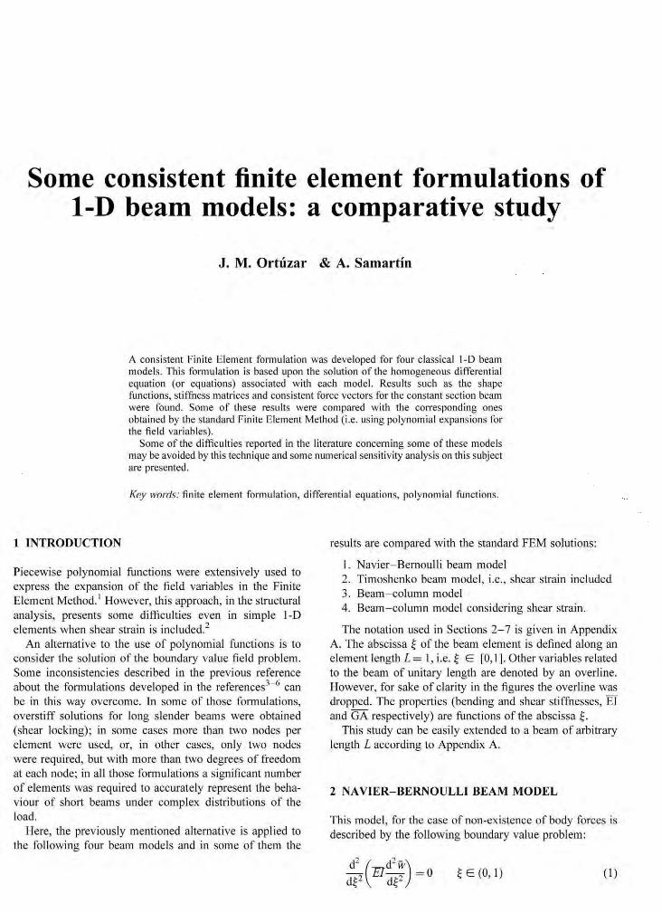
This model, for the case of non-existence of body forces is described by the following boundary value problem:

~E(O, l ) ( I)

la) External forces

'""'Trnrn-rrm q(x) -=--+='=.......-.-=-.......,,..-=,:----.-=-'=-=...-='--=--=--'=-'- n( x)

in(X)

(b) Deformed shape

~dx

(c) Section A : Internal forces

Fig. I. Navier- Bemoulli beam.

and the boundary conditions at ~; for i = 0,1

d w -d[=O;

(2)

where ~ 0 = 0 and ~ 1 = I , and w and 8 are the unknown deflection and slope at the abscissa ~ of the beam. w;, 0;, Q; and M; are data (see F ig. 1).

The solution of this problem is

(3)

where

(4)

T A = (A0 , At> A2 , A3)

f~ du f~ udu :F tCO= o (~ - u)El(u)' :!1(0= o(~-u)El(u)

The arbitrary constants A ; can be obta ined in terms of the essential boundary conditions, i.e.

(5)

where

(6)

0 0 0

0 0 0 Gd=

Uo- 11) (11 -lz)

0 Io it

and

fl d~ fo= oEJ(O' fl d~

1 - --1- o ~ EI(~)'

(7)

The deflections can be expressed in terms of the shape functions:

W(~) =t.mc;; 'd= Nw<Od (8)

where

~;rm = <Nt". rv2·. Nf, N:) (9)

~ 0 0 0

c- ~ -~ 0 ~ 0 0 - d - ~

-/1 - 12 I, -(~-[2) (I 0)

lo r, - fo Uo - I ,)

and [, I.

NJ"(O = 1 - -f.~F , + f.:J2 ( 11 )

The shape functions for the slope can be found from the previous functions:

- dw .,8 O(t) = - = /V" d c; d~ -- ( 12)

!! =(N/,Ni, /1/j,~)

Nf = d:; (i = 1, 2, 3, 4)

From the consideration of natural boundary conditions the arbitrary constants A; can be related to the boundary forces in the fol lowing way

where

and

0 0 0

0 0 - 1

0 0 0

0 0

0

- I

Then, the stiffness matrix is:

e.= G/J.d" '!i=Kd

with

fo

K=~ I,

- ~ -la

Uo- lJ)

J,

[2

- 1,

(J,- !2)

( 13)

(14)

(15)

(16)

- /o Uo - 1,)

-11 (!1- !2)

la -Cla-1,)

(1, - la) Ua- 2!, + !2)

(17)

If there were body forces applied in the beam, the right hand side of eqn ( 1) should be replaced with a tem1 con­taining these forces. The solution of the new boundary value problem permits to obtain tbe consistent equivalent forces.

The results for the case of the beam with constant section were obtained and they are summarised in Appendix B as a special case of the Timoshenko beam described in the fol­lowing section (fomlUiac (B. l . l ) to (8. 1.4)).

(a) External forces

I'TTTrrlrrrrrm q( X) --=~=-'-,...-=.:---.-'--='=-'"-.--=--=--='=-'=-",..---,o-=.._1 n( x)

m(x)

(b) Deformed shape r- et

eo _, _,-~ ~-H- -~ -~_;:;;--> -....:- -

WO ~

•w

3 T I MOSHENKO BEAM MODEL

The boundary value problem describing this model is

dw -~ E (0, 1) "j = d~ - f) G= E

2(1 + v)

and the boundary conditions at ~; for i = 0, I

-(dw -) -w= w; or CA df- fJ ; = Q;

8 = 0; or (El~~} =M;

(18)

(19)

where wand 8 are the unknown deflection and rotation of the normal section at the abscissa~ of the beam and A is the shear area. W;, 0;, Q. and M; are data and ~ 0 = 0 and ~ 1 = 1 (see Fig. 2). Note that the rotation (J is no longer the deri­vative of the deflection w.

Simi larly to the previous section, the shape functions, stiffness matrix, and consistent equi valent loads can be obtained. The results for the case of constant section are summarised in Appendix B (formulae (B.l. 1) to (8 .1.4)). It is interesting to point out that now, the shape function coefficients depend on the material properties g iven by the dimensionless coefficient J-1., where

(20)

w

Section A

MoOo QIMI t ~~I --!-- -+-- - -

0 - .. -

X - ·dx (c) Section A : Internal forces

Fig. 2. Timoshenko beam.

(a) E"1ernal forces

~''''' i " l ' J::r::n,,.,,,, , l,q(x) • • - • • • • - • • ,... - • • n(x)

l., .. .. ... ~.. ~ .. .. .. .. ' .. ~.. .. ' .. .. .. \ ' 1n(x)

(b) Deformed shape

X -dx (c) Section A : Internal torccs

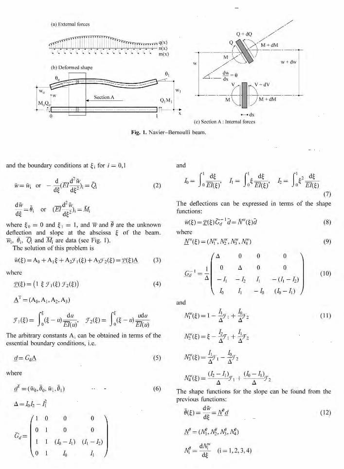
Fig. 3. Beam- column.

4 BEAM-COLUMN MODEL

It is assumed here that the axial forces of the beam-column are applied only at the beam ends. The boundary value problem is defined (see for example reference7

) by:

(21)

and the boundary conditions at ~; for i = 0, I

w= w; or - :~ ( £<~~) i - P( ~;) i = Q, (22)

~; = 0; or (El~~~); =M;

where P is the axial compressive force applied at both ends of the beam and w and 0 are the unknown deflection and slope at the absci ssa~ of the beam. w;, 0;, Q; and M; are data and ~ 0 = 0 and ~ 1 = 1 (see Fig. 3).

The shape functions, stiffness matrix, and equivalent force vectors for the case of constant section were obtained;

(a) External fur~es

rr:::r:r. r ']'. j .. l!:r::r 1" '1". : q(~ ) • • • • • • • • • • • • • • • • n(x )

• • • r:. • • '• • • • '· • • • • • '• m(x)

(b) De formed shape

they are presented in Appendix B as a special case of the general beam-column model with shear strain to be described later ((8.2.1) to (B.2.4)).

5 BEAM-COLUMN MODEL WITH SHEAR STRAJN

This model is a Timoshcnko beam in which axial forces arc applied at the beam ends similarly to the previous case. Then the problem is defined by the equations:

dd~ (GA-y - lfl) = o

where

dw -~ E (0, 1) 'Y = d~ - 0 C= E

2( I + v)

-dx

(~)Section A: lnlemal forces

(23)

Fig. 4. Beam- column with shear strain.

and the boundary condi tions at ~ i for i = 0,1

or CA(dw -e) -#). = Q-· d~ j I I

O=Oj or (El~:); =M;

(24)

where A is the shear area, Pis the axial compressive force applied at both ends of the beam, and w and e are the unknown deflection and rotation of the nonnal section at the abscissa~ of the beam. w;, 0;, Q and M; are data and ~ 0 = 0 and ~ 1 = I (see Fig. 4). In Appendix B the shape functions, stiffl1ess matrix and equivalent forces vector for the constant section situation are presented (formulae (B.2.1) to (B.2.4)).

It can be observed that in al l the previous models the shape functions satisfy the following well known properties in the limit i.e.:

I. Interpolation 2. Rig id body movements 3. Constant strain properties

6 FINITE ELEMENT APPROXIMATIONS

6.1 Introduction

An alternative to the earlier described approach is to trans­form tbe corresponding boundary value equations into weak fotms that are suitable for appljcation of the FEM. In this case the following results are reached:

Sti ffness matrix for Navier-Bernoulli and Timoshenko beam models:8

Ji = f~llT DBd~ (25a)

Stiffness matrix for beam- column model

(25b)

Stiffness matrix for beam- column model with shear strain

(25c)

Consistent force vector

(26)

where the matTices ll and J2 are dependent on the model under consideration and q and m are the distributed vettical forces and moments along the beam (see Fig. l).

ln the case of the Navier-Bemoulli beam and in the beam-column model, the expressions for matrices ll and

J2 can he written as follows:

B= (d2!:r) D=El - de - (27)

For the Timoshenko beam and the beam- colwnn model with shear strain the expressions for the earlier mentioned matrices become:

( ( dt) ) (El 0 )

I!~ ( d~ -ft') !2~ 0 CA (l&)

If the shape functions H. correspond to the ones obtained in the previous sections for the beam of constant section and are used in eqns (25) and (26), then the results forK and f~q are identical to those presented in Appendix B.

However these shape functions can be introduced in the fomlUla even for the cases of beams with variable section and the result obtained then represents a good approxi­mation of the exact solution, which in many cases cannot be analytically found.

In order to estimate the accuracy of this type of approxi­mation, the stiffness matrix of some constant section beam models wi ll be computed using eqns. (25) with shape func­tions corresponding to different and simpler beam models. Namely, two cases wi ll be analysed:

(a) Beam-column model using Hennitian polynomials as shape functions. (b) Beam-column model with shear strain using the shape functions of the Timoshenko beam model.

6.2 Beam-column model

The expression eqn (25a) for the stiffness matrix becomes now:

K = El f1

{ (d2!:r)T d2

!:r - c:lt~lN}dt - o de d~2 - - .,

=Ko-alKa (29)

where N" and!! are the shape functions vectors defined in (B.l.l), for the special case of the Navier Bernoull i model, and a is given by the following expression :

a= .r;, (30)

Ko represents the stiffness matrix of Navier- Bemoulli beam (B.1.2) (for the particu lar case of Navier Bernoulli model), and the expression for K.a is as follows:

36 3 -36 .., _)

.., 4

.., - I

f( =El _) - _)

_Q 30 -36 -3 36 -3 (3 1)

3 - 1 ..,

-_) 4

0.8

N 0.6

.-< 0.4

0.2

0.8

N 0.6

~· 0.4

0.2

(I

2

1.5

.,. ~·

0.5

()

IE- 0.5

IE- 0.5

1&-0.5

I E--D.S

Consistent solution

IEO.O

a

IEO.O

a

IEO.O

a

IEO.O

(J.

--------

IEO.S

IEO.S

IEO.S

IEO.S

Lincari7:cd solution

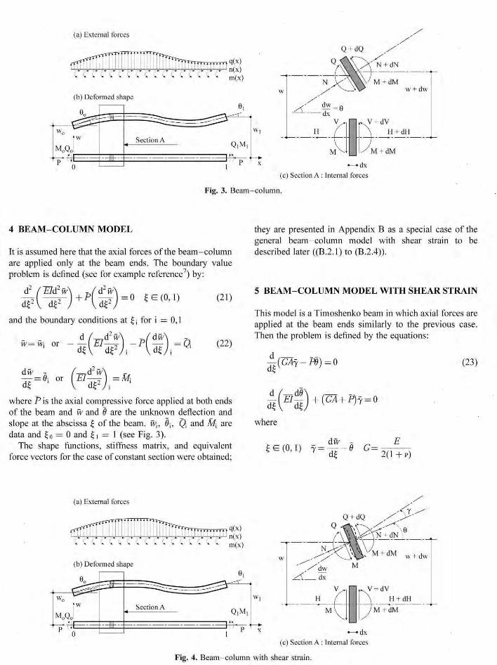
Fig. 5. Coefficients of the stiffness matrices of the beam co lumn in func.tion of the load.

lt is in teresting to compare the coefficients of th is approxi­mate stiffuess matrix with those of the 'exact ' or consistent one, derived in Section 4. This comparison will be carried out as a function of the dimensionless coefficient a. ln order to nonn alize the stitli1ess matrix coefficients for dif· ferent values or a they are divided by the corresponding ones for a = 0, i.e. the following quotients Aij are introduced:

ku(a) i<U A;i = --=I

k;j(O) kij (32)

with fS. = { kij}, and, k;j and k;j , which represent the

coefficients kij of the stiffness matrices of models 1 (Navier- Dernoull i beam) and 3 (Beam-column), respec­ti vely, which can be obtained as particular cases in the tables in Appendix B.

In Fig. 5, two sets of values of Aij are represented, in a semilogari thmic scale. The first one corresponds to the coef­ficients kij(a), given in (B.2.2) for the particular case of the beam column without shear strain, which can also be calcu­lated consistently using eqn (25) with the shape functions (8.2. 1) for that particular case, and the second one corre­sponds to those coefficients but calculated according to the approximate form ula eqn (29).

6.3 Beam- column model with shear strain

Similarly to the previous case, the stiffness matrix for a beam element becomes:

+ _!_ ( df!v -JI) T ( df!v _ t1) JJ- d~ - d~ -

- ci [ ( d~) T!! + ~ ( d~v) - fiT!!] } d~

=Ko-a?K.G (33)

with

(34)

where ~ and!/ are the shape function s vectors defined in (B .1.1 ), K.o corresponds here to the stiffness matrix of Timoshenko beam (B.I.2), and the Ko can be expressed as follows:

cl c2 - c l c2

KG=El cz c) - c2 '4

(35) -cl - C':l cl - c2

- c2 CJ

where

(36)

c,= - - - 72JJ-I ( l 2 ) - ~6 10

c3 = ~6 ( 2JJ- [ 1 - 12tt] + ~~~)

c4 =- ~~ (2tt[24JJ-+ 1] + 3'o)

~o = I+ 12tt. The coefficients of the stiffness matTix K obtained in (33) wi ll be next compared to their respective ones obtained in Section 5, in function of the dimensionless parameters a and IL· As in the beam column model without shear strain, it is interesting to introduce the following coefficients f...ij ,

where

kij(a, tt)

/<ft(O, JJ-) (37)

with K. = { kii }, and kij can be J0 or kij. These represent the coefficients kij of the sti ll'ness matrices or models 2

(Timoshenko beam) and 4 (Beam-column wi th shear strain), respectively.

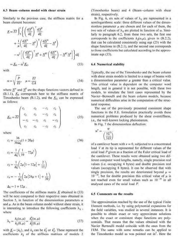
Jn Fig. 6, six sets of values of f...ij are represented in a semilogarithmic scale: three different values of the dimen­sionless parameter IL are chosen and tor each of them, the two sets of values of '-u are plotted in function of a. Simi­larly to paragraph 6.2, from these two sets, the first one corresponds to the coefficients kij(et,tt), given in (8.2.2), that can be calculated consistently using eqn (25) with the shape functions in (8.2.1), and the second one corresponds to those coefficients but calculated according to the approx­imate eqn (33).

6.4 Numerical stability

Typically, the use of the Timoshenko and the beam column with shear strain models is limited to a range of beams with a dimensionless parameter p, greater than a critical value. This critical value is dependent on the computer word length, and in general it is not possible, w ith these two models, to simulate the limit cases represented by the Navier-Bemoulli and the beam column models, because numerical difficulties arise in the computation of t11e struc­tural response.

The use of the previously presented consistent shape functions in the f.E. formulation practically avoids these numerical problems produced by the shear overstiffness, i.e., the well-known locking phenomenon.

In fig. 7 the dimensionlcss deflection:

* w w = ( VL

3)

3El

or a cantilever beam wi th v = 0, subjected to a concentrated load V at its tip is represented for different values of the axial load P given as a fraction of the Euler critical load of the cantilever. These results were obtained using two dif­ferent computer word lengths, namely, sing le precision reaJ values (i.e. occupying 4 bytes) and double precision real values (occupying 8 bytes). It can be observed that with single precision, the results are deteriorated beyond p, = 10- 10

, but for double precision this critical value of p, is not reached even tor small values such as I 0 -20 in all analysed cases of the axial load P.

6.5 Comments on the results

The approximation reached by the use of the typical Finite Element methods, i.e. by using polynomial expansions for the field variables, was studied in several instances. It is possible to obtain exact or very approximate solutions when the exact or consistent shape functions are poly­nomials. That means that the values obtained with the Navier Bemoulli model coincide wit11 the ones from the FEM. The same with some remarks can be applied to the Timoshenko model as was pointed out in2

. Here the

0.8

0.6

~ 0.4 -0.2 -

0 IE-0.5

2

1.5

"' ~

H.S -

0 IE-0.5

0.8

; : 0.6 -

0.4

0.2

l E- 0.5

2

1.5

..,. ~:

0.5

0 IE-0.5

Consistenl solution

Lincarized solution

for 1.1 e4ual to 0.00 1

IEO.O

a

IEO.O

a

IEO.O

a

!EO.O

a

--------

0.01

IEO.S

------------,,

IE0.5

IE0.5

----------------

0.1

\ \

\ \

\ \

' ' '

Fig. 6. Coefficients of the stiffuess matrices of the beam column with shear strain in function of the load.

results of the two last models are compared, namely beam­column and beam-column with shear strain.

In the case of the beam column, from Fig. 5 it can be observed that in general the stiffi1ess matrix obtained for the linearized solution is stiffer than the consistent one for values of IX greater than 10°'5• However, the linearized coefficient k11 has a negligible difference from the consistent one for the range of normal values of IX. The largest differences between coefficients of both sti ffness

matrices occur for coefficients k22 and k24 for large values of a.

Similarly, in Fig. 6, the coefficients of the consistent and linearized stiffness matrices of the beam column with shear strain are compared for three different shear strain levels. In general, for p. less than 0·00 l the comments given previously for the beam column without shear strain are valid. For very large values of the shear strain the di fferenccs between coefficients k11 moderately

16.E+OO ---1

14.E+OO

12.E+OO

::: 8.E+OO

6.11+00

2.E+OO

00."+0() l.OOE-()5

---11

I.OOE- 10

J.l

------Il l

I.OOE- 15

P=O

I.OOE- 20

Fig. 7. Cantilever beam of length L su~jccted to an axial load P and a lateral load V at its tip (material properties El and CA):

w• = ~ = ~· p. = -dJh = Z, N;,,. = ~ = ..l[i where w represents the vertica l deflection under the load at the tip.

\ID) \)m) In addition : 1: w* computed in double precision. 11 : w* computed in sing le precision. Il l: w* computed in double p1•ecis ion neglecting the

effect o f shear strain.

increase, but these differences become very large for k22

and k24•

7 CONCLUSIONS

The use of shape functions derived from the solutions of the homogeneous differential equations governing a given beam model in the FEM (these functions are not necessarily polynomials), leads to results that are much more accurate than those obtained with the standard polynomial ft.mctions of the FEM when one element is used.

The consistent formulation avoids some of the inconsis­tencies reported in the literature concerning the use of finite elements to model beams with shear strain.

The consistent shape functions determined may also be used to obtain the vectors and matrices of elements with longitudinal variation of the cross sections using the Finite Element technique. The results found in this way, although approximate, would be more accurate than those obtained with the standard polynomial shape functions.

However, the determination of the consistent shape func­tions demands an important programming and computing effort for each one of the different beam models considered, un like standard polynomial functi ons which are much more versatile.

APPENDIX A

The four consistent beam models considered were presented in the main text for a beam of unity length. The abscissa,~,

is equal to:

~ = ~ L

where xis the abscissa of the general beam of length L.

The other variables used in the beam of unitary length are denoted in the paper by an overline. They are equal to the corresponding variables of the general beam of length L, except for the following ones:

- El El= [2'

- M M=y· q = qL, n = nL

(AI)

where w, El, M, q and n are the deflection, llexural stiff­ness, end moment and distributed vertical and horizontal forces, respecti vely of the beam o f length L (E is Young's modulus and 1 is the moment of inertia) .

These expressions pem1it to transfom1 the expressions of the unitary length beam into a general form for a beam of length L.

APPENDIX B

In the following tables, the shape functions, stiffness matrices and consistent load vectors for two load cases rele­vant to the four consistent beam models are presented.

The shape functions correspond to a beam of unity length and satisfy the following equations:

(B 1.5)

and

om=!!Ii (B 1.6)

where

(B 1.7)

The extension of these results to the general beam of length L follow the same expressions as given in Appen­dix A.

Table 1. Timoshenko beam. The Navier Bernoulli beam formulae are found from the Timosbenko beam by assuming p. = 0 a nd Llo = 1.

Timoslleuko beam

Shape functions

Deflection w sllape functions

Nlw(~) = _!_(( I + I21J.) - I 21J.~-3~2 +2~3) ~0

N,w(~} = _!_((I +6j.J.}~ - (2 +6j.J.}~~+~3} - ~0

N3w(~} = _!_(l2j.J.~ + W-2~3) ~0

Nt (~) = _!_(( -6J.l)~ +(6J.1 - I )~2 +~3) ~0

Rolation '9" sllapc functions

N 18(~) = _!_( -6~ +6~2) ~0

a I 2 N, (~) = -((l • I 2 J.1) -2(2 +61J.)~ •3~) - ~0

N36(~ = _!_(6~- 6~2) ~0

N46(~l = _!_(2(61J. - 1 >~ • 3e) ~0

Stiffness malrix

[ 12

6 - 12 6

El 6 4(1 +3 j.J.) -6 2(1 -6 J.l ) K= -

~(l - 1 ~ -6 12 -6

2( l - 6J.1) - 6 4(1 +3J.l)

Consistent force vectors

Distributed vertical force q

q ( -( +) ; -( 112) ; - ( +) ; ( 112 ) )

Distributed moment m -~ (I ; - 6J.l; - I Ao

: - 6 J.l )

Stiffness matrices and load vectors correspond also to a beam of unity length. They satisfy the equation:

e=Kd (8 1.8)

Vector p is an end load vector (see Fig. 1). The consistent load vectors presented in this appendix are a function of a distributed load or moment.

The following notation was used in the Table 1 and Table 2: E is Young's modulus and, T the moment of inertia.

For the Timoshenko beam model, specific notation was used:

Fl El .10 =I + 1 2~-t ~-t = CA = GAL2 (82.5)

[B.l .l .a]

[B.l.l.b)

[B.l.2]

[B.l.J]

(lU.4]

where G is the shear modulus and A the shear area. For the ordinary Navier Bemoulli beam J.t = 0 and .10 = 1.

For the beam- colwllll model the following notation is applied:

a= a=r:f c =cosa

s=sin a .11 =2(1 -c)-sa (82.6)

where P= Pis the applied axial load, and if shear strain is included then the new variables are introduced:

0! = aJI + a 2p. c = cos 0! S= sin 0!

.12 = 2(1 -c)( I + a 1 J.t)- SO! ( 82.7)

Table 2. Beam-column with shear strain. The beam-column without shear strain expressions are found by assuming p. = 0.

Bcaru column with shear strain

Shape function.~

Deflection w shape functions

Nt<~> = ~ Cl(I •a\1)(J -c) -siX] ·s~ • 1(1 •a"J.t)O -c)Jcos(iX~Hs( l •a211)Jsin(a~)l 2 -

N,w(~) = _a_(( ea -s( 1 •a211)J •< 1 -c)iX~ -(ea - se 1 +a111)Jcos(iX~) • 1(1 - c)( I •a"11)-siXJsin(iX~))

- a~Ll.2

w 1 ') - -- ., - - - , -N3 (~) = -(((l +a·J.l)( l - c)] - s ~ - ((1 +a·ll-)(1 -c) ]cos(a~) -+(s( l +a·l!)]sin(a~))

~ -N4w(~) = ~((s(l •a211) -iXH 1 -c)~ - (s(l +a2~t) -a]cos(a~) - ((1• a2~t)O -c))sin(a~))

a-.0.2

[B.2.l.a]

Rotation l1 shape functions

2 N 16(~) = ~(s(l ... a2J.t)- ((l +a2!!)0 -c))sin(iX~)-Is( l •a2~t)]cos(~))

a.0.2

N,6(~) = ...!...c<r - c)( I •a211) +tciX-s(l •a~11) Jsin(iX~)+I(l -c)(l •a211)-sa)cos(a~)) - .0.2

2 N36(~) = ~ ( -s( l +a2~t)• ((I • a2J.l){l -c)]sin(~) •Is( I •a2J.l))cos(~))

a.0.2

N46m = -k<<I-c)(l •a2

11)-tiX-s(I •a211)Jsin(iX~H(l-c)(l +a211) ]cos(~))

(B.2.l.b]

Stiff uess matrix

-- (I+ a 2J.l)( l -c) --(I • a2

11)( 1 - c) as - as

(I •a211)(1-c) ~(so • a211l -ea) - (1 •a211)(1-c)

a -- .,

- a~ 0

-;(a - s(l +a"jt)) a· a·

K =El- -- -- [B.2.2] .0." -as -(I •a211){1 - c) as - (1 •a: ll)(J -C)

- -( I •a=11)(1-c) a. - - ., - (1 •a=11)( I - c) a - • --- (a - s(l•a-11)) ~(s(l +a"ll) - c a)

a2 a·

Consistent force vectors

Di~tributed vertical force q Distributed moment iii

-a2~ [ ··-~(1 :'' - ((%2(1 +c) • 2.0.2- 2s a( I +a 21!)( -_q_ m (I -c)a · ll -- [B.2.4] 2a2.0.: - a=.o.2 .0.2 2(1 -c) -sa

1(%20 .. c) . 2~ -2sa(I •a 2J.t>l (l -c)a211

fB.2.31

where a and Jl have already been defined. It is found that for the case of the beam column without shear strain:

2. Friedman, Z. and Kosmatka, J . B., An improved two-node Timoshenko beam finite element. Computers and Slruclures, 1993, 47(3), 473- 481.

(82.8)

REFERENCES

I. Turner, M. J., C lough, R. W., Martin, H. and Topp, L. J., Stiffness and deflection analys is of complex structures. ]. Aeron. Sci., 1956, 23, 805-823.

3. Nicke ll, R. E . and Secor, G. A., Convergence of consistently derived Timoshenko beam finite elements. lnt. }. Numer. Meth. Engng., 1972, 5, 243-253.

4. T homas, D. L., Wilson, J. M. and Wilson, R. R., Timoshenko beam finite e lements. j. Sound Vibr. , 1973, 31, 315-330.

5. Hughes, T. R. J., Taylor, R. L. and Kanoknukulchoii, W., A s imple and efficient plate e lement for bending. lnt. }. Numer. Meth. tngng .. 1977, 11, 1529- 1943.

6. Tessler, A. and Dong, S. B., On a hierarchy of confonning Timoshenko beam elements. Cam put. Stmct., J 98 1, 14, 335-344.

7. Samartln, A., Teoria e lemental de la viga-columna con apli­cacion al estudio de la estabilidad elastica de estructuras.

Publicacion AE-84-4, E.T.S. I.C.C.P. de Santander, Universi­dad de Santander, 1984.

8. Zienckiewicz, 0. C. and Taylor, R. L., The Finite Element Method, 4th edn. McGraw-H ill, New York, 1991.