SOME COMMENTS ON DESIGN-BASEDLINE-INTERSECT SAMPLING

WITH SEGMENTED TRANSECTS

LUCIO BARABESIUNIVERSITÀ DI SIENA

1

LINE-INTERSECT SAMPLING

• is a method for sampling units scattered over aLine-intersect samplingplanar region.

• In its , a unit is if a given line-segment (thebasic version sampled“ ”) intersects the unit.transect

• In forestry, line-intersect sampling has found widespread application forthe purpose of estimating and .plant abundance vegetative coverage

• Much recent attention has focused on line-intersect sampling for theassessment of for monitoring biodiversity ofcoarse woody debrisecosystems.

2

DESIGN-BASED LINE-INTERSECT SAMPLING

• Let be a of (given by T ßá ßT R" R fixed population units connectedcompact sets) scattered over the study region .V

• If represents a of , in the C T4 4fixed measurable attribute design-basedapproach population total the target parameter is usually given by the

7 œ C4œ"

R

4

• The design-based approach is convenient for line-intersect applicationsin order to avoid on unit shape and placementunrealistic assumptionsunder the .model-based approach

• Moreover, field researchers really wish to do not identify the modelparameters make predictions random total and of a , but they seek toestimate a .fixed population total

3

UNIT SELECTION

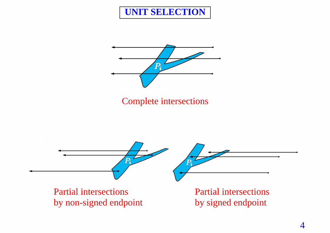
• The intersection of a unit is when the intersects thecomplete transectunit boundary as the containing the transect. Inas many times linecontrary, an intersection is .partial

• A unit is always if the intersection is complete.selected

• Partial intersections are usually handled by assuming that a transectendpoint is . In this case, units are by partial intersectionssigned sampledof the .signed endpoint

• In some designs units may be sampled by partial intersections of bothtransect endpoints.

4

UNIT SELECTION

Complete intersections

Partial intersections Partial intersections by non-signed endpoint by signed endpoint

5

DESIGN IMPLEMENTATION

• A transect of is identified by a on and a fixed length positionP ? Vdirection on .) 1Ò!ß # Ò

• The is practically implemented by selecting and .design ? )

• For each , an for each , the unit is) inclusion region is defined T4 i.e.sampled if is in the inclusion region? .

6

INCLUSION REGION

• The following figure shows the of a unit by assuminginclusion regionthat is the . In the ? transect midpoint yellow-colored complete setsintersections orange-colored partial intersections occur, while in the sets occur. The unit in the inclusion region.is

7

INCLUSION REGION

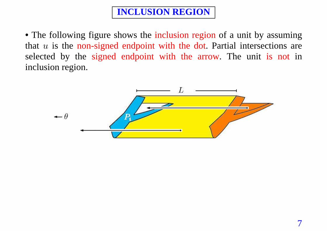
• The following figure shows the of a unit by assuminginclusion regionthat is the . Partial intersections are? non-signed endpoint with the dotselected by the . The unit insigned endpoint with the arrow is notinclusion region.

8

CONDITIONAL AND UNCONDITIONAL APPROACHES

• The “ ” is achieved by fixing and obtaining asconditional approach ) ?the realization of a suitable random variable .Y

• The “ ” is considered if and are realizationsunconditional approach ? )of two suitable random variables and .Y K

• Let us assume that D Ð?ß Ñ4 ) is a function outside the inclusionvanishingregion and exclusively on the depending transect position.

• The function D Ð?ß Ñ T4 4) represents a on the unit measurable quantityaccording to its with the intersection transect (for example the oflength the intersection).

9

KAISER'S ESTIMATORS

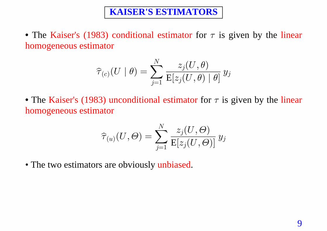
• The for is given by the Kaiser's (1983) conditional estimator linear7homogeneous estimator

7 ))

) )s ÐY ± Ñ œ C

D ÐY ß Ñ

ÒD ÐY ß Ñ ± ÓÐ-Ñ

4œ"

R4

44E

• The for is given by the Kaiser's (1983) unconditional estimator linear7homogeneous estimator

7 KK

Ks ÐY ß Ñ œ C

D ÐY ß Ñ

ÒD ÐY ß ÑÓÐ?Ñ

4œ"

R4

44E

• The two estimators are obviously .unbiased

10

AN EXAMPLE

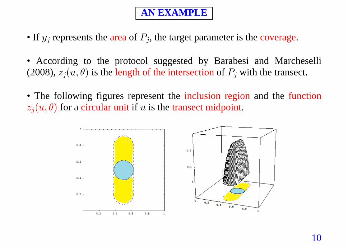
• If represents the of , the target parameter is the .C T4 4area coverage

• According to the protocol suggested by Barabesi and Marcheselli(2008), is the of with the transect.D Ð?ß Ñ T4 4) length of the intersection

• The following figures represent the and the inclusion region functionD Ð?ß Ñ4 ) for a if is the .circular unit transect midpoint?

11

AN EXAMPLE (continues)

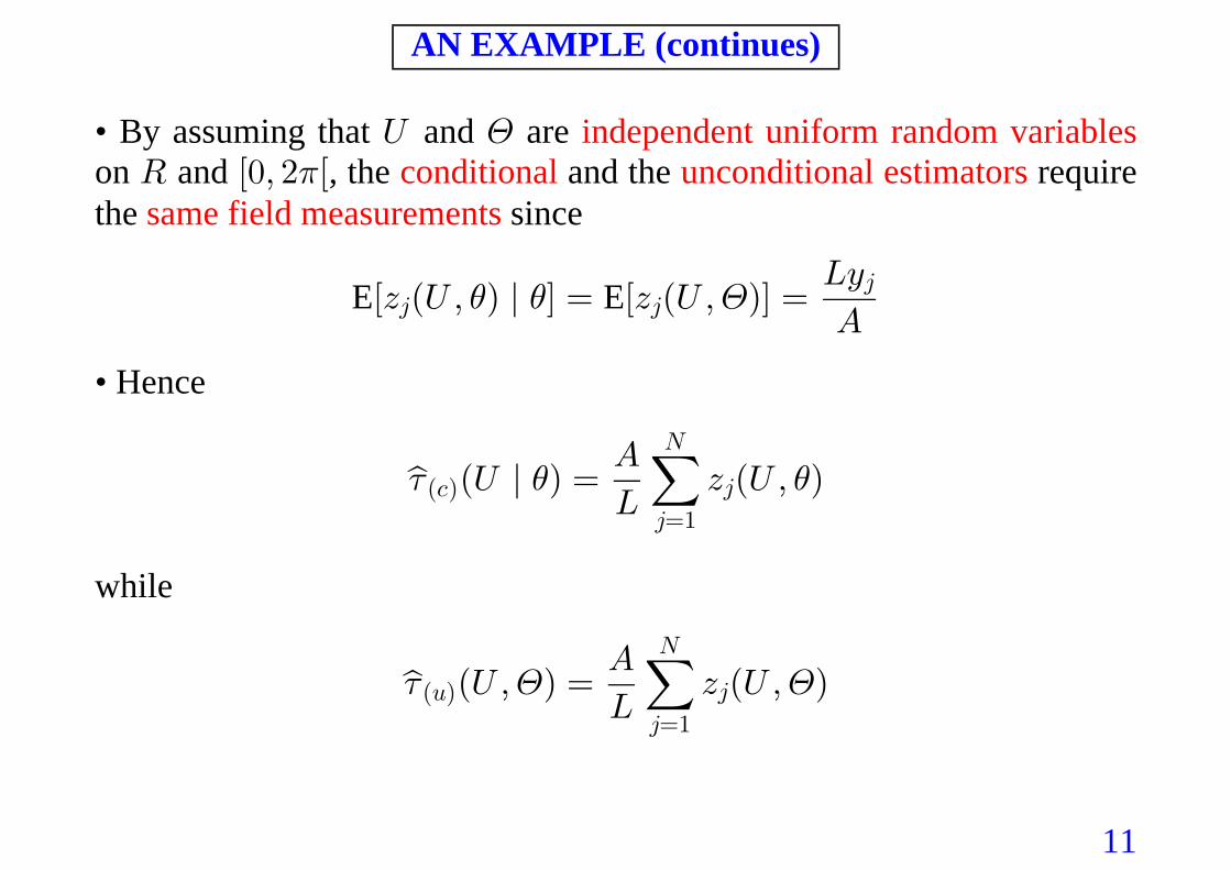
• By assuming that Y and are K independent uniform random variableson and V Ò!ß # Ò1 , the and the requireconditional unconditional estimatorsthe sincesame field measurements

E EÒD ÐY ß Ñ ± Ó œ ÒD ÐY ß ÑÓ œPC

E4 4

4) ) K

• Hence

7 ) )s ÐY ± Ñ œ D ÐY ß ÑE

PÐ-Ñ

4œ"

R

4

while

7 K Ks ÐY ß Ñ œ D ÐY ß ÑE

PÐ?Ñ

4œ"

R

4

12

DESIGN-BASED LINE-INTERSECT SAMPLINGWITH SEGMENTED TRANSECTS

• A is a fixed set of of totalsegmented transect oriented line segmentsOlength . A segmented transect .P may not be connected

• Segmented transects include (such as L-shaped or Y- radial transectsshaped transects) and (such as triangular or squaredpolygonal transectstransects), which are adopted in many national forest inventories.

• The Forest Inventory and Analysis (FIA) program of the U.S.D.A.Forest Service assumes a consisting ofnon-connected segmented transecta symmetric arrangement of .four Y-shaped transects

• Field scientists adopt this sampling protocol on the basis of the falsebelief anisotropy that segmented transect may capture in the population.

13

UNIT SELECTION AND DESIGN IMPLEMENTATION

• A population unit is if it is by a line segment ofsampled selected at leastthe transect.

• A transect is by a and a . segmented identified position direction? )

• As an example, may be characterized by the position radial transects ?of their and by the direction of the common vertex leading line)segment.

• The design is implemented by and .selecting ? )

• The turns out to be the of the inclusion regionsinclusion region unioncorresponding to each line segment of the transect (which may ).overlap

14

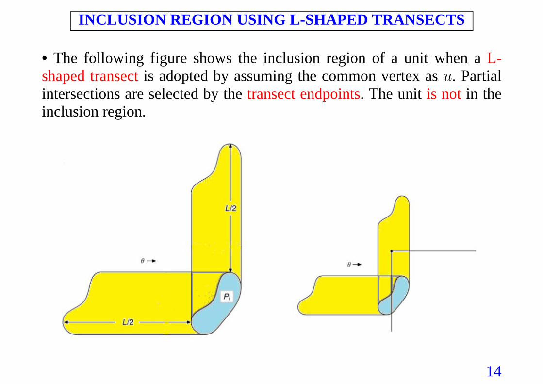
INCLUSION REGION USING L-SHAPED TRANSECTS

• The following figure shows the inclusion region of a unit when a L-shaped transect is adopted by assuming the common vertex as . Partial?intersections are selected by the . The unit in thetransect endpoints is notinclusion region.

15

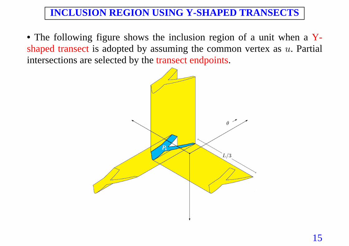
INCLUSION REGION USING Y-SHAPED TRANSECTS

• The following figure shows the inclusion region of a unit when a Y-shaped transect is adopted by assuming the common vertex as . Partial?intersections are selected by the .transect endpoints

16

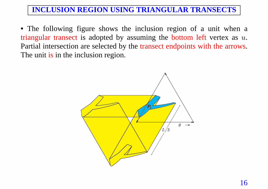
INCLUSION REGION USING TRIANGULAR TRANSECTS

• The following figure shows the inclusion region of a unit when atriangular transect bottom left is adopted by assuming the vertex as .?Partial intersection are selected by the .transect endpoints with the arrowsThe unit is in the inclusion region.

17

FIA-PROGRAM TRANSECTS

18

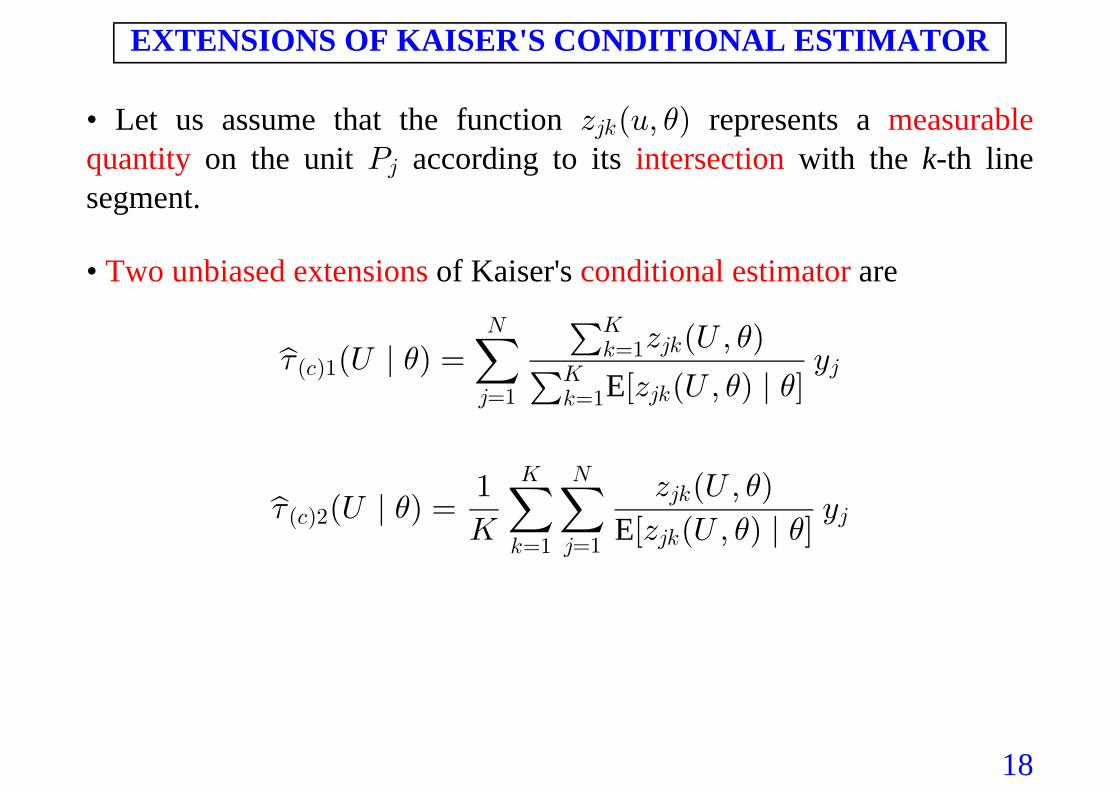
EXTENSIONS OF KAISER'S CONDITIONAL ESTIMATOR

• Let us assume that the function D Ð?ß Ñ45 ) represents a measurablequantity intersection on the unit according to its with the T4 k-th linesegment.

• of Kaiser's areTwo unbiased extensions conditional estimator

7 ))

) )s ÐY ± Ñ œ C

D ÐY ß Ñ

ÒD ÐY ß Ñ ± ÓÐ-Ñ"

4œ"

R5œ"O

45

5œ"O

454

E

7 ))

) )s ÐY ± Ñ œ C

"

O ÒD ÐY ß Ñ ± Ó

D ÐY ß ÑÐ-Ñ#

5œ"

O R

4œ"

45

454E

19

EXTENSIONS OF KAISER'S UNCONDITIONAL ESTIMATOR

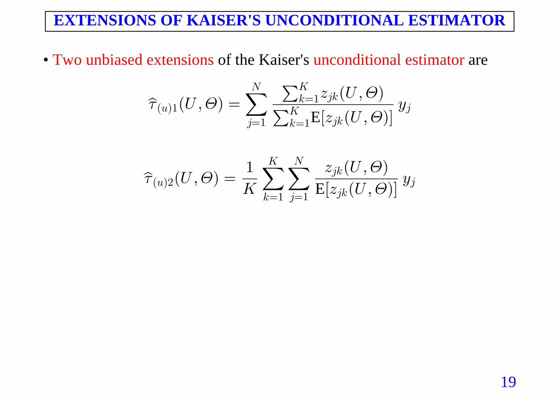
• Two unbiased extensions unconditional estimator of the Kaiser's are

7 KK

Ks ÐY ß Ñ œ C

D ÐY ß Ñ

ÒD ÐY ß ÑÓÐ?Ñ"

4œ"

R5œ"O

45

5œ"O

454

E

7 KK

Ks ÐY ß Ñ œ C

"

O ÒD ÐY ß ÑÓ

D ÐY ß ÑÐ?Ñ#

5œ"

O R

4œ"

45

454E

20

EXTENSIONS OF KAISER'S ESTIMATORS

• The ( and ) include the estimatorsfirst-type extensions i.e. 7 7s sÐ-Ñ" Ð?Ñ"

proposed by Affleck (2005).et al.

• The Forest Inventory and Analysis of the U.S.D.A. Forest Serviceutilizes estimators which are special cases of the second-type extensions( and ).i.e. 7 7s sÐ-Ñ# Ð?Ñ#

• The two conditional estimators if does notcoincide EÒD ÐY ß Ñ ± Ó45 ) )depend on for each , as well as the two unconditional estimators5 4coincide when does not depend on for each . This featureEÒD ÐY ß ÑÓ 5 445 Kis to most of the estimators usually adopted in the practice ofcommonsegmented-transect sampling.

• For it may even occur that some important protocols EÒD ÐY ß Ñ ± Ó œ45 ) )EÒD ÐY ß ÑÓ 5 445 K and this quantity does not depend on for each and hencethe four estimators are from the sampling effort perspective.equivalent

21

THREE IMPORTANT ISSUES

• While boundary effects straight- may be easily managed in the case of line transects serious more complex transect shapes, the problem is with .

• for a may be expressed since theNo preference particular estimatorvariances unknown population frame of the estimators depend on the .The conditional estimator )s (as well as the unconditional estimatorsrequire the since they involve the same fieldsame sample effortmeasurements. The could be preferred to theconditional approachunconditional approach measurement (or ) on the basis of vice versacomplexity.

• for a may be asserted since theNo superiority particular transect shapevariances of estimators based on different transect types (of the same totallength) depend on the . unknown population frame Straight-line transectsshould be since their field implementation is easier and edgepreferredeffects are easily handled.

22

AN EXAMPLE

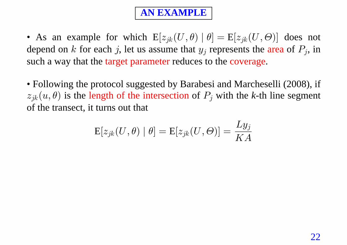
• As an example for which does notE EÒD ÐY ß Ñ ± Ó œ ÒD ÐY ß ÑÓ45 45) ) Kdepend on for each , let us assume that represents the of , in5 4 C T4 4areasuch a way that the reduces to the .target parameter coverage

• Following the protocol suggested by Barabesi and Marcheselli (2008), ifD Ð?ß Ñ T45 4) is the of with the -th line segmentlength of the intersection kof the transect, it turns out that

E EÒD ÐY ß Ñ ± Ó œ ÒD ÐY ß ÑÓ œPC

OE45 45

4) ) K

23

AN EXAMPLE (continues)

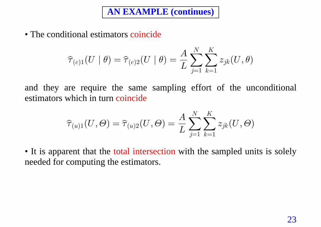
• The conditional estimators coincide

7 ) 7 ) )s sÐY ± Ñ œ ÐY ± Ñ œ D ÐY ß ÑE

PÐ-Ñ" Ð-Ñ#

4œ"

R O

5œ"

45

and they are require the same sampling effort of the unconditionalestimators which in turn coincide

7 K 7 K Ks sÐY ß Ñ œ ÐY ß Ñ œ D ÐY ß ÑE

PÐ?Ñ" Ð?Ñ#

4œ"

R O

5œ"

45

• It is apparent that the with the sampled units is solelytotal intersectionneeded for computing the estimators.

24

REPLICATED TRANSECTS

• As is usual in environmental protocols, 8 of the line-replicationsintersect design are usually performed. The goal is the selection of anappropriate strategy replicates for the placement of the .8

• By assuming the , the target parameter may beconditional approach 7expressed as an integral

7 œ"

E(V

7 )s Ð? ± Ñ ?Ð-Ñ6 d

• Accordingly, the estimation reduces to a Monte Carlo integration.

25

SIMPLE RANDOM SAMPLING OF REPLICATES

• The (equivalent to the )random sampling crude Monte Carlo integrationis achieved by generating independent transect locations 8 Y ßá ßY" 8

uniformly distributed on .V

• Two may be obtainedoverall estimators

7 7 ) )– – , Ð-Ñ6 Ð-Ñ6 " 8 3

3œ"

8

œ ÐY ßá ßY ± Ñ œ ± Ñ 6 œ "ß #"

87s ÐYÐ-Ñ6

• The estimators are , while –unbiased VarÒ7 Ð-Ñ6Ó œ SÐ8 Ñ" .

• The arevariance estimators

Vars Ò ÐYs7 7 7– – , Ð-Ñ6 Ð-Ñ6

3œ"

8

3#Ó œ Ð ± Ñ Ñ 6 œ "ß #

"

8Ð8 "ÑÐ-Ñ6 )

• It is easily proven that as .– –Vars Ò7 7Ð-Ñ6 Ð-Ñ6"Î# .Ó Ð Ñ Ä Ð!ß "Ñ 8 Ä ∞7 a

26

NON-ALIGNED SYSTEMATIC SAMPLING OF REPLICATES

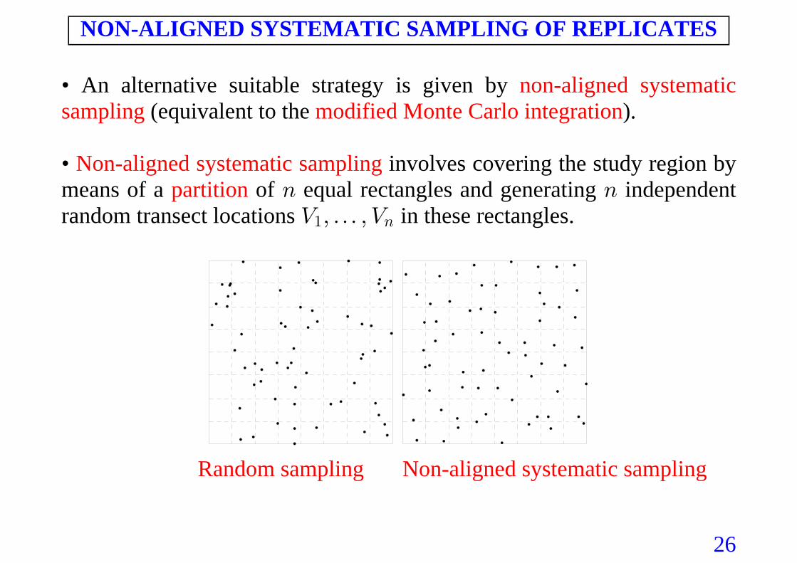
• An alternative suitable strategy is given by non-aligned systematicsampling ( .equivalent to the )modified Monte Carlo integration

• Non-aligned systematic sampling involves covering the study region bymeans of a of equal rectangles and generating independentpartition 8 8random transect locations in these rectangles.Z ßá ß Z" 8

Random sampling Non-aligned systematic sampling

27

NON-ALIGNED SYSTEMATIC SAMPLING OF REPLICATES

• The strategy provides the two overall estimators

7 7 ) )– – , Ð-Ñ6 Ð-Ñ6‡ ‡

" 8 3

3œ"

8

œ ÐZ ßá ß Z ± Ñ œ ± Ñ 6 œ "ß #"

87s ÐZÐ-Ñ6

• The estimators are .unbiased

• Moreover, , – –Var VarÒ Ò7 7Ð-Ñ6‡

Ð-Ñ6Ó Ÿ Ó i.e. non-aligned systematic samplingis always to preferable simple random sampling.

28

NON-ALIGNED SYSTEMATIC SAMPLING OF REPLICATES

• The estimators are .7– Ð-Ñ6‡ very efficient

• Barabesi and Marcheselli (2003) show that if VarÒ s7 7–Ð-Ñ6‡ Ó œ SÐ8 Ñ#

Ð-Ñ6

is a Lipschitz function.

• Barabesi and Pisani (2004) show that if VarÒ s7 7–Ð-Ñ6‡ Ó œ SÐ8 Ñ$Î#

Ð-Ñ6 is anelementary function.

• Barabesi and Marcheselli (2008) show that withVarÒ7–Ð-Ñ6‡ Ó œ SÐ8 Ñα

" Ÿ Ÿ $Î#α if 7sÐ-Ñ6 is a function and withpiecewise Sobolev$Î# Ÿ Ÿ #α if 7sÐ-Ñ6 is a function.Sobolev

29

NON-ALIGNED SYSTEMATIC SAMPLING OF REPLICATES

• I is a Lipschitz functionf , a for 7 7s ÒÐ-Ñ6 consistent estimator Var – isÐ-Ñ6‡ Ó

Vars Ò ÐZs7 7 7– – – , Ð-Ñ6‡ #

#3œ"

8

3 Ð-Ñ63 Ð-Ñ6Ó œ Ð ± Ñ Ñ 6 œ "ß #%

&8Ð-Ñ6 ) 7

where is the average of the quantities –7 )Ð-Ñ63 7s ÐZ ± Ñ 4Ð-Ñ6 4 over the indexes corresponding to the rectangles adjacent to the -th rectangle.i

• Moreover, as – –Vars Ò s7 7 7Ð-Ñ6 Ð-Ñ6‡ "Î# ‡ .

Ó Ð Ñ Ä Ð!ß "Ñ 8 Ä ∞7 a if Ð-Ñ6 is aLipschitz function.

• The turns out to be for less regularvariance estimator conservativefunctions and the previous pivotal quantity produces large-sampleconservative confidence intervals even if is an elementary function7sÐ-Ñ6

or a Sobolev function.

30

FINAL REMARKS

• Barabesi and Marcheselli (2005, 2008) have proven that a furtherstrategy, i.e. locally antithetic non-aligned systematic sampling, may bemore effective than non-aligned systematic sampling. However, locallyantithetic non-aligned systematic sampling may be more involved in thefield.

• The efficiency of under non-aligned systematic sampling theunconditional approach worse conditional approach is than under the .This problem occurs since integrals of 3-dimensional functions must beevaluated in this case and the “ ” takes places withcurse of dimensionalityrespect to the unconditional approach. This drawback may motivate thepreference conditional approach of the over the unconditional approachwhen the sampling effort for collecting field measurements is the same.

31

REFERENCES

Affleck, D.L.R., Gregoire, T.G. and Valentine, H.T. (2005) Design unbiasedestimation in line intersect sampling using segmented transects, Environmentaland Ecological Statistics , 139-154.12

Barabesi, L. (2007) Some comments on design-based line-intersect sampling byusing segmented transects, Environmental and Ecological Statistics 14, 483–494.

Barabesi, L. and Marcheselli, M. (2003) A modified Monte Carlo integration,International Mathematical Journal , 555-565.3

Barabesi, L. and Marcheselli, M. (2005) Some large-sample results on amodified Monte Carlo integration method, Journal of Statistical Planning andInference , 420-432.135

Barabesi, L. and Marcheselli, M. (2008) Improved strategies for coverageestimation by using replicated line-intercept sampling, Environmental andEcological Statistics .15

Barabesi, L. and Pisani, C. (2004) Steady-state ranked set sampling forreplicated environmental sampling designs, .Environmetrics 15, 45-56

Kaiser, L. (1983) Unbiased estimation in line-intercept sampling, Biometrics 39,965-976.

32

SPAZI DI SOBOLEV

• Lo spazio di Sobolev , dove , contiene funzioni[ Ð Ñ : − Ò"ß∞Ñ"ß: ‘0 − P Ð Ñ 1 − P Ð Ñ: :‘ ‘ per cui esiste una funzione (la cosiddetta derivatadebole di ordine ) per la quale:

( (‘ ‘

0ÐBÑ .B œ .B: :wÐBÑ 1ÐBÑ ÐBÑ

per ogni funzione test .: ‘− G Ð Ñ"

• Equivalentemente, se e solo se è 0 − [ Ð Ñ 0"ß: ‘ quasi ovunquedifferenziabile in modo che per ogni si ha0 − P Ð Ñ Bß C −w : ‘ ‘

0ÐBÑ œ .>0ÐCÑ 0 Ð>Ñ(C

Bw

33

SPAZI DI SOBOLEV

• Lo spazio di Sobolev [ Ð Ñ"ß" ‘ coincide con lo spazio delle funzioniassolutamente continue e quindi può contenere funzioni molto irregolari.Una funzione di Lipschitz è equivalente ad una funzione in [ Ð Ñ"ß∞ ‘ .

• Una estensione di [ Ð Ñ [ Ð Ñ"ß: =ß:‘ ‘ è data dallo spazio di Sobolev dove è un intero.=   #

• Lo spazio è definito in modo ricorsivo, ovvero i membri di[ Ð Ñ=ß: ‘[ Ð Ñ 0ß 0 − [ Ð Ñ [ Ð Ñ#ß: w "ß: $ß:‘ ‘ ‘ sono tali che , i membri di sono taliche , e così via.0 ß 0 ß 0 − [ Ð Ñw ww #ß: ‘

34

SPAZI DI SOBOLEV

• Supponiamo un insieme centrato in la cui frontiera soddisfaÐ ß Ñ- -" #

l'equazione

± ? ± ± ? ± œ" " # #; ; ;- - 3

con e . ; − Ò"ß∞Ñ !3 La lunghezza dell'intersezione fra un transetto in? e l'insieme è data da

-Ð?Ñ œ #Ð ± ? ± Ñ Ð?Ñ3 -; ; "Î;" Ò ß ÓI - 3 - 3" "

• Evidentemente e- − [ Ð Ñ ? œ"ß: ‘ , dal momento che nei punti - 3"

? œ - 3" la funzione non è differenziabile, ma ammette solamente unaderivata debole di opportuno ordine . Questa semplice funzione soddisfa:la condizione di solo per .Lipschitz ; œ "

35

SPAZI DI SOBOLEV

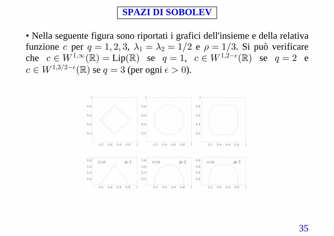
• Nella seguente figura sono riportati i grafici dell'insieme e della relativafunzione per , e . Si può verificare- ; œ "ß #ß $ œ œ "Î# œ "Î$- - 3" #

che Lip se , se e- − [ œ ; œ " - − [ ; œ #"ß∞ "ß#Ð Ñ Ð Ñ Ð Ñ‘ ‘ ‘%

- − [ ; œ $ !"ß$Î#%Ð Ñ‘ se (per ogni ).%

0.2 0.4 0.6 0.8 1

0.2

0.4

0.6

0.8 q=1cHuL

0.2 0.4 0.6 0.8 1

0.2

0.4

0.6

0.8

1

0.2 0.4 0.6 0.8 1

0.2

0.4

0.6

0.8 q=2cHuL

0.2 0.4 0.6 0.8 1

0.2

0.4

0.6

0.8

1

0.2 0.4 0.6 0.8 1

0.2

0.4

0.6

0.8 q=3cHuL

0.2 0.4 0.6 0.8 1

0.2

0.4

0.6

0.8

1

36

SPAZI DI SOBOLEV

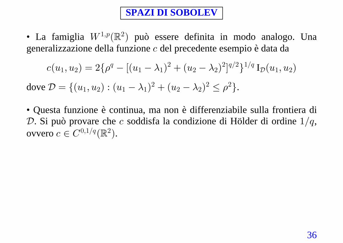
• La famiglia [ Ð"ß: ‘#Ñ può essere definita in modo analogo. Unageneralizzazione della funzione del precedente esempio è data da-

-Ð? ß ? Ñ œ #Ö ÒÐ? Ñ Ð? Ñ Ó × Ð? ß ? Ñ" # " " # # " #; # # ;Î# "Î;3 - - IW

dove W œ ÖÐ Ñ À? ß ? Ð? Ñ Ð? Ñ Ÿ ×" # " " # ## # #- - 3 .

• Questa funzione è continua, ma non è differenziabile sulla frontiera diW. Si può provare che - "Î; soddisfa la condizione di Hölder di ordine ,ovvero .- − G Ð Ñ!ß"Î; ‘#

37

SPAZI DI SOBOLEV

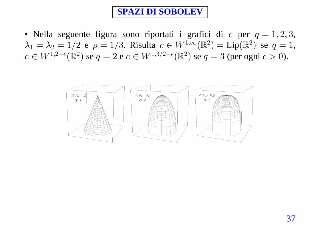
• Nella seguente figura sono riportati i grafici di per ,- ; œ "ß #ß $- - 3" #

"ß∞œ œ "Î# œ "Î$ - − [ œ ; œ " e . Risulta Lip se ,Ð Ñ Ð Ñ‘ ‘# #

- − [ ; œ # - − [ ; œ $ !"ß# "ß$Î#% %Ð Ñ Ð Ñ‘ ‘# # se e se (per ogni ).%

cHu1, u2Lq=1

cHu1, u2Lq=2

cHu1, u2Lq=3