some aspects of time-dependent
TRANSCRIPT

J
SOME ASPECTS OF TIME-DEPENDENT . r I'
ONE-DIMENSIONAL R&~DOM WALKS
by
Thesis submitted to the Graduate Faculty of the
Virginia Polytechnic Institute
in partial fulfillment for the degree of
DOCTOR OF PHILOSOPHY
in
Statistics
__ ~. ~ ~ __ 'J.~ ~:......::::..: --!-d =---_
Dr. C. E. Hall
Mr. Brian W. Conolly
September, 1968
Blacksburg, Virginia

.,
... "-,,,' .. "11.,"\.; .... ,...... I
LIJ ¢G:,S5 V8S6 .1968 GS C!.2.

TABLE OF CONTENTS
CHAPTER PAGE
I. INTRODUCTION 1
II. MATHEMATICAL REQUIS ITES •...••••.•••••.••.•..•••.• 8
2.1 Introduction •.•••••••.•••.•••••••••.•.•••..• 8
2.2 The-Laplace Transformation ..••.••••••.•.••.• 8
2.3 Modified Bessel Functions and Their Properties .....•••••.••••••..••..••••.••.••. 16
2.4 The J-function •..•••••..•••...•.••••••..••.• 19
2.5 The Generalized Hypergeometric Function .•..• 24
2.6 Stable Distributions ••..•....•....•••. ~ •••.. 25
III. FIRST-PASSAGE TIMES AND MAXIMA FOR THE RANDOM WALK WITH NEGATIVE EXPONENTIALLY DISTRIBUTED INTERVALS BETWEEN STEPS .••.•.••..•••.•••••..•.••• 33
3.1 Introduction
3.2 First-Passage Time from m to n for the Unrestricted Random Walk with Negative Exponentially Distributed Intervals
33
Between Steps .•..••.•..••.•.•..•.••••••••.•. 35
3.3 The Time of Occurrence of the rth Return to Zero for the Unrest£icted Random Walk with Negative Exponentially Distributed Intervals Betv7een Steps •..•••......•...•.... 44
3.4 The Number of Returns to Zero During (O,t) for the Unrestricted Random Walk with Negative Exponentially Distributed Intervals Between Steps •...........•..•.••.. 55
3.5 The Time of Occurrence and Magnitude of the First Maximum for the Unrestricted Random Walk with Negative Exponentially Distributed Intervals Between Steps .. 0 •••••• 63
ii

iii
CHAPTER PAGE
3.6 First-Passage Time from m to n for the MIMl1 Queuing Process •••.••.•.•••.••.•..•••• 69
3.7 The Time of Occurrence of the rth Return to Zero for the MIMl1 Queuing Process ..•...• 75
3".8 The Number of Returns to Zero During (0, t) for the MIMl1 Queuing Process ..••....••...•• 79
IV. SOJOURN TIME PROBLEMS •.••••••.•.••••....••.••••.. 83
4.1 Introduction •••••...•••••••...••••••.•••.•.. 83
4.2 General Solution for the Two-State Sojourn Time Problem •.••••.••.•••••••.•••••.••.•..•• 85
4.3 Strictly Positive Sojourn Time for the Unrestricted Random Walk with Negative Exponentially Distributed Intervals Between Steps •.•.•.•••••••.••.•••••.•..•.••• 92
4.4 Zero and Non-zero Sojourn Time for the Unrestricted Random Walk with Negative Exponentially Distributed Intervals Between Steps •••••••••..••..•......••••••.•• 104
4.5 The Busy Time for the MIIYlll Queuing Process . 112
4.6 Numerical Complements 120
4.7 The Three-State Sojourn Time Problem .•.••..• 136
v. CONNECTION OF THE RESULTS FOR THE UNRESTRICTED RANDOM WALK IN DISCRETE TIME AND THE WORK OF E. SPARRE ANDERSEN WITH THE UNRESTRICTED RANDOM \~ALK IN CON1'INUOUS TIME .................•.•...... 154
5.1 Introduction
5.2 Extension of Discrete-Time Results to Continuous Time for the Random Walk with Negative Exponentially Distributed Intervals
154
Between Steps ..•••.....••...•.....••..•••... 156
5.3 Connection with the Work of E. Sparre Andersen .•...••.....••.•••.•..........••..•. 159

iv
CHAPTER PAGE
VI. SOME GENERAL RESULTS FOR THE UNRESTRICTED RANDOM WALK AND THE SINGLE-SERVER QUEUING PROCESS •.••••• 164
6.1 Introduction...... • • • • • • • • • • • • • • . • • • . • • . . • •• 164
6.2 First-Passage Time from m to n for oo2/M/ G ••• 167
6.3 The Time of Occurrence and Magnitude of the First Maximum for oo2/M/G ••••••••••••••••.••• 171
6.4 First-Passage Time from m to n and the Time of Occurrence and Magnitude of the First Maximum for 002/GI/M ........................... 188
6.5 The Two-State Sojourn Time Problem for the M/G/1 and GI/M/1 Queuing Processes ....••.••• 193
VII. SUMMARY AND CONCLUDING REMARKS .••••.•.........••• 203
BIBLIOGRAPHY ..•....•.•..••••.••...•••••••••..•...••.... 210
VITA ••.••••.•••..•••••••..••••••.•••••••••.•...•...••.. 213

ACKNOWLEDGEMENTS
First of all, I wish to thank Mr. Brian W. Conolly for
his thoughtful direction of the research embodied in this
dissertation. His efforts have contributed greatly to a
rewarding educational experience at Virginia Polytechnic
Institute.
I would also like to express my appreciation to Dr.
Richard G. Krutchkoff for his careful reading of the manu
script and for his valuable comments and criticisms.
I wish to thank Dr. Boyd Harshbarger for his frequent
advice and encouragement, and especially for directing the
completion of this work.
In addition, I wish to acknowledge my gratitude to my
wife, Katherine, for her patience and encouragement during
the course my research and for typing a large portion
of the dissertation.
Thanks are also due to Mrs. Trudy Hypes, who generously
assisted with the typing of the manuscript.
During the final year of my residence at Virginia
Polytechnic Institute, when this research was carried on,
I-was supported by Public Health Service Fellowship Number
5-FOl-GM37597-02. I am very grateful to the Public Health
Service for this assistance.
v

LIST OF TABLES
TABLE PAGE
I. Exact and Approximate Values of f (t): p = .6, .8 . . . . . . . . . . . . . . . . . . . . . . . . . . . . . . . 53 r
II. Exact and Approximate Values of f (t): p = 1.0, 1.2, 1,4 . . . . . . . . . . . . . . . . . . . . . . . . 54 r
III. Exact Values of kn(t): A = \.I = 1 . . . . . . . . . . . . . . . . 59
IV. Exact and Approximate Values of PB (at, t) . . . . . . . . 123
V. Values of PB (s, t) for p = 1, t = 100 ............ 125
VI. Values of pr{a.t < aBet} < t} for p = 1 .......... 128
VII. Values of Pr{at < aBet) < t} for t = 15 · . . . . . . . . 131
VIII. Values of Pr{at < aB
(t) < t} for t = 20 · ........ 132
IX. Values of Pr{at < aB
(t) < t} for t = 25 · ........ 133
x. Values of Pr{at < aB
(t) < t} for A = \.I = 1 . . . . . . 135
vi

CHAPTER I
INTRODUCTION
The notion of random walk is a convenient descriptive
framework in which to study the fluctuations of sums of ran-
dom variables. In the one-dimensional case considered in
this dissertation one imagines a particle constrained to
move along the x-axis at discrete time intervals by amounts
selected on a chance-dependent basis. We suppose that ini-
tially the particle has coordinate So and that the step
lengths X have a common probability distribution while suc-
cessive steps Xl' X2 , ••• are statistically independent.
The coordinate of the particle immediately after the nth
step is
{l.l}
The random variable X may be either discrete or continuous.
In this dissertation, however, we assume that X is discrete
with possible values +1.
In this formulation no attention is given to the time
required for the particle to accomplish its steps and conse-
quently the probabilistic properties of S depend only on n
the fact that n steps have been taken. Thus, they are com-
pletely independent of the amount of time which has elapsed
during the course of the n steps. Consequently, we refer to
1

2
these walks as "discrete-time" or II time-independent If random
walks.
For many practical situations which can be viewed in the
random walk framework, however, it is appropriate to require
that the time intervals between steps are themselves also
subject to chance. For example, in collective-risk theory,
claims are assumed to occur at random intervals. In Queuing
Theory applications, customer arrivals (steps of +1) and de
partures (steps of -1) occur at random time intervals. In
population models, the intervals of time between births (steps
of +1) and deaths (steps of -1) are also subject to chance.
In these time-dependent models we are interested in the be
havior of the random variable set), the coordinate of the
particle at time t after the process was initiated. Under
these assumptions, the value of Set) may result from any fi
nite number of steps which can occur during the interval
(O,t).
Random walks in which the time bet'tveen steps is also
chance dependent are called "randomized random walks" by
Feller [19]. In this dissertation we prefer the expr,~ssi.ons
"tine-dependent random walks" or "continuous-time random
walks", and it is with these walks that we shall be exclu
sively concerned.
Most of our work, in fact, will be further specialized
to walks such that in any 1 time interval (t,t+dt) the
particle has probability Adt + O(dt 2 ) of making instantane-

3
ously a positive step, or step to the right (X = +1), and
probability ~dt + O(dt 2 ) of making instantaneously a negative
step, or step to the left (X = -1), where, AI ~ are positive
time-independent constants. The consequence of this assump-
tion is that successive steps of the same kind are separated
by negative exponentially distributed time intervals with
parameters A and ~ for steps to the right and left respec-
tively. Moreover, the walk itself can be regarded as the in-
teraction of two independent Poisson streams of events. For
if S(O) = 0 and set) = n(~O), the particle must have taken
n + r positive steps (r~O), and r negative steps during (O,t)
so that
p (t) = Pr {S (t) = n I S (0) = O} = n
- (A+l.d t 00
= I (A t) n+r (~t) r e (1.2 ) r=O (n+r) ! r!
n = 0,1,2, ••••
Similarly,
-(A+ll)t 00
p_n(t) = l (A t) r (ll t) n+r e r=O r! (n+r) !
(1.3 )
n = 0,1,2, ....
The probability Pn(t) will often be called a "state probabi
ity." As we shall see, Pn(t) can be
a modified Bessel function of the
sed in terms of
t kind for all values
of n. We shall comment on the repeated occurrence of this
Bessel function in probabi tic and allied physical studies.

4
The most obvious practical application of this type of
walk is perhaps to the problem of the "state probabilities"
in Queuing Theory where, however, there is a barrier at the
origin in the sense that if the particle reaches the origin
the next step mus,t be a positive one. In this case (1.2) and
(1.3) are not applicable and more complicated formulae arise.
In the queuing situation Adt + O(dt 2 ) is to be interpreted
as the probability that an arrival occurs during (t,t+dt) and
~dt + O(dt 2 ) as the probability that a departure (or service
completion) occurs during (t,t+dt) provided, of course, that
set) ~ 1. In this case set) represents the number of custom
ers in the system at time t. The usual convention in the lit
erature of Queuing Theory is to use M to denote the negative
exponential distribution. Thus, MIMII denotes the single
server queuing process in which both time intervals between
arrivals, and service times, have negative exponential dis
tributions with different parameters in general. The letter
G is used to indicate the general distribution. Thus,M/G/l
denotes the single-server queuing process in which the inter
vals between arrivals have a negative exponential distribu
tion and the service times have a general distribution. The
GI/M/l system is analogously defined, the letters GI denoting
"general independent."
In order to distinguish the queuing process from the
random walk wi thout barriers, -v-re shall refer to t,he random
walk which describes the queuing process as the "queuing

5
random walk." In this case, the position of the particle at
time t represents the number in, or "state of," the system.
On the other hand, the random walk without barriers will be
referred to as the "unrestricted random walk," or "doubly
infinite random walk."
A perhaps flippant, but instructive, application of the
unrestricted random walk provided by the score difference
between two teams engaged in a soccer game. We assume that
the two teams have probability differentials Adt and ~dt, re
spectively, of scoring a goal. We shall refer to this hypo
thetical soccer game from time to time throughout the disser
tation for the purpose of illustration.
The initial motivation for the research embodied in this
dissertation arose from a study of busy time in the single
server queuing system. Busy time is a measure of that part
of a fixed time interval during which the server is occupied.
The remaining time during which the server is idle is called
the idle time. The reader should be careful to note the dif
ference between the busy time and a busy period. A busy per
iod is the length of time which elapses from the instant the
server becomes occupied until the moment when he becomes idle
again for the first time. Thus, the busy time during a fixed
time interval (O,t) may be composed of several busy periods.
Analogous considerations apply to the idle time and idle per
iod. Busy time is of considerable practical interest, par
ticularly under conditions of heavy traffic when the mean

6
arrival and service rates tend to equality. Alternatively
expressed in terms of a randomly moving particle, busy time
is the so-called sojourn time of the particle in a non-zero
state. Since sojourn time problems possess some interest in
their.9wn right, attention was first directed towards these
in a rather general framework which nevertheless permits ap
plication to the queuing and other situations. Chapter IV
contains a development of the existing theory on the two
state sojourn time problem as well as a development of new
results concerning the more difficult three-state sojourn
time problem in which it is assumed that at any given time t,
the particle may be in anyone of three possible states. In
addition, Chapter IV contains new applications of the theory
of sojourn times to the MIMll queuing process and the unre
stricted random walk with negative exponentially distributed
intervals' between steps.
It is also of interest in queuing problems to be able to
make probability statements about the time when the queue size
first reaches a given level and the maximum queue size during
a given time interval. This motivated the material in Chap
ter III, again placed in the more general setting of an un
restricted random walk. Unfortunately, it seems difficult
to make much impact on the queuing application although Chap
ter III does contain new additions to the theory. In the case
of the unrestricted random walk, however, it is shown that the
relationship known to exist between the maximum and ourn

7
time problems for discrete-time random walks can be extended
to the continuous-time random walk considered in this disser
tation.
This relationship, not obvious at first glance, led to
a search for other time-dependent results possessing time-in
dependent analogues. This work is described in Chapter V.
Finally, some new results are given in Chapter VI for un
restricted random walks in which it is assumed that either
the distribution of time between positive steps or that be
tween negative steps is general, instead of negative exponen
tial.
The dissertation thus contains topics, treated to a
large extent independently, which are in fact linked by a
common interest and have a useful application to practical
situations. In this respect both the precise results given
in Chapter III and IV and the asymptotic formulae developed
from them are interesting and important.
To avoid duplication the basic mathematical tools neces
sary for the development of the main topics are presented in
Chapter II. References to related work in the literature are
given in the relevant sections.

CHAPTER II
MATHEMATICAL REQUISITES
2.1 Introduction
The theoretical developments carried out in this dis-
sertation require repeated use of a limited range of uncon-
nected mathematical techniques and results. For self-suffi-
ciency and convenience of reference these are all collected
and described in this Chapter. Thus, we deal summarily in
turn with the Laplace transformation, some properties of
modified Bessel and of hypergeometric functions, and with
the so-called stable distributions. The description is lim-
ited to those properties referred to in the rest of the work
and, in general, no proofs are given. Authoritative refer-
ences are included.
2.2 The Laplace Transformation
An important tool used throughout this dissertation is
the Laplace transformation. If f{t) is a real-valued func-
tion of, in general, a real variable t defined on -00 < t < 00
* such that f{t) = 0 for t < 0, the function f (z) defined by
the equation
f*(z) = r e-zt f(t)dt (2.2.1) o·
8
9
is called the Laplace transform of f(t). The operation of
* producing f (z) from f(t) is called the Laplace transforma-
tion. We frequently write
* f (z) = L{f(t)} • (2.2.2)
The variable z is in general complex and it can be shown
that the integral in (2.2.1) converges for all z such that
Re(z) > c where c is a positive constant (see [41] for exam-
pIe).
The Laplace transformation has been used frequently in
mathematical physics because of the convenient property that
* -f(O) + zf (z), (2.2.3)
with similar results for the higher derivatives. This prop-
erty permits certain ordinary differential equations to be
transformed into algebraic equations which can be solved for
* f (z), which is then "inverted," or transformed back, into
the t domain. In the same way certain partial differential
equations involving a time and a space variable can re-
duced to ordinary differential equations.
The process of inversion may be carried out directly by
using the complex integral inversion formula
c+iT f(t) = 1 lim J e zt f*(z)dz
2'ITi T+oo c-iT
or as we shall henceforth write it,
(2.2.4)

f(t) = 1 21fi
10
(2.2.5)
It is understood that C, the contour of integration, is a
large semicircle described in the positive sense with diame-
ter parallel to and displaced a distance c to the right of
the imaginary axis and containing all the singularities of
the integrand. An alternative method of inversion is to
consult a table of Laplace transforms and their inverses.
Currently [17], Vol. I, contains the most extensive set of
such tables.
Many time-dependent stochastic processes are formulated
in terms of differential-difference equations. By use of
equation (2.2.3), the Laplace transformation then permits
the "derivative to be removed" so that one is left to deal
with a pure difference equation. This explains the conven-
ience of the Laplace transformation in modern probability
theory.
Another important feature of the Laplace transform is
the convolution property. The convolution of two functions
f(t) and get) is written f(t)~g(t) which is shorthand for
t
f(t)$g(t) = J f(x)g(t-x)dx (2.2.6) a
and may be extended arbitrarily many times. Thus
t t-x
h(t)a[f(t)$g(t)] = J h(x) J f(y)g(t-x-y)dydx. o 0

11
The convolution operation denoted by ~ is commutative and as-
sociative. The effect of applying the Laplace transformation
is to transform a convolution into the product of the La-
place transforms of its components. Thus, for example,
* * * . f (z)g (z)h (z) = L{f(t)Sg(t)~h(t)} (2.2.7)
* Even when there are difficulties in inverting f (z)
which, unhappily, is often the case, there may be useful in-
formation which can be derived directly from the Laplace
transform. For example, if f(t) is a probability density
function such that
f(t)dt = Pr{t < X < t+dt}
where X is a real-valued random variable defined for X > 0,
then if Pr{X = oo} = 0,
00
= ) t n f(t)dt , {2.2.8}
so that the moments of X can be obtained in principle from
the Laplace transform without having to evaluate f(t) expli-
citly.
The following limiting results also provide useful in-
formation about the asymptotic behavior of a function f(t)
* and its Laplace transform f (z).
-Firs-t of all we define the two symbols -+- and tV which
will be used repeatedly throughout the dissertation. By the

12
expression *(x) ~ Sex}, x~o, where *,e are arbitrary func
tions of X, and 0 is in general an arbitrary number, we shall
mean that *(x) and e{x) approach or tend to the same value
as x approaches o. We shall sometimes use the expression
*(x) ~ e(x} as x ~ 0 which is equivalent to the statement
*(x) ~ e(x) I x ~ o. We now summarize the limiting results
referred to above.
We denote by L(t) a function defined for 0 < t < 00 such
that for each x >0,
L(tx} 1 t L (t) ~ , ~ 00 • (2.2.9)
The function L is then said to vary slowly at infinity. A
function f(t} is said to be "ultimately monotone" if it is
monotone on some interval (a,oo) where a is a non-negative
constant. Under this assumption it can be shown that for
some E such that 0 < E < 00, as t ~ 00, then
1 £-i f{t} ~ fTEft L(t). (2.2.10)
If and only if the ultimately monotone function f(t) satis-
* fies (2.2.10) as t ~ 00, then its Laplace transform f (z) as
Izl ~ 0 is such that
* f (z) L (1, Zl (2.2.11)
For proofs of (2.2.10) and (2.2.11), see [19].
Equations (2.2.10) and (2.2.11) will be useful in this

13
dissertation since most, if not all, of the probability dis-
tribution functions and probability density functions en-
countered will satisfy the assumptions of the preceding
paragraph. In particular, we note that if € = 1 and L(x)=K,
a constant, then from (2.2.11) it follows that
* lim zf (z) = lim f(t) • (2.2.12) z-+O
We remark that the roles of z and t may be interchanged
in (2.2.10) - (2.2.12) to obtain corresponding results for
the case when Izi -+ 00 and t -+ O. For a complete discussion
of results of the type given by (2.2.10) and (2.2.11), known
as Tauberian theorems, see [19], for example.
In conclusion, it is worth noting that the Laplace
transform itself sometimes provides important probabilistic
information and leads to a better understanding of the struc-
ture of the problem from which it was derived. For example,
it can be shown (see [36], for example) that the Laplace
transform of the probability density function corresponding
to the distribution of the length of busy period in the
MIGll queue is given by the root with smallest modulus of
the functional equation
* n (z) = b ( z+ A - A n (z» , (2.2.13)
where bet) is the probability density function corresponding
to the general service time distribution and A is the param-

14
eter of the negative exponential interarrival-interval dis-
tribution. As stated previously, the busy period is the
length of time which elapses from the instant the server be-
comes occupied until the moment when the server becomes idle
again for the first time.
A well known theorem of Lagrange (see [40], for example)
states that if ~(w) is regular on and inside a closed con-
tour C surrounding a point Z, and if X is such that the in-
equality
I X ~ (w) I < I w- Z I (2.2.14)
is satisfied at all points w on the perimeter of C, then the
equation
U = Z - X ¢ (U) (2.2.15 )
regarded as an equation in U, has one root in the interior
of C; and furthermore, any function feU) regular on and in-
side C can be expanded as a power series in X by the formula
feU) 00 m
= feZ) + I (-X)
1 m! ITt=
• (2.2.16)
Upon applying Lagrange's result to (2.2.13), we find that
* the Laplace transform g (z) of the busy period density is
given by
(2.2.17)

15
Upon inverting (2.2.l7) term by term, we find that get), the
busy period density, is given by
get) w m-l
= e- At L (A;) b{m) (t) 1 m. m=
(2.2.18)
where b{m) (t) is the m-fold convolution of bet) with itself.
It can be shown that the individual terms in the sum given by
(2.2.19)
represent the joint probability density function and proba-
bility that the busy period is of length t and m customers
are served, respectively. We note that gm(t) is also equal
to ! times the probability that at time t, the mth negative m
step occurs resulting in a passage to -1; at the same time
we assume an unrestricted random walk in which SeQ) = 0 and
the time between positive steps has negative exponential
distribution, while the time between negative steps has a
general distribution with probability density function bet) .
This suggests a probabilistic link between the unrestricted
random walk and the queuing random walk.
For a more thorough account of the theory of the La-
place transformation, see [15], [38], or [41]. For a basic
development of the theory with special emphasis on applica-
tions, [6] is recommended.

16
2.3 Modified Bessel Func"tions and "Their Properties
A function which recurs often in widely diverse app1i-
cations is the modified Bessel function of the first kind of
order n and argument x which can be defined by the series
00 (x/2)2m+n = mlom! r (m+n+l) (2.3.1)
Both x and n are in general complex. As Ixl ~ 00, we have for
fixed n,
where
x 00 a (n) I (x) ~ eLm
n (2nx) 1/2 m=O (2x)m
a~n) = (-1) m r (n+m+}) m! 1 r (n-m+-)
2
(2.3.2)
(2.3.3)
The function I (x) is called nmodified u to distinguish it n
from its more familiar counterpart J (x) which can be defined n
by the series
J (x) n
00 (';x/2)2m+n = (_i)n I .l..
m=O m! r (m+n+l) · (2.3.4)
It is evident that I (x) and J (x) are related by the equa-n n
tion
I (x) = (_i}n J (ix) • n n
(2.3.5)

17
The function I (x) occurs in mathematical physics as n
the solution of the differential equation
(2.3.6)
In our work we shall often be required to recognize
I (x) as a contour integral, namely, n
dz 1 I (x) = n 2ni ,fz2_1 [z+.JZ 2_1]n
or
dz
c
(2.3.7)
(2.3.8)
where C is the usual Laplace inversion contour defined in
Section 2.2.
In order to manipulate various equations involving
In(x), it will be useful to note the relations
and
2nI (x) n x
2I'(x) = I lex) + I +l(x) · n n- n
(2.3.9)
(2.3.10)
"A relationship which, among other uses, will enable us

18
to show that certain probabilities add to unity is Schlo-
milch's identity given by
00
(2.3.11)
A definitive study of Bessel functions and their properties
is contained in [39].
This is not the place to enumerate all the areas in
which these functions naturally arise. They do appear quite
often, however, in probability problems involving negative
exponential distributions which will be of greatest concern
to us in this dissertation. For example, from equation (1.2)
we obtain for the "state probabilities"
n/2 -(A+v)t ~ = pel (2tvAv) , n=O,1,2, ..• , (2.3.12) n
where
p = A/v • (2.3.13)
Feller [191 has obtained (2.3.12) by extending a discrete-
time randonl walk result to continuous time. His technique
will be illustrated in Chapter V. Since
I (x) = I (x) , n=O,1,2, ... , n -n (2.3.14)
we see, with the aid of (1.3) and (2.3.1), that (2.3.12)
holds for any positive or negative integer n.

19
As an example of the use of (2.3.11), we see immediately
that the state probabilities p (t) given in (2.3.12) add to n
unity, as they must since Set) must have some integer value
for every t. Thus,
00
(2.3.15)
The usefulness of Schlomilch's identity in this connection
has been pointed out by Feller [20].
2.4 The J-function
A function related to the modified Bessel function of
the first kind which recurs throughout this dissertation
will be denoted by J (x,y) and defined by the series n
where
J (x,y) n
n = Iy/x , ~ = 2/xy
(2.4.1)
(2.4.2)
We assume that x and yare functions of some parameter t.
Then, for example, from equation (2.3.12) we see that for
the unrestricted random walk,
Pr{S(t»n} = J (llt,At) I n=O,1,2, .... - n
(2.4.3)
Writing JO(x,y) = J(x,y), we find from Schlomilch's

20
identity given in (2.3.11) that
(2.4.4)
Jo(X'y) is the so-called J-function discussed in detail by
Goldstein [22] in connection with a diffusion problem, again
illustrating the link with random walks which are frequently
used as probabilistic models for diffusion processes. A
thorough summary of results concerning J{x,y) is given in
Luke [27].
where
From the work of Goldstein we have as I~ I ~ 00,
e - (x+y-~) 0:
J(x,y) ~ I 12'IT~ (l-n) m=O
A A mm )m
, n < 1,
e - (x+y-~) 00 A A ~ 1 - I m m , n > 1 ,
121T~ (n-l) m=O (2;)m
{r(m+l )}2 = 2 m!
In (m). L _.1
j=O 1 (m-2") j t ~
m -4n , (1-n)2
(2.4.5)
(2.4.6)
(2.4.7)
(2.4.8)

21
and
(N) j = N(N-1)··· (N-j+1) i NO = 1 • (2.4.9)
For n near unity (2.4.5) will not provide a good approxima-
tion. To obtain expressions valid for values of n near
unity, see [22].
It should be noted that the asymptotic behavior of
In{x,y), n=1,2, ... , can be obtained from (2.4.5) and (2.3.2)
by observing that
In(x,y) n-l .
= J (x , y) - e - (x +y ) 2 n J I. (i;) • ( 2 • 4 • 10 ) j=O J
It may be convenient, for certain applications, to ex-
press J (x,y) in forms different from the one given in n
(2.4.1) •
J (x,y) n
A simple integral form is given by
(2.4.l1)
where the dash denotes differentiation with respect to the
parameter t. Equation (2.4.11) is a direct consequence of a
result due to Maximon [28]. As an example of the use of
(2.4.11), we have from (2.4.3)
t
Pr{S(t) > n} = pn/2 J e-(A+~) {II;In_l[2w~f~1 -o

and
where
22
- III [2'tVlfill}dw , n=l,2, .•• , n
P = Aill •
(2.4.12)
(2.4.13)
(2.4.14)
Another quantity which is related to J (x,y) is the n
function f(c,X,T) defined by
T
f(c,X,T) = f X
-cw e (2 .4.15)
where c,X,T are positive constants. The distribution func-
tions which will be derived in connection with sojourn times
in Chapter IV are expressible in terms of f(c,X,T}. In or-
der to use the asymptotic properties of J (x,y), it will be n
convenient to express f{c,X,T) in terms of JO(x,y) and
Jl(x,y). We proceed to do this by using Maximon's result
given in (2.4.11). By considering f(c,X,T) as a function of
the parameter T, it is not difficult to show, with the aid
of (2.4.11), that

and
J1[a(T+X),b(T-X)]
where
23
-2bX e ,
~T = e -x C -1 J e -cw [bIO f"w2_X2] -
X
a b =
(2.4.17)
- ifw:~ II [lfw2 _X2] J dw ,
c+~ 2
(2.4.18)
Upon combining (2.4.15) - (2.4.18), it easily follows that
f(c,X,T) = e:CX
+ ~[e-xlfc2-1 J[b(T+X),a(T-X)] +
(2.4.19)
~ 1 + eX C -1 J 1 [a(T+X),b(T-X)]J ,
a result obtained by Ford [21] by a different method. Equa
tion (2.4.19) will enable us to go directly from integral
expressions of the form given in (2.4.15) to expressions in-
vo1ving the J-function.

24
2.5 The Generalized Hypergeometric Function
In Chapter III we shall encounter a probability density
function expressed in terms of a fractional integral (for a
discussion of fractional integrals, see [17], Vol. II) which
in turn can be expressed in terms of the generalized hyper-
geometric function. To determine the asymptotic behavior of
this density function, we can then invoke the well document-
ed asymptotic properties of the generalized hypergeometric
function. We summarize here the basic properties of the gen-
eralized hypergeometric function which will be necessary in
Chapter III.
Following Luke [27], we denote the generalized hyper-
geometric function by
~ al,a2,···,a I ~ F 1 bIb PI b z = F (a il+b iZ) , (2.5.1)
P q + l' + 2'···' + q P q P q
which is defined by the equation
where
F [a ;l+b iZ] = p q p q
= r(a+k) r (a)
(2.5.3)
We shall be concerned specifically with the case p = 2,

25
g = 3. For 0 < p < g-l, we have from [27] the result, as
where
and
(M ) F [a ;l+b ;z] ~ K (z) p,g p g p g p,g
M p,g = TT.Pl r(a.}
J= ] I
IT. Q
1 r(l+b.) J= J
(2.5.4)
(2.5.5)
(2.5.6)
= (g_p+l)-l; v = u [ (q-p) + I a - r ( 1+ bk
)] 2 k=l k k=l
(2.5.7)
We give the value of Nk only for k = 0 since the Nk vary
with p and g and their expressions are very cumbersome for
k = 1,2, .... For our purposes NO = 1 will suffice. For a
complete discussion, see [27]. For a broader discussion of
the generalized hypergeometric function, see [4].
2.6 Stable Distributions
Of great importance in the theory of sums of random
variables are the so-called stable distributions, which are,
in fact, the only ones occuring as the limiting distributions

26.
of a sum Sn of independent random variables Xl' X2 , ..• ,Xn.
We let X, Xl' x2 ' ••• , Xn denote mutually independent
random variables with common distribution R and let
+ Xn - We say that R is stable (broad
sense) if, for all n, there exist constants c > 0 and y n n such that
(2.6.1)
"d" where R is not concentrated at zero and the symbol = means
"has the same distribution as. n R is said to be stable in
the strict sense if (2.6.1) holds with y = o. n
A comprehensive account of stable distributions and
their properties is given in [19] with reference to earlier
work by Levy, Doblin and others.
The connection between time-independent or discrete-
time random walks and sums of random variables is apparent
since the sum Sn = Xl + X2 + ... + Xn represents the position
of the particle at the end of the nth step as described in
Chapter I. The connection with time-dependent random walks
is not as obvious. One example connected with time-depen-
dent random walks where we may profit from the theory of
sums of random variab s is the time of the rth return to
the origin. We say that a return to the origin occurs dur-
ing (t,t+dt) if Set) # 0 and G(t+dt) = O. If at each return
to the origin the initial conditions are reproduced, the

27
th time up to the r return to the origin can be thought of as
the sum of r recurrence times, that is, the total time
elapsed during the course of r successive returns to the or-
igin. Other examples where the theory of sums of random var-
iables may apply to time-dependent random walks will be in-
dicated as they arise.
We give here a summary of important definitions, exam-
pIes, and results pertaining to the theory of stable distri-
butions.
i) The only possible values of c in (2.6.1) are n
(2.6.2)
where 0 < a ~ 2; a is called the characteristic ex-
ponent or index of the stable distribution R.
For example, assume X. to be independent and 1
normally distributed with mean ~ and variance 2 cr .
Then Sn = Xl + X2 + •.. + Xn is also normally dis
tributed with mean n~ and variance ncr 2 , i.e.,
Sn ~ Inx + (n-/n)~. Therefore, for the normal dis
tribution we have c n = n l / 2 , Yn = n - In, and a = 2.
ii) All (broad sense) stable distributions are continu-
ous.
iii) If R is stable with exponent a ~ 1, then ex-
ists a constant b such that R(X+b) is strictly sta-
ble, i.e., (2.6.1) holds with y = o. n

28
For example, if X is normal with mean ~ and
variance 2 (J ,
variance 2 (J •
then X - ~ is normal with mean zero and
Hence, S' ~ InX'where S' = n n
n L (X.-~).
. I 1 1=
A basic notion in the theory of the limiting behavior
of sums of random variables is that of the domain of attrac-
tion. The distribution F of the independent random variables
Xl' x 2 ' ••. is said to belong to the domain of attraction of
a distribution R if there exist norming constants a >0, b n n
such that the distribution of (S -b )/a tends to R with inn n n
creasing n. See [19] for further discussion of this topic.
The connection between stable distributions and domains
of attraction is revealed by the fact that a distribution R
possesses a domain of attraction if and only if it is stable.
It is known that a stable distribution with characteristic
exponent a has absolute moments of all orders less than a.
It follows from the Central Limit Theorem that a distribu-
tion with a finite variance belongs to the domain of attrac-
tion of the normal distribution. Together the two preceding
statements imply that the exponents a are necessarily less
than or equal to 2.
We shall not present here all the results which enable
us to classify distributions according to their domains of
attraction. Instead we confine attention to distribution
functions F(x) which possess a probability density function
f{x) since all the distribution functions we shall encounter
29
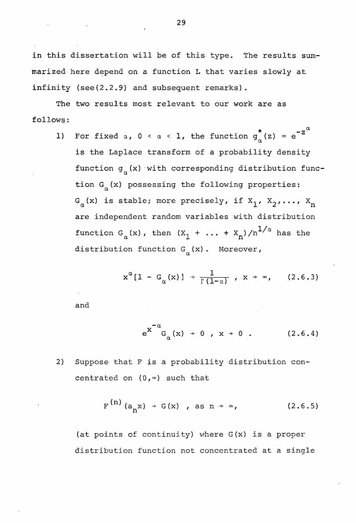
in this dissertation will be of this type. The results sum-
marized here d~pend on a function L that varies slowly at
infinity (see(2.2.9) and subsequent remarks).
The two results most relevant to our work are as
follow~.:
1) * For fixed a, 0 < a < 1, the function g (z) a
a -z = e
is the Laplace transform of a probability density
function g (x) 'with corresponding distribution funca
tion G (x) possessing the following properties: a
Ga(X) is stable; more precisely, if Xl' X2 ,···, Xn
are independent random variables with distribution
function Ga(x), then (Xl + ..• + xn)/nl / a has the
distribution function G (x). Moreover, a
and
-a eX G (x) + ° , x + ° . a
(2.6.3)
(2.6.4)
2) Suppose that F is a probability distribution con-
centrated on (0,00) such that
F (n) (a x) + G (x) I as n + 00 I n
(2.6.5)
(at points of continuity) where G(x) is a proper
distribution function not concentrated at a single

30
point, and F(n) (x) is defined by the equations
and
Then
F (0) (x) = 1
x
F (n) (x) = f F (n-l) (x-s) dF (sl
o
(a) there exists a function L that varies
slowly at infinity such that
X-aLex) 1 - F(x) ~ r(l-a) (2.6.6)
(b) Conversely, if F is of the form (2.6.7),
it is possible to choose constants a n
such that
nL(a ) n
------ + 1 , n + 00, a~
(2.6.7)
and in this case (2.6.5) holds with
G = G • a
Result (2) implies that the possible limits G in
(2.6.5) differ only by scale factors from some G . a
An example of the stable distribution mentioned in re-
suIt (1) is the stable stribution with characteristic

31
exponent a = 1/2 with parameter y defined by
F (x) = 2[1 - ~(a/lx)] y
(2.6.8)
F (x) has probability density function f (x) given by y y
f (x) = ~ x-3/ 2 y I21T
2 -y /(2x) e , x > o. (2.6.9)
* The Laplace transform of f (x) denoted by f (z) is given by y y
(2.6.10)
Unfortunately, explicit expressions for the stable dis-
tributions F (x) have been obtained only for the two cases a
with characteristic exponents a = 1/2 and a = 2, respective-
lye The characteristic function ¢ (z) of the distribution a
function F (x) can be obtained for general a, however, (see a
[19], for example) and is given by
( ) { I I a ( 'ITa •. 'ITa ) (1 )} CPa Z = exp - Z cos2 - J.sJ..n2 sgn z r -a
where a ~ 1 and ¢ (z) is defined by a
00
¢ {z} a =)
(2.6.11)
(2.6.12)

32
Although the asymptotic behavior of certain random var
iables will be of concern in this dissertation, we have
found it more convenient to develop the analysis from the
exact formulae which are obtainable. tiherever applicable,
however, we shall'point out the connection between our work
and the results of this Section.
CHAPTER III
FIRST-PASSAGE TIMES AND MAXlr1A FOR THE RANDOM
WALK WITH NEGATIVE EXPONENTIALLY DISTRIBUTED
INTERVALS BETWEEN STEPS
3.1 Introduction
In this chapter we shall be concerned with the general
class of problems connected with first-passage times. We
say that the particle makes a first passage from state m to
state n during the small time interval (t,t+dt) if S(O} = m,
S(s} ~ n, 0 < s ~ t, and S(t+dt) = n where Set} represents
the position of the particle at time t. The probability of
this event will be denoted by f (t)dt. We define F (t) ron mn
by the equation
F (t) = 1 mn - I a
t
f (x) dx • ron (3.1.1)
Fron(t) is the probability that given S(O) = m, no first pas
sage to n occurs prior to or at time t. The corresponding
Laplace transforms are defined by
co
I -zt
<Pmn(Z) = e o
fmn (t) d t ; <P mn (z) J e -zt = Fmn(t)dt · o (3.1.2)
Intimately connected with the first-passage-time prob-
lem is the problem of the maximum value of set) during the
interval of time (O/t). The expression "first maximum, II
33

34
extensively used by Feller [18] I is perhaps ambiguous. In
deference to ~sage we continue to employ it with the fol-
lowing meaning. Suppose that there exists a time t' in
(O,t) such that:
(i) Set') > 0;
(ii) set') > sex) for 0 =: x < t'; and
(i i i) S (t ') > S (x) for t' =: x =: t.
Then we say that the p~rticle attains its first maximum at
time t' in the interval (O,t). If no first passage to a
positive value (i.e. no first passage to +1) occurs during
(O,t), we say that t' = O.
In the subsequent sections we shall discuss in turn the
topics:
(i) fmn(t), Fmn(t);
(ii) the time of the rth return to zero;
(iii) the number of returns to zero during (O,t); and
(iv) t', the time of the first maximum, and S(t').
Sections 3.2--3.5 deal with topics (i)--(iv) in connection
with the time-dependent unrestricted random walk with neg-
ative exponentially distributed intervals between steps. In
Sections 3.6--3.8 we shall treat topics (i}--(iii) for the
MIMII queuing process described in Chapter I.
The results obtained in this Chapter are of interest
by themselves. In addition, we shall refer to them often
in Chapter IV. For example, it has been demonstrated by
E. Sparre Andersen [1] and [2] in connection with non-time-
35
dependent random walks that a strong relationship exists
between the problem of the maximum partial sum S among S11 v
S2 , • • • ,
state.
S and that of the particle's sojourn in a given n
It will be shown in Chapter IV that an analogous
relationship holds in the case of the time dependent walks
under study here.
We turn now to the discussion of f (t). mn
3.2 First-Passage Time from mto n for the
unrestricted Random Walk with Negative
Exponentially Distributed Intervals between Steps
We now proceed to derive fmn(t) for the case m ~ n.
The case m = n will be considered in Section 3.3. Because
of the assumption that steps to the right and to the left
belong to two independent Poisson streams with parameters
A and ~, respectively, the probability that a positive or
negative step occurs at any time is independent of the
value of Set), the displacement of the particle at time t.
Moreover, a first pas from state m to state n is equiv-
alent to a first pas to a point In-ml units from the
starting point in either a positive or negative direction,
aqcording to whether or not n - m is positive or negative.
Because the particle may move an unlimited number of steps
in either direction, whatever its starting point, the prob-·
ability of moving In-ml steps in a positive or
direction is independent of the fact that S(O) = m. There-

36
fore, for the unrestricted walk we have
(3.2.1)
which implies that
f oCt) = fO (t). n ,-n (3.2.2)
From considerations of symmetry it is evident that fO (t) = ,-n
fO (t) except for an interchange of the parameters, A and ,n
~, of the underlying Poisson distributions. The foregoing
considerations imply that it suffices to consider only
fOm(t) in order to derive the density function fmn(t).
We begin by deriving fOl(t). In order that a first
passage to +1 occur during (t,t+dt), the particle must either
remain at zero throughout (O,t) and take a positive step
during (t,t+dt), the probability of this event being
e-(A+~)t. ldt; or it may remain at zero until a negative
step occurs during the small interval (s,s+ds), the prob
ability of this event being e-(l+~)S ~ds, and then make a
first passage from -1 to +1 in the remaining time t - s
when 0 < s < t. This leads to the equation
t
fOl (t) = Ae-{A+~)t + J - (H]1) S f_l,l(t-s)ds . (3.2.3) ~ e 0
By (3.2.1) we have
t
fOl (t) = " -(A+ll)t + J - (H]1) S f O,2{t-s)ds (3.2.4) Ae ~ e . 0
For n = 2,3, ... , a first passage to n must he preceded by a
37
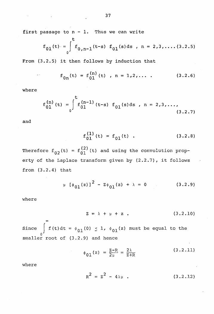
first passage to n - 1. Thus we can write
t
fOl(t) = J f O,n_l(t-5) f Ol (5)ds , n = 2,3, •••• (3.2.5) o
From (3.2.5) it then follows by induction that
n=1,2, •.•. (3.2.6)
where
·t
f~~) (t) = J f~~-l) (t-s) fOl (s) ds , n = 2,3, ••• , o (3.2.7)
and
f~i) (t) = f01 (t) • (3.2.8)
Therefore f 02 (t) = f~f) (t) and using the convolution prop
erty of the Laplace transform given by (2.2.7), it follows
from (3.2.4) that
(3.2.9)
where
Z = A + 11 + Z • (3.2.10)
Since J f(t)dt = ~Ol(O) ~ 1, ~Ol(z) must be equal to the o
smaller root of (3.2.9) and hence
where
Z-R 2A = 211 - = Z+R
(3.2.11)
(3.2.12)

38
From (3.2.6) it follows that
Upon inversion of (3.2.13) using [17), Vol. I, (28), p. 240,
it follows that
fOn(t) = pn/2 nIn {2t/Al1 Je -(A+11)t, n = 1,2, .... , t
where
p = l. II
By symmetry we have
fnO{t) = p-n/2 nln(2t/~ t
-n = p fOn(t)
(3.2 .. 14)
(3.2.15)
(3.2.16)
Equation (3.2.14) has been derived by Feller [19] by extend-
ing a discrete-time result to continuous time with the aid
of conditional probabilities. This technique will be i11us-
trated in Chapter V.
Expressions for FnO(t) arid FOn(t) can be obtained from
(3. 1.1) I (3. 2. 14) and (3.2. 16) and are given by
t -n/2 J -('+1!)x = 1 - np e 1\ t-A In (2x/f"il) dx
o x
-n -'n = 1 - p + p F On (t) •
(3.2.17)
From (3.1.1) I (3.1.2) and (3.2.13) we obtain

39
~On(Z) = 1 - <POn(z)
(3.2.18) ------Z
and
~O ,n+l (z) - 1I0,n (z) = CPOn (z) <POI (z) , (3.2.19)
a result which "'Till be used in Chapter IV. Corresponding
expressions for <PnO{z) and <PnO{z) follow by symmetry.
In order to make use of the asymptotic properties of the
J~function and the modified Bessel function we now proceed to
derive alternate expressions for FOI(t) and F10(t). We do
this by appealing again to Maximon's result given in (2.4.11).
Letting x = At and y = ~t in (2.4.ll), we
t J(At,~t) ~ 1 + J e-(A+~)X [/i;I
1(2x/I;)
o
and
t
obtain
- AIO(2x/Ill}]dx
(3.2.20)
J2(At,~t) = J e-(H)l)X [)lp-l/2 I1 (2x/iil) - AP- 1 I2
(2x/i;)ldX
o (3.2.21)
where J (x,y) is defined in (2.4.1). Upon combining (3.2.20) n
and (3.2.21) with (2.3.9), we find that
t
J(At,llt) - PJ2(At,~t) ~ 1 - pl/2 J e-(H)l)X11 (2x/I;)dx a x
= F01 (t) (3.2.22)
By (3.2.17) and (3.2.22) we have

40
It is clear from (3.2.22) and (3.2.23) that the asymp-
totic properties of the probabilities FOl(t) and FlO(t) can
be deduced from the asymptotic behavior of J (x,y). We can n
deduce the limiting behavior of In(x,y) by the use of equa
tions (2. 4.10), (2.3.2) and (2.4.5). For completeness and
for later use, these results can be summarized as follows:
(3.2.24)
-1 IV (l-p) +
4e -ll (l-/P) 2t [ ()] 2 1/2 r;~) + 0 4~2 ' p> 1,
(l-/P) (21T~) \ <:, '"
where
(3.2.25)
The corresponding result for FO,l(t) follows from (3.2.17).
To obtain asymptotic results for FO (t) and F O(t), ,n n,
it is more convenient to proceed by direct methods rather
than using the results of Chapter II. From (3.2.13) it fol-
10vlS that
J fOn(x)dx = o
n p , p < 1,
= 1, P.2: 1, (3.2.26)

41
and hence
FOn(t) = 1 - pn + J fOn(xldx , p < 1 ,
• t
m (3.2.27)
= J fOn(xldx, p ~ 1 •
t
We need then to determine the asymptotic behavior of
J fOn(x)dx. From (3.2.14) and the asymptotic properties of
t I (x) given in (2.3.2), we have
n
J fOn(x)dx = npn/2 J t t (3.2.28)
as t + 00.
Upon substituting y = x - t and expanding the denominator of
(3.2.28) in powers of (x/t) by means of the binomial expan-
sian, we find that
where ~ and P are defined in (3.2.25).
substituting (3.2.29) into (3.3.37) we obtain

42
n4'n'p (n+l) /2e -~ (l-/p) 2t [ 1 ( 1 )~ 1 - p + ---- --- + 0 --- P < 1
(1-/P) 2 (21TE;) 1/2 (2~) 4~2' ,
(3.2.30) 4 (n+l)/2 -~(I-/p)2t [ (]J
np 2 e 1/2 ·(2l~) + 0 4~2 I P > 1 • (l-/p) (21T~) '" '"
The corresponding results for FnO(t) follow from (3.2.17).
We note from (3.2.30) that FOn(t) tends to 1 - pn for
p < 1 but tends to zero as t ~ 00 when p > 1. Since FOn(t)
represents the probability that first passage to n occurs
after time t, we would expect that it tend to zero with in-
creasing t when p > 1, i.e., when there is a drift of the
random walk toward +00. The result given in (3.2.30) supports
our intuition. On the other hand, when p < I, there is a
drift of the random walk toward -00; and the fact that FOn(t)
tends to a non-zero limit in this case, i.e., there is a non-
zero probability that the particle never passes to +n, is
not surprising. It is also interesting to note that the
n probability 1 - p that passage to +n never occurs tends to
unity as n increases for p < 1. The case A = ~, or p = I,
is particularly interesting, since we would expect no ten-
dency to drift in either direction. We examine this case in
detail next.
When ). = ~, our results take on a pleasing form. From
(3.2.16) we see that fOn(t) = fnO(t) and hence, FOn(t) =
FnO(t) when p = 1. In particular,

43
t
FOn(t) = 1 - n J e-2~x In(2~x}dx o x
(3.2.31)
(3.2.32)
n = 2,3,4, ••• ,
and
(3.2.33)
Equations (3.2.32) and (3.2.33) follow from standard results
for integrals of Bessel functions, given, among other places,
in [37], Section 11,3. From (3.2.32) and (3.2.33) it follows
that
FO,n+l (t) - Fan (t) = e-2lJt
[In (211t) + In+l (211t)] , n = 1,2, ••••
(3.2.34)
From (3.2.32) and the asymptotic properties of the modified
Bessel function of order n given by (2.3.2), we find that
for p = 1, as t ~ 00,
(3.2.35)
From (3.2.35) it is evident that both FOn(t) and FnO(t)
tend to zero as t ~ 00. Since FOn(t) represents the prob
ability that a first passage to +n occurs after time t and
FnO(t) is equal to the probability that a first passage to
-n occurs after time t, we expect, based on (3.2.35), that
the particle eventually makes a first passage to all finite

44
states ±n, n = 1,2, •••• Therefore, in a soccer game between
two evenly matched teams, as described in Chapter I, we would
expect that if the two teams played long enough, we might
eventually witness any given score difference ±n, n = 1,2, ••••
This result is perhaps not intuitively obvious although con-
sistent with the results for the so-called coin-tossing ran-
dom walk discussed by Feller [18], Chapter III.
In order that first passage to both ±n eventually occur,
it is evident that the particle must cross the origin at
least once. This consideration raises the question as to how
fast the path of the random walk oscillates between positive
and negative values. At least a partial answer to this ques-
tion can be obtained by studying the time bet\'leen returns to
the origin, which we shall discuss in the next Section.
3.3 The Time of Occurrence of the rth Return to
Zero for the Unrestricted Random Walk with Negative
Exponentially Distributed Intervals Between Steps
One measure of the nature of the oscillation of the
particle is the a~mount of time which elapses between returns
to zero. We say that a first return to zero occurs at time
t if S(O) = Set) = 0 and S(s) ~ 0, 0 < s < t. We let T r
denote the time up to the rth return to the origin and define
fret) by
f (t)dt = Pr {t < T < t + dt I S(O) = O} . r r
(3.3.1)

45
In this Section we shall discuss the distributional properties
of T which will yield information concerning the time of r
occurrence of the rth tie in a soccer game where S(t), in
this case, represents the score difference between the two
teams at time t. We proceed now to derive fret).
In order that a first return to zero take place at time
t, the particle must take either a positive or negative step
at some time s, 0 < s < t, and then make a first return to
zero from +1 or -1 at time t - s. This fact is expressed by
the equation
t f1 (t) = J {Ae-(HIl)Sf
10 (t-s) + ll e -(HIl)sf
01 (t-s) }ds •
o (3.3.2)
From (3.2.11) and symmetry considerations, it follows that
where
<PI (z)
00
Z-R = -Z-
J e-zt
<P (z) = f (t)dt • r r
o
(3.3.3)
(3.3.4)
and Z,R are defined by (3.2.10) and(3.2.12), respectively.
For integer values of r greater than unity, it is evident
that an rth return to zero must be preceded by r - 1 returns
to zero. Therefore we can write
t
f (t) = J' f (t-s) fl{s)ds r r-l o
(3.3.5)
46
which, by the convolution property of the Laplace transform,
implies that
4> (z) = cp 1(z)CP1(z} , r = 2,3,4, •••• r r-(3.3.6)
By induction, starting from (3.3.3), we have
= (Z-ZR)r = (4A~ )r CPr(z) Z(Z+R) , r = 1,2,3, •••. (3.3.7)
From [17], Vol. I, (28), p. 240, it follows that
f (t) = r(2~)r -(A+~)t r (r-l)! e
t
J (t_s)r-l I (2s~)ds ,(3.3.8) r -o s
r = 1,2,3, .•..
From (3.3.7) we have
dCPr(z) r-l ( ) dz = r(Z;R) ~~~~. (3.3.9)
From (3.3.7) and (3.3.9) we see that
00
4>r(O) ) f (t)dt = (2p) r , p < 1 r
= 1 , p = 1 (3.3.10)
= (2q) r , p > 1
and
E (T ) 00
r ) tf (t)dt ~~ 1 ~T6T = = p < r ~ (l-p)
, r
= 00 , p = (3.3.11)
- 2pr > 1, I- = I P
~ (p-l)
47
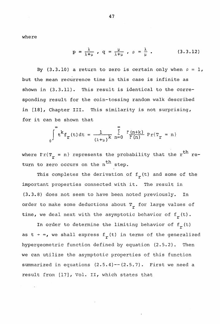
where
p = A~~ I q = A~~ , P = ~ (3.3.12)
By (3.3.10) a return to zero is certain only when p = I,
but the mean recurrence time in this case is infinite as
shown in (3.3.11). This result is identical to the corre-
sponding result for the coin-tossing random walk described
in [18], Chapter III. This similarity is not surprising,
for it can be shown that
= 1 l r(n+k) Pr{T = n} (A+v)k n=O r(n) r
where Pr{T = n} represents the probability that the rth rer
th tUrn to zero occurs on the n step.
This completes the derivation of f (t) and some of the r
important properties connected with it. The result in
(3.3.8) does not seem to have been noted previously. In
order to make some deductions about T for large values of r
time, we deal next with the asymptotic behavior of f (t). r
In order to determine the limiting behavior of f (t) r
as t + 00, we shall express f (t) in terms of the generalized r
hypergeometric function defined by equation (2.5.2). Then
we can utilize the asymptotic properties of this function
summarized in equations (2.5.4)--(2.5.7). First we need a
result from [17], Vol. II, which states that

1 r (m)
48
y
J xn-l(y_x)m-l Jv(ax)dx =
o . r(v+n) (aJv
r (v+l) r (m+n+'v) 2" • (3.3.13)
m+n+v-l [n+v n+v+l • y 2F 3 --2-' 2
m+n+v v+l, 2
2 2 m+n+v+l. -~ ]
2 ' 4 '
where Re(m) > 0, Re(n+v) > 0, and J (x) is defined by equation v
(2.3.4). Equation (3.2.5) implies that (3.3.13) is equiv-
alent to
1 r (m)
o
y
J n-l m-l x (y-x) I (ax)dx =
v r(v+n) v
(~) ym+n+v-l r{v+l)r(m+n+v)
[n+v n+-v+ 1
• 2F 3 -2-' 2 m+n+v m+n+v+l ~]
v+l, 2' 2 4·
(3.3.14)
From (3.3.8) and (3.3.14) we then have
f (t) r
= (2All)r t 2r-l r(2r)
-(A+ll)t F [r r+l 1 2J e 2 3 2' --2-; r+l, r, r+2, Allt •
(3.3.15)
This expression for f (t) is new. Using the asymptotic propr
erties of the generalized hypergeometric function given in
(2.5.4) -
f (t) 'V r
(2.5.7), it follows from (3.3.15) that as t ~ 00,
2 r-
1 r (r+l) r (r) r (r+~) e- lJ (l-/P) 2t + 0 Crt - 5/2) •
r (2r)r{~)r{r;1) !;(All)l/4t 3/2
(3.3.16)
Using induction, or directly using Gamma function formulae,
it can be shown that

49
r (r+1) r {r)T (r+~) ------~~~~~ = . r (2 r) r (~) r (r; 1
) , r = 1,2, ... , (3.3.17)
and, therefore, as t ~ 00, we have
(3.3.18)
To obtain an approximate value for pr{Tr > t} for large
t, we use (3.3.18) and the relation which follows from
(3.3.10), namely,
t
Pr{Tr > t} ~ 1 - J fr(xldx o
= 1 - (2p) r + J t
00
= J f (x)dx . r t
= 1 - (2q) r + J t
00
f (x)dx , p < 1 r
, p = 1
00 (3.3.19)
f (x}dx , p > I, r
where p and q are given in (3.3.12). After integrating
(3.3.l8) by parts and combining with (3.3.19), we obtain
the result
00
- rp-l/4 (l-/Pl (~11/2 J e-y2
/ 2dY +
/2\1 t (1-/P)

50
+ O(t~/2)' p < 1,
-1/4 r-- rp (vp-l) (2)1/2 Joo _ 2/2 - e y dy + 7T
1211 t (l-/P)
+ 0 (rt - 3/2) , p > 1 • (3.3.20)
In terms of a soccer game like that described in Chap-
ter I, Pr{T > t} represents the probability that the time r
up to the rth tie is greater than t. We see from (3.3.20)
that for p ~ I, as t + 00, Pr{T > t} tends to the probabilr
ity that the rth tie never occurs. When p = 1, however,
Pr{T > t} tends to zero as t + 00. Moreover, (3.3.20) shows r
that during a long game of length t between two evenly
matched teams, the probability that the rth tie does not
occur is proportional to rt- l / 2 •
From the form of the Laplace transform of fret} given
in (3.3.7), we conclude that Tr is the sum of r independent
random variables, each having the distribution of Tl with
probability density function fl(t). In order to apply the
results concerning stable distributions described in Section
2.6, the asymptotic form of 1 - Fl(t) = Pr{Tl > t} must

51
be expressible in terms of a slowly varying function L(t)
defined in (2.2.9). From (3.3.20) we see that Pr{T1 > t}
cannot be expressed in this way when p ~ 1, since the neg-
ative exponential function does not vary slowly at 00. On
the other hand, when p = 1, we have
where
1 - F 1 (t) t-1/ 2
= Pr{T1
> t} ~ L(t) r (~)
1 L(t) = i F 1 (t) = v';
t
J f1(x)dx a
(3.3.21)
(3.3.22)
Obviously L(t) = 1/v'; is slowly varying and, therefore, T.J7e
can apply result (2) of Section 2.6 and conclude that when
p = 1, there exist norming constants a r such that
F (a t) ~ GI(t) as r ~ 00, r r
"2 (3.3.23)
I where GI(t) is the stable distribution of order 2" given by
2" (2.6. 8) and
t
Fr(t) = I fr(x)dx a
(3.3.24)
Although the same results do not apply when p ~ 1, it
is interesting to note that the result for p ~ 1 given in
(3.3.20) does contain a term which has the form of the sta
ble distribution of order ~ given in (2.6.8).
52
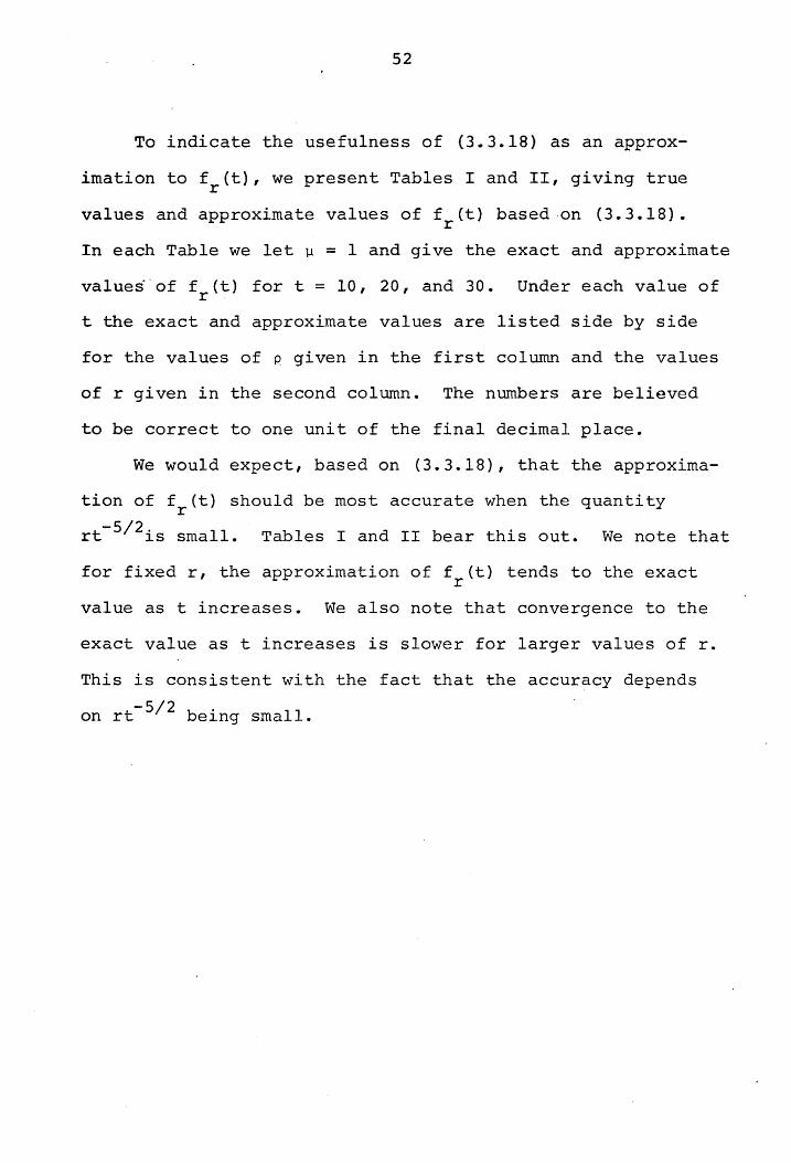
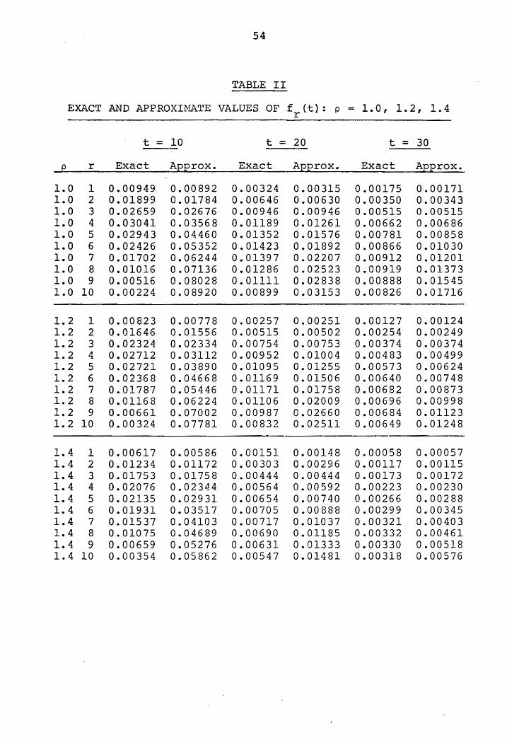
To indicate the usefulness of (3.3.18) as an approx-
imation to f (t), we present Tables I and II, giving true r
values and approximate values of f (t) based on (3.3.18). r
In each Table we let ~ = 1 and give the exact and approximate
values·of fret) for t = 10, 20, and 30. Under each value of
t the exact and approximate values are listed side by side
for the values of p given in the first column and the values
of r given in the second column. The numbers are believed
to be correct to one unit of the final decimal place.
We would expect, based on (3.3.18), that the approxima-
tion of f (t) should be most accurate when the quantity r
rt- 5/ 2is small. Tables I and II bear this out. We note that
for fixed r, the approximation of f (t) tends to the exact r
value as t increases. We also note that convergence to the
exact value as t increases is slower for larger values of r.
This is consistent with the fact that the accuracy depends
on rt- 5/ 2 being small.

53
TABLE I
EXACT AND APPROXI¥iliTE VALUES OF f (t): r p = .6, .8
t = 10 t = 20 t = 30
p r Exact ,AEErox. Exact AEErox. Exact AEErox.
0.6 1 0.00663 0.00609 0.00134 0.00129 0.00043 0.00042 0.6 2 0.01326 0.01219 0.00269 0.00259 0.00087 0.00084 0.6 3 0.01794 0.01829 0.00389 0.00389 0.00127 0.00127 0.6 4 0.01884 0.02439 0.00477 0.00518 0.00161 0.00169 0.6 5 0.01572 0.03049 0.00523 0.00648 0.00187 0.00212 0.6 6 0.01047 0.03658 0.00521 0.00778 0.00201 0.00254 0.6 7 0.00561 0.04268 0.00474 0.00908 0.00204 0.00297 0.6 8 0.00243 0.04878 0.00394 0.01037 0.00195 0.00339 0.6 9 0.00086 0.05488 0.00300 0.01167 0.00177 0.00382 0.6 10 0.00025 0.06098 0.00208 0.01297 0.00153 0.00424
0.8 1 0.00905 0.00843 0.00275 0.00266 0.00132 0.00129 0.8 2 0.01811 0.01687 0.00551 0.00533 0.00265 0.00259 0.8 3 0.02505 0.02531 0.00800 0.00800 0.00390 0.00389 0.8 4 0.02777 0.03375 0.00996 0.01067 0.00498 0.00519 0.8 5 0.02544 0.04218 0.01117 0.01334 0.00583 0.00649 0.8 6 0.01934 0.05069 0.01151 0.01601 0.00693 0.00779 0.8 7 0.01220 0.05906 0.01098 0.01867 0.00663 0.00909 0.8 8 0.00641 0.06750 0.00973 0.02134 0.00655 0.01039 0.8 9 0.00281 0.07593 0.00801 0.02401 0.00619 0.01169 0.8 10 0.00104 0.08437 0.00611 0.02668 0.00559 0.01299
54
TABLE II
EXACT AND APP.ROXINA'rE VALUES OF f (t) : r
p = 1.0, 1.2, 1.4
t = 10 t = 20 t = 30
p r Exact AEErox. Exact AEErox. Exact AEErox.
1.0 1 0.00949 0.00892 0.00324 0.00315 0.00175 0.00171 1.0 2 0.01899 0.01784 0.00646 0.00630 0.00350 0.00343 1.0 3 0.02659 0.02676 0.00946 0.00946 0.00515 0.00515 1.0 4 0.03041 0.03568 0.01189 0.01261 0.00662 0.00686 1.0 5 0.02943 0.04460 0.01352 0.01576 0.00781 0.00858 1.0 6 0.02426 0.05352 0.01423 0.01892 0.00866 0.01030 1.0 7 0.01702 0.06244 0.01397 0.02207 0.00912 0.01201 1.0 8 0.01016 0.07136 0.01286 0.02523 0.00919 0.01373 1.0 9 0.00516 0.08028 0.01111 0.02838 0.00888 0.01545 1.0 10 0.00224 0.08920 0.00899 0.03153 0.00826 0.01716
1.2 1 0.00823 0.00778 0.00257 0.00251 0.00127 0.00124 1.2 2 0.01646 0.01556 0.00515 0.00502 0.00254 0.00249 1.2 3 0.02324 0.02334 0.00754 0.00753 0.00374 0.00374 1.2 4 0.02712 0.03112 0.00952 0.01004 0.00483 0.00499 1.2 5 0.02721 0.03890 0.01095 0.01255 0.00573 0.00624 1.2 6 0.02368 0.04668 0.01169 0.01506 0.00640 0.00748 1.2 7 0.01787 0.05446 0.01171 0.01758 0.00682 0.00873 1.2 8 0.01168 0.06224 0.01106 0.02009 0.00696 0.00998 1.2 9 0.00661 0.07002 0.00987 0.02660 0.00684 0.01123 1.2 10 0.00324 0.07781 0.00832 0.02511 0.00649 0 .. 01248
1.4 1 0.00617 0.00586 0.00151 0.00148 0.00058 0.00057 1.4 2 0.01234 0.01172 0.00303 0.00296 0.00117 0.00115 1.4 3 0.01753 0.01758 0.00444 0.00444 0.00173 0.00172 1.4 4 0.02076 0.02344 0.00564 0.00592 0.00223 0.00230 1.4 5 0.02135 0.02931 0.00654 0.00740 0.00266 0.00288 1.4 6 0.01931 0.03517 0.00705 0.00888 0.00299 0.00345 1.4 7 0.01537 0.04103 0.00717 0.01037 0.00321 0.00403 1.4 8 0.01075 0.04689 0.00690 0.01185 0.00332 0.00461 1.4 9 0.00659 0.05276 0.00631 0.01333 0.00330 0.00518 1.4 10 0.00354 0.05862 0.00547 0.01481 0.00318 0.00576

55
3.4 The' Number of Returns to Zero During (O,t)
for the Unrestricted Random Walk with Negative
Exponentially Distributed Intervals Between Steps
In the previous Section we were concerned with the
distributional properties of Tr' the time of occurrence of
the rth return to zero. In this section we shall discuss
the random variable N(t), which will denote the number of
returns to zero during an arbitrary time interval (O,t).
As an application of our results, we shall be able to give
probabilistic information about the number of ties that
occur during a soccer game of length t. A tie at a given
time s is, of course, equivalent to the event S(s) = O.
First of all, we shall derive an expression for
k (t) = Pr{N(t) = n} • n
(3.4.1)
We do this by using a well known and obvious relationship
between T and N(t), namely, r
Pr{T < t} = Pr{N(t) > n} , n = 1,2,3, •••• n
(3.4.2)
Let K(x,z) denote the Laplace transform of the generating
function of k (t) defined by n
K(x,z) = (3.4.3)

where
= )
56
e-zt k (t)dt • n
As a consequence of (3.4.2), we have
00
l + I xn f e-zt Pr{T
1 xK(x,z) - -z z n
n=l 0
From (3.3.7) it follows that
and hence,
K(x,z) =
where
< t}dt =
1 z
R
1 - x
xK (x, z)
- x
z[Z - x(Z-R)]
Combining (3.4.3) and (3.4.7) we obtain
* R(Z-R)n k (z) = , n = 0,1,2, ••••
n zzn+l
*
,
By (3.4.8) it follows that kn(z) can be written as
(4A 1-1) n+l
ZRZn+l(Z+R)n '
and upon inversion, we obtain
(3.4.4)
(3.4.5)
(3.4.6)
(3.4.7)
(3.4.8)
(3.4.9)
(3.4.10)

k (t) n
and
57
x ( y [ (n-1) , (A +11) (t-x) ] \ r (n-l)
n = 2,3, •.• ; (3.4.11)
x {I - 4 Ally [2, (A + il) (t - x) ] } dx ; (A+ll) 2
t
kO(t) = Pr{T1 > t} = 1 - f f1(x)dx a
(3.4.12)
(3.4.13)
where f 1 (t) is given by (3.3.8) and
t
y[n,t) = f xn - 1 e-xdx a
(3.4.14)
is the incomplete Gamma function.
For the syrmnetric case, i.e., when A = 11, the fact that
y[n-l,t] - y[n+l,t] -t = e ( -I-n-1 tn ) ~(n) + r(n+l) (3.4.15)
implies that
k (t) = n
r(n-1) r(n+1}
J2 il(t-S)] + [211(t-s)] d ( n-l n) r (n) r (n+ 1) s,
n = 1,2,3,.... (3.4.16)

58
To provide a feeling for the probabilities themselves,
we give a numerical table of k (t) for selected values of n
nand t for the case A = p = 1. Each entry in Table III is
the exact value of kn(t) corresponding to the value of t
given ·-at the top of the column and the value of n given at
the beginning of the row. The values are believed to be
correct to one unit of the final decimal place.
It is interesting to observe from Table III that kO(t)
and kl(t) appear to be equal, or nearly equal, for all values
of t. This can be explained by noting from {3.4.9} that for
A = p,
* R2 = kO (z) - --2 •
zZ (3.4.17)
Upon using (3.4.8) and inverting, we obtain
(3.4.18)
where
-21ft E (t) = e to' (1+211t). (3.4.19)
The rapid decrease of E(t) as t increases accounts for the
two probabilities kO(t) and kl(t) being so nearly equal.
For example, for the case 11 = 1, we have E(5) = 4.9 x 10⁻⁴ ,
-10 and E(lO) = 4.3 x 10 •

59
TABLE III
. EXACT VALUES OF k (t): A = 1l = 1 n
t 5 10 15 20 25 30 n
0 0.2637 0.1820 0.1475 0.1273 0.1137 0.1036 ·1 0.2632 0.1820 0.1475 0.1273 0.1137 0.1036 2 0.2203 0.1711 0.1420 0.1239 0.1112 0.1018 3 0.1445 0.1494 0.1310 0.1170 0.1064 0.0982 4 0.0716 0.1192 0.1153 0.1069 0.0993 0.0928 5 0.0267 0.0857 0.0961 0.0943 0.0903 0.0859 6 0.0076 0~0547 0.0754 0.0801 0.0798 0.0778 7 0.0017 0.0307 0.0554 0.0652 0.0684 0.0689 8 0.0003 0.0150 0.0378 0.0508 0.0569 0.0595 9 0.0004 0.0063 0.0239 0.0376 0.0457 0.0500
10 0.0000 0.0023 0.0138 0.0265 0.0354 0.0410

60
To find the moments of N(t), i.e., the quantities de-
fined by
we use the relation
co
co
2 n k Pr{N(t) = n=1
n} ,
J e-zt E{N (t) [N (t) - 1] •.• [N (t) - (k+l)] }dt
o
For example, we find by differentiating (3.4.7) that
(X)
J e-zt E{N(t) }dt =
o zR (Z+R) •
Upon inversion we obtain
t
E[N(t)] = 2~ J e-(HI1)X II (2x~)dx 0
00
(3.4.20)
x=l
(3.4.21)
(3.4.22)
= (I+p) - 1 + 2~ J
- O.+]J)x II (2x~)dx , II-pi
e
t
(3.4.23)
provided that p =. ~ ~ 1. ]J The latter part of (3.4.23) follows

61
from [17], Vol. I, (30), p. 240. Using the asymptotic prop-
erties of the modified Bessel function given in (2.3.2), we
find that, as t + 00,
(l+p) 1 2pl/4 ~ I '-1 E[N(t)] ~ - - {I - ~[~2~t l-vp]} + II-pi Il-IPI
where
and p = ~ t. 1. ~
~(x) = 1
127T
x 2 J e-Y /2dy
-co
When A = ~, (3.4.23) becomes
+ O(~t) (3.4.24)
(3.4.25)
(3.4.26)
which follows from [27], (8), p. 122. Therefore, we have
from (2.3.2) that for A = ~,
E[N(t)] ~~t as t + 00 (3.4.27)
In terms of a soccer game between two evenly matched
teams, (3.4.27) means that over a long period of time t,
the expected nunilier of ties is proportional to IE which in-
creases without bound. We note from (3.4.24), however, that
the expected number of ties between two teams of unequal
62.
(l+p) ability remains bounded above by II-pi - I regardless of how
long they play.
The asymptotic behavior of k (t) and the conclusions n
about a long soccer game drawn froIn this behavior could have
been predicted from the discrete-time random walk results.
For example, it is shown in [18], Chapter III, that in the
symmetric case, the mean number of returns to zero during
the course of n steps is proportional to In for large values
of n. Since the number of steps that occur in (O,t) in-
creases with t, we would expect that the average number of
returns to zero during (O,t) be proportional to IE for
large values of t. Equation (3.4.27) shows that this is the
case. On the other hand, to obtain probabilistic informa-
tion about the number of returns to zero during (O,t) for
small values of t, it is convenient to use the licit for-
mulae given in this Section.
We note that k = lim k (t) can be interpreted as the n n t+oo
probability that exactly n returns to zero occur if the ran
dom walk is allowed to continue forever. Since oJoofl(X)dX
represents the probability that a return to the origin ever
occurs and kl(t) = oftfl(X)dXt where fl(t) is given by
(3.3.8), we should find, based on (3.3.l0), that
p < q ,
= 0 , p = q
= (2q)n(l-2q) p > q

63
A where p = A+~' and q = 1 - p. An application of (2.2.12)
to equation (3.4.9) does yield (3.4.28). For A ~ ~,
(3.4.28) may be useful for approximating the probability that
over a long period of time exactly n returns to zero occur.
3.5 The Time of Occurrence and Magnitude of the First
Maximum for the Unrestricted Random Walk with Negative
Exponentially Distributed Intervals Between Steps
In this Section we use the results of Section 3.2 to
determine the distributional properties of the first maximum
of the unrestricted random walk with negative exponentially
distributed intervals between steps during an arbitrary in-
terval of time (O,t). We let t' denote the time of occur-
rence of the first maximum during (O,t) as defined in Section
3.1. S(t') then represents the magnitude of the first max-
imum. If no first passage to a positive value, i.e., no
first passage to +1, occurs during (O,t), then we say t l = O.
The probability of this event is given by
Pr{t' = O} = FOl (t) , (3.5.1)
where F01(t) is defined by equation (3.1.1). Analogous de
initions and results hold for the first minimum.
Baxter and Donsker [5] have studied the probabi ty
Pr{S(t') < a} for a general process in continuous time with
discrete steps. They have derived the double Laplace trans-
form Pr{S(t!) < a} with respect to t and a and expressed
64
it in terms of a function we;) defined by the equation
(3.5.2)
Unfortunately, application of this result is difficult, and
it seems more convenient to proceed directly in our case.
Thus we can also obtain probabilistic information about t',
the time of occurrence of the first maximum, as well as the
value of Set'). We can then use these explicit results to
obtain asymptotic approximations for large values of t. We
turn next to the derivations of the joint probability and
probability density function that t' = sand Set') = k.
We define mk(s,t)ds as the probability that
(i) Set') = k, k = 1,2,3, ••• ; and
(i i) s < t I < S + ds, 0 < s < t.
In order that set') = k ~ 1, and that the maximum occur for
the first time at time s, 0 < s < t, a
to k must occur at time s followed by no
t passage from 0
passage from
k to k + I during (s,t). Therefore, because of the Markov
property of the Poisson process, we can te
mk (s,t) = fOk (s) FOI (t-s) , 0 < s < t, (3.5.3)
where fOk(t) and FOl(t) are given in (3.2. ) and (3.2.27),
respectively. Evidently,
mk (t It) = f 0 k (t) (3.5.4)

65
and therefore (3.5.3) holds for 0 < s < t.
We define m(s,t) by
m(s,t)ds = Pr{s < t' < S + ds} , 0 < S ! t, (3.5.5)
and i~ follows from the definition of mk(s,t) that
00
m(s,t) = I mk(s,t) • k=l
(3.5.6)
To determine m(s,t} completely, it is necessary to find 00
I fOk(s). By (3.2.13) we have k=1
00 1 I fOk (s) = -2 .
k=l TIl.
1 Je Zs A [ 211 ] Z 1 - Z+R dz , = 2TIi C
(3.5.7)
interchange of summation and integration being justified by
the absolute convergence of the right-hand side of (3.5.7).
Upon comparing (3.5.7) with (3.2.18), we obtain by symmetry
the result
co
I fOk (s) = AF10 (s) • k=l
(3.5.8)
On combining (3.5.6) and (3.5.8), we obtain the elegant for-
mula
m(s,t) = FIO(S) FOI (t-s) (3.5.9)
The similarity of this result to the work of E. Sparre
66
Andersen [1] and [2] for discrete-time random walks, of
which the coin-tossing ga~e described in [18], Chapter III,
is an example, is most striking. Further observations on
this subject will be made in Chapter V.
~rom (3.5.3) it is easy to obtain the probability
Mk(t) = Pr{S(t') = k} , (3.5.10)
for, in order that S(t') = k ~ I, the maximum attained by
the particle during (O,t) must occur for the first time at
some point s, a < s < t. Hence, we have
t
~(tl = J ffik(s,tlds · a
(3.5.11)
From (3.5.3), (3.5.11) and the convolution property of the
Laplace transform, we have
1 21Ti Jezt
~Ok(z) ~Ol(z)dz , C
and from (3.2.19) it follows that
As a consequence of (3.5.13) and the fact that
t
(3.5.12)
(3.5.13)
FO,k+l(tl - FO,k(t) = J [fOk(x)-fOk+l (xl]dx , a
we have
Pr{ S (t I) > k} = I M. (t) = j=k ]
t
J fOk(xldx a
(3.5.14)

67
where fOk(t) is given in (3.2.14). The result given in
(3.5.14) was obtained by Baxter and Donsker [5] using the
Fourier transform method mentioned earlier. The other fi-
nite-time results given in this Section are original as far
as we have been able to ascertain.
In addition to the asymptotic behavior of Mk(t), which
can be deduced from equations (3.2.17) and (3.2.30), it is
interesting to note that Mk(t) has the following stationary
distribution which follows from (2.2.12) and (3.5.12):
k = p (l-p) , p < 1
(3.5.15) = 0 , p ~ 1
The asymptotic behavior of m(s,t) can be deduced from
(3.2.24) for the case A I ~ and from (3.2.35) for the case
A =~. From (3.2.24) we have as s, (t-s) ~ 00,
2 2A(1+/P)e-~(l-lP) s [1 (1)] m(s,t) ~ +0 [nsfil.[] 1/2 (l-iP) [4s/All] 16s 2 All
, p < 1,
- 2 2A (l+IP) e-~ (l-/p) (t-S)[ 1
tv· 1 2 [n(t-s)fil.[J / (/P-l) [4(t-s)v'A1lJ
+ 0 ( 1 )] , 16A~(t-s)2
p > 1, (3.5.16)
and from (3.2.35) we have
1 1 m(s,t) tv , P = 1. n Is (t-s)
(3 .. 5.17)

68
Upon integrating by parts, we obtain from (3.5.16) and
(3.5.17) the result
J t 1/4.r- [ - A a t
m (s ,t) ds tV p ~l+Yp) e __
at In IAat
-At e - --+ IAt
I\" 1 - 2 arc sin ra , p = 1, n
where
-A(l-a)t e
It(l-a)
12A.t 2 .
J e-y /2 ] dy , p<l,
12i\at
(3.5.18)
12At. (I-a) 2 ] IA J e-Y /2dy ,
o
p > 1,
A = 1.1 (1-/p)2 • (3.5.19)
From (3.5.18) we observe that for p < I, 0 < a < 1,
Pr{t' > at} ~ 0 as t ~ 00, i.e., the first maximum has a
strong tendency to occur during (O,at) after which the par-
ticle has a tendency to drift toward -00. On the other hand,
when p > 1, there is a dri toward +00 and in this case,
Pr{t l > at}, 0 < a < 1, approaches a non-zero limit as
t ~ 00. The case p = 1 is especially interesting. We note
from (3.5.17) that the t maximum is more ly to occur
at a time near zero or t as t increases, a result which is
not intuitively obvious. This same phenomenon has been
shown to occur in the coin-tossing random walk discussed in
[18], Chapter III. This similarity to the coin-tossing ran-
dorn i.valk will be discussed in more detail in Chapter V.

69
In terms of a soccer game between two evenly matched
teams, we conclude that the largest score difference during
a very long game is more likely to occur near the beginning
or the end of the game rather than at any time in between.
The results'pertaining to stable distributions are not
directly applicable here. It is interesting to note, how-
ever, the appearance in (3.5.18) of a term which has the
form of the stable distribution of index ~ defined by (2.6.8).
The usefulness of (3.5.18) as an approximation will be
commented upon in Section 4.6.
We turn now to the consideration of first-passage times
for the MIMll queuing process described in Chapter I.
3.6 First-Passage Time from m to n
for the MIMll Queuing Process
A complete analysis of first-passage times and the num-
ber of returns to zero for the queuing random walk is com-
plicated because of the barrier at zero. To derive fOn(t),
for example, one must deal with a more complicated two-bar-
rier problem rather than the one-barrier problem appropriate
to the case of the doubly-infinite random walk. Bailey [3]
has given the Laplace transforms of f (t) for the cases mn
m < nand m > n and obtained explicit results for the case
m > n. Apparently, no explicit formulae for f (t) have mn
been published for the case m < n. A step in this rection
will· be made in this Section. Heathcote [25] has obtained

70
systems of equations relating f +l{t) for the GI/M/l queue m,m
(defined in Chapter I), but no explicit formulae for MIMll
seem to be obtainable from Heathcote 1 s work.
There are also no published results concerning the time
of occurrence of the first maximum, or maximum number of cus-
tomers present during an interval of time of arbitrary length
t. Cohen [8], however, has obtained expressions for the dis-
tribution of the maximum number of customers present during
a busy period for the MIGll and GIIMll queues.
We now proceed to derive fmn(t), the probability den
sity function of first passage to n at time t given S(O) = m.
In the sequel the most useful results will be the expressions
As before, we let
Pmn(t) = Pr{S(t) = n I S(O) = m} (3.6.1)
where Set), as re to the queuing process, represents
the number of customers in the system at time t. The Laplace
transform of p (t) is defined by mn
TI (z) ron e- zt p (t)dt. ron (3.6.2)
Explicit expressions for p (t) were first given by A.B. mn
Clarke [7]. Using a difference equation technique, Conolly
[9J found that

where
A m =
1T (z) m,n
1 Ji\ ' a R
B m =
=
=
71
A a. n + m
c en m
(1- S) m (a.-I) a R
B an , n m
, n
< - m,
> - m,
+ B m
(3.6.3)
• (3.6.4)
The letters a,S denote the larger and smaller roots, respec-
tively, of the quadratic equation
2 ~x - Zx + A = 0 , (3.6.5)
where
2 2 Z = A + ~ + z , R = Z - 4A~ (3.6.6)
Let umn(t)dt denote the probability that during
(t,t+dt) the system passes to state n given that S(O) = m,
and let
* u (z) = mn
o
00
J e -zt u (t)dt. mn (3.6.7)
The passage to n during (t,t+dt) may be the first or else
a first pass to n has occurred at some time s, 0 < s < t,
followed by a passage to n at time t - s given S(O) = n.
Accordingly, it follows that
t
umn(t) = fmn(t) + J fmn(s) unn(t-s)ds • o
(3.6.8)

72
Using (3.6.8) and the convolution property of the Laplace
transform, we find that
* <P (z) = ron
u (z) mn (3.6.9)
* I + unn (z)
Taking a different point of view one can think of the
probability of a passage to n during (t,t+dt) as the prob-
ability that at time t there are n - 1 or n + 1 customers in
the system and during the 110wing small interval (t,t+dt)
an arrival or departure occurs. Hence, we can write
* u (z) = A1T l(z) + l1A +l(z), n = 1,2, ••• , (3.6.10) mn m,n- m,n
and
* umO (z) = 111T m, 1 (z) , m = 0, l, 2 , • • • • (3.6.11)
Using the quadratic relation given in (3.6.5), together with
equations (3.6.3) and (3.6.10), it follows that
u* (z) = Z[A an + Ben] n < m, mn m m '
= 2AA a n - 1 + ZB en n n
, n = m, (3.6.12)
, n > m.
In the same manner we obtain from (3.6.11) equation
* umO(z) = l1[A a + B S] , m = m m 1 I 2 I • • • ,
(3.6.l3)
, m = O.

73
From (3.6.9) we have
<I> (z) 1 = ron m-n
, rn > n > 1, a
m· Sm (1- S) } n-m {a (a-I) + = p
n Sn(l-S) a (a-I) + , rn < n,
(3.6.14)
Also,
<l>mO (z) -m 1 , 2 ,3, . . . , = a m =
Aa- l (3.6.15) 4>OO(z) = . A+Z
Using [17], Vol. I, and equations (3.6.14) and (3.6.15), we
have
- (A+l.l) t fmn(t) = p-(m-n)/2 e t (m-n) I (m-n) (2t/Al.t) , rn > n > o.
(3.6.16)
The function f 10 (t) is the classical busy period density for
the MIMll queue. Equations (3.6.14) - (3.6.16) have been
given by Bailey [3].
When m < n, ¢ (z) does not seem to be invertible in mn
terms of known tabulated functions although it possesses an
elegant form. For the case A = ~, however, an inverted form
does exist although it is somewhat formidable. To see this,
consider <I> (z), m < n, as given by (3.6.14). In this case, mn

74 .
as = 1, and we have
<Pmn (Z) (3.6.17)
Upon inversion of (3.6.17) we find that
(3.6.18)
where
ak = (2n+1)k + n - ro • (3.6.19)
Equation (3.6.18) has not been published previously.
Further light shed on the problem if one considers
the equation relating f (t) and f 1 (t) for n > ro, mn n- ,n
namely,
t
f (t) = mn J f 1 (s) f (t-s)ds · m n- n-l, n o ,. (3.6.20)
Therefore, we could derive f (t) recursively if we knew the ron
form of f 1 (t). The functions f 1 (t) and f +l(t) n- ,n n- ,n n,n
are related by the equation
t
+ ~J e-(~+~)sf 1 (t-s)*f 'l(t-s)ds, n- ,n n,n-r o
f (t) "\e-(~+ll)t +1 = A n,n
(3.6.21)
and hence,
00
<Pn,n+l{Z) = 1 - ~ 9n-l,n(z)
= ~ L j=O
[
ll¢ (Z}]j n-1~n (3.6.22)

75
which implies that
t f (t) = Ae-(A+~)t + A ~ J (~s)j -(A+~)sf(j) (t-}d n,n+l L JO
, e n-l,n S S. j=Oo .
(3.6.23)
-At Therefore, since we know fOI{t) = Ae , we could derive
f +l(t) recursively using (3.6.23), albeit a cumbersome n,n
process. For example, f 12 (t) is given by
t
f12
(t) = Ae-(Hlllt + A~ e- At J e-lls'A:s I1
[2!A\ls(t- s l]ds • o
(3.6.24)
Equation (3.6.23) appears to be new.
An explicit solution in terms of known functions can
be obtained from the integral equation given by (3.6.8). In
fact, it is easily verified that
00
= u (t) + L (_l)k u (t) * u (k'ct) mn k=l mn nn
(3.6.25)
satisfies (3.6.8). From (3.6.10) and (3.6.l1) we see that
u (t) can be expressed in terms of the state probabilities ron
Pmn(t) which are known (see [30], Chapter I, for example).
Explicit expressions for f (t) are not easily obtained from mn
(3.6.25), however.
3.7 The Time of Occurrence of the rth Return
to Zero for the M/M/l Queuing Process
We now consider fret) for the M/M/l queue where

76
f (t)dt = Pr{t < T < t + dt I 5(0) = O} r r
(3.7.1)
and T denotes the time of occurrence of the rth return to r
zero in the queuing random walk. In this case the random
variable T represents the amount of time which elapses ber
fore the server becomes idle for the rth time. Throughout
this Section we assume that S(O) = 0, i.e., the server is
idle at time t = O.
From (3.6.1S) we have
tPl(z) = ex (1.+11) (3.7.2)
where
00
(3.7.3)
and ex is the root of (3.6.S) with greater absolute value.
As in the unrestricted random walk, we have
t
and hence,
fr(t) = J fr_1(t-s) f1(s)ds , a
Upon inversion, equation (3.7.S) yields the result
f (t) r =
r(2AP)r/2 (r-l) !
t -),t J -~s r-l e' e [t-s] Ir(2s~)ds
o S
(3.7.4)
(3.7.S)
(3.7.6)
77
We note that
~l(O) = 1 , p < 1, (3.7.7)
1 = , p > 1, p
and, therefore, a return to zero is certain only when p ~ 1.
Differentiating ~l(z) we find that the expected value of Tl
is given by
E (t) 2 = II (l-p) , p < 1,
(3.7.8)
= co , p > 1,
where p = Alp- We note that in the case p = I, a return to
zero is certain; but, according to (3.7.8), the mean recur-
renee time is infinite, a phenomenon which appeared in con-
nection with the unrestricted random walk as well.
Sinqe Tr represents the sum of r mutually independent
random variables each distributed as TI' we can examine the
behavior of 1 - ftfl(X)dX as t + 00 to determine whether or o
not the theory of stable distributions given in Section 2.6
is applicable. From (3.7.6) it is not difficult to show
that
where
t
F1(t) - J f1(x)dx o
(3.7.9)

78
t
F11 (t) = -1/2 f -(H\1)s II (25 n:;) ds p e . I
a s
and
t
FI2
(t) = -1/2 e-
At J -llS II (2s n:;) ds p e 0 5
By (3.7.7) and [17], Vol. I, (4), p. 195, we have
Therefore we conclude that
and that
lim F12 (t) = 0 , t-roo
(3.7.10)
(3.7.11)
(3.7.12)
(3.7.13)
(3.7.l4)
From (3.7.10), (3.7.12), and (2.3.2) it then follows that
00
p < 1,
rv--,p 1 = 1. (3.7.15)
We note from (3.7.15) that for p < 1, the limiting form of

79
1 - Fl(t) is not expressible in terms of a slowly varying
function L (t) defined in (2.2.9). Therefore -the resul ts of
Section 2.6 do not apply. We note, however, that the lim
iting form of 1 - Fl(t) for the case of p < 1 is expressible
in terms of the stable distribution of index ~ given by
(2.6.8). For p = 1, however, we see from (3.7.15) that
where
L(t) 1 - F1(t) 'V
rtr(1/2)
L(t) = 1
I; I
(3.7.16)
(3.7.17)
and is slowly varying. Therefore we can apply result (2)
of Section 2.6 and conclude that for p = 1, there exist norm-
ing constants a r such that
F (a t) + G1(t) as r + 00 , r r _ 2
(3.7.18)
where Gl{t) is the stable distribution of index 1 given by
2" (2.6.8) and
t
Fr(t) = J fr(x)dx o
(3.7.19)
3.8 The Number of Returns to Zero
During (O,t) for the MIMl1 Queuing Process
In the queuing s, the number of returns to zero
during an arbitrary of time (O,t) can be inter-
80
preted as the number of times the system becomes empty, i.e.,
the number of times the server becomes idle.
As before, we let N(t) denote the number of returns to
zero during (O,t) and define the probability
Evidently,
k (t) = Pr{N{t) = n I S(O) = O} • n
t
kO(t) = pr{T1 > t} = 1 - J f1(s)ds o
(3.8.1)
(3.8.2)
To derive k (t), n = 1,2,3, ••• , we follow the same n
steps as we did in Section 3.4 for the unrestricted random
walk utilizing the relation
Pr{T < t} = Pr{N(t) > n} • n
(3.8.3)
We define K(x,z), the Laplace transform of the generating
function of kn(t), by equation (3.4.3). We can then use
equations (3.4.5) and (3.7.5) to find that
; [l - 2A ~ ]
K (x, z) = (A +z) (Z+R)
(3" 8.4) [1 - 2 A lJX ] .
(A+Z) (Z+R)-
Upon expanding (3.8.4) powers of x, we observe that
* = ~ [((A+~)ar- ( A t+l] k (z) 1I+z)~ •
(3.8.5) n

81 .
Upon inversion we obtain
(3.8.6)
where
t -n/2 ( ) = ...,.n.:-p ___ ...---
An t (n-l) ! J e-O.+Jl)Y y[n,A(t-y)l I n (2y!>:];")dy , (3.8.7)
o
and
t
y[n,t] = ) -x n-l e x dx. (3.8.8)
From (2.2.11), (2.2.12), and (3.8.5), we conclude that k (t) n
has the stationary distribution given by
k = 0 n
where p = ~ and k = lim k (t). ~ n t~oo n
, p .:: 1,
(3.8.9)
For the queuing process we refer to p = (mean arrival
rate) / (mean service rate) = It - as the traffic intensity. 1.1
From (3.8.9) we see that as t ~ 00, the probability that the
server becomes idle a finite number of times tends to zero
when the traf c intensity p does not exceed unity.
Upon application of (3.4.21) to (3.8.4), we find that
t E[N(t)l = J e-(A+Jl)X Y np-n/2 In(2X~)dx
o ,n=2 x (3 .. 8.10)

82
For p = I, (3.8.10) becomes
211 t
E[N(tll = J e-x [11(xl + 12 (xDdx • a
(3.8.11)
The integral in (3.8.11) can be evaluated (see [27], p. 122,
for example,) to obtain for p = I,
By using the asymptotic properties of the modified Bessel
function given in (2.3.2), we find that as t ~ 00,
E [N (t II '" 4 # , p = 1. (3.8.13)
We conclude that when the traffic intensity is equal to
unity, the expected number of returns to zero is proportional
to t l/2 as t ~ 00 although the expected length of time be-
tween returns is infinite. This result suggests that it may
be possible even when p = 1 to find an asymptotic approx-
imation to the probability that the fraction of an interval
during which the server is busy is equal to a, a < a < 1.
Such a result does exist and wi be derived in Chapter IV.
This concludes our discussion of the number of returns
to zero during an arbitrary time interval for the MIMII
queuing process.

CHAPTER IV
SOJOURN TIME PROBLEMS
4.1 Introduction
In Chapter III we were concerned with the amount of time
required for the particle to pass from one state to another.
In this Chapter we shall be concerned with the proportion of
an arbitrary time interval of length t that the particle
spends in a given state. For example, in the queuing process
one may wish to know what proportion of time the system is in
state zero, that is, what proportion of time the server is
idle. A state T will consist of a set of integral valued
real numbers since we assume in the random walks under con-
sideratiop that the particle moves in unit steps. We say
that the particle is in state T at time t if Set) E T where
Set} denotes the position of the particle at time t. For
any state T, let XT(t) be a random variable such that
(4.1.1)
= 0, Set) t T.
The sojourn time 0T(t) in state T is then defined by the
equation
t
°T(t) = f xT(x)dx o
83
(4.1.2)

84
and represents the amount of time the particle spends in
state T during the time interval (O,t).
From the structure of the random walks described in
Chapter I, it is evident that an infinite number of states
could pe defined. Good [23] has studied the general problem
where n possible states are considered. Tak~cs [34] has
derived some general results for the two-state sojourn
problem. The stochastic process which alternates between
two possible states, A and B, is sometimes called an alter
nating renewal process. Such processes are discussed in
[13], Chapter VII. In this Chapter we shall deal only with
two and three state problems, that is, we will be concerned
only with time spent in two or three possible disjoint
states. We shall obtain general and specific results for
cases of particular interest in the unrestricted and queuing
random walks. Further references to specific results by
Good, Tak~cs and others will be made in the appropriate
Sections.
In the next Section we shall derive a general expression
for the two-state sojourn distribution and density functions.
This will be followed, in Sections 4.3 - 4.5, by applications
of this general result to both the unrestricted and queuing
random walks. The three-state sojourn problem will be dis
cussed in Section 4.7.
In Section 4.6 we shall give numerical results with the
objective of assessing the effectiveness of the asymptotic

85
approximations derived in Sections 4.3 - 4.5 and to compare
our results with those of Takacs where possible. We note
that the asymptotic formulae given in this Chapter will
frequently be expressed in terms of the stable distributions
discuased in Section 2.6. This is perhaps not surprising
since the sojourn time in a given state is the sum of dis-
joint intervals of time spent in that state. Therefore we
might expect that the stable laws which govern the asymptotic
behavior of sums of random variables would influence the
asymptotic behavior of the sojourn time distribution. In
fact, this is the point of view taken by Takacs [35] and the
asymptotic distributions for sojourn times obtained in his
work are based on the theory of stable distributions. We ~
shall discuss in Section 4.6 the usefulness of Takacs
approach to asymptotic results, contrasting it with the
exact asymptotic approximations obtainable from our precise
solutions to the problems investigated.
4.2 General Solution for the
Two-State Sojourn Time Problem
In this Section we assume two possible states A and B,
i.e. at any time t, either S{t) € A or S(t) E B and there is
no other possibility. We let
p~k) (s,t)ds = Pr{s < 0B
(t) < s+ds[S(O) = k} (4.2.1)
and

86
p~k) (s,t) = pr{oB(t) :: sIS(O) = k}, (4.2.2)
the range of k being the set of all integers for the unre
stricted walk while for the queuing walk, k must be a non
negative integer. The probabilities pik ) (S,t) and plk) (s,t)ds
are defined analogously. The absence of any superscript k
in (4.2.1) and (4.2.2) will be understood to mean S(O) = o.
We let TAB denote the first-passage time from A to B,
i.e. TAB = T if S (to-dt) E Bi S (to+x) E A, (0 ~ x < -r); and
S(to+-r) E B. Then let
G(t) = pr{TAB
< t} (4.2.3)
and
g(t)dt = Pr{t < TAB < t+dt}. (4.2.4)
Analogous expressions for state B will be denoted by TBA ,
R{t) and h{t), respectively.
We shall assume that the distributions of TAB and TBA
depend only on the fact that a transition is made from B
to A or vice-versa, i.e. the Markov property holds. Under
this assumption general expressions for PB(s,t) and PB(s,t)
will be derived. It should be remarked that these results
could be obtained as a special case of the three-state
sojourn problem to be considered in Section 4.7. It is more
convenient and more instructive, however, to derive the two-
state result first.
We begin by obtaining expressions for p~k) (s,t) and

87
p~k) (s,t). The corresponding expressions, pik ) (s,t) and
pik ) (s,t), for state A can then be obtained by use of the
relationships
(4.2.5)
and
(4.2.6)
Equation (4.2.5) follows from the fact that at any time t,
either Set) E A or else set) E B, and (4.2.6) follows direc-
tly from (4.2.5) by differentiation.
For convenience we assume that S(O) = a and that a
transition from state B to state A has just occurred. To
avoid having to enumerate all the possible cases, the general
results for S{O) = k will be derived in subsequent sections
for the particular cases considered.
Since the particle begins its walk in state A, it can-
not remain in state B throughout the entire interval (O,t).
Consequently,
pr{aB(t) = tls(O) = a} = O. (4.2.7)
In order that aBet) = 0, we must have lAB> t and hence
Pr{aB(t) = OIS(O) = O} = I-G{t). (4.2.8)
We now proceed to derive an expression for PB(s,t)
assuming 0 < s < t. At time t, either Set) E A or set) E B.
Since the particle may leave and re-enter state B more than

88
once during the time interval (O,t), aBet) represents the
sum of disjoint intervals of time during which the particle
remained in state B. Accordingly, let us define un(s,t)ds
as the probability that
(i) S (t) E: Ai
(ii) aBet) is composed of n disjoint intervals of time
during which the particle remained in state Bi and
( iii) s < a B (t) < s +d s •
Similarly, we define v (s,t)ds as the probability that n
(i) S (t) E: B;
(ii) aBet) is composed of n disjoint intervals of time
during which the particle remained in state Bi and
(iii) s < aB
(t) < s+ds.
We begin by considering ul(s,t). In order that Set) E: A,
and aBet) consist of one interval of time of duration s, there
must be an initial period during which the particle remains
in state A followed by an interval of length s during which
the particle in state B while in the remainder of
the interval (O,t) the particle is in state A. Consequently,
U1 (S,t) = J:-Sg(X)h(S) [1 - G(t-s-x)]dx
(4.2.9)
= h (s) {G (t-s) - G (2) (t-s) }
where G(n) (t) is defined by the set of equations

89
G(O) (t) = 1,
G (1) (t) = G(t), (4.2.10)
G(n) (t) = I: G(n-l) (t-s)g(s)ds, n = 2,3,4, ••••
Since the distribution of TAB depends only on the fact that
a transition from B to A has just occurred, we see that when-
ever a transition from B to A occurs, the initial conditions
assumed above are duplicated. Consequently, we can write
u 2 (s,t) as
u2
(s, t) = It-Sg(X)dX IS h(y)u1(s-y,t-y-x)dy x=o y=O
(4.2.11)
= h (2) (s) {G (2) (t-s) - G (3) (t-s) }
where hen) (t) is the n-fold convolution of h(t) with itself
and is defined by the set of equations
h ( 0 ) (t) = 0,
h (1) (t) = h.(it) , (4.2.12)
hen) (t) = J>;S)h(n-l) (t-s)ds, n = 2,3,4, ••••
In general it follows that
u (s I t) n
= Jt~Sg(X)dX JS h(y)un_1(s-y,t-y-x)dy. (4.2.13) x=O y=O

90
If we assume that
u. (s,t) = h(j) (s) {G(j) (t-s) - G(j+1) (t-s)}, j = l,2, ••. ,n-1, J
then we obtain from (4.2.9) and (4.2.13) by mathematical
induction that
un (s,t) = h (n) (s) {G (n) (t-s) - G (n+l) (t-s) },
n = 1,2,3, ••.. (4.2.14)
The expression for v (Sit) is derived in a similar n
manner. Upon following the steps analogous to those followed
in the derivation of (4.2.14) we find that
and
VI (Sit) = g(t-s) [l-H(s) ]
n = 2,3, •.• ,
V (s, t) = 9 (n) (t-s) {H (n-1) (s) - H (n) (s) }, n
n = 1,2,3, .•. ,
(4.2.15)
(4.2.16)
(4.2.17)
Since the probabilities expressed by un(s,t)ds and
vn(s,t)ds account for all possible time spent in state B,
provided 0 < s < t, we conclude that
00
PB (s , t) = L {un (s, t) + v (s, t) } • n=l n
(4.2.18)

91
From equations (4.2.9), (4.2.l3), (4.2.15) I and (4.2.16), it
then follows that
PB (S,t) = h(s) {G{t-s) - G (2) (t-s) } + g(t-s) {l - H{s) } .+
(4.2.19)
and from (4.2.14), (4.2.17) and (4.2.18) we have
PB{s,t) = co
L {h (n) (5) [G (n) (t-s) - G (n+l) (t-s)] + n=l
+ 9 (n) (t-s) [H (n-l) (s) _ H (n) (s) ] },
o < s < t. (4.2.20)
Upon rearranging the terms of (4.2.20) it is not difficult
to show that PB{s,t) is the derivative of
PB(s,t) = co
I H (n) (s) [G (n) (t-s) - G (n+l) (t-s)] n=O
(4.2.21)
and that PB(s,t) satisfies the equation
PB(s/t) = 1 - G(t-s) +
+ J:-Sg(XldX J:h(Yl (s-y,t-y-x)dy. (4.2.22)
Good [23] has given an expres corresponding to
(4.4.20) for the n-stateprob1em in terms of a multiple

92
contour integral. Good assumes, however, that the infinites-
imal transition probabilities, Pr{S(t+dt) £ BIS(t) £ A} and
Pr{S(t+dt) £ AIS(t) £ B}, are constant, i.e. independent of
time. Our assumptions do not eliminate the possibility that
these transition probabilities are time dependent and in
this sense the results given here are more general than
Good's results. Equation (4.2.21) has been obtained by ;
Takacs [34] using an argument similar to, but more obscure
than, the arguments used to derive (4.2.20). The expressions
given in (4.2.20) and (4.2.21) could be obtained directly
from the integral equations (4.2.19) and {4.2.22} using an
iterative procedure. The underlying probabilistic aspects
of the sojourn distributions are more clearly illustrated,
however, by the derivation g'iven in this section. We now
turn to some particular cases.
4.3 Strictly Positive Sojourn Time for
the Unrestricted Random Walk with Negative
Exponentially Distributed Intervals Between steps
In this Section we shall say that the particle is in
state A at time t if Set} ~ 0 and in state B if Set) > O.
The particle passes from state A to state B when a transition
from 0 to +1 is made and from B to A when a passage from +1
to 0 occurs. Therefore, the time required for the random
walk to pass from state A to state B after entering state A
is, in the terminology of Chapter III, the first-passage
93
time from 0 to +1. Similarly, the time required to pass from
state B to state A is equal to the first-passage time from
+1 to O. In the notation of Chapter III, we have then
get) = f 01 (t) (4.3.1)
and
h(t) = flO(t) (4.3.2)
where fOl(t) and f 10 (t) are given in (3.2.14) and (3.2.16),
respectively.
and
Thus, from the results of Section 3.2, we have
2 -(A+ll)t g(n) (t) = pn/ e nI (2t~),
n
h en) (t)
t
= p-n/2e -(A+l-l)tnI (2t~), n
t
(4.3.3)
(4.3.4)
where p = 1../11-
From equation (3.2.11) and symmetry considerations we
have
g*(z) <POI (z) Z - R (4.3.5) = =
211
and
h* (z) <P10 (z) z - R (4.3.6) = =
21..
where
Z = A + 11 + z, R2 = z2 - 41..111 (4.3.7)

94
~mn(Z} is defined by equation (3.1.2), and g*(z) and h*(z)
denote the Laplace transforms of get) and h(t), respectively.
Upon combining the above equations and using the convo-
lution property of the Laplace transformation together with
equatipn (4.2.20), it follows that
PB
(s, t) (4.3.8)
f u(t-s) n }
• e [<PlO(u)] 1>Ol(u)du + Cl
where Cl , C2 are Laplace inversion contours in the u,v planes,
respectively, and 1>mn(z) is defined by (3.1.2). From (4.3.5)
and (4.3.6) it is not difficult to show that I <POl(z) \< 1 and
l~lO(z) I < 1 for Re(z) > O. Therefore it follows from (4.3.8)
that
PB (5, t) 1 f u(t-s) = ---- 2 e ¢Ol(u)du (21fi) C
1 f
vs e ·
C2
(4.3.9)

95
Upon making the substitutions u +, A +11 = (A11)1/2(ex + e-x )
and v + A + 11 = (All)1/2(eY + e-Y), we obtain
and
iP01(u)
1/2 -x = p e ,
-x e
= -1/2e -y p ,
-y e
(4.3.10)
(4.3.11)
When these expressions are substituted in the integrand of
(4.3.9), it follows inunediately that
<Po 1 (u) [ <PIO (v) ¢ 0 1 (u) + til 1 0 (v) ]
1- <POI (u) ~10 (v) (4.3.12)
Using the inversion properties of the Laplace transform,
it then follows from (4.3.9) and (4.3.12) that
(4.3.13)
where F 01 (t) and F10(t) are given by (3.2.17).
Various forms of (4.3.13) may be obtained by making use
of the expressions for F01{t) and F10 (t) given by (3.2.17),
( 3 . 2 . 2 2), and ( 3 . 2 . 2 3) .
We note that the result for PB(s,t) given by (4.3.13)
coincides with the expression for m(s,t) given in (3.5.9).
This suggests an analogy to the "coin-tossing" results in

96
[18], Chapter III. Further reference to this analogy will be
made in Chapter V.
We note that in the symmetric case, i.e., when A = ~,
we have
~ () = <P (z) = 1 _ [Z-R] 01 z 10 z 2~z (4.3.14)
which", after appropriate algebraic manipulation, becomes
(4.3.15)
Hence, with the aid of [17], Vol. I, (3D), p. 240, we find
that
and therefore, when A = ~, we have from (4.3.13) and (4.3.16)
that
PB (s, t)
o < s < t. (4.3.17)
Corresponding results for state A follow from (4.2.5) and
(4.2.6) •
In the foregoing we have assumed that S(O) = O. Suppose
now S(O} = k where k = 1,2,3, .•.. To find p~k) (s,t) we ob
serve that
(k) IS (0) PH (s,t) = f kO (s)F Ol (t-s) + afkO (X)PB (s-x,t-x)dx. (4.3.18)

97
Equation (4.3.18) follows from the fact that after accounting
for the first-passage time from k to 0, the process renews
itself as if it were beginning again in state zero. Using
(4.3.13), (4.3.18) and the convolution property of the Laplace
transform, it follows that
(4.3.19)
the latter expression having been obtained with the aid of
equation (3.2.19). Now since ¢lO(z) satisfies the quadratic
equation given by {3.2.9}, it follows that
k = 1,2, .••• (4.3.20)
Equation (4.3.19) can then be rewritten as
p~k)(S,t) = AFIO(S)F01(t-s), k = 0,
(4.3.21)
= ]..IF 0 1 (t-s) [Fk,O (s) - Fk-1,O (s)],
o < s < t, k = 2,3, ... ,
where F oCt) is given by equation (3.2.17). The exact n,
expressions for p~k) (S,t) given in (4.3.21) are apparently
98
new.
As in the case for S(O) =0, it follows that
Pr {aB (t) = 0 1 S (0) = k} = F 01 (t) , k = 1, (4.3.22)
= 0 , k = 1,2, •.. ,
, k = 0,
(4.3.23) = FkO(t) k = 1,2, •.•.
Analogous results hold for the cases k = -1, -2, •..•
During the interval (O,t) the particle must spend some,
none, or all of the-time in state B. Therefore we expect
that
t (4.3.24)
= k} + J p~k) (s,t)ds = 1 • o
Combining equations (4.3. 2l) _. (4. 4.23), (3. 2.18), and (3.2. 9) ,
we see that for k = 0,
00
J e - z t Pr { 0:: a B (t) :: t } d t = q; 01 (z) [1+ HI 0 (z) 1 o
1 = - I (4.3.25) z
which implies that (4.3.24) holds. That equation (4.3.24)
remains true for k = 1,2,3, ... is verified in a similar
manner.
From the foregoing results we can also deduce the re-
suIt for the more general situation where the random walk is

99.
said to be in state A at time t if s (t) .:s n, and in state n
Bn otherwise. We assume for convenience that S (O) = 0 and
n = 0,1,2, •••• Then PB (s, t) is given in (4.3.21) . For 0
n = 1,2,3, .•. , we observe that after a first passage to n is
made, the problem reduces to that of the positive sojourn
time considered in the beginning of this section. That is,
PB (s,t) satisfies the equation n
PB (s, t) n
(4.3.26)
where p~O) (s,t) is given in (4.3.21). Substituting the result o
for PB (s,t) into (4.3.26) yields o
(4.3.27)
This completes the derivation of p~k) (s,t) and the re
lated probability density function PB (s,t). These results n
give probabilistic information about the proportion of time
during a soccer game of length t that one team remains in
the lead. To obtain similar information about a long
soccer game, we may examine the asymptotic behavior of
p~k} (s,t). Because of the similarity of the discrete-time
random walk discussed in [18], Chapter III, to the continuous-
time walk considered here, we would expect the asymptotic
results to be similar to those for the discrete-time walk.
In particular, for A = ~, we expect distribution of

100
aBet) to follow a so-called arc sine law. This is the case
as will be shown in the following.
(0) Since m(s,t) = PB (s,t), the asymptotic results of
(k) Section 3.5 apply. To obtain asymptotic results for PB (s,t),
we can apply the results obtained in Section 3.2. From
equations (3. 2 • 30), (3.5.16), (3.5 .17), and (4.3.21) , it
follows that for fixed A, ~, as t-s, S~OO,
P~ 0) (s, t)
+ o( 1 2)J, p < 1, 16A~s
1 1/2 'IT[s(t-s)] , p
( 1 )] + 0 2 ' 16All(t-S)
= 1.
r. 1 + L( 4slIl7)
(4.3.28)
[ 1 +
[ 4 (t - s) 1Il7]
p > 1.
(1) -1 (0) By (4.3e21), PB (s,t) = P PB (s,t) and therefore its
asymptotic behavior can be deduced from (4.3.28). For
k = 2,3,4, ... , we have

101
1- 2 ( k) 2 A (1+ fa) (\ - (k -1) ./ 2e -].l (1- p) s
PB
(s,t) ~ ~ ~ x [slfil] 1/2
[ 1 (1 J~ x + 0 2 ' (4s~) 16A].ls
p < 1,
1
n/s (t-s) , p = 1,
(4.3.29)
1- 2 2A (1+/p) p -ke-lJ (1- p) (t-s) ~ x
In[ (t-s) IIll] 1/2
[ 1 (1)] x + 0 2' p > 1. [4(t-s)~] 16A].l(t-s)
Upon integrating by parts and applying the binomial
expansion, we find that, provided 0 < a < I, as t + 00,
t
= O} = J ( 0) p 1/4 (1+ Ip)
PB ( s , t) d s 'V x
at
[ e -Aat
x -IAat
tV 1 - 2 1T
-At e
fAt
l;
12At 2 ] J e -y /2 dy , p < 1,
12Aa.t
arc sin la , p = 1,
(4.3.30)

102
where
For k = 1, we have
-1ft (O) pr{at<GB(t)<tls(O) = I} =p PB (s,t)ds, at
and for k = 2,3, ... , we have
= k}~ p1/ 4 (1+p 1/ 2)p-(k-1)/2
1/2 TI
[
-A at
:Aatl 1/ 2 -
- At e
2 ~ 1 - - arc sin la ,
'IT
"" 2pl/4 (1+ /P) p-k
p = 1,
-A(l-a)t e
(4.3.31)
(4.3.32)
p < I,
(4.3.33)
h(1P - 1) [t(1-cd]1/2
[2At(1-a)]1/2 2 1 - Al/2 J e-Y /2 dYJ
, P
o
> 1.
The result contained in (4.3.33) for p = 1 has also
been suggested by the work of Takacs [35]. For the case of
p ~ 1, however, Takacs' work does not apply.

103
In terms of the soccer game described in Chapter I,
(4.3.33) can be interpreted to mean that during a long game
between two evenly matched teams, the most likely event is
that one team or the other leads most of the time. As pre
dicted, this result corresponds exactly to that for the coin
tossing game discussed in [18], Chapter III; that is, Peter's
chances of winning are not improved by tossing the coin at
random instants in time. More will be said about the inter
pretation of this result and its validity as an approximation
to true values in Section 4.6. In Chapter V, we shall refer
again to the arc-sine distribution given in (4.3.33) in the
course of discussing the connection of our work with that
of E. Sparre Andersen.
Here again, we note the appearance of the stable dis
tribution of index 1/2 defined in (2.6.8). As mentioned
in Section 4.1, its presence is perhaps not surprising since
the positive sojourn time is the sum of disjoint intervals
of time during which the particle remains in the positive
state. Therefore, we might expect that the stable laws
which govern the asymptotic behavior of sums of random vari
ables also influence the asymptotic behavior of the positive
sojourn time.

104
4.4 Zero and Non-zero Sojourn Time
for the Unrestricted Random Walk with
Negative Exponentially Distributed Intervals Between Steps
In this Section we say that the particle is in state A
at time t if Set) = 0 and in state B if Set) ~ o. As before
we shall concern ourselves with the probability pr{s<oB(t)<s+ds}
= PB(s,t)ds. In terms of a soccer game, we wish to determine
the distributional properties of the amount of time during
the time interval (O,t) that the score remains tied or untied.
After the particle enters state A, it passes from the
zero state as soon as a positive or negative step occurs.
Since these steps occur according to two independeht Poisson
streams with parameters A,~, we can write, in our usual nota-
tion,
-(A+~)t get) = (A+~)e . , 0 < t < 00, (4.4.1)
and
G(t) = 1 - e-(A+U)t 0 < t < , 00. (4.4.2)
To obtain h{t) we consider the two possible cases, that
of a first passage from state A to +1 and first passage from
state A to -1. Given that the former occurs, we have
Pr{t<TBA<t+dtlpassage to +l} = flO(t)dt, and if the latter
occurs, we have pr{t<TBA<t+dtlpassage to -I} = fOl(t)dt.
Because of the properties of the negative exponential dis-
tribution, i-t follows by elementary probability argument

105
that given a step occurs, either positive or negative, the
probability that this step is positive is equal to A/(A+~)
and that it is negative is equal to ~/(A+~). Therefore, we
conclude that
h(t)dt = pr{t<TBA<t + dtJ passage to -l}+ (A+~)
+ pr{t<TBA<t + dtl passage to +l} (A+ll)
= [~fOl(t) + AflO(t)]dt
(A+ll)
(4.4.3)
We are now in a position to derive PB(s,t) and PB(s,t).
We assume first of all that 8(0) = O. From (4.2.21)
we have
PB
(s,t) 00
= e - (A+~) (t-s) L [(A+~) (t-s)] n H (n) (s) n=O
(4.4.4)
n!
where
H (n) (s) = J: h (n) (x) dx = J: H (n -1) (x) h ( s - x) d x • (4.4.5)
We define, as usual,
Joo -zt
h*(z) = 0 e h(t)dt, (4.4.6)
and upon applying the convolution property of the Laplace
transform to (4.4.5), it follows that
. H (n) (s) = 1 fc ezs [h* (z) ] n dz 21T i z
(4.4.7)

106
where C is the usual Laplace inversion contour. Combining
(4.4.3), (4.4.4) and (4.4.7), and using the fact that
~Ol(Z) = (Z-R)/2~ and ~lO(z) = (Z-R)/2A, we have
= e-(A+~) (t-s) I [(A+~) (t-s) ]n _1_J ~zs [Z-RJn dz
n=O nl 2ni C z (A+~
-(A+~) (t-s) = e , 1 (t··s) (Z-R) e dz (4.4.8) 2ni
where
2 2 Z = A + ~ + Z, R = Z - 4A~. (4.4.9)
Interchanging summation and integration in (4.4.8) is justi-
fied by the absolute convergence of the right-hand side.
With the aid of [17], Vol. I, (41), p. 250, we obtain
II [2;A~X[x+2 (t-s)] ] ------------------ dx
+ 2x(t-s)
(4.4.10)
and upon making the substitution w = 2~ [x+t-s], (4.4.10)
becomes 2~ t (A+~)W
PB(s,t) = e-(A+~} (t-s}+2/i;(t-s) J e 2~ 2~ (t-s)
II [/w2-4A~ (t-s) 2
/w2-4A ~ (t-s) 2
dw (4.4.11)

107
We observe that the integral expression in (4.4.11) is in the
form of f(c,X"T) given by (2.4.15) with
c = (A +11) x = 21IlJ (t-s), T = 21IlJ t. ·21IlJ
By equation (2.4.19) it then follows that
where J (x,y) is defined by (2.4.1). n
(4.4.12)
(4.4.13)
Upon d~fferentiating the expression for PB(s,t) given
in (4.4.13) and using the identities for modified Bessel
functions of the first kind given in (2.3.9) and (2.3.10),
we obtain
(4.4.14)
where £(x) is defined by
(4.4.15)
Alternate forms of PB(s,t) may be obtained by using the

108
results for J-functions given in Section 2.4.
It follows from (4.4.14) that for A = ~,
PB(s,t) = 2~e-2Pt[Io[~(S)1 + t I1[~(S)1]' Is(2t-s)
and hence s
(4.4.16)
PB(s,t) = 2pe-2~t fJIO[~(X)l + t I1[~(X)1IdX (4.4.17)
Ix (2t-x)
where ~(x) is given by (4.4.15).
Expressions for PA(s,t) and PA(s,t) may be obtained
from equation (4.2.5) and (4.2.6), respectively.
If we assume that S{O) = k > 0, then we can derive
expressions for p~k) (s,t) and p~k) (s,t) by observing that
p~k) (s,t) (0) fkO(x)PB (s-x,t-x)dx (4.4.18)
where fkO(t) is given in (3.2.16). From (4.4.13) and (4.4.18)
it follows that
p~k) (s,t) = e-(A+~)t p-k/2[ I p-n/2 Lk (s,2t-s) + n=O ,n
(4.4.19)
where

109
Making use of [17], Vol. I, (44), p. 250, and the convolution
property of the Laplace transform, we obtain
Lk (v,w) = ,n
where
1
27Ti J zs
C e (21f;)n+k (t-s) (Z-R)d
e z R(Z+R) n+k
(4.4.21)
(4.4.22)
and C is the usual Laplace inversion contour. Upon inver-
sion we find that
(n+k)/2 ~,n (v,w) =t:l In+k [2h)Jvw 1 • (4.4.23)
Therefore by (4.4.23) and (2.4.1) we have
p~k) (s,t) = e (ll-A) (t-s) p -k Jk
+l
[11 (2t-s) ,As] +
+ e (A-ll) (t-s) Jk
[A (2t-s) ,1lS] • (4.4.24)
We verify that p(k) (t,t) = 1 by noting that putting B
s = t in (4.4.24) and using (2.3.14) yields Schlomilch's
identity (see equation 2.3.11).
The pr{oB(t) = DISCO) =k} can be obtained from (4.4.24)
by observing that
pr{oB(t) = OIS(O) = k} = p~k) (O,t). (4.4.25)
On the other hand, 0B(t) = t only if S(O) = k, k = 1,2, ... ,

110
and no first passage to zero occurs during (O,t). Therefore
we have
pr{crB(t) = tIS(O) = k} = 0, k = 0,
(4.4.26)
= FkO(t), k = 1,2, ••• ,
where FkO(t) is given by (3.2.l7).
Upon differentiating p~k) (S,t) as given in (4.4.24) and
using (2.3.9) and (2.3.10), we find that the probability
density function p~k) (s,t) is given by
p~k) (s,t) = e-(HI1)trl1
{ llS )k;l Ik
-1
(g,(s)] +
, L A (2t-s)
k/2 k+l ~ + (A+ll) ( llS) Ik [~(s)] + "~-2-Ik+l [i (s)]
A ( 2 t - s ) '1" ( 2 t - s ) J
(4.4.27)
0,1,2, ••• ,
where i(X) is given by (4.4.15). The expressions for p~k) (s,t)
and p~k) ~s,t) given in (4.424) and (4.4.27) respectively, are
apparently ne'ity.
For the symmetric case,), = J.l, (4.4.24) and (4.4.27)
become

III
p~k) (s, t) = J k+l [~(2t-s) ,llS] + J k [~ (2t-s) , llS] , (4.4.28)
and
(k-l) k
p~k) (&,t) = ~e-2~~2t:sl--2-- I k_1 [i(sl1 + 2(2~_sI2Ik[i(S)1 +
(k+l)
+(2~_S}-2- I k+1 [i (s) 1] , k = 0,1,2, •.•. (4.4.29)
From (4.4.29) we can obtain a pleasing asymptotic for
mula for p~k) (s,t) in the case A = 11. Using the asymptotic
properties of the modified Bessel function and the J-function
given in (2.3.2) and (2.4.2), respectively, we find that as
t -+ 00,
k/2 -21l{t-/s (2t-s)}( s ) e ---- x 2t-s
x[ t + t ] [s(2t-s)]3/4 [s(2t-s)]1/4·
(4.4.30)
By making the sUbstitution y2/2 = 21l{t-/s{2t-s)} and applying
the binomial expansion to the denominator of the integrand,
we find for fixed a, 0 < a < I, as t -+ 00,
t
J p~k) (s,t)ds at (4.4.31) ,
112
We note that as t~oo, pr{at<oB(t)<t}~l. In terms of
the soccer application, this result can be interpreted to
mean that if two evenly matched teams play for a long time,
they are likely to remain untied most of the time. This is
consistent with the results of Section 4.3 but may be con
trary to intuition. We remark that the larger the value
of k, the more slowly pr{at<oB(t)<t} tends to unity.
We observe that the limiting form of pr{at<oB(t)<t}
given in (4.4.31) is expressed in terms of the stable dis
tribution of index 1/2. Takacs [35] has given a similar,
but sli.ghtly different, asymptotic result, which will be
discussed in Section 4.6.
Unfortunately, no meaningful asymptotic results have
been obtained for the case A ~ ~ as yet~
Numerical complements based on (4.4.31) will be given
in Section 4.6.
4.5 The Busy Time for the MIMll Queuing Process
In this Section we apply the results of Section 4.2 to
a queuing situation, i.e., we shall derive the distribution
of the busy time and the idle time (as described in Chapter
I) of the server in the MIMII queuing process. We assume
that S(O) = 0, i.e., the server is idle at time t = 0. We
say that the system is in state A if the server is idle and
in state B if the server is busy. In the notation of this
Chapter, 0A(t) represents the amount of time during the

113.
interval (O,t) that the server is idle and aBet) the amount
of time during (O,t) that the server is busy_ Accordingly,
get) and h(t) correspond to the idle and busy period density
functions for the MIMII queue, respectively, where idle and
busy period have been defined in Chapter I. We write then
and
-At get) = Ae (4.5.1)
h(t) = f10
(t) = p-1/2e-(A+11)tll(2t~), t
(4.5.2)
the latter having been obtained from equation (3.6.16).
Noting that flO(t) is the same for both the queuing
random walk and the doubly infinite walk, it follows from
(4.2.21) that
PB
(s,t)
n = e-A (t-5) I [A (t-~) 1 B (n) (5)
n=O n.
00 n = e-A(t-s) I [A(t-s)]
= e -A(t-s}
n=O n!
1
2TIi J zs c: e
1 J
zs e n [ ¢10 (z)] dz
c z 2TIi
(t-s) (Z-R)
2 dz, (4.5.3)
the interchange of integration and summation having been jus-
tified because ~f the absolute convergence of the right-hand
side of (4.5.3). By comparison of (4.5.3) and {4.4.8} it

114
follows from (4.4.10) that
s -A(t-S) J P
B (s , t) = e { 1+2 ( t - s) (A 11 )
-(A+l1)S e I1[.R-(x)]dx}
o R.(x)
(4.5.4)
where
(4.5.5)
By substituting w = 2/~ [x + (t-s)/2] in the integral in
(4.5.4), we obtain
P (Sit) = e-A{t-s) + !fil(t-s)e(1J-A) (t-s)/2 x B
!fil(t+s) _ (A+~)W
x J e 2!fil
I~(t-s)
(4.5.6)
II [ -Jw2 -it \l (t-s) 2 Jdw
-VVl2-A1J(t-S) 2
which corresponds to equation (4.4.11) with obvious modifi-
cation. Following the same procedure as in Section 4.4,
we obtain
where J (x,y) is defined in (2.4.1). n
Upon differentiating (4.5.7), we obtain
(4.5.7)

115
(4.5.8)
Alternate forms of PB(s,t) and PB(s,t) may be obtained
with the use of the results of Section 2.4. An expression
for the sojourn density function PB(s,t) under steady state
or equilibrium conditions has been obtained by Greenberg
[241, who uses a result given by Good [23]. Linhart [26]
has given the double Laplace transform of PB(s,t) with re
spect to the variables sand t as well as the equilibrium
distribution of 0B(t) for the MIGII queuing process, which
may be specialized to M/M/I.
We can generalize from PB(s,t) to p~k) (s,t) by noting
that
s
p~k) (s,t) = fa (0) fkO(x)PB (s-x,t-x)dx (4.5.9)
where fkO(t) is given by equation (3.6.16). From (4.5.7)
and (4.5.9), it follows that
PB( k) (s, t) = e - ( A t + 1-1 s) p - kl 2 [ I P nj 2 Lk ( s , t) +
n=O ,n
+ I p-n/2 Lk,nls,tl]· , n=l
(4.5.10)

116.
where Lk (s,t) is defined by (4.4.20). Therefore, by (4.4.23) In
and (4.5.10) we have
p~k) (s,t) = e(ll-A) (t-s) p-kJk(;..tt,AS) + Jk
+1
(At,llS). (4.5.11)
We note from (4.5.11) that the identity PB(t,t) = 1 follows
directly from (2.3.11) and (2.3.14). Upon differentiating
(4.5.11) with respect to s and using the recurrence formulae
given in (2.3.9) and (2.3.10), we obtain
(k-1)/2 J + (~:l I(k-l) [2/A~stl - (4.5.12)
The expressions for p~k) (Sf t ) and p~k) (s,t) given in (4.5.11)
and (4.5.12), respectively, appear to be new.
We observe that Pr{oB(t) = O[S(O) = k} can be obtained
from (4.5.11) since
pr{oB(t) = DISCO) = k} = p~k) (O,t). (4.5.13)
On the other hand, 0B(t) = t only if S(O) = k where k = 1,
2,3, ... , and no first passage to zero occurs during (Ott),
i.e. the initial busy period does not end. Therefore we have

117
(4.5.14)
= FkO(t), k = 1,2, .•. ,
where
(4.5.15)
and fkO(t) is given by (3.6.16).
For A = ~, (4.5.11) and (4.5.12) reduce to
PB( k) (s, t) J (t ) + J (t ) = k ~ ,~s k+1 ~ ,~s (4.5.16)
and
(k-1) (4.5.17)
+[:)-2- I(k-l) [2 Jl /stl], k = 0,1,2, ••••
Asymptotic representations of p~k) (s,t) can be obtained
from the asymptotic result for the modified Bessel function
and the J-function given by equations (2.3.2) and (2.4.5),
respectively. Upon applying these results to (4.5.12) we
(k-1) -2-
+ 0 - • (4.5.18) ~ (I-sit) (1 ) [1 _~] Jlt
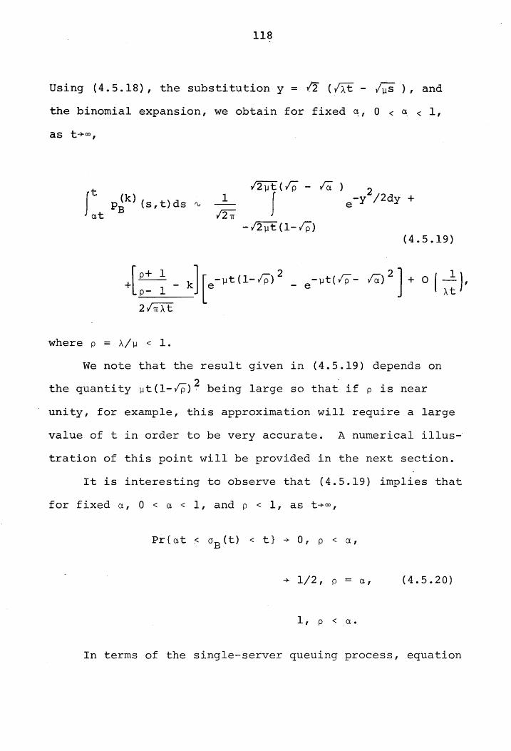
118
Using (4.5.18), the substitution y = (:2 (/it - I~s ), and
the binomial expansion, we obtain for fixed ~, 0 < ~ < 1,
as t+ oo ,
12~t(1P - 10.
Jt p~k) (s,t)ds ~ at
1
I2TI f ) 2 e-Y /2dy +
-/2~t (1-/P) (4.5.19)
+[ ~ _ k] [ e -]l t (1-1P) 2 _ e -)J t ( Ip" - raj 2 ] + 0 I A ~ ), 2/7fAt
where p = A/~ < 1.
We note that the result given in (4.5.19) depends on
the quantity ~t{l-IP)? being large so that if p is near
unity, for example, this approximation will require a large
value of t in order to be very accurate. A numerical il1us-
tration of this point will be provided in the next section.
It is interesting to observe that (4.5.19) implies that
for fixed a, 0 < a < 1, and p < 1, as t+ oo ,
Pr{at;< aBet) < t} + 0, p < a,
+ 1/2, p = a, (4.5.20)
I, p < a.
In terms of the single-server queuing process, equation

119
(4.5.40) implies that over a long period of time, the fraction
of time during which the server is busy is not likely to ex-
ceed p. This leaves the question as to the behavior of
Pr{at<oB(t)<t} when p = 1. It is not possible, of course,
for the server to be occupied for a fraction of time which
exceeds unity.
To answer this question we use equation (4.5.17) and
follow the same steps as in the non-s~~etric case. This
procedure leads to the result that for p = 1 and fixed a,
o < a < 1, then as t+oo ,
1211 t (1-1-;;)
It p~k) (s, t) ds ",.J?: J at TI 0
(4.5.21)
- 2 + k [1 - e- llt (l-la) 1 + 0 (-.!.), k =
lJ t 0,1,2, .•.
Evidently when p = 1, pr{at<oB(t)<t}+l as t+oo, i.e.,
over a long period of time, for fixed a, the server is likely
to be busy for a fraction of time which exceeds a. Therefore,
over a long period of time the server is likely to be busy
most of the time. It is possible, however, to approximate
pr{at<oB(t)<t} to a high degree of accuracy by using (4.5.21)
as will be illustrated in the next Section.
The limiting expression for pr{at<oB(t)<t} given by
(4.5.19) and (4.5.21) are similar to, but differ slightly
120
~
from, results obtainable from the work of Takacs [3.5]. In
the next Section, we shall compare Tak~cs' asymptotic results
with our own.
4,.6 Numerical Complements
The object of this Section is to illustrate the degree of
accuracy of the asymptotic formulae derived in Sections 4.3 -
4.5 and to compare these asymptotic approximations with those
suggested by the work of Takacs [35] wherever applicable. As
noted in Section 4.1, Takacs' work is based on the theory of
stable distributions discussed in Section 2.6. Although we have
used entirely different methods from those used by Takacs, our
limiting forms are similar to his, but there are slight differ-
ences which appear to affect the accuracy of the approximations
as we shall point out.
To this end we shall discuss in order the asymptotic re-
sults pertaining to the following:
(i) the strictly positive sojourn time for the unrestricted
random walk;
(ii) the zero and non-zero sojourn time for the unrestricted
walk; and
(iii) the busy time for the MIMll queuing process.
We assume throughout this Section that S(O) = O. All entries
in the Tables are believed to be correct to one unit of the
final decimal place.

121
We proceed now to discuss topics (i) - (iii) in turn.
i) The Strictly Positive Sojourn Time for the Unrestric
ted Random Walk with Negative Exponentially Distribu
ted Intervals Between Steps
Because of the difficulties of integrating the sojourn
density PB(s,t) given in (4.3.13), we shall focus attention
on the density function itself instead of on the distribution
function.
For the case A ~ ~, Takacs' results do not seem to apply_
The accuracy of our own approximation to PB(s,t) given in
(4.3.28) is illustrated in Table IV. It is assumed that
S(O) = o.
In Table IV we give the exact and approximate values of
PB(Ctt,t) for t = 50, 100, 150, 200; Ct = .2, .4, .6, .8; and
p = .6, .8, 1.2, 1.4. Under each value of t the exact and
approximate values are listed side by side for the different
values of p given in the first colu~~ and the values of Ct
given in the second column. We have assumed ~ = 1 in each
case.
From Table IV it is evident that equation (4.3.28) does
not provide a good approximation for the positive sojourn
density function. Nevertheless, it is clear that the rela
tive error in the approximation decreases as t increases.
Unfortunately, the convergence of the approximation to the

122
true value with increasing t is extremely slow. Equation
(4.3.28) was derived using only the leading terms of the
relevant asymptotic formulae, however, and greater accuracy
could be obtained by including higher order terms, which
would not be difficult.

TABLE IV
EXACT AND APPROXI~~TE VALUE~ OF PB(at,t)
t = 50 t = 100 t = 150 t = 200
0 a Exact AEErox. Exact AEErox. Exact AEErox. Exact ApErox.
0.6 0.2 0.012766 0.037189 0.003824 0.007910 0.001475 0.002590 0.000636 0.001012 0.6 0.4 0.003859 0.007910 0.000637 0.001012 0.000141 0.000199 0.000035 0.000046 0.6 0.6 0.001511 0.002590 0.000141 0.000199 0.000018 0.000023 0.000002 0.000003 0.6 0.8 0.000687 0.001012 0.000036 0.000046 0.000002 0.000003 0.000000 2x10- 7
0.8 0.2 0.018970 0.135421 0.009253 0.042829 0.005739 0.020854 0.003924 0.012116 0.8 0.4 0.010240 0.042829 0.004107 0.012116 0.002164 0.005277 0.001276 0.002742 0.8 0.6 0.006935 0.020854 0.002317 0.005277 0.001047 0.002056 0.000537 0.000956
I--' 0.8 0.8 0.005586 0.012116 0.001542 0.002742 0.000594 0.000956 0.000263 0.000397 tv
w 1.2 0.2 0.007719 0.017797 0.002331 0.004370 0.000979 0.001652 0.000472 0.000745 1.2 0.4 0.009185 0.030015 0.003283 0.008074 0.001585 0.003344 0.000867 0.001652 1.2 0.6 0.013035 0.060400 0.005471 0.017797 0.003019 0.008074 0.001863 0.004370 1.2 0.8 0.023163 0.187132 0.011552 0.060400 0.007346 0.030015 0.005152 0.017797
1.4 0.2 0.002344 0.003774 0.000251 0.000348 0.000037 0.000049 0.000004 0.000008 1.4 0.4 0.004138 0.008128 0.000668 0.001049 0.000147 0.000208 0.000034 0.000049 1.4 0.6 0.008555 0.020890 0.002064 0.003774 0.000660 0.001049 0.000236 0.000348 1.4 0.8 0.022675 0.082656 0.008363 0.020890 0.003933 0.008128 0.002053 0.003774

124
For the case, A =~, the asymptotic result suggested by
the work of Takacs and our approximation given in (4.3.28)
are the s~~e. Table V compares the exact and approximate
values of PB(s,t) assuming A = ~ = .1 and t = 100. As ap
plied-to a soccer game in which goals are scored at random
according to a Poisson process, these assumptions imply that
each team scores a goal on the average of one every ten min
utes during a 100 minute game. In Table V the values of s
are arranged in the left hand column while the exact and
approximate values are arranged in columns headed by the
words "exact lJ and "approximate", respectively.
We observe 'from Table V that away from the ends of the
range, [nls(t-s)]-l provides a good approximation for the
density PB(s,t). The approximate values do tend to over
estimate the true values, however, and for this reason we
expect that the arc sine approximation given in (4.3.30) will
have this same tendency to overestimate the distribution
function.

125
TABLE V
VALUES OF PB (5, t) FOR P = 1, t = 100
s Exact AEEroximate
b 0.1773 00
20 0.0763 0.0796
40 0.0633 0.0650
60 0.0633 0.0650
80 0.0763 0.0796
100 0.1773 00

126
We turn now to
ii) The Zero and Non-Zero Sojourn Distribution for the
unrestricted Random Walk with Negative Exponentially
Distributed Intervals Between Steps
Unfortunately, no meaningful approximations have been
derived for the case A ~ ~ as yet. Moreover, it is not clear
that the work of Takacs applies in this case since the dis-
tribution of TBA does not satisfy (2.6.6).
For the case A = ~, however, accurate asymptotic approx-
imations can be obtained. Our approximation for
Pr{at < aBet) < t} is given in equation (4.4.31). The cor
responding formula obtained from Takacs' results ([35], Theo-
rem 4, p. 284) is given by
t
J PB{s,t)ds at
12~t(1-a) 2 f2 J e-x /2dx = Pr{at < aBet) < t} ~VTI '
a (4.6.1)
which is the form of the stable distribution of order 1/2
given in (2.6.8). A comparison of (4.4.31) and (4.6.1) shows
that the two approximations are the same except for the dif-
ference in the upper limit of the integral. We point out
that (4.6.1) implies a dependence on a while our result given
in (4.4.31) depends upon fa. We are unable to explain this
difference at present. The practical effect of this differ-
ence is illustrated in Table VI below.

127
Table VI gives exact and approximate values of
Pr { at < cr B (t) '< t } for t = 10, 20, 3 0, and a = . 5 , • 6, • 7 ,
.8, .9. In this case aBet) represents the amount of time
during (O,t) that the random walk remains in the non-zero
state:' Under each value of t, the exact and approximate
values are given, with Takacs' approximation in the column
headed "Takacs" and the approximation based on (4.4.31)
given in the column headed "(4.4.31).n The corresponding
values of a are listed at the beginning of each row. Again
we have assumed S(O) = 0 and v = 1.
It is evident from Table VI that (4.4.31) is a uniformly
better approximation than Takacs' result given by (4.6.1).
Moreover, (4.4.31) has the desirable property of being very
accurate even for relatively small values of t.

TABLE VI
VALUES OF Pr{at < aBet) < t} FOR p = 1
t = 10 t = 20 t = 30
(l Exact (4.4.31) Takacs Exact (4.4.31) Takacs Exact (4.4 .. 31) Takacs
0.5 0.9784 0.9793 0.9984 0.9988 0.9989 0.9999 0.9999 0.9999 0.9999
0.6 0.9304 0.9323 0.9885 0.9899 0.9902 0.9996 0.9984 0.9984 0.9999
0.7 0.8224 0.8253 0.9422 0.9442 0.9450 0.9927 0.9810 0.9812 0.9989
0.8 0.6282 0.6313 0.7940 0.7949 0.7963 0.9263 0.8797 0.8805 0.9715 ...... tv 00
0.9 0.3436 0.3456 0.4729 0.4721 0.4734 0.6289 0.5610 0.5619 0.7266
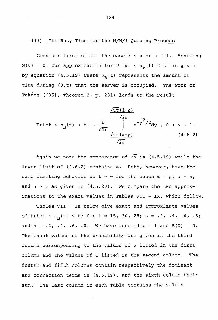
129
iii) The Busy Time for the MIMII Queuing Process
Consider first of all the case A < ~ or p < 1. Assuming
S(O) = 0, our approximation for,Pr{at < aBet) < t} is given
by equation (4.5.,,19) where aB (t) represents the amount of
time during (O,t) that the server is occupied. The work of
Takacs ([35], Theorem 2, p. 281) leads to the result
(~t(l-p)
Pr{o.t < aBet} < t} tV
12p 2/2 1
J 12"1f e-Y dy , a < 0. < 1.
(llt(o.-P) (4.6.2)
f2P
Again we note the appearance of {a in (4.5.l9) while the
lower limit of (4.6.2) contains 0.. Both, however, have the
same limiting behavior as t ~ 00 for the cases 0. < p, 0. = p,
and 0. > P as given in (4.5.20). We compare the two approx-
imations to the exact values in Tables VII - IX, which follow.
Tables VII - IX below give exact and approximate values
of Pr{o.t < aBet) < t} for t = 15, 20, 25; 0. = .2, .4, .6, .8;
and p = .2, .4, .6, .8. We have assumed ~ = 1 and S(O) = O.
The exact values of the probability are given in the third
column corresponding to the values of p listed in the first
column and the values of 0. listed in the second column. The
fourth and fifth columns contain respectively the dominant
and correction terms in (4.5.19), and the sixth column their
sum. The last column in each Table contains the values

130
calculated from Takacs' result given in (4.6.2).
The values given in Tables VII - IX illustrate that
for smaller values of p, (4.5.19) gives a better approxima
tion than that of Takacs. For values of p near unity, how-
ever, 'the accuracy of (4.5.19) diminishes as predicted be-
cause of the dependence on (1-0). For 0 near unity we no-
tice that as a increases, the correction term decreases the
accuracy of the approximation. The dominant term is then
seen to be of the same order of magnitude as the value of ~
Takacs' approximation.

131.
TABLE VII
VALUES OF Pr{<lt < 0B (t) < t} FOR t = 15
(4.5.19)
p (l Exact Dominant Cor. AEErox. Takacs
0.2 0.2 0.38095 0.49876 -0.12090 0.37786 0.49999 0.2 0.4 0.08861 0.15391 -0.07175 0.08206 0.11033 0.2 0.6 0.01404 0.03524 -0.02322 0.01202 0.00715 0.2 0.8 0.00140 0.00592 -0.00483 0.00109 0.00011
0.4 0.2 0.77107 0.82280 -0.06259 0.76021 0.80207 0.4 0.4 0.37446 0.47794 -0.11664 0.36130 0.49531 0.4 0.6 0.11794 0.19607 -0.08152 0.11455 0.18855 0.4 0.8 0.02216 0.05361 -0.03028 0.02333 0.03694
0.6 0.2 0.93764 0.85503 0.05008 0.90511 0.84270 0.6 0.4 0.67774 0.67338 -0.05112 0.62226 0.68160 0.6 0.6 0.33710 0.39150 -0.10029 0.29121 0.42135 0.6 0.8 0.10031 0.14731 -0.06385 0.08346 0.16110
0.8 0.2 0.99833 0.71129 0.29178 1.00300 0.69675 0.8 0.4 0.86781 0.64279 0.17913 0.82192 0.61951 0.8 0.6 0.58614 0.46264 0.01459 0.47723 0.45970 0.8 0.8 0.24870 0.21845 -0.05641 0.16204 0.22985

132
TABLE VIII
VALUES OF Pr{at. < 0B (t) < t} FOR t = 20
(4.5.19)
p a Exact Dominant Cor. ApErox. Takacs
0.2 0.2 0.39633 0.49976 -0.10555 0.39420 0.49999 0.2 0.4 0.07164 0.12044 -0.05302 0.06742 0.07864 0.2 0.6 0.00767 0.01896 -0.01216 0.00679 0.00233 0.2 0.8 0.00047 0.00210 -0.00170 0.00040 0.00001
0.4 0.2 0.82502 0.86926 -0.05077 0.81849 0.83999 0.4 0.4 0.38965 0.48995 -0.10855 0.38140 0.49865 0.4 0.6 0.10428 0.17428 -0.06987 0.10441 0.15730 0.4 0.8 0.01502 0.03072 -0.02168 0.01704 0.02140
0.6 0.2 0.96753 0.90380 0.03986 0.94366 0.89752 0.6 0.4 0.73254 0.73867 -0.04977 0.68890 0.74165 0.6 0.6 0.54301 0.58825 -0.08972 0.49852 0.44876 0.6 0.8 0.09378 0.14726 -0.06325 0.08401 0.15587
0.8 0.2 0.99548 0.74549 0.24813 0.99363 0.74330 0.8 0.4 0.91561 0.69906 0.17350 0.87257 0.68160 0.8 0.6 0.64320 0.52357 0.01580 0.53938 0.52049 0.8 0.8 0.26890 0.24783 -0.06341 0.18442 0.26024

133
TABLE IX
VALUES OF Pr{at < °B(t} < t} FOR t = 25
(4.5.19)
p a Exact Dominant Cor. Approx. Takacs
0.2 0.2 0.40694 0.49953 -0.09457 0.40496 0.50000 0.2 0.4 0.05793 0.09507 ':"0.04007 0.05500 0.05692 0.2 0.6 0.00422 0.01026 -0.00644 0.00382 0.00078 0.2 0.8 0.00016 0.00073 -0.00059 0.00014 1x10- 6
0.4 0.2 0.86374 0.90020 -0.04058 0.85962 0.86782 0.4 0.4 0.40036 0.49532 -0.10052 0.39480 0.49960 0.4 0.6 0.09185 0.15275 -0.05924 0.09351 0.13137 0.4 0.8 0.01018 0.02730 -0.00498 0.00301 0.00219
0.6 0.2 0.98270 0.93420 0.03090 0.96510 0.93211 0.6 0.4 0.77451 0.78708 -0.04700 0.74008 0.78540 0.6 0.6 0.36764 0.44451 -0.10477 0.33974 0.46605 0.6 0.8 0.08680 0.14291 -0.06083 0.08208 0.16671
0.8 0.2 0.99849 0.77153 0.21291 0.98444 0.77654 0.8 0.4 0.94504 0.74033 0.16377 0.90410 0 .. 72847 0.8 0.6 0.68828 0.57391 0.01658 0.59049 0.57080 0.8 0.8 0.28444 0.27232 -0.06902 0.20330 0.28540

134
For the case A = ]..1, sometimes referred to as the "heavy
traffic" situation, our result is given in (4.5.21). Takacs'
analysis ([35], Theorem 4, p. 284) gives a similar result,
namely,
(4.6.3)
Again both (4.5.21) and (4.6.3) are given in terms of
the stable distribution of index 1/2 while (4.5.21) depends
on ~ and (4.6.3) on a. As an approximation (4.5.21) seems
to be preferable to (4.6.3) as illustrated in Table X below.
Table X gives exact and approximate values of
Pr{a.t < 0B (t) < t} for t = 15, 20, 25, 30; a = .5, .6, .7 ,
.8, .9. It has been assumed that S (0) = 0 and A = ]..1 = 1.
Under each value of t, the second column contains the correct
value corresponding to the value of a given in the first
column. The third and fourth columns under each value of t
are the values of equations (4.5.21) and (4.6.3), respec
tively, and are labeled "(4.5.21)" and "Takacs".

135
TABLE X
VALUES OF Pr{at < 0B (t) < t} FOR A = l.l = 1
t = t = 20
(4.5.21) Takacs (4.5.21) ~
a Exact Exact Takacs
0.5 0.8892 0.8913 0.8290 0.9348 0.9360 0.8861
0.6 0.7805 0.7830 0.7266 0.8443 0.8460 0.7940
0.7 0.6266 0.6290 0.5886 0.6966 0.6984 0.6572
0.8 0.4350 0.4369 0.4161 0.4941 0.4956 0.4729
0.9 0.2203 0.2213 0.2158 0.2536 0.2544 0.2481
t = 25 t = 30
a Exact (4.5.21) ....
Takacs Exact (4.5.21) Takacs
0.5 0.9609 0.9616 0.9229 0.9763 0.9767 0.9471
0.6 0.8878 0.8890 0.8427 0.9183 0.9191 0.8786
0.7 0.7504 0.7519 0.7111 0.7930 0.7942 0.7547
0.8 0.5433 0.5446 0.5204 0.5854 0.5865 0.5614
0.9 0.2825 0.2832 0.2763 0.3083 0.3089 0.3014

136.
4.7 The Three-State Sojourn Time Problem
In this Section we consider the more difficult sojourn
time problem in which it is assumed that the particle may be
in anyone of three possible states at a given time t. We
assume that S(O) = 0 and that a transition to state A has
occurred just prior to t = O. The alternative states are
denoted by Bl , B2 • We define get) by the equation
g(t)dt = Pr{t < min[TAB ,TAB] < t + dt}, 1 2
(4.7.1)
and hl(t), h 2 (t) are similarly defined in a manner consistent
with the definitions of Section 4.2.
We shall assume that from states B1 , B2 the random walk
can only make a transition to state A. We shall also assume
that, given that a transition from A to Bl or B2 occurs, the
probability of transition to Bl (or B2 ) is a constant, i.e.
independent of time. Because of this assumption we define
and
P2 = Pr{S (t+dt) E B21 S (t) E Ai S (t+dt) E (B lUB 2)}. (4.7.3)
Using these assumptions we proceed to derive an expres-
sion for p(r,sit) which is defined by
137
p(r,s,t)drds = pr{r<oA(t)<r+dr; s<oB (t)<s+dsIS(O) = ol, 1
o < r, s < t. (4.7.4)
The derivation of. p(r,s,t) follows the same general pattern
as that given in Section 4.2 for the two-state sojourn density
function. As mentioned previously, Good [23] has obtained
the counterpart of p{r,s,t) for n states and expressed it in
terms of a multiple contour integral. Good has obtained his
results, however, under assumptions which differ slightly
from ours. In Good's analysis he has assumed that the infin-
itesimal transition probabilities, Pr{S(t+dt) E A\S(t) E B.} ~
and Pr{S(t+dt) E B. IS(t)} E A, are constant, i = 1, 2. In 1
this Section we shall use a direct approach to derive p(r,s,t)
which is instructive and leads to an explicit result.
The general expression obtained will then be applied to
the unrestricted random walk in which it is assumed that the
particle is in state A at time t if Set) = 0, in state Bl if
Set) > 0, and in state B2 if Set) < o.
Both the general result and the application given in this
Section have not been discussed in the literature previously.
At a given time t the particle must be in one of the
three states A, BI
, or B2 and there is no other possibility.
We begin our analysis by defining Umn(r,s,t)drds as the proba
bility that
(i) Set) E A~
l3~
(ii) 0A{t) is composed of m disjoint intervals of time
and r < 0A(t) < r + dri and
(iii) 0B (t) is composed of n disjoint intervals of time 1
and s < 0B (t) < S + ds. 1
Obviously the definition of umn(r,s,t) implies that
t-r-s-ds-dr < 0B (t) < t-r-s. 2
We define v (r,s,t) and mn
wmn{r,s,t) in the same manner except for the sUbstitution of
Set) £ Bl and Set) £ B2 in (i) above, respectively.
For convenience of notation we shall let umn(r,O,t)dr
be defined according to (i) - (iii) above with the exception
that in (iii) we replace s < 0B (t) < S + ds by 0B (t) = O. I I
Similarly, the probability u {r,t-r,t)dr is also defined mn
according to (i) - (iii) with the exception that in (iii) the
phrase, t-r-dr < 0B (t) < t - r, is sUbstituted for 1
s < 0B (t) < S + ds. An analogous convention will be used 1
to define v (r,O,t)dr, v (r,t-r,t)dr, w (r,O,t)dr, and mn mn mn
wmn(r,t-r,t)dr. Although not usually done, it seems logical
and most convenient to extend the usual probability density
function notation to apply to the mixed probability and proba-
bility density function in this manner.
We note that since S(O) £ A, we have
= 0 i s < 0B (t) < S + ds} = 0, 0 < s < t, (4. 7 .5) 1

l3~
and since 0A(t) = t implies that no transition from state A
to Bl or B2 occurs during the interval (O,t), we have
pr{oA(t) = t} = 1 - G(t). (4.7.6)
We first derive ~n(r,s,t) and then indicate the modifi
cation necessary to obtain expressions for v (r,s,t) and mn
w (r,s,t). Consider then mn
Case I. 0 < r < t, s = 0
The assumption s = 0 implies that no passage to state Bl
occurs during (O,t) and consequently u (r,O,t) is zero if mn
n F O. Since 0 < r < t, the particle must make a passage to
state B2 at some time x followed by an interval of time of
length y, 0 < y ~ t-r, during which the particle remains in
state B2
• In order to have Set) E A, the particle must return
to state A at some time and hence GA(t) must be composed of
at least two disjoint intervals of time, i.e. m z 2. If
m = 2, we see from the foregoing considerations that
(4.7.7)
= P2h 2 (t-r) [G (r) -G (2) (r)] .
For m Z 2, it is evident that after the initial return to
state A from state B2
, the process begins again with the
140.
remaining portion of the interval (O,t) consisting of m - 1
disjoint intervals during which the particle remains in state
A and no time spent in state Bl - Consequently, we can write
Jr ft-r
umO(r,O,t} = 0 g{x)dx ° P2h 2(y)um_1 ,0(r-x,0,t-y-x)dy,
m = 3, 4, _ •• _ (4.7.8)
By application of mathematical induction to (4.7.7) and
(4.7.8),we find that
umO
(r, 0, t) = pJm-l) (t-r) [G (m-l) (r) - G (m) (r) ] ,
m = 2, 3, •... (4.7.9)
We turn then to
Case II. ° < r < t, s = t - r
Because of the assumption that s = t - r, Case II cor-
responds exactly to Case I except that now aB (t) = 0 rather 2
than aB (t) = o. Since Set) € A, aB (t) = ° implies that 1 2
m = n+1, n = 1,2,3, ...• By argument analogous to that used
for Case I,it is evident that
u21 (r,t-r,t) = J: g(x)P1h1(t-r) [l-G(r-x)]dx
(4.7.10)
= Plh(t-r) [G{r) -G (2) (r)]
141
and
x u (r-x t-r-y t-x-y)dy m-1,m-2 " ,
m = 3, 4, 5, .... (4.7.11)
Again by mathematical induction we find that
um
,m-1 (r, t-r, t) = pim- 1 ) hI (m-l) (t-r) [G (m-l) (r) -G (m) (r) ] ,
m = 2, 3, ..•• (4.7.12)
Finally, we consider
Case III. 0 < r < t, 0 < S < t - r
In this case we have 0 < GA(t) , GB (t), GB (t) < t, i.e. I 2
the particle spends some time in all three states. Therefore
we conclude that n > 1 and m > n + 2.
Consider first of all u 3l (r,s,t)drds. In this case aBet) 1
and aB
(t) each consist of one interval of time and satisfy 2
the inequalities s < GB
(t) < S + ds and t-s-r-ds-dr < G (t)< 1 B2
t-s-r, respectively. There are two possibilities: either
state BI is visited first or state B2 is visited first.
142
Consequently, we write
(4.7.13)
For higher values of m we use the fact that the process renews
itself whenever a transition to state A occurs to write
J
r Jt-r-s + 0 g(x)dx 0 P2h 2(y)um_l ,1(r-x,s,t-x-y)dy,
m = 4, 5, •••• (4.7.14)
substituting (4.7.9) in (4.7.14) and applying induction, we
obtain
m = 3, 4, (4.7.15)
In a similar manner by induction on n and using the relation

143
(4.7.16)
we find that
x [G(m-1) (r)-G(m) (r)], m > n + 2, n = 1,2,3, ••. ,
o < r, s < t. (4.7.17)
Since the arguments used to obtain expressions for
Vmn(r,s,t) and wmn(r,s/t) are essentially the same as those
used to obtain u (r,s,t), with obvious modification, we ron
simply summarize these results as follo,\is:
v (r,O,t) = 0, m > n, n = 0,1,2, ... ; mn
v (r, t-r, t) = g (m) (r) pml [H (m-I) (t-r) -H (m) (t-r) ] ; m,m
m ~ n+l, n = 1,2, .•. , 0 < r, s < t.
w (r,t-r,t) = 0, m, n - 1, 2, mn ••• I
(4.7.18)
(4.7.19)
(4.7.20)
(4.7.21)

144
Wmo
(r, 0, t) = p~g (m) (r) [H~m-I) (t-r) -HJm) (t-r) ], m = I, 2, ••• ;
(4.7.22)
and
_(m-I) (m) ( ) n m-n wmn(r,s,t) - n g r P1P2 x (4.7.23)
x [HJm-n-1) (t-r-s) _H~m-n) (t-r-s) ] hin ) (s) ,
m ~ n+1, n = 1,2, .•. , a < r, s < t.
Combining the above we have
<Xl <Xl
p(r,s,t) = L L u (r,s,t) + n=l m=n+2 mn
(4.7 .. 24) 00 <Xl
+ I 2 [v (r,s,t) + wmn(r,s,t)], 0 < r, s < ti n=l m=n+1 mn
Pr{ 0A (t) = t} = 1 - G(t); (4.7.25)
00
pr{r<oA(t) <r+dr; °B (t) = o} = I umO(r,O,t)dr + 1 m=2
(4.7.26) 00
+ 2 wmO(r,O,t)dr, 0 < r < ti m=l
and
00
Pr{r<oA(t) <r+dr; °B (t) = O} = I u l(r,t-r,t)dr + 2 m=2 m,m-
00 (4.7.27)
+ I v {r,t-r,t)dr, 0 < r < t. m=l m/m

145
This completes the derivation of the general sojourn
density function for the three-state sojourn time problem.
As a partial check on our analysis we should find that
fto fto-.r. Jt p(r,s,t}dsdr + 0 pr{r<oA(t)<r+dr; oBI (t) = O}dr +
(4.7.28)
+ fto pr{r<oA(t)<r+dr; 0B (t) = 2
O}dr + pr{oA(t) = t}= 1.
Taking Laplace transforms with respect to the variable t, we
find that
L[J
t
o Jto-r ] p(r,s,t)dsdr = Plg*(z)G~(z)hi(z) x
x[r1-p g*(z)h*(z») [l-p !*(Z)h*(Z)-P g*(z)h*(z)] 2 2 112 2
(4.7.29)
L[J: Pr{r<aA(t) <r+dr; 0B (t) O}dr] P2g* (z) [l-g* (z)h2 (z)]
= = z[1-P2g*(Z)hi(z)] 1
(4.7.30)
L[J: Pr{r<aA(t) <r+dr; 0B (t) O}dr] Plg*(z) [l-g*(z)h!(z)]
= = z[l-Plg*(z)h!(z)] 2
(4.7.31)

and
where
and
L[pr{oA{t)
g* (z)
146
= t}] --[l-g*(z)]
z
00
= J -zt e g(t)dt, ,0
-zt e h. (t)dt, ~
i = 1, 2,
G*(z) = 1 [l-g*(z}]. c z
(4.7.32)
(4.7.33)
(4.7.34)
(4.7.35)
Equation (4.7.29) follows from (4.7.24) with the aid of
the identity
00
I (m+nn) xm = (l_x)-(n+l), m=O Ix\ < 1.
The derivations of (4.7.30) - (4.7.32) follow in a straight-
forward manner from (4.7.25) - (4.7.27).
Adding (4.7.29) - (4.7.32) yields a sum equal to liz
which implies that (4.7.28) holds.
We now apply the results given in (4.7.24) - (4.7.27)
to the unrestricted random walk in which it is assumed that
steps of +1 and -1 occur according to a Poisson stream with
parameters A, ~, respectively. We say that the particle is

147
in state A at time t if Set) = 0, in state Bl if Set) > 0
and in state B2 if Set) < O. In order to obtain an expres
sion for p(r,s,t), we proceed to determine the quantities
contained in equations (4.7.24) - (4.7.27). A transition
from state A to states Bl or B2 takes place if a positive or
negative step occurs. Therefore, we have
= Pr{S(t+dt) > Ols(t) = 0; S(t+dt) ~ O}
= Pr{positive step occurs during (t,t+dt) a step
occurs during (t,t+dt)}
(4.7.36) Adt A = = (A+~)dt A+~·
Similarly,
(4.7.37)
It is evident that pr{t<min(lAB ,lAB] < t + dt} is equal to 1 2
the probability that a positive or negative step occurs
during (t,t+dt), and hence,
(4.7.38)
Also, pr{t<oB A<t+dt} is the probability that a first passage 1
to zero occurs during (t,t+dt) given that a passage from
148
o to +1 occurred at time t = O. Hence,
Similarly,
h 2 (t) = f01{t). (4.7.4D)
We can now summarize the results corresponding to equations
(4.7.24) - (4.7.27) as follows:
(4.7.41)
= D} -_ e-(A+~)r ~ [~mr)!m fo(ml ) (t-r) + pr{r<oA(t) <r+dr; 0B (t) L 1 m=l·
(4.7.42)
+ ~(~r)m-l[F (t-r)-F (t-r)]]dr i (m-l) ! D,m D,m-1
I [<xr)mfim) (t-r) + m=l m! 0
(4.7.43)
+ A(Ar) [Fro O(t-r)-Fm
_l
O(t-r)] dri m-I ]
(m-I) !' ,
and
p{r,s,t)
m-I ~ (~r) (n)
f (s) [F (t-r-s) -F (t-r-s)] + 10 O,m O,m-l (m-I) ! n!

149
A(Ar)n-l (~r)m () ] + fo~ (t-r-s) [Fn,O(S)-Fn_l,O(s)] ,
(n-l)!· m!
o < r, S < t. (4.7.44)
1\:dopting the Laplace transform technique used in the
previous Sections in this Chapter, we obtain after tedious
calculation the following explicit expressions:
( )
1/2 + A]l~t-r) Il[~(r)l}dr +
-Ar + (A -~ ) e J [ II t , A (t - r) ] dr i ( 4 . 7 • 46)
where
~(r) = 2/Allt(t-r) (4.7.47)
and

150.
p(r,s,t) = e-(A+1-1}tM(r,S)N{r,s,t) +
where
and
-(A+ll)S + e . M(r,S)pr{r<O"A (t-s) <r+dr; O"B (t-s) = O} + 2
+ e-(A+ll) (t-r-s)pr{r<O"A(r+s) <r+dr; O"B (r+s) = O} x
2
x N(r,s,t), o < r, s < t, (4.7.48)
(4.7.49)
N(r,s,t) = ( All )1/2 rI1[!2(r,s,t)]' (4.7.50)
(t-s) (t-s-r)
~l(r,s) = 2~s(r+s) ~2(r,s,t) = 2/All(t-S) (t-s-r)
(4.7.51)
We note that p(r,s,t) is the product of functions of arguments
r(r+s) and (t-r) (t-r-s) which is analogous to the two-state
result.
As a partial check on our analysis we ,should find that
151.
pr{r<oA(t) <r+dr; 0B (t) = O} + pr{r<oA(t) <r+dr; 0B (t) = O} + 1 2
+ J:-r p(r,s,t)ds = PB(t-r,t) (4.7.52)
where PB(s,t) is the non-zero sojourn density given by equa
tion (4.4.14). With the aid of [17], Vol. I, we find, after
much algebraic manipulation, that
1 J zt-Zr Ar¢10{z) Pr{r<oA(t) <r+dr; 0B (t) = O}= e {e -1 +
1 2ni C
(4.7.53)
Ar¢10(z) +. A~lO (z) e }dzdr;
1 J zt-Zr ur ¢Ol(z) pr{r<oA(t) <r+dr; 0B (t) = O}= e {e -1 +
2 2ni C
and
Jt-r p(r,s,t)ds = O·
(4.7.54)
Ur ¢Ol(z) + U~Ol(z)e }dzdri
1 J zt-Zr Ar¢10(z) ur¢Ol{z) e { [e -1] [e -1] +
2ni C
(4.7.55)

152
where Z = A + II + z, C is the usual Laplace inversion contour
and ~ (z) and ~ (z) are defined in (3.1.2). Adding, we ron ron
obtain, with the aid of (3.2.13) and (3.2.18), the result
1 2ni
(4.7.56)
where R2 = z2 - 4All. Upon inversion using [17], ·Vo1. I, (36),
(37), p. 249, (4. 7 . 56) becomes
pr{r<oA(t) <r+dr}
t
+ (A+~)Io[i3(r)l]dr + (A_~)2 Jre-(A+~)X x
(4.7.57)
where
(4.7.58)
Then using (2_4.11), it is not difficult to show that
(4.7.59)
153
Upon combining (4.7.57) and (4.7.59), we see that (4.7.57)
agrees with (4.4.14).
No asymptotic results have been obtained so far.

CHAPTER V
CONNECTION OF THE RESULTS FOR THE UNRESTRICTED
RANDOM WALK IN DISCRETE TI~ffi AND THE
WORK OF E. SPARRE ANDERSEN WITH THE
UNRESTRICTED RANDOM WALK IN CONTINUOUS TIME
5.1 Introduction
By discrete-time random walk we mean the random walk in
which the particle moves to the right or left in steps of
unit length at epochs which may be numbered consecutively
1, 2, 3, .•• , but where we are unconcerned with the amount
of time between these epochs. The work contained in [18],
Chapter III, dealing with the discrete-time random walk,
demonstrates a connection between our results and those for
the unrestricted random walk in discrete time. It is possi
ble to derive at least some of the results for the unrestrict
ed random walk in continuous time from the discrete-time re
sults. These derivations utilize probabilities conditioned
on the number of steps during a given time t and the proba
bility that a certain number of steps take place in time t.
This procedure will be used in Section 2 to show how first
passage time densities and state probabilities for the con
tinuous-time random walk can be obtained from the correspond
ing results in discrete time. In Section 3, we shall show
154

155
the connection of several of our results with analogous re-
suIts for discrete time discovered by E. Sparre Andersen.
The connection does not, at first sight, seem obvious.
We summarize now the basic results for discrete-time
random walks needed in Section 2 and 3. For a detailed dis-
cussion, see [18]. It is assumed that the particle moves on-
ly at fixed epochs numbered 1, 2, 3, .•.. We let X. = + 1 1
according to whether or not the ith step is positive or neg-
ative, i = 1, 2, 3, .... It is assumed that
Pr{X. = +1} = Pi Pr{X. = -l} = qi i=1,2,3, ... , (5.1.1) 1 1
where
p + q = 1 , 0 < p < 1. (5.1.2)
th The position of the particle at the end of the r step is
then equal to
Sr = Xl + X2 + ... + Xr ' r=1,2,3, ... , (5.1.3)
assuming that
(5.1.4)
where So denotes the position of the particle initially.
The state probabilities are given by the equations
r+n r-n
Pn(r) = pr{Sr = n} = (r;~)p--2- q--2- (5.1.5)

156
and
r-n r+n
p (r) = Pr{S = -n} -n r = (r;n)p-2- q 2- ,n,:r,
(5.1.6)
r=O ,1,2, •.. ,
where r, n are both odd or both even.
The probability of first passage from 0 to n at time
2r-n is given by the equation
n (2r-n) r f (2r-n) = -- p On 2r-n r r-n
q , r=n,n+l, ... ,
n=1,2, ...•
(5.1.7)
We now turn to the application of these results to the
unrestricted random walk in continuous time with negative
exponentially distributed intervals between steps.
5.2 Extension of Discrete-Time Results to continuous
Time for the Random Walk with Negative Exponentially
Distributed Intervals Between Steps
We assume, as before, that positive and negative steps
occur according to two independent Poisson streams with pa-
rameters A and ~, respectively. The probability that a pos-
itive step occurs during the small interval (t,t+dt) is then
Adt and, similarly, the probability that a negative step
occu~s during (t,t+dt) is equal to ~dt. Consequently, the
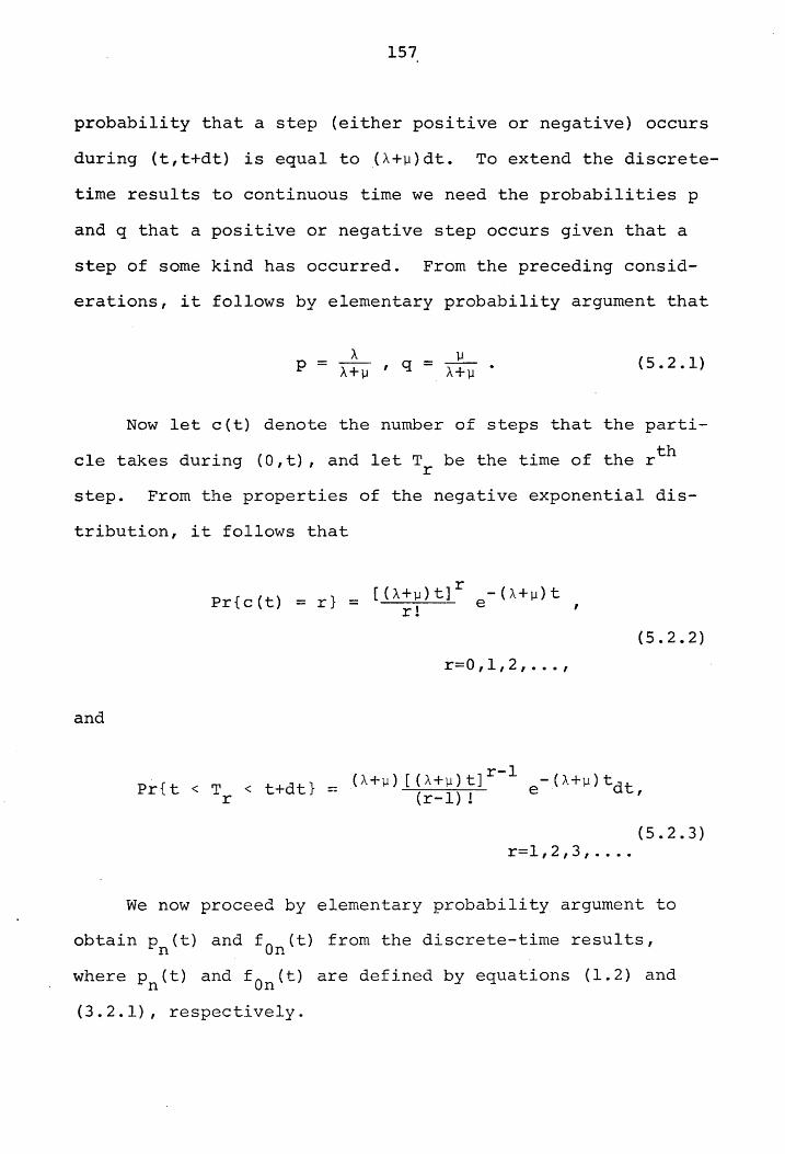
157
probability that a step (either positive or negative) occurs
during (t,t+dt) is equal to (A+~)dt. To extend the discrete-
time results to continuous time we need the probabilities p
and q that a positive or negative step occurs given that a
step of some kind has occurred. From the preceding consid-
erations, it follows by elementary probability argument that
A p = ~ , q = II
A+~ • (5.2.1)
Now let c(t) denote the number of steps that the parti
cle takes during (O,t), and let T be the time of the rth r
step. From the properties of the negative exponential dis-
tribution, it follows that
Pr{c(t) = = [(A+ll)t]r -(A+~)t r} ---r-!-- e ,
(5.2.2)
r=O ,1,2, •.• ,
and
. = (A+ll) [(A+ll)t]r-l e-.(A+~)tdt, Pr{t < T < t+dt} -r (r-l) !
(5.2.3) r=1,2,3, ....
We now proceed by elementary probability argument to
obtain p (t) and fO (t) from the discrete-time results, n n
where p (t) and fa (t) are defined by equations (1.2) and n n
(3.2.l), respectively.

158.
First of all, from (5.1.5) and (5.2.2) we find that
p (t) = Pr{S(t) = n 1 S(O} = O} n
00
= I pr{Sr = n}Pr{c(t) = r} r=n
r+n r-n 00 __
t ( r) 2 q--2--[(A+~)t]r e-(A+~)t = r;n r;n P r!
(5.2.4)
where it is understood that the terms in (5.2.4) vanish if
r+n is odd. By use of (5.2.1) and upon simplification,
(5.2.4) becomes
p (t) n = (~ln/2 e-(A+~)t r
r=O
where
p = f.l
(Af.lt2)r+n/2 (r+n) !r!
(5.2.5)
(5.2.6)
The latter part of (5.2.5) follows directly from (2.3.1).
We note that (5.2.5) agrees with equation (2.3.12).
Similarly, by use of equation (5.1.7) and (5.2.3) I it
follows that

159
L fOn(m)Pr{t < Tm < t+dt} m=n
00
= e-(A+~)t n L m=O
An+m~mt2m+n-l
(m+n) 1m! (5.2.7)
-(A+~)t n/2 .;--= e np I (2t A~)/t , n=1,2, ••.• n .
Equations (5.2.5) and (5.2.7) are given in [19] where
these same methods were used to obtain them. It is possible
that other results for the continuous-time case can be de-
rived using discrete-time results. It seems simpler, how-
ever, to follow the methods used in Chapters III and IV.
5.3 Connection with the Work of E. Sparre Andersen
E. Sparre Andersen's fundamental research [1] and [2]
concerning the fluctuations of sums of random variables is
summari , perhaps more accessibly, in [19] and [33]. We
concentrate attention on four of Andersen's results which
bear a striking resemblance to our results for continuous
time:
i) Consider a discrete-time unrestricted random walk
for which the size of each step X. has a common 1
distribution and let So = 0, Sl' 52' 8 3 , ... , 8n be
~he sequence first n par~ial sums of the x .. If 1
N is the number of positive terms among n
81
, 82
, ... , 5n
, then

160.
ii) Let v be the number of steps (or time) required to
reach the first maximal term Sv among SI' 52' ••. , 5n
so that Sv>O, 5 v>Sl' ••• , Sv>Sv-l' Sv~Sv+l' Sv~Sv+2'
S > S +3' .•. , S > S. Then v- v v- n
Pr{v = k} = Pr{N n
= k} •
iii) For fixed a, 0 < a < 1, as n + 00,
2 Pr{N < na} + -arc sin I~ . n 'IT
(5.3.2)
(5.3.3)
iv) For a walk with steps of ±1, let Tn be the probabil
th ity of first passage from 0 to +1 at the n step
(time n). Moreover, let T(S) be the generating
function of T , viz., n
T(S) = L n=l
Then
-1 log[l - T(S)] = 00 n L ~
n=l n
n s T n
Pr{S > O} • n
(5.3.4)
Equation (5e3.1) corresponds to PB{s,t) for the posi
tive sojourn time defined in (4.2.1) and given by (4.3.13),
because F01 (t-S) is the probability that a particle, begin
ning its walk at the origin, does not pass into the positive

161
state throughout the time interval (O,t-s). In other words,
FOl(t-s) = pr{oB(t-s) = 0 I S(O) = O} , (5.3.5)
where 0B(t) denotes the amount of time during (O,t) that the
particle spends in state B, the positive state. Similarly,
FlO(S) = pr{oB(s) = s I S(O) = l} • (5.3.6)
The factor A in (4.3.13) can be explained on the grounds
that equation (4.3.13) was derived assuming S(O) = 0 so that
Ads is the probability of its immediate passage into the
strictly positive state.
The result stated in paragraph (ii) is simply the ana-
logue of the result
m(s,t) = PB(s,t) , (5.3.7)
where m(s,t) is defined by (3.5.5) and given in (3.5.9).
Equation (5.3.3) corresponds directly to equation
(4.3.30), which expresses the asymptotic behavior of the ran-
dom variable 0B(t)/t, i.e., the distribution of 0B(t)/t and
the distribution of N In have the saIne asymptotic behavior. n
Concerning (iv) we note from (5.2.5) and (5.2.7) that
.!. fO (t) = n n (5.3.8)
and hence,
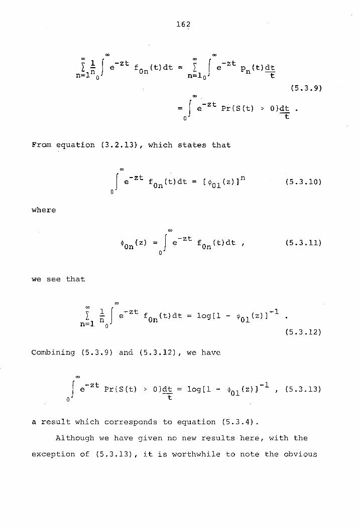
162
00
00 J L 1 n=ln
O
-zt e fOn(t)dt = I f e-
zt p (t)dt
n=lo n ~
(5.3.9)
: f e-zt Pr{S(t) > O}dt • o ~
From equation (3 • 2 .. 13) , which states that
00
J e-zt
fOn(t)dt n (5.3.10) = [ <PO 1 (z) ]
0
where
00
<POn (z) J -zt fOn(t)dt , (5.3.11) = e
we see that
00
~ J a
I n=l
00
-zt e fOn(t)dt
-1 = 10g[l - ¢Ol(z)]
Combining (5.3.9) and (5.3.12), we have
00
(5.3.12)
J e -zt -1 P r { S (t) > O} d t = 10g [1 - ¢ 0 1 (z) ] ,( 5 .. 3 . 13 )
a t
a result which corresponds to equation (5.3.4).
Although we have given no new results here, with the
exception of (5. 3 . 13), it is worthwhile -to note the obvious

163
comparisons between our work and that of E. Sparre Andersen.
An elegant exposition of the results given in this Section
is included in an unpublished paper by B. W. Conolly [11].

CHAPTER VI
SOME GENERAL RESULTS FOR THE UNRESTRICTED RANDOM WALK
AND THE SINGLE-SERVER QUEUING PROCESS
6.1 Introduction
Until now we have considered only cases in which posi
tive and negative steps occur according to a Poisson stream.
In this Chapter we shall summarize certain results pertain
ing to the unrestricted and queuing random walks under more
general assumptions. Since most of our work is concerned
with the unrestricted random walk, we shall postpone a.ny
further remarks about the queuing process until Section 6.5.
Therefore, the reader may assume that, with the exception
of Section 6.5, the discussion in this Chapter applies only
to the unrestricted random walk.
The extension that will be made in Sections 6.2 - 6.4
is a natural consequence of removing the barrier at zero in
the queuing random walk. We shall be concerned with the
development of results in the unrestricted case which cor
respond to the GI/M/I and MIGII queuing systems described
in Chapter I.
First of all, let A(t) denote the distribution function
of the length of time between positive steps, and let aCt)
denote its probability density function. Similarly, denote
164

165.
by B(t) the distribution function of the time between nega-
tive steps with its corresponding probability density func-
tion denoted by bet). We define A (t) and B (t) by the c c
equations
and
A (t) = 1 - A{t) c
B (t) = 1 - B{t) • c
(6.1.1)
(6.1.2)
We continue to assume throughout Sections 6.2 - 6.4
that positive and negative steps occur independently of each
other. As a result of this assumption, we have, for the
unrestricted random walk,
Pn(t} = Pr{S(t) = n I S(O) = O}
(6.1.3) 00
= I {A (m+n) (t) - A (m+n+l) (t) } {B (m) (t) - B (m+l) (t)} , m=O
and
P (t) = Pr{S(t) = -n I S(O) = O} -n
= 00
I {A (m) (t) - A (m+l) (t) } {B (m+n) (t) - B (m+n+l) (t) } m=O
n = 0,1,2, ••• , (6.1.4)
where
,

and
166
t
A(m) (t) = J A(m-1) (sla(t-s)ds , m = 1,2,3, ••• ,
o
The function B(m) (t) is similarly defined.
Borrowing from the notation of queuing theory, we shall
denote by lloo2/M/G" the doubly-infinite or unrestricted ran-
dom walk for which
-At aCt) = Ae (6.1.5)
and bet) is general. Similarly, we let fl oo 2/GI/M u designate
the unrestricted random walk for which
b (t)
and aCt) is general.
-lIt = lle ,.... (6.1.6)
Under the more general assumptions of oo2/M/G and
oo2/G1/ M, we lose the convenient Markov property associated
with the Poisson process. For example, in the oo2/GI/M walk,
if one considers an arbitrary point to in time, the prob
ability that the next positive step occurs at time to + T
depends on the length of time which has elapsed since the
previous positive step. Consequently, the probability that
the next positive step occurs at time to + T is independent
of the time elapsed since the previous positive step only

167.
if that step has just occurred, i.e., it occurred during
the interval (to-dt,tO). For this reason we say that the
process renews itself at the time of a positive step, and
the instants at which positive steps occur we call renewal
epochs. 2 Analogous considerations apply to the walk 00 /M/G.
To avoid difficulties in analysis, we shall always assume
that time t = a is a renewal epoch. The fact that the proc-
ess begins again, so to speak, at a renewal epoch will be
very important in the analysis to follow.
In Sections 6.2 and 6.3 we shall discuss first-passage
times and the time of occurrence and magnitude of the first
maximum for the oo2/M/G random walk. The corresponding top
ics for oo2/GI/M are discussed in Section 6.4. As mentioned
previously, we shall discuss the sojourn time problems for
the MIGII and GI/M/l queuing processes in Section 6.5. AI-
though the techniques used are not new, the results given
here have apparently not been published before.
6.2 First-Passage Time from m to n for oo2/M/G
As in Chapter III we define f (t) by the equation mn
fmn(t)dt = Pr{S(t+dt) = n S (x) :f n , 0 < x < tiS (0) = m}
(6.2.1)
given that t = 0 is a renewal epoch, i.e., a transition from
state m + 1 to state m takes place. Since we shall discuss
only the unrestricted random walk in this Section, it suffices

168
to consider the case where S(O) = 0 and a transition from
+1 to 0 occurs at t = O.
We shall derive a system of equations which relates the
probabilities fOn(t)dt, n = 1,2, ••. , by using the fact that
= fa (t), m = n+ 1, n+2 , •.. , ,m-n (6.2.2)
and analyzing the possible behavior of the particle until
the time when the first negative step occurs, that is, until
the first renewal epoch.
During the interval (O,t) either no negative step occurs
or at least one negative step occurs. If no negative step
occurs during (O,t), then the nth positive step must occur
at time t in order that a first passage to n take place at
time t. On the other hand, suppose the first negative step
occurs at time s, 0 < s < t, and j positive steps occur dur-
ing (D,s), 0 < j < n. Since s is a renewal epoch, a first
passage to n takes place at time t only if a first passage
from j - I to n occurs at the end of a further time t - s.
The foregoing considerations are summarized by the equation
= A(At)n-l e- At B (t) + (n-l) ! c
t
J -AS + e
a
(6.2.3)
n-l (AS)r b(s) I r! fO,n+l_r(t-s)ds.
r=O
Now define the generating function F(x,t) and its Laplace
transform ¢(x,z) by

169
Q()
\' xn () F(x,t) = L fOn t n=l
(6.2.4)
and Q()
J e-zt
~(x,z) = F(x,t)dt • o
(6.2.5)
From (6.2.3) it follows that
F (x, t)
t (6.2.6)
+ J b(s)e-\s(l-X){F(X,t-s)_f (t-s}}ds x 01
o
which implies that
~ (x, z) =
2 * * AX Bc(Z+\-\x) - xb (Z+\-\X)~OI(Z)
* (6.2.7)
x - b (z+A-\x)
To determine ~Ol(z} we use an argument familiar in
Queuing Theory beginning with consideration of the analytic-
ity of ~(x,z). First of all, it is evident that
for Re(z) > 0 since
14> On (z) I < 1
00
f fOn(t)dt < 1 • o
By comparing the series
(6.2.8)
(6.2.9)

170
~
~(x,Z) = L xn~On(z) n=l
(6.2.10)
with the geometric series having common ratio x, it follows
that ~(x,z) converges at least for values of x such that
Ixl < 1. Therefore, @(x,z) must be analytic for all x,z
such that Ixl < 1 and Re(z) > O. The analyticity of ~(X,Z)
implies that if the denominator of (6.2.7) vanishes for val
ues of x,z such that Ixl < 1 and Re(z) > 0, then, simultan-
eously, the numerator must also vanish. Upon consideration
of the roots of the equation
* x = b (Z+A-AX) , (6.2.11)
it follows from Rouche's theorem (see [29], for example)
that there exists exactly one root w of equation (6.2.11)
which lies within the unit circle. (For a thorough treat-
ment of equations like (6.2.11) and their roots, see [35].)
From analyticity considerations it follows that the numer-
ator of (6.2.7) must vanish when x = w. Thus,
* B (Z+A-AW) c
(6.2.12)
and hence, upon combining (6.2.7) and (6.2.12), we have
* * * ~(x,Z) =
Ax[xB (Z+A-AX) - b (Z+A-AX)B (Z+A-AW)] c c * (6.2.13) [x - b (Z+A-AX)]
. The quantities ¢On(z), n = 2,3, •.• , may be obtained

171
from (6.2.13) by using the relation
1 <POn(z) = n! (6.2.14)
x=O
We can invert (6.2.12) and obtain an expansion for
f 01 (t) by using the theorem of Lagrange given in Section 2.2.
We find that
t 00
+ e- At L m=l
f S Be (s ) b (m) (t - S ) d s •
o (6.2. 15)
We note that if B(t) represents the interarriva1 time
-At distribution and A(t) = 1 - e represents the service time
distribution, then (6.2.15) is identical to the expression
for the busy period density for the GI/M/l queuing process
(see [30], for example). This similarity is not surprising
because a first passage to +1 at time t in the doubly-infin-
ite walk implies Sex) ~ 0, a < x < t, i.e., the particle is
restricted to non-positive states just as the system state
in the queuing process must remain non-negative.
6.3 The Time of Occurrence and Magnitude
2 of the Firs t Maximu..rn. for 00 /N/G
We suppose, as in the preceding section, that a trans
tion from +1 to a occurs at t = a and thus S(O) = O. As in
Chapter III we use the term "first maximum" with the follow-
ing"meaning. Suppose that there exists an epoch t' in (O,t)

172.
such that
(i) S (t I) > 0;
(ii) Set') > Sex) for a ~ x < t1j and
(iii) S (t') > S (x) for t' ~ x ~ t.
Then we say that the particle attains its first maximum at
the epoch t l in the interval (O,t). In this section we shall
be primarily concerned with the quantities mk(s,t) and m(s,t)
where mk(s,t)ds is the joint probability that
and
(1) Set') = k , k = 1,2,3, •.• ; and
(2) s < tl < S+dSi
m(s,t)ds = Pr{s < tl < s+ds}
00
= L mk(s,t)ds k=l
Clearly,
(6.3.1)
(6.3.2)
(6.3.3)
In order to derive mk(s,t), 0 < s < t, we again use the
fact that the times at which negative steps occur constitute
renewal epochs. We consider the three possible mutually
exclusive cases:
(a) no negative step occurs during (Oft);
(b) the first negative step occurs during (s ,t) i
(c) the first negative step occurs during (O,s).
(6.3 .. 4)

173
To illustrate the procedure we first derive ffil(s,t) and then
generalize to ffik(s,t), k == 1,2,3 ••••
If case (a), then (1) and (2) in (6.3.l) are satisfied
for k == 1 if the first positive step takes place at time s
and no positive step takes place during (s,t). The contri-
but ion to ml
(s,t) is then given by
, Be(t) -,(t-s) 't B ( ) , -AS A B (t)e- A
c s Ae B (s) e == c e
(6.3.5)
If case (b) in (6.3.4) occurs, (1) and (2) in (6.3.1)
are satisfied if the first positive step occurs at time s,
the first negative step takes place at time s+v, 0 < v < t-s,
and no first passage from 0 to +2 occurs during (s+v,t).
The contribution to ~(s,t) is then
where
t-s
BcCS)Ae- AS f e- Av b(s+v) F (t )d == B (s) 02 -s-v v c
v==O
t-s -AS J -Av == :\e e b(s+v) F 02 (t-s-v)dv
v==O
t
F02 (t) = 1 - f f 02 (x)dx o
(6.3.6)
(6.3.7)
Finally, for case (c) in (6 .. 3.4), -the first negative step
must take place at some time v, 0 < v < s, prior to the

174
first positive step. Then to satisfy (1) and (2) in (6.3.1),
a first maximum of magnitude two must occur at time s - v of
the remaining time interval (O,t-v). Consequently, the con-
tribution to m1(s,t) is
s
J -'Av b(v)e m2 (s-v,t-v)dv.
o (6.3.8)
Summing up, we have from (6.3.5) 1 (6.3.6), and (6.3.8),
t-s
m1(s,t) = Ae- At Bc(t) + Ae- AS J e-Avb(s+v) F02
(t-s-v)dv +
v=O
s
+ J b(v)e- AV m2 (s-v,t-v)dv ·
v=O
(6.3.9)
By an analogous procedure we find, in general, that
mk(s,t) 'A (As)k-l -'At
= (k-l)! e Be (t) +
t-s A('As)k-l -AS J -Av
+ (k-l)! e b (v+s) e F 02 (t-s-v) dv +
v=O
s k-l
J 'Av ('Av}r
+ b(v)e- L r! ~+l_r(s-v,t-v)dv, v=O r=O
k = 1,2,3, •••• (6.3.l0)
The summation in the t term takes account of the possi-
bility that the particle may take up to k - 1 positive steps

175,
prior to the first negative step at time v.
We now define the generating function m(xls,t) by
00
( \' xk m x,s,t) = L mk(s,t). k=1
From (6.3.10) it follows that
m(x,s,t) = ~xB (t}e-~(t-sx) + c
-As (I-x) + Axe
s
t-s
J -~v b(v+s)e
v=O F 02 (t-s-v)dv +
(6.3.11)
+ J b (v)e-~v(l-x) {m{x,s-~,t-V) ( t}}d - m1 s-v, -v v.
v=O
By (6.3.11) and (6.3.12) it is clear that
m(s,t) = m{l,s,t)
t-s
= ~e-A(t-s) B (t) + c
+ AJ b(v+s)e-Av F02 (t-s-v)dv +
v=o
s
+ f b(v) {m(s-v,t-v) - m1(s-v,t-v)}dv
v=O
(6.3.12)
(6 .. 3.13)
where m(s,t)ds is the probability that s < t' < s+ds,
o < S < t.
~02(Z) can be obtained from (6.2.13) and (6.2.14) and

176.
is given by
* * . ~02 (z) =
AB (Z+A-AW) - AB (Z+A) c . . c .
* b (Z+A) (6.3.14)
where w is the root of (6.2.11) with smallest absolute value.
The Laplace transform of F 02 (t) is then given by
tP 02 (Z} 1 = Z [1 - <P02(z)] • (6.3.15)
Using an iterative procedure we can now obtain an ex-
pression for m(s,t) in terms of ml(s,t). We will then pro
ceed to derive an expression for ml(s,t) which will complete
the derivation. To this end we define, first of all, the
quantities
s
R.l (s ,t) = J b(v)m(s-v,t-v)dv , v==O
s
fl(s,t) == J b(v)m1(s-v,t-v)dv v==O
(6.3.16)
and
t-s
J e -"'AV hl(s,t) == b(s+v) F02 (t-s-v)dv •
v==o
From (6.3.13) we have that
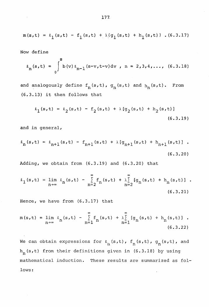
177.
m (s It) = R.l (s It) - f 1 (s It) +. A.{ 9 1 (s, t ) + hI (s, t)} • (6. 3 • 1 7 )
Now define
s
tn(s,t) = J b(vltn_1 (s-v,t-v)dv , n = 2,3,4, .•. , (6.3.18) o
and ~nalogously define fn(s,t), gn(s,t) and hn(s,t). From
(6.3.13) it then follows that
R. 1 (s,t) = R. 2 (s,t) - f 2 (s,t) + A[g2(s,t) + h 2 (s,t)]
(6.3.19)
and in general,
(6.3.20)
Adding, we obtain from (6.3.19) and (6.3.20) that
00 00
R. 1 (s,t) = ~~: R.n{s,t) - nI2
f n (S / t) + ~I2[gn(S,t) + hn(s,t)].
(6.3.21)
Hence, we have from (6.3.17) that
00 00
m (s, t) = 1 im R. (s, t ) - L f (s , t ) + A L [ g (s , t ) + h (s 1 t)] . n+oo n n=l n n=l n n
(6.3.22)
We can obtain expressions for R. (s,t), f (s,t), g (s,t), and n n n h (s,t) from their definitions given in (6.3.18) by using n
mathematical induction. These results are summarized as fol-
lows:

178.
S
9. (S,t) = I b(n} (v)m(s-v,t-v)dv n
v=o
S
f (s,t) = J ben) (v)m1(s-v,t-v)dv n
v=O
s
gn(s,t) '-A(t-s} J b(n-l) (V)Bc(t-v)dv = e
v=O
and
s
h (s,t) = f b(n-l) (v)h1(s-v,t-v)dv n
v=O n = 2,3,4, •••• (6.3.23)
To determine lim i (s,t), we must find lim ben) (v) for fixed n
n~oo n~oo
v such that 0 < v < s. We know that
and hence,
J b{t)dt ~ 1 o
Ib* (z) I = I f e-zt b(t)dtl < 1 o
(6.3.24)
for Re(z) > O. From the convolution property of the Laplace
transform, we have that
(6.3.25)
From (6.3.24) we see that

179.
lim [b* (z)]n = 0 (6.3.26) n+cc.
which implies by (6.3.25) and the uniqueness property of the
Laplace transform that
lim ben) (v) = 0 , a.e. (6.3.27) n+oo
Therefore,
lim t (s, t) = 0 , a.e. n (6.3.28) n+oo
Combining the above results we see that
t-s m(s,t) = e-A(t-s) Be(t) + AJ e- AV b(s+v) F02 (t-s-v)dv +
v=O
s t-s + A I J b (n) (v) dv
n=l v=o J e -AU b(s+u-v) F02
(t-s-u)du +
u=o
s + Ae- A (t-s) I J b Cn) (v)B
c (t-v)dv -
n=l v=o
s
I J ben) (v)m1(s-v,t-v)dv n=lv=o
(6.3.29)
It tedious but not difficult to show that (6.3.29) sat-
isfies (6.3.13).
We now direct our attention to the task of obtaining- an
expression for m1(s,t) which will complete the analysis of

180.
m(s,t). To do this we shall need the auxiliary quantity
f 01 {s,t)ds dt defined as the probability that
(i) first passage to +1 occurs during (t,t+dt) given
S(O) = 0; and
(ii) the last negative step prior to time t occurs during
(t-s-ds 1 ts) ;
given that a transition from +1 to 0 takes place at time
t = O.
The contributions of cases (a) and (b) in (6.3.4) to
ml(s,t) are given in (6.3.5) and (6.3.6), respectively, in
terms of known quantities. We shall obtain the contribution
of case (c) in (6.3.4), however, in terms of fOl(s,t) and
subsequently derive fOl(s,t) in terms of known quantities.
Case (c) implies a first passage to +1 at time s and a last
negative step at some time s - v, 0 < v < s. To satisfy (1)
and (2) in the definition of ml(s,t), given by (6.3.1), no
first passage to +2 can take place during (s,t). Therefore,
the first step taken during (s,t) must be a negative one
unless, of course, no steps occur during (s,t). Therefore
the contribution of case (c) to m1(s,t) can be expressed as
s B (v+t-s) t-s
J c e-A(t-s) + f b(v+u) -Au
. fOl (v, s) { Be (v) u--O Be (v) e F 02 (t-s-u) du}dv. v=O
(6.3.30)
Combining (6.3.30) with (6.3.5) and (6.3.6), we have

181
t-s
m1(s,t) = e~At Be(t) + Ae~AS J b(v+s)e~AV F02 (t-s-vldv +
v=O
+ Js B (v+t-s)
c -A (t-s) f 01 {v,s){ B (v) e +
c v=O
(6.3.31)
t-s
+ J u=O
b (v+u) -A u B (v) e F02 (t-s-u)du}dv.
c
To complete the analysis of ml(s,t), we need to deter
mine fOl(s,t). To do this it will be convenient to use the
quantity q (s,t)ds, r = 1,2,3, ••• , defined as the probabil-r
ity that, given a transition from +1 to 0 at time t = 0,
(i) s (t) = -ri
(ii) no first passage to +1 takes place during (O,t); and
(iii) the last negative step prior to time t occurs during
(t-s-ds, t-s) .
We define
q (O,t) -r = lim q (s,t)
s+O -r (6.3.32)
and interpret q (O,t)dt to mean the probability of events -r
(i) and {ii} above and that the last negative step prior to
time t occurs during (t-dt,t), i.e., just prior to time t.
We can no\v express fOl (s,t) in terms of q_r(O,t) and
then we shall derive the Laplace transform. of q_r(O,t). To
see the connection between fOl(s,t) and q_r(O,t), we note

182.
the position of the particle at the time of the last nega
tive step prior to first passage to +1 at time t. It is
then clear that
fOl (s,t) = Ae- AS B (s) c I (6.3.33)
r=l
for all s such that 0 < S < t. We note that if the particle
takes its last negative step prior to time t at time t - s
and S(t-s) = -(n+r-l), r = 1,2, •.• , then in order that a
negative step occur at time t and S(t+dt) = -r, n positive
steps must occur during the remaining interval (t-s,t).
Upon consideration of all possible positions of the particle
at the time of the last negative step prior to time t, we
obtain
t
q-l (O,t) = b(t)e-At
+ J I q_n(O,t-slb(sl o n=l
and
q (O,t) -r =)
t (Xl (As)n -AS I q_ (n+r-l) (O,t-s)b(s) n! e ds
n=O
(6.3.34)
r = 2,3,4, •••. (6.3.35)
Defining
* q (O,z) = -r
it follows that
(Xl
o J e -zt q(O, t) dt , -r (6.3.36)

and
where
183,
* * q-1 (0, z) = b (A+Z) + l q-n (Q I z.l An (z) n=l
CD
* \' * q (O,z) = L q_ (n +r-l) (0, Z ) An (z) -r n=O
co
An(Z) = f e-(Z+A)t (At)n b(t)dt n!
o
(6.3.37)
(6.3.38)
(6.3.39)
We now apply the method of difference equations to
(6.3.37) and (6.3.38) to obtain the Laplace transform of
q_r(O,t) which will complete the derivation of fOl(s,t). We
seek a solution of the form
* q (O,z) = -r
co
L A.y.r . 1 1. 1. 1.=
(6.3.40)
* r In order for q (O,z) = y to be a particular solution of -r
(6.3.38), it follows that y must satisfy the equation
Y = L An(Z)yn = n=O
co
* b (Z+A-AY) (6.3.41)
* For fixed t, L g (Olt) is bounded and hence q (O,z) r=l -r -r
must be bounded for all possible values of r. In order that
* q_r(O,z) be of the fonn given in (6.3.40) and remain bounded,
we must have Iy. I < I for all values of i. Upon application 1.

184.
of Rouche's theorem, we can show that there exists a unique
root y which lies within the unit circle and satisfies
(6.3.41). Therefore, the general solution of (6.3.34) and
(6.3.35) is given by
* r q (O,z) = Ay , r = 1,2,3, •••• -r (6.3.42)
From (6.3.34) it follows that
A = 1 (6.3.43)
and hence,
* r q (O,z) = y , r = 1,2,3, .•• , -r (6.3.44)
where y is the root of equation (6.3041) with smallest abso
lute value. Noting that equation (6.3.41) is identical to
(2.2.13), it follows that q_l(O,t) is equal to the probabil
ity density function for the length of the busy period in
the M/G/l queuing process given in (2.2.17). We can write,
therefore,
q-l (0, t) (6.3.45)
From (6.3.44) and the convolution property of the Laplace
transform, we obtain
q (0 It) = q-l (r) (0 It) -r (6.3.46)

185·
This completes the derivation of q_r(Q,t} and the analysis
of m(s,t).
Altho.ugh it can be shown that flO(t) for oo2/M/G is iden
tical to the busy peried density for M/G/l, given in (2.2.17),
nevertheless, it is not obvious that the function q_l(O,t)
and the busy period density functien fer H/G/l should be
equal. The event for which q-l (0, t.) is the corresponding
probability density function and the event first passage to.
o at time t given S(O) = I appear to be quite dissimila~ and
no explanation for the cemmen distributien ef these two
events has been feund. A similar phenemenen eccurs in the
random walk oo2/GI / M, as will be shown in the next Section.
As a partial check on our analysis, we now show that
the expressiens for ml(s,t) and m(s,t) given in (6.3.31) and
(6.3.29), respectively, agree with the results given in
Chapter III for the case in which positive and negative
steps eccur according to two independent Poisson streams
with means A and ~, respectively.
First of all, by letting bet)
find, with the aid of (2.3.1),that
and hence,
-TIt = ~e t-" in (6 • 3. 45), we
(6.3.47)
(6.3.48)

186.
where frO(t) is given in (3.2.16). By (6.3.33) we then have
fOl (s,t) ()()
= e-·(A+1-l) s 1: r=l
A (As) r r frO (t-s) • (6.3.49)
By substitution in (6.3.3l) of the quantities fOl(s,t) given
by (6.3.49) and bet) = pe-l-l t , we find that
t-s
) '\ e- (A +l-l ) t + '\ lIe- (A +l-l ) s f e- (A +J.l ) v ( ) d m1 (s,t = A A~ F02 t-s-v v +
v=O
s + Ae-(A+11) (t-s) J e-(A+11)V ~ f (s-v)dv +
t... rO O r=l v=
t-s
f e - 0.+11) u x F 02 (t-s-u)du.
u=O
(6.3.50)
We recall from Chapter III that the Laplace transforms of
frO(t) and F02 (t) are denoted by ¢rO(z) and ~02(z), respec
tively. An expression for ¢rO(z) can be obtained from
(3.2.13) by symmetry, and ~02(z) is given by (3.2.18).
Using the quadratic relationship given in (3.2.9) together
with (3.2.18), we obtain
(6.3.5l)
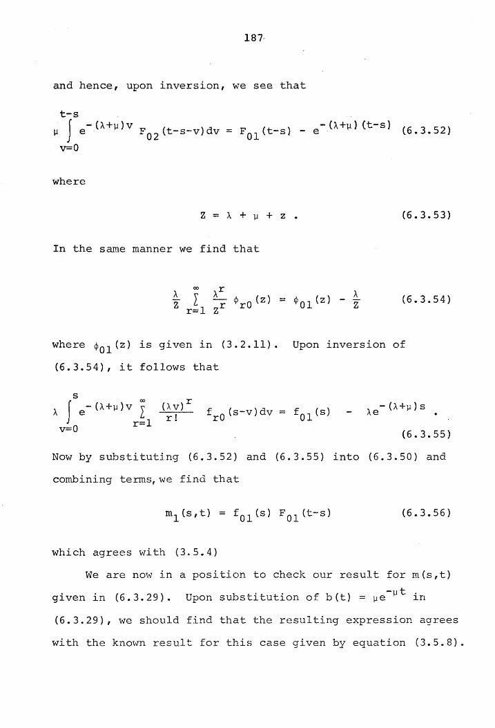
187·
and hence, upon inversion, we see that
t-s . J - (A+11)V 11 e· F02 (t-s-v)dv = F01 (t-s) - e-(A+11) (t-s) (6.3.52)
v=0
where
Z = A + 11 + Z •
In the same manner we find that
A CP01 (z) - Z
(6.3.53)
(6.3.54)
where 901 (z) is given in (3.2.11). Upon inversion of
(6.3.54), it follows that
s A J e-(A+l1)V I
r=l v=0 (6.3.55)
Now by substituti.ng (6.3.52) and (6.3.55) into (6.3.50) and
combining terms,we find that
(6.3.56)
which agrees with (3~5.4)
We are now in a position to check our result for m(s,t)
given in (6.3.29). Upon substitution of bet} = 11e-11t in
(6.3.29), we should find that the resulting expression agrees
with the known result for this case given by equation (3.5.8).

188.
After making this substitution, using (6.3.56) and summing,
we find immediately that
t-s
m(s,t) = Ae~A(t-S) e-~t + A~e-~S J e-(A+~)V F02
(t-s-v)dv +
o
t-s -~s J e-(A+~)U + A~[l - e ] F02 (t-s-u)du +
u=O
- (A+~) (t-S) -A (t-S) -~t + A[e - e e] -
s
- ~FOl(t-s) J f 01 (s-v)dv ·
v=O
Now using equation (6.3.52) and the fact that
~fOl(t) = AflO(t), it follows from (6.3.57) that
m(s,t) = AFOl (t-s) FIO(s)
(6.3.57)
(6.3.58)
which agrees with (3.5.8). We have succeeded in showing
that the general results derived in this section agree with
the known particular cases given in Chapter III.
6.4 First-Passage Time from m to n and the Time of
Occurrence and Magnitude of the
First Maximum for oo2/GI/M
We assume in this Section that the intervals between
positive steps are independently and identically distributed

189
with distribution function A(t) and probability density func-
tion aCt) while negative steps occur in a Poisson stream with
parameter 11.-
As before, we let fmn(t)dt denote the probability that
first.passage from m to n occurs during (t,t+dt) given that
t = 0 is a renewal epoch, i.e., at t = 0 a transition from
m - 1 to m takes place. Again, we consider only fOn(t),
n = 1,2,3, ••• , since
fmn (t) = f 0 , n -m (t) , n = m+ 1, m+ 2 • • • • (6.4.1)
We shall derive an expression for fOn(t) using the fact
that the times at which positive steps occur are renewal
epochs. In order that a first passage to n may take place
at time t, n = 1,2, ••• , at least n positive steps must occur
during the time interval (O,t). If r negative steps occur
prior to the first positive step, then the particle must
make a first passage from -(r-l) to n during the remainder
of the interval (O,t). Consequently, we can write
t
-~t J e-~x ~ fOl(t) = a(t)e + a(x) L x=o r=l
and
t
(].lx) r r! fOr(t-x)dx •
(6.4.2)
fOn(t) = J a(x)e-)JX I O r=O
r (~x) • r! fO,r+n-l (t-x)dx ,
X= n = 2,3,4, •••. (6.4.3)
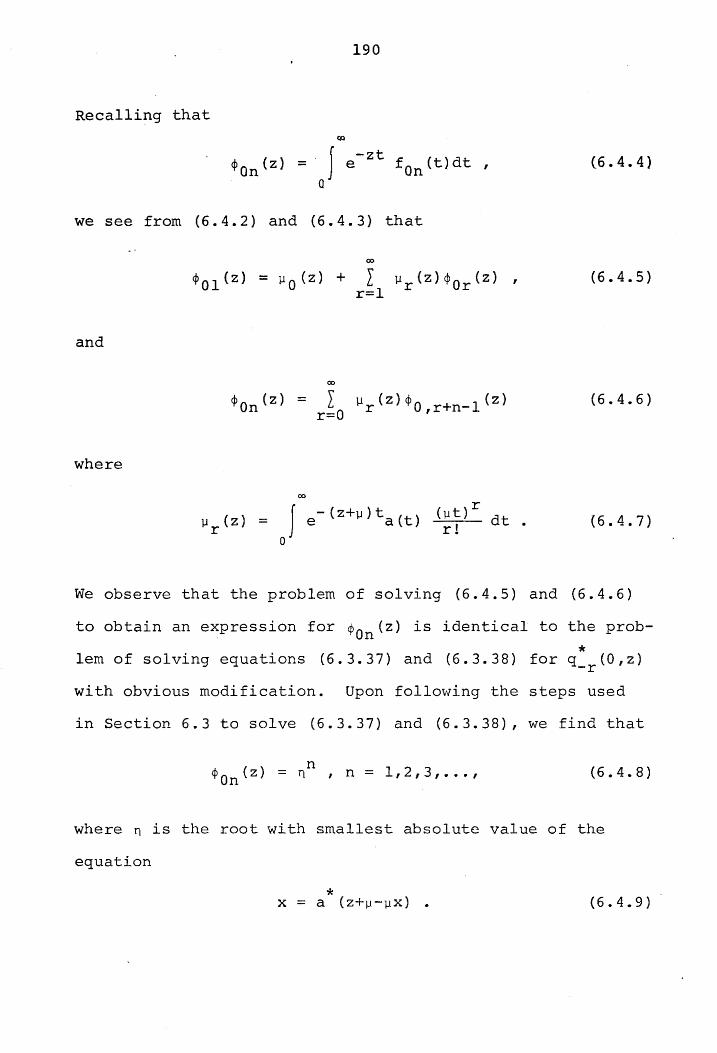
190
Recalling that <lCI
. J e-zt ~On(z) = fOn(t)dt ,
Q
we see from (6.4.2) and (6.4.3) that
and
where
00
~On(Z) =
00
~r(z) = J e-(z+~)ta(t) (~~)r dt . o
(6.4.4)
(6.4.5)
(6.4.6)
(6.4.7)
We observe that the problem of solving (6.4.5) and (6.4.6)
to obtain an expression for ~On(z) is identical to the prob
* lem of solving equations (6.3.37) and (6.3.38) for q (O,z) -r
with obvious modification. Upon following the steps used
in Section 6.3 to solve (6.3.37) and (6.3.38), we find that
n ~On(z} = n , n = 1,2,3, ... , (6.4.8)
where n is the root with smallest absolute value of the
equation
(6.4.9)

191
As before, an application of Lagra!1ge's theorem given in Sec-
tion 2.2 yields the result
m-l Cpt) I a (m) (t) •
m. (6.4.10)
By (6.4.8) and the convolution property of the Laplace trans-
form, we have
(6.4.11)
We note that if A(t) represents the distribution of
service times and B(t) = 1 - e-~t is the distribution of the
length of time between successive arrivals, then the expres-
sian for the busy period density for the M/G/l queuing
process given in (2.2.17) is identical t.o (6.4.10). In
Section 6.2 we noted that for the walk 002/M/G, the expres-
sian for fOl(t) given in (6.2.15) is identical to the busy
period density for the GI/M/l queuing process with obvious
modification. For the random walks 00 2/M/G and 002 /GI/r~, the
first-pass time density fOl(t) is identical to the busy
period density for M/G/l and GI/M/I, respectively. There
fore, we see from the preceding remarks that for 002/M/G we
can obt.ain an expression for f01Ct) from the expression for
fIO(t) for oo2/GI/ M and vice-versa. The same is true with
regard to obtaining flOCt) for oo2/M/G from fOI(t) for
oo2/GI/M and vice-versa.
If qi(O,t)dt is defined as the joint probability that

192
a positive step occurs during (t-dt,t), Set) = I, and no
first pass~ge.to -1 has occurred during (O,t), then it is
easily shown that for ~2/GI/M qiCO,t) = fOlCt) given by
(6.4.10). This result corresponds to the equality of
2 Q_1(O,t) and flO(t) for 00 /M/G as discussed in Section 6.3.
As remarked in Section 6.3, no satisfactory probabilistic
explanation of these identities has been found.
To derive mk(s,t) and m(s,t), as defined at the begin
ning of Section 6.3, we note that the first maximum during
(O,t) must occur at the time of a positive step, i.e., at a
renewal epoch. Moreover, if the first maximum is to occur
at time s and be of magnitude k, then by the definition of
first maximum given in Section 6.3, a first passage to k
must occur at time s and no first passage from k to k + 1
may occur during the remaining time interval (s,t). Con-
sequently, we can write
and
where
m(s,t) = L mk(s,t) , k=1
t
F01(t) = 1 - J f01(x)dx o
(6.4.12)
(6.4.13)
(6.4.14)

193.
Evidently, for the case aCt) =. Ae-At,.equations (6.4.12)
and (6.4.13) will agree with (3.5.4) and (3.5.8), respec-
tively, if the expression for fQl(t). given in (6.4.10) agrees
with (3.2.14). By letting aCt) = Ae- At in (6.4.10) and apply-
ing the series expansion for the modified Bessel function of
the first kind given by (2.3.1), we find that (6.4.10) be-
comes
1/2 - (A+ll) t II (2t~) = pet
which agrees with (3.2.14).
(6.4.15)
This completes the analysis of first-passage times and
first maxima for oo2/M/G and oo2/G1/ M• Unfortunately, the
corresponding results for sojourn times and returns to the
origin for these partial generalizations of oo2/M/M are not
as easy to obtain, and there is no progress to report in
this area as yet. We can make an extension of the sojourn
time results for the M/M:/l queuing system to the M/G/l and
GI/M/l systems, hO~lever, as will be shown in next sec-
tion.
6.5 The Two-State Sojourn Time Problem for the !'1/G/l
and Gr/M/l Queuing Processes
Consider, first of 1, the H/G/l queue where it is
assumed that arrivals occur in a Poisson stream with param~
eter A, and service times are independently and identically

194
distributed with distribution function B(t) and probability
density function bet). We assume,as usual, that t = Q is
a renewal epoch, i.e., a transition from +1 to 0 occurs at
t ~ a and thus S(O) = O. As in the walk ro2 /M/G, we shall
use the fact that the departure times are renewal epochs in
order to derive the probability
PB(S,t)ds = Pr{s < aBet) < s+ds I S(O) = a} (6.5.1)
given that t = 0 is a renewal epoch. The notation used here
has been discussed in detail in Sections 4.1 and 4.2. As
defined in Section 4.5 for the M/M/l queue, we say that the
system is in state B at time t if Set} > 0, i.e., if the
server is occupied.
There is one important difference between oo2/M/G and
the M/G/l queuing process which simplifies the analysis of
the sojourn density defined in (6.5.1). In the queuing proc
ess, the probability that a departure occurs while no cus
tomers are present in the system is equal to zero. Conse
quently, when a customer arrives and finds no one in the
queue, his service time is independent of the length of time
which has elapsed since the previous custorner completed ser
vice, i.e., his service time is independent of the length
of the preceding idle period. As a result, the length of
the busy period, or first-passage time from +1 to 0, is also
independent of the length of the preceding idle period. In

195.
effect, therefore, the process renews itself not only when
a departure occurs but each time a busy period begins as
well.
Making use of the fact that epochs of service comple-
tion and the times when a busy period is initiated are re-
newal epochs, we see that PB(s,t) satisfies the equation
t-s -A (t-s) f -AX -A (t-s-x)
PB(s,t) = Ae FlO(S) + A e flO(s)e dx + o
t-s s
+ f Ae-AXdx f f10(Y) PB (5-y,t-x-y)dy = o 0
(6.5.2) t-s s
+ 'J e-Axdx J flO(y) ( t }d I\. PB s-y, -x-y Y o 0
provided that 0 < s < t. The first-passage time density
flO(t) is, of course, the same as the busy period density
function for MIGII given in equation (2.2.17)
We note that (6.5.2) coincides with (4.2.19) we let
-At get) = Ae and h(t) = fIO(t). From (4.2.20) we see that
the expression
( t) = e- A (t-s) ~ [A L\ (t-s) ]n-l [F (5) - F (s)] + PB s, n~1 (n-I) ! nO n-l,O
+ [A(t~~)ln fi~) (5)] (6.5.3)

196.
satisfies (6.5.2), where
and
t
FnO{t) = 1 - J fi~) (x)dx Q
Faa (t) = a •
(6.5.4)
{6.5.5}
Since S(O) = 0, the server cannot remain busy through-
out the entire interval (O,t) and hence,
(6.5.6)
On the other hand, if no customers arrive during (O,t), the
server will not be busy at all. Therefore,
(6.5.7)
From (4.2.21) we find that distribution function PB(s,t)
is given by
s -A(t-s)
IX)
[A (t-s) J n ) f (n) (x) dx PB(s,t) = e l n=O n1 10
(6.5.8)
= Pr{O < aB
(t) < s} . - -
We can also express PB(s,t) and PB(s,t) in terms of the
Laplace transforms of flOCt) and FlO(t) denoted by ~lO(z)
and ~lO(z)f respectively. The resulting expressions are

given by
PB
(s,t)
and
PB(s,t)
-A (t-s) = e·
= e -A (t-s)
1 21Ti
1 21Ti
197.
J e ZS A(t-s)~lQ(z} -- e dz
Z (6.5.9)
J zs· {e
A(t-s)~lO(z) [1 + e
C2 (6.5.10)
+ A {l - <P10(z)}] l}dz - - , Z
where C1 ,C2
are the usual Laplace inversion contours.
The analysis for the GI/M/l queue is more difficult.
Although the times at which arrivals occur constitute renewal
epochs, the probability that an arrival occurs at any given
time always depends on the amount of time which has elapsed
since the previous arrival. We can, however, derive an in
tegral equation satisfied by pill (s,t) where
p~l) (s,t)ds = Pr{s < GB
(t) < s+ds I S (0) = l} , (6.5.11)
given that a transition from 0 to +1 occurs at time t = 0 so
that t = 0 is a renewal epoch. We assume that interarrival
intervals,or lengths of time between arrivals, are independ-
ently distributed with a general distribution function ACt)
and corresponding probability density function aCt). We
define A (t) by c
Ac (t) = 1 - A (t) • (6.5 .. 12)

198
We shall give an expression for p~l} (s,t) in terms of
flO (s,t)dsdt defined as the joint probability that
(i) first passage from +1 to a occurs during (t,t+dt)
given that S(O) = 1 and an arrival occurs at t = 0;
and
(ii) the last previous arrival occurred during
(t-s-ds,t-s), 0 < s < t.
By considering all possible combinations of times when first
passage from 1 to 0 and the last previous arrival could occur
in order that s < aBet) < s+ds, we see that p~l) (s,t) sat
isfies the equation
p~l) (s, t) =
s
+ ~J e-~v {a(t-s+v) FlO (s-v) +
v=Q
t-s
+ f a(u+v) p~l) (s-v,t-u-v)du}dv + o
s v
J J {a(t-s+u) + flO(u,v) A (u) FlO (s-v)
v=O u=Q c
t-s
(6.5.13)
+ J y=O
a (y+u) PB(1 ) (s-v,t-y-v)dy}dudv, Q < s < t • Ac(U)
Equation (6.5.13) takes into consideration the following
mutually exclusive possibilities:

199
(i) first pass~ge from +1 to Q occurs at time s and last
arrival occurred at time t = 0;
(ii) first pass~ge from +1 to Q occurs at time s and the
last arrival occurred at time s - U , Q < u < Si
(iii) first passage from +1 to 0 occurs at time v,
o < v < s, and the last previous arrival occurred at
timet = 0; and
(iv) first passage from +1 to 0 occurs at time v,
o < v < s, and the last previous arrival occurred at
time v - U, 0 < U < v.
Since S(O) = I, the server cannot remain idle through-
out the interval of time (O,t) and hence,
(6.5.14)
If no first pass from 1 to 0 occurs, however, the server
remains busy throughout (O,t). Therefore,
Pr{oB(t) = t} = FlO (t)
t (6.5.15)
= 1 - J flO (x)dx 0
For completeness we give an expression for f10(s,t).
The derivation £ollo\'1s steps analogous to those used in Sec-
tion 6.3 to derive f01(s,t) for =2/M/G and there we omit
the details. In fact, the desired expression for £10(s,t)

200
can be obtained directly from the expression for fOl(s,t)
given iri (6.3.33) with obvious change in notation and inter-
change of the roles of the positive and negative steps.
Therefore, we simply state this result as
00
flO (s,t) -liS \'
= ue t"" Ac (s) L n=l
r n+l (O,t-s) , (6.5.16)
where
00 (ll t) m-l a(m) (t) r 2 (0, t) = -lIt 2 e rn! ,
m=l (6.5.17)
and
rn(O,t) = r~n-l) (O,t) , n = 2 I 3 , 4 , . . . . (6.5.18)
As a partial check on our analysis, we shall show that
(6.5.13) yields the known results in Chapter IV for the case
of independent, negative exponentially distributed inter-
arrival and service times. Using the fact that for the M/M/l
queuing process we have
s
p~l) (s,t) = e -A (t-s) flO (s) + J flO (x)p~O) (s-x,t-x)dx
o (6.5.19)
together with equation (4.2.20), it can be shown that

20~
t-s s
+ AJ e-AYdy J flO(V)p~l) (s-v,t-v-y)dv ,
y=O v=O (6.5.20)
where FnO(t) is defined by (6.5.4) and (6.5.5), n = 0,1,2, ••.•
Therefore, (6.5.13) should agree with (6.5.20) for the case
when interarrival and service times are negative exponentially
distributed with parameters A and ~, respectively.
Letting aCt) = Ae- At in (6.5.17), we find that
.;- - (A+~) t II (2t~) r 2 {0,t) = p e t
(6.5.21)
= pflO (t) ·
Therefore, by (6.5.16) and (6.5.18) we have
flO(s,t) = ( 's)r () Ar! fl~ (t-s) • (6.5.22)
Upon substitution of (6.5.21) and (6.5.22) into (6.5.13),
we obtain
p~ 1) (s, t) = -(A+~)S -A(t-S) ~e . e +
s
(AU)r () flrO (s-u)du + r!
+ A~J e-(A+~)V{e-A(t-s)F (s-v) + 10
v=o
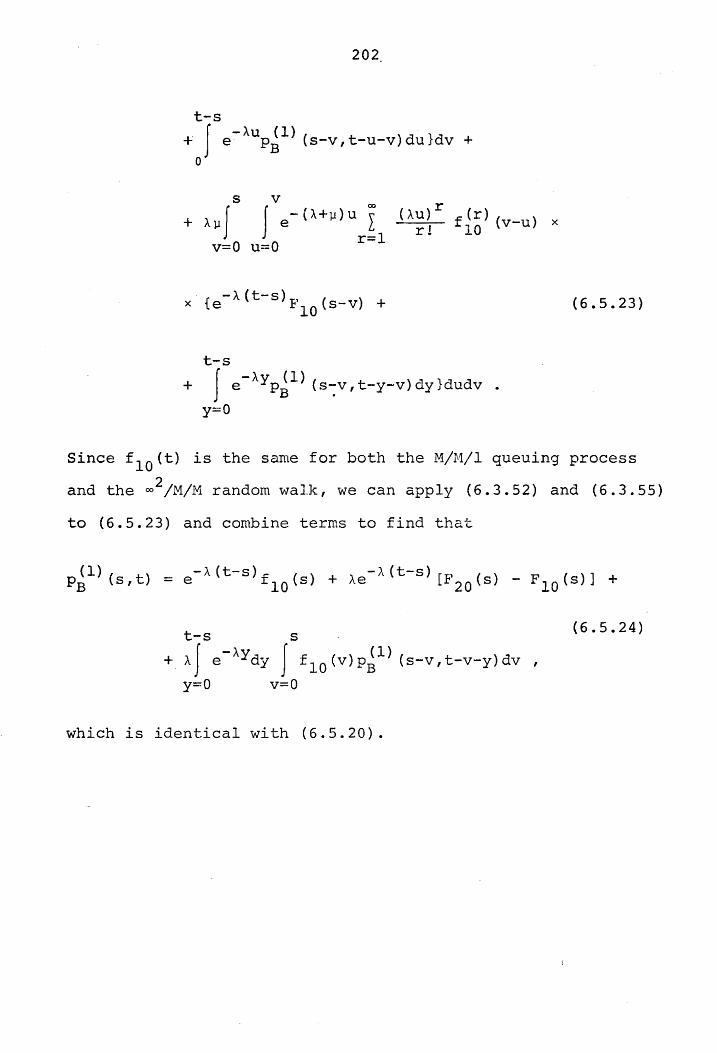
202
t-s
I -AU (I) + e PB
(s-v,t-u-v)du}dv + o
s v
+ A~f J e-{A+~)U I r=l v=o u=o
x' ie-A (t-s) F (s-v) + 10
t-s
( AU)r () f r (v-u) x
r! 10
+ f e-AYp~l) (s~v,t-y-v)dy}dudv ·
y=O
(6.5.23)
Since flO(t) is the same for both the MIMII queuing process
and the oo2/M/H random walk, we can apply (6.3.52) and (6.3.55)
to (6.5.23) and combine terms to find that
p~l) (s,t) == e- A (t-s) f (5) + Ae -:\ (t-s) [F (s) - FlO (5)] + 10 20
t-s s (6.5.24)
+ AJ e-AYdy f f10(v)pi1 ) (s-v,t-v-y)dv ,
y=O v==O
which is identical with (6.5.20).

CHAPTER VII
SUMMARY AND CONCLUDING P£MARKS
This disser~ation contains a study of certain topics re
lated to the random walk which proceeds by steps of ±l occur
ring at random time intervals. In general it is assumed that
the intervals of time between steps of the same kind are in
dependently and identically distributed. This model may be
specialized to the queuing process by placing a reflecting
barrier at the origin so that the displacement Set) of the
random walk at any time t is non-negative.
Throughout most of the dissertation it is assumed that
the steps of +1 occur according to two independent Poisson
streams with parameters A, ~, respectively. Under this as
sumption we designate the single-server queuing process by
the usual notation M/M/l, and we denote by oo2/M/M the unre
stricted random walk in which Set) may range over the entire
set of positive and negative integers including zero. The
letter M is used here to denote a negative exponential dis
tribution. Where it is assumed that the lengths of time be-
tween steps of +1 or between steps -1 are independently
distributed according to a general distribution, the notations
oo2/GI/M and oo2/M/G are used.
The study begins necessarily, because of its fundamental
impo~tance, with a discussion of the first passage time to
203

204,
an arbitrary state n given that the initial displacement S(O)
is equal to m. Explicit expressions for the probability den
sity function of the first-passage time from m to n are given
for oo2/M/M. In Chapter VI, this result is extended to the
more general random walks oo2/M/G and oo2/GI/M, an extension
which appears to be new. For the M/M/I queuing process,
Bailey [3] gives the distribution of the first-passage time
from m to n for the case m > n. In this dissertation new re
sults are given for the case m < n.
Intimately connected with the first-passage time problem
is the problem of the time of occurrence and magnitude of the
first maximum during (O,t). For the walk oo2/M/M expressions
are given in Chapter III for the joint probability and pro
bability density function of tl, the epoch of the first maxi
mum, and Set'), the maximum displacement during (Oft). The
marginal distributions of t' and S(t 1) are obtained from the
joint distribution. In Chapter VI these results are extended
to the walks oo2/H/G and ro 2/GI/M. Apparently, this extension
is new. For the walk ro 2/M/M, it is found that the asymptotic
distribution of t l can be expressed in terms of the stable
distribution of index 1/2 for the case A :f ].1 and in terms of
the arc sine distribution for the case A = ].1 • The asymptotic
results for the case A ~ ].1 have not been published before.
Unfortunately, an investigation of the distributional proper
ties of t' and S(tl) for the M/M/I queuing process has so
far proved unsuccessful and must therefore remain an area

20~
for future research.
In addition to the topics of first-passage time and
first maximum, Chapter III contains a study of two other ran-
dam variables, viz. the number of returns to zero during an
arbitrary time interval (O,t) and the time up to the th
r re-
turn to zero. For both oo2/M/M and the MIMll queuing process,
explicit expressions are developed for the probability of n
th returns to zero during (O,t) and the probability that the r
return to zero occurs during the small interval (t,t+dt).
Moments and moment generating functions are given as well as
asymptotic approximations valid for large values of t. Many
of the results obtained do not appear to have been published
previously.
A major portion of the dissertation,deals with the so-
called two-state sojourn time problem in which it is assumed
that at any time t the particle may be in either one of two
possible states, A and B. General expressions are derived
for the probability density and distribution functions of
the sojourn time 0 B (t) in a given state B during an arbitrary
time interval (O/t). In Chapter IV the general two-state
sojourn time result has been applied to the MIMII queuing
process in order to obtain the distribution of the busy time.
Little attention has been given previously to the application
of the sojourn time results to single-server queues with the
exception of papers by Greenberg [24] and Linhart [26]. A
similar application is made to =2/M/M to obtain the distri-

20~
bution of aBet) for the two cases:
(i) B is the set of all non-zero integers; and
(ii) B is the set of all positive integers.
In each of the three particular applications considered, the
distribution function and probability density function of the
sojourn time aBet) are expressible in terms of the modified
Bessel function of the first kind and the J-function studied
by Goldstein [22] in connection with certain diffusion pro
cesses in a non-probabilistic context. These distribution
and density functions have apparently not been expressed in
this form previously. Such expressions are more easily adap
ted for numerical computation. Also, asymptotic results for
large values of time can be obtained directly from these ex
pressions. Consequently, asymptotic formulae for the proba
bility Pr{at<oB(t)<t}, O<a<l, valid for large t, are obtained
from the explicit results for finite values of t. In most
cases these limiting forms are expressible in terms of the
stable distribution of index 1/2. Section 4.6 compares nu
merically the asymptotic approximations of Pr{at<oB(t)<t} de
veloped from our work to the approximations obtained from
Tak~cs' results [35]. In contrast to our direct approach,
Takacs' asymptotic formulae are based on the general theory
of the asymptotic behavior of sums of random variables. Al
though Takacs' results are also expressible in terms of the
stable distribution of index 1/2, our approximations are gen
erally more accurate, especially for relatively small values

20~
of time.
Chapter V contains a discussion of several results by
E. Sparre Andersen concerning fluctuations of sums of random
variables and their time-dependent analogues. These analogues
have not been mentioned in the literature with the exception
of an unpublished paper by Conolly [11]. For example, it is
found that in the oo2/M/M walk beginning at zero that t', the
epoch of the first maximum during (O,t), and 0B(t}, where B
is the set of positive integers, are identically distributed.
This result has a counterpart for non-time-dependent random
walks given by Andersen [11 and [2].
Although the volume of literature on random walks is
great, few explicit results have been published concerning
the time-dependent random walk considered in this dissertation.
In addition to the theoretical interest generated by such a
random walk, its close link with certain time-dependent ran~
dom walk models of practical interest makes it worthy of fur
ther study. For example, the application most often cited in
this dissertation is the single-server queuing process. Other
queuing systems, however, such as multi-server systems, inven
tory models characterized by a last-come first-served queue
di~cipline, and systems with arrival and service mechanisms
dependent on queue length are also examples of models in which
the time-dependent random walk is basic. In addition to queu
ing situations, the continuous-time random walk is applicable
to models used to describe population changes over a given

20~
period of time. In these models, a step of +1 corresponds to
a birth or any other addition to the population while a step
of -1 corresponds to a death or a migration from the popula-
tion.
Although many related areas for possible future research
could be suggested, the following are two of the most impor-
tant ones.
1) Instead of restricting consideration to step lengths
of ±l, one could study the time-dependent random walk
in which the step length X is a continuous random
variable. This type of model is applicable, for ex-
ample, to insurance models in which it is assumed
that claims occur at random time intervals and that
the amount X of an individual claim has a continuous
distribution. In principle these claims may be pos-
itive or negative. (For example, a death may free . the company of an obligation and increase the re-
serves.) Some aspects of such a random walk in dis-
crete time have been discussed by Conolly [10]. An
analysis of various aspects of the continuous-time
case remains to be done.
2) In this dissertation we have assumed, excep·t in Chap-
ter VI, that during the small time interval (t,t+dt),
a step of +1 or -1 occurs with instantaneous proba-
bility Adt, ~dt, respectively. For many applications,
however, it is convenient to assume that these in-

209.
stantaneous probabilities vary with time, or in the
so-called birth and death models, these probabilities
are assumed to depend on the number in the population
at time t. For a discussion of birth and death pro
cesses see [18], Chapter XVII. An attempt should be
made to extend the sojourn time results of Chapter
IV to these more general models. Such an analysis
would yield probabilistic information about the pro
portion of time that the number in the population re
mains above or below a given level.
The above is a sample of the problems remaining to be
solved in this field. The results obtained in this disser
tation should form the basis for further investigation and
generalization.

BIBLIOGRAPHY
1. Andersen, E. Sparre. nOn the Fluctuations of Sums of Random Variables," Math. Scand., 1(1953), pp. 263-285.
2. ~ndersen, E. Sparre. "On the Fluctuations of Sums of Random Variables II," Hath. Scand., 2(1954), pp. 195-223.
3. Bai ley, N. T . J . H Some Further Results in the Non - Equi-1ibrium Theory of a Simple Queue,1l J. Roy. Statist. Soc. B, 19(1957), pp. 326-333.
4. Bailey, W.N. Generalized Hypergeometric Series. Cambridge, 1935.
5. Baxter, G. and H.D. Donsker. liOn the Distribution of the Supremum Functional for Processes with Stationary Independent Increments," Trans. Am. Math. Soc., 85(1957), pp. 73-87. --
6. Churchill, R.V. Operational Mathematics. Second edition. New York, 1958.
7. Clarke, A.B. "A Waiting Line Process of Markov-Type,11 Ann. !1ath. Stat., 27(1956), pp. 452-459.
8. Cohen, J.W. "The Distribution of the Maximum Number of Customers Present Simultaneously During a Busy Period for the Queuing Systems MIGII and GI/M/1,11 J. App1. Prob., 4(1967), pp. 162-179.
9. Conolly, B.W. !fA Difference Equation Technique Applied to Simple Queue, n J. . Statis. Soc. B, 20(1958), pp. 165-167.-
10. Conolly, B. vJ. "March~ Aleatoire dont la Reparti tion de la Longueur des Etapes Suit une Loi Exponentiel1e Negative," Ann. Inst. Henri Poincare, 2(1965), pp. 173-184-. - -- ---
11. Conolly, B.W. "On Randomized Random. vJalks,1f Submitted for Publication.
12. Copson, E.T. Asymptotic Expa~sions. Cambridge, 1965.
13. Cox, D.R. Renewal Theory. New York, 1962.
210

211
14. Dobrusin, R.L. "Limit Theorems for a Markov Chain of Two States," Izvestiya Akad. Nauk ~.S.S .. R. Sere Mat., 17(1953), pp. 291-330.
15. Doetsch, Gustav. Transforms.
Guide to the Applications of Laplace New York, 1961.
16. Erdelyi, A. et al. Higher Transcendental Functions. 3 vols." New York, 1953.
17. Erdelyi, A. et ale Tables of Integral Transforms. 2 vols. New York, 195~
18. Feller, W. An Introduction to Probability Theory and its AppIIcations. Vol. (second edition).. New York, 1957.
19. Feller, W. An Introduction to Probability Theory and its AppIIcations. Vol. II. New York, 1966.
20. Feller, W. "Infinitely Divisible Distributions and Bessel Functions Associated with Random Walks," J. SIAM Appl. Math., 14(1966), pp. 864-875.
21. Ford, F.A.J. "On Certain Indefinite Integrals Involving Bessel Functions, It ~. of Math. and Physics_, 37{1958), pp. 157-168.
22. Goldstein, S. "On the Mathematics of Exchange Processes in Fixed Columns," Proc. Roy. Soc. A, 219(1953), pp. 151-171. -
23. Good, I.J. "The Frequency Count of a Markov Chain and the Transition to Continuous Time,tl Ann. Math. Stat., 32(1961), pp .. 41-48.
24. Greenberg, I.. IIrrhe Distribution of Busy Time for a Simple Queue," J. Ope Res. Soc. America, 12(1964), pp.. 503-504 ..
25. Heathcote, C.R. liOn the Maximum of the Queue GI/M/l," J. Appl. Prob., 2(1965), pp. 206-214.
26.. Linhart, P. B .. "AI terna ting Rene'"IJal Proces se s, vTi th Applications to Some Single-Server Problems,1I Paper read at the Fifth International Telegraphic Congress, Rockefel University, New York, June 14-20, 1967.
27. Luke, Y.L. 1962.
Integrals of Bessel Functions. New York,

212
28. Maximon, L.C. "On the Representation of Indefinite Integrals Containing Bessel Functions by Simple Neumann Series," Proc. Am. Math. Soc., 7(1956), pp. 1054-1062.
29. Nehari, Zeev. Conformal Mapping. New York, 1952.
30. Prabhu, N.U. and Inventories. New York, 1965.
31. Saaty, Thomas L. Elements of Queuing Theory. New York, 1961.
32. Smith, W.L. and W.E. Wilkinson (ed.). the Symposium on Congestion N.C., 1965. --
Proceedings of Chapel Hill,
33. Spitzer, F. Principles of Random Walk. Princeton, 1964.
34. Takacs, L. liOn Certain Sojourn Time Problems in the Theory of Stochastic Processes,lI Acta. Math. Acad. Sci. Hung., 8(1957), pp. 169-191.
35. Tak~cs, L. "On Limiting Distributions Concerning a Soj ourn 'rime Problem," Acta. Math. Acad. Sci. Hung., 8(1957), pp. 279-294.
36. Takacs, L. Introduction to the York, 1962.
of Queues, New
37. u.S. National Bureau of Standards. Handbook of Mathematical Functions. Applied MathematicsSeries
, Government Printing Office, Washington, D.C., 1964.
38. Wagner, K.W. Operatorenrechnung. Barth, Leipzig, 1940.
39. Watson, G.N. Theory of Bessel Functions. New York, 1945.
40. Whittaker, E.T. and G.N. Watson. A Course of Modern Analysis. Cambridge, 1952.
41.. Widder, D.V. The Laplace Transform. Princeton, 1946.

VITA
Allen Edward Gibson, the youngest of the three sons of
Mr. and Mrs. Henry T. Gibson, was born in New Milford, Connec-
ticut, on December 18, 1942. He attended the public schools
of New Milford and graduated from New Milford High School in
June, 1960.
In September, 1960, Mr. Gibson entered Denison University,
Granville, Ohio. While at Denison he majored in mathematics
and received the Bachelor of Arts degree in June, 1964. In
September, 1964, Mr. Gibson began study for the Master of Sci-
ence Degree in Mathematics at Case Institute of Technology,
Cleveland, Ohio. He received this degree in June, 1966.
Mr. Gibson married the former Katherine Measamer on Au-
gust 20, 1966.
In September, 1966, he entered the Department of Statis-
tics at Virginia Polytechnic Institute, Blacksburg, Virginia,
as a candidate for the degree of Doctor of Philosophy. Upon
completing requirements for this degree, he will begin ernploy-
ment with Bell Telephone Laboratories, Whippany, New Jersey.
Allen E. Gibson
213

SOME ASPECTS OF TIME-DEPENDENT
ONE-DIMENSIONAL RANDOM WALKS
Allen E. Gibson
Abstract
This dissertation contains a study of related topics
connected with the one-dimensional random walk which proceeds
by steps of +1 occurring at random time intervals. In gen
eral it is assumed that these intervals are identically and
independently distributed. This model may be specialized to
the queuing process by inserting a reflecting barrier at the
origin so that the displacement S(t) of the random walk at
any time t is non-negative.
Throughout most of the dissertation it is assumed that
the time intervals between steps of the same kind are inde
pendently and negative exponentially distributed with non
time-dependent parameter A for positive steps, and ~ for
negative steps. under this assumption we designate the sin
gle-server queuing process by the usual notation ~1/M/l.
Using an obvious extension to the queuing notation, we denote
by oo2/M/M the unrestricted walk in which Set) may range over
the entire set of positive and negative integers including
zero.
TOpics of classical interest are discussed such as first
passage times, first maxima, the time of occurrence of the

rth return to zero, and the number of returns to zero during
an arbitrary time interval (O,t). In addition to the dis
cussion of these topics for w2/M/M and MIMII, probability
density functions are obtained for the first-passage times
and the epoch of the maximum on the assumption that
time intervals between steps of +1 have a general distribu
tion and steps of -1 occur in a Poisson stream and vice-versa.
These more general expressions are new.
Special emphasis is placed on the two-state sojourn
problem in which it is assumed that at any ti.me t, Set} be
longs to one of two possible states, A and B. The distribu
tion of the sojourn time aBet) in a given state B during the
arbitrary time interval (O,t) is given. The general result
for the distribution of aBet) is applied to the MIMII queu
ing process to obtain the distribution of the busy time. A
similar application is made to the walk co2/r4/M to obtain the
distribution of aBet) for the two cases:
(i) B is the set I non-zero integers; and
(ii) B is the set I positive integers.
New expressions are given the distribution function of
aBet) in all three cases. New asymptotic formulae for these
cases are derived and compared nlli~erically with those ob
tained by Takacs using different methods.
For the more difficult sojourn time problem assuming
three possible states, A, BI , and B2 , the joint p lity

density function of aA(t) and aB (t) is derived. This result, 1
not published before, is applied to oo2/M/M assuming that A
contains zero only and that Bl and B2 consist of the sets of
positive and negative integers, respectively.
The dissertation also includes a discussion of several
results by E. Sparre Andersen concerning fluctuations of sums
of random variables and their time-dependent analogues.