solving multi-dimensional problems of gas …tr{2139 solving multi-dimensional problems of gas...

Solving multi-dimensional problems

of gas dynamics using MATLAB R©

L. K. Antanovskii

Weapons Systems Division

Defence Science and Technology Organisation

DSTO–TR–2139

ABSTRACT

This report describes an implementation of a Godunov-type solver for gas dy-namics equations in MATLAB R©. The main attention is paid to providing ageneric code that can be easily adapted to particular problems in one, two orthree dimensions. This is achieved by employing a cell connectivity matrixthus allowing one to use various structured and unstructured meshes with-out modification of the core solver. The code has been thoroughly tested forMATLAB Version 7.6 (Release 2008a).

APPROVED FOR PUBLIC RELEASE

DSTO–TR–2139

Published by

DSTO Defence Science and Technology OrganisationPO Box 1500Edinburgh, South Australia 5111, Australia

Telephone: (08) 8259 5555Facsimile: (08) 8259 6567

c© Commonwealth of Australia 2008AR No. 014-204June, 2008

APPROVED FOR PUBLIC RELEASE

ii

DSTO–TR–2139

Solving multi-dimensional problems of gas dynamics usingMATLAB R©

Executive Summary

In many circumstances it is required to simulate blast propagation in complex three-dimensional domains in order to estimate pressure and temperature fields at some distancefrom the source of explosion. Though this is the classical problem of gas dynamics whosesolution is implemented in many commercial software packages, the use of such pack-ages is sometimes limited to a particular platform, specific mesh type and proprietaryinput/output file formats, and requires a long learning curve associated with input datapreparation (pre-processing) and visualisation of the obtained results (post-processing).At the same time commercial software may not be open to model extension and may notbe easily embedded into other systems.

This report describes an implementation of a Godunov-type solver for gas dynamicsequations in MATLAB R©. The main attention is paid to providing a generic code thatcan be easily adapted to particular problems in one, two or three dimensions. This isachieved by employing a cell connectivity matrix thus allowing one to use various struc-tured and unstructured meshes without modification of the core solver. The code has beenthoroughly tested for MATLAB Version 7.6 (Release 2008a).

The work has been performed within the “Blast Modelling for Cordon Assessment andBomb Scene Examination” research project NS 07/002.

iii

DSTO–TR–2139

Author

Leonid AntanovskiiWeapons Systems Division

Leonid Antanovskii obtained an MSc Degree with Distinctionin Mechanics and Applied Mathematics from the NovosibirskState University (Russia) in 1979 and a PhD in Mechanics ofFluid, Gas and Plasma from the Lavrentyev Institute of Hydro-dynamics (Russian Academy of Science) in 1982. Since gradu-ation he worked for the Lavrentyev Institute of Hydrodynamicsin the area of fluid mechanics. In 1991–1994 he worked for Mi-crogravity Advanced Research & Support Center (Italy) underthe auspices of the European Space Agency, being involved inthe modelling of complex physical phenomena predominantlyarising in low-gravity environment. In 1994–1995 he workedat the University of the West Indies (Trinidad & Tobago), in1996–1998 in Moldflow (Australia), and in 1998–2000 in Ad-vanced CAE Technologies (USA). In 2000–2007 he worked inprivate industry in Australia.

Leonid Antanovskii joined DSTO in February 2007 where hiscurrent research interests include development of vulnerabilityand lethality models for weapon–target interaction.

v

DSTO–TR–2139

Contents

1 Introduction 1

2 Elements of gas dynamics 1

3 The Riemann problem 3

4 Numerical model 6

5 Gas dynamics toolbox 8

6 Usage examples 16

6.1 Sod’s shock tube . . . . . . . . . . . . . . . . . . . . . . . . . . . . . . . . 16

6.2 Rotationally symmetric blast . . . . . . . . . . . . . . . . . . . . . . . . . 18

6.3 Two-dimensional blast propagation . . . . . . . . . . . . . . . . . . . . . . 21

6.4 Three-dimensional blast propagation . . . . . . . . . . . . . . . . . . . . . 26

7 Conclusion 32

References 32

vii

DSTO–TR–2139

Figures

1 Dimensionless Hugoniot–Poisson curves. . . . . . . . . . . . . . . . . . . . . . 5

2 Gas state in Sod’s shock tube. . . . . . . . . . . . . . . . . . . . . . . . . . . . 17

3 Blast waves from a spherical charge. . . . . . . . . . . . . . . . . . . . . . . . 19

4 Two-dimensional blast propagation; pressure field surfaces. . . . . . . . . . . 24

5 Two-dimensional blast propagation; temperature field surfaces. . . . . . . . . 25

6 Three-dimensional blast propagation; pressure field slices. . . . . . . . . . . . 30

7 Three-dimensional blast propagation; temperature field slices. . . . . . . . . . 31

viii

DSTO–TR–2139

1 Introduction

In many circumstances it is required to simulate blast propagation in complex three-dimensional domains in order to estimate pressure and temperature fields at some distancefrom the source of explosion. Though this is the classical problem of gas dynamics whosesolution is implemented in many commercial software packages, the use of such pack-ages is sometimes limited to a particular platform, specific mesh type and proprietaryinput/output file formats, and requires a long learning curve associated with input datapreparation (pre-processing) and visualisation of the obtained results (post-processing).At the same time commercial software may not be open to model extension and may notbe easily embedded into other systems.

MATLAB R© provides a nice environment for numerical simulation of real-world prob-lems with integrated visualisation, powerful scripting framework, and fast algorithms im-plemented. Many books are devoted to the application of MATLAB to various problemsof science and engineering (see e.g. [Danaila et al. 2007, Klee 2007, Gilat 2008]).

In this report, two compact MATLAB files (M-files) constituting the development of aGas Dynamics Toolbox (MATLAB library) are presented which are sufficient to run froma user-defined script and simulate gas dynamics problems. A robust Godunov-type solver[Godunov 1959, Richtmyer & Morton 1967, Holt 1977, Toro 1999] based on the exactRiemann solver for flux calculation between control cells is employed. Though there existmany advanced schemes for simulation of gas dynamics equations with higher accuracy (seee.g. [van Leer 1979]), the first-order accurate Godunov solver provides a highly desirablemonotone numerical scheme and is easily extendable to multi-dimensional problems. Thehistory of discovery of this algorithm based on deep insight into the physics of shock andrarefaction waves is given in [Godunov 1999].

2 Elements of gas dynamics

Let ω be a control volume with piecewise smooth boundary ∂ω oriented by inwardnormal unit vector n. The classical conservation laws of mass, momentum and energy forgas flow, written for arbitrary ω, are as follows

ddt

∫ω

ρdV =∫∂ω

ρv · n dA , (1)

ddt

∫ω

ρv dV =∫∂ω

(ρv v · n + pn) dA , (2)

ddt

∫ω

ρ

(e+

12|v|2

)dV =

∫∂ω

[ρ

(e+

12|v|2

)+ p

]v · n dA . (3)

Here t is time, ρ density, v velocity, p pressure, and e specific internal energy. Symbols dVand dA denote volume and area elements, respectively. The effect of gravity is ignored.

1

DSTO–TR–2139

Since the control volume ω is arbitrary, the integral conservation laws (1)–(3) implythe following differential conservation equations

∂ρ

∂t+∇ · (ρv) = 0 , (4)

∂(ρv)∂t

+∇ · (ρv ⊗ v + pG) = 0 , (5)

∂

∂t

[ρ

(e+

12|v|2

)]+∇ ·

{[ρ

(e+

12|v|2

)+ p

]v}

= 0 , (6)

where ∇ denotes the gradient operator, ⊗ the tensor product, and G the metric tensor.The conservative form of gas dynamics equations admits discontinuous solutions suchas shock waves and contact discontinuities. In this case temporal and spatial derivativeshave to be considered in the generalised sense. For continuous solutions such as rarefactionwaves the conservative Euler equations (4)–(6) can be further simplified to

∂ρ

∂t+ v · ∇ρ+ ρ∇ · v = 0 , (7)

ρ

(∂v∂t

+ v · ∇v)

+∇p = 0 , (8)

ρ

(∂e

∂t+ v · ∇e

)+ p∇ · v = 0 . (9)

As a consequence of equations (7), (9) and the second law of thermodynamics

θ ds = de+ pd(

1ρ

)(10)

where θ and s are the absolute temperature and specific entropy, respectively, the sub-stantial derivative of entropy vanishes:

dsdt≡ ∂s

∂t+ v · ∇s = 0 . (11)

In other words, entropy at a particle remains constant in a continuous gas flow. Note thatentropy at a particle undergoing a shock wave always increases.

The fundamental thermodynamic relations for ideal polytropic gas result in the fol-lowing state equation [Courant & Friedrichs 1948]

p = (γ − 1) ρ e (12)

where γ is the ratio of the specific heat at constant pressure to the specific heat at constantvolume. Indeed, by the definition, gas is ideal (thermally perfect) if its thermodynamicstate satisfies Clapeyron’s equation

p = Rρ θ (13)

where R is the specific gas constant defined as the ratio of the universal gas constantto the molar mass of gas (or, equivalently, the ratio of the Boltzmann constant to theaverage mass of the gas molecule). From the second law of thermodynamics (10) it is

2

DSTO–TR–2139

straightforward to deduce that the specific internal energy of ideal gas is a function ofthe absolute temperature alone. Ideal gas is polytropic (calorically perfect) if e is a linearfunction of θ, namely

e = cv θ (14)

where cv is the specific heat at constant volume. In this case the specific enthalpy h,defined by the expression h = e+p/ρ, is also a linear function of the absolute temperature

h = cp θ (15)

where cp = cv + R is the specific heat at constant pressure. These formulae result inexpression (12) with γ = cp/cv. Note that the sound speed a of a polytropic gas is givenby the formula

a =√γ p

ρ. (16)

Let us introduce the volumetric density of momentum, u = ρv, and the volumetricdensity of total energy, ε = ρ

(e+ 1

2 |v|2)

. In terms of these conserved variables theconservation laws (1)–(3) take the succinct form

ddt

∫ω

[ρ, u, ε] dV =∫∂ω

[u · n, 1

ρu u · n + pn,

ε+ p

ρu · n

]dA (17)

where

p = (γ − 1)

(ε− |u|

2

2ρ

)(18)

according to the equation of state (12).

Most numerical algorithms, including Godunov-type solvers, are based on the aboveintegral equations. The main problem is related to the correct determination of the fluxesof mass, momentum and energy through the interface separating two control volumes interms of the cell values of the conserved variables.

3 The Riemann problem

The one-dimensional Riemann problem is important for understanding the physics ofcompression and expansion waves, and provides an exact expression for fluxes between twoadjacent uniform states of gas separated by an infinite plane. The solution of the Riemannproblem is described in many texts on gas dynamics (see e.g. [Courant & Friedrichs 1948]).In this section the solution is outlined without providing full details.

Consider the propagation of a shock wave or rarefaction fan into a uniform gas inthe direction of Cartesian coordinate x with front initially positioned at x = 0. It isassumed that the gas flow does not depend on the remaining Cartesian coordinates, and

3

DSTO–TR–2139

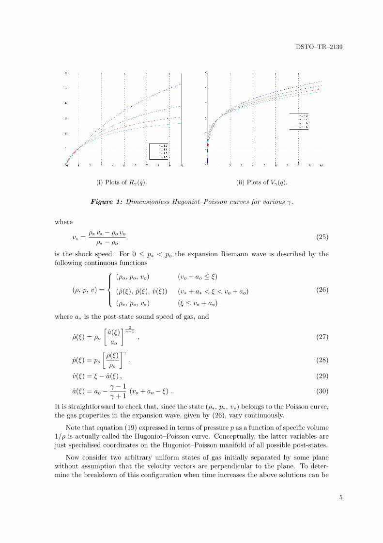
velocity field has the only nonzero component v in the x-direction. Denote given pre-stateof gas initially occupying the half-space {x > 0} by (ρo, po, vo). Let us determine all thepossible post-states (ρ∗, p∗, v∗) of gas initially occupying the complementary half-space{x < 0} and connected with the given pre-state by a shock wave or simple rarefaction fan,both propagating in the positive direction of x relative to vo. It turns out that the post-states cannot be arbitrary but form a one-dimensional manifold (curve). This curve canbe parametrised by the post-state pressure p∗, and therefore the density ρ∗ and velocityv∗ are known functions of p∗ and the pre-state (ρo, po, vo). These functions are piecewiseanalytic, described by two different expressions for p∗ > po (Hugoniot curve) and p∗ < po(Poisson curve). The Hugoniot and Poisson curves join smoothly at p∗ = po up to thecontinuous second-order derivative and form the combined Hugoniot–Poisson adiabaticcurve given by the formulae

ρ∗ρo

= Rγ

(p∗po

), (19)

v∗ − voao

= Vγ

(p∗po

). (20)

Here

Rγ(q) =

q + γ−1

γ+1γ−1γ+1 q + 1

(q ≥ 1)

q1/γ (0 ≤ q < 1)

(21)

Vγ(q) =

q − 1√γ(γ+1

2 q + γ−12

) (q ≥ 1)

2γ − 1

(qγ−12γ − 1

)(0 ≤ q < 1)

(22)

and ao is the pre-state sound speed of gas. The graphs of the functions Rγ(q) and Vγ(q)are displayed in Figure 1. In acoustic approximation of small p∗ − po (compared to po)equations (19) and (20) reduce to

ρ∗ − ρo =p∗ − poa2o

, v∗ − vo =p∗ − poρo ao

. (23)

The product ρ a is called impedance.

Note that the Hugoniot curve (q > 1) is derived from the Rankine–Hugoniot conditionsat the shock wave, whereas the Poisson curve (0 ≤ q < 1) is obtained from the exactsolution of gas dynamics equations written in terms of Riemann invariants. The gas stateis obtained as an explicit similarity solution (depending on ξ = x/t) to gas dynamicsequations. For p∗ > po the compression Riemann wave is given by the piecewise constantprofile of density, pressure, and velocity

(ρ, p, v) =

{(ρo, po, vo) (vs < ξ)

(ρ∗, p∗, v∗) (ξ < vs)(24)

4

DSTO–TR–2139

(i) Plots of Rγ(q). (ii) Plots of Vγ(q).

Figure 1: Dimensionless Hugoniot–Poisson curves for various γ.

where

vs =ρ∗ v∗ − ρo voρ∗ − ρo

(25)

is the shock speed. For 0 ≤ p∗ < po the expansion Riemann wave is described by thefollowing continuous functions

(ρ, p, v) =

(ρo, po, vo) (vo + ao ≤ ξ)

(ρ(ξ), p(ξ), v(ξ)) (v∗ + a∗ < ξ < vo + ao)

(ρ∗, p∗, v∗) (ξ ≤ v∗ + a∗)

(26)

where a∗ is the post-state sound speed of gas, and

ρ(ξ) = ρo

[a(ξ)ao

] 2γ−1

, (27)

p(ξ) = po

[ρ(ξ)ρo

]γ, (28)

v(ξ) = ξ − a(ξ) , (29)

a(ξ) = ao −γ − 1γ + 1

(vo + ao − ξ) . (30)

It is straightforward to check that, since the state (ρ∗, p∗, v∗) belongs to the Poisson curve,the gas properties in the expansion wave, given by (26), vary continuously.

Note that equation (19) expressed in terms of pressure p as a function of specific volume1/ρ is actually called the Hugoniot–Poisson curve. Conceptually, the latter variables arejust specialised coordinates on the Hugoniot–Poisson manifold of all possible post-states.

Now consider two arbitrary uniform states of gas initially separated by some planewithout assumption that the velocity vectors are perpendicular to the plane. To deter-mine the breakdown of this configuration when time increases the above solutions can be

5

DSTO–TR–2139

used. Indeed, consider either of half-planes and make Galilean transformation to a newcoordinate system in which the uniform velocity field is perpendicular to the plane. Thenapply the above analytic formulae to describe all possible post-states parametrised by thepost-state pressure. The two post-states defining two Riemann waves have to be connectedto provide global solution. Since the gas density and tangential velocity can be discon-tinuous (due to potentially different Galilean transformations), the only kind of interfacebetween the uniform post-states can be a contact discontinuity. Contact interfaces aredefined by the conditions of continuity of pressure and the normal component of velocity.These conditions are readily achieved by the above explicit solutions. Indeed, the onlycondition to satisfy is the continuity of the normal component of the post-state velocityas a function of common post-state pressure p∗. This results in the following algebraicequation to solve

f (p∗) ≡ v+ − v− + a+ Vγ

(p∗p+

)+ a− Vγ

(p∗p−

)= 0 (31)

where the subscripts ± supply the two sets of the pre-state variables of gas initially oc-cupying half-spaces x > 0 and x < 0 respectively (v± are the normal components of thepre-state velocities). Since the combined Hugoniot–Poission adiabatic curve is globallysmooth, the fast converging Newton–Raphson method can be applied to solve the non-linear equation (31). The acoustic approximation is frequently used as an initial guess inthe iterative procedure. Since f (p∗) increases monotonically and f(+∞) = +∞, a uniquesolution p∗ exists if and only if f(0) ≤ 0 which is equivalent to the condition

v+ − v− ≤2 (a+ + a−)

γ − 1. (32)

Some care should be taken in the situation of strong rarefaction waves (f(0) > 0) leadingto vacuum condition [Toro 1999].

An alternative Riemann solver can be obtained by inverting equation (20) and solvinga non-linear equation for the post-state velocity v∗. The comparative performance analysisof various exact Riemann solvers is given in [Gottlieb & Groth 1988].

4 Numerical model

Let {ωi} (i = 1, . . . , Nc) constitute tessellation of the computational domain D whereNc is the total number of cells (control volumes). The state of the gas dynamics flow isapproximated by the cell average values

Si =1Vi

∫ωi

[ρ, u, ε] dV (33)

and the fluxes by the surface integrals

Ri =1Vi

∫∂ωi

[u · n, 1

ρu u · n + pn,

ε+ p

ρu · n

]dA (34)

6

DSTO–TR–2139

where

Vi =∫ωi

dV (35)

is the cell volume. According to the conservation laws (17) and the equation of state (18),the following system of ordinary differential equations results

dSidt

= Ri . (36)

In order to complete this system of dynamic equations one needs to express the rates Riin terms of the states Si. This is done by employing the Riemann solver which allowsone to explicitly determine the fluxes between two cells in contact, provided that the gasstates in the cells are approximated by constant values and the cells are separated by aplanar patch. In this case the cell average values Si are approximated by the first orderquadrature formulae

Si = [ρi, ui, εi] . (37)

Let us assume that each cell ωi is a polyhedron. The collection {ωi} (i = 1, . . . , Nc)can be potentially composed of polyhedra of different type, which do not necessarily sharefacets. Let {ϕk} (k = 1, . . . , Nf ) be the collection of all distinct atomic facets of thepolyhedra where Nf denotes the total number of facets. The term ‘atomic facet’ meansthe following. If two polyhedra in contact do not share a facet, only the smaller (atomic)facet is added to the collection of facets ϕk. For example, when two tetrahedra are attachedto one face of a cube (regular hexahedron), only the two triangular faces of the tetrahedracovering the square face of the cube are accounted for. In this case the square face is theunion of the two atomic triangular faces.

In order to uniformly treat boundary conditions, it is helpful to attach a ghost cell toeach boundary facet. The state of the ghost cell must be specified by the user to modelappropriate boundary conditions [Oran & Boris 1987]. This approach slightly increasesthe total number Nc of cells but, as a compensation, all the facets become internal thatgreatly simplifies the logic of computation. It is worthwhile noting that periodic boundaryconditions can be handled by the cell connectivity matrix alone without a need to introduceghost cells.

Denote the area of facet ϕk by Ak, select a unit normal vector nk, and introduce a Nf -by-2 facet-to-cell connectivity matrix α with entries defined as follows. If facet ϕk belongsto the intersection ∂ωi1 ∩ ∂ωi2 and nk points from ωi1 to ωi2 , then set α(k, 1) = i1 andα(k, 2) = i2. Mathematically, the cell connectivity matrix α defines a directed graph (V, E)where vertices V are cells (including ghost cells) and edges E are facets. In particular, abasic theorem of graph theory [Diestel 2005] immediately provides the following relation

2 |E| =∑v∈V

deg (v) (38)

where deg (v) is the degree (or valency) of a vertex v defined as the number of connectedneighbours, and the standard symbol |S| denotes the cardinality of a set S (the number

7

DSTO–TR–2139

of elements). This relation can be used to relate the number Nf of facets with the totalnumber Nc of cells (including ghost cells) and the number Ng of ghost cells. For example,if each cell ωi is a n-hedron, then

2Nf = n (Nc −Ng) +Ng < nNc . (39)

Indeed, the degree of each ordinary cell is equal to n (the number of faces) and the degreeof each ghost cell is equal to 1 by construction.

The numerical algorithm is straightforward. First update the states of the ghost cellsaccording to the imposed boundary conditions. For example, for an ideally reflective wallor symmetry plane, set the ghost cell state equal to that of the neighbouring boundarycell except for the normal component of momentum which must have the opposite sign.For non-reflective (open-end) boundary condition, set the ghost cell state identical to theboundary cell state. Then for given Si at some instant t, calculate the cell values of velocityvi = ui/ρi and pressure pi from formula (18). Zero out the array of rates Ri. For eachfacet ϕk solve the Riemann problem using the given gas states in cells ωi1 and ωi2 wherei1 = α(k, 1) and i2 = α(k, 2). Knowing the gas state at the facet calculate the fluxes ofmass, momentum and energy along the unit normal vector nk, multiply by the facet areaAk, and add to the rate Ri2 but subtract from the rate Ri1 according to the choice of thenormal nk. Finally, divide the calculated rates Ri by volumes Vi.

This procedure defines the cell rates {Ri} as a function of the cell states {Si} andtherefore the evolution of the gas flow can be calculated by the explicit Euler scheme.There is not much reason to use the higher-order Runge–Kutta formulae as the similaritysolution to the Riemann problem provides time-independent fluxes at facets. The size ofthe time step must be selected according to the Courant–Friedrichs–Lewy (CFL) conditionwhich requires estimation of velocity and sound speed at the cell interfaces. Physically,this condition limits the time step to the value small enough not to allow Riemann wavesto propagate more than half size of a control cell. Note that the described Godunov-typescheme is first-order accurate in space and time.

5 Gas dynamics toolbox

In this section the listings of two reusable MATLAB files required to simulate blastpropagation in a fixed domain are given. Each function returns a structure with functionhandles.

The content of the riemann solver.m M-file shown below defines a MATLAB functionthat solves the Riemann problem using the Newton–Raphson method. The acoustic ap-proximation is taken as an initial guess in the iterative procedure. The function evaluatesthe combined Hugoniot–Poisson adiabatic curve, the gas state at the interface separatingtwo adjacent cells, and the complete one-dimensional state of gas as a function of thecoordinate x. The latter functionality is not used by the solver but provides a usefulbenchmark solution to compare with numerical results.

8

DSTO–TR–2139

function rs = riemann_solver(gamma,tolerance,threshold)

% rs = riemann_solver(gamma,tolerance,threshold)

%

% Riemann solver for polytropic gas.

%

% Parameters:

%

% gamma - specific heat ratio

% tolerance - convergence tolerance for Newton’s method [default: 1e-6]

% threshold - iteration threshold for Newton’s method [default: 10]

%

% Function handles:

%

% r1 = rs.post_state_density(r0,p0,p1)

%

% Calculates the post-state density r1 given the pre-state density r0,

% pre-state pressure p0, and post-state pressure p1.

%

% v1 = rs.post_state_velocity(r0,p0,v0,p1)

%

% Calculates the post-state velocity v1 given the pre-state density r0,

% pre-state pressure p0, pre-state velocity v0, and post-state pressure

% p1.

%

% [r,p,v] = rs.state(x,r1,p1,v1,r2,p2,v2)

%

% Calculates density r, pressure p, velocity v at coordinate x pointing

% from state 1 to state 2 separated by the interface x = 0.

%

% [r,a,p,vn,vt] = rs.interface_state(n,r1,a1,p1,v1,r2,a2,p2,v2)

%

% Calculates density r, sound speed a, pressure p, normal velocity vn,

% tangential velocity vt) at the interface where the unit normal vector n

% points from state 1 to state 2.

%

% Examples:

%

% *** Hugoniot-Poisson adiabatic curves ***

%

% K = 3; N = 1000; gamma = linspace(1.5,2.5,K); p0 = 1; r0 = 1; v0 = 0;

% p = linspace(0,5*p0,N); r = zeros(N,K); v = zeros(N,K);

% info = cell(K,1);

% for k = 1:K

% rs = riemann_solver(gamma(k));

% info{k} = sprintf(’\\gamma = %g’,gamma(k));

% for i = 1:N

% r(i,k) = rs.post_state_density(r0,p0,p(i));

% v(i,k) = rs.post_state_velocity(r0,p0,v0,p(i));

% end

% end

% subplot(2,1,1); plot(p,r); xlabel(’Pressure’); ylabel(’Density’);

% legend(info,’Location’,’Best’);

% subplot(2,1,2); plot(p,v); xlabel(’Pressure’); ylabel(’Velocity’);

% legend(info,’Location’,’Best’);

%

% *** Sod’s shock tube ***

%

% rs = riemann_solver(1.4);

% [x,t] = ndgrid(linspace(-2,2,200),linspace(0,1,10));

% [r,p,v] = rs.state(x./t,1,1,0,0.125,0.1,0);

% figure; waterfall(x.’,t.’,r.’); view(30,40); title(’Density’);

% figure; waterfall(x.’,t.’,p.’); view(30,40); title(’Pressure’);

% figure; waterfall(x.’,t.’,v.’); view(30,40); title(’Velocity’);

%

% See also gas_dynamics_solver

%

% Copyright 2007-2008 Defence Science and Technology Organisation

9

DSTO–TR–2139

%% Check input

if nargin < 3

threshold = 10;

if nargin < 2

tolerance = 1.0e-6;

end

end

if threshold < 1

error(’Iteration threshold must be positive: %d’,threshold);

end

if tolerance < 1.0e-14

error(’Convergence tolerance must be positive: %g’,tolerance);

end

if gamma <= 1.0

error(’Specific heat ratio must be greater than 1: %g’,gamma);

end

%% Pre-calculate constants

gamma0 = 1.0/gamma;

gamma1 = 0.5*(gamma+1.0);

gamma2 = 0.5*(gamma-1.0);

gamma3 = gamma2/gamma1;

gamma4 = 1.0/gamma2;

gamma5 = gamma2*gamma0;

%% Define function handles

function r1 = density(r0,p0,p1)

if p1 >= p0

r1 = r0*(p1+gamma3*p0)/(gamma3*p1+p0);

elseif p1 > 0.0

r1 = r0*(p1/p0)^gamma0;

else

r1 = 0.0;

end

end

function v1 = velocity(r0,p0,v0,p1)

if p1 >= p0

v1 = v0+(p1-p0)/sqrt(r0*(gamma1*p1+gamma2*p0));

elseif p1 > 0.0

v1 = v0+gamma4*sqrt(gamma*p0/r0)*((p1/p0)^gamma5-1.0);

else

v1 = v0-gamma4*sqrt(gamma*p0/r0);

end

end

function [v1,v1prime] = velocity_1jet(r0,a0,p0,v0,p1)

if p1 >= p0

t1 = gamma1*p1+gamma2*p0;

t2 = sqrt(r0*t1);

v1 = v0+(p1-p0)/t2;

v1prime = (1.0-0.5*gamma1*(p1-p0)/t1)/t2;

elseif p1 > 0.0

t1 = (p1/p0)^gamma5;

v1 = v0+a0*(t1-1.0)*gamma4;

v1prime = gamma0*a0*t1/p1;

else

v1 = v0-gamma4*a0;

v1prime = inf;

end

end

function [r,a,p,v] = wave(x,r0,a0,p0,v0,r1,a1,p1,v1)

if p1 > p0

s = (r1*v1-r0*v0)/(r1-r0);

if x > s

r = r0;

a = a0;

p = p0;

10

DSTO–TR–2139

v = v0;

elseif x < s

r = r1;

a = a1;

p = p1;

v = v1;

else

r = 0.5*(r0+r1);

p = 0.5*(p0+p1);

v = 0.5*(v0+v1);

a = sqrt(gamma*p/r);

end

else

if x >= v0+a0

r = r0;

a = a0;

p = p0;

v = v0;

elseif x <= v1+a1

r = r1;

a = a1;

p = p1;

v = v1;

else

a = a0-gamma3*(v0+a0-x);

r = r0*(a/a0)^gamma4;

p = p0*(r/r0)^gamma;

v = x-a;

end

end

end

function [p,v] = newton_raphson(r1,a1,p1,v1,r2,a2,p2,v2)

w1 = 1.0/(r1*a1);

w2 = 1.0/(r2*a2);

p = max((w1*p1+w2*p2+v1-v2)/(w1+w2),tolerance);

i = 0;

e = 1.0+tolerance;

while e > tolerance

i = i+1;

if i > threshold

error(’Reached iteration threshold: %g’,e);

end

[u,uprime] = velocity_1jet(r1,a1,p1,-v1,p);

[v,vprime] = velocity_1jet(r2,a2,p2,v2,p);

e = (v+u)/(vprime+uprime);

p = max(p-e,tolerance);

e = abs(e/p);

end

v = 0.5*(v-u);

end

function [r,p,v] = state(x,r1,p1,v1,r2,p2,v2)

a1 = sqrt(gamma*p1/r1);


[p0,v0] = newton_raphson(r1,a1,p1,v1,r2,a2,p2,v2);

r = zeros(size(x));

p = zeros(size(x));

v = zeros(size(x));

for i = 1:numel(x)

if x(i) < v0

r0 = density(r1,p1,p0);


[r(i),a,p(i),v(i)] = wave(-x(i),r1,a1,p1,-v1,r0,a0,p0,-v0);

v(i) = -v(i);

elseif x(i) > v0



[r(i),a,p(i),v(i)] = wave(x(i),r2,a2,p2,v2,r0,a0,p0,v0);

11

DSTO–TR–2139

else



[rr1,a,pp1,vv1] = wave(-x(i),r1,a1,p1,-v1,r0,a0,p0,-v0);

vv1 = -vv1;



[rr2,a,pp2,vv2] = wave(x(i),r2,a2,p2,v2,r0,a0,p0,v0);

r(i) = 0.5*(rr1+rr2);

p(i) = 0.5*(pp1+pp2);

v(i) = 0.5*(vv1+vv2);

end

end

end

function [r,a,p,vn,vt] = interface_state(n,r1,a1,p1,v1,r2,a2,p2,v2)

v1n = dot(v1,n);

v2n = dot(v2,n);

v1t = v1-v1n*n;

v2t = v2-v2n*n;

[p0,v0] = newton_raphson(r1,a1,p1,v1n,r2,a2,p2,v2n);

switch sign(v0)

case 1



[r,a,p,vn] = wave(0.0,r1,a1,p1,-v1n,r0,a0,p0,-v0);

vn = -vn;

vt = v1t;

case -1



[r,a,p,vn] = wave(0.0,r2,a2,p2,v2n,r0,a0,p0,v0);

vt = v2t;

otherwise



[rr1,aa1,pp1,vn1] = wave(0.0,r1,a1,p1,-v1n,r0,a0,p0,-v0);

vn1 = -vn1;



[rr2,aa2,pp2,vn2] = wave(0.0,r2,a2,p2,v2n,r0,a0,p0,v0);

r = 0.5*(rr1+rr2);

p = 0.5*(pp1+pp2);

vn = 0.5*(vn1+vn2);

vt = 0.5*(v1t+v2t);

a = sqrt(gamma*p/r);

end

end

%% Publish the interface

rs.state = @state;

rs.interface_state = @interface_state;

rs.post_state_density = @density;

rs.post_state_velocity = @velocity;

end

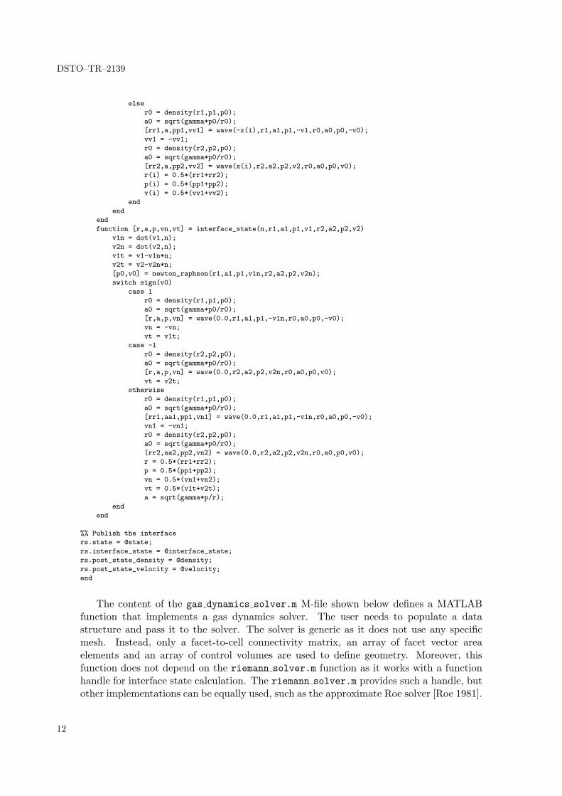
The content of the gas dynamics solver.m M-file shown below defines a MATLABfunction that implements a gas dynamics solver. The user needs to populate a datastructure and pass it to the solver. The solver is generic as it does not use any specificmesh. Instead, only a facet-to-cell connectivity matrix, an array of facet vector areaelements and an array of control volumes are used to define geometry. Moreover, thisfunction does not depend on the riemann solver.m function as it works with a functionhandle for interface state calculation. The riemann solver.m provides such a handle, butother implementations can be equally used, such as the approximate Roe solver [Roe 1981].

12

DSTO–TR–2139

function gds = gas_dynamics_solver

% gds = gas_dynamics_solver

%

% Gas dynamics solver.

%

% Function handles:

%

% model = gds.initialise(model)

%

% Validates the model structure, allocates auxiliary fields and populates

% the conserved variables.

%

% model = gds.update_rates(model)

%

% Calculates the interface states from the current physical variables and

% updates the rates of the conserved variables.

%

% model = gds.update_states(model)

%

% Updates the physical variables from the conserved variables.

% Should be always called after advancing the time step and appying

% boundary conditions that must affect the conserved variables only.

%

% The model structure must contain the following fields:

%

% model.gamma - polytropic index

% model.state - interface state sampling handle

% model.fc - facet-to-cell connectivity matrix

% model.ds - vector area elements

% model.dv - volume elements

% model.r - density

% model.p - pressure

% model.v - velocity

%

% The following auxiliary fields will be allocated:

%

% model.gamma1 - model.gamma - 1

% model.da - facet area elements

% model.n - facet unit normal vectors

% model.a - sound speed

% model.e - total energy

% model.u - momentum

% model.r_rate - density rate

% model.e_rate - total energy rate

% model.u_rate - momentum rate

% model.ir - interface density

% model.ip - interface pressure

% model.ia - interface sound speed

% model.ivn - interface normal component of velocity

%

% Examples:

%

% *** Sod’s shock tube ***

%

% model.gamma = 1.4; rs = riemann_solver(model.gamma);

% model.state = rs.interface_state; gds = gas_dynamics_solver;

% N = 200; L = 1.0; dx = L/N; x = -dx/2:dx:1+dx/2;

% model.dv = dx*ones(N+2,1); model.ds = ones(N+1,1);

% model.fc = [1:N+1;2:N+2].’; model.r = zeros(N+2,1);

% model.p = zeros(N+2,1); model.v = zeros(N+2,1);

% boundary_cells = [2,N+1]; ghost_cells = [1,N+2];

% for i = 1:N+2

% if x(i) < L/2

% model.r(i) = 1.0; model.p(i) = 1.0;

% else

% model.r(i) = 0.125; model.p(i) = 0.1;

% end

13

DSTO–TR–2139

% end

% model = gds.initialise(model);

% t = 0; tf = 0.25;

% while t < tf

% model = gds.update_rates(model);

% dt = dx/max(model.ia+abs(model.ivn));

% dt = min(dt,tf-t); t = t+dt;

% model.r = model.r+model.r_rate*dt;

% model.e = model.e+model.e_rate*dt;

% model.u = model.u+model.u_rate*dt;

% model.r(ghost_cells) = model.r(boundary_cells);

% model.e(ghost_cells) = model.e(boundary_cells);

% model.u(ghost_cells) = model.u(boundary_cells);

% model = gds.update_states(model);

% subplot(3,1,1);

% plot(x(2:end-1),model.r(2:end-1),’.’);

% title(sprintf(’Density at t = %g’,t));

% subplot(3,1,2);

% plot(x(2:end-1),model.p(2:end-1),’.’);

% title(sprintf(’Pressure at t = %g’,t));

% subplot(3,1,3);

% plot(x(2:end-1),model.v(2:end-1),’.’);

% title(sprintf(’Velocity at t = %g’,t));

% drawnow;

% end

%

% See also riemann_solver

%

% Copyright 2007-2008 Defence Science and Technology Organisation

%% Define function handles

function model = initialise(model)

% Check required fields

if ~isfield(model,’gamma’)

error(’Undefined polytropic index: model.gamma’);

end

if ~isfield(model,’state’)

error(’Undefined interface state sampling handle: model.state’);

end

if ~isa(model.state,’function_handle’)

error(’Field model.state must be a function handle’);

end

if ~isfield(model,’fc’)

error(’Undefined facet-to-cell connectivity matrix: model.fc’);

end

if ~isfield(model,’ds’)

error(’Undefined vector area elements: model.ds’);

end

if ~isfield(model,’dv’)

error(’Undefined volume elements: model.dv’);

end

if ~isfield(model,’r’)

error(’Undefined density: model.r’);

end

if ~isfield(model,’p’)

error(’Undefined pressure: model.p’);

end

if ~isfield(model,’v’)

error(’Undefined velocity: model.v’);

end

% Check consistency

if size(model.ds,2) ~= size(model.v,2)

error(’Unequal number of columns of model.ds and model.v’);

end

model.DIM = size(model.v,2);

if model.DIM < 1 || model.DIM > 3

error(’Invalid space dimension: %d’,model.DIM);

14

DSTO–TR–2139

end

if size(model.fc,2) ~= 2

error(’Connectivity matrix must have two columns’);

end

if size(model.dv,2) ~= 1

error(’Control volumes must form a column vector’);

end

if size(model.r,2) ~= 1

error(’Density field must be a column vector’);

end

if size(model.p,2) ~= 1

error(’Pressure field must be a column vector’);

end

if size(model.dv,1) ~= size(model.r,1)

error(’Unequal number of rows of model.dv and model.r’);

end

if size(model.dv,1) ~= size(model.p,1)

error(’Unequal number of rows of model.dv and model.p’);

end

if size(model.dv,1) ~= size(model.v,1)

error(’Unequal number of rows of model.dv and model.v’);

end

% Initialise

model.gamma1 = model.gamma-1.0;

model.da = sqrt(dot(model.ds,model.ds,2));

model.n(:,1) = model.ds(:,1)./model.da;

if model.DIM > 1


if model.DIM > 2


end

end

model.a = zeros(size(model.r));

model.e = zeros(size(model.p));

model.u = zeros(size(model.v));

model.r_rate = zeros(size(model.r));

model.e_rate = zeros(size(model.e));

model.u_rate = zeros(size(model.u));

model.ir = zeros(size(model.ds,1),1);

model.ip = zeros(size(model.ds,1),1);

model.ia = zeros(size(model.ds,1),1);

model.ivn = zeros(size(model.ds,1),1);

model.a = sqrt(model.gamma*model.p./model.r);

model.u(:,1) = model.r.*model.v(:,1);

if model.DIM > 1


if model.DIM > 2


end

end

model.e = model.p/model.gamma1+0.5*dot(model.u,model.v,2);

end

function model = update_rates(model)

model.r_rate = zeros(size(model.r_rate));

model.e_rate = zeros(size(model.e_rate));

model.u_rate = zeros(size(model.u_rate));

for k = 1:size(model.fc,1)

i1 = model.fc(k,1);

i2 = model.fc(k,2);

[r,a,p,vn,vt] = model.state(model.n(k,:),...

model.r(i1),model.a(i1),model.p(i1),model.v(i1,:),...

model.r(i2),model.a(i2),model.p(i2),model.v(i2,:));

model.ir(k) = r;

model.ia(k) = a;

model.ip(k) = p;

model.ivn(k) = vn;

v = vt+vn*model.n(k,:);

15

DSTO–TR–2139

r_flux = r*vn*model.da(k);

e_flux = r_flux*(a*a/model.gamma1+0.5*dot(v,v,2));

u_flux = r_flux*v+p*model.ds(k,:);

model.r_rate(i1) = model.r_rate(i1)-r_flux;

model.r_rate(i2) = model.r_rate(i2)+r_flux;

model.e_rate(i1) = model.e_rate(i1)-e_flux;

model.e_rate(i2) = model.e_rate(i2)+e_flux;

model.u_rate(i1,:) = model.u_rate(i1,:)-u_flux;

model.u_rate(i2,:) = model.u_rate(i2,:)+u_flux;

end

model.r_rate = model.r_rate./model.dv;

model.e_rate = model.e_rate./model.dv;

model.u_rate(:,1) = model.u_rate(:,1)./model.dv;

if model.DIM > 1


if model.DIM > 2


end

end

end

function model = update_states(model)

model.v(:,1) = model.u(:,1)./model.r;

if model.DIM > 1


if model.DIM > 2


end

end

model.p = model.gamma1*(model.e-0.5*dot(model.u,model.v,2));

model.a = sqrt(model.gamma*model.p./model.r);

end

%% Publish the interface

gds.initialise = @initialise;

gds.update_rates = @update_rates;

gds.update_states = @update_states;

end

6 Usage examples

6.1 Sod’s shock tube

The exact similarity solution to Sod’s shock tube [Sod 1978] specified by the followinginitial piecewise-constant state of gas

(ρ, p, v) =

{(1.0, 1.0, 0.0) (x < 0)

(0.125, 0.1, 0.0) (x > 0)(40)

provides a useful benchmark for gas dynamics solvers.

The following MATLAB script simulates the benchmark problem of ideal polytropicgas with specific heat ratio γ = 1.4 on a uniform mesh consisting of 400 control cells. Thenumerical results are displayed in Figure 2. It is seen that the numerical solution and theexact benchmark solution are in good agreement. Note that, due to numerical viscosity,the contact discontinuity is smeared out to some extent whereas the shock front positionis captured quite accurately.

16

DSTO–TR–2139

(i) Pressure. (ii) Density.

(iii) Velocity. (iv) Internal energy.

Figure 2: Gas state in Sod’s shock tube at time t = 0.25.

%% Sod’s shock tube simulation

x1 = -0.5; r1 = 1.0; p1 = 1.0; v1 = 0.0;

x2 = 0.5; r2 = 0.125; p2 = 0.1; v2 = 0.0;

tf = 0.25; NX = 400;

%% Benchmark solution

model.gamma = 1.4; rs = riemann_solver(model.gamma);

model.state = rs.interface_state;

X = linspace(x1,x2,1000); [R,P,V] = rs.state(X/tf,r1,p1,v1,r2,p2,v2);

%% Generate a uniform mesh

dx = (x2-x1)/NX; x = (x1-dx/2:dx:x2+dx/2).’;

model.fc = [1:NX+1;2:NX+2].’; model.ds = ones(NX+1,1);

model.dv = dx*ones(NX+2,1); B = [2,NX+1]; G = [1,NX+2]; I = 2:NX;

%% Run simulation

disp(’*** Sod’’s shock tube ***’);

t = 0.0;

[model.r,model.p,model.v] = rs.state(x/t,r1,p1,v1,r2,p2,v2);

model.v = zeros(NX+2,1); gds = gas_dynamics_solver;

model = gds.initialise(model);

while t < tf

model = gds.update_rates(model);

dt = dx/max(model.ia+abs(model.ivn));

17

DSTO–TR–2139

dt = min(dt,tf-t); t = t+dt; disp(sprintf(’t = %g’,t));

model.r = model.r+model.r_rate*dt;

model.e = model.e+model.e_rate*dt;

model.u = model.u+model.u_rate*dt;

model.r(G) = model.r(B);

model.e(G) = model.e(B);

model.u(G) = -model.u(B);

model = gds.update_states(model);

end

%% Plot the final state

plot(X,R,’r-’,x,model.r,’b.’); grid on;

axis([x1,x2,0,1.2]); legend(’exact’,’numerical’,’Location’,’Best’);

print -dpng sod_shock_tube_density;

plot(X,P./R/model.gamma1,’r-’,x,model.p./model.r/model.gamma1,’b.’); grid on;

axis([x1,x2,1.0,3.0]); legend(’exact’,’numerical’,’Location’,’Best’);

print -dpng sod_shock_tube_energy;

plot(X,P,’r-’,x,model.p,’b.’); grid on;


print -dpng sod_shock_tube_pressure;

plot(X,V,’r-’,x,model.v,’b.’); grid on;


print -dpng sod_shock_tube_velocity;

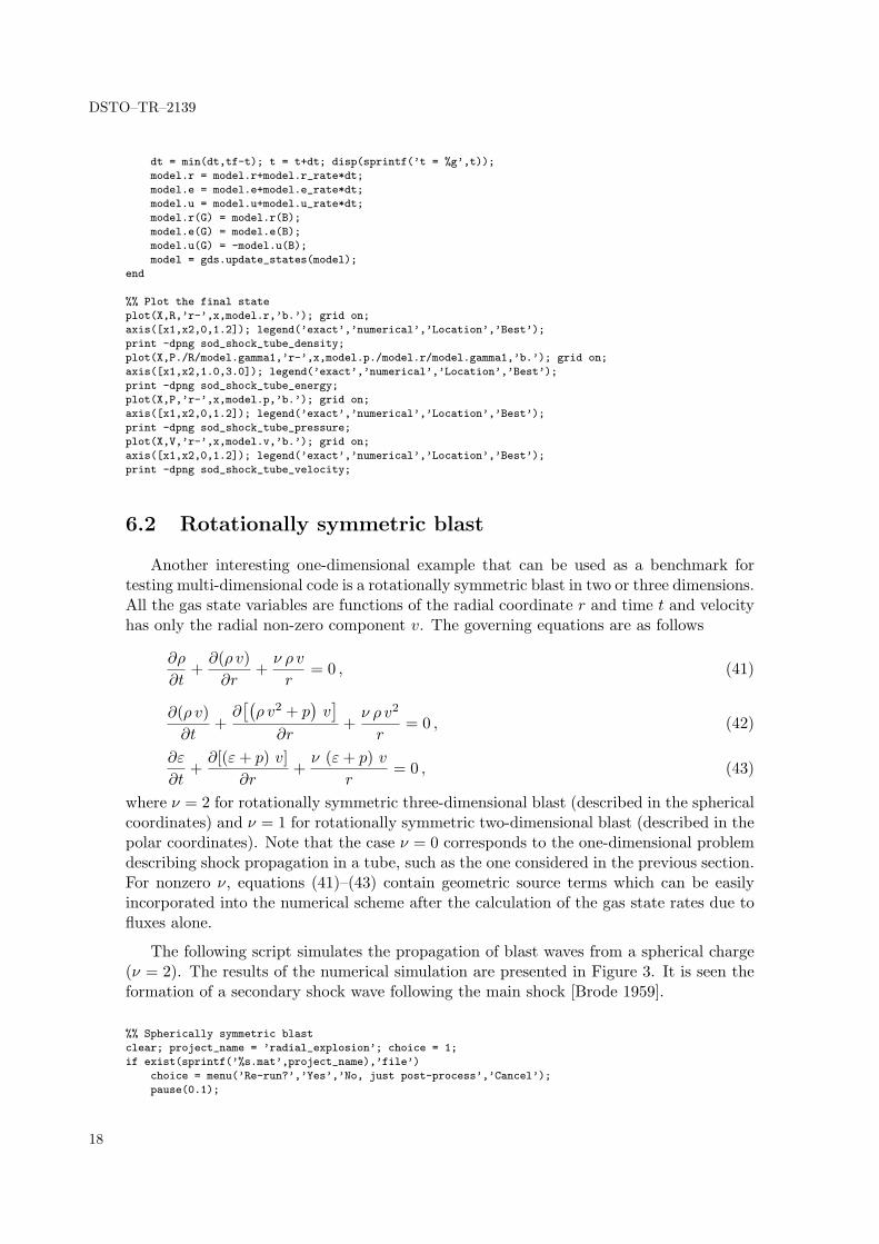
6.2 Rotationally symmetric blast

Another interesting one-dimensional example that can be used as a benchmark fortesting multi-dimensional code is a rotationally symmetric blast in two or three dimensions.All the gas state variables are functions of the radial coordinate r and time t and velocityhas only the radial non-zero component v. The governing equations are as follows

∂ρ

∂t+∂(ρ v)∂r

+ν ρ v

r= 0 , (41)

∂(ρ v)∂t

+∂[(ρ v2 + p

)v]

∂r+ν ρ v2

r= 0 , (42)

∂ε

∂t+∂[(ε+ p) v]

∂r+ν (ε+ p) v

r= 0 , (43)

where ν = 2 for rotationally symmetric three-dimensional blast (described in the sphericalcoordinates) and ν = 1 for rotationally symmetric two-dimensional blast (described in thepolar coordinates). Note that the case ν = 0 corresponds to the one-dimensional problemdescribing shock propagation in a tube, such as the one considered in the previous section.For nonzero ν, equations (41)–(43) contain geometric source terms which can be easilyincorporated into the numerical scheme after the calculation of the gas state rates due tofluxes alone.

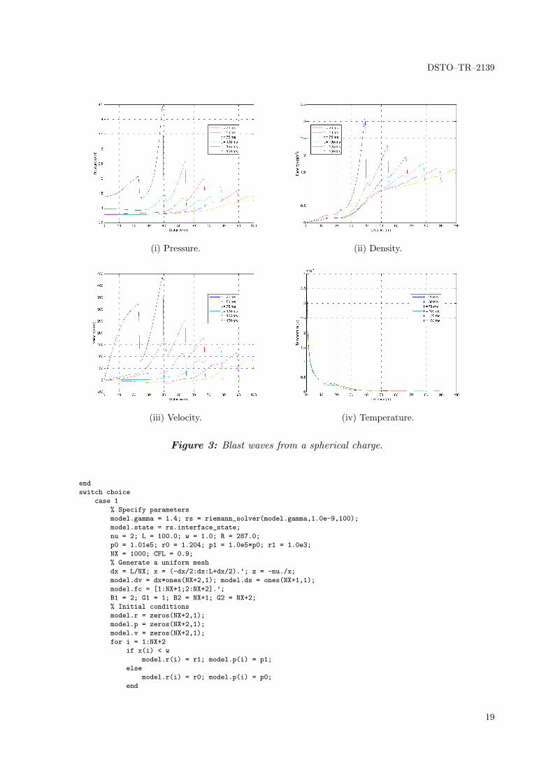
The following script simulates the propagation of blast waves from a spherical charge(ν = 2). The results of the numerical simulation are presented in Figure 3. It is seen theformation of a secondary shock wave following the main shock [Brode 1959].

%% Spherically symmetric blast

clear; project_name = ’radial_explosion’; choice = 1;

if exist(sprintf(’%s.mat’,project_name),’file’)

choice = menu(’Re-run?’,’Yes’,’No, just post-process’,’Cancel’);

pause(0.1);

18

DSTO–TR–2139

(i) Pressure. (ii) Density.

(iii) Velocity. (iv) Temperature.

Figure 3: Blast waves from a spherical charge.

end

switch choice

case 1

% Specify parameters

model.gamma = 1.4; rs = riemann_solver(model.gamma,1.0e-9,100);

model.state = rs.interface_state;

nu = 2; L = 100.0; w = 1.0; R = 287.0;

p0 = 1.01e5; r0 = 1.204; p1 = 1.0e5*p0; r1 = 1.0e3;

NX = 1000; CFL = 0.9;

% Generate a uniform mesh

dx = L/NX; x = (-dx/2:dx:L+dx/2).’; z = -nu./x;

model.dv = dx*ones(NX+2,1); model.ds = ones(NX+1,1);

model.fc = [1:NX+1;2:NX+2].’;

B1 = 2; G1 = 1; B2 = NX+1; G2 = NX+2;

% Initial conditions

model.r = zeros(NX+2,1);

model.p = zeros(NX+2,1);

model.v = zeros(NX+2,1);

for i = 1:NX+2

if x(i) < w

model.r(i) = r1; model.p(i) = p1;

else

model.r(i) = r0; model.p(i) = p0;

end

19

DSTO–TR–2139

end

% Allocate variables for post-processing

times = [0.025,0.05,0.075,0.1,0.125,0.15]; K = length(times);

pressures = zeros(NX,K);

velocities = zeros(NX,K);

densities = zeros(NX,K);

temperatures = zeros(NX,K);

I = 2:NX+1; x = x(I);

% Run simulation

disp(’*** Spherically symmetric blast ***’);

gs = gas_dynamics_solver; model = gs.initialise(model);

t = 0.0;

for k = 1:K

tf = times(k);

while t < tf

model = gs.update_rates(model);

dt = CFL*dx/max(abs(model.ivn)+model.ia);

dt = min(dt,tf-t); t = t+dt;




model = gs.update_states(model);

model.r_rate = z.*model.u;

model.e_rate = model.r_rate.*(model.e+model.p)./model.r;

model.u_rate = model.r_rate.*model.v;




model.r(G1) = model.r(B1); % reflective BC

model.e(G1) = model.e(B1);

model.u(G1) = -model.u(B1);

model.r(G2) = model.r(B2); % open-end BC

model.e(G2) = model.e(B2);

model.u(G2) = model.u(B2);

model = gs.update_states(model);

plot(x,model.p(I),’k.’);

title(sprintf(’Pressure at t = %g’,t));

drawnow;

end

pressures(:,k) = model.p(I);

velocities(:,k) = model.v(I);

densities(:,k) = model.r(I);

temperatures(:,k) = model.p(I)./model.r(I)/R;

end

save(project_name);

case 2

load(project_name);

otherwise

return;

end

%% Generate images

info = cell(size(times));

for k = 1:K

info{k} = sprintf(’t = %g ms’,1000.0*times(k));

end

figure; plot(x,pressures/p0); grid on;

xlabel(’Distance (m)’); ylabel(’Pressure (atm)’);

legend(info,’Location’,’Best’);

eval(sprintf(’print -dpng %s_pressure’,project_name));

figure; plot(x,velocities); grid on;

xlabel(’Distance (m)’); ylabel(’Velocity (m/s)’);


eval(sprintf(’print -dpng %s_velocity’,project_name));

figure; plot(x,densities); grid on;

xlabel(’Distance (m)’); ylabel(’Density (kg/m^3)’);


eval(sprintf(’print -dpng %s_density’,project_name));

20

DSTO–TR–2139

figure; plot(x,temperatures); grid on;

xlabel(’Distance (m)’); ylabel(’Temperature (K)’);


eval(sprintf(’print -dpng %s_temperature’,project_name));

6.3 Two-dimensional blast propagation

Consider a two-dimensional explosion in air occupying a square domain with a sidelength of 10 m at initial atmospheric pressure of 101 kPa (1 atmosphere) and temperatureof 20◦C. The blast is modelled by a localised region of 10-atmosphere over-pressure andtemperature of 2000◦C.

The following MATLAB script simulates this problem on a uniform mesh. The pressureand temperature fields for increasing times are presented in Figures 4 and 5 respectively.

%% 2D blast propagation in a square domain

project_name = ’blast2d’;

disp(sprintf(’Project name: %s’,project_name));

gds = gas_dynamics_solver;

R = 287.0; Kelvin0 = 273.0;

T0 = Kelvin0+20.0; p0 = 1.01e5; r0 = p0/T0/R;

T1 = Kelvin0+2000.0; p1 = 11*p0; r1 = p1/T1/R;

CFL = 0.5; save_time = 0.002; kmax = 6;

%% Pre-process if necessary

k = 0;

if ~exist(sprintf(’%s%d.mat’,project_name,k),’file’)

% Generate mesh

s.LX = 10.0; s.LY = 10.0; s.NX = 250; s.NY = 250;

s.map = @(ix,iy) sub2ind([s.NX+2,s.NY+2],ix,iy);

dx = s.LX/s.NX; dy = s.LY/s.NY; s.dx = min([dx,dy]);

s.x = -dx/2:dx:s.LX+dx/2; s.y = -dy/2:dy:s.LY+dy/2;

NC = (s.NX+2)*(s.NY+2); NF = (s.NX+1)*s.NY+s.NX*(s.NY+1);

disp(sprintf(’%d facets, %d cells’,NF,NC-4));

s.dv = (dx*dy)*ones(NC,1); s.fc = zeros(NF,2); s.ds = zeros(NF,2);

s.BE = zeros(s.NY,1); s.GE = zeros(s.NY,1); % east BC

s.BW = zeros(s.NY,1); s.GW = zeros(s.NY,1); % west BC

s.BS = zeros(s.NX,1); s.GS = zeros(s.NX,1); % south BC

s.BN = zeros(s.NX,1); s.GN = zeros(s.NX,1); % north BC

i = 0; % facet index

for ix = 1:s.NX+1

for iy = 2:s.NY+1

i = i+1; s.ds(i,:) = [dy,0];

s.fc(i,1) = s.map(ix,iy);

s.fc(i,2) = s.map(ix+1,iy);

end

end

for iy = 1:s.NY+1

for ix = 2:s.NX+1

i = i+1; s.ds(i,:) = [0,dx];

s.fc(i,1) = s.map(ix,iy);

s.fc(i,2) = s.map(ix,iy+1);

end

end

for iy = 2:s.NY+1

s.BE(iy-1) = s.map(2,iy); s.GE(iy-1) = s.map(1,iy);

s.BW(iy-1) = s.map(s.NX+1,iy); s.GW(iy-1) = s.map(s.NX+2,iy);

end

for ix = 2:s.NX+1

s.BS(ix-1) = s.map(ix,2); s.GS(ix-1) = s.map(ix,1);

s.BN(ix-1) = s.map(ix,s.NY+1); s.GN(ix-1) = s.map(ix,s.NY+2);

end

21

DSTO–TR–2139


xa = 7.0; ya = 8.0; a = 0.5; b = 100.0;

density = @(x,y)...

0.5*((r1+r0)+(r1-r0)*tanh(b*(a-sqrt((x-xa)^2+(y-ya)^2))));

pressure = @(x,y)...

0.5*((p1+p0)+(p1-p0)*tanh(b*(a-sqrt((x-xa)^2+(y-ya)^2))));

s.r = zeros(NC,1); s.p = zeros(NC,1); s.v = zeros(NC,2);

for ix = 1:s.NX+2

for iy = 1:s.NY+2

i = s.map(ix,iy);

s.r(i) = density(s.x(ix),s.y(iy));

s.p(i) = pressure(s.x(ix),s.y(iy));

end

end

% Specify Riemann solver

s.gamma = 1.4; rs = riemann_solver(s.gamma);

s.state = rs.interface_state; s.t = 0.0; s = gds.initialise(s);

eval(sprintf(’save %s%d -struct s’,project_name,k));

end

%% Find the latest restart file

while exist(sprintf(’%s%d.mat’,project_name,k),’file’)

k = k+1;

end

k = k-1;

%% Load start/restart file

s = load(sprintf(’%s%d’,project_name,k));

while k < kmax

elapsed_time = cputime;

k = k+1;

tf = s.t + save_time;

while s.t < tf

s = gds.update_rates(s);

dt = CFL*s.dx/max(s.ia+abs(s.ivn));

dt = min(dt,tf-s.t); s.t = s.t+dt;

disp(sprintf(’t = %g’,s.t));

s.r = s.r+s.r_rate*dt;

s.e = s.e+s.e_rate*dt;

s.u = s.u+s.u_rate*dt;

% reflective east BC

s.r(s.GE) = s.r(s.BE); s.e(s.GE) = s.e(s.BE);

s.u(s.GE,1) = -s.u(s.BE,1); s.u(s.GE,2) = s.u(s.BE,2);

% reflective west BC

s.r(s.GW) = s.r(s.BW); s.e(s.GW) = s.e(s.BW);

s.u(s.GW,1) = -s.u(s.BW,1); s.u(s.GW,2) = s.u(s.BW,2);

% reflective south BC

s.r(s.GS) = s.r(s.BS); s.e(s.GS) = s.e(s.BS);

s.u(s.GS,1) = s.u(s.BS,1); s.u(s.GS,2) = -s.u(s.BS,2);

% reflective north BC

s.r(s.GN) = s.r(s.BN); s.e(s.GN) = s.e(s.BN);

s.u(s.GN,1) = s.u(s.BN,1); s.u(s.GN,2) = -s.u(s.BN,2);

% synchronise physical variables

s = gds.update_states(s);

end

elapsed_time = cputime-elapsed_time;

disp(sprintf(’CPU time: %g secs / %g mins / %g hours’,...

elapsed_time,elapsed_time/60,elapsed_time/3600));


end

%% Post process

disp(’Generating PNG images...’);

set(clf,’Renderer’,’ZBuffer’);

k = 0;



22

DSTO–TR–2139

[x,y] = ndgrid(s.x,s.y); z = zeros(size(x));

for ix = 2:s.NX+1

for iy = 2:s.NY+1

i = s.map(ix,iy);

z(ix,iy) = s.p(i)/1000;

end

end

surf(x(2:end-1,2:end-2),y(2:end-1,2:end-2),z(2:end-1,2:end-2));

title(sprintf(’Pressure (kPa) at time t = %g ms’,1000*s.t));

axis([0,s.LX,0,s.LY,0,p1/2000]); shading interp;

eval(sprintf(’print -dpng %s%d_pressure’,project_name,k));

for ix = 2:s.NX+1

for iy = 2:s.NY+1

i = s.map(ix,iy);

z(ix,iy) = s.p(i)/s.r(i)/R;

end

end

surf(x(2:end-1,2:end-2),y(2:end-1,2:end-2),z(2:end-1,2:end-2));

title(sprintf(’Temperature (K) at time t = %g ms’,1000*s.t));

axis([0,s.LX,0,s.LY,0,T1]); shading interp;

eval(sprintf(’print -dpng %s%d_temperature’,project_name,k));

k = k+1;

end

23

DSTO–TR–2139

(i) t = 2 ms. (ii) t = 4 ms.

(iii) t = 6 ms. (iv) t = 8 ms.

(v) t = 10 ms. (vi) t = 12 ms.

Figure 4: Two-dimensional blast propagation; pressure field surfaces.

24

DSTO–TR–2139

(i) t = 2 ms. (ii) t = 4 ms.

(iii) t = 6 ms. (iv) t = 8 ms.

(v) t = 10 ms. (vi) t = 12 ms.

Figure 5: Two-dimensional blast propagation; temperature field surfaces.

25

DSTO–TR–2139

6.4 Three-dimensional blast propagation

Consider three-dimensional explosion in air occupying a block with dimensions 25by 10 by 20 m with the initial conditions similar to the previous section. The charge ispositioned at a corner of the block. Both reflective and non-reflective boundary conditionsare imposed on the walls of the block to model blast propagation in a street canyon underthe assumption that the charge is positioned at the ground level at the centre line of thestreet.

The following MATLAB script simulates this problem on a uniform mesh. The pressureand temperature fields for increasing times are presented in Figures 6 and 7. It is clearlyseen the formation of a secondary shock wave.

%% 3D blast propagation in a street canyon

project_name = ’blast3d’;

disp(sprintf(’Project name: %s’,project_name));

gds = gas_dynamics_solver;

R = 287.0; Kelvin0 = 273.0;

T0 = Kelvin0+20.0; p0 = 1.01e5; r0 = p0/T0/R;

T1 = Kelvin0+2000.0; p1 = 11*p0; r1 = p1/T1/R;

CFL = 0.5; save_time = 0.005; kmax = 6;

%% Pre-process if necessary

k = 0;

if ~exist(sprintf(’%s%d.mat’,project_name,k),’file’)

% Generate mesh

s.LX = 25.0; s.LY = 10.0; s.LZ = 20.0;

s.NX = 100; s.NY = 40; s.NZ = 80;

dx = s.LX/s.NX; dy = s.LY/s.NY; dz = s.LZ/s.NZ; s.dx = min([dx,dy,dz]);

s.x = -dx/2:dx:s.LX+dx/2; s.y = -dy/2:dy:s.LY+dy/2; s.z = -dz/2:dz:s.LZ+dz/2;

NC = (s.NX+2)*(s.NY+2)*(s.NZ+2);

NF = (s.NX+1)*s.NY*s.NZ+s.NX*(s.NY+1)*s.NZ+s.NX*s.NY*(s.NZ+1);

disp(sprintf(’%d facets, %d cells’,NF,NC-8));

s.dv = (dx*dy*dz)*ones(NC,1); s.fc = zeros(NF,2); s.ds = zeros(NF,3);

s.BE = zeros(s.NY*s.NZ,1); s.GE = zeros(s.NY*s.NZ,1); % east BC

s.BW = zeros(s.NY*s.NZ,1); s.GW = zeros(s.NY*s.NZ,1); % west BC

s.BS = zeros(s.NX*s.NZ,1); s.GS = zeros(s.NX*s.NZ,1); % south BC

s.BN = zeros(s.NX*s.NZ,1); s.GN = zeros(s.NX*s.NZ,1); % north BC

s.BB = zeros(s.NX*s.NY,1); s.GB = zeros(s.NX*s.NY,1); % bottom BC

s.BT = zeros(s.NX*s.NY,1); s.GT = zeros(s.NX*s.NY,1); % top BC

s.map = @(ix,iy,iz) sub2ind([s.NX+2,s.NY+2,s.NZ+2],ix,iy,iz);

i = 0; % facet index

for ix = 1:s.NX+1

for iy = 2:s.NY+1

for iz = 2:s.NZ+1

i = i+1; s.ds(i,:) = [dy*dz,0,0];

s.fc(i,1) = s.map(ix,iy,iz);

s.fc(i,2) = s.map(ix+1,iy,iz);

end

end

end

for ix = 2:s.NX+1

for iy = 1:s.NY+1

for iz = 2:s.NZ+1

i = i+1; s.ds(i,:) = [0,dx*dz,0];


s.fc(i,2) = s.map(ix,iy+1,iz);

end

end

end

for ix = 2:s.NX+1

for iy = 2:s.NY+1

26

DSTO–TR–2139

for iz = 1:s.NZ+1

i = i+1; s.ds(i,:) = [0,0,dx*dy];


s.fc(i,2) = s.map(ix,iy,iz+1);

end

end

end

for iy = 2:s.NY+1

for iz = 2:s.NZ+1

i = sub2ind([s.NY,s.NZ],iy-1,iz-1);

s.BE(i) = s.map(2,iy,iz); s.GE(i) = s.map(1,iy,iz);

s.BW(i) = s.map(s.NX+1,iy,iz); s.GW(i) = s.map(s.NX+2,iy,iz);

end

end

for ix = 2:s.NX+1

for iz = 2:s.NZ+1

i = sub2ind([s.NX,s.NZ],ix-1,iz-1);

s.BS(i) = s.map(ix,2,iz); s.GS(i) = s.map(ix,1,iz);

s.BN(i) = s.map(ix,s.NY+1,iz); s.GN(i) = s.map(ix,s.NY+2,iz);

end

end

for ix = 2:s.NX+1

for iy = 2:s.NY+1

i = sub2ind([s.NX,s.NY],ix-1,iy-1);

s.BB(i) = s.map(ix,iy,2); s.GB(i) = s.map(ix,iy,1);

s.BT(i) = s.map(ix,iy,s.NZ+1); s.GT(i) = s.map(ix,iy,s.NZ+2);

end

end


xa = 0.0; ya = 0.0; za = 0.0; a = 5.0; b = 100.0;

density = @(x,y,z)...

0.5*((r1+r0)+(r1-r0)*tanh(...

b*(a-sqrt((x-xa)^2+(y-ya)^2+(z-za)^2))));

pressure = @(x,y,z)...

0.5*((p1+p0)+(p1-p0)*tanh(...

b*(a-sqrt((x-xa)^2+(y-ya)^2+(z-za)^2))));

s.r = zeros(NC,1); s.p = zeros(NC,1); s.v = zeros(NC,3);

for ix = 1:s.NX+2

for iy = 1:s.NY+2

for iz = 1:s.NZ+2

i = s.map(ix,iy,iz);

s.r(i) = density(s.x(ix),s.y(iy),s.z(iz));

s.p(i) = pressure(s.x(ix),s.y(iy),s.z(iz));

end

end

end

% Specify Riemann solver

s.gamma = 1.4; rs = riemann_solver(s.gamma);

s.state = rs.interface_state; s.t = 0.0; s = gds.initialise(s);


end

%% Find the latest restart file


k = k+1;

end

k = k-1;

%% Load start/restart file


while k < kmax

elapsed_time = cputime;

k = k+1;

tf = s.t + save_time;

while s.t < tf

s = gds.update_rates(s);

dt = CFL*s.dx/max(s.ia+abs(s.ivn));

27

DSTO–TR–2139

dt = min(dt,tf-s.t); s.t = s.t+dt;

disp(sprintf(’t = %g’,s.t));

s.r = s.r+s.r_rate*dt;

s.e = s.e+s.e_rate*dt;

s.u = s.u+s.u_rate*dt;

% reflective east BC (symmetry plane)

s.r(s.GE) = s.r(s.BE); s.e(s.GE) = s.e(s.BE);

s.u(s.GE,1) = -s.u(s.BE,1); s.u(s.GE,2) = s.u(s.BE,2);

s.u(s.GE,3) = s.u(s.BE,3);

% non-reflective west BC

s.r(s.GW) = s.r(s.BW); s.e(s.GW) = s.e(s.BW);

s.u(s.GW,1) = s.u(s.BW,1); s.u(s.GW,2) = s.u(s.BW,2);

s.u(s.GW,3) = s.u(s.BW,3);

% reflective south BC (symmetry plane)

s.r(s.GS) = s.r(s.BS); s.e(s.GS) = s.e(s.BS);

s.u(s.GS,1) = s.u(s.BS,1); s.u(s.GS,2) = -s.u(s.BS,2);

s.u(s.GS,3) = s.u(s.BS,3);

% reflective north BC

s.r(s.GN) = s.r(s.BN); s.e(s.GN) = s.e(s.BN);

s.u(s.GN,1) = s.u(s.BN,1); s.u(s.GN,2) = -s.u(s.BN,2);

s.u(s.GN,3) = s.u(s.BN,3);

% reflective bottom BC

s.r(s.GB) = s.r(s.BB); s.e(s.GB) = s.e(s.BB);

s.u(s.GB,1) = s.u(s.BB,1); s.u(s.GB,2) = s.u(s.BB,2);

s.u(s.GB,3) = -s.u(s.BB,3);

% non-reflective top BC

s.r(s.GT) = s.r(s.BT); s.e(s.GT) = s.e(s.BT);

s.u(s.GT,1) = s.u(s.BT,1); s.u(s.GT,2) = s.u(s.BT,2);

s.u(s.GT,3) = s.u(s.BT,3);

% synchronise physical variables

s = gds.update_states(s);

end

elapsed_time = cputime-elapsed_time;

disp(sprintf(’CPU time: %g secs / %g mins / %g hours’,...

elapsed_time,elapsed_time/60,elapsed_time/3600));


end

%% Post process

disp(’Generating PNG images...’);

set(clf,’Renderer’,’ZBuffer’);

k = 0;



sx = s.x(s.NX+1); sy = [s.y(2),s.y(s.NY+1)]; sz = s.z(2);

[x,y,z] = ndgrid(s.x,s.y,s.z); w = zeros(size(x));

for ix = 2:s.NX+1

for iy = 2:s.NY+1

for iz = 2:s.NZ+1


w(ix,iy,iz) = s.p(i)/1000;

end

end

end

slice(...

y(2:end-1,2:end-1,2:end-1),...

x(2:end-1,2:end-1,2:end-1),...

z(2:end-1,2:end-1,2:end-1),...

w(2:end-1,2:end-1,2:end-1),...

sy,sx,sz);

daspect([1,1,1]); axis equal; colorbar;

title(sprintf(’Pressure (kPa) at time t = %g ms’,1000*s.t));

eval(sprintf(’print -dpng %s%d_pressure’,project_name,k));

for ix = 2:s.NX+1

for iy = 2:s.NY+1

for iz = 2:s.NZ+1


28

DSTO–TR–2139

w(ix,iy,iz) = s.p(i)/s.r(i)/R;

end

end

end

slice(...

y(2:end-1,2:end-1,2:end-1),...

x(2:end-1,2:end-1,2:end-1),...

z(2:end-1,2:end-1,2:end-1),...

w(2:end-1,2:end-1,2:end-1),...

sy,sx,sz);

daspect([1,1,1]); axis equal; colorbar;

title(sprintf(’Temperature (K) at time t = %g ms’,1000*s.t));

eval(sprintf(’print -dpng %s%d_temperature’,project_name,k));

k = k+1;

end

29

DSTO–TR–2139

(i) t = 5 ms. (ii) t = 10 ms.

(iii) t = 15 ms. (iv) t = 20 ms.

(v) t = 25 ms. (vi) t = 30 ms.

Figure 6: Three-dimensional blast propagation; pressure field slices.

30

DSTO–TR–2139

(i) t = 5 ms. (ii) t = 10 ms.

(iii) t = 15 ms. (iv) t = 20 ms.

(v) t = 25 ms. (vi) t = 30 ms.

Figure 7: Three-dimensional blast propagation; temperature field slices.

31

DSTO–TR–2139

7 Conclusion

The two reusable M-files constituting a Gas Dynamics Toolbox for MATLAB are suffi-cient for simulation of multi-dimensional problems for blast propagation. The comparisonwith the benchmark solution and the results of numerical simulation demonstrate that thecode provides a reasonable solution which can be used for estimation of the peak pressureand impulse of shock waves.

It is worthwhile noting that the described numerical scheme is an implementation ofthe Finite Volume Method which, in turn, is a particular realisation of the Finite Ele-ment Method when both the shape and weighting functions coincide with the character-istic functions of cells ωi. The Finite Volume Method provides a conservative numericalscheme whose solution exhibits highly desirable properties of conservation of total mass,momentum and energy. Though the described first-order accurate Godunov-type solveris susceptible to numerical diffusion on coarse meshes, the total quantities such as thetotal load on part of a wall (e.g. windows and doors of a building) can be estimated quitereliably due to the conservativeness of the scheme.

References

Brode, H. L. (1959) Blast wave from a spherical charge, J. Phys. Fluids 2(2), 217–229.

Courant, R. & Friedrichs, K. O. (1948) Supersonic Flow and Shock Waves, Interscience,London.

Danaila, I., Joly, P., Kaber, S. M. & Postel, M. (2007) Introduction to Scientific Comput-ing: Twelve Computational Projects Solved with MATLAB, Springer, New York.

Diestel, R. (2005) Graph Theory, 3rd edn, Springer, Berlin.

Gilat, A. (2008) MATLAB R©: An Introduction with Applications, Wiley, New York.

Godunov, S. K. (1959) A difference scheme for numerical computation of discontinuoussolutions of hydrodynamic equations, Math. Sbornik 47(3), 271–306. In Russian.

Godunov, S. K. (1999) Reminiscences about difference schemes, J. Comp. Phys. 153(1), 6–25.

Gottlieb, J. J. & Groth, C. P. T. (1988) Assessment of Riemann solvers for unsteadyone-dimensional inviscid flows of perfect gases, J. Comp. Phys. 78(2), 437–458.

Holt, M. (1977) Numerical Methods in Fluid Dynamics, Springer, Berlin.

Klee, H. (2007) Simulation of Dynamic Systems with MATLAB R©and Simulink R©, CRCPress, Boca Raton, FL.

Oran, E. S. & Boris, J. P. (1987) Numerical Simulation of Reactive Flow, Elsevier, NewYork.

32

DSTO–TR–2139

Richtmyer, R. D. & Morton, K. W. (1967) Difference Methods for Initial-Value Problems,2nd edn, Interscience Publishers, New York.

Roe, P. L. (1981) Approximate Riemann solvers, parameter vectors, and differenceschemes, J. Comp. Phys. 43(2), 357–372.

Sod, G. A. (1978) A survey of several finite difference methods for systems of nonlinearhyperbolic conservation laws, J. Comp. Phys. 27(1), 1–31.

Toro, E. F. (1999) Riemann Solvers and Numerical Methods for Fluid Dynamics: A Prac-tical Introduction, 2nd edn, Springer, Berlin.

van Leer, B. (1979) Towards the ultimate conservative difference scheme. V. A second-order sequel to Godunov’s method, J. Comp. Phys. 32(1), 101–136.

33

Page classification:

DEFENCE SCIENCE AND TECHNOLOGY ORGANISATIONDOCUMENT CONTROL DATA

1. CAVEAT/PRIVACY MARKING

2. TITLE

Solving multi-dimensional problems of gas dy-namics using MATLAB R©

3. SECURITY CLASSIFICATION

Document (U)Title (U)Abstract (U)

4. AUTHOR

L. K. Antanovskii

5. CORPORATE AUTHOR

Defence Science and Technology OrganisationPO Box 1500Edinburgh, South Australia 5111, Australia

6a. DSTO NUMBER

DSTO–TR–21396b. AR NUMBER

014-2046c. TYPE OF REPORT

Technical Report7. DOCUMENT DATE

June, 20088. FILE NUMBER

2008/1023518/19. TASK NUMBER

NS 07/00210. SPONSOR 11. No OF PAGES

3312. No OF REFS

1613. URL OF ELECTRONIC VERSION

http://www.dsto.defence.gov.au/corporate/reports/DSTO–TR–2139.pdf

14. RELEASE AUTHORITY

Chief, Weapons Systems Division

15. SECONDARY RELEASE STATEMENT OF THIS DOCUMENT

Approved For Public ReleaseOVERSEAS ENQUIRIES OUTSIDE STATED LIMITATIONS SHOULD BE REFERRED THROUGH DOCUMENT EXCHANGE, PO BOX 1500,EDINBURGH, SOUTH AUSTRALIA 5111

16. DELIBERATE ANNOUNCEMENT

No Limitations17. CITATION IN OTHER DOCUMENTS

No Limitations18. DSTO RESEARCH LIBRARY THESAURUS

Science SimulationPhysics Computational fluid dynamics19. ABSTRACT

This report describes an implementation of a Godunov-type solver for gas dynamics equations inMATLAB R©. The main attention is paid to providing a generic code that can be easily adapted toparticular problems in one, two or three dimensions. This is achieved by employing a cell connectivitymatrix thus allowing one to use various structured and unstructured meshes without modification ofthe core solver. The code has been thoroughly tested for MATLAB Version 7.6 (Release 2008a).

Page classification:

solving multi-dimensional problems of gas …tr{2139 solving multi-dimensional problems of gas...

Documents