solving differential equations with genetic programminglagaris/papers/degen.pdf · genet program...

Genet Program Evolvable Mach (2006) 7:33–54DOI 10.1007/s10710-006-7009-y

Solving differential equations with genetic programming

I. G. Tsoulos · I. E. Lagaris

Received: 7 February 2005 / Revised: 7 November 2005C© Springer Science + Business Media, LLC 2006

Abstract A novel method for solving ordinary and partial differential equations, basedon grammatical evolution is presented. The method forms generations of trial solutionsexpressed in an analytical closed form. Several examples are worked out and in most casesthe exact solution is recovered. When the solution cannot be expressed in a closed analyticalform then our method produces an approximation with a controlled level of accuracy. Wereport results on several problems to illustrate the potential of this approach.

Keywords Grammatical evolution . Genetic programming . Differential equations .

Evolutionary modeling

1. Introduction

A lot of problems in the fields of physics, chemistry, economics etc. can be expressed interms of ordinary differential equations (ODE’s) and partial differential equations (PDE’s).Weather forecasting, quantum mechanics, wave propagation and stock market dynamicsare some examples. For that reason many methods have been proposed for solving ODE’sand PDE’s such as Runge Kutta, Predictor–Corrector [1], radial basis functions [4] andfeedforward neural networks [5]. Recently, methods based on genetic programming havealso been proposed [6], as well as methods that induce the underlying differential equationfrom experimental data [7, 8]. The technique of genetic programming [2], is an optimizationprocess based on the evolution of a large number of candidate solutions through geneticoperations such as replication, crossover and mutation [14]. In this article we propose a novelmethod based on genetic programming. Our method attempts to solve ODE’s and PDE’s bygenerating solutions in a closed analytical form. Offering closed form analytical solutions isvery helpful and highly desirable. Methods that offer such type of solutions have appeared inthe past. We mention the Galerkin type of methods, methods based on neural networks [5],

Communicated by: Hitoshi Iba

I. G. Tsoulos · I. E. Lagaris (�)Department of Computer Science, University of Ioannina, P.O. Box 1186, Ioannina 45110, Greecee-mail: [email protected]

Springer

34 Genet Program Evolvable Mach (2006) 7:33–54

etc. These methods choose a basis set of functions with adjustable parameters and proceedapproximating the solution by varying these parameters. Our method offers closed formsolutions, however the variety of the basis functions involved is not a priori determined, ratheris constructed dynamically as the solution procedure proceeds and can be of high complexityif required. This last feature is the one that distinguishes our method from others. We have notdealt with the problem of differential equation induction from data. The generation is achievedwith the help of grammatical evolution. We used grammatical evolution instead the “classic”tree based genetic programming, because grammatical evolution can produce programs in anarbitrary language, the genetic operations such as crossover and mutation are faster and alsobecause it is far more convenient to symbolically differentiate mathematical expressions. Thecode production is performed using a mapping process governed by a grammar expressed inBackus Naur Form. Grammatical evolution has been applied successfully to problems suchas symbolic regression [11], discovery of trigonometric identities [12], robot control [15],caching algorithms [16], financial prediction [17] etc. The rest of this article is organizedas follows: in Section 2 we give a brief presentation of grammatical evolution, in Section 3we describe in detail the new algorithm, in Section 4 we present several experiments and inSection 5 we present our conclusions and ideas for further work.

2. Grammatical evolution

Grammatical evolution is an evolutionary algorithm that can produce code in any program-ming language. The algorithm requires as inputs the BNF grammar definition of the targetlanguage and the appropriate fitness function. Chromosomes in grammatical evolution, incontrast to classical genetic programming [2], are not expressed as parse trees, but as vectorsof integers. Each integer denotes a production rule from the BNF grammar. The algorithmstarts from the start symbol of the grammar and gradually creates the program string, byreplacing non terminal symbols with the right hand of the selected production rule. Theselection is performed in two steps:

� We read an element from the chromosome (with value V).� We select the rule according to the scheme

Rule = V mod NR (1)

where NR is the number of rules for the specific non-terminal symbol. The process ofreplacing non terminal symbols with the right hand of production rules is continued untileither a full program has been generated or the end of chromosome has been reached. In thelatter case we can reject the entire chromosome or we can start over (wrapping event) fromthe first element of the chromosome. In our approach we allow at most two wrapping eventsto occur.

In our method we used a small part of the C programming language grammar as we cansee in Fig. 1. The numbers in parentheses denote the sequence number of the correspondingproduction rule to be used in the selection procedure described above.

The symbol S in the grammar denotes the start symbol of the grammar. For example,suppose we have the chromosome x = [16, 3, 7, 4, 10, 28, 24, 1, 2, 4]. In Table 1 we showhow a valid function is produced from x. The resulting function in the above example isf (x) = log(x2). Further details about grammatical evolution can be found in [9, 10, 11, 13].

Springer

Genet Program Evolvable Mach (2006) 7:33–54 35

Fig. 1 The grammar of theproposed method

Table 1 Example of program construction

String Chromosome Operation

<expr> 16, 3, 7, 4, 10, 28, 24, 1,2,4 16 mod 7 = 2<func>(<expr>) 3, 7, 4, 10, 28, 24, 1, 2, 4 3 mod 4 = 3log(<expr>) 7, 4, 10, 28, 24, 1, 2, 4 7 mod 7 = 0log(<expr><op><expr>) 4, 10, 28, 24, 1, 2, 4 4 mod 7 = 4log(x<op><expr>) 10, 28, 24, 1, 2, 4 10 mod 4 = 2log(x∗<expr>) 28, 24, 1, 2, 4 28 mod 7 = 0log(x∗<expr><op><expr>) 24, 1, 2, 4 24 mod 7 = 3log(x∗<digit><op><expr>) 1, 2, 4 1 mod 10 = 1log(x∗1<op><expr>) 2, 4 2 mod 4 = 2log(x∗1∗<expr>) 4 4 mod 7 = 4log(x∗1∗x)

3. Description of the algorithm

To solve a given differential equation the proper boundary/initial conditions must be stated.The algorithm has the following phases:

1. Initialization.2. Fitness evaluation.3. Genetic operations.4. Termination control.

Springer


3.1. Initialization

In the initialization phase the values for mutation rate and replication rate are set. Thereplication rate denotes the fraction of the number of chromosomes that will go throughunchanged to the next generation (replication). That means that the probability for crossoveris set to 1-replication rate. The mutation rate controls the average number of changes insidea chromosome.

3.2. Fitness evaluation

3.2.1. ODE case

We express the ODE’s in the following form:

f(x, y, y(1), ..., y(n−1), y(n)

) = 0, x ∈ [a, b] (2)

where y(n) denotes the n-order derivative of y. Let the boundary or initial conditions be givenby:

gi(x, y, y(1), . . . , y(n−1)

)∣∣x=ti

= 0, i = 1, . . . , n

where ti is one of the two endpoints a or bThe steps for the fitness evaluation of the populationare the following:

1. Choose N equidistant points (x0, x1, . . . , xN−1) in the relevant range.2. For every chromosome i

(a) Construct the corresponding model Mi(x), expressed in the grammar described earlier.(b) Calculate the quantity

E(Mi ) =N−1∑

j=0

(f(x j , M0

i (x j ), . . . , M (n)i (x j )

))2

(3)(c) Calculate an associated penalty P(Mi) as shown below.(d) Calculate the fitness value of the chromosome as:

vi = E(Mi ) + P(Mi )(4)

The penalty function P depends on the boundary conditions and it has the form:

P(Mi ) = λ

n∑

k=1

g2k

(x, Mi , M (1)

i , . . . , M (n−1)i

)∣∣x=tk

(5)

where λ is a positive number.

Springer


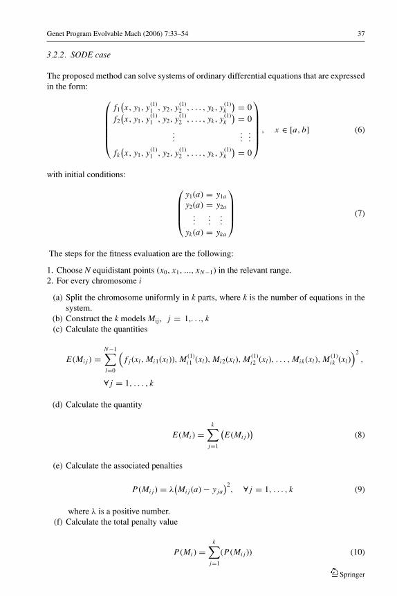
3.2.2. SODE case

The proposed method can solve systems of ordinary differential equations that are expressedin the form:

f1(x, y1, y(1)

1 , y2, y(1)2 , . . . , yk, y(1)

k

) = 0f2

(x, y1, y(1)

1 , y2, y(1)2 , . . . , yk, y(1)

k

) = 0

......

...

fk(x, y1, y(1)

1 , y2, y(1)2 , . . . , yk, y(1)

k

) = 0

, x ∈ [a, b] (6)

with initial conditions:

y1(a) = y1a

y2(a) = y2a...

......

yk(a) = yka

(7)

The steps for the fitness evaluation are the following:

1. Choose N equidistant points (x0, x1, ..., xN−1) in the relevant range.2. For every chromosome i

(a) Split the chromosome uniformly in k parts, where k is the number of equations in thesystem.

(b) Construct the k models Mij, j = 1,. . ., k(c) Calculate the quantities

E(Mi j ) =N−1∑

l=0

(f j (xl , Mi1(xl )), M (1)

i1 (xl ), Mi2(xl ), M (1)i2 (xl ), . . . , Mik(xl ), M (1)

ik (xl ))2

,

∀ j = 1, . . . , k

(d) Calculate the quantity

E(Mi ) =k∑

j=1

(E(Mi j )

)(8)

(e) Calculate the associated penalties

P(Mi j ) = λ(Mi j (a) − y ja

)2, ∀ j = 1, . . . , k (9)

where λ is a positive number.(f) Calculate the total penalty value

P(Mi ) =k∑

j=1

(P(Mi j )) (10)

Springer


(g) Finally, the fitness of the chromosome i is given by:

ui = E(Mi ) + P(Mi ) (11)

3.2.3. PDE case

We only consider here elliptic PDE’s in two and three variables with Dirichlet boundaryconditions. The generalization of the process to other types of boundary conditions andhigher dimensions is straightforward. The PDE is expressed in the form:

f

(x, y, �(x, y),

∂

∂x�(x, y),

∂

∂y�(x, y),

∂2

∂x2�(x, y),

∂2

∂y2�(x, y)

)= 0 (12)

with x ∈ [x0, x1] and y ∈ [y0, y1]. The associated Dirichlet boundary conditions are ex-pressed as: �(x0, y) = f0(y), �(x1, y) = f1(y), �(x, y0) = g0(x), �(x, y1) = g1(x).

The steps for the fitness evaluation of the population are given below:

1. Choose N2 equidistant points in the box [x0,x1] × [y0,y1], Nx equidistant points on theboundary at x = x0 and at x = x1, Ny equidistant points on the boundary at y = y0 andat y = y1.

2. For every chromosome i

� Construct a trial solution Mi(x, y) expressed in the grammar described earlier.� Calculate the quantity

E(Mi )

=N 2∑

j=1

f

(

x j , y j , Mi (x j , y j ),∂

∂xMi (x j , y j ),

∂

∂yMi (x j , y j ),

∂2

∂x2Mi (x j , y j ),

∂2

∂y2Mi (x j , y j )

)2

� Calculate the quantities

P1(Mi ) =Nx∑

j=1

(Mi (x0, y j ) − f0(y j )

)2

P2(Mi ) =Nx∑

j=1

(Mi (x1, y j ) − f1(y j )

)2

P3(Mi ) =Ny∑

j=1

(Mi (x j , y0) − g0(x j )

)2

P4(Mi ) =Ny∑

j=1

(Mi (x j , y1) − g1(x j )

)2

� Calculate the fitness of the chromosome as:

vi = E(Mi ) + λ(P1(Mi ) + P2(Mi ) + P3(Mi ) + P4(Mi )) (13)

Springer


3.2.4. A complete illustrative example

Consider the ODE

y′′ + 100y = 0, x ∈ [0, 1]

with the boundary conditions y(0) = 0 and y′(0) = 10. We take in the range [0, 1]N = 10 equidistant points x0,. . ., x9. Suppose that we have chromosomes with length 10and one chromosome is the array: g = [7, 2, 10, 4, 4, 2, 11, 20, 30, 5]. The function whichcorresponds to the chromosome g is Mg(x) = exp(x) + sin(x). The first order derivative isM (1)(x)

g = exp(x) + cos(x) and the second order derivative is M (2)(x)g = exp(x) − sin(x). The

symbolic computation of the above quantities is described in detail in the Section 2. Usingthe Eq. (3) we have:

E(Mg) =9∑

i=0

(M (2)

g (xi ) + 100Mg(xi ))2

=9∑

i=0

(101 exp(xi ) + 99 sin(xi ))2

= 4849332.4

The penalty function P(Mg) is calculated following the Eq. (5) as:

P(Mg) = λ((Mg(0) − y(0))2 + (

M (1)g (0) − )2)

= λ((exp(0) + sin(0) − 0)2 + (exp(0) − sin(0) − 10)2)

= λ((1 + 0 − 0)2 + (1 − 0 − 10)2)

= 82λ

So, the fitness value ug of the chromosome is given by:

ug = E(Mg) + P(Mg)

= 4849332.4 + 82λ

We perform the above procedure to all chromosomes in the population and we sort themin ascending order according to their fitness value. In consequence, we apply the geneticoperators, the new population is created and the process is repeated until the terminationcriteria are met.

3.3. Evaluation of derivatives

Derivatives are evaluated together with the corresponding functions using an additionalstack and the following differentiation elementary rules, adopted by the various AutomaticDifferentiation Methods [21] and used in corresponding tools [18–20]:

1. ( f (x) + g(x))′ = f ′(x) + g′(x)

Springer


2. ( f (x)g(x))′ = f ′(x)g(x) + f (x)g′(x)

3.(

f (x)g(x)

)′= f ′(x)g(x)−g′(x) f (x)

g2(x)

4. f (g(x))′ = g′(x) f ′(g(x))

To find the first derivative of a function we use two different stacks, the first is used forthe function value and the second for the derivative value. For instance consider that wewant to estimate the derivative of the function f (x) = sin(x) + log(x + 1). Suppose that S0

is the stack for the function’s value and S1 is the stack for the derivative. The function f(x)in postfix order is written as “x sin x 1 + log + ”. We begin to read from left to right,until we reach the end of the string. The following calculations are performed in the stacksS0 and S1. We denote with (a0,a1, · · ·, an) the elements in a stack, an being the element atthe top.

1. S0 = (x), S1 = (1)2. S0 = (sin(x)), S1 = (1 cos(x))3. S0 = (sin(x), x), S1 = (1 cos(x), 1)4. S0 = (sin(x), x, 1), S1 = (1 cos(x), 1, 0)5. S0 = (sin(x), x + 1), S1 = (1 cos(x), 1 + 0)6. S0 = (sin(x), log(x + 1)), S1 = (1 cos(x), 1+0

x+1 )7. S0 = (sin(x) + log(x + 1)), S1 = (1 cos(x) + 1+0

x+1 )

The S1 stack contains the first derivative of f(x). To extend the above calculations for thesecond order derivative, a third stack must be employed.

3.4. Genetic operations

3.4.1. Genetic operators

The genetic operators that are applied to the genetic population are the initialization, thecrossover and the mutation.

The initialization is applied only once on the first generation. For every element of eachchromosome a random integer in the range [0..255] is selected.

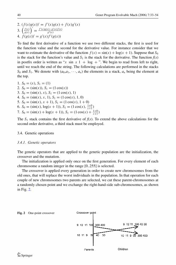
The crossover is applied every generation in order to create new chromosomes from theold ones, that will replace the worst individuals in the population. In that operation for eachcouple of new chromosomes two parents are selected, we cut these parent-chromosomes ata randomly chosen point and we exchange the right-hand-side sub-chromosomes, as shownin Fig. 2.

Fig. 2 One-point crossover

Springer


The parents are selected via tournament selection, i.e.:

� First, we create a group of K ≥ 2 randomly selected individuals from the current popula-tion.

� The individual with the best fitness in the group is selected, the others are discarded.The final genetic operator used is the mutation, where for every element in a chromosomea random number in the range [0,1] is chosen. If this number is less than or equal to themutation rate the corresponding element is changed randomly, otherwise it remains intact.

3.4.2. Application of genetic operators

In every generation the following steps are performed:

1. The chromosomes are sorted with respect to their fitness value, in a way that the bestchromosome is placed at the beginning of the population and the worst at the end.

2. c = (1 − s)∗ g new chromosomes are produced by the crossover operation, where s is thereplication rate of the model and g is the total number of individuals in the population. Thenew individuals will replace the worst ones in the population at the end of the crossover.

3. The mutation operation is applied to every chromosome excluding those which have beenselected for replication in the next generation.

3.5. Termination control

The genetic operators are applied to the population creating new generations, until a maxi-mum number of generations is reached or the best chromosome in the population has fitnessbetter than a preset threshold.

4. Experimental results

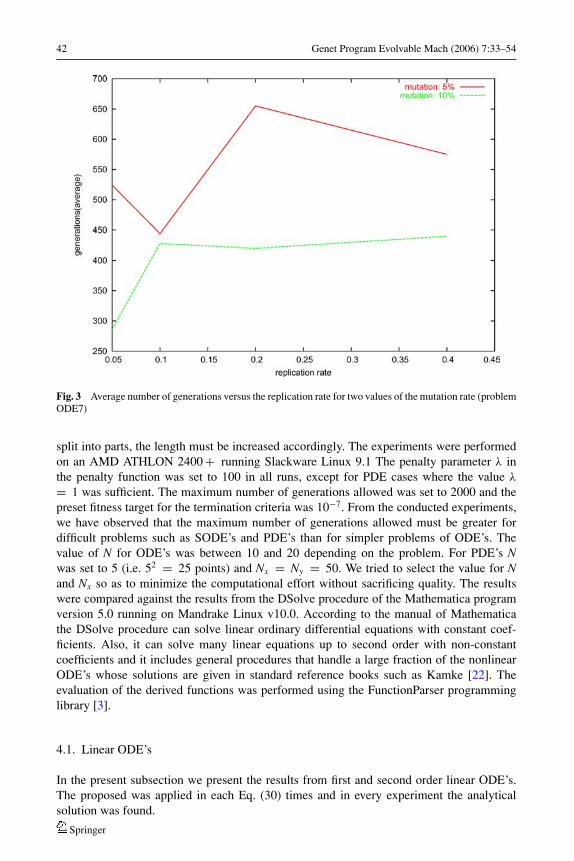
We describe several experiments performed on linear and non linear first and second orderODE’s and systems and PDE’s in two and three dimensions. In addition we applied ourmethod to ODE’s that do not posses an analytical closed form solution and hence can not berepresented exactly by the grammar. For the case of systems of ODE’s, each chromosomeis split uniformly in M parts, where M is the number of equations in the system. Each partof the chromosome represents the solution of the corresponding ODE. We used 10% for thereplication rate (hence the crossover probability is set to 90%) and 5% for the mutation rate.We investigated the importance of these two parameters by performing experiments usingsets of different values. Each experiment was performed 30 times and we plot the averagenumber of generations for the ODE7 problem in Fig. 3. As one can see the performanceis somewhat dependent on these parameters, but not critically. The population size was setto 1000 and the length of each chromosome to 50. The size of the population is a criticalparameter. Too small a size weakens the method’s effectiveness. Too big a size renders themethod slow. Hence since there is no first principals estimation for the the population size,we resorded to an experimental approach to obtain a realistic determination of its range. Itturns out that values in the interval [200, 1000] are proper. We used fixed-length chromo-somes instead of variable-length to avoid creation of unnecessary large chromosomes whichwill render the method inefficient. The length of the chromosomes is usually depended onthe problem to be solved. For the case of simple ODE’s a length between 20 and 50 isusually sufficient, while for the case of SODE’s and PDE’s where the chromosome must be

Springer


Fig. 3 Average number of generations versus the replication rate for two values of the mutation rate (problemODE7)

split into parts, the length must be increased accordingly. The experiments were performedon an AMD ATHLON 2400 + running Slackware Linux 9.1 The penalty parameter λ inthe penalty function was set to 100 in all runs, except for PDE cases where the value λ

= 1 was sufficient. The maximum number of generations allowed was set to 2000 and thepreset fitness target for the termination criteria was 10−7. From the conducted experiments,we have observed that the maximum number of generations allowed must be greater fordifficult problems such as SODE’s and PDE’s than for simpler problems of ODE’s. Thevalue of N for ODE’s was between 10 and 20 depending on the problem. For PDE’s Nwas set to 5 (i.e. 52 = 25 points) and Nx = Ny = 50. We tried to select the value for Nand Nx so as to minimize the computational effort without sacrificing quality. The resultswere compared against the results from the DSolve procedure of the Mathematica programversion 5.0 running on Mandrake Linux v10.0. According to the manual of Mathematicathe DSolve procedure can solve linear ordinary differential equations with constant coef-ficients. Also, it can solve many linear equations up to second order with non-constantcoefficients and it includes general procedures that handle a large fraction of the nonlinearODE’s whose solutions are given in standard reference books such as Kamke [22]. Theevaluation of the derived functions was performed using the FunctionParser programminglibrary [3].

4.1. Linear ODE’s

In the present subsection we present the results from first and second order linear ODE’s.The proposed was applied in each Eq. (30) times and in every experiment the analyticalsolution was found.

Springer


ODE1

y′ = 2x − y

x

with y(0) = 20.1 and x ∈ [0.1, 1.0]. The analytical solution is y(x) = x + 2x .

ODE2

y′ = 1 − y cos(x)

sin(x)

with y(0.1) = 2.1sin(0.1) and x ∈ [0.1,1]. The analytical solution is y(x) = x+2

sin(x) .

ODE3

y′ = −1

5y + exp(− x

5) cos(x)

with y(0) = 0 and x ∈ [0, 1]. The analytical solution is y(x) = exp(− x5 ) sin(x).

ODE4

y′′ = −100y

with y(0) = 0 and y′(0) = 10 and x ∈ [0, 1]. The analytical solution is y(x) = sin(10x).

ODE5

y′′ = 6y′ − 9y

with y(0) = 0 and y′(0) = 2 and x ∈ [0, 1]. The analytical solution is y(x) = 2x exp(3x).

ODE6

y′′ = −1

5y′ − y − 1

5exp

(− x

5

)cos(x)

with y(0) = 0 and y′(0) = 1 and x ∈ [0, 2]. The analytical solution is y(x) = exp(− x5 ) sin(x).

ODE7

y′′ = −100y

with y(0) = 0 and y(1) = sin (10) and x ∈ [0, 1]. The analytical solution is y(x) = sin (10x).

ODE8

xy′′ + (1 − x)y′ + y = 0

with y(0) = 1 and y(1) = 0 and x ∈ [0, 1]. The analytical solution is y(x) = 1 − x.

ODE9

y′′ = −1

5y′ − y − 1

5exp

(− x

5

)cos(x)

Springer


Table 2 Method results for linear ODE’s

ODE MIN MAX AVG

ODE1 8 1453 653ODE2 52 1816 742ODE3 23 1598 705ODE4 14 1158 714ODE5 89 1189 441ODE6 37 1806 451ODE7 42 1242 444ODE8 3 702 66ODE9 59 1050 411

with y(0) = 0 and y(1) = sin(1)exp(0.2) and x ∈ [0, 1]. The analytical solution is y(x) =

exp(− x5 ) sin(x).

In Table 2 we list the results from the proposed method for the equations above. Underthe ODE heading the equation label is listed. Under the headings MIN, MAX, AVG we listthe minimum, maximum and average number of generations (in the set of 30 experiments)needed to recover the exact solution. The Mathematica subroutine DSolve has managed tofind the analytical solution in all cases.

In Fig. 4 we plot the evolution of a trial solution for the fourth problem ofTable 2. At generation 22 the fitness value was 4200.5 and the intermediate solutionwas:

y22(x) = sin((sin(− log(4)x((− cos(cos(exp(7))) exp(cos(6))) − 5))))

At generation 27 the fitness value was 517.17 and the corresponding candidate solution was:

y27(x) = sin((sin(− log(4)x((− cos(cos(sin(7))) exp(cos(6))) − 5))))

Finally, at generation 59 the problem was solved exactly.

4.2. Non-linear ordinary differential equations

In this subsection we present results from the application of the method to non-linear ordinarydifferential equations. In all the equations the method was applied 30 times and in everyapplication the exact solution was found.

NLODE1

y′ = 1

2y

with y(1) = 1 and x ∈ [1, 4]. The exact solution is y = √x . Note that

√x does not belong

to the basis set.

NLODE2

(y′)2 + log(y) − cos2(x) − 2 cos(x) − 1 − log(x + sin(x)) = 0

with y(1) = 1 + sin (1) and x ∈ [1, 2] The exact solution is y = x + sin (x).

Springer


Fig. 4 Evolving candidate solutions of y′ = − 100y with boundary conditions on the left

NLODE3

y′′y′ = − 4

x3

with y(1) = 0 and x ∈ [1,2]. The exact solution is y = log (x2).

NLODE4

x2 y′′ + (xy′)2 + 1

log(x)= 0

with y(e) = 0, y′(e) = 1e and x ∈ [e, 2e]. The exact solution is y(x) = log (log (x)) and it was

recovered at the 30th generation. In Table 3 we list results from the application of the methodto the equations above. The meaning of the columns is the same as 2. The Mathematicasubroutine DSolve has managed to find the exact solution only for NLODE1.

In Fig. 5 we plot intermediate trial solutions of the NLODE3.At the second generation the trial solution had a fitness value of 73.512 and it assumed

the form:

y2(x) = log(x − exp(−x − 1)) − cos(5)

Table 3 Method results for non-linear ODE’s

NLODE MIN MAX AVG

NLODE1 6 945 182NLODE2 3 692 86NLODE3 4 1564 191NLODE4 6 954 161

Springer


Fig. 5 Candidate solutions of third non-linear equation

while at the fourth generation it had a fitness value of 48.96 and it became:

y4(x) = log(log(x + x))

Similarly at the 8th generation the fitness of the intermediate solution was 4.61 and itsfunctional form was:

y8(x) = sin(log(x ∗ x))

The exact solution was obtained at the 9th generation.

4.3. Systems of ODE’s

SODE1

y′1 = cos(x) + y2

1 + y2 − (x2 + sin2(x))

y′2 = 2x − x2 sin(x) + y1 y2

with y1(0) = 0, y2(0) = 0 and x ∈ [0, 1]. The exact solution is given by: y1 = sin (x), y2 =x2.

SODE2

y′1 = cos(x) − sin(x)

y2

y′2 = y1 y2 + exp(x) − sin(x)

with y1(0) = 0, y2(0) = 1 and x ∈ [0, 1]. The exact solution is y1 = sin(x)exp(x) , y2 = exp (x).

Springer


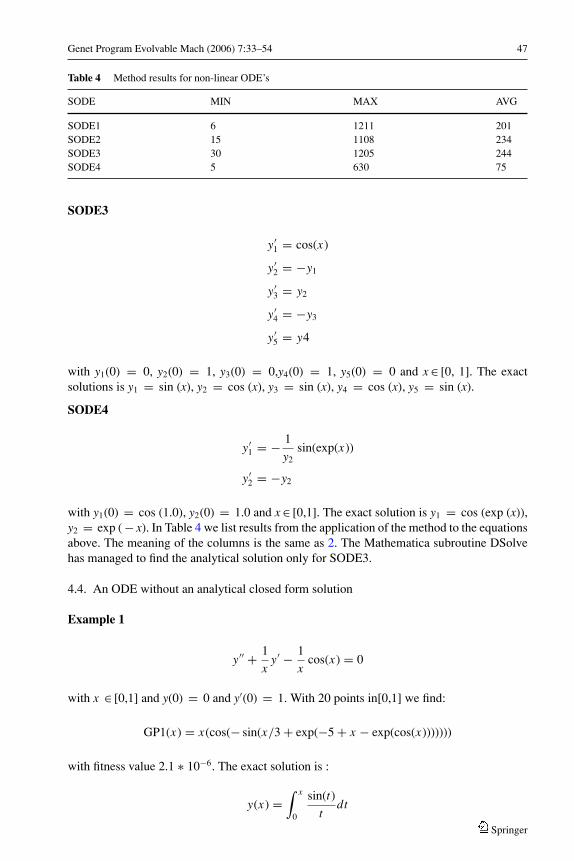
Table 4 Method results for non-linear ODE’s

SODE MIN MAX AVG

SODE1 6 1211 201SODE2 15 1108 234SODE3 30 1205 244SODE4 5 630 75

SODE3

y′1 = cos(x)

y′2 = −y1

y′3 = y2

y′4 = −y3

y′5 = y4

with y1(0) = 0, y2(0) = 1, y3(0) = 0,y4(0) = 1, y5(0) = 0 and x ∈ [0, 1]. The exactsolutions is y1 = sin (x), y2 = cos (x), y3 = sin (x), y4 = cos (x), y5 = sin (x).

SODE4

y′1 = − 1

y2sin(exp(x))

y′2 = −y2

with y1(0) = cos (1.0), y2(0) = 1.0 and x ∈ [0,1]. The exact solution is y1 = cos (exp (x)),y2 = exp ( − x). In Table 4 we list results from the application of the method to the equationsabove. The meaning of the columns is the same as 2. The Mathematica subroutine DSolvehas managed to find the analytical solution only for SODE3.

4.4. An ODE without an analytical closed form solution

Example 1

y′′ + 1

xy′ − 1

xcos(x) = 0

with x ∈ [0,1] and y(0) = 0 and y′(0) = 1. With 20 points in[0,1] we find:

GP1(x) = x(cos(− sin(x/3 + exp(−5 + x − exp(cos(x)))))))

with fitness value 2.1 ∗ 10−6. The exact solution is :

y(x) =∫ x

0

sin(t)

tdt

Springer


Fig. 6 Plot of GP1(x) and y(x) = ∫ x0

sin(t)t dt

In Fig. 6, we plot the two functions in the range [0,5]

Example 2

y′′ + 2xy = 0

with x ∈ [0,1] and y(0) = 0 and y′(0) = 1. The exact solution is :

y(x) =∫ x

0exp(−t2)dt

With 20 points in [0,1] we find:

GP2(x) = sin(sin(x + exp(exp(x) log(9)/ exp(8 + cos(1))/(exp(7/ exp(x)) + 6)))

with fitness 1.7 ∗ 10−5. In Fig. 7 we the plot the two functions in the range [0, 5].Observe, that even though the equations in the above examples were solved for x ∈ [0,

1], the approximation maintains its quality beyond that interval, a fact that illustrates theunusual generalization ability.

4.5. A special case

Consider the ODE

y′′(x2 + 1) − 2xy − x2 − 1 = 0

in the range [0, 1] and with initial conditions y(0) = 0 and y′(0) = 1. The analytical solutionis y(x) = (x2 + 1)arctan(x). Note that arctan(x) does not belong to the function repertoire ofthe method and this make the case special. The solution reached is not exact but approximate

Springer


Fig. 7 Plot of GP2(x) and y(x) = ∫ x0 exp(−t2)dt

given by:

GP(x) = x/ sin(exp(cos(5/4/ exp(x)) − exp((− exp(((−((− exp(cos(sin(2x))))))))))))

with fitness 0.0059168. Note that the subroutine DSolve of Mathematica failed to solve theabove equation. In Fig. 8 we plot z(x) ( obtained using the method of Lagaris et al. [5]), y(x)= (x2 + 1)arctan(x) (which is the exact solution) and the above solution GP(x). From Figs.6–8 we observe the quality of the approximate solution even outside the training interval,hence rendering our method useful and practical.

4.6. PDE’s

In this subsection we present results from the application of the method to elliptic partialdifferential equations. In all the equations the method was applied 30 times and in everyapplication the exact solution was found.

PDE1

∇2�(x, y) = exp(−x)(x − 2 + y3 + 6y)

with x ∈ [0, 1] and y ∈ [0, 1] and boundary conditions: �(0, y) = y3, �(1, y) =(1 + y3) exp(−1), �(x, 0) = x exp(−x), �(x, 1) = (x + 1) exp(−x). The exact solution is�(x, y) = (x + y3) exp(−x).

PDE2

∇2�(x, y) = −2�(x, y)

Springer


Fig. 8 z(x), y(x) = (x2 + 1)arctan(x), GP(x)

with x ∈ [0, 1] and y ∈ [0, 1] and boundary conditions: �(0, y) = 0, �(1, y) = sin(1) cos(y),�(x, 0) = sin(x), �(x, 1) = sin(x) cos(1). The exact solution is �(x, y) = sin(x) cos(y).

PDE3

∇2�(x, y) = 4

with x ∈ [0, 1] and y ∈ [0, 1] and boundary conditions: �(0, y) = y2 + y + 1, �(1, y) =y2 + y + 3, �(x, 0) = x2 + x + 1, �(x, 1) = x2 + x + 3. The exact solution is �(x, y) =x2 + y2 + x + y + 1.

PDE4

∇2�(x, y) = −(x2 + y2)�(x, y)

with x ∈ [0, 1] and y ∈ [0, 1] and boundary conditions: �(x, 0) = 0, �(x, 1) = sin(x),�(0, y) = 0, �(1, y) = sin(y). The exact solution is �(x, y) = sin(xy).

PDE5

∇2�(x, y) = (x − 2) exp(−x) + x exp(−y)

with x ∈ [0, 1] and y ∈ [0, 1] and boundary conditions: �(x, 0) = x(exp(−x) + 1), �(x, 1) =x(exp(−x) + exp(−1)), �(0, y) = 0, �(1, y) = exp(−y) + exp(−1). The exact solution is�(x, y) = x(exp(−x) + exp(−y)).

PDE6

Springer


Table 5 Method results for PDE’s

PDE MIN MAX AVG

PDE1 159 1772 966PDE2 5 1395 203PDE3 18 311 154PDE4 4 1698 207PDE5 195 945 444PDE6 185 1579 797PDE7 10 1122 325

The following is a highly non-linear pde:

∇2�(x, y) + exp(�(x, y)) = 1 + x2 + y2 + 4

(1 + x2 + y2)2

with x ∈ [ − 1, 1] and y ∈ [ − 1, 1] and boundary conditions: f (0, y) = log(1 + y2),f (1, y) = log(2 + y2), g(x, 0) = log(1 + x2) and g(x, 1) = log(2 + x2). The exact solutionis �(x, y) = log(1 + x2 + y2).

PDE7

∇2�(x, y, z) = 6

with x ∈ [0, 1] and y ∈ [0, 1] and z ∈ [0, 1] and boundary conditions: �(0, y, z) = y2 +z2, �(1, y, z) = y2 + z2 + 1, �(x, 0, z) = x2 + z2, �(x, 1, z) = x2 + z2 + 1, �(x, y, 0) =x2 + y2, �(x, y, 1) = x2 + y2 + 1. The exact solution is �(x, y, z) = x2 + y2 + z2 + 1.

In Table 5 we list results from the application of the method to the equations above.The meaning of the columns is the same as 2. The Mathematica subroutine DSolve has notmanaged to find the exact solution for any of the examples above.

In the following we present some graphs for trial solutions of the second PDE. Atgeneration 1 the trial solution was

GP1(x, y) = x

7

with fitness value 8.14. The difference between the trial solution GP1(x,y) and the exactsolution �(x,y) is shown in Fig. 9. At the 10thgeneration the trial solution was

GP10(x, y) = sin(x/3 + x)

with fitness value 3.56. The difference between the trial solution GP10(x,y) and the exactsolution �(x,y) is shown in Fig.10.At the 40th generation the trial solution was

GP40(x) = sin(cos(y)x)

with fitness value 0.59. The difference between the trial solution GP40(x, y) and the exactsolution �(x,y) is shown in Fig. 11.

Springer


Fig. 9 Difference between�(x, y) = sin(x) cos(y) andGP1(x,y)



5. Conclusions and further work

We presented a novel approach for solving ODE’s and PDE’s. The method is based on geneticprogramming. This approach creates trial solutions and seeks to minimize an associated error.The advantage is that our method can produce trial solutions of highly versatile functionalform. Hence the trial solutions are not restricted to a rather inflexible form that is imposedfrequently by basis-set methods that rely on completeness. If the grammar has a rich function

Springer


repertoire, and the differential equation has a closed form solution, it is very likely that ourmethod will recover it. If however the exact solution can not be represented in a closed form,our method will produce a closed form approximant.

The grammar used in this article can be further developed and enhanced. For instance it isstraight forward to enrich the function repertoire or even to allow for additional operations.Treating different types of PDE’s with the appropriate boundary conditions is a topic ofcurrent interest and is being investigated. Our preliminary results are very encouraging.

References

1 J. D. Lambert, Numerical methods for Ordinary Differential Systems: The Initial Value Problem, JohnWiley & Sons: Chichester, England, 1991.

2 J. R. Koza, Genetic Programming: On the Programming of Computer by Means of Natural Selection.MIT Press: Cambridge, MA, 1992.

3 J. Nieminen and J. Yliluoma, “Function Parser for C++, v2.7”, available fromhttp://www.students.tut.fi/̃ warp/FunctionParser/.

4 G. E. Fasshauer, “Solving differential equations with radial basis functions: Multilevel methods andsmoothing,” Advances in Computational Mathematics, vol. 11, nos. 2–3, pp. 139–159, 1999.

5 I. Lagaris, A. Likas, and D. I. Fotiadis, “Artificial neural networks for solving ordinary and par-tial differential equations,” IEEE Transactions on Neural Networks, vol. 9, no. 5, pp. 987–1000,1998.

6 G. Burgess, “Finding approximate analytic solutions to differential equations using genetic program-ming,” Surveillance Systems Division, Electronics and Surveillance Research Laboratory, Department ofDefense, Australia, 1999.

7 H. Cao, L. Kang, Y. Chen, and J. Yu, Evolutionary modeling of systems of ordinary differential equationswith genetic programming, Genetic Programming and Evolvable Machines, vol. 1, pp. 309–337,2000.

8 H. Iba and E. Sakamoto,: “Inference of differential equation models by genetic programming,” Proceedingsof the Genetic and Evolutionary Computation Conference (GECCO 2002), 2002, pp. 788–795.

9 M. O’ Neill, Automatic Programming in an Arbitrary Language: Evolving Programs with GrammaticalEvolution. PhD thesis, University Of Limerick, Ireland, August 2001.

10 C. Ryan, J. J. Collins, and M. O’ Neill, Evolving programs for an arbitrary language, in Proceedings ofthe First European Workshop on Genetic Programming, volume 1391 of LNCS, W. Banzhaf, Ri. Poli, M.Schoenauer, and T. C. Fogarty, (eds.), Springer-Verlag, pp. 83–95, Paris, 14–15 April 1998.

11 M. O’Neill and C. Ryan, Grammatical Evolution: Evolutionary Automatic Programming in a ArbitraryLanguage, volume 4 of Genetic programming. Kluwer Academic Publishers, 2003.

12 C. Ryan, M. O’Neill, and J. J. Collins, “Grammatical evolution: Solving trigonometric identities,” inProceedings of Mendel 1998: 4th International Mendel Conference on Genetic Algorithms, OptimizationProblems, Fuzzy Logic, Neural Networks, Rough Sets., Brno, Czech Republic, June 24–26 1998.Technical University of Brno, Faculty of Mechanical Engineering, pp. 111–119.

13 M. O’Neill and C. Ryan, “Grammatical evolution,” IEEE Trans. Evolutionary Computation, vol. 5, pp.349–358, 2001.

14 D. E. Goldberg, Genetic algorithms in search, Optimization and Machine Learning, Addison Wesley, 1989.15 J. J. Collins and C. Ryan, “Automatic generation of robot behaviors using grammatical evolution,” in

Proc. of AROB 2000, the Fifth International Symposium on Artificial Life and Robotics.16 M. O’Neill, J. J. Collins, and C. Ryan, “Automatic generation of caching algorithms,” in Evolutionary

Algorithms in Engineering and Computer Science, Kaisa Miettinen, Marko M. Mkel, Pekka Neittaanmki,and Jacques Periaux (eds.), Jyvskyl, Finland, 30 May–3 June 1999, John Wiley & Sons, pp. 127–134,1999.

17 A. Brabazon and M. O’Neill, “A grammar model for foreign-exchange trading,” in Proceedings of theInternational conference on Artificial Intelligence, volume II, H. R. Arabnia et al. (eds.), CSREA Press,23–26 June 2003, pp. 492–498, 2003.

18 P. Cusdin and J. D. Muller, “Automatic differentiation and sensitivity analysis methods for CFD,” QUBSchool of Aeronautical Engineering, 2003.

19 O. Stauning, “Flexible automatic differentiation using templates and operator overloading in C++,” Talkpresented at the Automatic Differentiation Workshop at Shrivenham Campus, Cranfield University, June6, 2003.

Springer


20 C. Bischof, A. Carle, G. Corliss, and A. Griewank, “ADIFOR - generating derivative codes from fortranprograms,” Scientific Programming, no. 1, pp. 1–29, 1992.

21 A. Griewank, “On automatic differentiation” in Mathematical programming: Recent Developmentsand Applications, M. Iri and K. Tanabe (eds.), Kluwer Academic Publishers, Amsterdam, pp. 83–108,1989.

22 E. Kamke, Differential Equations. Solution Methods and Solutions, Teubner, Stuttgart, 1983.

Springer

solving differential equations with genetic programminglagaris/papers/degen.pdf · genet program...

Documents