solving design equations for a hollow fiber bioreactor with arbitrary kinetics

Chemical Engineering Journal 84 (2001) 445–461

Solving design equations for a hollow fiberbioreactor with arbitrary kinetics

Marıa I. Cabrera1, Julio A. Luna2, Ricardo J. Grau∗,2Instituto de Desarrollo Tecnológico para la Industria Quımica (INTEC), Universidad Nacional del Litoral and CONICET,

Güemes 3450, 3000 Santa Fe, Argentina

Received 12 May 1999; received in revised form 3 October 2000; accepted 4 October 2000

Abstract

An approach for solving the hollow fiber bioreactor design equations is presented. The original set of differential mass balance equationsis cast into an equivalent system of integral equations by generating the appropriate Green’s functions. Mathematical features commonto all hollow fiber bioreactors (HFBRs) operating with laminar flow are imbedded in the corresponding Green’s functions on the lumenside, and thus separated from specific aspects arising from mass transport through the permeable wall. On the spongy matrix side, theappropriate Green’s functions are expressed in terms of the mass transfer properties without involving any chemical kinetic parameters;this avoids repetitive computational effort when treating different reaction kinetics.

The derived integral equations are numerically solved on an appropriately transformed coordinate system. The numerical method is wellsuited for problems where steep gradients of concentration cause an inaccurate numerical integration and low rates of convergence if theequations are solved with a uniform rectangular grid on the original coordinate system. The effectiveness of the proposed approach forthe simulation of HFBRs with power-law, Michaelis–Menten and zero-order kinetics is demonstrated. The method is readily extendible totreat problems with chemical kinetics described by any arbitrary functional form. © 2001 Elsevier Science B.V. All rights reserved.

Keywords:Hollow fiber bioreactor; Design integral equations; Arbitrary kinetics; Green’s functions; Iterative computation method

1. Introduction

Advances in the integration of permeable and selectivemembranes with biological catalysts such as live cells andenzymes provide the basis to develop competitive biopro-cessing schemes. Several configurations having a bundleof hollow fibers as core of the membrane device are usedin diverse applications including reverse osmosis, ultrafil-tration, dialysis, and biocatalyst immobilization. After thesuccessful use of hollow fiber bioreactors (HFBRs) for thecultivation of mammalian cells [1], HFBRs have found ap-plications in enzymatic reactions, microbial fermentations,animal cell culture and plant cell culture [2–4].

Consequently, the design and simulation of HFBRs hasbeen dealt with in different ways and with different levels ofsimplification [5]. In this regard, several papers have beenwritten among which we can cite some of the best knownfundamental contributions from the numerical solution

∗ Corresponding author. Fax:+54-342-4550944.E-mail address:[email protected] (R.J. Grau).

1 Member of CONICET’s Research Staff.2 Professor at UNL and Member of CONICET’s Research Staff.

viewpoint. Exact analytic expressions for the substrate con-centration profile throughout an HFBR have been deducedfor a first-order reaction rate using an integral formulationand solving Michaelis–Menten kinetics by numerical finitedifference [6]. Analytic solutions have been developed interms of Kummer functions with constants depending onthe value of the Sherwood number at the permeable wall[7]. Models utilising effectiveness factors for both first- andzero-order kinetics have been developed [8]. A mathemat-ical analysis of oxygen depletion has been performed inorder to develop effectiveness factor plots to aid in thescaling of HFBRs [9]. A non-linear mixed-type problemsimilar to that described for HFBRs has been solved bya non-iterative finite difference method [10,11] or by aniterative fourth-order Runge–Kutta–Gill algorithm [12]. Aprocedure based on a Crank–Nicolson discretization hasbeen developed to solve a generalized mathematical modelfor describing annular reactors and HFBRs as particularapplications [13]. Methodologies for simplifying the solu-tion of HFBR design equations have been described for thefirst-order and zero-order limits of the Michaelis–Mentenkinetics [14,15]. Numerical solutions are required tosolve zero-order kinetics with substrate exhaustion, but

1385-8947/01/$ – see front matter © 2001 Elsevier Science B.V. All rights reserved.PII: S1385-8947(00)00269-2

446 M.I. Cabrera et al. / Chemical Engineering Journal 84 (2001) 445–461

Nomenclature

a inner radius of the membrane (cm)An normalization constant for thenth

eigenfunction (dimensionless)b outer radius of the membrane (cm)c concentration (mol cm−3)c array of concentrations in the spongy matrix

region (mol cm−3)C c/c0, concentration (dimensionless)C array of concentrations in the spongy matrix

region (dimensionless)Cb averaged bulk concentrations (dimensionless)d outer radius of the spongy matrix wall (cm)D diffusion coefficient of substrate (cm2 s−1)G Green’s functionGe a/L, geometrical parameter (dimensionless)H −DIIKa/DI ln(a/b), membrane mass transfer

coefficient (dimensionless)J JacobianK Kb/Ka , lumen/spongy matrix partition

coefficient (dimensionless)Ka lumen/membrane partition coefficient

(dimensionless)Kb membrane/spongy matrix partition coefficient

(dimensionless)KM Michaelis–Menten constant (mol cm−3)L hollow fiber length (cm)Le entrance length (cm)M confluent hypergeometric functionn reaction orderN total number of species in the systemPe Vmx a/D

I , Peclet number (dimensionless)r radial coordinate (cm)R reaction rate (s−1)Re 2aVmxρ/µ, Reynolds number (dimensionless)VM maximum reaction rate (s−1)Vmx maximum velocity (cm s−1)z axial coordinate (cm)

Greek lettersαζ , αϕ parameters in Eqs. (70) and (71)β d/b, parameter (dimensionless)δ Dirac delta functionζ dimensionless transformed axial coordinateϕ dimensionless transformed radial coordinateΘ step functionλn nth eigenvalue defined by Eq. (24)µ viscosity (P)ν stoichiometric coefficientξ z/L (dimensionless axial coordinate)ρ r/a (zone I) orr/b (zone III)

(dimensionless radial coordinate);density (g cm−3)

φn nth eigenfunction defined by Eq. (23)Φ Thiele modulus,(b2VM(c

0)n−1/DIII )1/2

for power-law kinetics,(b2VM/KM DIII )1/2

for Michaelis–Menten kinetics, and(b2VM/c

0DIII )1/2 for zero-order kineticsΩ b2RIII /c0DIII (dimensionless reaction rate)

SuperscriptsI, II, III lumen, fiber, and spongy matrix regions,

respectively0 at the reactor inlet

Subscriptsc at critical boundaryi denotes componentin nth value

analytical solutions in terms of Kummer functions arepossible for either first-order or zero-order with substrateremaining constant everywhere in the HFBR. An extensionto treat first-order kinetics and power-law-type fluids hasbeen presented [16]. A method based on the shooting tech-nique has been proposed to avoid problems accompanyingthe application of the orthogonal collocation on finite el-ements [17]. Finite difference and orthogonal collocationmethods have been used to solve dynamic models of HF-BRs [18–21]. Also, the mathematical modelling of HFBRshas been reviewed with illustrative computational modelcalculations [5].

This work deals with the solution of the HFBR designequations for the case in which the kinetics may be de-scribed by any arbitrary function. The original set of differ-ential balance equations with the corresponding initial andboundary conditions is turned into an equivalent systemof integral equations that represents the formal solution tothe original differential problem. On the lumen side, thespecies mass balance equation is expressed in terms ofeigenfunctions whose eigenvalues do not depend on thevalue of the Sherwood number at the permeable wall. Thisis particularly advantageous since in contrast with other re-sults once the eigenvalues are calculated, they become a setof values which is valid for all cases. On the spongy matrixside, the governing differential equation for the substrate iscast in terms of an integral equation by the definition of aGreen’s function which depends neither on the functionalform of the kinetic equation nor on the value of the kineticparameters. Thus, this generalized formulation is valid forany arbitrary kinetic equation, including zero-order reactionrate with substrate depleted before reaching the outer annu-lar wall. For the last case, an unmatched expression uponthe knowledge of the critical radius at any axial position isobtained in terms of characteristic parameters of the HFBR.

Efficient numerical schemes of solution are designed bymeans of a simple iterative process along the permeable walland through the spongy matrix, without having to resort to

M.I. Cabrera et al. / Chemical Engineering Journal 84 (2001) 445–461 447

the complete concentration profiles in the lumen. Since sig-nificant concentration gradients may truly exist in HFBRs[22], it is showed that the integral equations can be solvedvery efficiently using a continuous coordinate transformationfrom a variable grid, which has a severe stretching in regionswith steep changes of concentration, to another fixed one.Consequently, an improved accuracy of the solution with-out wasting computer memory space and running time isobtained. The computations are quite simple and faster thanthe one corresponding to the original integral equations. Theflexibility of the proposed iterative scheme is demonstratedthrough its application to several types of kinetic equations.Comparative convergence maps are presented in terms ofthe model parameters.

For zero-order kinetics, maps to know a priori if the sub-strate concentration drops to zero inside the spongy matrixare given in terms of the parameters of the HFBR model.The one-dimensional free-boundary problem which arises ifthe substrate becomes depleted at the so-called critical ra-dius is efficiently solved using any standard method to solvezeros of non-linear equations.

2. Assumptions and mathematical model

A schematic representation of a conventional HFBR isshown in Fig. 1, where a cross-sectional view of an individ-ual hollow fiber in the HFBR shows three regions. Region Iis the lumen (inner tube), region II is the permeable mem-brane (wall of the inner tube), and region III is the spongymatrix (annular region) inside which an active biocatalystin the form of either enzymes or live cells is immobilized.The substrate solution is fed through the lumen and diffusesinside out through the permeable membrane to react by cat-alytic effect of active enzymes or live cells supported on thespongy matrix. The product diffuses back to the lumen andflows downstream.

The physical model for steady-state and isothermal regimeincludes the following simplifying assumptions: For region

Fig. 1. Schematic diagram of the hollow fiber bioreactor with laminar velocity profile in the lumen region: (a) axial cross-section, and (b) radialcross-section.

I: (i) laminar flow with parabolic and totally developed ve-locity profile, (ii) negligible axial diffusion with respect tothe convective flux, (iii) Fickian diffusion in the radial direc-tion, (iv) absence of homogeneous reaction rate in the bulkof the lumen, (v) constant physical properties. For regionII: (vi) inert membrane, (vii) axial diffusion and convec-tive flux negligible with respect to the radial diffusion, (viii)mass transfer and partition coefficients are constants. Forregion III: (ix) axial diffusion and convective transport areneglected in all regions, and (x) kinetics model is describedby any arbitrary function of the reactant concentrations.

The governing mass balance differential equations for theith species in each of the three regions are:

DIi

1

r

∂

∂r

[r∂

∂rcIi (r, z)

]− 2Vmx

[1 − r2

a2

]∂

∂zcIi (r, z)

= 0, 0 < r < a, 0 < z < L (1)

DIIi

1

r

∂

∂r

[r∂

∂rcIIi (r, z)

]= 0, a < r < b, 0 < z < L (2)

DIIIi

1

r

∂

∂r

[r∂

∂rcIIIi (r, z)

]− νiR

III (c(r, z))

= 0, b < r < d, 0 < z < L (3)

with the boundary conditions:

DIi

∂

∂rcIi (0, z) = 0 (4)

DIi

∂

∂rcIi (a, z) = DII

i

∂

∂rcIIi (a, z) with Ka

i = cIIi (a, z)

cIi (a, z)

(5)

DIIi

∂

∂rcIIi (b, z) = DIII

i

∂

∂rcIIIi (b, z) with Kb

i = cIIIi (b, z)

cIIi (b, z)

(6)

DIIIi

∂

∂rcIIIi (d, z) = 0 if cIII

i (d, z) ≥ 0 (7a)


DIIIi

∂

∂rcIIIi (rc, z) = 0 if cIII

i (rc, z) = 0 for b ≤ rc < d

(7b)

and with the initial conditions:

cIi (r,0) = cI0

i (r) for i = reactant (8a)

cIi (r,0) = 0 for i = reactant (8b)

By using the following definitions,

Ci = ci

c0i

(9)

ρ =

r

a, zone I

r

b, zone III

(10)

ξ = z

L(11)

Ge= a

L(12)

Pei = Vmx a

DIi

(13)

Hi = −DIIi

DIi

Kai

ln(a/b)(14)

and taking advantage of the special definition of the dimen-sionless radial coordinate, the mass balance equation in themembrane can be written after analytical integration as amodified boundary condition atρ = 1. This boundary con-dition lumps the mass balance in the membrane and couplesdirectly the dimensionless mass balance equations in the lu-men and spongy matrix regions [10,14]. This is very usefulfor further numerical integration purposes because the num-ber of differential equations to be solved reduces from threeto two in the domain 0≤ ρ ≤ β and 0≤ ξ ≤ 1, as follows:

1

ρ

∂

∂ρ

[ρ∂

∂ρCIi (ρ, ξ)

]− 2Ge Pei [1 − ρ2]

∂

∂ξCIi (ρ, ξ)

= 0, 0 < ρ < 1, 0 < ξ < 1 (15)

1

ρ

∂

∂ρ

[ρ∂

∂ρCIIIi (ρ, ξ)

]− νiΩ

III (C(ρ, ξ))

= 0, 1 < ρ < β, 0 < ξ < 1 (16)

with boundary conditions given by

∂

∂ρCIi (ρ, ξ)

∣∣∣∣ρ=0

= 0 (17)

∂

∂ρCIi (ρ, ξ)

∣∣∣∣ρ=1

− Hi [CIi (1, ξ) − KiC

IIIi (1, ξ)] = 0 (18)

∂

∂ρCIIIi (ρ, ξ)

∣∣∣∣ρ=β

= 0 if CIIIi (β, ξ) ≥ 0 (19a)

∂

∂ρCIIIi (ρ, ξ)

∣∣∣∣ρ=ρc

= 0

if CIIIi (ρc, ξ) = 0 for 1 ≤ ρc < β (19b)

and with the following initial condition:

CIi (ρ,0) = CI0

i (ρ) for i = reactant (20a)

CIi (ρ,0) = 0 for i = reactant (20b)

Eq. (18) lumps the mass balance in the membrane.Eqs. (19a) and (19b) account for either the fixed bound-ary value problem or the free boundary value problemarising for certain kinetic models. As a complete deple-tion of substrate cannot occur for all non zero-order re-action rates, then Eq. (19a) is always fulfilled for nonzero-order kinetic models [13,15]. However, two situa-tions can be identified for the zero-order reaction rate:(a) the substrate concentration does not become zero atany point within the spongy matrix, thus Eq. (19a) isultimately fulfilled; and (b) the substrate concentrationdrops to zero at some pointρc within the spongy ma-trix, thus Eq. (19b) must be satisfied instead of Eq. (19a).The boundary value problem with Eq. (19b) is known asa free boundary problem because the location at whichthe substrate becomes depleted,ρc, is not previouslyknown.

All these boundary conditions are taken into consid-eration because there is no restriction on the functionalform of the dimensionless kinetic equation to be spec-ified for each particular application. The most generalcase of non-linear kinetics model will be mathematicallytreated by settingΩ III (C(ρ, ξ)) as any arbitrary functionof the species concentrations,C(CIII

1 , . . . , CIIIi , . . . , CIII

N ).As a particular case, the solution for zero-order kineticswill be derived from the general solution to be obtainedfurther on.

For simplicity, from now on the subindexi will be droppedfrom the dimensionless parameters and concentration of theith species.

3. Design equations in terms of integral equations

3.1. Lumen region

To transform differential mass balance equations, like toEq. (15), into their equivalent integral equations we have suc-cessfully applied an approach which consists of four steps:(1) define an appropriate differential problem for Green’sfunction which leads to a suitable form of the formal inte-gral solution, (2) identify Green’s function by comparing theexpression of the formal solution with that corresponding toits generalized Fourier expansion, (3) solve the associatedhomogeneous eigenvalue problem, and finally, (4) overcomethe difficulty introduced by the fact that any function with


simple jump discontinuities cannot be uniformly approxi-mated by a Fourier series in an interval close to the discon-tinuity (problem known as Gibbs phenomenon), as it is thecase with the non-homogeneous boundary condition givenby Eq. (18). This approach was used to solve the designequations for mass transfer in dialyzers [23], in packed-bedwith adsorption at the wall and bulk reaction [24], in tubu-lar reactors with heterogeneous reactions [25–28], and forreactive systems involving Couette flows [29,30].

Because Eqs. (15), (17) and (18) are quite similar tothose treated in previous contributions, we need not presentdetails of the transformation to the corresponding integralequation and shall write only the resulting final expression[23,25,26,28,31]:

CI(ρ, ξ) =[ ∞∑

1

φn(1)φn(ρ)

A2nλ

2n

− (ρ2 − 1

4ρ4 − 7

24)

]

×H [CI(1, ξ) − KCIII (1, ξ)]

+∫ 1

0dρ ρ(1 − ρ2)GI(ρ, ξ/ρ,0)CI(ρ,0)

− 1

2Ge Pe

∫ ξ

0dξ GI(ρ, ξ/1, ξ )H [CI(1, ξ )

−KCIII (1, ξ )] (21)

On the right-hand side of Eq. (21), the first term accountsfor the non-zero gradients at the permeable wall imposedby the non-homogeneous boundary condition atρ = 1; thesecond term can be identified as the contribution of the inletcondition, and the last one takes into account the speciesmass transfer through the permeable wall [23,25,26].

Green’s function is the following Fourier expansion[31]:

GI(ρ, ξ/ρ, ξ ) =∞∑0

A−2n exp

[− λ2

n

2Ge Pe(ξ − ξ )

]

×φn(ρ)φn(ρ)Θ(ξ − ξ ) (22)

where φn(ρ) and λn are orthogonal eigenfunctions andeigenvalues, respectively, given by

φn(ρ) = exp

[−λnρ

2

2

]M

(2 − λn

4,1, λnρ

2)

(23)

λn

[1 − λn

2

]M

(6 − λn

4,2, λn

)− M

(2 − λn

4,1, λn

)= 0 (24)

with A2n normalization coefficients defined by∫ 1

0dρ ρ(1 − ρ2)φn(ρ)φm(ρ) = A2

nδnm (25)

whereM is Kummer’s function [32] andδnm is the Kro-necker delta.

To calculate the numerical values ofCI(ρ, ξ) usingEq. (21), it is necessary to know beforehand the axialconcentration profile at the permeable wall. Accordingto Eq. (21) for ρ = 1, such concentration profile maybe obtained by a simple iterative scheme at the wallusing:

CI(1, ξ) =[ ∞∑

1

φn(1)φn(1)

A2nλ

2n

− 11

24

]H [CI(1, ξ)

−KCIII (1, ξ)]

+∫ 1

0dρ ρ(1 − ρ2)GI(1, ξ/ρ,0)CI(ρ,0)

− 1

2Ge Pe

∫ ξ

0dξ GI(1, ξ/1, ξ )H [CI(1, ξ )

−KCIII (1, ξ )] (26)

where the values ofCIII (1, ξ) may also be evaluated quicklyby using a simple iterative scheme based on the integralequation to be immediately deduced for the substrate in thespongy matrix.

3.2. Spongy matrix region

If the substrate concentration does not become de-pleted at some intermediate position in the reactor an-nulus, the handling of spatial discontinuities imposed bythe boundary conditions is straightforward because theirlocation is fixed (Case (a)). The problem becomes moredifficult to handle if the substrate concentration drops tozero at some pointρc within the spongy matrix region.In such case, only the zone 1< ρ < ρc is effective forreaction and, therefore, Eq. (16) must be solved in thespace domain with substrate concentration greater thanzero (Case (b)). Both cases are treated systematically asfollows.

As a starting point, the governing local equation for thesubstrate concentration is advantageously expressed as a lo-cal field equation which is entirely valid in the whole an-nular space even if the substrate concentration is not finiteeverywhere inside the reactor annulus. For such purpose, anindicator function is defined as

Θ(ρc − ρ) =

1 if ρc ≥ ρ

0 if ρc < ρ(27)

Θ(ρc −ρ) being a Heaviside step function whose derivativeis given by

d

dρΘ(ρc − ρ) = −δ(ρc − ρ) (28)

whereδ(ρc − ρ) is the generalized delta function [33].Using the indicator function as follows:

Θ(ρc − ρ)

1

ρ

∂

∂ρ

[ρ∂

∂ρCIII (ρ, ξ)

]− νΩ III (C(ρ, ξ))

= 0, 1 < ρ < β, 0 < ξ < 1 (29)


the governing differential equation for substrate concentra-tion can be now expressed as

1

ρ

∂

∂ρ

ρ∂

∂ρ[Θ(ρc − ρ)CIII (ρ, ξ)]

−Θ(ρc − ρ)νΩ III (C(ρ, ξ))

= −δ(ρc − ρ)∂

∂ρCIII (ρ, ξ)

− 1

ρ

∂

∂ρ[ρδ(ρc − ρ)CIII (ρ, ξ)],

1 < ρ < β, 0 < ξ < 1 (30)

which, unlike Eq. (16), is a field equation because it is validin all the space domain occupied by the spongy matrix.

Thus, in turn, the boundary conditions given by Eqs. (18)and (19a) become

∂

∂ρ[Θ(ρc − ρ)CI(ρ, ξ)]

∣∣∣∣ρ=1

+ H [Θ(ρc − 1)CI(1, ξ)

−KΘ(ρc − 1)CIII (1, ξ)] = δ(ρc − 1)CIII (1, ξ) (31)

∂

∂ρ[Θ(ρc − ρ)CIII (ρ, ξ)] − δ(ρc − ρ)CIII (ρ, ξ)

∣∣∣∣ρ=β orρc

= 0 (32)

One may notice that if there is total depletion of the sub-strate, local sources arise from the discontinuity atρ = ρc.Otherwise, Eqs. (30)–(32) become Eqs. (16), (18), (19a) and(19b). In accordance with the properties of a Dirac function,these field equations have full significance under an integraloperator.

To obtain the integral formal solution, an integra-tion of Eq. (30) is performed withρ as weight functionand with a test functionGIII (ρ/ρ), still unspecified, asfollows:

∫ β

1dρ GIII (ρ/ρ)

∂

∂ρ

ρ∂

∂ρ[Θ(ρc − ρ)CIII (ρ, ξ)]

= +ν

∫ β

1dρ ρGIII (ρ/ρ)Θ(ρc − ρ)Ω III (C(ρ, ξ))

−∫ β

1dρ ρGIII (ρ/ρ)δ(ρc − ρ)

∂

∂ρCIII (ρ, ξ)

−∫ β

1dρ GIII (ρ/ρ)

∂

∂ρ[ρδ(ρc − ρ)CIII (ρ, ξ)] (33)

Successive integrations by parts on the left-hand sideof Eq. (33), followed by some rearrangements takinginto account Eqs. (31) and (32), lead to the followingequation:

∫ β

1dρ Θ(ρc − ρ)CIII (ρ, ξ)

∂

∂ρ

ρ∂

∂ρGIII (ρ/ρ)

= +ν

∫ β


+Θ(ρc − 1)CIII (1)∂

∂ρGIII (ρ/ρ)

∣∣∣∣ρ=1

−Θ(ρc − 1)GIII (ρ/1)∂

∂ρCIII (ρ, ξ)

∣∣∣∣ρ=1

−βΘ(ρc − β)CIII (β)∂

∂ρGIII (ρ/ρ)

∣∣∣∣ρ=β

+Θ(ρc − β)GIII (ρ/β)∂

∂ρCIII (ρ, ξ)

∣∣∣∣ρ=β

+∫ β

1dρ ρCIII (ρ)

∂

∂ρGIII (ρ/ρ)δ(ρc − ρ)

−∫ β

1dρ ρGIII (ρ/ρ)

∂

∂ρCIII (ρ, ξ)δ(ρc − ρ) (34)

which reduces as follows:

1. For the Case (a) asρc ≥ β, then

Θ(ρc − β) = 1 (35)

and

δ(ρc − ρ) = 0 for 1 ≤ ρ ≤ β (36)

thus Eq. (34) becomes

∫ β


∂

∂ρ

ρ∂

∂ρGIII (ρ/ρ)

= +ν

∫ β


+Θ(ρc − 1)CIII (1)∂

∂ρGIII (ρ/ρ)

∣∣∣∣ρ=1

−Θ(ρc − 1)GIII (ρ/1)∂

∂ρCIII (ρ, ξ)

∣∣∣∣ρ=1

−βΘ(ρc − β)CIII (β)∂

∂ρGIII (ρ/ρ)

∣∣∣∣ρ=β

+Θ(ρc − β)GIII (ρ/β)∂

∂ρCIII (ρ, ξ)

∣∣∣∣ρ=β

(37)

2. For the Case (b) asρc < β, then

Θ(ρc − β) = 0 (38)

and taking into account the following property of thedelta function,∫ β

1dρ F (ρ)δ(ρc − ρ) = −F(ρc) (39)


Eq. (34) becomes∫ β


∂

∂ρ

ρ∂

∂ρGIII (ρ/ρ)

= +ν

∫ β


+Θ(ρc − 1)CIII (1)∂

∂ρGIII (ρ/ρ)

∣∣∣∣ρ=1

−Θ(ρc − 1)GIII (ρ/1)∂

∂ρCIII (ρ, ξ)

∣∣∣∣ρ=1

+ ρcCIII (ρc)

∂

∂ρGIII (ρ/ρ)

∣∣∣∣ρ=ρc

− ρcGIII (ρ/ρc)

∂

∂ρCIII (ρ, ξ)

∣∣∣∣ρ=ρc

(40)

Upon examining Eqs. (37) and (40), the convenience of re-quiring thatGIII (ρ/ρ) should be the solution of the problem

∂

∂ρ

[ρ∂

∂ρGIII (ρ/ρ)

]= −δ(ρ − ρ) (41)

∂

∂ρGIII (ρ/ρ)

∣∣∣∣ρ=1

− HKGIII (ρ/1) = 0 (42)

∂

∂ρGIII (ρ/ρ)

∣∣∣∣ρ=β orρc

= 0 (43)

is apparent.By substitution of Eqs. (41)–(43), together with Eqs. (18),

(19a) and (19b), into Eqs. (37) and (40), we obtain the fol-lowing formal solutions:

1. For the Case (a)

CIII (ρ, ξ) = GIII (ρ/1)HΘ(β − ρ)CI(1, ξ)

+ν

∫ β

1dρ ρGIII (ρ/ρ)Θ(β − ρ)

×Ω III (C(ρ, ξ)) (44)

2. For the Case (b)

CIII (ρ, ξ) = GIII (ρ/1)Θ(ρc − 1)HCI(1, ξ)

+ν

∫ β

1dρ ρGIII (ρ/ρ)Θ(ρc − ρ)

Ω III (C(ρ, ξ)) (45)

thus, the critical concentration of substrate atρ = 1 forwhich the concentration just becomes zero atρ = ρc isgiven by

CI(1, ξ) = −ν

GIII (ρc/1)H

∫ β

1dρ ρ

GIII (ρc/ρ)Θ(ρc − ρ)Ω III (C(ρ, ξ)) (46)

Therefore, Eqs. (44) and (46) allow us to recast the origi-nal problem forCIII (ρ, ξ) in the form of integral equations

whose terms account for the mass transfer through the per-meable wall and the chemical reaction in the spongy matrixcontributions. Although Green’s function has been charac-terized by Eqs. (41)–(43), it still has to be calculated.

The identification of Green’s functionGIII (ρ/ρ) is per-formed through a procedure quite similar to those whichhave been applied in previous works [27,34]. The generalsolution of Eq. (41) is

GIII (ρ/ρ) = [A1 + B1 ln ρ]Θ(ρ − ρ)

+[A2 + B2 ln ρ]Θ(ρ − ρ) (47)

whereΘ(ρ − ρ) andΘ(ρ − ρ) are step functions, andA1,B1, A2 andB2 are coefficients to be determined from thefollowing four additional conditions.

A first condition is obtained by integration of Eq. (41)over theρ − ε to ρ + ε range,

ρ∂

∂ρGIII (ρ/ρ)

∣∣∣∣ρ=ρ+ε

ρ=ρ−ε

= −1 (48)

A second condition is provided by the continuity conditionof Green’s function for anyρ = ρ,

GIII (ρ/ρ + ε) = GIII (ρ/ρ − ε) (49)

ε being a small positive quantity. The third and fourth con-ditions are the previously introduced boundary conditionsgiven by Eqs. (42) and (43).

Applying these four conditions to Eq. (47), the expressionof Green’s functionGIII (ρ/ρ) finally becomes

GIII (ρ/ρ) =[

1

HK+ ln ρ

]Θ(ρ − ρ)

+[

1

HK+ ln ρ

]Θ(ρ − ρ) (50)

Substitution of Eq. (50) into Eqs. (44)–(46) defines the inte-gral equations to describe the substrate concentration in thespongy matrix region with kinetics equationΩ III (C(ρ, ξ))to be described by any arbitrary function.

Coupled equations given by Eq. (21) and either Eq. (44) orEqs. (45) and (46) are formal integral solutions which fulfilall conditions stated in the original mass balance of species inthe lumen and spongy matrix regions, respectively. Green’sfunctions defined by Eqs. (22) and (50) are fundamentalingredients for the determination of the limiting form of thegeneral solution and to devise efficient numerical schemesof solution.

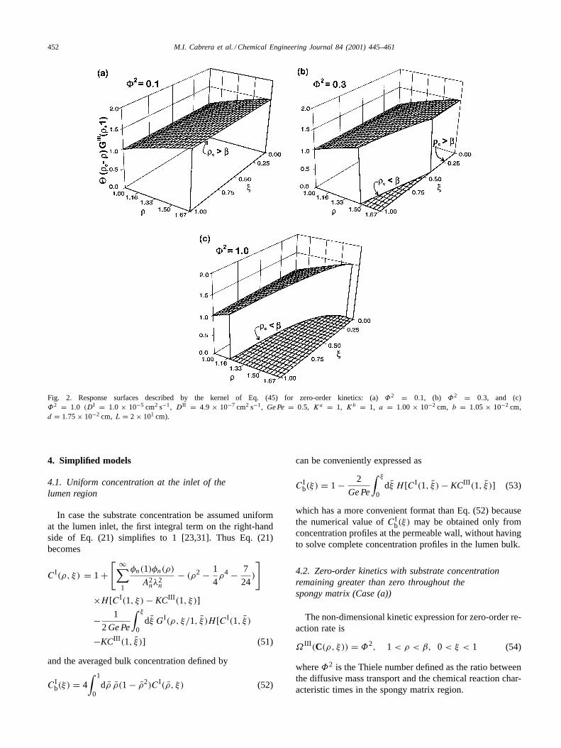
Fig. 2 shows the response surface described by the kernelsof the aforementioned integral equations forρ = 1 andthree values of the Thiele modulus for zero-order kinetics.It may be noticed that the response surface drops to zeroas long as the radial position surpasses the critical radiuswhich is a function of the axial position. It is also evidentthat by increasing the Thiele modulus, the region where theresponse level is zero also increases.


Fig. 2. Response surfaces described by the kernel of Eq. (45) for zero-order kinetics: (a)Φ2 = 0.1, (b) Φ2 = 0.3, and (c)Φ2 = 1.0 (DI = 1.0 × 10−5 cm2 s−1, DII = 4.9 × 10−7 cm2 s−1, Ge Pe = 0.5, Ka = 1, Kb = 1, a = 1.00 × 10−2 cm, b = 1.05 × 10−2 cm,d = 1.75× 10−2 cm, L = 2 × 101 cm).

4. Simplified models

4.1. Uniform concentration at the inlet of thelumen region

In case the substrate concentration be assumed uniformat the lumen inlet, the first integral term on the right-handside of Eq. (21) simplifies to 1 [23,31]. Thus Eq. (21)becomes

CI(ρ, ξ) = 1 +[ ∞∑

1

φn(1)φn(ρ)

A2nλ

2n

− (ρ2 − 1

4ρ4 − 7

24)

]

×H [CI(1, ξ) − KCIII (1, ξ)]

− 1

2Ge Pe

∫ ξ

0dξ GI(ρ, ξ/1, ξ )H [CI(1, ξ )

−KCIII (1, ξ )] (51)

and the averaged bulk concentration defined by

CIb(ξ) = 4

∫ 1

0dρ ρ(1 − ρ2)CI(ρ, ξ) (52)

can be conveniently expressed as

CIb(ξ) = 1 − 2

Ge Pe

∫ ξ

0dξ H [CI(1, ξ ) − KCIII (1, ξ )] (53)

which has a more convenient format than Eq. (52) becausethe numerical value ofCI

b(ξ) may be obtained only fromconcentration profiles at the permeable wall, without havingto solve complete concentration profiles in the lumen bulk.

4.2. Zero-order kinetics with substrate concentrationremaining greater than zero throughout thespongy matrix (Case (a))

The non-dimensional kinetic expression for zero-order re-action rate is

Ω III (C(ρ, ξ)) = Φ2, 1 < ρ < β, 0 < ξ < 1 (54)

whereΦ2 is the Thiele number defined as the ratio betweenthe diffusive mass transport and the chemical reaction char-acteristic times in the spongy matrix region.


By integration of Eq. (44) with Eqs. (50) and (54), weobtain the following explicit expression:

CIII (ρ, ξ) = 1

KCI(1, ξ)

+νΦ2

1

2HK[β2−1]− 1

4[ρ2−1]+ β2

2ln ρ

(55)

from which theCIII (ρ, ξ) profile can be readily obtainedonce theCI(1, ξ) profile is available. From Eq. (55), it imme-diately follows that the impulsive force for the mass transferbetween the lumen and spongy matrix sides is

H [CI(1, ξ) − KCIII (1, ξ)] = −12ν(β

2 − 1)Φ2 (56)

Then, substituting this relationship into Eq. (51), it becomes

CI(ρ, ξ) = 1 + νΦ2β2 − 1

2

ρ2 − 1

4ρ4 − 7

24+ 2

Ge Peξ

−∞∑1

φn(ρ)φn(1)

A2nλ

2n

exp

(− λ2

n

2Ge Peξ

)(57)

from which, forρ = 1, we obtain

CI(1, ξ) = 1 + νΦ2β2 − 1

2

11

24+ 2

Ge Peξ

−∞∑1

φ2n(1)

A2nλ

2n

exp

(− λ2

n

2Ge Peξ

)(58)

The uncoupled Equations (57) and (58) have validity when-ever the substrate concentration at the permeable wall isgreater than the critical concentration for which the concen-tration just depletes at the shell wall, that is whenever thecondition

CI(1, ξ) ≥ −νΦ2

×

1

2H[β2 − 1] − K

4[β2 − 1] + β2K

2ln β

(59)

is satisfied. This result provides a lower bound for thesubstrate concentration at the lumen wall above which theboundary condition given by Eqs. (19a) and (19b) has fullvalidity.

4.3. Zero-order kinetics with substrate depleted beforereaching the shell wall (Case (b))

So long as the reaction rate is zero if the substrate concen-tration drops to zero, the non-dimensional kinetic equationcan be formally expressed as

Ω III (C(ρ, ξ)) = Θ(ρc − ρ)Φ2,

1 < ρ < β, 0 < ξ < 1 (60)

Substitution of Eq. (60) into Eq. (45) followed by integrationusing Eq. (50) gives

CIII (ρ, ξ) = Θ(ρc − 1)1

KCI(1, ξ) + Θ(ρc − ρ)νΦ2

×

1

2HK[ρ2

c − 1] − 1

4[ρ2 − 1] + ρ2

c

2ln ρ

(61)

from which theCI(1, ξ) profile can be easily obtained in-voking the substrate depletion just atρ = ρc, thus:

CI(1, ξ)

= −νΦ2K

1

2HK[ρ2

c −1]− 1

4[ρ2

c −1]+ ρ2c

2ln ρc

(62)

Substitution of Eq. (62) into Eq. (61) leads to a simple equa-tion which describes the substrate concentration profile inthe spongy matrix region:

CIII (ρ, ξ) = Θ(ρc − ρ)νΦ2

1

4[ρ2

c − ρ2] + ρ2c

2ln

ρ

ρc

(63)

whereρc remains still unspecified. Then, from Eqs. (60)–(63)comes out the need for the knowledge of the critical radiusρc.

An additional condition to be satisfied byρc comes fromEq. (55) evaluated atρ = 1:

H [CI(1, ξ) − KCIII (1, ξ)] = −12ν(ρ

2c − 1)Φ2 (64)

Then, substitution of Eq. (64) into Eq. (51), after integration,yields

CI(ρ, ξ) = 1 + νΦ2ρ2c − 1

2

ρ2− 1

4ρ4− 7

24+ 2

Ge Peξ

−∞∑1

φn(ρ)φn(1)

A2nλ

2n

exp

(− λ2

n

2Ge Peξ

)(65)

which for ρ = 1 becomes

CI(1, ξ) = 1 + νΦ2ρ2c − 1

2

11

24+ 2

Ge Peξ

−∞∑1

φ2n(1)

A2nλ

2n

exp

(− λ2

n

2Ge Peξ

)(66)

Finally, by linking Eqs. (62) and (66), it results that

0 = 1 +νΦ2K

1

2HK[ρ2

c − 1] − 1

4[ρ2

c − 1] + ρ2c

2ln ρc

+νΦ2ρ2c − 1

2

11

24+ 2

Ge Peξ

−∞∑1

φ2n(1)

A2nλ

2n

exp

(− λ2

n

2Ge Peξ

)(67)


from which the critical radius can be numerically obtainedas a function of the axial position.

As a limiting case of this generalized formulation, Eq. (67)provides an unmatched expression upon the knowledge ofthe critical radius as a function of the axial position and thediffusive-to-convective (Pe) and diffusive-to-reaction (Φ2)characteristic times ratios, the partitioning parameters (K),the mixed parameters (H ), and the geometrical ratio (Ge)of the HFBR. The values of the critical radius can be ob-tained according to Eq. (67) by application of any standardmethod to solve zeros of a system of nonlinear equations.Then, once the values of the critical radius are known, thesubstrate concentration profiles in the active matrix and lu-men regions can be straightaway obtained from Eqs. (63)and (65), respectively, without having to resort to an itera-tive scheme of numerical solution.

5. Numerical solution

5.1. Numerical algorithm

The concentration profiles of substrate at the membranewall on the lumen side can be obtained from Eq. (26), and onthe spongy matrix from Eq. (44) evaluated atρ = 1. Then theproposed iterative procedure to obtain the solution proceedsas follows: (i) assume values for the concentration profileson the boundary atρ = 1; (ii) solve Eq. (26) according tothe sequence:

CI(1, ξ)j+1 = F [CIII (1, ξ), CI(1, ξ)j ] (68)

until the resulting axial profile has the desired accuracy; (iii)solve Eq. (44) with the result obtained in step (ii) following

Fig. 3. Distribution of the substrate concentration in the lumen and spongy matrix regions: (a) Michaelis–Menten kinetics(Φ2 = 1 andKM = 1 mol cm−3),and (b) zero-order kinetics(Φ2 = 1) (DI = 1.0× 10−5 cm2 s−1, DII = 1.0× 10−6 cm2 s−1, DIII = 1.0× 10−5 cm2 s−1, Ge Pe= 0.125,Ka = 1, Kb = 1,a = 1.00× 10−2 cm, b = 1.05× 10−2 cm, d = 1.75× 10−2 cm, L = 2 × 101 cm).

the sequence:

CIII (ρ, ξ)k+1 = F [CI(1, ξ), CIII (ρ, ξ)k] (69)

until the resulting radial profile has the desired accuracy;(iv) evaluateCIII (1, ξ) from the values obtained in step (iii)and compare with the old profile assumed in step (i); and(v) proceed with the iterative scheme until each value ofCIII (1, ξ) calculated between two consecutive steps of over-all iteration has a relative error smaller than the prescribedvalue. Thus, the iterative process proceeds on the boundaryat ρ = 1 and throughout the spongy matrix, without havingto solve the complete concentration profiles in the lumenregion.

The sequences described by Eqs. (68) and (69) converge ifa Lipzchitz condition is satisfied by both equations [35,36].Convergence is usually obtained for typical values of themodel parameters and for a wide variety of differentiablekinetic equations as will be analyzed below.

For integration purposes, the use of uniform rectangulargrids in theρ, ξ -space is simple, but not suitable for the sim-ulation of HFBRs operating in reaction regimes controlledby the mass diffusion rate, i.e.,Ge Pe< 1 and/orΦ2 > 1. Insuch case, a rapid depletion of the substrate can take placenear the inner tube entrance and/or the membrane wall onthe spongy matrix side, as shown in Fig. 3. Then, if thenumber of grid points is not large enough the numerical in-tegration cannot be sufficiently accurate. However, the useof enough grid points will be prohibitively demanding com-puter memory space and with computation times unaccept-ably large. For example, the total number of grid points usedin ξ -space essentially depends upon the value of the param-eterGe Pe. In Table 1, results obtained with different meshsizes are compared with those accepted as the exact solution,


Table 1Errors relative to the exact solution in terms of theGe Peparameter for different mesh sizesa

Ge Pe Relative error (%)

50 meshes 100 meshes 200 meshes 400 meshes 600 meshes 800 meshes 1000 meshes

(a) Percentage error in predictions of the substrate concentration at the membrane wall on the lumen side atξ = 0.10.50 8.47 5.15 2.97 1.41 0.72 0.29 0.001.00 6.99 4.35 2.53 1.22 0.62 0.27 0.002.00 5.61 3.53 2.06 0.99 0.50 0.20 0.004.00 4.40 2.76 1.58 0.73 0.35 0.14 0.00(b) Percentage error in predictions of the substrate averaged bulk concentration on the lumen side atξ = 0.10.50 0.55 0.05 0.18 0.14 0.08 0.04 0.001.00 0.49 0.10 0.02 0.04 0.03 0.01 0.002.00 0.34 0.10 0.02 0.00 0.00 0.00 0.004.00 0.20 0.07 0.02 0.00 0.00 0.00 0.00

aDI = 1.0 × 10−5 cm2 s−1, DII = 1.0 × 10−6 cm2 s−1, Ge Pe= 0.5, Ka = 1, Kb = 1, H = 2.0, n = 1, a = 1.00× 10−2 cm, b = 1.05× 10−2 cm,d = 1.75× 10−2 cm, L = 2 × 101 cm.

which are achieved with a fixed axial grid containing 1000meshes. It is noticeable that a workable mesh size in a per-sonal computer, for example 200 meshes, only provides anacceptable agreement with the exact solution for values ofGe Pegreater than 1. However, for the same number of gridpoints, non-uniform grids give more accurate results. Thenthe mentioned limitation can be overcome using a contin-uous transformation of theξ -coordinate and the numericalintegration can be done on a uniform rectangular grid inthe transformed space. A similar approach can be applied totransform theρ-coordinate in the spongy matrix region.

5.2. Grid transformations

Several techniques for grid generation and the use thereofin the numerical solution of differential equations have beenproposed to obtain grid points closely spaced in regionswith steep gradients and widely spaced where the changes

Fig. 4. Coordinate transformations for the integral equations governing the species mass balances: (a) in the lumen region, and (b) in the spongy matrixregion.

are smooth [37–39]. We have found that the followingtransformations are quite suitable to solve the derived inte-gral equations:

1. In the lumen region, a newζ -coordinate can be suitablyrelated to the originalξ -coordinate through the followingequation:

ξ = 1 − tanh [(1 − ζ ) tanh−1√1 − αζ ]√1 − αζ

(70)

where 0 ≤ ξ ≤ 1, 0 ≤ ζ ≤ 1, and αζ is an ad-justable parameter ranging between 0 and 1 [37]. Notethat whenαζ is equal to 1, Eq. (70) reduces to the identitytransformationξ = ζ . According to this transformation,uniform mesh sizes inζ -coordinate have grid points inξ -coordinate closely spaced near the entrance of the innertube and widely spaced far from that, as shown in Fig. 4a.

2. In the spongy matrix region, the newϕ-coordinate tobe related with the originalρ-coordinate is given by the


following transformation:

ρ = 1 + β

1 − tanh [(1 − ϕ) tanh−1√1 − αϕ ]√

1 − αϕ

(71)

where 1≤ ρ ≤ β, 1 ≤ ϕ ≤ β, andαϕ is an adjustableparameter ranging between 0 and 1. Ifαϕ is equal to 1,Eq. (71) reduces to the identity transformationρ = ϕ.Unlike the previous choice, this transformation producesa continuous stretching of the mesh size inρ-coordinateat the vicinity of the membrane on the spongy matrixside, as illustrated in Fig. 4b. It is noticeable that thesmaller theαϕ and αζ values become, the higher thestretching results.

5.3. Transformed integral equations

The governing integral equations are now subjected to theproposed transformations. According to the transformationdefined by Eq. (70), Eq. (26) inρ, ζ -space becomes

CI(ρ, ζ ) =[ ∞∑

1

φn(1)φn(ρ)

A2nλ

2n

− (ρ2 − 1

4ρ4 − 7

24)

]

×H [CI(1, ζ ) − KCIII (1, ζ )]

+∫ 1

0dρ ρ(1 − ρ2)GI(ρ, ζ/ρ,0)CI(ρ,0)

− 1

2Ge Pe

∫ ζ

0dζ JζG

I(ρ, ζ/1, ζ )H [CI(1, ζ )

−KCIII (1, ζ )] (72)

then

CI(1, ζ ) =[ ∞∑

1

φ2n(1)

A2nλ

2n

− 11

24

]H [CI(1, ζ ) − KCIII (1, ζ )]

+∫ 1

0dρ ρ(1 − ρ2)GI(1, ζ/ρ,0)CI(ρ,0)

− 1

2Ge Pe

∫ ζ

0dζ JζG

I(1, ζ/1, ζ )H [CI(1, ζ )

−KCIII (1, ζ )], 0 ≤ ζ ≤ 1 and 0≤ ζ ≤ 1

(73)

where the integration is now realized by taking equal in-crements inζ -coordinate, instead ofξ -coordinate, and theJacobianJζ is given by

Jζ = tanh−1√1 − αζ sech2[(1 − ζ ) tanh−1√1 − αζ ]√1 − αζ

(74)

According to Eq. (71), Eq. (44) inϕ, ξ -space becomes

CIII (ϕ, ξ) = GIII (ϕ/1)HCI(1, ξ)

+ν

∫ β

1dϕ JϕϕG

III (ϕ/ϕ)Ω III (C(ϕ, ξ)),

1 ≤ ϕ ≤ β (75)

with

CIII (1, ξ) = GIII (1/1)HCI(1, ξ)

+ν

∫ β

1dϕ JϕϕG

III (1/ϕ)Ω III (C(ϕ, ξ)),

1 ≤ ρ ≤ β (76)

respectively, where the integration is now realized by takingequal increments inϕ-coordinate instead ofρ-coordinate.The JacobianJϕ is given by

Jϕ = β tanh−1√1 − αϕ sech2[(1 − ϕ) tanh−1√1 − αϕ ]√1 − αϕ

(77)

5.4. Numerical exploitation

Eqs. (73) and (76) were solved through the iterative pro-cedure proposed in Section 5.1 until relative errors smallerthan 10−4 were achieved. A simple equispaced quadraturealgorithm, such as the Newton38 method, was used to per-form the numerical integration. All calculations were per-formed in double precision arithmetic.

Fig. 5a and b shows the axial profiles of the substrate con-centration at the membrane wall on the lumen side and theaveraged bulk concentration, both in a region near to the en-trance of the HFBR, for two typical values of the parameterGe Pe. Results obtained by solving Eqs. (73) and (75) witha workable number of mesh points (grids with 200 meshesandαζ = 0.1,0.5 and 1.0) are compared with those whichcan be accepted as the exact solution (fixed grid with 1000meshes). There are significant deviations between the pre-dicted values with a fixed grid with 200 meshes (αζ = 1)and the exact values obtained with 1000 meshes (αζ = 1). Itis apparent that the lower the value ofGe Pe, the greater thedeviations become. Then the computation would be done ona very refined equispaced grid inξ -space. However, the useof grids with more than 250 meshes is not practical sinceachieving the solution requires excessive computational ef-fort and computer memory space. The transformation givenby Eq. (70) allows us to overcome such difficulties. In fact,the continuous variable grid method with 200 meshes andαζ ≤ 1 × 10−1 predicts concentration profiles similar orequal to those which are achieved with 1000 meshes, asshown in Fig. 5a and b. For the case analyzed, the optimalvalue of parameterαζ was found to be around 1×10−1 andessentially depends on the value ofGe Pe. After considerablenumber of attempts, we proposed to chooseαζ according tothe following relationship:

αζ =

1 for Ge Pe≥ 2

0.2Ge Pe for Ge Pe< 2(78)

In the spongy matrix region, the advantages of using thetransformation given by Eq. (71) was corroborated. It wasfound that the simplest choice ofαϕ in terms of the parameter


Fig. 5. Predicted axial profiles: (a) substrate concentration at the membrane wall on the lumen side, and (b) averaged bulk concentration. The profilescorrespond toPe= 400 and 1200,Ge= 5 × 10−4, H = 2, K = 1 andΦ2 = 1. () exact value withαζ = 1 and 1000 meshes; () αζ = 1 and 200meshes; () αζ = 0.5 and 200 meshes; and () αζ = 0.1 and 200 meshes.

of the model which governs the concentration profiles in thisregion is given by

αϕ =

1 forΦ2 ≤ 1

1/Φ2 forΦ2 > 1(79)

6. Applications and performance of thenumerical method

For all calculations presented herein,a = 100, b =105, d = 175, Re≤ 1500, 250≤ Pe ≤ 1200, 10−4 ≤Ge ≤ 10−3, 5 × 10−1 ≤ H ≤ 8, and 10−1 ≤ Φ2 ≤10. This set of values is in accordance with the model as-sumptions and covers typical operating conditions for HF-BRs. In order to fulfil the assumption (i), the length ofthe lumen region flow before the spongy matrix was esti-mated to be less than 1 cm because the parabolic axial ve-locity profile is fully developed for an entrance lengthLe ≤5.75 × 10−2 × 2a Re [40]. The assumption (ii) is fulfilledwhenever the convective transport is two orders of mag-nitude greater than the axial diffusive transport. In mathe-matical terms, it means 2Pe(1 − ρ2) ≥ 102 Ge, which inthe range 0≤ ρ ≤ 0.999 is nearly satisfied forPe ≥ 250and Ge ≤ 10−2. In the practice, it might be that the ra-dial convective transport will be no null. However, it is tobe hoped that the assumption (iii) be acceptable in accor-dance with the fact that the radial convective transport canbe still neglected with respect to the radial diffusive fluxfor upper bounds of the radial Peclet number [9]. Assump-tions (v) and (viii) are made to reduce computational ef-forts, but there are no restrictions other than the usual oneson the dependence of the physical properties. The validityof assumptions (vi), (vii) and (ix) will particularly dependon the permeable membrane and spongy matrix characteris-tics. A comprehensive analysis on this matter can be foundelsewhere [9].

6.1. Power-law kinetics

The more simplified representation for the substrate reac-tion rate is the power-law model

Ω III (C(ρ, ξ)) = Φ2CIII (ρ, ξ)n (80)

where the dimensionless reaction rate is expressed in termsof the Thiele number and the reaction order (n < 0). Partic-ularly, the first-order limit of the Michaelis–Menten kineticshas been typically used to describe enzymatic reaction rates[7,8,41–44].

The performance of the computational method was an-alyzed covering a wide range of operating conditions andreaction orders. For all the values explored, the calculationtimes to achieve a specified accuracy are reduced by almostan order of magnitude if the transformed grid method is usedinstead of a fixed grid in the originalρ, ξ -space. Conver-gence is ensured when the Lipzchitz condition is satisfied.For Eq. (75) with first-order kinetics, the Lipzchitz condi-tion becomes

1

Φ2>

(1 + β)2

2ln(1 + β) + ((1 + β)2 − 1)

(1

2HK− 1

4

)(81)

This means that the convergence is surely obtained whenthe overall rate of the process is controlled by the chem-ical reaction, i.e., when either the diffusional resistance inthe spongy matrix is negligible (Φ2 < 1), the spongy ma-trix is thin (β → small value), the coefficient of mass trans-fer through the membrane or the partition coefficients arehigh (HK > 1). The condition given by Eq. (81) was nu-merically corroborated, as illustrated in Fig. 6a–c. For allanalyzed values ofH andGe Pe> 1, the convergence do-mains (lower-left) are exactly described by Eq. (81) sincethe convergence is governed by Eq. (75). ForGe Pe< 0.25the convergence domains begins to be governed by Eq. (73)for which, unlike Eq. (75), an explicit expression to predict


Fig. 6. Convergence domains (lower-left regions) for power-law kinetics. The border lines correspond to half-order (n = 0.5), first-order (n = 1) andsecond-order (n = 2) kinetics. The dashed lines indicate the limits predicted by the Lipzchitz condition for the first-order kinetics.

the convergence conditions cannot be obtained. The con-vergence domains are then completed by computational ex-perimentation. Likewise, Fig. 6a–c shows the convergencemaps corresponding to half-order and two-order kinetics. Itis noticeable that the convergence domains broaden whenthe membrane resistance is lower and the reaction order ishigher. The convergence domains significantly reduce foroperating conditions leading to a process rate significantlycontrolled by diffusive mass transport in the lumen, mem-brane and spongy matrix regions, but such combination ofconditions is either unusual or undesirable in practical ap-plications because the effectiveness of the HFBR becomesexcessively low.

6.2. Michaelis–Menten kinetics

The kinetics for enzymatic reactions are usually ex-pressed on the basis of the general formulation given byMichaelis–Menten:

Fig. 7. Convergence domains (lower-left regions) for Michaelis–Menten kinetics. The border lines indicate the limits for different values of thec0/KM

parameter.

Ω III (C(ρ, ξ)) = Φ2CIII (ρ, ξ)

1 + (c0/KM)CIII (ρ, ξ)(82)

which resembles that suggested by Langmuir for sur-face catalysis. Significant analyses of HFBRs withMichaelis–Menten kinetics have been published elsewhere[5,8,23,42,45–47].

Fig. 7a–c illustrate the convergence domains for a widerange of values of the kinetic parameters. It is apparent thatthe convergence can be achieved in a domain wider thanthe one obtained for first-order kinetics. In regions close tothe convergence limits, the results have repeatedly shownhigh-gradients of concentration which severely restrict thesubstrate available to the cells, the reaction conditionsbecoming vastly inadequate. From a practical viewpoint,non-convergence domains coincide with unacceptable spec-ifications of the HFBR system. For the most demandingconditions, the computing times obtained with the trans-formed grid method become nearly one order of magni-tude smaller than the corresponding one to fixed grids in


ρ, ξ -space, as mentioned in Section 5.4. The convergencemaps can be used to know a priori the feasibility to imple-ment iterative schemes of sure and fast convergence.

6.3. Zero-order kinetics

Some enzymatic reactions can be approximated aszero-order reactions. While the substrate concentration re-mains finite, the non-dimensional kinetic equation becomesindependent of the concentration:

Ω III (C(ρ, ξ)) = Φ2 (83)

but as long as the substrate concentration drops to zero —at the so-called critical radius — the local reaction rate be-comes zero. Theoretical analysis of HFBRs with zero-orderkinetics as limiting form of the Michaelis–Menten kineticscan be found in several contributions [8,15,41,42].

The values of the critical radius can be obtained as rootsof the following implicit equation:

1 + νΦ2K

1

2HK[ρ2

c − 1] − 1

4[ρ2

c − 1] + ρ2c

2ln ρc

+νΦ2ρ2c − 1

2

×

11

24+ 2

Ge Peξ −

∞∑1

φ2n(1)

A2nλ

2n

exp

(− λ2

n

2Ge Peξ

)

= 0 (84)

which was derived as particular case of Eq. (45). The sub-routine ZSPOW of the IMSL library has proved to be ef-fective to solve Eq. (84). The algorithm is a variation of theNewton method and takes precautions to avoid large stepsizes or increasing residuals [48].

Once the values of the critical radius are known, the con-centration profiles can be obtained without having to resortto an iterative scheme of numerical solution.

Fig. 8. Maps showing the domains (left regions) for which the substrate concentration remains greater than zero everywhere inside the spongy matrixfor zero-order kinetics. The border lines indicate the limits for different values of the lumen/spongy matrix partition coefficient.

Case (a). When the substrate concentration remains greaterthan zero throughout the spongy matrix (i.e., whereρc ≥ β),the following explicit equations must be solved:

CI(ρ, ξ) = 1 + νΦ2β2 − 1

2

ρ2− 1

4ρ4− 7

24+ 2

Ge Peξ

−∞∑1

φn(ρ)φn(1)

A2nλ

2n

exp

(− λ2

n

2Ge Peξ

)(85)

and

CIII (ρ, ξ) = 1

KCI(1, ξ) + νΦ2

×

1

2HK[β2 − 1] − 1

4[ρ2 − 1] + β2

2ln ρ

(86)

Case (b). When the substrate concentration depleted beforereaching the shell wall (i.e., whereρc < β), the followingexplicit equations must be used:

CI(ρ, ξ) = 1 + νΦ2ρ2c − 1

2

ρ2− 1

4ρ4− 7

24+ 2

Ge Peξ

−∞∑1

φn(ρ)φn(1)

A2nλ

2n

exp

(− λ2

n

2Ge Peξ

)(87)

and

CIII (ρ, ξ) = Θ(ρc − ρ)νΦ2

1

4[ρ2

c − ρ2] + ρ2c

2ln

ρ

ρc

(88)

Numerical computations are very fast as corroborated byan extensive numerical exploitation. Nevertheless, it seems


convenient to present maps in terms of the HFBR parame-ters showing if the substrate concentration can be depletedbefore reaching the shell wall, and thus knowing a prioriif Eq. (84) must be solved. Results of numerous computa-tions are shown in Fig. 8a–c on which the operation pointcan be located according to the operating conditions to beanalyzed. If the operation point is located within the corre-sponding dashed region, the substrate concentration remainsgreater than zero everywhere inside the spongy matrix, andthen only Eqs. (85) and (86) must be solved. Otherwise, theaxial profile of the critical radius must be necessarily ob-tained from Eq. (84).

7. Conclusions

A formal general solution of the mass balance equationsfor HFBRs with any arbitrary kinetic equation was obtainedby means of the Green’s function method. The general so-lution is said formal because it is expressed in terms of im-plicit integral equations which require some iterative schemeof solution. The substrate remaining finite throughout thespongy matrix and the substrate exhausted before reachingthe shell wall cases are both treated in systematic form usingan indicator function whose values are one if the substrateconcentration is finite, and zero if the substrate concentra-tion is equal to zero. The obtained general solution rendersexplicit analytical forms for limiting cases, some of themhave been treated in the literature.

The main advantages of the solution for the substrate con-centration lies in the following facts: (i) on the lumen side,Green’s functions are expressed in terms of an eigenvalueproblem which depends neither on the particular conditionsof the laminar flow nor on the coefficients of mass transferthrough the permeable membrane, so that once eigenvaluesare calculated, they become a result which does not varyfrom one application to another; (ii) on the spongy matrixside, Green’s functions do not depend on the kinetic equa-tion, this avoids repetitive computational effort when treat-ing different reaction kinetics; (iii) the resulting format ofintegral equations is apt to devise a numerical solution basedon a simple iterative process along the permeable wall andthrough the spongy matrix, without having to resort to thecomplete concentration profiles in the lumen, which yieldto iterative schemes of fast convergence; and (iv) zero-orderkinetics are treated as a particular case of the general so-lution which lead to an unmatched expression in terms ofthe critical radius and operative parameters of the HFBR,from which it is possible to calculate the critical radius ina fast, direct, reliable manner using the proposed numericalalgorithms. Once the values of the critical radius are known,the substrate concentration profiles in the lumen and spongymatrix can be straightaway obtained from explicit analyticalequations.

The numerical procedure can adequately handle problemswith steep axial and radial gradients of concentration in the

lumen and spongy matrix regions, respectively. In regard toimplementation, an improvement of the accuracy of the so-lution without wasting computer memory space and runningtime was obtained with the transformed grid method usinghyperbolic tangent functions. The method can be extendibleto other continuous transformations by the simple substitu-tion of the corresponding Jacobian expression in Eqs. (72),(73), (75) and (76). Then, the computation can be done on afixed uniform grid using standard techniques of integration.The convergence of the iterative procedure can be achievedfor a wide range of operating conditions having practicalimportance. The results presented herein demonstrate theeffectiveness of this approach for the simulation of HFBRswith power-law, Michaelis–Menten and zero-order kinetics;however it is readily extendible to any arbitrary functionalform of the kinetic equation.

Acknowledgements

Support from the Consejo Nacional de InvestigacionesCientıficas y Técnicas (CONICET) and from the Universi-dad Nacional del Litoral of Argentina is gratefully acknowl-edged.

References

[1] R.A. Knazek, P.M. Guillino, P.O. Kohler, R.L. Dedrick, Cell-cultureon artificial capillaries. Approach to tissue growth in vitro, Science178 (1972) 65.

[2] G. Belfort, Membranes and bioreactors: a technical challenge inbiotechnology, Biotechnol. Bioeng. 33 (1989) 1047–1066.

[3] P.S. Sehanputri, C.G. Hill Jr., Biotechnology for the production ofnutraceuticals enriched in conjugated linoleic acid. I. Uniresponsekinetics of the hydrolysis of corn oil by aPseudomonassp. lipaseimmobilized in hollow fiber reactors, Biotechnol. Bioeng. 64 (5)(1999) 568–579.

[4] J.E. Dowd, I. Weber, B. Rodriguez, J.M. Piret, K.E. Kwok, Predictivecontrol of hollow-fiber bioreactors for the production of monoclonalantibodies, Biotechnol. Bioeng. 63 (4) (1999) 484–492.

[5] J.D. Brotherton, P.C. Chau, Modeling of axial-flow hollow fiber cellculture bioreactors, Biotecnol. Prog. 12 (5) (1996) 575–590.

[6] L.R. Waterland, A.S. Michaels, C.R. Robertson, A theoretical modelfor enzymatic catalysis using asymmetric hollow fiber membranes,AIChE J. 20 (1) (1974) 50–59.

[7] S.S. Kim, D.O. Cooney, An improved theoretical model for hollowfiber enzymatic reactors, Chem. Eng. Sci. 31 (1976) 289–294.

[8] I.A. Webster, M.L. Schuler, Mathematical models for hollow fiberenzyme reactors, Biotech. Bioeng. 20 (10) (1978) 1541–1556.

[9] J.M. Piret, C.L. Cooney, Model of oxygen transport limitations inhollow fiber bioreactors, Biotechnol. Bioeng. 37 (1991) 80–92.

[10] M.E. Davis, J. Yamanis, Analysis of annular bed reactor formethanation of carbon-monoxide, AIChE J. 28 (2) (1982) 266–273.

[11] M.E. Davis, J. Yamanis, Axial dispersion in the annular bed reactor,Chem. Eng. Commun. 25 (1984) 1–10.

[12] H. Beyenal, A. Tanyolaç, A mathematical model for hollow fiberbiofilm reactors, Chem. Eng. J. 56 (1994) B53–B59.

[13] M.E. Davis, L.T. Watson, Mathematical modeling of annular reactors,Chem. Eng. J. 33 (1986) 133–142.

[14] V.K. Jayaraman, The solution of hollow fiber bioreactor designequations, Biotechnol. Prog. 8 (1992) 462–464.


[15] V.K. Jayaraman, Solution of hollow fiber bioreactor design equationsfor zero-order limit of Michaelis–Menten kinetics, Chem. Eng. J. 51(1993) B63–B66.

[16] V.K. Jayaraman, Solution of hollow fiber bioreactor design equations:the case of power-law fluids, Chem. Eng. J. 55 (1994) B73–B75.

[17] R.N. Paunovic, Z.Z. Zavargo, M.N. Tekic, Analysis of a model ofhollow-fiber bioreactor wastewater treatment, Chem. Eng. Sci. 48 (6)(1993) 1069–1075.

[18] C. Kleinstreuer, S.S. Agarwal, Analysis and simulation ofhollow-fiber bioreactor dynamics, Biotechnol. Bioeng. 28 (1986)1233–1240.

[19] J. Koska, B.D. Bowen, J.M. Piret, Protein transport in packed-bedultrafiltration hollow-fibre bioreactors, Chem. Eng. Sci. 52 (14)(1997) 2251–2263.

[20] R.A. Kumar, J.M. Modak, Transient analysis of mammalian cellgrowth in hollow fibre bioreactors, Chem. Eng. Sci. 52 (12) (1997)1845–1860.

[21] D.G. Taylor, J.M. Piret, B.D. Bowen, Protein polarization in isotropicmembrane hollow-fiber bioreactors, AIChE J. 40 (2) (1994) 321–333.

[22] C. Heath, G. Belfort, Immobilization of suspended mammalian cells:analysis of hollow fiber and microcapsule bioreactors, Adv. Biochem.Eng./Biotechnol. 34 (1987) 1–31.

[23] R.J. Grau, A.E. Cassano, H.A. Irazoqui, Mass transfer throughpermeable walls: a new integral equation approach for cylindricaltubes with laminar flow, Chem. Eng. Commun. 64 (1988) 47–65.

[24] P. Arce, An integral-spectral formulation for convective–diffusivetransport in a packed-bed with adsorption at the wall and bulkreaction, Chem. Eng. Commun. 138 (1995) 113–125.

[25] R.J. Grau, M.I. Cabrera, A.E. Cassano, The laminar flow tubularreactor with homogeneous and heterogeneous reactions. I. Integralequations for diverse reaction rate regimes, Chem. Eng. Commun.,in press.

[26] M.I. Cabrera, R.J. Grau, A.E. Cassano, The laminar flowtubular reactor with homogeneous and heterogeneous reactions. II.Application to reactor modeling involving free radical reactions,Chem. Eng. Commun., in press.

[27] H. Cantero, R.J. Grau, M.A. Baltanás, Cocurrent turbulent tubereactor with multiple gas injections and recycle of slurry: a treatmentin terms of Green’s functions, Comput. Chem. Eng. 18 (7) (1994)551–561.

[28] P. Arce, B.R. Locke, I.M.B. Trigatti, An integral-spectral approachfor reacting Poiseuille flows, AIChE J. 42 (1) (1996) 23–41.

[29] Z. Chen, P. Arce, B.R. Locke, Convective–diffusive transport with awall reaction in Couette flows, Chem. Eng. J. 61 (1996) 63–71.

[30] Z. Chen, P. Arce, An integral-spectral approach for convective–diffusive mass transfer with chemical reaction in Couette flow.

Mathematical formulation and numerical illustration, Chem. Eng. J.68 (1997) 11–27.

[31] P.E. Arce, A.E. Cassano, H.A. Irazoqui, The tubular reactor withlaminar flow regime: an integral equation approach. I. Homogeneousreaction with arbitrary kinetics, Comput. Chem. Eng. 12 (11) (1988)1103–1113.

[32] M. Abramowitz, I.A. Stegun, Handbook of Mathematical Functions,Dover, New York, 1965.

[33] P.A. Dirac, The Principles of Quantum Mechanics, 4th Edition,Oxford University Press, Oxford, 1958.

[34] B. Tabis, A method of calculation for tubular reactors using a Green’sfunction, Int. Chem. Eng. 27 (1987) 539–544.

[35] E.A. Coddington, N. Levinson, Theory of Ordinary DifferentialEquations, McGraw-Hill, New York, 1955.

[36] M. Guzman, Real Variable Methods in Fourier Analysis,North-Holland, Amsterdam, 1981.

[37] A.K. Agrawal, R.S. Peckover, Nonuniform grid generation forboundary-layer problems, Comput. Phys. Commun. 19 (1980) 171–178.

[38] E. Kalnay de Rivas, On the use of nonuniform grids infinite-difference equations, Comput. Phys. Commun. 10 (1972) 202–210.

[39] J.F. Thompson, Z.U.A. Warsi, C.W. Mastin, Numerical GridGeneration. Foundations and Applications, Elsevier, New York, 1985.

[40] H.L. Langhaar, Trans. Am. Soc. Mech. Eng. A 64 (1942) 55.[41] P.R. Rony, Multiphase catalysts. 2. Hollow fiber catalysts, Biotech.

Bioeng 13 (3) (1971) 431.[42] I.A. Webster, M.L. Schuler, Whole-cell hollow-fiber reactor. Transient

substrate concentration profiles, Biotech. Bioeng. 23 (2) (1981) 447–450.

[43] J.A. Schoenberg, G. Belfort, Enhanced nutrient transport in hollowfiber perfusion reactor, Biotech. Prog. 3 (1987) 80–89.

[44] R. Willaert, A. Smets, L. De Vuyst, Mass transfer limitationsin diffusion-limited isotropic hollow fiber bioreactors, Biotechnol.Technol. 13 (5) (1999) 317–323.

[45] C. Horvath, L.H. Shendalwan, R.T. Light, Open tubularheterogeneous enzyme reactors. Analysis of a theoretical model,Chem. Eng. Sci. 28 (2) (1973) 375–388.

[46] C. Georgakis, P.C.H. Chan, R. Aris, Design of stirred reactorswith hollow fiber catalysts for Michaeles–Menten kinetics, Biotech.Bioeng. 17 (2) (1975) 99.

[47] S.A. Benner, Enzyme kinetics and molecular evolution, Chem. Rev.89 (1989) 789–806.

[48] J. More, B. Garbow, K. Hillstromn, Used Guide for MINPACK-1,Argonne National Laboratory Report ANL-80-74, Argonne, IL,August, 1980.

solving design equations for a hollow fiber bioreactor with arbitrary kinetics

Documents