solutions to homework assignment 2 warm-up...

Biostatistics 201A Homework Solutions 2

October 2nd, 2011

Solutions To Homework Assignment 2

Warm-Up Problems

(1) ANOVA Basics:

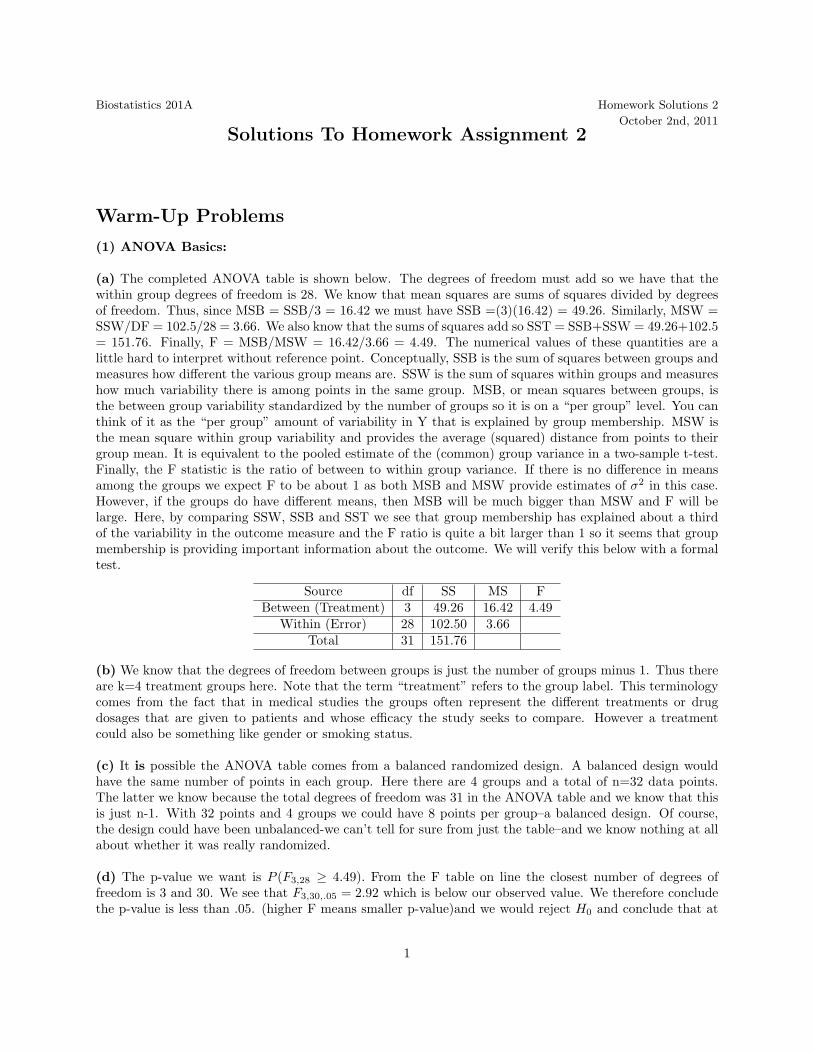
(a) The completed ANOVA table is shown below. The degrees of freedom must add so we have that thewithin group degrees of freedom is 28. We know that mean squares are sums of squares divided by degreesof freedom. Thus, since MSB = SSB/3 = 16.42 we must have SSB =(3)(16.42) = 49.26. Similarly, MSW =SSW/DF = 102.5/28 = 3.66. We also know that the sums of squares add so SST = SSB+SSW = 49.26+102.5= 151.76. Finally, F = MSB/MSW = 16.42/3.66 = 4.49. The numerical values of these quantities are alittle hard to interpret without reference point. Conceptually, SSB is the sum of squares between groups andmeasures how different the various group means are. SSW is the sum of squares within groups and measureshow much variability there is among points in the same group. MSB, or mean squares between groups, isthe between group variability standardized by the number of groups so it is on a “per group” level. You canthink of it as the “per group” amount of variability in Y that is explained by group membership. MSW isthe mean square within group variability and provides the average (squared) distance from points to theirgroup mean. It is equivalent to the pooled estimate of the (common) group variance in a two-sample t-test.Finally, the F statistic is the ratio of between to within group variance. If there is no difference in meansamong the groups we expect F to be about 1 as both MSB and MSW provide estimates of σ2 in this case.However, if the groups do have different means, then MSB will be much bigger than MSW and F will belarge. Here, by comparing SSW, SSB and SST we see that group membership has explained about a thirdof the variability in the outcome measure and the F ratio is quite a bit larger than 1 so it seems that groupmembership is providing important information about the outcome. We will verify this below with a formaltest.

Source df SS MS FBetween (Treatment) 3 49.26 16.42 4.49

Within (Error) 28 102.50 3.66Total 31 151.76

(b) We know that the degrees of freedom between groups is just the number of groups minus 1. Thus thereare k=4 treatment groups here. Note that the term “treatment” refers to the group label. This terminologycomes from the fact that in medical studies the groups often represent the different treatments or drugdosages that are given to patients and whose efficacy the study seeks to compare. However a treatmentcould also be something like gender or smoking status.

(c) It is possible the ANOVA table comes from a balanced randomized design. A balanced design wouldhave the same number of points in each group. Here there are 4 groups and a total of n=32 data points.The latter we know because the total degrees of freedom was 31 in the ANOVA table and we know that thisis just n-1. With 32 points and 4 groups we could have 8 points per group–a balanced design. Of course,the design could have been unbalanced-we can’t tell for sure from just the table–and we know nothing at allabout whether it was really randomized.

(d) The p-value we want is P (F3,28 ≥ 4.49). From the F table on line the closest number of degrees offreedom is 3 and 30. We see that F3,30,.05 = 2.92 which is below our observed value. We therefore concludethe p-value is less than .05. (higher F means smaller p-value)and we would reject H0 and conclude that at

1

least some of the means in this problem (whatever it is about!) are different. If we wanted to use STATA toget the exact p-value we would type

display Ftail(3,28,4.49)

“Ftail” tells STATA to give us the probability of being bigger than the value indicated. The first two num-bers in parentheses are the degrees of freedom and the final number is the F statistic. The resulting p-valueis .01077.

(2) Protein Intake:

(a) Our hypotheses are

H0 : µSTD = µLAC = µV EG–the mean protein intake is the same on all three diets.HA : At least two µ’s are different–mean protein intake is different for at least two of the diets.

To perform the test we need to get the F statistic which involves computing the ANOVA table by hand. Wehave k=3 groups and n=26 data points total so the degrees of freedom are k-1=2, n-k = 23 and n-1=25. Toget the sums of squares we note that

SSB =k∑

j=1

nj Y2j −

(∑

Yij)2

n= 10(75)2 + 10(57)2 + 6(47)2 − (10 ∗ 75 + 10 ∗ 57 + 6 ∗ 47)2

26= 3286.15

SSW =k∑

j=1

(nj − 1)s2j = 9(9)2 + 9(13)2 + 5(17)2 = 3695

From this we can compute the mean squares

MSB =SSB

G− 1=

3286.152

= 1643.08

MSW =SSW

n−G=

369523

= 160.65

And finally F:

F =MSB

MSW=

1643.08160.65

= 10.23

Our p-value is the probability of observing an F larger than this, namely P (F2,23 ≥ 10.23). From moreextensive F tables than what I handed out in class we could see that F2,20,.999 = 9.95 and F2,30,.999 = 8.77.Since our F is bigger than both of these values we can be sure that our p-value us less than .001. From thetable on line all you can conclude is that the p-value is less than .05. Using STATA (display Ftail(2,23,10,23))gives an exact p-value of .0006635 which is indeed less than .001. Either way at α = .05 we reject the nullhypothesis and conclude that the diets do not all have the same protein intake. Of course the interestingquestion is which one(s) are different which we explore in the subsequent parts.

(b) We need 95% CIs for each of the means. The standard error for each of our means will be√

MSW/nj

and the associated degrees of freedom are n-k = 23. (We can use the pooled estimate of the variance eventhough we are only dealing with one group. The groups are all assumed to have common variance/standarddeviation and using all the data points gives us the most accurate estimate plus more degrees of freedom.)

2

We will use a t-distribution since we have to estimate the standard deviation. For 95% CIs we thus needt.025,23 = 2.069. For the STD and LAC groups with 10 subjects each the standard error is

√160.56/10 = 4.01

and for the VEG group it is√

160.65/6 = 5.17. The resulting intervals are

STD: 75± (2.069)(4.01) or [66.7,83.3]STD: 57± (2.069)(4.01) or [48.7,65.3]STD: 47± (2.069)(5.17) or [36.3,57.7]

Note that from these intervals (which are NOT adjusted for multiple testing which we will learn about soon)it appears that the mean protein intake on the standard diet is higher than that on either of the other twogroups–the CIs do not overlap. However the CIs for the two vegetarian diets do overlap so we can not besure their protein intake differs.

(c) Using the test for the differences is actually more accurate than just checking of the intervals overlapsince it adjusts properly for the fact that we are testing two groups in the calculation of the standard error.The basic formula for the CI is

Y1 − Y2 ± tα/2,n−G

√MSW (

1n1

+1n2

)

We have the same t value as before–we just need new standard errors. For comparing STD and LAC, bothgroups have 10 subjects so our standard error is

√160.65(.1 + .1) = 5.67. For the other two comparisons we

have one group of 10 and one group of 6 so the standard error is√

160.65(.1 + .167) = 6.55. The resultingintervals are

STD vs LAC: 75− 57± (2.069)(5.67) or [6.27, 29.73]STD vs VEG: 75− 47± (2.069)(6.55) or [14.44, 41.55]STD vs LAC: 57− 47± (2.069)(6.55) or [-3.55, 23.55]

The two intervals involving the standard diet are entirely above 0, meaning we can be sure that the proteinintake is higher on the standard diet than on either of the two vegetarian diets. In particular it is between 6.27and 29.73 units higher than the lacto-ovo diet and 14.44 to 41.55 units higher than the strict vegetarian diet.However the CI for the difference between the two vegetarian diets includes 0 so we do not have sufficient ev-idence to say that the protein intake on these two diets is different. Our best guess is that the protein intakeis 10 units higher on the lacto-ovo diet than on the strict diet but we can not be 95% sure there is a difference.

To do hypothesis tests we take the difference in means and divide by the standard errors. I will write outthe full details for the first test. The others are similar.

H0 : µSTD = µLAC–the protein intakes on the standard and lacto-ovo diets are the same.

HA : µSTD 6= µLAC–the protein intakes on the standard and lacto-ovo diets are not the same.

Note that µSTD = µLAC is equivalent to µSTD −µLAC = 0 so this is the value we use in computing our teststatistic:

tobs =(YSTD − YLAC)− 0√MSW ( 1

nST D+ 1

nLAC)

=18

5.67= 3.17

The correpsonding p-value is 2P (t23 ≥ 3.17) = .0042. Note that we could have approximated this as between.001 and .005 by looking in row for 23 degrees of freedom on the t-table. However I got the exact p-value

3

by typing “display ttail(23,3.17)” in STATA and then doubling the resulting probability. Of course, if I hadhad the original data I could have performed the whole test in STATA and gotten the p-value that way.Since this p-value is smaller than α = .05 we reject the null hypothesis and conclude there is a difference inprotein intake between the standard and lacto-ovo diets.

For the test of STD versus VEG the t-statistic is tobs = 28/6.55 = 4.27 and the correpsonding 2-tailedp-value is (from STATA) .00028.

For the test of LAC versus VEG the t statistic is tobs = 10/6.55 = 1.53 and the corresponding 2-tailedp-value is (from STATA) .14. Based on these p-values we conclude that there is a significant differencebetween the standard and strict diets but we do not have sufficient evidence to show that the lacto-ovo andstrict vegetarian diets have different average protein intakes.

(d) We want to compare the mean of the standard diet with the average of the means of the two vegetariandiets. Thus our contrast is

L = µSTD − µLAC + µV EG

2The constants for the contrast are c1 = 1, c2 = c3 = −.5. Note that this is indeed a contrast since theconstants sum to 0. Our best estimate of the contrast is

L = YSTD − .5YLAC − .5YV EG = 75− .5(57)− .5(47) = 23

The standard error associated with the contrast is√√√√MSW∑

j

c2j

nj=

√160.65(

110

+(.5)2

10+

(.5)2

6) = 5.17

To get a 95% confidence interval we use t.025,23 = 2.069 as above, which gives is 23 ± (2.069)(5.17) or aninterval of [12.30,33.70]. Since this interval is entirely above 0 we conclude that the protein on the standarddiet is higher than the average intake on the two vegetarian diets. Given that the standard diet had asignificantly higher protein intake than both vegetarian diets this is hardly a surprise! If we wanted to do aformal test our hypotheses would be

H0 : L = 0, µSTD = (µLAC + µV EG)/2–the protein intake for the standard diet is the same as the averageof the two vegetarian diets.

HA : L 6= 0, µSTD 6= (µLAC + µV EG)/2–the protein intake for the standard diet is not the same as theaverage of the two vegetarian diets.

The correpsonding test statistic is

tobs =L√

MSW∑ c2

j

nj

=23

5.17= 4.45

The corresponding 2-sided p-value from STATA is .000182 (“display ttail(23,4.45)” and double STATA’svalue.) Since this p-value is very small we conclude that the mean protein intake on the standard diet isdifferent from the average of the vegetarian diets.

(3) Birthweight and Smoking:

4

(a) To find the solution by hand we need to compute the group means and variances. For Group 1 the meanis

Y1 =7.5 + 6.2 + 6.9 + 7.4 + 9.2 + 8.3 + 7.6

7= 7.586

Similar calculations give Y2 = 7.2400, Y3 = 6.3286, Y4 = 6.0125. For the sample variance of Group 1 we get

s21 =

16[(7.5− 7.586)2 + (6.2− 7.586)2 + · · ·+ (7.6− 7.586)2] = .9245

Similar calculations give s22 = .8330, s2

3 = 1.299, s24 = .51839. We can verify this in STATA off the oneway

printout below with the tabulate option. Note that STATA gives the standard deviations of the groups sowe have to square them to get the variances. In SAS you can get the means and standard deviations as partof the printout by using the means statement. Alternatively you could get these values using the summarizecommand with the by option in STATA or proc univariate in SAS as in homework 1.

With these numbers we can compute the values in the ANOVA table:

SSB =k∑

j=1

nj Y2j −

(∑

Yij)2

n

= 7(7.5857)2+5(7.2400)2+7(6.3286)2+8(6, 0125)2− (7(7.5857) + 5(7.2400) + 7(6.3286) + 8(6.0125))2

27= 11.67

SSW =k∑

j=1

(nj − 1)s2j = 6(.9245) + 4(.8330) + 6(1.299) + 7(.5184) = 20.30

From this we can compute the mean squares

MSB =SSB

k − 1=

11.673

= 3.89

MSW =SSW

n− k=

20.3023

= .88

And finally F:

F =MSB

MSW=

3.89.88

= 4.41

For the test our hypotheses are

H0 : µ1 = µ2 = µ3 = µ4–The mean birthweight is the same in the four groups. Smoking status does not im-pact birthweight. HA: At least two of the µj ’s are different. Smoking status does impact average birthweight.

The corresponding STATA and SAS printouts are below. We see that the F statistic is 4.41 matching ourhand calculations and the corresponding p-value is .0137 so at α = .05 we reject the null hypothesis andconclude that there is a difference in average birthweight among the smoking groups.

5

IN STATA:

. oneway birthweight group, tabulate

| Summary of birthweightgroup | Mean Std. Dev. Freq.

------------+------------------------------------1 | 7.5857143 .96164542 72 | 7.2400001 .91268825 53 | 6.3285714 1.1397578 74 | 6.0125 .71999501 8

------------+------------------------------------Total | 6.7296296 1.1089894 27

Analysis of VarianceSource SS df MS F Prob > F

------------------------------------------------------------------------Between groups 11.6726896 3 3.89089655 4.41 0.0137Within groups 20.303607 23 .882765523------------------------------------------------------------------------

Total 31.9762967 26 1.22985756

IN SAS:

proc anova data=work.hw2;class group;model birthweight = group;means group;run;

The ANOVA ProcedureDependent Variable: birthweight

Sum ofSource DF Squares Mean Square F Value Pr > F

Model 3 11.67268915 3.89089638 4.41 0.0137

Error 23 20.30360714 0.88276553

Corrected Total 26 31.97629630

R-Square Coeff Var Root MSE birthweight Mean

0.365042 13.96148 0.939556 6.729630

Source DF Anova SS Mean Square F Value Pr > F

group 3 11.67268915 3.89089638 4.41 0.0137

6

Level of ---------birthweight---------group N Mean Std Dev

1 7 7.58571429 0.961645422 5 7.24000000 0.912688343 7 6.32857143 1.139757704 8 6.01250000 0.71999504

(b) I will do the test comparing the non-smoking and exsmoking groups in detail. The others work the sameway.

H0 : µNS = µEX–the average birthweights of babies born to mothers who never smoked and mothers whono longer smoke are the same.H0 : µNS 6= µEX–the average birthweights of babies born to mothers who never smoked and mothers whono longer smoke are not the same.

Note that µNS = µEX is equivalent to µNS − µEX = 0 so this is the value we use in computing our teststatistic:

tobs =(YNS − YEX)− 0√MSW ( 1

nNS+ 1

nEX)

=.346√

.882( 17 + 1

5 )= .63

The corresponding p-value is 2P (t23 ≥ .63) = .535. I got this using the ttail command and doubling theresult. Since this p-value is huge, we fail to reject the null hypothesis. We have insufficient evidence to con-clude that the babies of mothers who have never smoked and those of ex-smokers have different birthweights.I perform the rest of the tests in STATA using the anova command followed by the test command and in SASusing proc glm. The output is below. Note that STATA and SAS report these as F tests rather than t-testsbut the F statistic is equivalent to the square of the t-statistic and the p-values are the same. Using thep-values from the results below we see that at the α = .05 level we can not say that the NS and EX groupsare different. However the NS group is significantly different from the LOW and HIGH smoking groups. Wehave insufficient evidence to say the EX and LOW smoking groups have different average birthweights, butthe EX and HIGH groups are significantly different. Finally, we see that there is insufficient evidence to saythe LOW and HIGH smoking mothers have babies with different birthweights.

IN STATA:

anova birthweight group

Number of obs = 27 R-squared = 0.3650Root MSE = .939556 Adj R-squared = 0.2822

Source | Partial SS df MS F Prob > F-----------+----------------------------------------------------

Model | 11.6726896 3 3.89089655 4.41 0.0137

7

|Group | 11.6726896 3 3.89089655 4.41 0.0137

|Residual | 20.303607 23 .882765523

-----------+----------------------------------------------------Total | 31.9762967 26 1.22985756

. test 1.group = 2.group

( 1) group[1] - group[2] = 0

F( 1, 23) = 0.39Prob > F = 0.5359


( 1) group[1] - group[3] = 0

F( 1, 23) = 6.27Prob > F = 0.0199


( 1) group[1] - group[4] = 0

F( 1, 23) = 10.47Prob > F = 0.0037


( 1) group[2] - group[3] = 0

F( 1, 23) = 2.74Prob > F = 0.1112


( 1) group[2] - group[4] = 0

F( 1, 23) = 5.25Prob > F = 0.0314


( 1) group[3] - group[4] = 0

8

F( 1, 23) = 0.42Prob > F = 0.5221

Note: In STATA version 9/10 the command and output for the first test would be:

. test _b[group[1]] = _b[group[2]]

( 1) group[1] - group[2] = 0

F( 1, 23) = 0.39Prob > F = 0.5359

and the others would be similar.

IN SAS:

To get contrasts in SAS we use proc glm instead of proc anova but thestructure and interpretation of output is the same:

proc glm data=work.hw2;class group;model birthweight = group;contrast "Group 1 vs Group 2" group 1 -1 0 0;contrast "Group 1 vs Group 3" group 1 0 -1 0;contrast "Group 1 vs Group 4" group 1 0 0 -1;contrast "Group 2 vs Group 3" group 0 1 -1 0;contrast "Group 2 vs Group 4" group 0 1 0 -1;contrast "Group 3 vs Group 4" group 0 0 1 -1;run;

The GLM ProcedureDependent Variable: birthweight


Model 3 11.67268915 3.89089638 4.41 0.0137

Error 23 20.30360714 0.88276553



0.365042 13.96148 0.939556 6.729630

Source DF Type I SS Mean Square F Value Pr > F

group 3 11.67268915 3.89089638 4.41 0.0137

9

Contrast DF Contrast SS Mean Square F Value Pr > F

Group 1 vs Group 2 1 0.34859524 0.34859524 0.39 0.5359Group 1 vs Group 3 1 5.53142857 5.53142857 6.27 0.0199Group 1 vs Group 4 1 9.24001190 9.24001190 10.47 0.0037Group 2 vs Group 3 1 2.42288095 2.42288095 2.74 0.1112Group 2 vs Group 4 1 4.63617308 4.63617308 5.25 0.0314Group 3 vs Group 4 1 0.37296429 0.37296429 0.42 0.5221

(c) We want to test

µNS + µEX

2=

µLOW + µHIGH

2or equivalently

µNS + µEX

2− µLOW + µHIGH

2= 0

This is a contrast with c1 = c2 = .5 and c3 = c4 = −.5. Our estimated value of the contrast is

L = .5YNS + .5YEX − .5YLOW − .5YHIGH = .5(7.59) + .5(7.24)− .5(6.33)− .5(6.01) = 1.245

The standard error associated with the contrast is√√√√MSW∑

j

c2j

nj=

√.8828(

(.5)2

7+

(.5)2

5+

(−.5)2

7+

(−.5)2

8) = .367

We as before use t.025,23 = 2.069 which yields a confidence interval of 1.245 ± (2.069)(.391) or [.44, 2.05].SInce this interval is entirely above 0 we conclude that the average birthweight of the babies born to mothersnot currently smoking is greater than that of babies born to mothers who are currently smoking, specificallyby between .45 and 2.05 pounds. If we wanted to do this as an hypothesis test our test statistic would be

tobs =1.245.367

= 3.39

The corresponding p-value is 2P (t23 ≥ 3.39) = .0026. This leads us to reject the null hypothesis and concludethat babies with currently non-smoking mothers have different average birthweights than those of currentlysmoking mothers. The corresponding STATA and SAS tests are

IN STATA

. test .5*(1.group + 2.group) - .5*(3.group + 4.group)

( 1) .5 group[1] + .5 group[2] - .5 group[3] - .5 group[4] = 0

F( 1, 23) = 11.45Prob > F = 0.0026

10

Note: In STATA versions 9/10 the command and output would be

. test .5*(_b[group[1]] + _b[group[2]]) = .5*(_b[group[3]] + _b[group[4]])

( 1) .5 group[1] + .5 group[2] - .5 group[3] - .5 group[4] = 0

F( 1, 23) = 11.45Prob > F = 0.0026

In SAS:

proc glm data=work.hw2;class group;model birthweight = group;contrast "Group 1+2 vs 3+4" group .5 .5 -.5 -.5;run;

The GLM Procedure

Dependent Variable: birthweight


Model 3 11.67268915 3.89089638 4.41 0.0137

Error 23 20.30360714 0.88276553



0.365042 13.96148 0.939556 6.729630


group 3 11.67268915 3.89089638 4.41 0.0137

Source DF Type III SS Mean Square F Value Pr > F

group 3 11.67268915 3.89089638 4.41 0.0137


Group 1+2 vs 3+4 1 10.10857331 10.10857331 11.45 0.0026

11

(4) Health Is Where the HAART Is:

(a) To determine whether the mean log10 viral load differs across treatment groups we use the F test in anANOVA. We have four treatment groups, N, A, B and AB. The corresponding hypotheses are:

H0 : µN = µA = µB = µAB-there is no difference in average viral load among the four treatment groups. Inother words what treatment you get has nothing to do with your outcome.HA : not all µi are the same. Viral load is related to which treatment a subject receives.

Below are STATA and SAS printouts for the ANOVA. The p-value for the F test is 0 to as many decimal placesas the packages report so it is certainly less than our standard significance level of α = .05. We thereforereject the null hypothesis and conclude that there is a relationship between viral load and which treatmenta subject receives. In fact, since this was a randomized study, we can conclude that the relationship iscausal–that the different treatments have different effects on viral load. The reason you can infer causality ina randomized trial is that all the treatment groups should be the same in terms of every possible confoundingfactor.

IN STATA:

. oneway vload haart, tabulate

| Summary of VloadHaart | Mean Std. Dev. Freq.

------------+------------------------------------1 | 4.6157984 .91861188 312 | 4.2090148 .60964525 313 | 3.9325628 .55513908 314 | 3.2174304 .26721547 31

------------+------------------------------------Total | 3.9937016 .80689927 124


------------------------------------------------------------------------Between groups 32.2306727 3 10.7435576 26.94 0.0000Within groups 47.8529587 120 .398774656------------------------------------------------------------------------

Total 80.0836314 123 .651086434

IN SAS:

The ANOVA Procedure

Dependent Variable: vload vload


Model 3 32.23067451 10.74355817 26.94 <.0001

Error 120 47.85296044 0.39877467

12


R-Square Coeff Var Root MSE vload Mean

0.402463 15.81205 0.631486 3.993702


haart 3 32.23067451 10.74355817 26.94 <.0001

(b) We have four groups so there are 6 possible pairs of means to compare. I will do the comparison of theN and A groups by hand. The rest are completely analogous. The hypotheses we are interested in testing are

H0 : µN = µA or µN − µA = 0–there is no difference in viral load between people who receive no treatmentand those who receive HAART A.HA : µN 6= µA or µN − µA 6= 0–there is a difference in viral loads between people on these two regimens.

The test statistic for a difference of means in an ANOVA is given by

tobs =(YN − YA)− 0√MSW ( 1

nN+ 1

NA)

=4.616− 4.209√.399( 1

31 + 131 )

= 2.54

I got the group means and the value of MSW from the printouts in part (a). As noted previously weuse MSW, the pooled estimate of variance based on ALL the groups even though we are only comparingtwo of them. Since all the groups are asusmed to have the same variance, this is the best esimtate andalso improves our degrees of freedom. Specifically, under the null hypothesis, tobs has a t distribution withn − k = 124 − 4 = 120 degrees of freedom. The corresponding p-value (two-sided since we are just testingwhether the groups are different) is

p− value = 2P (t120 ≥ 2.54) = 2(.0062) = .0124

I got this exact p-value from STATA using the ttail command which gives the probability of being greaterthan 2.54 and then doubling the result. Since this p-value is less than α = .05 we conclude that there isa significant difference in viral loads between subjects receiving no HAART treatment and those receivingHAART A.

. display ttail(120, 2.54)

.00618123

The printouts for the remaining comparisons are shown below. In STATA you can use either the testcommand or the lincom command following the anova command (they don’t work after the oneway commandshown in part (a) so I had to rerun it. I used oneway in (a) to get the summary statistics.) In SAS youuse contrasts as part of proc glm. I have included all the SAS printouts for the rest of this problem at thevery end for efficiency as they can be done as part of a single proc statement. I included all 6 tests forcompleteness. Note that STATA and SAS give the results as F tests rather than t-tests. The F statistic isjust the square of the t-statistic as you can see by squaring our t value of 2.54 for the N vs A test to get6.43, the F statistic for the first test shown below. All these comparisons are significant at the (unadjusted)significance level of α = .05 except the comparison of the second and third groups which correspond to theHAART A alone and HAART B alone groups. We can not be 95% sure there is a difference in viral loadbetween these two treatment groups.

13

IN STATA:

. test 1.haart = 2.haart

( 1) 1b.haart - 2.haart = 0

F( 1, 120) = 6.43Prob > F = 0.0125



F( 1, 120) = 18.14Prob > F = 0.0000



F( 1, 120) = 76.01Prob > F = 0.0000


( 1) 2.haart - 3.haart = 0

F( 1, 120) = 2.97Prob > F = 0.0874


( 1) 2.haart - 4.haart = 0

F( 1, 120) = 38.22Prob > F = 0.0000


( 1) 3.haart - 4.haart = 0

F( 1, 120) = 19.88Prob > F = 0.0000

(c) First we want to see whether patients who are taking HAART A have lower viral loads than those nottaking HAART A. Since the statement said it did not matter whether the subjects were taking HAART Bor not we need to compare the A and AB groups (who are taking A) with the N and B groups (who arenot). Intuitively what we want to show is that the average of the first two groups is less than the average ofthe second two groups:

µA + µAB

2≤ µN + µB

2

14

To turn this into a linear combination we need to bring all the terms over to one side so that we have anexpression for the difference between the two groups we want to compare:

LC =µN + µB

2− µN + µB

2Note that the linear combination does not havea value attached to it–it is just the function of the means weare interested in. I chose to take the non-A group minus the A group so that the difference would come outpositive if the professor’s theory was correct but this is an arbitrary choice.

The best estimate of the effect of HAART A is obtained by plugging in the sample means to the linearcombination:

LC = .5 ∗ (YN + YB)− .5 ∗ (YA + YAB) = .5 ∗ (4.616 + 3.933)− .5 ∗ (4.209 + 3.217) = .5616

In other words the average log 10 viral load of those not taking HAART A is .5616 higher than for thosewho are taking HAART A. In terms of this linear combination the hypotheses for my test are

H0 : LC ≤ 0-those who do not take HAART A have the same or lower viral loads than those who do takeHAART A.HA : LC > 0-those who do not take HAART A have higher viral loads than those who do take HAART A orequivalently those who take HAART A have lower viral loads than those who do not. This is our alternativehypothesis because it is what the professor is trying to prove.

We can get the p-value for this test using the test command in STATA or a contrast subcommand in SAS.The corresponding printouts are shown below. We see that the p-value for the 2-sided test is 0 to 4 decimalplaces which means it is less than .00005 and hence the 1-sided p-value is less than .000025. If you wantto be more precise you can try taking the square root of the F statistic and using the ttail command. Youwill find that the p-value for the one-sided test is in fact .00000125. Whichever way we look at it the testis highly significant and we conclude that those who are taking HAART A do indeed have lower viral loadsthan those not taking HAART A. We are asked to repeat this procedure comparing those who are takingHAART B to those who are not. Everything is exactly the same except that we switch the roles of A aloneand B alone. The resulting effect of HAART B is

LC = .5 ∗ (YN + YA)− .5 ∗ (YB + YAB) = .5 ∗ (4.616 + 4.209)− .5 ∗ (3.933 + 3.217) = .8375

and the p-value for the test is again effectively 0 so we conclude that those taking HAART B have lowerviral loads than those not taking HAART B. The printouts are below.

IN STATA:

. test .5*(1.haart+3.haart) - .5*(2.haart+4.haart) = 0

( 1) .5*1b.haart - .5*2.haart + .5*3.haart - .5*4.haart = 0

F( 1, 120) = 24.46Prob > F = 0.0000

. test .5*(1.haart + 2.haart) - .5*(3.haart+4.haart) = 0

( 1) .5*1b.haart + .5*2.haart - .5*3.haart - .5*4.haart = 0

15

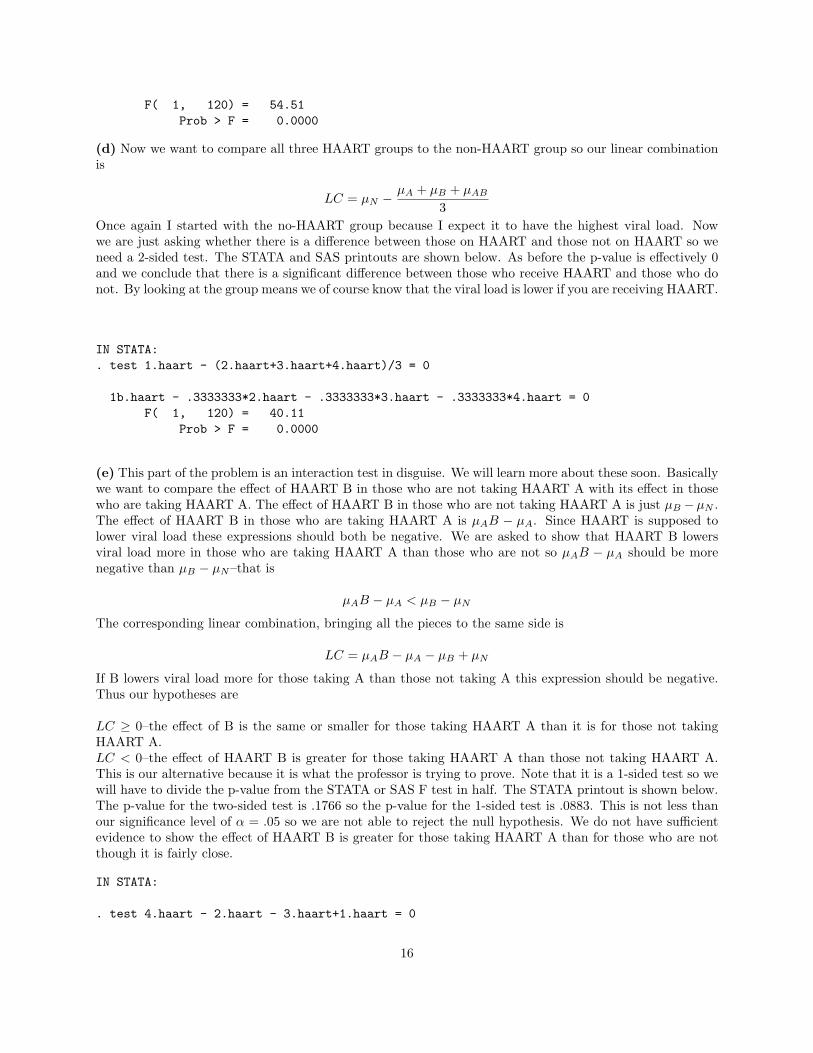
F( 1, 120) = 54.51Prob > F = 0.0000

(d) Now we want to compare all three HAART groups to the non-HAART group so our linear combinationis

LC = µN − µA + µB + µAB

3Once again I started with the no-HAART group because I expect it to have the highest viral load. Nowwe are just asking whether there is a difference between those on HAART and those not on HAART so weneed a 2-sided test. The STATA and SAS printouts are shown below. As before the p-value is effectively 0and we conclude that there is a significant difference between those who receive HAART and those who donot. By looking at the group means we of course know that the viral load is lower if you are receiving HAART.

IN STATA:. test 1.haart - (2.haart+3.haart+4.haart)/3 = 0

1b.haart - .3333333*2.haart - .3333333*3.haart - .3333333*4.haart = 0F( 1, 120) = 40.11

Prob > F = 0.0000

(e) This part of the problem is an interaction test in disguise. We will learn more about these soon. Basicallywe want to compare the effect of HAART B in those who are not taking HAART A with its effect in thosewho are taking HAART A. The effect of HAART B in those who are not taking HAART A is just µB −µN .The effect of HAART B in those who are taking HAART A is µAB − µA. Since HAART is supposed tolower viral load these expressions should both be negative. We are asked to show that HAART B lowersviral load more in those who are taking HAART A than those who are not so µAB − µA should be morenegative than µB − µN–that is

µAB − µA < µB − µN

The corresponding linear combination, bringing all the pieces to the same side is

LC = µAB − µA − µB + µN

If B lowers viral load more for those taking A than those not taking A this expression should be negative.Thus our hypotheses are

LC ≥ 0–the effect of B is the same or smaller for those taking HAART A than it is for those not takingHAART A.LC < 0–the effect of HAART B is greater for those taking HAART A than those not taking HAART A.This is our alternative because it is what the professor is trying to prove. Note that it is a 1-sided test so wewill have to divide the p-value from the STATA or SAS F test in half. The STATA printout is shown below.The p-value for the two-sided test is .1766 so the p-value for the 1-sided test is .0883. This is not less thanour significance level of α = .05 so we are not able to reject the null hypothesis. We do not have sufficientevidence to show the effect of HAART B is greater for those taking HAART A than for those who are notthough it is fairly close.

IN STATA:

. test 4.haart - 2.haart - 3.haart+1.haart = 0

16

( 1) 1b.haart - 2.haart - 3.haart + 4.haart = 0

F( 1, 120) = 1.85Prob > F = 0.1766

IN SAS: (all tests of contrasts for the problem)

proc glm data = work.hw2;class haart;model vload = haart;contrast "1 vs 2" haart 1 -1 0 0;contrast "1 vs 3" haart 1 0 -1 0;contrast "1 vs 4" haart 1 0 0 -1;contrast "2 vs 3" haart 0 1 -1 0;contrast "2 vs 4" haart 0 1 0 -1;contrast "3 vs 2" haart 0 0 1 -1;contrast "1 and 3 vs 2 and 4" haart .5 -.5 .5 -.5;contrast "1 vs 2 vs 3 and 4" haart .5 .5 -.5 -.5;contrast "1 vs 2,3, and 4" haart 1 -.33 -.33 -.33;contrast "interaction" haart 1 -1 -1 1;run; The GLM Procedure

Dependent Variable: vload vload


Model 3 32.23067451 10.74355817 26.94 <.0001

Error 120 47.85296044 0.39877467


R-Square Coeff Var Root MSE vload Mean

0.402463 15.81205 0.631486 3.993702


haart 3 32.23067451 10.74355817 26.94 <.0001


haart 3 32.23067451 10.74355817 26.94 <.0001


17

1 vs 2 1 2.56483007 2.56483007 6.43 0.01251 vs 3 1 7.23556899 7.23556899 18.14 <.00011 vs 4 1 30.30921388 30.30921388 76.01 <.00012 vs 3 1 1.18459848 1.18459848 2.97 0.08742 vs 4 1 15.24021474 15.24021474 38.22 <.00013 vs 2 1 7.92692285 7.92692285 19.88 <.00011 and 3 vs 2 and 4 1 9.75489077 9.75489077 24.46 <.00011 vs 2 vs 3 and 4 1 21.73892159 21.73892159 54.51 <.0001interaction 1 0.73686214 0.73686214 1.85 0.1766

Problems To Turn In

(5) On the Statistical Treadmill:

(a) There are two choices for calculating the confidence intervals for this part of the problem. You caneither calculate a separate standard deviation for each group as if we have three separate samples or youcan use the pooled estimate of the standard deviation from the ANOVA (root MSW). The latter is actuallythe better choice as if the groups all have the same standard deviation (one of the assumptions of a classicalANOVA) then we get the most accurate estimate by using all 18 points and what is more we get to use at-statistic with n−k = 18−3 = 15 degrees of freedom instead of one with 6−1 = 5 degrees of freedom as wewould with individual samples of size 6. The t-value with 15 degrees of freedom will be much smaller, givingus narrower (more precise) confidence intervals. The first set of intervals can be obtained, for example, inSTATA by using the ci command with the bysort option or in SAS using proc univariate with the by option.You can get the intervals using the pooled estimate of the standard deviation from the ANOVA (

√(MSW ).

We accepted either answer as long as you made it clear what you were doing. Below I present both setsof intervals. A plot based on the first set of intervals is shown in the accompanying graphics file. All ofthese intervals overlap, suggesting we can’t be sure any of the means are different although the third group(brochure only) is much lower and barely overlaps the other two groups. As we will see in part (d) theseintervals are very conservative and in fact the difference of this third group turns out to be significant.

Separate Summary Statistics and Intervals Based on The Individual Groups:

IN STATA:. bysort exercisegroup: summarize efficacy

-----------------------------------------------------------------------------------> exercisegroup = 1

Variable | Obs Mean Std. Dev. Min Max-------------+--------------------------------------------------------

efficacy | 6 138.1667 26.35463 100 170

-----------------------------------------------------------------------------------> exercisegroup = 2


18

efficacy | 6 134.6667 17.75012 105 159

---------------------------------------------------------------------------------> exercisegroup = 3


efficacy | 6 108 10.33441 94 124--------------------------------------------------------------------------------

bysort exercisegroup: ci efficacy

-> exercisegroup = 1

Variable | Obs Mean Std. Err. [95% Conf. Interval]-------------+---------------------------------------------------------------

efficacy | 6 138.1667 10.75923 110.5092 165.8242

---------------------------------------------------------------------------------> exercisegroup = 2


efficacy | 6 134.6667 7.246455 116.0391 153.2943

---------------------------------------------------------------------------------> exercisegroup = 3


efficacy | 6 108 4.219005 97.1547 118.8453

-------------------------------------------------------------------------------

IN SAS:proc univariate data = work.hw2;class exercisegroup ;var efficacy;by exercisegroup notsorted; # Note: notsorted was used because the groups wererun; considered not to be in ascending order

The UNIVARIATE ProcedureVariable: efficacy (efficacy)exercisegroup = 1

Moments

N 6 Sum Weights 6Mean 138.166667 Sum Observations 829

19

Std Deviation 26.3546327 Variance 694.566667Skewness -0.3488127 Kurtosis -1.2407518Uncorrected SS 118013 Corrected SS 3472.83333Coeff Variation 19.0745231 Std Error Mean 10.7592338

Basic Statistical Measures

Location Variability

Mean 138.1667 Std Deviation 26.35463Median 142.0000 Variance 694.56667Mode . Range 70.00000

Interquartile Range 37.00000


Moments

N 6 Sum Weights 6Mean 134.666667 Sum Observations 808Std Deviation 17.7501174 Variance 315.066667Skewness -0.5860261 Kurtosis 1.73874358Uncorrected SS 110386 Corrected SS 1575.33333Coeff Variation 13.1807802 Std Error Mean 7.24645507



Mean 134.6667 Std Deviation 17.75012Median 134.0000 Variance 315.06667Mode 132.0000 Range 54.00000



Moments

N 6 Sum Weights 6Mean 108 Sum Observations 648Std Deviation 10.3344085 Variance 106.8Skewness 0.30823179 Kurtosis 0.3171948Uncorrected SS 70518 Corrected SS 534

20

Coeff Variation 9.5688968 Std Error Mean 4.21900462



Mean 108.0000 Std Deviation 10.33441Median 108.0000 Variance 106.80000Mode . Range 30.00000


To get the intervals based on the ANOVA we use the formula

Yj ± tα/2,n−k

√MSW

nj

The linear combination of interest here is simply LC = µj with cj = 1. The sample mean for the groupis our best estimate of the linear combination. The standard error is based on the formula SD(LC) =√

MSW∑

c2j/nj which reduces to

√MSW/nj since the linear combination only has one term. We have

n = 18 data points and 3 groups so we need t.025,15 = 2.13. Since all the groups are the same size theywill all have the same standard error. From the ANOVA printout below we have MSW = 372.14 so thecorresponding standard error is sqrt372.14/6 = 7.88. The resulting intervals are

Group 1: 138.17± (2.13)(7.88) or [121.39, 154.95].Group 2: 134.67± (2.13)(7.88) or [117.89, 151.45].Group 3: 108.0± (2.13)(7.88) or [91.22, 124.78].

Note that the first and second of these intervals are narrower than what we got individually as expected.However the third is actually a bit wider because the standard deviation in the third group seems to be afair bit smaller than in the other two groups, making its individual CI narrower.

(b) We are asked to get the ANOVA table by hand. All we need are the group means and standarddeviations. In this case since the groups are of equal size we can get the overall mean by averaging the threegroup means or of course we could use the summarize or proc univariate commands without the groupingsubcommand. We have Y = 126.9. Using this plus the statistics from above we have

SSB =k∑

j=1

nj(Yj − Y )2 = 6[(138.17− 126.94)2 + (134.67− 126.94)2 + (108− 126.94)2] = 3267

SSW =k∑

j=1

(nj − 1)s2j = 5 ∗ [26.352 + 17.752 + 10.332] = 5580

To get the mean squares you have to divide by the degrees of freedom which are k− 1 for SSB and n− k forSSW. Here we have k = 3 groups and n = 18 total points so

MSB =SSB

k − 1=

3274.442

= 1633.5

21

MSW =SSW

n− k=

5580.4715

= 372

Finally, the F statistic is the ratio of the mean squares which is

F =MSB

MSW=

1633.5372

= 4.39

The resulting ANOVA table is

Source df SS MS FBetween (Treatment) 2 3267 1633.5 4.39

Within (Error) 15 5580 372Total 17 8847

(c) To see whether there is overall evidence of a difference in means we use the ANOVA F test. Our hy-potheses are

H0 : µ1 = µ2 = µ3–there is no difference in average self-efficacy among subjects using the three exerciseregimens.HA : Not all of the µi are equal. There is a difference in average self efficacy between at least two of theexercise regimens.

We can verify the ANOVA table from part (b) in STATA and SAS using the oneway and proc anova com-mands. There are slight differences due to rounding:

IN STATA:. oneway efficacy exercisegroup, tabulate

exercisegro | Summary of efficacyup | Mean Std. Dev. Freq.

------------+------------------------------------1 | 138.16667 26.354633 62 | 134.66667 17.750117 63 | 108 10.334409 6

------------+------------------------------------Total | 126.94444 22.815042 18


------------------------------------------------------------------------Between groups 3266.77778 2 1633.38889 4.39 0.0316Within groups 5582.16667 15 372.144444------------------------------------------------------------------------

Total 8848.94444 17 520.526144

Bartlett’s test for equal variances: chi2(2) = 3.6313 Prob>chi2 = 0.163

IN SAS:

The ANOVA Procedure

Dependent Variable: efficacy efficacy

22


Model 2 3266.777778 1633.388889 4.39 0.0316

Error 15 5582.166667 372.144444


R-Square Coeff Var Root MSE efficacy Mean

0.369171 15.19645 19.29105 126.9444


exercisegroup 2 3266.777778 1633.388889 4.39 0.0316

The p-value for the F test in the ANOVA tables is .0316 which is less than our usual significance level ofα = .05 so we reject the null hypothesis and conclude that there is some difference in self-efficacy amongpeople who used the different exercise regimens. It seems our rough intervals in part (a) did not completelycapture this effect although you will note that the p-value for the F test was actually fairly close to the .05cut off.

(d) The formula for a confidence interval for any linear combination in an ANOVA is

LC ± tα/2,n−k

√MSW

∑c2j/nj

When we are talking about a pairwise difference in means the linear combination is LC = µ1 − µ2 and theconstants are 1 and -1 respectively. Our formula thus becomes

Y1 − Y2 ± tα/2,n−k

√MSW (1/n1 + 1/n2)

If we compare Group 1 and Group 2 in this problem (the ones that got the active exercise interventions)we have Y1 = 138.17, Y2 = 134.67,MSW = 372.14, n1 = n2 = 6. For a 95% confidence interval we needt.025,15 = 2.13. The resulting confidence interval is

138.17− 134.67± (2.13)sqrt372.14(16

+16) = [−20.2, 27.2]

This implies that the self efficacy of people in Group 1 (the full exercise regimen) is anwhere from 20 pointslower to 27 points higher than that of the people in Group 2 (the intermediate exercise regimen). The easiestway to get these intervals on the computer is with the STATA lincom command. The printouts are shownbelow. They confirm the calculation above. The interval comparing Group 1 and Group 2 includes 0 so wecan not be 95% sure these two exercise regimens are different in terms of self efficacy. However, the intervalscomparing each of Group 1 and Group 2 to Group 3 lie entirely above 0, implying that we can be 95% theself efficacy of Group 3 is different (specifically lower) than the other two groups.

. lincom 1.exercisegroup - 2.exercisegroup

23

( 1) 1b.exercisegroup - 2.exercisegroup = 0

------------------------------------------------------------------------------efficacy | Coef. Std. Err. t P>|t| [95% Conf. Interval]

-------------+----------------------------------------------------------------(1) | 3.5 11.13769 0.31 0.758 -20.23943 27.23943

------------------------------------------------------------------------------


( 1) 1b.exercisegroup - 3.exercisegroup = 0


-------------+----------------------------------------------------------------(1) | 30.16667 11.13769 2.71 0.016 6.427241 53.90609

------------------------------------------------------------------------------


( 1) 2.exercisegroup - 3.exercisegroup = 0


-------------+----------------------------------------------------------------(1) | 26.66667 11.13769 2.39 0.030 2.927241 50.40609

------------------------------------------------------------------------------

(e) The intervals in part (a) are for each of the groups individually. There is no correspondence betweenany point in the interval for Group 1 and a specific point in the interval for Group 2. It doesn’t make sensejust to subtract the ends because the intervals are shifted over by the same amount at the high and low ends(approximately so if you use the individual intervals and exactly so if you use the ANOVA based intervals)so we will get a constant difference. About the only thing you can do with the individual intervals is to seeif they overlap–i.e. to compare the high end of one interval to the low end of the other. But this is VERYconservative because the points at the ends of the intervals are the least likely values for the group means(the best estimate is the value in the middle). It is extremely unlikely-much less than .05–that the true meanfor one group will be at the high end of it’s interval at the same time the true mean for the other groupwill be at the low end of it’s interval. What we really need is to know how likely a given COMBINATIONof two mean values is. This can only be done by looking directly at the variability of the DIFFERENCE aswe did in part (d). When we did this the results were much stronger. Another way of saying this is that ifwe do separate intervals for the means we have 2 statements, each of which we are only 95% sure about sowe can not be 95% sure about the overall result whereas if we look at the difference directly we have oneinterval about which we are 95% sure. Looking directly at the interval for the difference is more appropriatesince it correctly accounts for how likely conmbinations of the two group means are. You could also notethat doing individual intervals based on the samples of 6 points would give you smaller degrees of freedomand therefore wider intervals than if you used the pooled estimate of the standard deviation. This is truebut even if we used the pooled estimate of the standard deviation in the individual confidence intervals itwould still not be as good as directly calculating the interval for the difference and indeed when I did thatabove those intervals all overlapped.

(f) Now we want to show that the average efficacy of people doing active exercise is higher than the efficacyof people who only got the brochure. The linear combination of interest is therefore

24

LC =µ1 + µ2

2− µ3

and we are specifically interested in whether this linear combination is greater than 0. Our best estimate ofthe linear combination is

.5 ∗ (Y1 + Y2)− Y3 = .5 ∗ (138.17 + 134.67)− 108 = 28.42

That is, our best guess is that those doing active efficacy have self-efficacy scores on average about 28 pointshigher than those not doing active exercise. As in part (d) we use t.025,15 = 2.13 and the constants for ourlinear combination are c1 = c2 = .5, c3 = −1. The resulting confidence interval is

28.42± (2.13)(

√372.14(

.52

6+

.52

6+

(−1)2

6)) = [7.86, 48.98]

This interval lies entirely above 0 confirming that those who are doing active exercise have higher efficacyscores. If we want to do this as a formal test, our hypotheses are

H0 : .5(µ1 + µ2) − µ3 ≤ 0–the efficacy scores of the active exercisers are the same or lower than the non-exercisers.HA : .5(µ1 + µ2) − µ3 > 0–the efficacy scores of people doing active exercise are higher than those of non-exercisers. This is our alternative hypothesis because it is what we are trying to prove.

The corresponding test statistic is

tobs =LC − 0√

MSW∑

c2j/nj

=28.42− 0

9.65= 2.95

and the corresponding 1-sided p-value is P (t15 ≥ 2.95) = .005. Since this is less than α = .05 we rejectthe null hypothesis and conclude that active exercisers do have higher efficacy scores. The correspondingSTATA and SAS printouts are shown below. They confirm the confidence interval and test statistic. Thep-value given is 2-sided and has to be divide by 2 since we are doing a 1-sided test.

IN STATA:. lincom .5*(1.exercisegroup + 2.exercisegroup) - 3.exercisegroup

( 1) .5 exercisegroup[1] + .5 exercisegroup[2] - exercisegroup[3] = 0


-------------+----------------------------------------------------------------(1) | 28.41667 9.645523 2.95 0.010 7.857721 48.97561

------------------------------------------------------------------------------

IN SAS:proc glm data = work.hw2;class exercisegroup;model efficacy = exercisegroup;contrast "1 and 2 vs 3" exercisegroup .5 .5 -1;run;

Dependent Variable: efficacy efficacy

25


Model 2 3266.777778 1633.388889 4.39 0.0316

Error 15 5582.166667 372.144444


R-Square Coeff Var Root MSE efficacy Mean

0.369171 15.19645 19.29105 126.9444


exercisegroup 2 3266.777778 1633.388889 4.39 0.0316


exercisegroup 2 3266.777778 1633.388889 4.39 0.0316


1 and 2 vs 3 1 3230.027778 3230.027778 8.68 0.0100

(g) If the groups had not been randomly assigned but people had been alllowed to pick their own exerciseregimens it would have been very hard to attribute differences in self-efficacy to the exercise regimens. Itmight well have been the case that people who were more self-confident and already putting more effort intotheir health and personal appearance would have both had higher self-efficacy scores and been more likelyto pick the rigosous exercise programs.

(6) Location, Location, Location:

The primary ANOVA output for this problem is as follows:

\begin{verbatim}. oneway particle location, tabulate

| Summary of particlelocation | Mean Std. Dev. Freq.

---------------+------------------------------------A (class, AC) | 14.2 7.1 25C (cafeteria) | 19.1 6.9 25P (parking lot)| 37.9 6.7 25

26

W (window open)| 36.8 5.1 25R (play yard) | 41.4 8.8 25----------------+------------------------------------

Total | 29.9 13.1 125Analysis of Variance

Source SS df MS F Prob > F------------------------------------------------------------------------Between groups 15181.0047 4 3795.25117 76.70 0.0000Within groups 5937.52594 120 49.4793828------------------------------------------------------------------------

Total 21118.5306 124 170.310731

(a) Here we are being asked to perform an overall F test. Our hypotheses, using the notation of classicalANOVA, are

H0 : µA = µC = µP = µW = µY –the mean pollution level is the same in all 5 of the locations (parking lot,yard, cafeteria, window open classroom, window closed classroom.)HA : Not all the µj ’s are equal. The pollution level is related to which location you are at.

From the printout, the test statistic is a whopping F = 76.7 and the corresponding p-value is 0 to as manydecimal places as STATA gives. We therefore reject the null hypothesis at α = .05 (or any other significancelevel down to .0001) and conclude that pollution level does vary by location on the school grounds. By“real-world” I mean that I want the conclusion in the context of the problem (pollution and location) ratherthan just saying “we reject.”

(b) We skipped this part since we hadn’t fully covered multiple testing by the end of last week. It will beon next week’s homework.(c) To calculate the p-values for the pairwise comparison without using the sort of table generated by theBonferroni command you have to do the contrasts which is a bit slow in STATA as there are 10 of them.In the HW3 solutions I’ll show the trick for doing it faster if you have the table of Bonferroni values. InSAS it’s a little quicker. The printouts are shown below. Note that on the STATA printout location 1is the air-conditioned classroom, location 2 is the cafeteria, location 3 is the parking lot, location 4 is thewindow-open classroom and location 5 is the yard. What we see from these tests is that all the locationcomparisons are significant different at α = .05 except the playground vs the open-window classroom (p =.5745) and the playground and the yard (p = .0769) though this last one is close.

STATA:. test 1.location = 2.location

( 1) 1.location - 2.location = 0

F( 1, 120) = 6.02Prob > F = 0.0156

. test 1.location = 3.location

( 1) 1.location - 3.location = 0F( 1, 120) = 141.66

Prob > F = 0.0000


27


F( 1, 120) = 128.58Prob > F = 0.0000



F( 1, 120) = 187.32Prob > F = 0.0000



F( 1, 120) = 89.29Prob > F = 0.0000



F( 1, 120) = 78.97Prob > F = 0.0000



F( 1, 120) = 126.20Prob > F = 0.0000



F( 1, 120) = 0.32Prob > F = 0.5745



F( 1, 120) = 3.18Prob > F = 0.0769



28

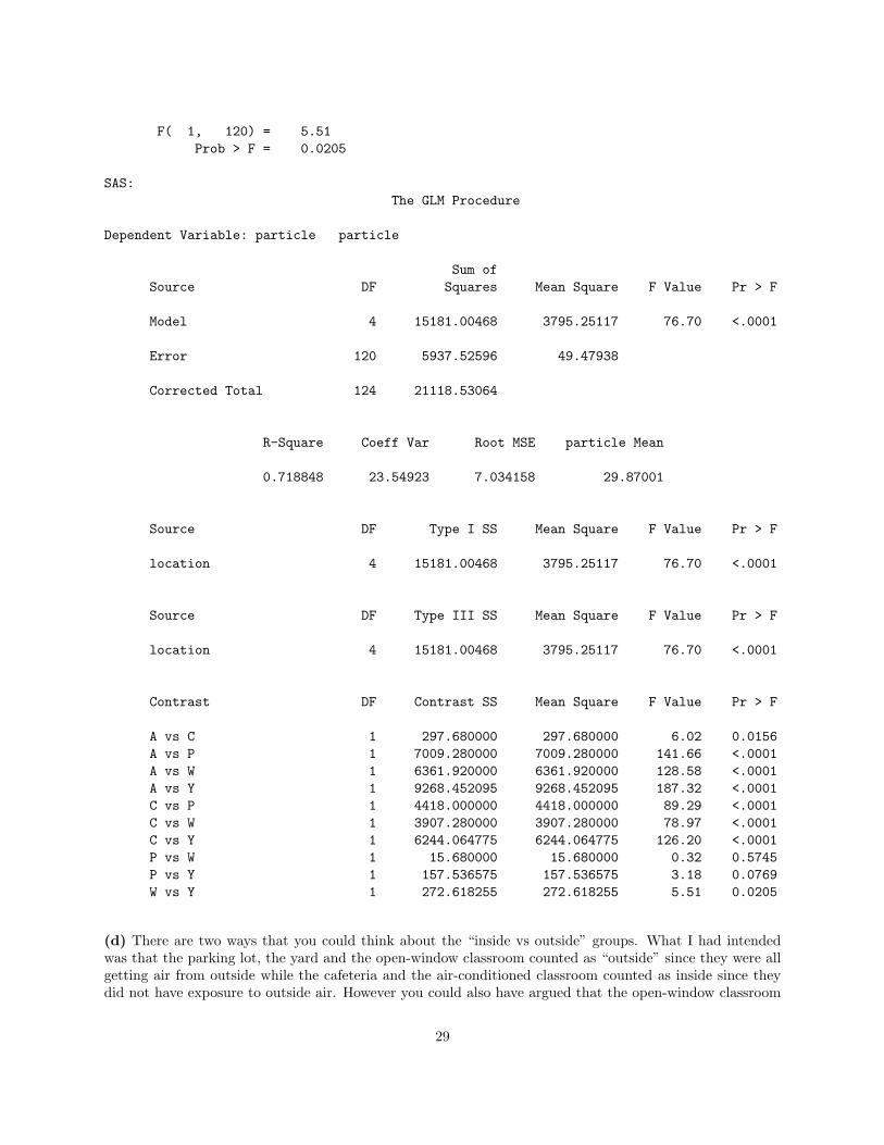
F( 1, 120) = 5.51Prob > F = 0.0205

SAS:The GLM Procedure

Dependent Variable: particle particle


Model 4 15181.00468 3795.25117 76.70 <.0001

Error 120 5937.52596 49.47938


R-Square Coeff Var Root MSE particle Mean

0.718848 23.54923 7.034158 29.87001


location 4 15181.00468 3795.25117 76.70 <.0001


location 4 15181.00468 3795.25117 76.70 <.0001


A vs C 1 297.680000 297.680000 6.02 0.0156A vs P 1 7009.280000 7009.280000 141.66 <.0001A vs W 1 6361.920000 6361.920000 128.58 <.0001A vs Y 1 9268.452095 9268.452095 187.32 <.0001C vs P 1 4418.000000 4418.000000 89.29 <.0001C vs W 1 3907.280000 3907.280000 78.97 <.0001C vs Y 1 6244.064775 6244.064775 126.20 <.0001P vs W 1 15.680000 15.680000 0.32 0.5745P vs Y 1 157.536575 157.536575 3.18 0.0769W vs Y 1 272.618255 272.618255 5.51 0.0205

(d) There are two ways that you could think about the “inside vs outside” groups. What I had intendedwas that the parking lot, the yard and the open-window classroom counted as “outside” since they were allgetting air from outside while the cafeteria and the air-conditioned classroom counted as inside since theydid not have exposure to outside air. However you could also have argued that the open-window classroom

29

was an indoor space. I present both for reference.

(i) Version 1: We wish to compare the mean of the three indoor locations (A, C, W) to the mean of the twooutdoor locations (P,Y). The linear combination corresponding to this comparison is

LC =µA + µC + µW

3− µP + µY

2Note that the linear combination is just the expression for the difference between the groups. It does notinclude the “=0” piece. That is a particular value of the difference that we might be interested in checkingbut it is not formally part of the linear combination itself.

Version 2: Thinking of the open-window classroom as outside we would have (A,C) vs (P,W,Y) or

LC =µA + µC

2− µP + µW + µY

3(ii) To estimate the linear combination we substitute the sample group means for the population groupmeans in the expression above:

LC =YA + YC + YW

3− YP + YY

2=

14.2 + 19.1 + 36.83

− 37.9 + 41.52

= −16.333

Note that you could also reverse the order (taking the outdoor average minus the indoor average) whichwould result in LC = 16.33. All it does is change the sign. If you group the window-open classroom with theplay yard and the parking lot the indoor measurements were 22.083 lower than the outdoor measurements.)

The estimated standard error of a linear combination is given by

s.e.(LC) =

√√√√MSW ∗k∑

j=1

c2j

nj

From the ANOVA table we have MSW = 50, there are nj = 25 measurements at each location, and theconstants in the linear combination are 1/3, 1/3, 1/3,−1/2,−1/2 as I have written it. The correspndingstandard error is

s.e. =

√50(

125

)(3 ∗ (13)2 + 2 ∗ (

−12

)2) =

√2 ∗ (

13

+12) = 1.29

Note that the standard error is the same no matter how you group the inside vs outside locations since eitherway you have 3 of one type and 2 of the other.

(iii) Dr. Green wants to test the hypothesis that air quality inside the classrooms is 10,000cm3 better, i.e.lower inside the buildings than outside. Since my linear combination was set up to subtract the outdoorlocations from the indoor locations and particle concentrations are in thousands, this means I want to provethat my linear combination is less than -10, so that is my alternative hypothesis :

H0 : LC ≥ −10–the pollution levels at the inside locations are not at least 10,000 particles/cm3 better thanin the outdoor locations.HA : LC < −10–the pollution levels for the indoor locations are at least 10,000 particles/cm3 lower than forthe outdoor locations.

The test statistic is

tobs =LC − LCH0

s.e.(LC)=−16.33− (−10)

1.29= −4.91

30

Since we are doing a 1-sided test with an alternative of “less than,” and we have n − k = 120 degrees offreedom associated with our within group variability, our p-value is

p− value = P (t120 ≤ −4.91) = .00000145

I got the exact p-value from STATA using the ttail command. The best you can do from an ordinary t-tableis that t120,.005 = 2.617. Since our test statistic is bigger than this in absolute value, the p-value must be lessthan .005. In any case, we clearly reject the null hypothesis at α = .05 and conclude that the pollution levelis at least 10,000 particles/cm3 better inside than outside. You get this conclusion even more strongly if yougroup the open window classroom with the outdoor measurements since its mean was more like the otheroutdoor locations than the other indoor locations. Of course you could use the test procedure in STATAafter the anova command or another contrast statement in SAS to do this problem instead of the handcalculations! These outputs are shown below. Note that you need to be careful to get the groups in theright order! The classroom with the window open is the 4th category.....Also, SAS really likes it’s contrastcoefficients to add up exactly to 0 so I used .33, .33 and .34 as the coefficients in the contrast statement.

STATA:test (1/3)*(1.location+ 2.location + 4.location) - .5*(3.ocation + 5.location) = 0

( 1) .3333333 1.location + .3333333 2.location + .3333333 4.location -.5 3.location - .5 5.location = 0

F( 1, 120) = 161.26Prob > F = 0.0000

test .5*(1.location+ 2.location) - (1/3)*(3.location + 5.location) = 0

( 1) .5 1.location + .5 2.location + -.333333 3.location - .3333334.location - .33333 5.location= 0

F( 1, 120) = 294.79Prob > F = 0.0000

SAS:

proc glm data = tmp3.hw2;class location;model particle = location;contrast "A,C, W vs P, Y" .33 .33 -.5 .34 -.5;contrast "A, C vs P, W, Y" location .5 .5 -.33 -.33 -.34;run;

The GLM Procedure

Dependent Variable: particle particle


Model 4 15181.00468 3795.25117 76.70 <.0001

31

Error 120 5937.52596 49.47938


R-Square Coeff Var Root MSE particle Mean

0.718848 23.54923 7.034158 29.87001


location 4 15181.00468 3795.25117 76.70 <.0001


location 4 15181.00468 3795.25117 76.70 <.0001


ACW vs PY 1 7847.54368 7847.54368 158.60 <.0001AC vs PWY 1 14621.20505 14621.20505 295.50 <.0001

32

solutions to homework assignment 2 warm-up...

Documents