solutions of flexible polymers. neutron experiments and ... · occur; fortunately the theory of...

804 Jannink et al. Macromolecules

(21) S. Saeki, N. Kuwahara, S. Konno, and M. Kaneko, Macromolecules, 6,

(22) N. Kuwahara, S. Saeki, T. Chiba, and M. Kaneko, Polymer, 15, 777

(23) S. Saeki, S. Konno, N. Kuwahara, M. Nakata, and M. Kaneko, Macro-

(24) L. P. McMaster, Macromolecules, 6,760 (1973). (25) M. Bank, J. Leffingwell, and C. Thies, J . Polym. Sci., Par t A-2, 10,

(26) P. J. Flory and H. Hocker, Trans. Faraday Soc., 2258 (1971). (27) H. Hocker, H. Shih, and P . J . Flory, Trans. Faraday Soc., 2275 (1971). (28) P. J. Flory and H. Shih,Macromolecules, 5,761 (1972). (29) P . Ehrlich and J. J. Kurpen, J . Polym. Sci., Par t A, 1,3217 (1963). (30) C. D. Myrat and J. S. Rowlinson, Polymer, 6,645 (1965). (31) S. Saeki, N. Kuwahara, M. Nakata, and M. Kaneko, Polymer, 16, 445

(32) K. Sugamiya, N. Kuwahara, and M. Kaneko, Macromolecules, 7, 66

(33) R. Koningsveld, H. A. G. Chermin, and M. Gordon, Proc. R. Soc. Lon-

246,589 (1973).

(1974).

molecules, 7,521 (1974).

1097 (1972).

(1975).

(1974).

don, Ser. A, 319,331 (1970).

(34) N. Kuwahara, M. Nakata, and M. Kaneko, Polymer. 14,415 (1973). (35) The data of the ucst and lcst for the solution of polystyrene in tert-

butyl acetate, ethyl formate, methyl acetate, ethyl n-butyrate, diethyl malonate, and sec-butyl acetate and of the ucst for the polystyrene- trans-decalin will be supplied on request. For the polystyrene-trans- decalin system no phase separation was observed up to the highest temperature (360’C) we could readily attain.

(36) S. Saeki, N. Kuwahara, and M. Kaneko, to be published. (37) C. Reiss and H. Benoit, J . Polym. Sci., Par t C, 16,3079 (1965). (38) P. J. Flory, “Principles of Polymer Chemistry”, Cornell University

(39) N. Kuwahara, S. Saeki, S. Konno, and M. Kaneko, Polymer, 15, 66

(40) H. Tompa, “Polymer Solutions”, Butterworths, London, 1956. (41) B. E. Echinger, J . Chem. Phys., 53,561 (1970). (42) T . A. Orofino and A. Ciferri, J . Phys. Chem., 68,3136 (1964). (43) P . J. Flory, “Statistical Mechanics of Chain Molecules”, Wiley, New

(44) H. Hocker, G. J. Blake, and P. J. Flory, Trans. Faraday Soc., 67,2251

Press, Ithaca, N.Y., 1953.

(1974).

York, N.Y., 1969, p 45.

(1971).

Solutions of Flexible Polymers. Neutron Experiments and Interpretation

M. Daoud,la J. P. Cotton,’a B. Farnoux,la G . Jannink,*la G . Sarma,la H. Benoit,lb R. Duplessix,lb C. Picot,lb and P. G . de Gennedc Laboratoire Lkon Brillouin, Centre d’Etudes Nuclkaires de Saclay, 91190 Gif-sur-Yvette, France; Centre de Recherches sur les Macromolkcules, 67083 Strasbourg Cedex, France; and College de France, 1 1 , Place M . Berthelot, 75005 Paris, France. Received May 13, 1975

ABSTRACT: We present small angle neutron scattering data on polystyrene (normal or deuterated) in a good solvent (carbon disulfide). All data are taken in the semidilute regime where the chains overlap strongly, but the solvent fraction is still large. We have measured the following. (a) The radius of gyration RG(c) for one deuterated chain in a solution of normal chains with concentration c . We find that R G ~ ( c ) is proportional to the molecular weight and that R G ~ decreases with concentration like c - ~ where x = 0.25 f 0.02. (b) The screening length { ( c ) (introduced, but not quite correctly calculated by Edwards) giving the range of the ( c ( r ) c ( r ’ ) ) correlations. We find { - c - ~ , with z = 0.72 f 0.06. (c) The osmotic compressibility x ( c ) (through the scattering intensity of identical chains in the small angle limit). From an earlier light-scattering experiment, we find x - c - Y with y = 1.25 f 0.04. These results are to be compared with the predictions of the mean field (FlorylHuggins-Edwards) theory which are: Rc independent of c , x - c - l , and { - c-lI2 in the semidilute range. We show in the present paper that the measured exponents can all be interpreted in terms of a simple physical picture. The underlying basis is the analogy, recently found by Des Cloizeaux, between the semidilute system and a ferromagnet under an external field. However, in this paper, we emphasize mainly the polymer aspects. At short distances ( r < [) the correlations are determined by excluded volume effects. At large distances ({ < r < RG) the chains are gaussian and the effective interaction between subunits of the same chain are weak.

I. Introduction 1. General Aims. For a long time, the main experiments

on polymer solutions measured macroscopic parameters such as the osmotic pressure, or the heat of dilution. The resulting data for good solvents are rather well systematized by a mean field theory analysis due to FloryZa and Huggins.2b A precise description of the method and some of the data can be found in chapter 12 of Flory’s book.3 Re- cently, however, it has become possible to probe solutions more locally (Le., a t distances of order 20 to 500 A) by small-angle neutron ~ca t te r ing .~ Using the large difference between the scattering amplitude of protons and deuter- ons, many different measurements become feasible. For instance it is possible to study one single-labeled chain among other chains which are chemically identical, but not labeled.5 In the present report we present two distinct series of neutron studies on polymer solutions: one with identical chains, and another one with a few labeled chains. These experiments prove that the mean field theory must be refined, and that a number of anomalous exponents

occur; fortunately the theory of polymer solutions in good solvents has progressed remarkably in the last year mainly through the work of Des Cloizeaux.6 In his original article, Des Cloizeaux was concerned mainly with thermodynamic properties. In the theoretical part of the present paper, we show that (a) his results can be derived directly from certain scaling assumptions and (b) his arguments can be ex- tended to discuss local correlation properties. Our discussion is only qualitative, but it does account for the anomalous exponents, without the heavy theoretical background which is needed to read ref 6. (A simplified version of ref 6, requiring only a modest knowledge of magnetism and phase transitions, is given in the Appendix.) To reach a (hopefully) coherent presentation, we shall not separate the theory from the experiments, but rather insert the latter a t the right point in the discussion.

2. Organization. This paper is organized as follows. Sec- tion I1 describes the experimental method. Section I11 contains a general presentation of the three concentration do- mains for polymer solutions, corresponding respectively to

Vol. 8, No. 6, November-December 1975 Neutron Experiments and Interpretation 805

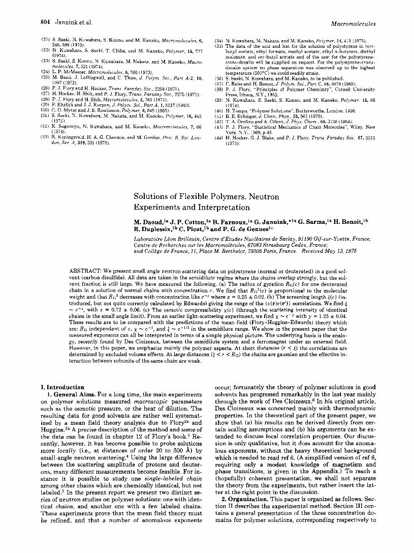
1 Figure 1. Scattered intensities I(r) as a function of the distance r between a cell detector and the direct beam: r is a measure of the scattering angle 8, r/L = 8, where L is the path length between sample and detector. Open circles: scattered intensity by a solution of 0.5 X g cm-3 PSD and 95 X loW2 g cm-3 PSH in CS2. Closed circles: scattered intensity by a solution of 95 X g cm-3 PSH in CS2. The intensity variation a t small r is due to the direct beam contamination.

separated chains, overlapping chains, and concentrated systems. Our interest is mainly on the second, “semidilute” regime. We discuss in section I11 the global thermodynamic properties in this regime. In section IV we consider the local structure of the correlation, and establish the distinc- tion between a short-range behavior which is of the excluded volume type and a long-range behavior which corresponds essentially to gaussian chains; the critical distance F a t which these two pictures merge is one crucial parameter of the theory and we report measurements of this length as a function of concentration. Finally, in section V, we discuss possible correlation experiments involving chains which carry a label a t one definite position (for instance at the ends, or a t the midpoint).

11. Experimental Technique 1. Contrast Factor in a Small-Angle Neutron-Scattering

Experiment. The scattering of a radiation of wavelength X by a medium with long-range correlations (Le., greater than A) gives rise to a central intensity peak about the forward scattering direction. The shape of this peak reflects the pair correlation function of the atoms in the sample. The intensity is determined by the interaction between radiation and atoms. In case of a neutron radiation, the interaction is of the neutron-nucleus type. I t is characterized by a “coherent scattering length”, a . The value of u varies in an impredictable manneri from nucleus to nucleus. For example, the hydrogen atom has a scattering length QH = -0.374 X cm, and the deuterium atom has U D = +0.670 X cm. This is the large difference responsible for the success of the labeling meth- od8.g in the study of polymer configurations by small-angle neutron scattering. The labeling is an isotopic substitution, without chemical perturbation.

In a scattering experiment the intensity is recorded as a function of the scattering angle 8. The pair correlation function S ( q ) , for a given scattering vector

14 = 4 ~ l X sin 8/2 (11.1)

I ( q ) = AK2S(q) (11.2)

is related to the coherent scattered intensity I ( q ) by

where A is the apparatus constant and K the contrast factor or “apparent” scattering amplitude given by

K = ( a , - na,) (11.3)

a, is the coherent scattering length for the monomer unit (i.e., the sum of the length associated with each atom), us is the coherent scattering length for the solvent molecule, and n is the ratio of the

Table I Characteristics of Samples 1 and 2

Sample Poly- c *, no. mer .wW M,JV~ g A

~~

5.62

0.020 8.83

1 PSD 114000 1.10 o.075 PSH 114000 1.02

2 PSD 500000 1.14 PSH 530000 1.10

partial molar volumes. Formula 11.2 can be generalized to the problem of interest in the study of concentrated solutions, where a few labeled chains are dispersed in a solution of unlabeled chains and solvent. In this case

I ( q ) = A[KD2SD(q) -k K H 2 S H ( q ) -k BKDKHSHD(Q)] (11.4)

where the separate correlation functions for labeled and unlabeled polymers are respectively s D ( q ) and SH(4); SHD is the interference term, K D and K H are the “apparent” scattering amplitudes defined by eq 11.3 for the deuterated and protonated monomers, respectively. For polystyrene dissolved in carbon disulfide, the theoretical values’O for these amplitudes are

K D = 8.6 X cm

K H = 0.3 X cm

I t is clear, with these numbers, that the scattered intensity (eq 11.4) is essentially proportional to the correlation function of the labeled chains; this assertion is true a t about every practical concentration of deuterated and protonated chains, as will be seen from the concentration dependence of s D ( q ) and S H ( 4 ) in section IV.

Up to this point we have only discussed the “coherent” contribution to the scattered intensity. The presence of protons in the solution implies however a strong “incoherent” contribution to the scattered intensity, which is q independent. Because of the long- range monomer-monomer correlation, the weight of the coherent signal is of an order of magnitude greater than the incoherent signal. The two contributions can be compared in Figure 1. The upper curve corresponds to a concentration C D = 5 X g cm-3 of labeled chains and a concentration C H = 95 X g cm-3 of protonated chains, dispersed in carbon disulfide. The lower curve corresponds to the solution of protonated chains only ( C H = 95 X lo-” g cm-“). I t is seen to contribute by an order of magnitude less.

2. Samples. Our experiments have been carried out with two kinds of polystyrene chains. (a) The first is deuterated polystyrene (PSD), obtained by anionic polymerization of perdeuterated styrene (kindly supplied by Mr. M. Herbert, CEA, DBpartement des RadioBlBments). The method of preparation and the characteriza- tion are detailed in ref 11. The molecular weights and polydispersity are given in Tables I and I11 (section IV). (b) The second kind of chain is hydrogeneous polystyrene, prepared by anionic polymerization (cf. Table I). The samples are mixtures of PSD and PSH, in proportions described in section IV, dispersed in carbon disulfide. This is a good solvent and has the advantage of being “transparent” to the neutron beam.

3. Apparatus. The wavelength of the incident neutron beam can be fixed in between X = 5 A and 10 A. This range is very convenient for a study of polymer configuration and points out another advantage of neutron-scattering technique. I t allows the measure- ment of the size of the polymer coil in the “Guinier” range, as in a light-scattering experiment,

qRc, < 1 (11.5)

where Rc is the radius of gyration of the coil, and also the monomer-monomer correlation function in the so called “asymptotic” or “intermediate” range

l / R G < q < 1/1 (11.6)

where 1 is the step length. Measurements of Rc, were performed with the small-angle neu-

tron-scattering apparatus a t the “Institut Laue Langevin” (Greno- ble) (the “Institut Laue Langevin” has edited a Neutron Beam Fa- cilities available for users, ILL, BP 156 Centre de tri 38042 Greno- ble). The experimental setup is described in ref 11 and corresponds to the lines B and C of Table I11 of this reference. The incident beam has a broad wavelength distribution and the momen-


tum transfer is defined here as inversely proportional to the mean quadratic wavelength XO

(11.1‘)

The values of XO are given in Table I. For the intermediate momentum range (eq 11.6), the measure-

ments were made on a two-axis spectrometer at the exit of a “cold” neutron guide of the EL3 reactor at Saclay, specially designed for small-angle scattering. A detailed description is also given in ref 11. The incident wavelength is 4.62 f 0.04 (thus with a very narrow distribution as compared to the first apparatus) and the scattering vector range is

q = 4 ~ 1 x 0 sin el2

10-2 A-1 5 q 5 10-1 A-1

111. Different Concentration Regimes and Global Properties

All our discussion will be restricted to the case of good solvents, where different monomers repel each other.

1. Dilute Limit. In this limit, the chains are well separated and behave essentially like a gas of hard spheres,12 with a radius43

RG N Nu (111.1)

Here N is the polymerization index (the number of monomers per chain) and v is an excluded volume exponent. We shall always use the Flory value3 for v ; in the space dimension d = 3, v = 3/6. This value is confirmed by a large number of experiments13 and by numerical studies.14 Recent advances in the theory of phase transitions15 have shown that it is instructive to consider not only the usual case d = 3, but also other possible dimensionalities (d = 2, for instance, corresponds to polymer films on a surface). The general Flory formula for d I 4 is

v = 3/(d + 2) (111.2)

Above four dimensions, v sticks to the ideal chain value (v = YZ).

The dilute regime corresponds to chain concentrations pp = p/N such that the coils are mostly separated from each other

p@Gd = p f l d << 1 (111.3)

In this limit the osmotic pressure A is given by a virial ex- p a n ~ i o n ~ ~

(111.4)

where M is the molecular weight of the polymer chain. The quantity A2 is a second virial coefficient. (The notation A2(0) recalls that it is defined here in the dilute limit.) As in a hard sphere system, Az(0) is proportional to the volume occupied by one chain

A2(0) = aRed/6M2 - N”d-2 (111.5)

Equations 111.1, 111.4, and 111.5 have been amply verified3 and we have nothing to add here. But eq 111.4 and 111.5 will be of use later for comparison with the behavior found at higher concentrations.

2, Semidilute Solutions. This regime sets in when p & ~ d > 1. The chains now interpenetrate each other and the thermodynamic behavior becomes completely different. In terms of the monomer concentration p, the semidilute regime is defined by the two inequalities

p* << p << 1 (111.6)

C = - + A2(0)c2 + , . ,

M

where we have introduced a critical concentration

p* = NRG-d = N1-ud = C*D (111.7)

In our experiments p* ranges between The changes occurring near p = p* have been studied by various methods and in particular by neutron ~ca t te r ing .~ Here we shall be more concerned with the region above p* defined by (111.6).

In this region the mean field picture could be presented as follows: for small p the free energy density is of the form

(111.8)

where Fideal is the free energy for nonintersecting coils with their unstretched radius RGO = N1f2, and V is the volume of the sample. The parameter u (with dimension volume) is a virial coefficient for the monomer-monomer interaction. One definition of u follows the paper by Edwards.I6 In the Flory notation we would write

and 8 X

T d3r V F = Pideal -t ; u Sp2(r) - + O(p3)

where V1 is the molar volume of the solvent and mo the molecular weight of the monomer. The constant x1 charac- terizbs the solvent-solute interaction, $1 is the entropy constant, and 0 is the Flory temperature.

We restrict our attention to good solvents where u is positive. Returning now to eq 111.8 the mean-field approximation amounts to replacing p2(r) by p2. The osmotic pressure is related to F by the general formula

(111.10) a

A = pp2- ( E ) aPP PP

(since l/pp is the volume per chain and F/pp is the free energy per chain). Using pp = PIN, eq 111.10 may also be written as:

.I+(-) a F aP P

(111.10’)

Writing F = Fideal + %Tup2 in the mean-field approximation we get

The first term (derived from Fideal) is in fact negligible for semidilute solutions. Thus the mean-field prediction is essentially

A 1 u T 2m02

C2 _ - - -- (111.11)

We notice that at a given concentration c in this range, the osmotic pressure is independent of the chain molecular weight. (In the dilute range, *IT is strongly dependent upon M (eq III.4).)

However, this formula omits a very important correlation effect; when one monomer is located at point r, all other monomers are repelled from the vicinity of r. Thus the average of p2 ( r ) is expected to be smaller than p2. (Also, as we shall see, the chains are still swollen in the semidilute region; this reacts on the entropy.) To include all these effects, let us assume that the osmotic pressure behaves like some powers of the concentration

(111.12) _ - - constant X cm T

This particular scaling law can be, to some extent, demon- strated by a renormalization group technique17 or related to the scaling properties of a magnetic system.6 If we accept it, we can derive the value of the exponent m by asking that eq 111.4 and 111.12 give the same order of magnitude at the

a


F(c

0.2

0.1

I

0 0.01 0.02 g,cnr3 0.03 0.04

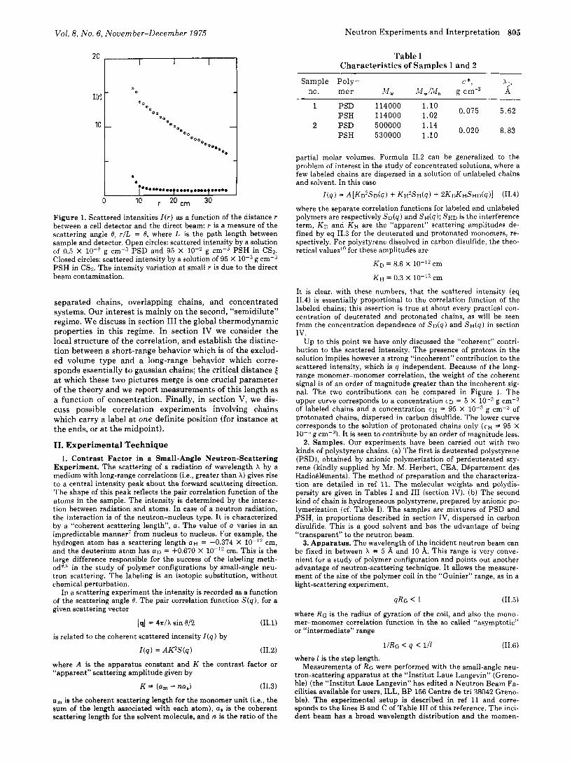
Figure 2. Representations of the osmotic pressure vs. concentrations. The data of ref 18 are divided by c 2 (open circles) and by c9/4 (closed circles). The latter representation illustrates the proposi- tion that in the semidilute range, the osmotic pressure behaves as c9l4 rather than the mean field value c2.

crossover between dilute and semidilute regimes (c = c * )

(111.13) C * N - N constant x ( c * ) ~

Inserting the value from eq 111.7 for c* gives

m = ud/(ud - 1) (111.14)

a value first derived in ref 6. For d = 3, and using v = 3/5 , one finds m = 9/4, to be compared to the mean-field value m = 2. The difference is not very large but, as we shall see it, visible in careful experiments performed with sufficiently long chains (a large N is favorable, because it gives a small c* and thus a wide range of semidilute systems).

(a) There are many data in this field3 of osmotic pressure measurements. We shall discuss here the findings of Stra- zielle and coworkers,ls who measured the pressures a t the highest possible concentrations beyond c* in order to detect deviations from the c2 behavior. Figure 2 shows two representations of these data, respectively *IC2 and T / C ~ / ~ .

The two curves illustrate the discussion about the exponent m. The figure is however not intended as a proof of eq 111.12. The evidence which we consider as an experimental proof for the value of m is given in section IV.

(b) The heat of dilution, MI, and the specific heat of dilution m 1 , can be calculated as a function of c. A definition of AH1 is3

AH1 = t P l 2 (111.15)

where { is the change of energy for the formation of unlike contacts and p12 is the number of such pairs. This quantity is evaluated as follows. The probability that a site is occupied by a (polymer) segment is p. Formula 111.12 tells us that the probability for another segment to be in an adja- cent site is p x p5l4. In other words, the conditional probability for a segment to occupy a site, knowing that an adja- cent site is occupied by another segment, is p5/4. This quantity is smaller than p; there is a depletion effect around each site occupied by a polymer segment. The probability for unlike contacts is thus

1 I I I 1

10-1

2 c 5 10-2

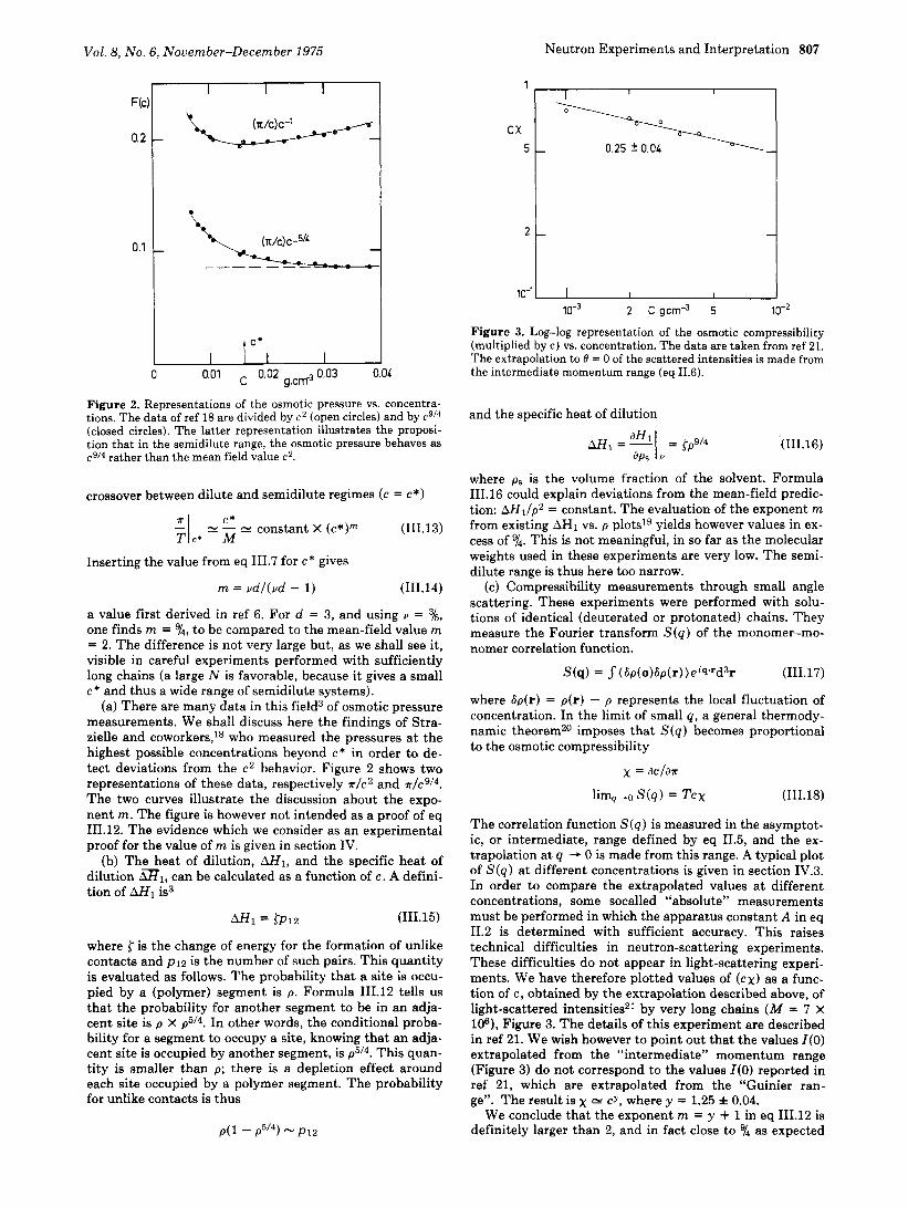
Figure 3. Log-log representation of the osmotic compressibility (multiplied by c ) vs. concentration. The data are taken from ref 21. The extrapolation to 0 = 0 of the scattered intensities is made from the intermediate momentum range (eq 11.6).

and the specific heat of dilution

(111.16)

where ps is the volume fraction of the solvent. Formula 111.16 could explain deviations from the mean-field prediction: AHl/p2 = constant. The evaluation of the exponent m from existing AH1 vs. p plotslg yields however values in ex- cess of 9/4. This is not meaningful, in so far as the molecular weights used in these experiments are very low. The semidilute range is thus here too narrow.

(c) Compressibility measurements through small angle scattering. These experiments were performed with solutions of identical (deuterated or protonated) chains. They measure the Fourier transform S(q ) of the monomer-monomer correlation function.

S(q) = S(bp(o)dp(r))eis.’d3r (111.17)

where 6p(r) = p(r) - p represents the local fluctuation of concentration. In the limit of small q , a general thermodynamic theoremz0 imposes that S(q) becomes proportional to the osmotic compressibility

x = ac/ar

lim,-0 S(q) = Tcx (111.18)

The correlation function S(q) is measured in the asymptotic, or intermediate, range defined by eq 11.5, and the extrapolation a t q - 0 is made from this range. A typical plot of S(q) at different concentrations is given in section IV.3. In order to compare the extrapolated values a t different concentrations, some socalled “absolute” measurements must be performed in which the apparatus constant A in eq 11.2 is determined with sufficient accuracy. This raises technical difficulties in neutron-scattering experiments. These difficulties do not appear in light-scattering experiments. We have therefore plotted values of ( c x ) as a function of c, obtained by the extrapolation described above, of light-scattered intensitiesz1 by very long chains (M = 7 x lo6), Figure 3. The details of this experiment are described in ref 21. We wish however to point out that the values Z(0) extrapolated from the “intermediate” momentum range (Figure 3) do not correspond to the values Z(0) reported in ref 21, which are extrapolated from the “Guinier range”. The result is x = cy, where y = 1.25 f 0.04.

We conclude that the exponent rn = y + 1 in eq 111.12 is definitely larger than 2, and in fact close to y4 as expected


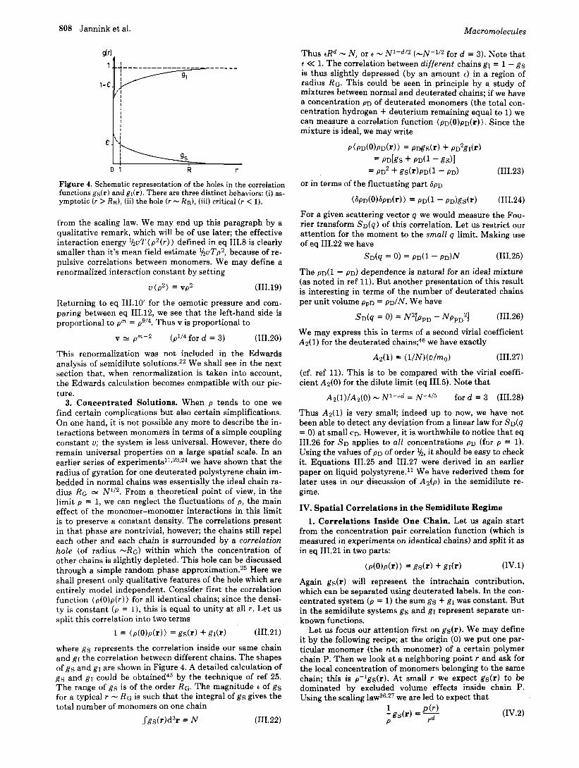
Figure 4. Schematic representation of the holes in the correlation functions gs(r) and gl(r). There are three distinct behaviors: (i) asymptotic ( r > RR), (ii) the hole ( r - RR) , (iii) critical ( r < 1).

from the scaling law. We may end up this paragraph by a qualitative remark, which will be of use later; the effective interaction energy MuT(p2(r) ) defined in eq 111.8 is clearly smaller than it's mean field estimate 'huTp2, because of re- pulsive correlations between monomers. We may define a renormalized interaction constant by setting

v ( p 2 ) = vp2 (111.19)

Returning to eq 111.10' for the osmotic pressure and comparing between eq 111.12, we see that the left-hand side is proportional to pm = p9/4. Thus v is proportional to

v N pm-2 (p1l4 for d = 3) (111.20)

This renormalization was not included in the Edwards analysis of semidilute solutions.22 We shall see in the next section that, when renormalization is taken into account, the Edwards calculation becomes compatible with our picture.

3. Concentrated Solutions. When p tends to one we find certain complications but also certain simplifications. On one hand, it is not possible any more to describe the interactions between monomers in terms of a simple coupling constant u; the system is less universal. However, there do remain universal properties on a large spatial scale. In an earlier series of experiment^"^^^^^^ we have shown that the radius of gyration for one deuterated polystyrene chain im- bedded in normal chains was essentially the ideal chain radius RG = N112. From a theoretical point of view, in the limit p = 1, we can neglect the fluctuations of p, the main effect of the monomer-monomer interactions in this limit is to preserve a constant density. The correlations present in that phase are nontrivial, however; the chains still repel each other and each chain is surrounded by a correlation hole (of radius -RG) within which the concentration of other chains is slightly depleted. This hole can be discussed through a simple random phase a p p r o x i m a t i ~ n . ~ ~ Here we shall present only qualitative features of the hole which are entirely model independent. Consider first the correlation function (p(O)p(r)) for all identical chains; since the density is constant ( p = I ) , this is equal to unity at all r. Let us split this correlation into two terms

(111.2 1)

where gs represents the correlation inside our same chain and g1 the correlation between different chains. The shapes of g s and gl are shown in Figure 4. A detailed calculation of gs and gl could be obtained45 by the technique of ref 25. The range of g s is of the order RG. The magnitude t of gs for a typical r - Rc, is such that the integral of gs gives the total number of monomers on one chain

1 = (p(O)p(r)) = gdr) + gdr)

jgs(r)d"r = N (111.22)

Thus tRd - N , or t - N1-d /2 (-N-lI2 ford = 3). Note that t << 1. The correlation between different chains gI = 1 - gs is thus slightly depressed (by an amount t ) in a region of radius RG. This could be seen in principle by a study of mixtures between normal and deuterated chains; if we have a concentration p~ of deuterated monomers (the total concentration hydrogen + deuterium remaining equal to 1) we can measure a correlation function (PD(O)pD(r)). Since the mixture is ideal, we may write

P(PD(O)PD(r)) = PDgS(r) + PD2gI(r) = P D k S + PD(1 - gS)]

= PD2 + gS(r)PD(1 - PD) (111.23) or in terms of the fluctuating part b p ~

(h'D(o)&PD(r)) = PD(1 - PD)gS(r) (111.24) For a given scattering vector q we would measure the Fou- rier transform s D ( q ) of this correlation. Let us restrict our attention for the moment to the small q limit. Making use of eq 111.22 we have

s D ( q = 0 ) = P D ( 1 - PD)N (111.25)

The pD(1 - p ~ ) dependence is natural for an ideal mixture (as noted in ref 11). But another presentation of this result is interesting in terms of the number of deuterated chains per unit volume p p ~ = ~ D / N . We have

s D ( q = 0) = N2[PpD - NppD2] (111.26)

We may express this in terms of a second virial coefficient A2( 1) for the deuterated chains;46 we have exactly

Ad11 = (l/N)(o/mo) (111.27)

(cf. ref 11). This is to be compared with the virial coefficient Az(0) for the dilute limit (eq 111.5). Note that

A2(l)/A2(0) - N1-ud = N-4/5 ford = 3 (111.28)

Thus Az(1) is very small; indeed up to now, we have not been able to detect any deviation from a linear law for s D ( q = 0) a t small CD. However, it is worthwhile to notice that eq 111.26 for SD applies to all concentrations p~ (for p = 1). Using the values of p~ of order I,&, it should be easy to check it. Equations 111.25 and 111.27 were derived in an earlier paper on liquid polystyrene." We have rederived them for later uses in our discussion of A&) in the semidilute regime.

IV. Spatial Correlations in the Semidilute Regime 1. Correlations Inside One Chain. Let us again start

from the concentration pair correlation function (which is measured in experiments on identical chains) and split i t as in eq 111.21 in two parts:

Again gdr) will represent the intrachain contribution, which can be separated using deuterated labels. In the concentrated system ( p = 1) the sum gs + gI was constant. But in the semidilute systems gs and gI represent separate un- known functions.

Let us focus our attention first on g&). We may define it by the following recipe; a t the origin (0) we put one particular monomer (the nth monomer) of a certain polymer chain P. Then we look a t a neighboring point r and ask for the local concentration of monomers belonging to the same chain; this is p-lgs(r). At small r we expect gs(r) to be dominated by excluded volume effects inside chain P. Using the scaling la^^^*^^ we are led to expect that

(IV.2)


where p ( r ) is the number of chain units which will give a coil of size r . Thus p ( r ) N r1lU and

1 - gs(r) = r-d+l/u E r--4/3 ford = 3 (IV.3) P

Equation IV.3, for an isolated chain, was written down long ago by Edwards.l6 This single chain behavior will apply whenever the local concentration p-’gs(r) due to a chain P is larger than the average concentration p (due to other chains). The cross-over will thus occur a t a certain characteristic distance such that

(IV.4) 1 P - & ( E ) = P

Equation IV.3 then shows that

or

6 = p-3/4 for d = 3 (IV.5)

In a recent e ~ p e r i m e n t , ~ the single chain behavior could be observed at concentrations substantially greater than p*.

At the lower concentration limit (p = p’) the length 5 is equal to the coil size Rc(p*) - NY. At higher concentrations

E is smaller than RG(P). Ultimately, for p equal to unity becomes of order one (i.e., comparable to the monomer size). In this limit all effects of the anomalous exponent u are removed. This is why the simple random phase calculation of ref 25 is acceptable for molten polymers.

At distances larger than E , the chain P may be considered as a succession of statistical elements, with a number of monomers per element p ( & ) - [l/”. The average square length of one element is E2. Successive elements are screened out from each other by the other chains, and the overall behavior is thus expected to be gaussian. Thus the end-to-end distance R(p) is given by

Equation IV.6 can also be derived from the Des Cloiseaux approach (see Appendix).

(a) Radius of Gyration. From relation IV.6, the c and M dependence of R2(c ) is

R2(c ) - Mw~-1/4 for d 3 (IV.7)

where M, is the molecular weight average. In order to test the validity of this relation, we have mea-

sured the radii of gyration of the PSD chain dispersed in a PSH and CS2 solution. Two sets of PSD, PSH, and CS2 solutions have been used, corresponding to the two molecular weights given in Table I.

The data were obtained using the small angle apparatus a t the I.L.L. with the set-up described in section 11. The two values of the quadratic mean wavelength of the incident beam (given in Table I) are chosen to match, for each set of samples, the inequality qRG(c) < 1 (11.1’).

The radius of gyration, R G ( c ) , of a chain dispersed in a solution with chain concentration c is measured from the pair correlation of the labeled chains. Although the concentration CD of labeled chains is small compared to c, there are interference terms which must be evaluated. This is achieved by extrapolation of the data a t CD = 0 while main- taining the total concentration c fixed. For each total concentration c, eight samples are studied; four solutions are made with the concentrations CD = 0.020,0.015,0.010, and 0.005 g of PSD (each containing a concentration CH of PSH such that the sum CH + CD remains equal to c ) . The four others are test samples which contain only the four

11 I I I I I

I

I I I I 0 0.5 1.0 1.5 2.0

CD +a+

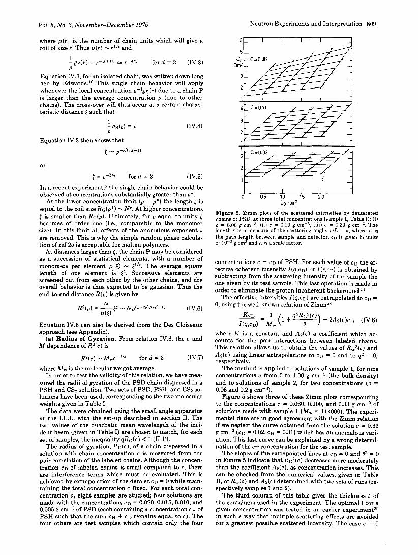
Figure 5. Zimm plots of the scattered intensities by deuterated chains of PSD, at three total concentrations (sample 1, Table I): ( i ) c = 0.06 g ~ m - ~ , (i i) c = 0.10 g ~ r n - ~ , (iii) c = 0.33 g ~ 1 1 3 ~ ~ . The length r is a measure of the scattering angle, r /L = 8, where L is the path length between sample and detector. CD is given in units of lo-* g cm3 and a is a scale factor.

concentrations c - C D of PSH. For each value of CD the effective coherent intensity I(q,cD) or I (~ ,cD) is obtained by subtracting from the scattering intensity of the sample the one given by its test sample. This last operation is made in order to eliminate the proton incoherent background.ll

The effective intensities I(q,cD) are extrapolated to CD = 0, using the well-known relation of ZimmZ8

where K is a constant and A ~ ( c ) a coefficient which ac- counts for the pair interactions between labeled chains, This relation allows US to obtain the values of R&c) and A ~ ( c ) using linear extrapolations to C D = 0 and to q2 = 0, respectively.

The method is applied to solutions of sample 1, for nine concentrations c from 0 to 1.06 g (the bulk density) and to solutions of sample 2, for two concentrations (c = 0.06 and 0.2 g

Figure 5 shows three of these Zimm plots corresponding to the concentrations c = 0.060, 0.100, and 0.33 g emw3 of solutions made with sample 1 (M, = 114000). The experimental data are in good agreement with the Zimm relation if we neglect the curve obtained from the solution c = 0.33 g (CD = 0.02, CH = 0.31) which has an anomalous variation. This last curve can be explained by a wrong determination of the CH concentration for the test sample.

The slopes of the extrapolated lines a t C D = 0 and 82 = 0 in Figure 5 indicate that R c 2 ( c ) decreases more moderately than the coefficient A z ( c ) , as concentration increases. This can be checked from the numerical values, given in Table 11, of R G ( c ) and A ~ ( c ) determined with two sets of runs (respectively samples 1 and 2).

The third column of this table gives the thickness t of the containers used in the experiment. The optimal t for a given concentration was tested in an earlier experiment29 in such a way that multiple scattering effects are avoided for a greatest possible scattered intensity. The case c = 0


Table I1 Concentrations and Radii of Gyration

114000 0.00 10 137 0 6.21 70.8 0.03 10 120 62 3.54 40.4 0.06 10 117 60 1.02 11.6 0.10 5 111 60 0.44 5.0 0.15 5 104 59 0.29 3.3 0.20 2 101 60 0.15 1.7 0.33 2 95 59 0.19 1.0 0.50 1 91 53 0 ? 1.06 1 82 59.5 0 ? (bulk)

500000 0.06 5 242 58 0.11 5.5 0.20 2 226 68 0.03 1.5

111111111111 0 as c g.cm-3 1.00

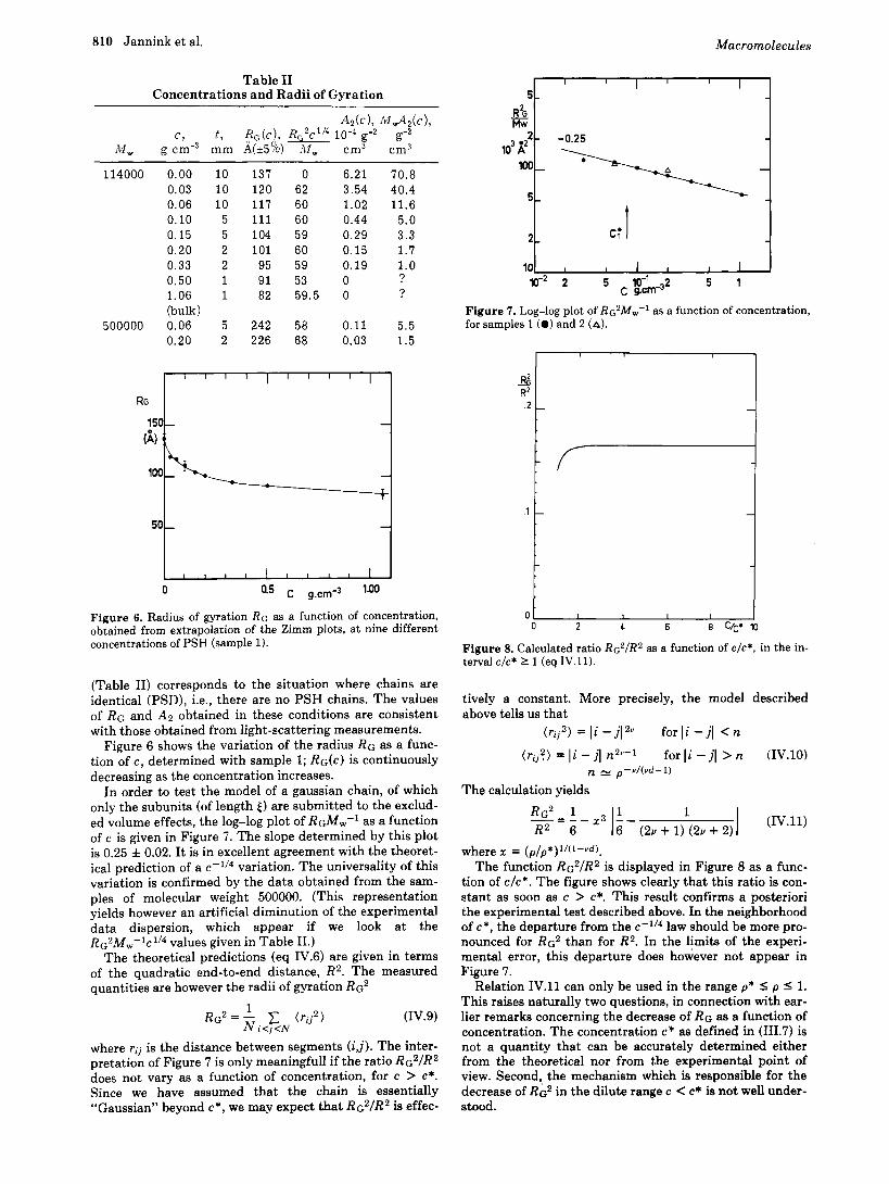
Figure 6. Radius of gyration RG as a function of concentration, obtained from extrapolation of the Zimm plots, a t nine different concentrations of PSH (sample 1).

(Table 11) corresponds to the situation where chains are identical (PSD), Le., there are no PSH chains. The values of RG and A2 obtained in these conditions are consistent with those obtained from light-scattering measurements.

Figure 6 shows the variation of the radius R G as a function of c , determined with sample 1; RG(c) is continuously decreasing as the concentration increases.

In order to test the model of a gaussian chain, of which only the subunits (of length E ) are submitted to the excluded volume effects, the log-log plot of RGM,-' as a function of c is given in Figure 7. The slope determined by this plot is 0.25 f 0.02. It is in excellent agreement with the theoretical prediction of a c-1/4 variation. The universality of this variation is confirmed by the data obtained from the samples of molecular weight 500000. (This representation yields however an artificial diminution of the experimental data dispersion, which appear if we look at the

The theoretical predictions (eq IV.6) are given in terms of the quadratic end-to-end distance, R2. The measured quantities are however the radii of gyration R G ~

values given in Table 11.)

R G ~ =' C ( r i j 2 ) (IV.9) h'i<j<N

where rij is the distance between segments (i,j). The interpretation of Figure 7 is only meaningful1 if the ratio RG2/R2 does not vary as a function of concentration, for c > c*. Since we have assumed that the chain is essentially "Gaussian" beyond c*, we may expect that RG2/R2 is effec-

5 3

- -0.25

- Rb

lo3 f Mw

2

100

5 -

5 lo-' 2 5 1 c g.cm-3 w2 2

Figure 7. Log-log plot of RG~M,.,-' as a function of concentration, for samples 1 (0) and 2 (A).

0 0 2 1 6 8 wc* 10

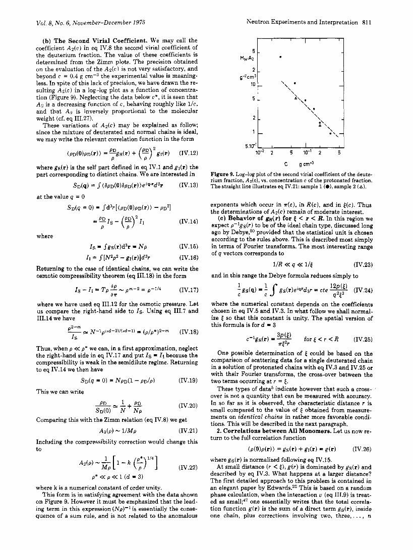
Figure 8. Calculated ratio Rc2/R2 as a function of c/c*, in the interval c/c* 1 1 (eq IV.11).

tively a constant. More precisely, the model described above tells us that

(ri,2) = l i - j 1 2 ~ for t i - j l < n

for Ii - jl > n (r!j?) = Ii - jl n2u--1 (IV.10) n p - v / ( v d - l )

The calculation yields

I (IV.11) I: (21, + 1) (2u + 2) R c ~ 1 1 -- - - - - - 3 -- R2 6

where x = ( p / p * ) l / ( l - Y d ) . The function RG2/R2 is displayed in Figure 8 as a func-

tion of c/c*. The figure shows clearly that this ratio is constant as soon as c > c*. This result confirms a posteriori the experimental test described above. In the neighborhood of c*, the departure from the c-ll4 law should be more pro- nounced for R G ~ than for R2. In the limits of the experimental error, this departure does however not appear in Figure 7.

Relation IV.ll can only be used in the range p* I p I 1. This raises naturally two questions, in connection with earlier remarks concerning the decrease of RG as a function of Concentration. The concentration c y as defined in (111.7) is not a quantity that can be accurately determined either from the theoretical nor from the experimental point of view. Second, the mechanism which is responsible for the decrease of RG2 in the dilute range c < c* is not well under- stood.

Vol. 8, No. 6, November-December 1975 Neutron Experiments and Interpretation 81 1

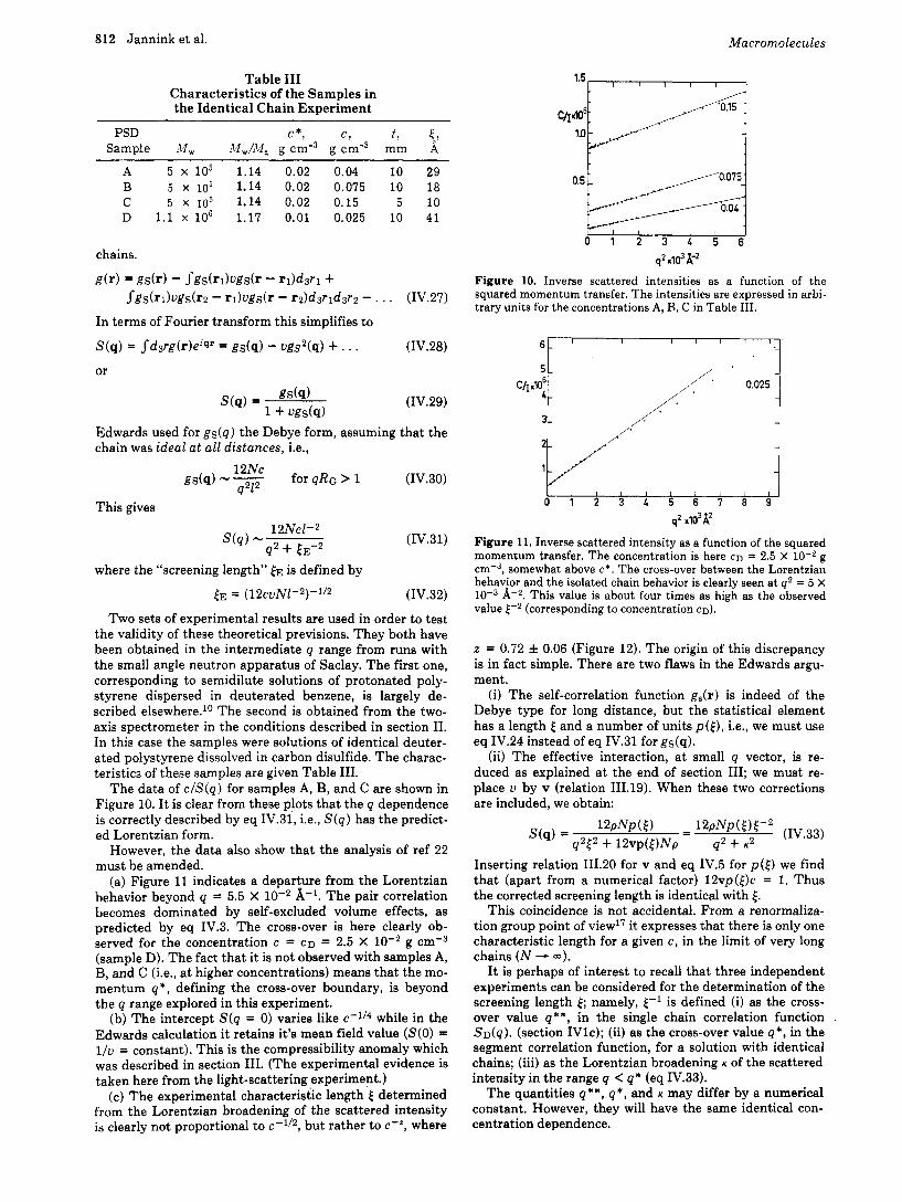
(b) The Second Virial Coefficient. We may call the coefficient Az(c) in eq IV.8 the second virial coefficient of the deuterium fraction. The value of these coefficients is determined from the Zimm plots. The precision obtained on the evaluation of the A ~ ( c ) is not very satisfactory, and beyond c = 0.4 g cm-3 the experimental value is meaning- less. In spite of this lack of precision, we have drawn the resulting A ~ ( c ) in a log-log plot as a function of concentration (Figure 9). Neglecting the data below c*, it is seen that A2 is a decreasing function of c, behaving roughly like l /c, and that A2 is inversely proportional to the molecular weight (cf. eq 111.27).

These variations of A2(c) may be explained as follow; since the mixture of deuterated and normal chains is ideal, we may write the relevant correlation function in the form

where gs(r) is the self part defined in eq IV.l and g d r ) the part corresponding to distinct chains. We are interested in

a t the value q = 0

(IV.14)

where

IS = Sgs(r)d3r = Np (IV. 15)

ZI = S[N2p2 - g1(r)]d3r (IV.16)

Returning to the case of identical chains, we can write the osmotic compressibility theorem (eq 111.18) in the form

I s - ZI I Tp dp pm-2 = p-1/4 (IV.17)

where we have used eq 111.12 for the osmotic pressure. Let us compare the right-hand side to Is. Using eq 111.7 and 111.14 we have

I s

a*

2-m P N-lp(ud-2)/bd-l) (p/p*)2-m (IV.18)

Thus, when p << p* we can, in a first approximation, neglect the right-hand side in eq IV.17 and put I s = I1 because the compressibility is weak in the semidilute regime. Returning to eq IV.14 we then have

(IV.19) s D ( q = 0) = NPDU - PD/P)

This we can write

(IV.20)

Comparing this with the Zimm relation (eq IV.8) we get

AAp) N UMp (IV.21)

Including the compressibility correction would change this to

(IV.22) A2(p) N [ 1 - k ($)'"I MP

p* << p << 1 (d = 3)

where k is a numerical constant of order unity. This form is in satisfying agreement with the data shown

on Figure 9. However it must be emphasized that the lead- ing term in this expression (Np)-' is essentially the conse- quence of a sum rule, and is not related to the anomalous

1 2l 5 .lU1

10-2 2 5 10-1 2 5

c gcm-3

Figure 9. Log-log plot of the second virial coefficient of the deuterium fraction, Az(c), vs. concentration c of the protonated fraction. The straight line illustrates eq Iv.21: sample 1 (O), sample 2 (A).

exponents which occur in a(c) , in R ( c ) , and in [ ( c ) ~ Thus the determinations of A2(c) remain of moderate interest.

< r < R. In this region we expect p-'gs(r) to be of the ideal chain type, discussed long ago by D e b ~ e , ~ O provided that the statistical unit is chosen according to the rules above. This is described most simply in terms of Fourier transforms. The most interesting range of q vectors corresponds to

1/R << q << ll[ (IV.23)

( c ) Behavior of gs(r) for

and in this range the Debye formula reduces simply to 1 -gs(q) = gs(r)eiqrd3r = cte 12po (IV.24) C C 4 *.i2

where the numerical constant depends on the coefficients chosen in eq IV.5 and IV.3. In what follow we shall normal- ize [ so that this constant is unity. The spatial version of this formula is for d = 3

f o r [ < r < R (IV.25)

One possible determination of [ could be based on the comparison of scattering data for a single deuterated chain in a solution of protonated chains with eq IV.3 and IV.25 or with their Fourier transforms, the cross-over between the two terms occurring a t r = [.

These types of data5 indicate however that such a cross- over is not a quantity that can be measured with accuracy. In so far as it is observed, the characteristic distance r is small compared to the value of [ obtained from measurements on identical chains in rather more favorable conditions. This will be described in the next paragraph.

2. Correlations between All Monomers. Let us now re- turn to the full correlation function

(p(O)p(r ) ) = gs(r) + g d r ) = g(r ) (IV.26)

where gs(r) is normalized following eq IV.15. At small distance (r < [), g(r) is dominated by gs(r) and

described by eq IV.3. What happens at a larger distance? The first detailed approach to this problem is contained in an elegant paper by Edwards.22 This is based on a random phase calculation, when the int,eraction u (eq 111.9) is treat- ed as ~ma11;~7 one essentially writes that the total correlation function g ( r ) is the sum of a direct term gs(r) , inside one chain, plus corrections involving two, three,. . . , n

812 Jannink et al.

Table I11 Characteristics of the Samples in the Identical Chain Experiment

Macromolecules

1.5 I I I I I I

t A

A 5 x l o 5 1.14 0.02 0.04 10 29 B 5 x lo5 1.14 0.02 0.075 10 18 C 5 x io5 1.14 0.02 0.15 5 10 D 1.1 x lo6 1.17 0.01 0.025 10 41

chains.

g ( r ) = g d r ) - Sgs(rl)ugs(r - r d d m +

In terms of Fourier transform this simplifies to

S(q) = Jd3rg(r)eiqr = gs(q) - ugs2(q) + . . . or

Sgs ( rhgs ( r2 - rl)ugs(r - rdd3nd3r2 - . . . (IV.27)

(IV.28)

(IV.29)

Edwards used for gs(q) the Debye form, assuming that the chain was ideal a t all distances, Le.,

12Nc gs(q) - - for q R G > 1 (IV.30)

q 2 1 2 This gives

(IV.31)

where the “screening length” f~ is defined by

EE = (12~uN1-~)-’/~ (IV.32)

Two sets of experimental results are used in order to test the validity of these theoretical previsions. They both have been obtained in the intermediate q range from runs with the small angle neutron apparatus of Saclay. The first one, corresponding to semidilute solutions of protonated polystyrene dispersed in deuterated benzene, is largely described elsewhere.1° The second is obtained from the two- axis spectrometer in the conditions described in section 11. In this case the samples were solutions of identical deuterated polystyrene dissolved in carbon disulfide. The characteristics of these samples are given Table 111.

The data of c / S ( q ) for samples A, B, and C are shown in Figure 10. I t is clear from these plots that the q dependence is correctly described by eq IV.31, i.e., S(q ) has the predicted Lorentzian form.

However, the data also show that the analysis of ref 22 must be amended.

(a) Figure 11 indicates a departure from the Lorentzian behavior beyond q = 5.5 X 10-2 A-1. The pair correlation becomes dominated by self-excluded volume effects, as predicted by eq IV.3. The cross-over is here clearly observed for the concentration c = CD = 2.5 X g cmw3 (sample D). The fact that it is not observed with samples A, B, and C (i.e., a t higher concentrations) means that the momentum q* , defining the cross-over boundary, is beyond the q range explored in this experiment.

(b) The intercept S(q = 0) varies like c-1/4 while in the Edwards calculation it retains it’s mean field value (S(0) = l / u = constant). This is the compressibility anomaly which was described in section 111. (The experimental evidence is taken here from the light-scattering experiment.)

(c) The experimental characteristic length f determined from the Lorentzian broadening of the scattered intensity is clearly not proportional to cT1l2, but rather to c-*, where

0.5

0 1 2 3 6 5 6

q 2 .Id A-2

Figure 10. Inverse scattered intensities as a function of the squared momentum transfer. The intensities are expressed in arbitrary units for the concentrations A, B, C in Table 111.

6 I l l I / I I l I

51

2 I II. / ’ 0.025 1

I

1 I I I I I I I I I I /

0 1 2 3 4 5 6 7 8 9

q2 x103A2

Figure 11. Inverse scattered intensity as a function of the squared momentum transfer. The concentration is here CD = 2.5 X g ~ m - ~ , somewhat above c*. The cross-over between the Lorentzian behavior and the isolated chain behavior is clearly seen a t q2 = 5 X

A-2. This value is about four times as high as the observed value E - 2 (corresponding to concentration CD).

z = 0.72 f 0.06 (Figure 12). The origin of this discrepancy is in fact simple. There are two flaws in the Edwards argument.

(i) The self-correlation function g,(r) is indeed of the Debye type for long distance, but the statistical element has a length f and a number of units p ( f ) , Le., we must use eq IV.24 instead of eq IV.31 for gs(q).

(ii) The effective interaction, a t small q vector, is reduced as explained a t the end of section 111; we must replace u by v (relation 111.19). When these two corrections are included, we obtain:

Inserting relation 111.20 for v and eq IV.5 for p ( f ) we find that (apart from a numerical factor) lPvp(f)c = 1. Thus the corrected screening length is identical with 5.

This coincidence is not accidental. From a renormalization group point of view17 it expresses that there is only one characteristic length for a given c, in the limit of very long chains ( N - a).

I t is perhaps of interest to recall that three independent experiments can be considered for the determination of the screening length 5; namely, f - l is defined (i) as the cross- over value q** , in the single chain correlation function S D ( q ) . (section Ivlc) ; (ii) as the cross-over value q * , in the segment correlation function, for a solution with identical chains; (iii) as the Lorentzian broadening K of the scattered intensity in the range q < q* (eq IV.33).

The quantities q * * , q* , and K may differ by a numerical constant. However, they will have the same identical concentration dependence.


10

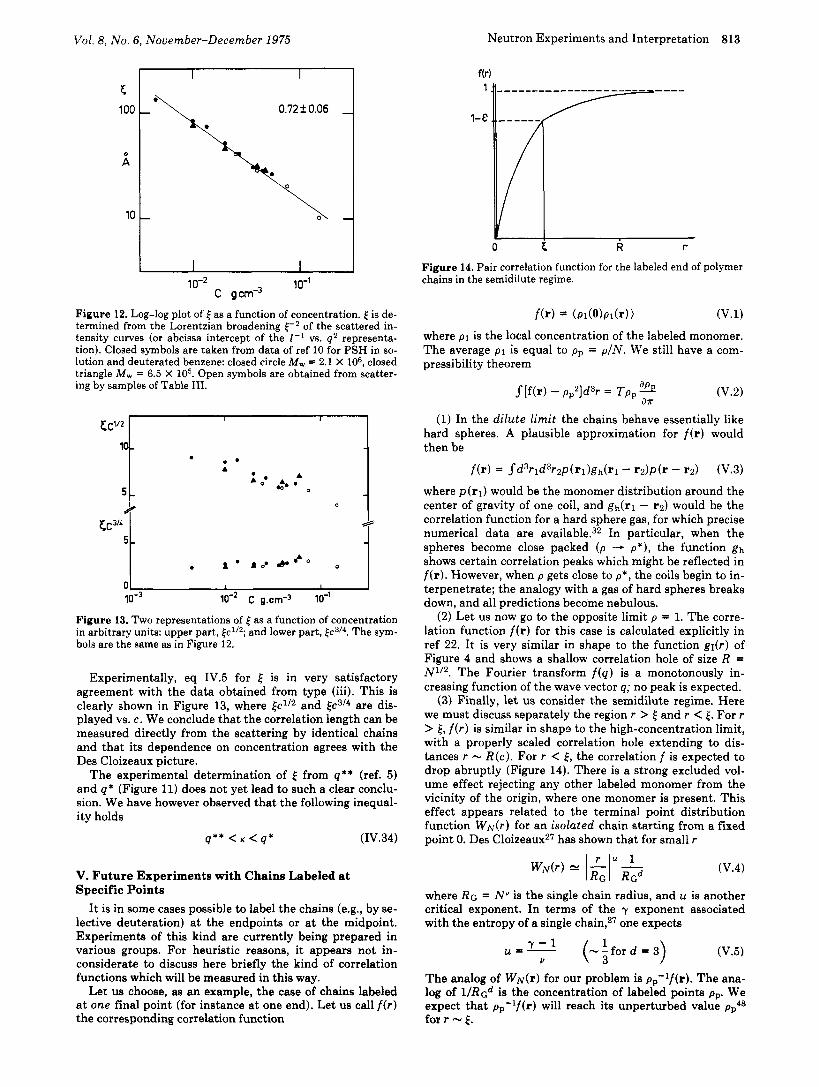
Figure 12. Log-log plot of [ as a function of concentration. [ is determined from the Lorentzian broadening of the scattered intensity curves (or abcissa intercept of the I-’ vs. q 2 representation). Closed symbols are taken from data of ref 10 for PSH in solution and deuterated benzene: closed circle M , = 2.1 x IO6, closed triangle M , = 6.5 X lo5. Open symbols are obtained from scattering by samples of Table 111.

cc’’l I I

10-~ IO-* c g.cm-3 IO-’

Figure 13. Two representations of [ as a function of concentration in arbitrary units: upper part, [ c ~ ’ ~ ; and lower part, [c3I4. The symbols are the same as in Figure 12.

Experimentally, eq IV.5 for is in very satisfactory agreement with the data obtained from type (iii). This is clearly shown in Figure 13, where and kc3/* are displayed vs. c. We conclude that the correlation length can be measured directly from the scattering by identical chains and that its dependence on concentration agrees with the Des Cloizeaux picture.

The experimental determination of k from q** (ref. 5) and q* (Figure 11) does not yet lead to such a clear conclu- sion. We have however observed that the following inequality holds

q** < K < q* (IV.34)

V. Future Experiments with Chains Labeled at Specific Points

I t is in some cases possible to label the chains (e.g., by se- lective deuteration) a t the endpoints or a t the midpoint. Experiments of this kind are currently being prepared in various groups. For heuristic reasons, it appears not in- considerate to discuss here briefly the kind of correlation functions which will be measured in this way.

Let us choose, as an example, the case of chains labeled a t one final point (for instance a t one end). Let us call f ( r ) the corresponding correlation function

0 R r

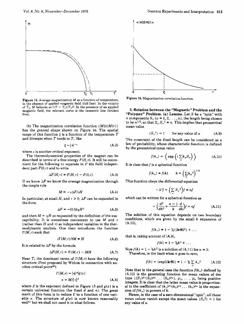
Figure 14. Pair correlation function for the labeled end of polymer chains in the semidilute regime.

f ( r ) = (m(O)pl(r)) (V.1)

where p1 is the local concentration of the labeled monomer. The average p1 is equal to p p = p / N . We still have a compressibility theorem

(1) In the dilute limit the chains behave essentially like hard spheres. A plausible approximation for f ( r ) would then be

f(r) = Sd3r1d3r2p(r l )ghh - rz)p(r - 1 2 ) (V.3)

where p(r1) would be the monomer distribution around the center of gravity of one coil, and gh(r1 - 12) would be the correlation function for a hard sphere gas, for which precise numerical data are available.32 In particular, when the spheres become close packed ( p - p * ) , the function g h shows certain correlation peaks which might be reflected in f ( r ) . However, when p gets close to p * , the coils begin to interpenetrate; the analogy with a gas of hard spheres breaks down, and all predictions become nebulous.

(2) Let us now go to the opposite limit p = 1. The correlation function f ( r ) for this case is calculated explicitly in ref 22. It is very similar in shape to the function gI(r) of Figure 4 and shows a shallow correlation hole of size R = N1l2. The Fourier transform f ( q ) is a monotonously in- creasing function of the wave vector q; no peak is expected.

(3) Finally, let us consider the semidilute regime. Here we must discuss separately the region r > and r < E . For r > 4, f ( r ) is similar in shap2 to the high-concentration limit, with a properly scaled correlation hole extending to distances r - R(c ) . For r < k , the correlation f is expected to drop abruptly (Figure 14). There is a strong excluded volume effect rejecting any other labeled monomer from the vicinity of the origin, where one monomer is present. This effect appears related to the terminal point distribution function WN(r) for an isolated chain starting from a fixed point 0. Des CloizeauxZ7 has shown that for small r

where RG = N u is the single chain radius, and u is another critical exponent. In terms of the y exponent associated with the entropy of a single chain,27 one expects

V (-:ford = 3 Y - 1 u=- W.5)

The analog of W d r ) for our problem is pP-lf(r) . The analog of l/Rcd is the concentration of labeled points pp. We expect that pp-lf(r) will reach its unperturbed value pp4S for r - E .


Thus we are led to the following conjecture

Measurements in this domain are not easy. But, if they can be performed in the future, they may give direct infor- mation on the exponent y.

Similar experiments can be considered with the chains labeled a t their midpoint, or also with chains labeled a t both ends. The correlation function fdr) for the latter case is qualitatively reproduced on Figure 14.

VI. Concluding Remarks 1. Deviations from Mean Field. We hope to have

shown that (a) semidilute solutions show significant deviations from the mean field theory and that (b) the deviations can be systematized in terms of one single scaling assumption (say for the osmotic pressure). We also conclude that the apparently very different points of view introduced by Des Cloizeaux and Edwards can be reconciled provided certain renormalizations (of the chain statistical unit, and of the interactions) are included in the Edwards picture.

Certain points remain obscure; the data on the heats of dilution do not fit with the scaling law, probably because they are not taken in a broad enough semidilute concentration range. Also the experimental behavior of the intrachain correlation function gs(r) (as measured on deuterated chains) does not show clearly the cross-over at r = E which is expected. On the other hand, the cross-over observed for the segment pair correlation function, measured on identical chains, occurs a t a distance r which is smaller than E. But the three independent neutron (plus the light scattering) data on the anomalous exponent do converge remarkably to the same value and are in good agreement with the Flory calculation of Y.

All our discussion has been very qualitative, and primari- ly oriented toward the determination of certain power laws. We have not investigated, experimentally or theoretically, the constant factors which enter in these power laws; comparing with the present experience in the field of phase transition,S4 we are let to believe that measurements of these prefactors will require long efforts.

2. Future Investigations with Poor Solvents. Another direction of interest is related to controlled changes of the interaction constant u. In all our discussion we have taken u to be positive and comparable to the monomer volume, as it is in a good solvent. When the solvent quality decreases, and we get close to a 8 point, the interaction constant and u become small and the next virial term in the free energy (eq 111.8) must be included. One of us has argued recently that the region T - 8 is related to ,a point in the magnetic analog.33 This leads (for T = 8 exactly) to an osmotic pressure law in the semidilute regime (at d = 3), ?r = c3, essentially identical with the mean field prediction for T = 8. For T < 8 the demixtion problem is still a challenge (see Appendix), but the complications introduced by polydispersity (even if the latter is weak) may forbid precise determinations of the associated critical exponents.

3. A Conjecture on t h e Rubber Elasticity of Entan- gled Chains. Returning to the good solvent situation, it may be appropriate to insert in these conclusions one remark and one conjecture. The remark concerns the osmotic pressure law ?r N Tc914 in the semidilute regime. It may be argued quite generally that (apart from a numerical coefficient) ?r/T measures the number of contact points between different chains (per unit volume). In a mean field picture this number is proportional to p2. Here, as explained in section 111, it is smaller than p2.

This may possibly be related to an interesting physical parameter; if we measure the viscoelastic properties of a solution, at a finite but low-frequency w , and if the chains are long enough (so that the relaxation rate is smaller than w ) we expect to find an elastic modulus E of the rubber type, due only to entanglements between different chains. A number of arguments suggests that E/T is proportional to the number of contact points; in mean field theory this would give E = Tp2. More complicated power laws have been proposed within mean field theory35 but they are open to some criticism.36 Our conjecture is that E is indeed proportional to the exact density of contact points, i.e., that

E = Tp914 (p* << p << 1)

The experimental situation is not too clear a t present, but we hope to come back to this point in later studies. 4. Semidilute Behavior of Two-Dimensional Polymer

Films. Monomolecular polymer films can be prepared on a liquid interface, or on a solid substrate. In principle, for d = 2 the deviations from mean field are much more glazing; for instance the osmotic pressure should behave like c3 in good solvent conditions, rather than c2. However, the range of semidilute concentrations is not very broad in two dimensions. Also, many experimental techniques (such as neutron scattering) become inapplicable for a single film. It would be necessary to work with a system of many super- posed films, for instance, to incorporate solute polymer chains in a lamellar phase of lipid plus water,37 each lamel- la behaving more or less like an independent two-dimensional sheet. Clearly these experiments belong to a rather remote future.

Acknowledgment. We wish to thank Des Cloizeaux, Boccara, Strazielle, Bidaux, and Mirkovitch for stimulating discussions over this subject; Decker, Herbert, and Rempp for their cooperation in the deuteration of the molecules; and Higgins, Nierlich, BouB, and Ober for preparing the data processing.

Appendix The Magnetic Analog to Polymer Solution. An Intro-

duction. In this appendix we present a new and perhaps simpler d e r i v a t i ~ n ~ ~ of the analogy found by de Gennes26 and Des Cloiseaux6 between the “polymer” problem and a “magnetic” problem.

1. A Few Basic Facts about Ferromagnets. The main features of ferromagnetic transitions are reviewed for instance in the book by Stanley.39 Ferromagnetic order is de- scribed49 by a magnetization vector M with a certain number n of independent componants: n may be equal to 3 (Heisenberg magnets), to 2 (planar), or to 1 (Ising magnets).

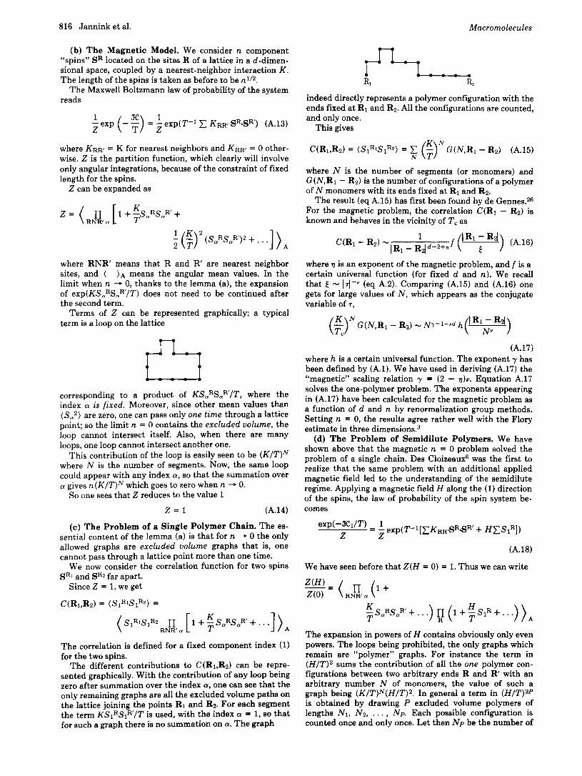
The average magnetization M of the magnet is a function of the temperature T and of the applied magnetic field H . In zero field and a t high T , the magnetization M vanishes. However, below a certain critical temperature T , there is a spontaneous magnetization M( T,H = 0) as shown in Figure 15. Coming toward the critical point from the high-temperature side ( T > T,, H = 0) the proximity of a transition is signalled by two main effects.

(a) The susceptibility x = ( a M / a H ) l ~ = o becomes large and diverges at T,

(A.1)

y is a certain critical exponent, depending only on d (the dimensionality) and on n (the number of components of M). Approximate formulas for y (d = 3,n) have now been worked 0 ~ t . l ~


f M 1

\ I I

t - 0 z r 0 Tc TI T

Figure 15. Average magnetization M as a function of temperature, in the absence of applied magnetic field (full line). In the vicinity of T,, A4 behaves as ((T - Tc)/Tc)o. In the presence of an applied magnetic field, the relevant curve is the isometric line (broken line).

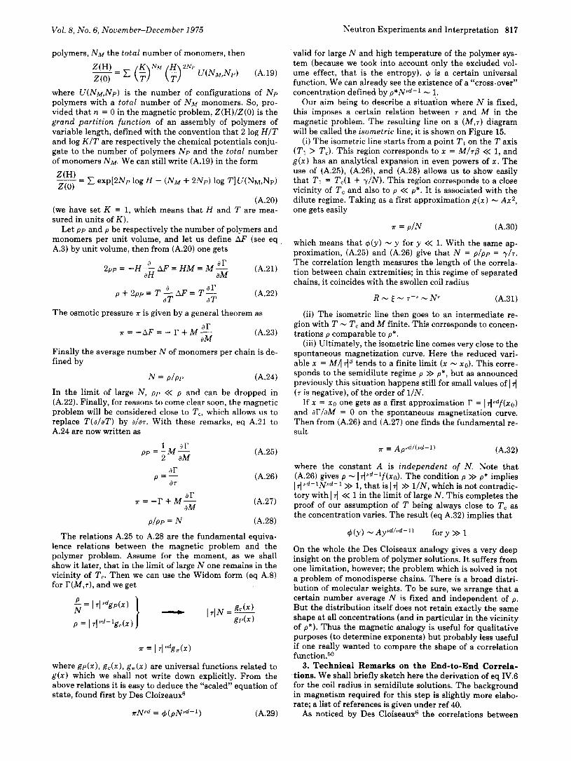
(b) The magnetization correlation function ( M ( O ) M ( r ) ) has the general shape shown on Figure 16. The spatial range of this function E is a function of the temperature T and diverges when T tends to T , like

E-ld-” (A.2)

where u is another critical exponent. The thermodynamical properties of the magnet can be

described in terms of a free energy F(H,T) . It will be convenient for the following to separate in F the field independent part F(0,r) and to write

AF(H,T) = F ( H , r ) - F ( ~ , T ) (A.3)

If we know AF we know the average magnetization through the simple rule

M = -aAFlaH 64.4)

In particular, a t small H, and T > 0, AF can be expanded in the form

A F = -(0.5)xH2 (A.5)

Figure 16. Magnetization correlation function.

2. Relation between the “Magnetic” Problem and the “Polymer” Problem. (a) Lemma. Let S be a “spin” with n components Sa (a = 1 , 2 , . . . , n ) , the length being chosen to be n1I2, so that 2, Sa2 = n. This implies that geometrical mean value

(-4.9) The constraint of the fixed length can be considered as a law of probability, whose characteristic function is defined by the geometrical mean value

(S,2) = 1 for any value of LY

I t is clear that f is a spherical function

k = (Fk,Z)1’2

This function obeys the differential equation

which can be written for a spherical function as

- ( f + s 2 L ) f = n f k dk

(A.lO)

( A . l l )

and then M = x H as requested by the definition of the SUS-

ceptibility. It is sometimes convenient to use M and (rather than H and T ) as independent variables in the ther-

The solution of this equation depends on two boundary conditions, which are given by the small k expansion of (A*10),

f(k,) = 1 - $( (k*S)’) + . . modynamic analysis. One then introduces the function r (M,T) such that

ar(M,r) /6M = H (A.6) that is, taking account of (A.9),

. . f (k) = 1 - %k2 + . . .

I t is related to AF by the formula Now f ( k ) = 1 - Kk2 is a solution of ( A . l l ) for n = 0.

A F ( H , r ) r ( M , T ) - M H (A.7) Therefore, in the limit when n goes to zero, Near T, the dominant terms of I’(M,T) have the following structure (first proposed by Widom in connection with another critical point40)

r ( M , T ) = I . fydg(x)

x = M A r 1 @ (A.8) where ,f3 is the exponent defined in Figure 15 and g ( x ) is a certain universal function (for fixed d and n). The great merit of this form is to reduce r to a function of one variable x . The structure of g ( x ) is now known reasonably wel141 but we shall not need it in what follows.

f ( k ) = (exp(ik*S)) = 1 - K E ka2 (A.12)

Note that in the general case the function f(k,) defined by (A.lO) is the generating function for mean values of the type ((Si)P*(S2)pz . . . (Sn)Pn), p1, . . . , pn being positive integers. It is clear that the latter mean value is proportional to the coefficient of (kl)Pl(kz)PZ. . . (k,)Pn in the expansion of f ( k , ) in powers of k.

Hence, in the case of a zero-dimensional “spin”, all these mean values vanish except the mean values ( S o 2 ) = 1 for any value of a.

a


(b) T h e Magnetic Model. We consider n component “spins” SR located on the sites R of a lattice in a d-dimensional space, coupled by a nearest-neighbor interaction K. The length of the spins is taken as before to be n1I2.

The Maxwell Boltzmann law of probability of the system reads

where KRR, = K for nearest neighbors and KRR = 0 other- wise. Z is the partition function, which clearly will involve only angular integrations, because of the constraint of fixed length for the spins.

Z can be expanded as

K RNR

where RNR’ means that R and R’ are nearest neighbor sites, and ( ) A means the angular mean values. In the limit when n - 0, thanks to the lemma (a), the expansion of exp(KSORSoR’/T) does not need to be continued after the second term.

Terms of Z can be represented graphically; a typical term is a loop on the lattice

corresponding to a product of KSORSaR’/T, where the index a is fixed. Moreover, since other mean values than ( ScY2) are zero, one can pass only one time through a lattice point; so the limit n = 0 contains the excluded volume, the loop cannot intersect itself. Also, when there are many loops, one loop cannot intersect another one.

where N is the number of segments. Now, the same loop could appear with any index a, so that the summation over a gives n(K/T)N which goes to zero when n - 0.

This contribution of the loop is easily seen to be

So one sees that Z reduces to the value 1

z = 1 (A.14)

(e) The Problem of a Single Polymer Chain. The es- sential content of the lemma (a) is that for n + 0 the only allowed graphs are excluded volume graphs that is, one cannot pass through a lattice point more than one time.

We now consider the correlation function for two spins SRl and SR2 far apart.

Since 2 = 1, we get

C(R1,Rz) = (SlR1SlR2) =

The correlation is defined for a fixed component index (1) for the two spins.

The different contributions to C(R1,Rz) can be represented graphically. With the contribution of any loop being zero after summation over the index a, one can see that the only remaining graphs are all the excluded volume paths on the lattice joining the points R1 and Rz. For each segment the term KSIRSIR’/T is used, with the index a = 1, so that for such a graph there is no summation on a. The graph

I,,,_ R,

indeed directly represents a polymer configuration with the ends fixed at R1 and R2. All the configurations are counted, and only once.

This gives

K N C(R1,Rd = (SlR1SlR2) = (T) G(N,R1 - Rz) (A.15)

where N is the number of segments (or monomers) and G(N,R1 - R2) is the number of configurations of a polymer of N monomers with its ends fixed a t R1 and R2.

The result (eq A.15) has first been found by de Gennes.26 For the magnetic problem, the correlation C(R1 - R2) is known and behaves in the vicinity of T, as

N

where 7 is an exponent of the magnetic problem, and f is a certain universal function (for fixed d and n). We recall that E N Id -v (eq A.2). Comparing (A.15) and (A.16) one gets for large values of N, which appears as the conjugate variable of 7,

(A.17) where h is a certain universal function. The exponent y has been defined by (A.1). We have used in deriving (A.17) the “magnetic” scaling relation y = (2 - 7)v. Equation A.17 solves the one-polymer problem. The exponents appearing in (A.17) have been calculated for the magnetic problem as a function of d and n by renormalization group methods. Setting n = 0, the results agree rather well with the Flory estimate in three dimension^.^

(d) The Problem of Semidilute Polymers. We have shown above that the magnetic n = 0 problem solved the problem of a single chain. Des Cloizeaux6 was the first to realize that the same problem with an additional applied magnetic field led to the understanding of the semidilute regime. Applying a magnetic field H along the (1) direction of the spins, the law of probability of the spin system becomes

(A.18)

We have seen before that Z(H = 0) = 1. Thus we can write

> > A ; S,RS,R‘ + . . .) g (1 + 7 S 1 R + . . . H

The expansion in powers of H contains obviously only even powers. The loops being prohibited, the only graphs which remain are “polymer” graphs. For instance the term in

sums the contribution of all the one polymer configurations between two arbitrary ends R and R’ with an arbitrary number N of monomers, the value of such a graph being (K/T)N(H/T)2. In general a term in is obtained by drawing P excluded volume polymers of lengths N1, N2, . . . , Np. Each possible configuration is counted once and only once. Let then N p be the number of

Vol. 8, No . 6, November-December 1975 Neutron Experiments and Interpretation 817

polymers, NM the total number of monomers, then

where U ( N M , N ~ ) is the number of configurations of N p polymers with a total number of NM monomers. So, provided that n = 0 in the magnetic problem, Z(H)/Z(O) is the grand parti t ion funct ion of an assembly of polymers of variable length, defined with the convention that 2 log HIT and log KIT are respectively the chemical potentials conjugate to the number of polymers Np and the total number of monomers NM. We can still write (A.19) in the form

-- ‘(HI - E exp[2Np log H - (NM + 2Np) log T]U(NM,NP) Z(0)

(A.20) (we have set K = 1, which means that H and T are measured in units of K ) .

Let p p and p be respectively the number of polymers and monomers per unit volume, and let us define AF (see eq A.3) by unit volume, then from (A.20) one gets

a ar 2pp = -H- AF = H M = M -

aH aM (A.21)

a ar aT aT

p + 2 p p = T - A F = T - (A.22)

The osmotic pressure P is given by a general theorem as ar

P = -AF = - r + M - aM

(A.23)

Finally the average number N of monomers per chain is defined by

N = p l p p (A.24)

In the limit of large N , p p << p and can be dropped in (A.22). Finally, for reasons to come clear soon, the magnetic problem will be considered close to T,, which allows us to replace T(alaT) by alar. With these remarks, eq A.21 to A.24 are now written as

1 ar 2 aM

p p = - M -

ar P = -

a7

ar P = - r + ~ - aM

(A.25)

(A.26)

(A.27)

p l p p = N (A.28)

The relations A.25 to A.28 are the fundamental equiva- lence relations between the magnetic problem and the polymer problem. Assume for the moment, as we shall show it later, that in the limit of large N one remains in the vicinity of T,. Then we can use the Widom form (eq A.8) for r ( M , 7 ) , and we get

7T = I TI ydg,(x)

where g p ( x ) , g,(x), g,(x) are universal functions related to g ( x ) which we shall not write down explicitly. From the above relations it is easy to deduce the “scaled” equation of state, found first by Des Cloizeaux6

aNYd = &(pNYd-l) (A.29)

valid for large N and high temperature of the polymer system (because we took into account only the excluded volume effect, that is the entropy). 4 is a certain universal function. We can already see the existence of a “cross-over’’ concentration defined by p*NYd-l - 1.

Our aim being to describe a situation where N is fixed, this imposes a certain relation between T and M in the magnetic problem. The resulting line on a (M,T) diagram will be called the isometric line; it is shown on Figure 15.

(i) The isometric line starts from a point T I on the T axis ( T I > T,). This region corresponds to x = MITP << 1, and g(x) has an analytical expansion in even powers of 3c. The use of (A.25), (A.26), and (A.28) allows us to show easily that T I = T,(1 + TIN). This region corresponds to a close vicinity of T , and also to p << p*. I t is associated with the dilute regime. Taking as a first approximation g ( x ) - Ax2 , one gets easily

P = PIN (A.30)

which means that d ( y ) - y for y << 1. With the same approximation, (A.25) and (A.26) give that N = p / p p = Y / T . The correlation length measures the length of the correlation between chain extremities; in this regime of separated chains, it coincides with the swollen coil radius

R - E - 7-” -w (A.31)

(ii) The isometric line then goes to an intermediate region with T - T , and M finite. This corresponds to concentrations p comparable to p*.

(iii) Ultimately, the isometric line comes very close to the spontaneous magnetization curve. Here the reduced variable x = M/l d B tends to a finite limit ( x - x ~ ) . This corresponds to the semidilute regime p >> p * , but as announced previously this situation happens still for small values of 14 ( T is negative), of the order of 1/N.

If x = x o one gets as a first approximation r = I d y d f ( x 0 )

and arlaM = 0 on the spontaneous magnetization curve. Then from (A.26) and (A.27) one finds the fundamental result

(A.32)

where the constant A is independent of N. Note that (A.26) gives p - I 4 ” d - 1 f ( ~ o ) . The condition p >> p* implies 14 ud-lNvd-l >> 1, that is 14 >> 1/N, which is not contradic- tory with 14 << 1 in the limit of large N . This completes the proof of our assumption of T being always close to T , as the concentration varies. The result (eq A.32) implies that

A = A u d l ( v d - I ) P

4 ( y ) - AyUdlvd - l ) for y >> 1

On the whole the Des Cloiseaux analogy gives a very deep insight on the problem of polymer solutions. I t suffers from one limitation, however; the problem which is solved is not a problem of monodisperse chains. There is a broad distribution of molecular weights. To be sure, we arrange that a certain number average N is fixed and independent of p . But the distribution itself does not retain exactly the same shape a t all concentrations (and in particular in the vicinity of p * ) . Thus the magnetic analogy is useful for qualitative purposes (to determine exponents) but probably less useful if one really wanted to compare the shape of a correlation function.50

3. Technical Remarks on the End-to-End Correla- tions. We shall briefly sketch here the derivation of eq IV.6 for the coil radius in semidilute solutions. The background in magnetism required for this step is slightly more elabo- rate; a list of references is given under ref 40.

As noticed by Des Cloiseaux6 the correlations between


two ends of one same chain correspond to transverse correlations in the magnetic problem; if the applied field H is along the z axis, we look at (Mx(0)Mx(r)) or at it’s Fourier transform (lMx(q)12). This has the form39

where A varies as kq where 7 is another critical exponent, defined as in ref 39. The quantity ~ 1 - l is a characteristic lengthF1 and will give us the size of the coils. The quantity A/K12 is proportional to the transverse magnetic susceptibility which is ~ i m p l ? ~

XJ. = MoIH (A.34)

Mo being the spontaneous magnetization. We can eliminate H through eq A.21 obtaining

~ 1 ’ ( A I M o 2 ) p p

Using the scaling law for E and Mo, and various relations between critical exponents, plus eq A.26 to eliminate 7 in terms of p we get

(A.35)

an equation equivalent to (IV.7). Similar arguments can be applied to the discussion of the

long-range correlation hole (shown on Figure 14) in semidilute systems. What is considered here is the correlations between the ends of all chains which, as shown in ref 6, is related to longitudinal correlations or susceptibilities.

However, for a magnetic system with n # 1, these longitudinal susceptibilities are influenced by transverse fluctuations; an early discussion of this point can be found in ref 42. It is possible to show for instance that in three space dimensions the longitudinal ‘correlation function contains a long-range term

(A.36) 1 1 Mo2F2“ r2

(6Mz(0)6Mz(r)) N --e-ZKr

This is the source of the correlation hole (extending to distances of order of R) . More precise calculation of the hole cannot be attempted from this approach because of the polydispersity effect discussed above; the R.P.A. approach of ref 25 is probably preferable here.

References and Notes (1) (a) Laboratoire U o n Brillouin, Centre d’Etudes NuclCaires de Saclay;

(b) Centre de Recherches sur les MacromolBcules; (c) CollBge de France.

(2) (a) P. J. Flory, J. Chem. Phys., 10, 51 (1942); (b) M. L. Huggins, J. Phys. Chem., 46.51 (1942).

(3) P. J. Flory, “Principles of Polymer Chemistry”, Cornell University Press, Ithaca, N.Y., 1967.

(4) J. P. Cotton, B. Farnoux, and G. Jannink, J. Chem. Phys., 57, 290 (1972).

(5) B. Farnoux, M. Daoud, D. Decker, G. Jannink, and R. Ober, J. Phys. (Paris) Lett., 36, L35 (1975).

(6) J. Des Cloizeaux, J. Phys. (Paris), 36,281 (1975). ( 7 ) I. I. Gurevitch and L. V. Tarasov, “Low Energy Neutron Physics”,

North-Holland Publishing Co., Amsterdam, 1968.

(8) J. P. Cotton, B. Farnoux, G. Jannink, J. Mons, and C. Picot, C. R.

(9) R. G. Kirste, W. A. Kruse, and J. Schelten, Makromol. Chem , 162,299 Hebd. Seances Acad. Sci., Ser. C, 275,175 (1972).

(1972). (10) J. P. Cotton, These Universit.6 Paris VI, 1973; CEA, No. 1743. (11) J. P. Cotton, D. Decker, H. Benoit, B. Farnoux, J. Higgins, G. Jannink,

R. Ober, C. Picot, and J. Des Cloizeaux, Macromolecules, 7,863 (1974). (12) W. H. Stockmayer, Makromol. Chem., 35,54 (1960). (13) C. Loucheux, G. Weil, and H. Benoit, J . Chim. Phys., 43,540 (1958). (14) C. Domb, J. Gillis, and G. Wilmers, Proc. Phys. SOC., London, 85,625

(15) M. E. Fisher, J. Chem. Phys., 44,616 (1966). (16) S. F. Edwards, Proc. Phys. Soc., London, 85,613 (1965). (17) S.-K. Ma, Reo. Mod. Phys., 45,589 (1973). (18) J. P. Cotton, B. Farnoux, G. Jannink, and C. Strazielle, J . Polym. Sci.,

(19) G. Gee and W. J. Orr, Trans. Faraday SOC., 42,507 (1946). (20) P. A. Egelstaff, “An Introduction to the Liquid State”, Academic

(21) H. Benoit and C. Picot, Pure Appl. Chem., 12,545 (1966). (22) S. F. Edwards, Proc. Phys. SOC., London, 88,265 (1966). (23) R. G. Kirste, W. A. Kruse, and K. Ibel, Polymer, 16,120 (1975). (24) D. G. Ballard, J. Schelten, and G. D. Wignall, Eur. Polym. J., 9, 965

(25) P. G. de Gennes, J. Phys. (Paris), 31,235 (1970). (26) P. G. de Gennes, Phys. Lett. A, 38,339 (1972). (27) J. Des Cloizeaux, J. Phys. (Paris), 31,715 (1970). (28) B. H. Zimm, J. Chem. Phys., 16,1093 (1948). (29) J. P. Cotton, D. Decker, B. Farnoux, G. Jannink, and R. Ober, Phys.

(30) P. Debye, J. Phys. Colloid. Chem., 51,18 (1947). (31) G. Jannink and P. G. de Gennes, J. Chem. Phys., 48,2260 (1968). (32) J. 0. Hirschfelder, C. F. Curtis, and R. B. Bird, “Molecular Theory of

Gases and Liquids”, Wiley, New York, N.Y., 1954. (33) P. G. de Gennes, J. Phys. (Paris), Lett., 36, L55 (1975). (34) P. Heller, Rep. Prog. Phys., 30,731 (1967). (35) S. F. Edwards, Proc. Phys. SOC., London, 92,9 (1967). (36) P. G. de Gennes, to be published. (37) P. G. de Gennes, to be published. (38) G. Sarma, Lecture Notes Saclay, 1974, unpublished. (39) H. E. Stanley, “Introduction to Phase Transition and Critical Phenom-

ena”, Oxford University Press, London, 1971. (40) B. Widom, J. Chem. Phys., 43,3898 (1965). (41) M. E. Fisher, Rep. Prog. Phys., 30,615 (1967). (42) P. G. de Gennes, “Magnetism”, Vol. 111, G. T. Rad0 and H. Suhl, Ed.,

Academic Press, New York, N.Y., 1963. (43) To avoid cumbersome factors in the theoretical discussions, we shall

consider our molecules as inscribed in a periodic lattice, as in the Flory- Huggins model, and we shall take the lattice parameter 1 as our unit of length. The concentration of polymer chains, pp (number of chains per unit volume), is then a dimensionless number going from 0 (pure solvent) to 1JN (molten polymer). The concentration of monomers, p, is then equal to the polymer volume fraction. Whenever experimental results are discussed, the concentration c in g m ~ - ~ is used. The relation between p and c is p = cir, where D is the partial specific volume of the solute (monomer).

(44) We set the Boltzman constant equal to unity. Tis the absolute temperature.

(45) g&) in the interval 1 < r < R. (46) The notation Az(1) recalls tha t this coefficient is measured a t p = 1. (47) Another, possibly more simple, presentation of the random phase

method through a response function approach can be found in ref 31 and 25.

(1965).

Symp., 42.981 (1973).

Press, London, 1967.

(1973).

Reu. Lett., 32,1170 (1974).

(48) The weak correlation hole effect is not important for this argument. (49) We use here the standard notation in magnetism. Some symbols writ-

ten in this appendix (M,f ,g) do not correspond to the physical quantities discussed in the earlier sections. Others, such as 0, the free energy, y, have the same meaning.

(50) (a) This difficulty does not occur for the single chain problem, where i t is always possible to go back to a monodisperse situation by a suitable Laplace transform. The difficulty occurs with more than one chain: fix- ing the total number of monomers present does not fix exactly the length of one particular chain. (b) The polydispersity also blocks possible extensions of the problem to poor solvents; the problem is complicated by separation effects.

(51) We use the subscript 1 to avoid confusion with the length Y - ~ in eq IV.33.

solutions of flexible polymers. neutron experiments and ... · occur; fortunately the theory of...

Documents