SOLUTIONS MANUAL FOR

by

Numerical Techniques inElectromagneticswith MATLAB,Third Edition

Matthew Sadiku

SOLUTIONS MANUAL FOR

by

Numerical Techniques inElectromagneticswith MATLAB,Third Edition

Matthew Sadiku

CRC Press is an imprint of theTaylor & Francis Group, an informa business

Boca Raton London New York

CRC PressTaylor & Francis Group6000 Broken Sound Parkway NW, Suite 300Boca Raton, FL 33487-2742

© 2009 by Taylor and Francis Group, LLCCRC Press is an imprint of Taylor & Francis Group, an Informa business

No claim to original U.S. Government works

Printed in the United States of America on acid-free paper10 9 8 7 6 5 4 3 2 1

International Standard Book Number: 978-1-4398-1041-5 (Paperback)

This book contains information obtained from authentic and highly regarded sources. Reasonable efforts have been made to publish reliable data and information, but the author and publisher cannot assume responsibility for the validity of all materials or the consequences of their use. The authors and publishers have attempted to trace the copyright holders of all material reproduced in this publication and apologize to copyright holders if permission to publish in this form has not been obtained. If any copyright material has not been acknowledged please write and let us know so we may rectify in any future reprint.

Except as permitted under U.S. Copyright Law, no part of this book may be reprinted, reproduced, transmitted, or utilized in any form by any electronic, mechanical, or other means, now known or hereafter invented, including photocopying, microfilming, and recording, or in any information storage or retrieval system, without written permission from the publishers.

For permission to photocopy or use material electronically from this work, please access www.copyright.com (http://www.copyright.com/) or contact the Copyright Clearance Center, Inc. (CCC), 222 Rosewood Drive, Danvers, MA 01923, 978-750-8400. CCC is a not-for-profit organization that provides licenses and registration for a variety of users. For organizations that have been granted a photocopy license by the CCC, a separate system of payment has been arranged.

Trademark Notice: Product or corporate names may be trademarks or registered trademarks, and are used only for identification and explanation without intent to infringe.

Visit the Taylor & Francis Web site athttp://www.taylorandfrancis.com

and the CRC Press Web site athttp://www.crcpress.com

Table of Contents

Chapter 1 1

Chapter 2 10

Chapter 3 56

Chapter 4 83

Chapter 5 99

Chapter 6 119

Chapter 7 142

Chapter 8 151

Chapter 9 164

1

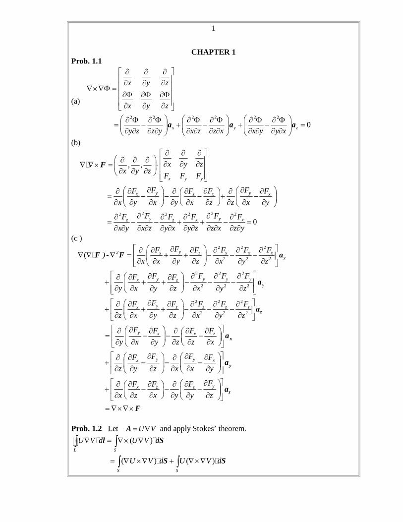
CHAPTER 1 Prob. 1.1

(a)

2 2 2 2 2 2

0x y z

x y z

x y z

y z z y x z z x x y y x

a a a

(b)

2 22 22 2

, ,

0

x y y

y yx x xz

y yx xz z

x y zx y z F F F

F FF F FFx y x y x z z x y

F FF FF Fx y x z y x y z z x z y

� F

(c )

2 2 2

2 2 2

2 2 2

2 2 2

2 2 2

2 2 2

( y2 x x x xzx

y y y yx z

yx z z z z

y

FF F F FF) - x x y z x y z

F F F FF Fy x y z x y z

FF F F F Fz x y z x y z

Fy x

�

y

z

F F a

a

a

x x z

y yx x

yx z z

F F Fy z z x

F FF Fz y z x x y

FF F Fx z x y y z

x

y

z

a

a

a

F

Prob. 1.2 Let U V A and apply Stokes’ theorem.

( )

( ) ( )L S

S S

U V d U V d

U V d U V d

� �

� �

� l S

S S

2

Since 0,V ( )

L S

U V d U V d � �� l S

Similarly, we can show that ( ) ( )

L S S

V U d V U d U V d � � �� l S = - S

Thus,

L L

U V d V U d � �� �l l

as required. Prob. 1.3 Using divergence theorem, ( ) ( )

S v

U V d U V dv � �S

But ( ) , where = VU U U � � �A A A A

2

( ) ( )

( )S v

v

U V d U V V U dv

U V U V dv

� � �

�

S

Prob. 1.4 If 0 ,vJ = then Maxwell’s equations become

0 (1)0 (2)

(3)

(4)

t

t

�

�

BD

BE

DH

Since 0 � A for any vector field A,

0

0

t

t

��

��

BE

DH

Showing that (1) and (2) are incorporated in (3) and (4). Thus Maxwell’s equations can be reduced to curl equations (3) and (4). Prob. 1.5 If 0 ,v J

3

0v

t

t

�

�

EH

HE

EH J

2

2t t t

J EE H

22

2 2

1( )t c t

�J EE E

22

2 2

1 ( / )vc t t

E JE

Similarly,

t

H J E

2

22( ) HH H J

t

�

or

2

22 2

1c t

HH J

It is assumed that the medium is free space so that the medium is homogeneous and 1 .u c

Prob. 1.6 (a)

t

t

DH J

HE

( ) ( ) ( )t t t t

HH J D J E J

2

2t

HH J

(b)2

2( ) ( )t t t t t

D J EE H J

2

2t t

E JE

4

Prob. 1.7

t

HE (1)

t

DH J (2)

Dotting both sides of (2) with E gives

(t

� � �

DE H) E J E (3)

But for any arbitrary vectors A and B, ( ) ( ) ( ) � � �A B B A A B Applying this to the left-hand side of (3) by letting A H and B E , we get

1( ) ( ) ( )2 t

� � � �H E H E E J D E (4)

From (1), 1( ) ( ) ( )2t t

� � �

BH E H B H

Substituting this into (4) gives

1 1( ) ( ) ( )2 2t t

� � � �B H E H J E D E

Rearranging terms and then taking the volume integral of both sides,

1( )2v v v

dv dv dvt

� � � �E H E D H B J E

Using the divergence theorem, we get

( )v

Wd dvt

� �� E H S J E

Or

( )S v

W d dvt

� �� E H S E J

as required. Prob. 1.8

0, 0 � �E H

0

10 sin( ) 20 cos( )

y xx y

x y

x y

E Ex y zdz dzE E

k t kz k t kz

E a a

a a

5

1

10cos( ) 20sin( )

o

x yo

t

k t kz t kz a

H E

a

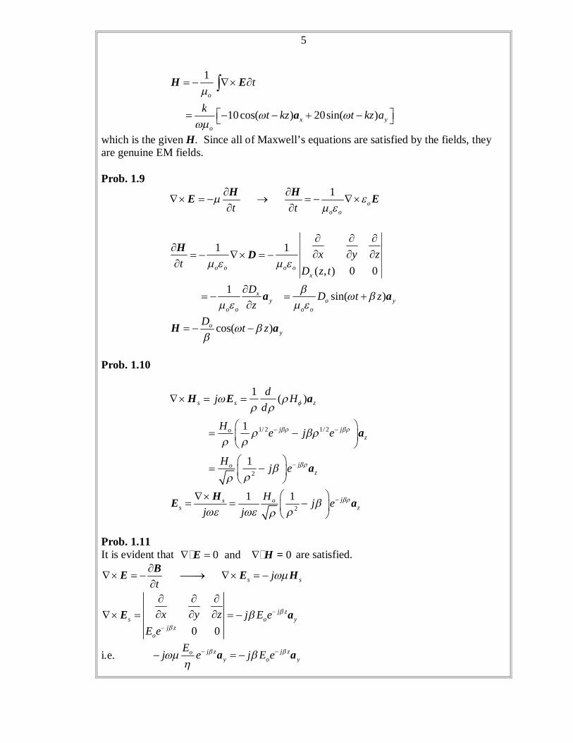
which is the given H. Since all of Maxwell’s equations are satisfied by the fields, they are genuine EM fields. Prob. 1.9

1o

o ot t

H HE E

1 1

( , ) 0 01 sin( )

o o o ox

xy o y

o o o o

x y zt D z t

D D t zz

H D

a a

cos( )oy

D t z

H a

Prob. 1.10

1/ 2 1/ 2

2

1 ( )

1

1

s s z

j joz

joz

dj Hd

H e j e

H j e

H E a

a

a

2

1 1 js os z

H j ej j

HE a

Prob. 1.11 It is evident that 0 and 0 � �E H = are satisfied.

s sjt

BE E H

0 0

j zs o y

j zo

x y z j E eE e

E a

i.e. j z j zoy o y

Ej e j E e

a a

6

(1)

( ) sjt

sDH J H E

0 0

j zos x

j zo

x y z j E eE e

H a

( ) j z j zoo x x

j Ej E e e

a a

( )j j (2) From (1) and (2),

2( ) jj jj

Thus,

,jj

Prob. 1.12 The surface current density is ( ,0, )n n x zH H K a H a At x = 0, , (0, , , )n x z yH y z t a a K a i.e. cos( )o yH t z K a At x = a, n x a a ( , , , ) cos( )cos( )z y o yH a y z t H t z a K a i.e. cos( )o yH t z K a At y =0, n ya a

( ,0, , ) ( ,0, , )

cos( / ) cos( ) sin( / ) sin( )

z x x z

o x o z

H x z t H x z taH x a t z H x a t z

K a a

a a

At y =b, n y a a ( ,0, ) ( , , , ) ( , , , )

cos( / )cos( ) sin( / )sin( )

y x z x z x x

o x o z

H H H x b z t H x b z taH x a t z H x a t z

K a a a

a a

7

Prob. 1.13

(a) 2

22o o t

EE

For E, 2

2 22 cos( ) [ sin( ) cos( )x x xt z t z t z

z z

E a a a

2

2 cos( )o o o o xt zt

E a

Thus, 2 2

o o o o (b)

o dtt

HE H E

sin( )cos( ) 0 0

yx y z t zt z

E a

sin( ) cos( )oo y yt z dt t z

H a a

Prob. 1.14

s sjt t

D EH H E

2

1 1(2sin cos )sin 4

sin 1 14

-j rs r

-j r -j r

IL j er r rIL j j e e

r r r

H a

a

22 2 2

1 12cos sin4

-j rs r

IL j jerj r r r r

E a a

Prob. 1.15

( ) ( ) ( ) ( )

20( )2 2

5

y yx x

x y x y x y x y

jk y jk yjk x jk x

s

j k x k y j k x k y j k x k y j k x k y

e ee eEj j

j e e e e

which consists of four plane waves.

s o sj E H

8

Or

0 0 ( , )

20 sin( )sin( ) cos( )cos( )

s so o

sz

sz szx y

o

y x y x x x y yo

j j x y zE x y

E Ejy x

k k x k y k k x k y

H E

a a

a a

Prob. 1.16 (a) Re( ) sin cos cos( )j t

sI I e x y t z

(b) 2 90 4Re(20 10 )oj x j j t j x j tV e e e e e

2 90 4 2 420 10 20 10oj x j j x j x j x

sV e e e j e e Prob. 1.17 (a) Re( ) cos( 2 ) sin( 2 )j t

s x ye t z t z A A a a (b) Re( ) 10sin sin 5cos( 12 45 )j t o

s x ze x t t z B B a a (c) 3Re( ) 2cos 2 sin( 3 ) cos( 4 )j t x

sC C e x t x e t x Prob. 1.18 Assuming the time factor j te , equation

2

22t t

E JE

becomes 2 2

s s sj E E E or

2 ( ) 0s sj j E E For conducting medium, � so that

2 0s sj E E Prob. 1.19 Let Re( ), Re( ),j t j t

s se V V e A A etc

9

2

22

s

s

jt

t

A A

A A

Similarly,

22

2 sV Vt

Substituting these into eqs. (1.42) and (1.43), we obtain

2 2

2 2

vss s

s s s

V V

A A J

But 2 2k . Thus, 2 2

2 2

vss s

s s s

V k V

k

A A J

Prob. 1.20

(a) a = 1, b = 2, c = 0, b2 – 4ac = -16

Hence, it is elliptic. (b) 2 21, 0, 1,a y b c x 2 2 24 4( 1)( 1) 0b ac x y Hence it is elliptic. (c ) 21, 2cos , (3 sin )a b x c x 2 2 24 4cos 12 4sin 16 0b ac x x Hence it is hyperbolic. (d) 2 2, 2 , ,a x b xy c y 2 2 2 2 24 4 4 0b ac x y x y Hence it is parabolic. Prob. 1.21 (a) 2, 0, 0, 4 0; i.e. it is parabolic.a b c b ac (b) 21, 0, 0, 4 4; i.e. it is elliptic.a b c b ac

(c) 22 2

2 2 0x y

21, 0, 1, 4 4; i.e. it is elliptic.a b c b ac

10

CHAPTER 2 Prob. 2.1 Let ( , ) ( ) ( ).x y X x Y yΦ = '' ' ' '' ' ' 0aX Y bX Y cXY dX Y eXY fXY+ + + + + = Dividing through by XY,

1 1 ' '( '' ') ( '' ') 0bX YaX dX cY eY fX Y XY

+ + + + + =

The PDE is separable if and only if a and d are functions of x only; c and e are functions of y only; b = 0; and f is a sum of a function of x only and a function of y only, i.e. if

1 2( ) ( ) ( ) ( ) [ ( ) ( )] 0xx yy x ya x c y d x c y f x f yΦ + Φ + Φ + Φ + + Φ = Prob. 2.2 (a) Consider the problem as shown below.

This is similar to Example 2.1 with 1 3 2 40, ,o oV V V V V V= = = = − . Hence

odd odd

4 4sinh ( / ) sin( / ) sinh [ ( ) / ]sin( / )( , )sinh( / ) sinh( / )

o o

n n

V Vn x b n y b n a x b n y bV x yn n a b n n a bπ π π π

π π π π

∞ ∞

= =

−= −∑ ∑

But sinh sinh 2cosh sinh2 2

A B A BA B + −− =

odd

4 sin( / )( , ) 2cosh sinh [ ( / 2) / ]sinh( / ) 2

o

n

V n y b n aV x y n x a bn n a b b

π π ππ π

∞

=

= −∑

We now transform coordinates: / 2, / 2x X a y Y b= + = +

x

Vo -Vo

0 a

b y 0

11

odd

sin ( / 2)4 n X( , ) 2cosh sinh

2 b2 sinh cosh2 2

o

n

n Y bV n abV x y

n a n a bnb b

ππ π

π ππ

∞

=

⎛ ⎞+⎜ ⎟⎝ ⎠=⎛ ⎞ ⎛ ⎞⎜ ⎟ ⎜ ⎟⎝ ⎠ ⎝ ⎠

∑

But

sin sin cos( / 2) sin( / 2)cos

2

( 1) cos , oddn

n Y n n Y n Yn nb b b

n Y nb

π π π ππ π

π

⎛ ⎞ ⎛ ⎞ ⎛ ⎞+ = +⎜ ⎟ ⎜ ⎟ ⎜ ⎟⎝ ⎠ ⎝ ⎠ ⎝ ⎠

⎛ ⎞= − =⎜ ⎟⎝ ⎠

odd

( 1) sinh cos( / )4( , )

sinh2

n

o

n

n x n y bV bV x y

n anb

π π

ππ

∞

=

⎛ ⎞− ⎜ ⎟⎝ ⎠=

⎛ ⎞⎜ ⎟⎝ ⎠

∑

(b) Let V(x,y) = X(x)Y(y), / /

1 2( ) sin , ( ) n x b n x bn n

n yY x X x A e A eb

π ππ −= = +

A2 = 0 since X(x) = 0 as x →∞ /( , ) sin( / ) n x b

nV x y a n y b e ππ −=∑

(0, ) sin( / )o nV y V a n y bπ= =∑

o0

0, even2 sin( / ) 4V , odd

b

n o

na V n y b dx

b nn

ππ

=⎧⎪= = ⎨

=⎪⎩∫

/

odd

4 1( , ) sin( / ) n x bo

n

VV x y n y b en

πππ

∞−

=

= ∑

y

x

Y

X

12

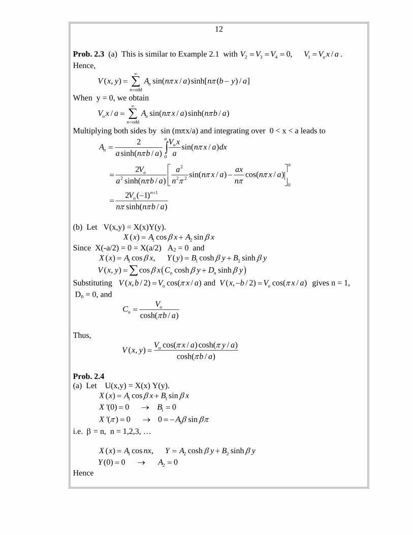
Prob. 2.3 (a) This is similar to Example 2.1 with 2 3 4 10, /oV V V V V x a= = = = . Hence,

odd( , ) sin( / )sinh[ ( ) / ]n

nV x y A n x a n b y aπ π

∞

=

= −∑

When y = 0, we obtain

odd

/ sin( / )sinh( / )o nn

V x a A n x a n b aπ π∞

=

= ∑

Multiplying both sides by sin (mπx/a) and integrating over 0 < x < a leads to

0

2

2 2 20

1

2 sin( / )sinh( / )

2 sin( / ) cos( / )sinh( / )

2 ( 1)sinh( / )

ao

n

a

o

no

V xA n x a dxa n b a a

V a axn x a n x aa n b a n n

Vn n b a

ππ

π ππ π π

π π

+

=

⎡ ⎤= −⎢ ⎥

⎣ ⎦−

=

∫

(b) Let V(x,y) = X(x)Y(y). 1 2( ) cos sinX x A x A xβ β= + Since X(-a/2) = 0 = X(a/2) A2 = 0 and

1 1 2( ) cos , ( ) cosh sinhX x A x Y y B y B yβ β β= = + ( )( , ) cos cosh sinhn nV x y x C y D yβ β β= +∑

Substituting ( , / 2) cos( / ) and ( , / 2) cos( / )o oV x b V x a V x b V x aπ π= − = gives n = 1, Dn = 0, and

cosh( / )

on

VCb aπ

=

Thus,

cos( / ) cosh( / )( , )cosh( / )

oV x a y aV x yb a

π ππ

=

Prob. 2.4 (a) Let U(x,y) = X(x) Y(y). 1 1( ) cos sinX x A x B xβ β= +

1

1

'(0) 0 0'( ) 0 0 sin

X BX Aπ β βπ

= → == → = −

i.e. β = n, n = 1,2,3, … 1 2 2( ) cos , cosh sinhX x A nx Y A y B yβ β= = + 2(0) 0 0Y A= → = Hence

13

01 0

( , ) cos sinh cos sinhn nn n

U x y C C nx ny C nx ny∞ ∞

= =

= + =∑ ∑

0( , ) cos sinhn

nU x x C nx nπ π

∞

=

= =∑

Multiplying both sides by cos mx and integrating over 0< x < π yields / 2oC π= and

2

0, even4 , odd

sinhn

nC

nn nπ π

=⎧⎪= ⎨

=⎪⎩

2odd

4 cos sinh( , )2 sinhn

nx nyU x yn n

ππ π

∞

=

= − ∑

(b) First, transform the equation by letting U(x,t) = x + u(x,t)

where t xxu ku=

Subject to u(0,t) = 0 = u(1,t), u(x,0) = -x If u(x,t) = X(x)T(t),

1 2( ) cos sinX x A x A xβ β= +

1(0) 0 0(1) 0 0 sin

X AX β

= → == → =

i.e. β = nπ.

2 2

2( ) sin , kn tX x A n x T Be ππ −= =

2 2

1( , ) sin kn t

nn

u x t C n xe ππ∞

−

=

=∑

1( ,0) sinn

nu x x C n xπ

∞

=

= − =∑

1

0

2( 1)2 sinn

nC x n xdxn

ππ−

= − =∫

2 2

1

2 ( 1)( , ) ( , ) sinn

kn t

nU x t x u x t x n xe

nππ

π

∞−

=

−= + = + ∑

(c ) Let u(x,t) = X(x)T(t). From the boundary conditions, ( ) cos sinX x A x B xβ β= +

(0) 0 0(1) 0 0 sin

X AX β

= → == → =

or β = nπ. 3 4sin , sin cosX A n x T A n at A n atπ π π= = + 4(0) 0 0T A= → =

14

1

( , ) sin sinnn

u x t C n x n atπ π∞

=

=∑

1( ,0) sint n

nu x x n aC n xπ π

∞

=

= =∑

Multiplying both sides by sin mπx and integrating over 0 < x < 1 yields

2

2cos( )n

n aCn a

ππ

= −

2 2 21

2 cos( , ) sin sinn

n au x t n x n ata n

π π ππ

∞

=

= − ∑

Prob. 2.5 (a) Let ( , ) ( ) ( )R Fρ φ ρ φΦ = . From the text, eq. (2.72) onward, 1 2( ) cos( ) sin( )F C Cφ λφ λφ= +

1 0 since ( ,0) ( , )C ρ ρ π= Φ = Φ . Also, n = 1,2,3,…

( ) sin

( )n n

n nn n n

F C nR a b

φ φ

φ ρ ρ−

=

= +

As 0, ( , )ρ ρ φ→ Φ must be finite, i.e. an = 0.

1

sin( , ) n nn

nA φρ φρ

∞

=

Φ =∑

1

(1, ) sin sinnn

A nφ φ φ∞

=

Φ = =∑

which implies that 1 1, 0 if 1nA A n= = ≠ . Thus sin( , ) φρ φρ

Φ =

(b) From the boundary conditions, Φ does not depend on φ, i.e. m= 0 in F’’ + m2F = 0. From eq. (2.89) in the text,

1 2( ) sin cosZ z C z C zμ μ= + If Z(0) = 0 = Z(L), then 2 0 and or /C L n n Lμ π μ π= = = . Also, 2 2 2'' ' 0R R Rρ ρ μ ρ+ − = 2 2 2 2'' ' ( 0) 0R R j Rρ ρ μ ρ+ + − = The solution to this is 0 0( ) ( ) ( )n nR A I B Kρ ρμ ρμ= + Bn = 0 since K0 is infinite at ρ = 0. Thus

01

( , ) ( / ) sin( / )nn

z A I n L n z Lρ πρ π∞

=

Φ =∑

To obtain An, we apply the boundary condition Φ(a,z) = 1, multiply both sides by sin mz/L, and integrate over 0 < x < L. We get

15

0, even4 , odd

( / )n

o

nA

nn I n a Lπ π

=⎧⎪= ⎨ =⎪⎩

0

1,3,5 0

( / )4 sin( / )( , )( / )n

I n L n z LI n a L n

πρ πρ φπ π

∞

=

Φ = ∑

(c ) Let ( , , ) ( ) ( ) ( )t R F T tρ φ ρ φΦ = . Separation of variables leads to

22' 0 ( ) k tT kT T t e μμ −+ = → =

From eq. (2.88) in the text, ( ) cos sinn n nF a n b nφ φ φ= + Since ( , ,0) cos , 0nbρ φ ρ φΦ = = and ( ) cosn nF a nφ φ= Finally, 2 2 2 2'' ' ( ) 0R R n Rρ ρ μ ρ+ + − = with solution 1 2( ) ( ) ( )n nR c J c Yρ ρμ ρμ= + c2 = 0 since R must be finite at ρ = 0. Hence

2

( , , ) ( ) cos k tn n

nt A J n e μ

μμ

ρ φ ρμ φ −Φ =∑∑

But Φ(a,φ,t) = 0 implies that ( ) 0 ( )n n mJ a J Xμ = = where Xm are the roots of Jn and µ = Xm/a . Also, 2( , ,0) cos 2 ( )cosn n

nA J nμ

μ

ρ φ ρ φ ρμ φΦ = =∑∑

It is evident that n = 2 and that 2

2 2 ( )A Jμμ

ρ ρμ=∑

which is the Fourier-Bessel expansion of ρ2. From Table 2.1, property (h),

22 22 2

3 30

2 2( )[ ( )] ( )

a

m m

A J da J a X J Xμ ρ ρμ ρ

μ= =∫

Thus

2 22

1 3

( / )( , , ) 2 cos 2 exp( / )( )

mm

m m m

J X at X kt aX J Xρρ φ φ

∞

=

Φ = −∑

where 2 ( ) 0mJ X = . Prob. 2.6

2

2

U Ux t

∂ ∂=

∂ ∂