solution techniques for large eigenvalue problems in
TRANSCRIPT
'±~ctA ..... Lt/'. 'J.-
UILU-ENG-79-2006
~.3 ~ , CIVIL ENGINEERING STUDIES
STRUCTURAL RESEARCH SERIES NO. 462
SOLUTION TECHNIQUES FOR LARGE EIGENVALUE PROBLEMS IN STRUCTURAL DYNAMICS
II Metz Reference Room
Civil Engineering Department BI06 C.E. Building
University of Illinois Urbana" Illinois. 6180li
By I.-W. LEE
A. R. ROBINSON
A Technical Report of Research Sponsored by
THE OFFICE OF NAVAL RESEARCH DEPARTMENT OF THE NAVY
Contract No. N00014-75-C-0164 Project No. NR 064-183
Reproduction in whole or in part is permitted for any purpose of the United States Government.
Approved for Public Release: Distribution Unlimited
UNIVERSITY OF ILLINOIS
at URBANA-CHAMPAIGN
URBANA, ILLINOIS
JUNE 1979


50272-101
REPORT DOCUMENTATION 1_1./;REPORT NO.
PAGE TTTT,TT ENG-79-2006
2. 3. Recipient'. Acce •• lon No.
4. Title and Subtitle
Solution Techniques for Large Eigenvalue Problems in Structural Dynamics
5. Repo·rt Date
June 1979
---------------- ----------_._--------..-------7. Author(s)
In-Won Lee and Arthur R. Robinson 9_ Performing Organization Name and Address
Department of Civil Engineering University of Illinois at Urbana-Champaign Newmark Civil Engineering Laboratory 208 N. Romine Street TT."..1-..... T1...,; ...... ,....;c h1Q(\1
12. SPo~~;ri'j;g' Organiz;ti~~ "N';me ~';d Address
Material Science Division Structural Mechanics Program (code 474) Office of Naval Research (800 Quincy Street) Arlington, Virginia 22217
15. Supplementary Notes
--------------------_. ------------16. Abstract (limit: 200 words)
8. Performing Organization Rept. No.
SRS No. 462 10. Project/Task/Work Unit No.
NR 064-183 11. Contract(C) or Grant(G) No.
(C) N00014-75-C-0164
(G)
13. Type of Report & Period Covered
Technical Report r---------------------------~
14.
--- --------------------1
This study treats the determination of eigenvalues and eigenvectors of large algebraic systems. The methods developed are applicable to finding the natural frequencies and modes of vibration of _large structural systems.
For distinct eigenvalues the method is an application of the modified NewtonRaphson method that turns out to be more efficient than the standard competing
schemes.
For close or multiple eigenvalues, the modified Newton-Raphson method is generalizec to form a new process. The entire set of close eigenvalues and their eigenvectors are found at the same time in a two-step procedure. The subspace of the approximate eigenvectors is first projected onto the subspace of the true eigenvectors. If the eigenvalues are multiple, the results of the first stage indicate this fact and the process terminates. If they are merely close, a single rotation in the newly found space solves a small eigenvalue problem and provides the final results for the close set. The procedure for subspace projection can be expressed as a simple extremum proble~ that generalizes the known extremum property of eigenvectors.
Computational effort and convergence are studied in three example problems. The method turns Out to be more efficient than subspace iteration.
-----------------------------------------------------------------~ 17. Document Analysi5 a. Descriptof"l
Eigenvalues Eigenvectors Numerical Analysis Dynamic Structural Analysis b. Identifiers/Open-Ended Terms
c. COSAT! Fie!d/Group
18. Avaiiability Statement
Approved for public release: Distribution unlimited
21. No. of Pages
118 19. Security Class (This Report)
Unclassified ~--------------~----------------
20. Security Class (This Page) 22. Price
Unclassified See ANSI-Z39.1S, See Instructions on Reverse OPTIONAL FORM 272 (4-77)
(Formerly NTIS-35) Department of Commerce


SOLUTION TECHNIQUES FOR LARGE EIGENVALUE
PROBLEMS IN STRUCTURAL DYNAMICS
by
I.-W. Lee
A. R. Robinson
A Technical Report of
Research Sponsored by
THE OFFICE OF NAVAL RESEARCH DEPARTMENT OF THE NAVY
Contract No. N00014-75-C-0164
Project No. NR 064-183
Reproduction in while or in part is permitted for any purpose of the United States Government.
Approved for Public Release: Distribution Unlimited
University of Illinois at Urbana-Champaign Urbana, Illinois
June 1979


iii
ACKNOWLEDGMENT
This report was prepared as a doctoral dissertation by
Mr. In-Won Lee and was submitted to the Graduate College of the
University of Illinois at Urbana-Champaign in partial fulfillment of
the requirements for the degree of Doctor of Philosophy in Civil
Engineering. The work was done under the supervision of
Dr. Arthur R. Robinson, Professor of Civil Engineering.
The investigation was conducted as part of a research program
supported by the Office of Naval Research under Contract N00014-75-C-
0164, "Numerical and Approximate Methods of Stress Analysis. II
The authors wish to thank Dr. Leonard Lopez, Professor of
Civil Engineering, for his assistance.
The numerical results were obtained with the use of the
CYBER-75 computer system of the Office of Computer Services of the
University of Illinois at Urbana-Champaign.

iv
TABLE OF CONTENTS
Page
1 . INTRODUCTION......
2.
1 . 1 Genera 1 . . . . . . 1.2 Object and Scope ..... 1.3 Review of Solution Methods. 1 . 4 No ta t ion . . . . . . . . . . . . . . .
DISTINCT ROOTS ..
2. 1 2.2 2.3 2.4 2.5
General . . . . . . . The Iterative Scheme . . . . . . . . . Convergence Rate and Operation Count . Errors in Approximate Eigenso1utions . Treatment of Missed Eigenso1utions
1 2 3 6
10
10 10 14 17 19
3. CLOSE OR MULTIPLE ROOTS ........ . 21
3.1 General .......................... 21 3.2 Theoretical Background. . . . . . . . . . . . . . . . . 22 3 . 3 Th e I t era t i ve S chern e . . . . . . . . . 25 3.4 Treatment of Close Roots . . . . . . . 30 3.5 Convergence Rate and Operation Count 31
4. APPROXIMATE STARTING EIGENSOLUTION . 34
5.
4. 1 Genera 1 . . . . . . . . . . . . . . 34 4.2 Subspace Iteration Method . . . . . . 35
4.2.1 The Iterative Scheme. . . . . 35 4.2.2 Starting Vectors. . . . . . . . 37 4.2.3 Convergence Rate, Operation Count, and
Estimation of Errors. . . . . . . . 38 4.3 Starting Solution for the Proposed Method 41
NUHER I CAL RESULTS AND COMPARISONS . . . 43
5. 1 Genera 1 . . . . . . . . . • . . . • . • . . . . . . . . •. 43 5.2 Plane Frame. . . . . . . . . . . . . . . . . . . . . . .. 44 5.3 Arch . . . . . . . . . . . . . . . . . . . . . . . . . . . . 45 5.4 Plate Bending. . . . . . . . . . . . . . . . . . . . . .. 46 5.5 Comparison between the Theoretical Convergence Rates and
Numerical Results . . . . . . . . . . . . . . . . . . . .. 47
6. SUM~ARY AND CONCLUSIONS ...... . 49
49 50 51
6. 1 6.2 6.3
Summary of the Proposed Method Conclusions .. . ... Recommendations for Further Study . . . . . . . . . . . . .

v
Page
LIST OF REFERENCES . . . . . . . . . . . . . . . . . . . . . . . . . 52
APPENDIX A. NONSINGULARITY OF THE COEFFICIENT MATRICES OF
THE BASIC EQUATIONS . . . . . . . . . . . . . 57
B. CONVERGENCE ANALYSIS . . . . . . . . . . . . . . . . . . . . 61
B.1 Case of a Di·stinct RDot B.2 Case of a Multiple Root
C. THE BASIC THEOREMS ON THE CONSTRAINED
61 67
STATIONARY-VALUE PROBLEM . . . . . . . . . . . . . . . . . . 77

vi
LIST OF TABLES
Table Page
1. NUMBER OF OPERATIONS FOR EIGENSOLUTIONS ....... . . . 86
2. EIGENVALUES OF THE PLANE FRAME PROBLEM (DISTINCT ROOTS) ..... 90
3. EIGENVALUES OF THE CIRCULAR ARCH PROBLEM (DISTINCT ROOTS) .... 92
4. EIGENVALUES OF THE SQUARE PLATE PROBLEM (DOUBLE ROOTS) . . . 94
5. EIGENVALUES OF THE RECTANGULAR PLATE PROBLEM (CLOSE ROOTS) . 95
6. COMPARISON OF THE TOTAL NUMBER OF OPERATIONS 96
7. COMPARISON BETWEEN THE THEORETICAL CONVERGENCE RATES FOR EIGENVECTORS AND THE NUMERICAL RESULTS - FRAME PROBLEM (DISTINCT ROOTS) . . . . . . . . . . . . . . . . . . . . . . . . 97
8. COMPARISON BETWEEN THE THEORETICAL CONVERGENCE RATES FOR EIGENVECTORS AND THE NUMERICAL RESULTS - SQUARE PLATE PROBLEM (DOUBLE ROOTS) . . . . . . . . . . . . . . . . . . . . . 98
9. NUMERICAL CONVERGENCE RATES FOR EIGENVECTORS -RECTANGULAR PLATE PROBLEM (CLOSE ROOTS) . . . . . . . . . . . . . 99
.t:' nee Room Metz Re~ere t . neering Departmen
Civ~l Engi .l~·ng C E BUl ell Bl06 .~ . f Illinoia
Univers~vY ~ 's 6180] Urbana" Illl.nol. - -


vii
LIST OF FIGURES
Figure Page
1. ESTIMATION OF ERRORS IN APPROXIMATE EIGENVECTORS. 100
2. TEN-STORY, TEN-BAY PLANE FRAME. . . . . . . . . . 101


1
1. INTRODUCTION
1.1 General
Various engineering problems can be reduced to the solution of matrix
eigenvalue problems. Typical examples in the field of structural engineering
are the problem of determination of natural frequencies and the corresponding
normal modes in a dynamic analysis and the problem of finding buckling loads
in a stability analysis of structures. Since the advent of the digital com
puter, the complexity of structures which can be treated and the order of
the corresponding eigenvalue problems have been greatly increased. Hence,
the development of solution techniques for such problems has attracted much
attention.
For the dynamic analysis of a linear discrete structural system by
superposition of modes, we must first solve the problem of free vibration
of the system. The free vibration analysis of the linear system without
damping reduces to the solution of the linear eigenvalue problem
Ax = A Sx (1.1)
in which A and B are stiffness and mass matrices of order n, the number of
degrees of freedom of the structural system. A column vector x is an
eigenvector (or normal mode), and the scalar A the corresponding eigenvalue
(or the square of a natural frequency).
Th2 matrices A and B are real and symmetric, and are usually banded and
sparse. If a consistent mass matrix is used, the matrices A and B have the

2
same bandwidth [4,5J. If a lumped mass model of the system is used, B will
be diagonal. The matrix B is positive definite, but the matrix A may be
semidefinite. There are n sets of solutions of Eq. (1.1), that is, n eigen
values and their corresponding eigenvectors.
Frequently, in practical eigenvalue problems, the order of A and B is
so high that it is impractical or very expensive to obtain the complete
eigensolution. On the other hand, to carry out a reasonably accurate
dynamic analysis of the structure, it is possible to consider only a partial
eigensolution. The partial solution of interest may consist of only few
lowest eigenvalues and their eigenvectors, or eigenvalues in the vicinity
of a given frequency and the corresponding eigenvectors. The method
described in this study is aimed at effective solution of this type of
problem rather than at a complete eigensolution.
1.2 Object and Scope
The object of this study is to present an iterative method which is
efficient and numerically stable for the accurate computation of limited
number of eigenvalues and the corresponding eigenvectors of linear eigenvalue
problems of large order.
The method developed remedies the major drawbacks of the inverse iter
ation method with spectral shifting [13]: numerical instability due to
shifting and slow convergence when eigenvalues are equal or close in magni
tude. The proposed method converges rapidly and is numerically stable for any
number of multiple or close eigenvalues and the corresponding eigenvectors.

3
The procedure for distinct eigenvalues is treated in Chapter 2, and a
modified procedure for multiple or close eigenvalues in Chapter 3. Selection
of initial approximate eigenvalues and eigenvectors by the subspace iteration
method is described in Chapter 4. To show the efficiency of the proposed
method, three sample problems are solved: vibration of a plane frame, of
a plate in bending, and of an arch. Comparisons are made in Chapter 5 with
a method which is generally regarded as very efficient, the subspace
iteration method.
1.3 Review of Solution Methods
Numerous techniques for the solution of eigenvalue problems have been
developed. These techniques can be divided into two classes - techniques
for approximate solution and techniques for "exact ll solution.
The approximate solution techniques include well-known static conden
sation [2,3,24,25,27,42J, dynamic condensation [34J, Rayleigh-Ritz analysis
[9,13,31,48J, component mode analysis and related methods summarized by
Uhrig [50J. These methods are essentially techniques for reducing the size
of a system of equations. The reduction of a system of equations eventually
leads to a loss in accuracy of a solution. However, the advantage of
lessened computational effort for a solution sometimes may compensate for
the loss in accuracy. Moreover, an approximate solution found by these methods
may serve as the starting solution for the exact methods, which will be
discussed next.
The exact methods are designed for the accurate computation of some
or all the eigenvalues and corresponding eigenvectors. These methods consist

4
of vector iteration methods, transformation methods, the method based on
the Sturm-sequence property, polynomial iteration method, and minimization
methods. These methods are well described in Ref. 51. The methods differ
in the choice of which mathematical properties of an eigenvalue problem are
used. The vector iteration methods such as the classical vector iteration
(power method) and simultaneous vector iteration deal with the form of
equations Ax = A Sx. The transformation methods (LR, QR, Jacobi, Givens,
and Householder methods) are based on the mathematical property that the
eigenvalues of a system are invariant under similarity transformations. In
the polynomial iteration method, the roots of det (A - AS ) = 0 are found,
and minimization methods are based on the stationary property of the
Rayleigh quotient [43J.
In vector iteration methods and minimization methods, both the eigen
values and corresponding eigenvectors are found simultaneously, but in
other exact methods, only eigenvalues are computed or the computed eigen
vectors are, in general, not suitable for use in the final solutions. In
such methods, another method such as the vector iteration method with a
shift may be used for finding the eigenvector corresponding to a computed
eigenvalue.
For a limited number of eigenvalues and corresponding eigenvectors df
an eigenvalue problem of large order which we are concerned with in this
study, the above methods have been modified or combined to take advantage
of the useful characteristics of several of the methods. First, the
determinant search method [7,9,22,23J combines the methods based on the Sturm
sequence property, polynomial iteration, and inverse iteration. In this

5
method, eigenvalues in a specified range are approximately isolated by using
the bisection method and the Sturm-sequence property and then located
accurately by the polynomial iteration method. The corresponding eigen
vectors are computed by inverse iteration with a shift. By this method,
eigenvalues in any range and corresponding eigenvectors can be found.
However, it has the disadvantage that the matrix is factorized in each iter
ation to locate the eigenvalues of interest.
Another method for the solution of large eigenvalue problems is the
so-called subspace iteration method [6,15,32,39,47J, which is a combination
of the simultaneous iteration method and a Rayleigh-Ritz analysis. In this
method, several independent vectors are improved by vector inverse iteration,
and the best approximation to the eigenvectors are found in the subspace of
the iteration vectors by a Rayleigh-Ritz analysis. In this method, eigen
values at the end of the spectrum and the corresponding eigenvectors converge
very rapi dly. Thi s method wi 11 be d-i scussed further in Chapter 4.
The inverse iteration method with a shift is known to be extremely
efficient for improving approximate eigenvalues and eigenvectors. However,
as mentioned in the previous section, when the shift is very close to a true
eigenvalue, the method exhibits numerical instability, yielding unreliable
answers [13J. In addition, when the eigenvalues of interest are close to
gether, their convergence is very slow. Robinson and Harris [44J developed
an efficient method to overcome the above difficulty for distinct eigenvalues
by augmenting the equations used in the inverse iteration method by a side
equation. While this method extracts eigenvalues and eigenvectors simul
taneously with a very high convergence rate, it has the disadvantage that the

6
algorithm is inefficient for problems with multiple or close eigenvalues.
This method and some improvements on it will be discussed further in the
next chapter.
1.4 Notation
All symbols are defined in the text when they first appear.
With regard to matrices, vectors, elements of matrices or vectors, and
iteration steps, the following conventions are generally used:
(1) Matrices are denoted by uppercase letters, as A, Band X.
(2) A column vector is denoted by a lowercase letter with a
(3)
(4)
(5 )
superior bar and a subscript, as ~.- b. and x .. - J" - J -- --- - J
Elements of a matrix or vector are denoted by a lowercase
1 e t te r with ado u b 1 e sub s c rip t s, a sa. ., b.. and x. . . lJ lJ lJ
Iteration steps are denoted by a superscript, as x(k), x~k) J
(k) and x ... lJ
Increments are denoted by the symbol ~, as ~x~k) and ~X~~). J 1 J
Some symbols are assigned more than one meaning. However, in the context
of their use there are no ambiguities.
- -A, a·, a·· J lJ
*(k) A "
a
B, 6., b .. J lJ
*(k) B
= stiffness matrix, jth column vector of A, element
of A
= projection of A onto the subspace spanned by vectors
= radius of circular arch
. . th 1 t f B 1 t f B = mass matrlx, J co umn vec or 0 ,e emen 0
= projection of B onto the subspace spanned by vectors
in y(k), B*(k) = y(k)T B y(k)

o
0, 0. J
E
-E, e., e .. J JJ
* -* -* E , e., e.· J JJ
h
I
i, j
k
L
m , mb a
7
= expansion matrix of X(k), jth column vector of C(k),
element of C(k), X(k) = XC(k)
= diagonal matrix, see Section 2.2
= plate bending stiffness, De = EH3/12(1-u2)
= matrix for finding close or multiple eigenvalues and
eigenvectors, jth column vector of 0, see Eq. (3.24)
= iteration matrix for Dafter k iterations, jth column
vector of D (k), see Eq. (3.23)
= Young's modulus
= diagonal matrix, jth column vector of E, element of
E, see Eq. (A.7)
* = diagonal matrix, jth column vector of E , element of
E*, E* = _E- l
= thickness of plate
= number indicating rate of convergence of eigenvector,
see Eq. (2. 13)
= moment of inertia of cross-section
= identity matrix of order s
= indices of matrix elements
= superscript indicating number of iterations
= lower triangular matrix
= Lagrangian, see Eq. (3.6)
= average half bandwidth of A, "oF R VI U
= total number of operations required for finding
eigenpairs by the proposed method, by the Robinson-
Harris method, by the subspace-iteration method
n
p
q
- (k) r. J
s
-x, x. , J
X(k),
x .. lJ
-(k) x· , J
y(k), y~k), J
o .. lJ
e~k) J
*
11, A. J
x~~) lJ
y~ ~) lJ
8
= order of A and B
= number of eigenpairs sought
= number of iteration vectors by subspace iteration
method, q = max(2p, p+8)
= residual vector of approximation to jth eigenpair
after k iterations
= number of close and/or multiple eigenpairs sought
= number of iterations needed to find eigenpairs by
proposed method, by Robinson-Harris method, by
subspace iteration method
= matrix of eigenvectors (modal matrix), jth eigen-
vector, element of X
= approximation to X after k iterations, jth column
vector of X(k), element of X(k)
= matrix of iteration vectors improved from X(k) by
simultaneous iteration method, jth column vector of
y(k), element of y(k)
= rotation matrix, approximation to Z after k iterations
= error in A~k) or ~~~) J JJ
= increment operator
= Kronecker delta
= error in x~k) or y~k) J J
= multiple eigenvalue
= diagonal matrix of eigenvalues, jth eigenvalue,
11 = diag(Al' A2' ... , AS)

9
A(k) A(k) = approximation to A, to Aj' after k iterations j
l.l = shift applied in vector iteration method
l.l' • , (k) = element of 0, of D(k) 1-1- •
lJ lJ
P = mass density
= natural circular frequency, A = 2 w w

10
2. DISTINCT ROOTS
2.1 General
In this chapter, a method for finding a simple eigenvalue and the
corresponding eigenvector will be presented. The method developed by
Robinson and Harris [44J is modified here to save overall computational
effort for finding an eigensolution. The Robinson-Harris method is an
application of the Newton-Raphson technique for improving the accuracy of
an approximate eigenvalue and the corresponding approximate eigenvector.
In the proposed method, a modified form of the Newton-Raphson technique is
applied instead of the standard one used in the Robinson-Harris method.
In Section 2.2, the Robinson-Harris method will be discussed first;
then the proposed method will be presented. The convergence rate of the
proposed method and the number of operations per iteration will be given in
Section 2.3. The estimation of error in an approximate solution is found
in Section 2.4. A technique for the examination of the converged solution
to determine whether the eigenvalues and corresponding eigenvectors of
interest have been missed and a method for finding a missed solution will
be presented in Section 2.5.
2.2 The Iterative Scheme
Let us consider the following linear eigenvalue problem
Ax. = A. Bx. J J J
(j = 1, 2, . . . , n) (2.1)

11
where A and B are assumed to be given symmetric matrices of order nand B
is taken to be positive definite. The A. and X. are the jth eigenvalue and J J
the corresponding eigenvector.
Let us assume that an initial approximate solution of Eq. (2.1), A. (0) J
and x.(O), is available. Denote an approximate eigenvalue and the corre-J
sponding eigenvector after k iterations by A/ k) and x/ k) (k = 0, l, ... ).
Then, we have
- (k) Ax. J
where rj(k) is a residual vector.
- (k) r. J
(2.2)
The object is to remove the residual vector in Eq. (2.2). The Newton
Raphson technique is applied for this purpose. Let the (k + l)th approxi
mation be defined by
A • (k+ 1) = J
- (k+l) x. =
J - (k) - (k) x. + !:J.x.
J J (2.3)
where ~A.(k) and ~x.(k) are small unknown incremental changes of A.(k) and J J J
x (k) Sub s tit uti n g A. (k + 1) and XJ. (k + 1) 0 f E q . ( 2 . 3) for A. and X. i n
j . J J J
Eq. (2.1) and discarding a nonlinear term ~A.(kLB~x.(k) as very small J J
compared with the other, linear, terms, We get
- (k) r. J
(2.4)
where r. (k) is the residual vector defined in Eq. (2.2). J

12
Note that in Eq. (2.4), there are n+l scalar unknowns (IlA.(k) and n J
compone~ts of llX.(k)), but only n equations. Hence, it is required for the J
solution of Eq. (2.4) that either the number of unknowns be reduced or one
equation added. Derwidue [16J and Ra11 [41J reduced the number of unknowns . by setting the nth component of the vector lli.(k) or i.(k+l) at a preassigned
J ,J
value - zero or one. In these methods, it may happen that an unfortunate
choice of one component results in failure of the procedure. \
Instead of reducing the number of unknowns, Robinson and Harris [44J
added an extra equation (side condition) to the system of Eq. (2.4), to
arrive at a set of n+l equations in n+l unknowns. This side condition is
T x . ( k) . BllX. ( k) = 0 (2. 5 ) J J
Equation (2.5) means that the incremental value llX.(k) is orthogonal to J
the current approximate eigenvector x.(k) with respect to the matrix B. J
The side condition prevents unlimited change in the xj(k). The resulting
set of simultaneous linear equations may be written in matrix form as·
- (k) - Bx. J
- (k) - (k) llx . r. J J
= (2.6)
llA.(k) 0 J
_ (k) T x. B
J o
where the residual vector r.(k) is given in Eq. (2.2). The coefficient J
matrix for the incremental values is of order n+l and symmetric. Moreover,
it is nonsingular if A. is not multiple [44J. Equation (2.6) may be solved J
for llA.(k) and llX.(k) by Gauss elimination, or by any other suitable J J

13
technique. Note that the submatrix in the coefficient matrix (A - A.(k)B) J
is almost singular when A.(k) is close to A .. However, this does not cause J J
any difficulty in solving Eq. (2.6), since in the elimination process only
the last pivot element, in general, becomes very small. Thus, the inter-
change of columns and rows does not increase significantly the column height
of the factorized matrix. The improved values, A. (k+1) and X. (k+1), are J J
computed from Eq. (2.3). The procedure employing Eqs. (2.3) and (2.6) is
repeated until the errors in the A.(k) and x.(k) are within allowable toler-J J
ances. The method of estimating these errors will be discussed in Sec-
tion 2.4.
The convergence of the above process for an eigenvalue and the corre-
sponding eigenvector has been shown to be better than second order; the
order has been found to be 2.41 [44J. However, the algorithm using Eq. (2.6)
requires a new triangularization in each iteration, since the values of the
elements of the coefficient matrix are changed in each iteration as a result
of changing from Aj(k) to Aj(k+l). The number of operations (multiplications
and divisions) required in such a triangularization is very large.
To avoid the complete elimination procedure in each iteration, the
following equations instead of Eq. (2.6) are used in the proposed method.
A - A. (O)B - (k) - (k) - (k) -Bx. 6X. - r. J J J J
(2.7)
l - T 6A.(k) x . (k) B 0 0
J J

14
where the residual vector r.(k) is defined in Eq. (2.2). Equation (2.7) J
was obtained by introducing Eq. (2.3) into Eq. (2.1) and discarding a small
linear term (A.(k+l) - 1...(0)) BllX.(k). Note that Eq. (2.7) differs from J J J
Eq. (2.6) in such a way that the coefficient matrix in Eq. (2.6) has the
submatrix (A - Aj(k)B), while the coefficient matrix in Eq. (2.7) has
(A - Aj(O)B). The coefficient matrix in Eq. (2.7) is also symmetric, and
non sin g~ 1 a r if' t 1 t' 1 A J 1 S no mu 1 p e. The nonsingularity of the coefficient
matrix will be prove~ in passing, in Appendix A.
From the form of the coefficient matrix, it can be seen that once the
matrix is decomposed into the form LDLT, where L is lower triangular and 0
_is diagonal, only a small number of additional operations is required
for the solution of Eq. (2.7) in the succeeding iterations, since only the
vector Bx. (k) in the matrix is changed in each iteration. The proposed J
method therefore considerably reduces the number of operations required in
each iteration. On the other hand, the method lowers the convergence rate
because of the neglect of the small linear term (A.(k+l) - 1...(0)) (BllX.(k)), J J J
which in turn increases the number of iterations for a solution. However,
the overall co~putational effort for a solution does decrease. It will be
seen in Chapter 5 that the proposed method is actually more efficient than
the Robinson-Harris method.
2.3 Convergence Rate and Operation Count
The efficiency of a numerical method such as the one proposed here can
be estimated given the convergence rate and the number of operations per
iteration required in the process. The convergence analysis, which is given

15
in Appendix B, will be summarized as follows. Let an approximate eigenvector - (k) Xj be expanded in terms of the true eigenvectors xi' i.e.,
n x.(k) = r
J ._-' c .. (k) X.
1 J 1 (2.8)
i=l
h ( k) . ff' . t f th t If YJ' (k) 1'S the error ,. n were c.. 1 sac 0 e 1 c 1 en 0 eve cor x ..
1J ,
A.(k) and e .(k) the error in x.(k), they may be defined as J J J
y.(k) = J
A. - A.(k) J J
A,. J
n ,-. ( (k)2 c. . ) "- .. , 1 J i=l
(2.9)
1/2
(2. 10)
v/here e.(k) is a measure of the angle between the vectors c.(k) and c., and _J(k)T J J
vJhere c. = (c1.(k), c2
.(k), ... , C .(k) and c~ = (0, .. ,0, c .. (k),O, ... ,O). J J J nJ J J J
The geometric interpretation of 8j (k) is illustrated in Fig. 1.
With the above definitions, the errors in A.(k+1) and x.(k+1) may be J J
written as (see Appendix B)
(2.11)

16
e . ( k+ 1) = he. ( k) (2.12) J J
where
h = max m~j A - 1..(0)
m J
< (m = 1, 2, ... n) (2.13)
Equatiops (2.11) and (2.12) show that the convergence character of both
eigenvalues and eigenvectors is linear.
much more rapidly than the eigenvectors.
However, the eigenvalues converge
Note also that the closer A. is J
to another eigenvalue, the larger a is, yielding slow convergence. Hence,
the method is not suitable for finding close eigenvalues and the corre-
sponding eigenvectors.
Another important consideration which should be taken into account in
estimating the efficiency of numerical methods is the number of operations
per iteration. One operation is defined as one multiplication or division,
which almost always is followed by an addition or a subtraction. For the
expression of this number, let rna and mb be the half band-widths of the
matrices A and B, and let n be the order of A and B. Let T be the number p
of iterations needed to find p eigenpairs by the proposed method and T by r
the Robinson-Harris method. Then, the number of operations for p eigenpairs,
N , required by the proposed method is p
-- , ,2 _ ~ ~ +_ ?)\ fi = ~n \ m +.:Sm + Lm '-
p 2 a a b + T n (5m + 2mb + 6)
P a (2.14)

17
and by the Robinson-Harris method, N , is r
Nr = IT n (m2 + 13m + 6 + 12) 2 r a a mb (2.15)
It can be seen that the number of operations per iteration required by the
proposed method is much smaller than for the Robinson-Harris method. The
development of the above expressions is given in Table 1.
2.4 Errors in Approximate Eigensolutions
An important feature of an iterative method such as the proposed method
is some means of estimating the error in a computed solution. This permits
one to terminate the iteration process at the point where a sufficiently
accurate result has been obtained. It is important to have estimates in
terms of numbers available in the calculation, since it is impossible to
compare with the exact values.
The error in A.(k), y.(k), can be estimated as follows: from J J
Eqs. (2.9) and (2.11)
A. = A.(k+l) J J
Substituting Eq. (2.16) for Aj in Eq. (2.9) gives
y.(k) = J
=
A • (k) 1 - ---:J"'---_
Aj
(2. 1 6)
(2. 17 )

18
Since 0 < h « 1 and 0 < y.Ck) « 1, from Eq. (2.17) - J
A • (k) 1 - J
A ( k+1)
(2.18)
The error in x.(k), e.(k), can be approximated by [e.(k) - e.(k+1)] J J J J
since e.(k+1) «s.(k). Furthermore, from Fig. 1, J J
n L(~c .. (k¥
lJ
1/2
i=l (k+ 1) i!: j - s. ::::: _r---__ _
J
T ~x. (k) B~x. (k)
1/2
= J J (2.19) _ (k)T - (k) x· Bx.
J J
Therefore,
T 1/2
s . (k) ~x. (k) B~x. (k)
J J (2.20) - T J - (k) - (k) x· Bx.
J J L

19
The number of operations for the estimation of e.(k) is only about J
n (2mb + 3), which is small compared with the number of operations per iter-
ation (see Section 2.3).
2.5 Treatment of Missed Eigensolutions
Some of the eigenvalues and corresponding eigenvectors of interest may
be missed when the initial approximations are not suitable. In order to
check whether this occurs, the Sturm-sequence property [9,31,39,48,51J may
be applied. The Sturm-sequence property is expressed as follows: if for
an approximate eigenvalue A.(O), (A - A.(O)B) is decomposed into LOLT, J J
where L is a lower triangular matrix and 0 a diagonal one, then the number
of negative elements in 0 equals the number of eigenvalues smaller than
Aj(O). A computed eigenvalue can be checked using the above property with
negligible extra computation, since the decomposition of t~e matrix
(A - A.(O)B) has already been carried out during the procedure for the J
solution of Eq. (2.7).
If some of the eigenvalues of interest are detected to be missing,
finding them consists of three steps: finding approximations to the missed
eigenvalues~ finding approximate eigenvectors corresponding to the missed
eigenvalues, and improving the approximate eigensolutions.
The approximate eigenvalues can be found by the repeated applications
of the Sturm-sequence calculation mentioned above and the method of bisection
[9,31,38,51J, or by the polynomial iteration method [7,8,9,38,51J, in which
the zeros of the characteristics polynomial p(A) = det(A - AB) are found
using variants of Newton's method.
20
In the second step, the approximation to the eigenvectors corresponding
to the missed eigenvalues is found. Frequently, finding the eigenvectors
corresponding to the missed eigenvalues is much more difficult than finding
the missed eigenvalues. However, subspace iterations with a shift [6,32J,
which will be discussed in Chapter 4, or dynamic condensation [34,42,50J
may be used for this purpose.
Finally, the approximate eigenvalues and corresponding approximate
eigenvectors can be improved by the method of Section 2.2 if the eigen
values are not multiple or close, or if they are, by the method of
Chapter 3.

21
3. CLOSE OR MULTIPLE ROOTS
3.1 General
As mentioned earlier, the method presented in Chapter 2 fails or
exhibits slow convergence if it is applied to the solution for multiple or
close eigenvalues and for their corresponding eigenvectors. The failure or
slow convergence of the method is caused by impending singularity of the
coefficient matrix for the unknown incremental values as the successive
approximations approach the true eigenvalue and eigenvector.
The method presented in this chapter overcomes this shortcoming. To
accomplish this, all eigenvectors corresponding to multiple or close eigen
values are found together. As in the method of Chapter 2, this method
yields the eigenvalues and corresponding eigenvectors at the same time.
The essence of the method consists first in finding the subspace
spanned by the eigenvectors corresponding to multiple or close eigenvalues.
The subspace is found using the Newton-Raphson technique in a way suggested
by the Robinson-Harris method [44J. If the eigenvalues of interest are
multiple, any set of independent vectors spanning subspace are the true
eigenvectors, but if the eigenvalues are merely close together, the
vectors must be rotated in the subspace to find the true eigenvectors. The
eigenvalues are obtained as a by-product of the process of finding the sub
space and any subsequent rotation. In this method, any number of close
eigenvalues or an eigenvalue of any multiplicity can be found together with
the corresponding eigenvectors.

22
The theoretical background of the method is presented in S~ction 3.2
The iterative scheme for finding the subspace of the eigenvectors corre
sponding to multiple or close eigenvalues is given in Section 3.3. The
additional treatment required for close eigenvalues and corresponding
eigenvectors is the subject of Section 3.4. The convergence rate and the
number of operations per iteration are given in Section 3.5.
3.2 Theoretical Background
Let us consider the system treated in Chapter 2, i.e.,
Ax. = A. BX. 1 1 1
(i = 1, 2, .. , , n) (3.1)
where A and B are symmetric matrices of order n, and B is positive definite.
-The ei genvectors, and the Ai eigenvalues in the order A1< A2 < , ... , <A . x. are 1 - - - n
Let a set S consist of s integers p. J
(j = 1, 2, . , s), that is,
S = [Pl ' P2,···,Ps J where 1 ~ p. < n. J
The s-dimensional subspace spanned
the eigenvectors x. (jES) where none of the corresponding eigenvalues J
A. (jES) are close or equal to eigenvalues A. (itS) is denoted by R. Let J 1
by
us take s vectors y. (jES) which are orthonormal with respect to B and are J
in the neighborhood of the subspace R. This means that if the vector y. is J
expanded in a series of true eigenvectors x. (i = 1, 2, ... ,n) 1
n - (jES) y. = L c .. v A.
J lJ 1 (3.2)
i=1
23
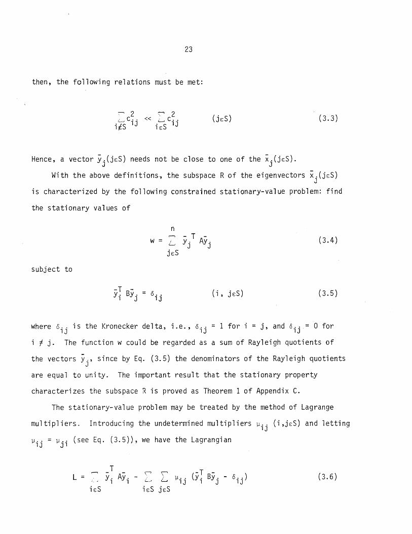
then, the following relations must be met:
\"' 2 L.. c ..
. S lJ ls
(jsS)
Hence, a vector Yj(jsS) needs not be close to one of the xj(jsS).
(3.3)
With the above definitions~ the subspace R of the eigenvectors x.(jsS) J
is characterized by the following constrained stationary-value problem: find
the stationary values of
subject to
n ~ - T -w = L_, y. Ay.
J J jsS
-T - = y. By. o .. 1 J lJ
(3.4)
(i, jsS) (3.5)
where Qij is the Kronecker delta, i.e., Qij = 1 for i = j, and Qij = 0 for
i f j. The function w could be regarded as a sum of Rayleigh quotients of
the vectors y., since by Eq. (3.5) the denominators of the Rayleigh quotients J
are equal to unity. The important result that the stationary property
characterizes the subspace R is proved as Theorem 1 of Appendix C.
The stationary-value problem may be treated by the method of Lagrange
multipliers. Introducing the undetermined multipliers ~ij (i ,jsS) and letting
11·· = 11·' (see Eq. (3.5)), we have the Lagrangian lJ Jl
T (- T -
AY· \' '\"' By. Q .. ) (3.6) L = y. - L 11· . y. -/ •. _r 1 1 L--- lJ 1 J lJ isS isS jsS

24
The problem of Eqs. (3.4) and (3.5) is equivalent to that of solying the
unconstrained stationary-value problem for the Lagrangian L. The problem
is solved setting the first partial derivatives of L with respect to the
unknowns y. and ~ .. equal to zero, i.e., J lJ
aL = 0 -'Oy.
J
~=O a~ ..
lJ
AY· = L ~ .. By. J 1 J 1
isS
-T -y. By. = o .. 1 J lJ
Introducing the following notation
o = (d ,d , ... ,d ) PI P2 Ps
we can write Eq. (3.7) in matrix form as
AY· = Bya. J J
or collectively
AY = BYD
(j sS) (3.7)
(i,jsS) (3.8)
(3.9)
(3.10)
(3.11)

25
In the same way, Eq. (3.8) can be written as
(3.12)
where Is is the unit matrix of order s. Hence, the subspace R of the
desired eigenvectors can be found by solving Eqs. (3.11) and (3.12). Note
that Eqs. (3.11) and (3.12) are nonlinear in 0 and Y and that there are
s (s + 1)/2 scalar unknown elements in 0, since 0 is symmetric, and
s (s + 1)/2 independent equations in Eq. (3.12). In the next section, the
solution of Eqs. (3.11) and (3.12) in the special case that (jsS) are all
multiple or close eigenvalues will be discussed.
3.3 The Iterative Scheme
In this section, the application of the Newton-Raphson technique to
the solution of Eqs. (3.11) and (3.12) for multiple or close eigenvalues
and their corresponding eigenvectors will be presented. To simplify the
notation in this discussion, we take the set S = [1,2, ... ,sJ, that is, the
s lowest eigenvalues are close together, or the multiplicity of the lowest
eigenvalue is s. It should be emphasized that this is not restrictive, and
the procedure is perfectly applicable to multiple or close eigenvalues in
any range.
Assume that the initial values for 0 and Y, 0(0) and y(O) are available
(the solution for the initial values will be discussed in Chapter 4).
Furthermore, we assume that the initial vectors in y(O) are in the neighbor
hood of the subspace of the eigenvectors X = [xl ,x2 , ... ,xs J and that they

26
T have been orthonormalized with respect to the matrix B, i.e., y(O)BY(O) = I .
s
With the above assumptions, we now apply the Newton-Raphson technique to the
solution of Eqs. (3.11) and (3.12). For the general kth iteration step, let
(3.13)
where ~a.(k) and ~y.(k) are unknown incremental values for d.(k) and y.(k). J J J J
Introducing Eq. (3.13) into Eqs. (3.10) and (3.12) and neglecting the
nonlinear terms, we obtain the linear simultaneous equations for ~a.(k) and J
(3.14)
(3.15)
By Theorem 3 of Appendix C, if the A. (j = 1,2, ... ,s) are multiple or J
close eigenvalues, the off-diagonal elements of 0 are zero or very small
compared with its diagonal ones, thus the last term of Eq. (3.14) may be
. t d b B - (k) . ld· approxlma e y ~jj ~Yj ,Yle lng
Let us take
(3.17)

,...,.., L/
Then, Eq. (3.15) becomes
(3.18)
which is the condition that the incremental vectors be orthogonal to the
current vectors with respect to B. If the computational scheme is slightly
altered so that the latest y. (k) is used at all times, the orthogonality 1
condition is satisfied automatically provided that the initial vectors y.(O) 1
are orthogonal. What this means is that we use y. (k) (i = 1,2, ... ,j - 1) 1
for the computation of y.(k+1). J
The final equations to solve for ~a.(k) and ~y.(k) are Eqs. (3.16) J J
and (3.18) along with the orthonormality condition, Eq. (3.17). These
equations can be written in matrix form as
A - 11 •• (k)B _ By(k) - (k) - (k) ~y. - rj
JJ J
-- --- .- - (3.19)
T ~a . (k) _ y(k) B 0 0
J
where
- (k) r. J
(3.20)
The coefficient matrix for the unknowns, dj(k) and Yj(k), is symmetric.
Furthermore, it is nonsingular, as is shown in Appendix A. Thus, Eq. (3.19)

28
can be solved for ~a.(k) and 6y.(k), yielding improved values, a.(k+1) and J J J
- (k+ 1) y j from Eq. (3. 13) .
The algorithm using Eq. (3.19) requires a new triangularization in
each iteration, since the coefficient matrix is changed in each iteration.
It therefore seems useful, as in Chapter 2, to substitute (A - ~ .. (0)8) for JJ
(A - ~jj(k)B) in Eq. (3.19) in order to save computational effort in the
solution. That is, the basic equations for the increments are taken as
= -.- - _ .. - (3.21)
o o
where the residual vector r.(k) is defined as in Eq. (3.20). The coefficient J .
matrix in Eq. (3.21) is also symmetric and nonsingular (Appendix A). The
equation (3.21) was obtained discarding a small linear term (~ .. (k) -JJ .
(0) ~ (k) ~.. )8 y. of Eq. (3.19). The procedure using Eq. (3.21) requires only
JJ J
partial triangularizations in each iteration, since only the vectors in
y(k) are changed, reducing the number of operations per iteration. The pro
cedure depends, for its convenience, on the decoupling of the ~Yj(k) for the
s vectors y.(k) (i=1,2, ... ,s). The decoupling was possible only because J
the small linear terms
i=l ifj

29
(see Eq. (3.14)) could be dropped for A. (j=l, 2, ... , s) all close J
together. Experience with Eq. (3.21) for A. (j=l, 2, ., s) vihich are not J
close together indicates that satisfactory results cannot be obtained.
Note that if s = 1, Eqs. (3.19) and (3.21) are equivalent to the
equations used for distinct eigenvalues and corresponding eigenvectors:
Eq. (3.19) becomes Eq. (2.6), the equations used in the Robinson-Harris
method, and Eq. (3.21) becomes Eq. (2.7), used in the proposed method.
With sufficient large k, the incremental values ~a.(k) and ~y. (k) J J
will vanish. Then, from Eq. (3.21)
Letting
1 i m r. ( k) = 1 i m (AY. ( k ) k-)-OO J k~ J
lim d.(k) dj = k-tco J
- _limy.(k) Yj - k-tco J
we write Eqs. (3.22) and (3.17) as
AY = BYD
(3.22)
(3.23)
(3.24)
where Y = (Y1'Y2'··· 'Ys), and 0 = (d 1,d2,···,ds )· By Theorem 3 of Appendix C,
if the eigenvalues A. (j=1,2, ... ,s) are multiple, the values of the off-J
diagonal elements of 0 are all zero, and its diagonal elements have an equal

30
value which is the desired multiple eigenvalue. Moreover, the vectors in
Yare the corresponding eigenvectors. However, if the eigenvalues are
close but not equal, additional operations are required to find the desired
eigenvalues and eigenvectors. These additional operations are the subject
of the next section.
3.4 Treatment of Close Roots
Once the converged solution 0 and Y has been found by the algorithm
described in the previous section, but the values of the off-diagonal
elements of 0 are not zero, the vectors in Yare rotated in the subspace
of Y to find the true eigenvectors. A rotation matrix is found by solving
a small eigenvalue problem. Furthermore, the eigenvalues of the small
eigenvalue problem are the desired eigenvalues. The derivation of the
small eigenvalue problem is as follows. The system with the s eigenvectors
in X = [x l ,x2,··.,xs J and corresponding eigenvalues in A = diag (A 1,A2,··· ,AS)
may be written as
AX = BXA (3.26)
where A and B are symmetric matrices of order n. Now, let
x = YZ (3.27)
where Z is the unknown rotation matrix of order s. Introducing Eq. (3.27)
into Eq. (3.26), we get
AYZ = BYZA (3.28)

31
Postmultiplying Eq. (3.24) by the matrix Z yields
AYZ = BYDZ (3.29)
Premultiplying Eqs. (3.28) and (3.29) and using yTBY = Is of Eq. (3.25), we
obtain the special eigenvalue problem of order s
DZ = ZA (3.30)
where D is the converged solution found by the algorithm of the previous
section. The matrix D is symmetric (see Eq. (3.24)) and of order s, the
number of close eigenvalues, which is usually small. The absolute values
of the off-diagonal elements of D are small compared with those of its
diagonal elements (see Appendix C). The eigenvalue problem, Eq. (3.30) can
be easily solved by any suitable technique such as Jacobi's method [31,51J,
yielding the desired eigenvalues in A (AI' A2' . , As) and the matrix Z,
which in turn gives the eigenvectors X by Eq. (3.27). The number of oper
ations required for the solution of Eq. (3.30) is very small compared with
that of Eq. (3.21), since s is small.
3.5 Convergence Rate and Operation Count
In this section, the convergence rates of a multiple eigenvalue and
the corresponding eigenvectors found in Appendix B will be summarized. For
convenience, we assume that the lowest eigenvalues are multiple, i.e.,
* L t th . t· t - ( k) (. - 1 2 ) A = Al = A2 = ... = As' e e approxlma e elgenvec ors Yj J - , , ... ,s
be expanded in terms of the ei genvectors xi (i = 1, 2, . . . , n), i. e. ,

32
n
Y-.(k) = \"'
J i .. J
c .. (k) X. lJ 1
j = 1, 2, ... , s (3.31) ;=1
where cij(k) is a scalar representing the components of the eigenvector xi
on y- .(k). If y.(k) denotes the error in (k) and e.(k) the error in y- .(k), J J lljj J J
then they may be defi ned by
( k) y. =
J * A
r n 17[ s -I t \"' ( k lJ 1 /2 \" ( k 1 2
Jl1 /2
, L (c.. ') (c.. ') ! ' 1 J 1 J Li=s+l i=l
(3.32)
(3.33)
As shown in Appendix B, the error in ~jj(k+l) and ;j(k+l) m~ be written as
where
h = m~x i
(k+1 ) y. =
J
e.(k+1) = he.(k) J J
A*- ll"(O) I JJ 1 I ()) «
A. - u.!.!\V I 1 . JJ I
i=s+1,s+2, ... , n;
j=l, 2, ... , S
(3.34)
(3.35)
(3.36)

33
t can be seen from Eqs. (3.34) and (3.35) that the eigenvalues and the
corresponding eigenvectors converge linearly. However, the eigenvalues
converge much more rapidly than the eigenvectors.
The number of operations Np required for finding multiple or close
eigenvalues and the corresponding eigenvectors is calculated in Table 1.
Th is number is
N = 1 pn (m2 + 3m + 2mb + 2) + T n [( s + 4) rna + 2mb + 12 (s 2 + 7s + 4) ] (3.37) p 2 a a p
where s is the multiplicity of an eigenvalue or the number of close eigen
values, and Tp is the total number of iterations required for a solution.
It can be seen that if s = 1, the number of operations is equal to the number
of operations required for finding a simple eigenvalue and the corresponding
eigenvector (see Eq. (2.14)).

34
4. APPROXIMATE STARTING EIGENSOLUTION
4.1 General
The iterative methods described in the previous chapters begin with an
approximate starting eigensolution. In this chapter, a procedure to find
the starting solution is presented. The approximate starting solution of
an eigenvalue problem is often available either as the final answer in some
approximate methods or as an intermediate result in other iterative methods.
Numerous methods for approximate solutions have been developed. These
include static or dynamic condensation [2,3,25,28,34,42J, Rayleigh-Ritz
analysis [48,51J, component mode analysis [9,51J, and related methods sum
marized by Uhrig [50J. In all these methods, the approximate solution is
found in a single step, and not in an iterative process. Hence, automatic
improvement of the solution is not built into the procedure. Moreover, the
success of the methods depends, to a great extent, on the engineer's judg
ment, which is difficult to incorporate into an automatic computer program.
Another possible way for finding the approximate solution is to take
the intermediate results from other iterative methods such as a method
combining the Gran-Schmidt orthogonalization process [51J with simultaneous
iteration method or combining Rayleigh-Ritz analysis [6,9,11,29,32,49J with
simultaneous iteration method. The latter combined method is sometimes
called the "subspace iteration rrethod" [6,9J. The subspace iteration method
is used here to find approximate starting solutions because it has a better
convergence rate than most others. The method itself turns out to require
selecting starting vectors. However, a scheme to find starting vectors for

35
the subspace iteration method has been well established and is fairly routine
(see Section 4.2.2). In the next section, the subspace iteration method will
be di scussed.
4.2 Subspace Iteration Method
4.2.1 The Iterative Scheme
The subspace iteration method is a repeated application of the
classical vector iteration method (power method) and Rayleigh-Ritz analysis.
Suppose that the p smallest eigenvalues A. (i = 1,2, ... ,p) and corresponding 1
eigenvectors x. are required and that we have p initial independent vectors 1
- (0) (. - 1 2 ) . d . . 1 b . th . h b h d xi 1 - " ..• ,p spannlng a p- lmenSlona su space ln e nelg or 00
of the subspace of the desired eigenvectors.
If the approximate eigenvectors and corresponding eigenvalues after k
iterations are denoted by x.(k) and Ao (k), X(k) = [x1(k), x2
(k) , ... ,x (k)J, 1 1 p
(k) . (k) (k) (k) and 0 = dlag (AI ' A2 , ... ,Ap ), the subspace iteration method for
the kth iteration may be described as follows:
(i) Find the improved eigenvectors y(k) = [Y1 (k), Y2(k) , ... ,Yp (k)]
by the simultaneous inverse iteration method;
(4.1)
(ii) Compute the projections of the operators A and B onto the
subspace spanned by the p vectors in y(k);
A(k) = y(k)T Ay(k)
g(k) = y(k)T By(k) (4.2)

Then,
36
where A(k) and S(k) are pxp symmetric matrices.
(iii) Solve the eigenvalue problem of reduced order p for the
eigenvalues in D(k) = diag (A1(k), A2(k) , ... ,Ap(k) and the
eigenvectors in Z(k) = [Zl(k), Z2(k) , ... ,Zp(k)];
(iv) Find an improved approximation to the eigenvectors;
lim O(k) = k~
lim X(k) = k~
(4.3)
(4.4)
(4.5)
Note that Eqs. (4.2) through (4.4) represent a Rayleigh-Ritz analysis with
the vectors in y(k) as the Ritz basis vectors, which results in x(k), the
best approximation to the true eigenvectors in the subspace of y(k).
More rapid convergence can be obtained by taking more iteration vectors
than the number of eigensolutions sought. However, the more starting
vectors are taken, the more computational effort is required per iteration.
As an optimal number of iteration vectors, q, q = min (2p, p + 8) has been
suggested [6,9J.

37
Metz Referenoe Room Civil Engineering Departman~
BI06 C.E. Building T~4~a~~4+~ n~ Tl14"~~_ UU~YV.U.VJ v. ~~~_~w~~
Urbana,,111ino1a 6180ll
To find eigenvalues within a given range a < ~ < b and the correspond
ing eigenvectors, we may use, instead of Eq. (4.1), the inverse iteration
with a shift [32J:
(A - ~B) y(k) = BX(k-1) (4.6)
where ~ is a shift and can be taken as (a + b)/2. It is clear from Eq. (4.6)
that the eigenvectors corresponding to the eigenvalues in the vicinity of a
shift ~ will converge rapidly. However, the convergence of other eigen
vectors may be slower than when the shift is not applied, since as a result
of the application of the shift, the absolute values of some shifted eigen-
values may become closer.
4.2.2 Starting Vectors
The number of iterations required for convergence depends on how
close the subspace spanned by the starting vectors is to the exact subspace.
If approximations to the required eigenvectors are already available, e.g.,
from a previous solution to a similar problem, these may be used as a set
of starting vectors. If not, we may use one of the schemes for generating
starting vectors which have been proposed as effective [6,11,32,47J.
The scheme for establishing the starting vectors proposed by Bathe and
Wilson [6,9J is used here because of its simplicity and effectiveness. The
scheme may be described as follows. The first column of BX(O) in Eq. (4.1)
is formed simply from the diagonal elements of Bo That is, if BX(O) is
denoted by C,
= b .. 11
(i = 1,2, ... ,n) (4.7)

38
This assures that all mass degrees-of-freedom are excited in or~er not to
miss a mode [6,9J. The next (q-1) columns in C may each have all zeros
except for a certain coordinate where a one is placed. These coordinates
are found in the following way. First, compute the ratios a.·/b .. 11 1 1
(i = 1,2, ... ,n) and take the (q-1) s"s (j = 1,2, ... ,q-1) such that the J
absolute values of the ratios aiilb ii for i (i = sl' s2,···,Sq_1) are
smallest over all i. Then,
c· = 1 for = s . ( i = 1,2, ... ,n) 1 , j-1 J
= 0 for i ~ s. (j = 1,2, ... ,q-1) (4.8) J
If the absolute values of the ra ti os are close or equal, then it was recom-
mended [6,9J that the s .IS (j = 1,2, ... ,q-l) be chosen so that they are well J
spaced.
4.2.3 Convergence Rate, Operation Count, and Estimation of Errors
With an adequate choice of the starting vectors, the subspace
iteration method gives good approximations to the exact eigenvalues and
eigenvectors even after only a few iterations. However, the subsequent
convergence is only linear with the rates of convergence equal to
Ai/Aq+1 (i = 1,2, ... ,p) for the ith eigenvector and (Ai /Aq+1)2 for the
corresponding eigenvalue. These ratios indicate that for the higher eigen-
value convergence is slower. Hence, the convergence of the pth mode controls
the termination of the iteration process.
39
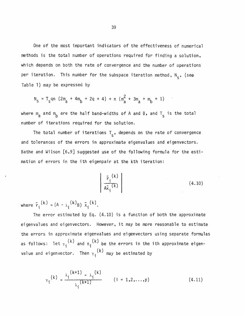
One of the most important indicators of the effectiveness of numerical
methods is the total number of operations required for finding a solution,
which depends on both the rate of convergence and the number of operations
per i terati on. This number for the subspace iteration method,N , (see s
Table 1) may be expressed by
where rna and mb are the half band-widths of A and B, and Ts is the total
number of iterations required for the solution.
The total number of iterations T , depends on the rate of convergence s and tolerances of the errors in approximate eigenvalues and eigenvectors.
Bathe and Wilson [6,9J suggested use of the following formula for the esti-
mation of errors in the ith eigenpair at the kth iteration:
where r. (k) = (A - A. (k)B) x. (k). 1 , 1
- (k) r. 1
- ( k) Ax. 1
(4.10)
The error estimated by Eq. (4.10) is a function of both the approximate
eigenvalues and eigenvectors. However, it may be more reasonable to estimate
the errors in approximate eigenvalues and eigenvectors using separate formulas
as follows: let Yi (k) and 8i (k) be the errors in the ith approximate eigen
value and eigenvector. Then y. (k) may be estimated by 1
A. (k+ 1) _ A. (k) y. ( k ) ~ _, __ .,....---=---, __
1 A.(k+1) 1
(i = 1,2, ... ,p) (4.11)

40
For the estimate of 8,. (k) , we find the incremental vectors ~x. (k) from the , ,
re 1 a ti ons
X. (k+l) = a .. (k)x. (k) + ~x. (k) , ", ,
T X. (k) B ~x. (k) = 0 , , ( 4. 12)
Then,
(4.13)
If some of the approximate eigenvalues Ai (i = PI' P2'··· ,ps) are equal or
very close, we may then compute ~Xi (k) from the relations
T Xj (k) Bt;x; (k) = 0 ; (j = Pl'P2'··· ,ps)
(k) (- (k)T - (k))1/2 (Ps 2 (k)- (k)T _ (k))1/2 8 . ::: X • B X· La. . X • B X
J'
, " lJ J j=p
1
(4.14)
For the purpose of comparison of the proposed methods of Chapters 2 and 3
with the subspace iteration method, the errors were computed using Eqs.
( 4. 11) to (4. 14 ) .

41
4.3 Starting Solution for the Proposed Method
The intermediate results from the subspace iteration are used as the
starting solutions for the proposed method. During the subspace iterations,
the errors in approximate eigenvalues and corresponding eigenvectors can be
estimated by the scheme described in Section 4.2.3. Furthermore, these
errors can be used for estimating the number of iterations or the number of
operations required for the solution by both the subspace iteration method
and the proposed method. Hence, it is possible to estimate the optimal
number of iterations to be carried out by the subspace iteration method.
This optimal number of iterations is usually one or two.
Let A~ and x~ (i = 1,2, ... ,p) be the intermediate solutions from the
subspace iteration method after the optimal number of iterations. Then, if
* * -* the A. are well separated, A. and x. can be taken as the starting solutions 1 1 1
for the method of Chapter 2, A'(O) and i.(O). However, if some of them, 1 1
* (. ) 1 close, "\ *. and x-*. t k e.g., Ai 1 = PI ,P2'··· 'Ps are equa or very 1\1 1 are a en as
the starting solution for the method of Chapter 3 as
y. (O) = x-* 1 i
(0) = A~ ~ii 1
(0) ~. . = 0 for i f j 1J
42
It should be noted that from Eqs. (4.3) and (4.4), the ite~ation
vectors in the subspace iteration method are always orthogonalized with
respect to B. Therefore, orthogonal;zation is not required for the first
iteration of the proposed method.

43
5. NUMERICAL RESULTS AND COMPARISONS
5.1 General
The relative efficiency of the methods developed in this study is
illustrated in this chapter by the numerical results of the free vibration
analyses of the following example problems:
(a) Ten-Story, Ten-Bay Plane Frame
(b) Two-Hinged Circular Arch
(c) Simply Supported Plate.
The problems were formulated using a stiffness method for the plane frame
problem, a finite difference method for the arch problem, and a finite element
method for the plate problem. No attempt has been made to present the
solutions of eigenvalue problems of very large order, although the proposed
method is developed for them. However, some trends can be inferred from the
example problems presented here.
The first two problems, with distinct eigneva1ues, were solved by the
method discussed in Chapter 2 and the third one, with multiple or close
eigenvalues, by the method of Chapter 3. The above problems were also solved
using the Robinson-Harris method [44J and the subspace iteration method
discussed in Chapter 4. The results are summarized in Tables 2 through 5. The
numerical results given here are shown to be consistent with the convergence
estimates of Appendix B.
For each method, the total number of operations required for finding the
desired eigenvalues and eigenvectors to the same accuracy was found. These -4 are presented and compared in Table 6. Although a tolerance of]O on the
eigenvalues and eigenvectors should be sufficient for normal requirements, it

44
was taken as 10-6 for the purpose of comparisons of the convergence character-
istics of the methods.
The numerical computations of the above problems were performed on the
CDC CYBER 175 system of the Digital Computer Laboratory of' the University of
Illinois, Urbana, Illinois.
5.2 Plane Frame
The ten-story, ten-bay plane shown in Fig. 2 was taken as an example
problem in order to test the method of Chapter 2 for problems with distinct
eigenvalues. The problem was formulated by a stiffness method in which the
axial deformations of the members are considered, but the shear deformations
neglected [40J. The frame with three displacements per joint has a total of
330 degrees of freedom. The mass matrix is the consjstent mass matrix [4,5J
with a maximum half-bandwidth of 35, equal to that of the stiffness matrix.
The four smallest eigenvalues and their corresponding eigenvectors
were computed by the proposed method, by the Robinson-Harris method, and by
the subspace iteration method. The results are given in Table 2. For the
subspace iteration method, ten starting vectors were formed by the technique
suggested by Bathe and Wilson (see Section 4.2.2). The starting approximate
eigenvalues and eigenvectors for the proposed method and for the Robinson-
Harris method were established by performing two cycles of subspace iteration.
Table 2 shows that even the eigenvalues calculated by two subspace iterations
are already However, the eigenvectors are accurate
to only one or two figures. In addition, the convergence of eigenvectors by
the subspace iteration method is so slow, as discussed in Section 4.2.3, that
12 iterations were required for the convergence of both eigenvalues arid eigen-

45
vectors to the indicated tolerance. The proposed method and the Robinson~
Harris method required only two iterations for the convergence of eigenpairs
except for that of the fourth mode, which required four iterations by the
proposed method and three iterations by the Robinson-Harris method.
The total number of operations to solve for all the desired eigenpairs by
the proposed method is 3.50xl06; by the Robinson-Harris method, 4.57xl06 , and
by the subspace iteration method, 9.27xl06. Therefore, the Robinson-Harris
method required 1.31 times as many operations as the proposed method did, and
the subspace iteration method required 2.78 times as many operations, as shown
in Table 6.
5.3 Arch
A uniform 90 degree circular arch simply supported at both ends was
analyzed for in-plane vibration behavior. The arch has the radius a and the
thickness h, and the ratio a/h = 20. Melin and Robinson [36J investigated the
free vibration behavior of such an arch as a part of a study of vibrations of
a simply supported cylindrical shell using a finite difference method. The
arch was divided into 12 uniform segments giving 22 degrees of freedom. The
maximum half-bandwidth of the stiffness matrix is four and the mass matrix is
a unit diagonal matrix.
The problem was analyzed for the three smallest eigenvalues and their
eigenvectors by the proposed method, by the Robinson-Harris method, and by the
subspace iteration method. The results are summarized in Table 3. Five radial
displacements were taken as master displacements for the iteration vectors of
the subspace iteration method. Starting approximate eigenpairs for the proposed
method and the Robinson-Harris method were established by carrying out just
one cycle of the subspace iteration.

46
The comparison of the total number of operations for each method is
given in Table 6. The proposed method needed 8.87xl03 operations, the
Robinson-Harris method 9.77x.03 operations, and the subspace iteration method
1.76xl04 operations. Hence, the ratio of the total number .of operations by
the Robinson-Harris method to that by the proposed method is 1.10, and this
ratio for the subspace iteration method is 1.98.
5.4 Plate Bending
A plate simply supported on all edges was analyzed in order to test the
method presented in Chapter 3, for the solution of eigenvalue problems with
multiple or close eigenvalues. The plate has the lengths a and b, and the
theckness h. Two special cases were considered; an aspect ratio bla of 1.00
and bla equal to 1.01. The first case gives multiple roots, while the second
one gives close roots. The problem was formulated by a finite element method,
in which the plate was divided into 16 elements. Each unrestarined node has
a deflection and two rotational displacements, giving a total of 39 degrees of
freedom. The mass matrix is the consistent mass matrix [4,5J with a maximum
half-bandwidth of 16, equal to that of the stiffness matrix.
The four smallest eigenvalues and corresponding eigenvectors were computed
for both cases by the proposed method and by the subspace iteration method.
The results are summarized in Tables 4 and 5. the deflection at each node was
taken as the master degrees of freedom, giving nine iteration vectors for the
subspace iteration method. Only one cycle of subspace iteration was performed
for the proposed method. The multiple eigenvalues of the square plate
close eigenvalues of the rectangular plate were isolated by the method
discussed in Chapter 3.

47
The total number of operations by the proposed method for both cases is
1 .27xl05 and by the subspace iteration method, 2.20xl05, as shown in Table 6.
Hence, the subspace iteration method needed 1.73 times as many operations as
the proposed method did.
5.5 Comparison between the Theoretical Convergence Rates and Numerical
Results
It was shown in the previous chapters that in the proposed method, the
convergence of eigenvalues is much faster than that of eigenvectors. Hence,
the convergence of the eigenvectors governs the termination of process, when
the tolerances on the eigenvalues and eigenvectors are same. Comparison
between the theoretical convergence rates and numerical results was, therefore,
carried out only for the eigenvectors. Comparisons between the proposed
method and subspace iteration method are given in Tables 7, 8, and 9.
The numerical convergence rates were computed by e~k+l)/e~k), where
e~k) is the error on the ith approximate eigenvector at the kth iteration.
These errors are given in Tables 2 through 5, showing that the numerical
convergence rates for the proposed method and the subspace iteration method
increase monotonically to approach the theoretical convergence rates as the
number of iterations increases. A typical example for this is the convergence
rates of the fourth eigenvector of the frame problem, as shown in Table 7.
The number of iterations for this mode is large enough to provide a good
comparison between the theoretical and numerical convergence rates.
Tables 7, 8, and 9 show that in the proposed method, eigenpairs
much faster than in the subspace iteration method. Note also that in Table 9,
the numerical convergence rates for the proposed method are almost same as

48
those rates for the problem with double roots. Hence~ the expressions for the
theoretical convergence rates for multiple eigenvalues also seem applicable to
the case of close eigenvalues.

49
6. SUMMARY AND CONCLUSIONS
6.1 Summary of the Proposed Method
Two iterative procedures for the solution of linear eigenvalue problems
for systems with a finite number of degrees of freedom were discussed in
Chapters 2 and 3. Chapter 2 developed a procedure for finding distinct
eigenvalues and the corresponding eigenvectors, and Chapter 3 dealt with
multiple or close eigenvalues and the corresponding eigenvectors.
For distinct eigenvalues and the corresponding eigenvectors, the Robinson
Harris method [44J was modified to save overall computational effort by the
use of a II modified" form of the Newton-Raphson technique. The modified method
reduces both the number of operations per iteration and the convergence rates.
However, the reduction of the number of operations generally compensates for
the disadvantage of the decrease of the convergence rate, reducing the total
number of operations.
The procedure in Chapter 2 for finding a distinct eigenvalue and the
corresponding eigenvector fails if the eigenvalue is one of multiple or close
eigenvalues, because the matrix involved in the computation become ill-condi
tioned. This difficulty has been overcome by the new method of Chapter 3. In
this mehtod, all eigenvalues close to an eigenvalue or a multiple eigenvalue
and the corresponding eigenvectors are found in a group. In other words, a
subspace spanned by the approximate eigenvectors is projected by iterations
onto the subspace of the exact eigenvectors. If the eigenvalues are multiple,
the vec~ors spanning the subspace are exact eigenvectors. However, if the
eigenvalues are close, the exact eigenvectors are found by a simple rotation
of the vectors in the subspace. The rotation matrix is found from a special

50
eigenvalue problem of small order s, the number of the close eigenvalues.
The eigenvalues of the small eigenvalue problem are exact eigenvalues of the
original system.
The above procedures of the successive approximations require initial
approximations to the eigenvalues and eigenvectors. These are available
either as the final solution in some approximate methods such as static or
dynamic condensation or as an intermediate result in an iterative method as
the subspace iteration method described in Chapter 4.
6.2 Conclusions
The method presented in this study is very efficient for finding a limited
number of soltutions of eigenvalue problems of large order arising from the
linear dynamic analysis of structures. The features of the method are summarized
as follows.
(a) The method has very high convergence rates for eigenvalues
and eigenvectors. The method is more economical than the
subspace iteration method, the advantage being greater
in larger problems. For comparable accuracy, a ten-story
ten-bay frame required only 36% of the number of operations
need in applying subspace iterations.
(b) A transformation to the special eigenvalue problem is not
required. Thus, the characteristics of the given matrices
such as the sparseness, bandness, and symmetry are preserved,
mi~imizing the storage requirements and the number of
operations.

51
(c) Any number of multiple or close eigenvalues and their
eigenvectors can be found. The existence of the multiple
or close eigenvalues can be detected during the iterations
by the method of Chapter 2.
(d) The eigenvalues in any range of interest and their
eigenvectors can be found, if approximations to the
solution are known.
(e) The solution can be checked to determine if some eigenvalues
and corresponding eigenvectors of interest have been
missed, without extra operations.
6.3 Recommendations for Further Study
Several possible areas of further study to improve the proposed method
may be suggested.
(a) The convergence rate may be improved by other modifica
tions of the successive approximation method used for
the proposed method.
(b) Further improvements may be possible for the method of
finding an initial approximation to the eigensolution,
and for isolating the eigenvalues and their eigenvectors
which may be missed by the proposed method.
(c) The proposed method may be applied to other practical
problems of our interest such as a stability analysis of
structures.
(d) The proposed method could be easily extended to the contin-
uous eigenvalue problems if there were better ways of
direct estimation of their eigensolutions.
52
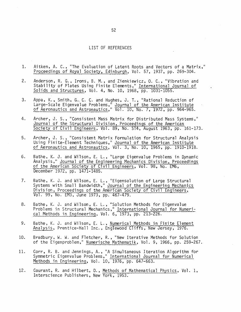
LIST OF REFERENCES
1. Aitken, A. C., liThe Evaluation of Latent Roots and Vectors of a Matrix," Proceedings of Royal Society, Edinburgh, Vol. 57, 1937, pp. 269-304.
2. Anderson, R. G., Irons, B. M., and Zienkiewicz, O. C., "Vibration and Stabi 1 i ty of Pl ates Us i ng Fi ni te El errents, II Interna ti ona 1 Journal of Solids and Structures, Vol. 4, No. 10, 1968, pp. 1031-1055.
3. Appa, K." Smith, G.o C. C. and Hughes, J. T., "Rational Reduction of Large-Scale Eigenvalue Problems," Journal of the American Institute of Aeronautics and Astronautics," Vol. 10, No.7, 1972, pp. 964-965.
4. Archer, J. S., "Consistent Mass Matrix for Distributed Mass Systems," Journal of the Structural Division, Proceedings of the American Society of Civil Engineers, ~ol. 89, No. ST4, August 1963, pp. 161-173.
5. Archer, J. S., "Consistent Matrix Formulation for Structural Analysis Using Finite-Element Techniques," Journal of the American Institute of Aeronautics and Astronautics, Vol. 3, No. 10, 1965, pp. 1910-1918.
6. Bathe, K. J. and Wilson, E. L., "Large Eigenvalue Problems in Dynamic Analysis," Journal of the Engineering Mechanics Division, Proceedings of the American Society of Civil Engineers, Vol. 98, No. EM6, December 1972, pp. 1471-1485.
7 . Bat he, K . J. and Wi 1 son, E . L., II E i g ens 0 1 uti 0 n 0 f La rg e S tr u c t u ra 1 Systems with Small Bandwidth," Journal of the Engineering Mechanics Division, Proceedings of the American Society of Civil Engineers, Vol. 99, No. EM3, June 1973, pp. 467-479.
8. Bathe, K. J. and Wilson, E. L., IISol ution Methods for Eigenvalue Problems in Structural Mechanics,1I International Journal for Numerical Methods in Engineering, Vol. 6, 1973, pp. 213-226.
9. Bathe, K. J. and Wilson, E. L., Numerical Methods in Finite Element Analysis, Prentice-Hall Inc., Englewood Cliffs, New Jersey, 1976.
10. Bradbury, w. w. and Fletcher, R., "New Iterative Methods for Solution of the Eigenproblem," Numerische Mathematik, Vol. 9, 1966, pp. 259-267.
11. Corr, R. B. and Jennings, A., "A Simultaneous Iteration Algorithm for Symmetric Eigenvalue Problems," International Journal for Numerical Methods in Engineering, Vol. 10, 1976, pp. 647-663.
12. Courant, R. and Hilbert, D., Methods of Mathematical Physics, Vol. 1, Interscience Publishers, New York, 1953;

53
13. Crandall, S. H., IIIterative Procedures Related to Relaxation Methods for Eigenvalue Problems," Proceedings of Royal Society, London, A207, 1951~ pp. 416-423.
14. Crandall, S. H., Engineering Analysis, McGraw-Hill Book Co., Inc., New York, 1956.
15. Dong~ S. B. and Wolf, J. A., Jr., "On a Direct-Iterative Eigensolution Technique," International Journal for Numerical Methods in Engineering, Vol. 4, 1972, pp. 155-161.
16. Faddeev, D. K. and Faddeeva, V. N., Computational Methods of Linear Algebra, W. H. Freeman and Co., San Francisco and London, 1963.
17. Felippa, C. A., ilRefined Finite Element Analysis of Linear and Nonlinear Two-Dimensional Structures," Ph.D. thesis, University of California, Berkeley, Department of Civil Engineering, 1966.
18. Fox, R. L. and Kapoor, M. P., IIA Minimization Method for the Solution of the Eigenproblem Arising in Structural Dynamics,1I Proceedings of the Second Conference on Matrix Methods in Structural Mechanics, Wright-Patterson Air Force Base, Ohio, AFFDL-TR-68-150, 1968, pp. 332- 345.
19. Francis, J. G. F., "The OR Transformation, Parts I and 11,11 Computer Journal, VoiD 4, 1961, pp. 265-271, Vol. 4, 1962, pp. 332-345.
20 . F r i ed, I., II 0 P t i rna 1 G r ad i en t Min i m i z a t ion Sc heme for Fin i teE 1 erne n t Eigenproblems,I' Journal of Sound and Vibration, Vol. 20, 1972, pp. 333- 342.
21. Givens, J. W., "Numerical Computation of the Characteristic Value of a Real Symmetric Matrix,1I Oak Ridge National Laboratory Report No. 1574, distributed by Office of Technical Services, Washington, D. C., 1954.
22. Gupta, K. K., "Vibration of Frames and Other Structures with Banded Stiffness Matrix," International Journal for Numerical Methods in Engineering, Vol. 2, 1970, pp. 221-228.
23. Gupta, K. K., "Eigenproblem Solution by a Combined Sturm Sequence and Inverse Iteration Technique," International Journal for Numerical Methods in Engineering, Vol. 7, 1973, pp. 17-42.
24. Guyan, R. J., IIReduction of Stiffness and Mass Matrices,1I Journal of the Arrerican Institute of Aeronautics and Astronautics,n Vol. 3, No.2, 19"65, pp. 380.

54
25. Henshell, R. D. and Ong, J. H., "Automatic Masters for Eigenvalue Economisation," Journal of Earthquake Engineering and Structural Dynamics, Vol. 3, 1975, pp. 375-383.
26. Householder, A. S., The Principles of Numerical Analysis, McGraw-Hill Book Co., Inc., New York, 1953. Republished by Dover Publications, Inc., 1974.
27. Irons, B. M., "Eigenvalue Economisers in Vibration Problems," Journal of the Royal Aeronautical Society, Vol. 67, August 1963, pp. 526-528.
28. Irons, B. M., "Structural Eigenvalue Problems: Elimination of Unwanted Variables," Journal of the American Institute of Aeronautics and Astronautics, Vol. 3, No.5, 1965, pp. 961-962.
29. Jennings, A., "A Di rect Iteration Method of Obtaining the Latent Roots and Vectors of a Symmetric Matrix," Proceedings of Cambridge Philosophical Society, Vol. 63, 1967, pp. 755-765.
30. Jennings, A., "~~ass Condensation and Simultaneous Iteration for Vibration Problems," International Journal for Numerical Methods in Engineering, V~l. 6, 1973, pp. 543-552.
31. Jennings, A., Matrix Computation for Engineers and Scientists, John Wiley & Sons, 1977.
32. Jensen, P. S., liThe Solution of Large Symmetric Eigenproblems by Sectioning," Journal of the Society for Industrial and Applied Mathematics, Numerical Analysis, Vol. 9, No.4, December 1972, pp. 534-545.
33. Lanczos, C., "An Iteration Method for the Solution of the Eigenvalue Problem of Linear Differential and Integral Operators," Journal of Research of the National Bureau of Standards, Vol. 45, 1950, pp. 255-282.
34. Leung, A. Y., \IAn Accurate Method of Dynamic Condensation in Structural Analysis," International Journal for Numerical Methods in Engineering, Vol. 12, 1978, pp. 1705-1715.
35. Meirovitch, L., Analytical Method in Vibration, The Macmillan Co., London, 1967.
36. Melin, J. W. and Robinson, A. R., liThe Analysis of the Dynamic Response to an Aboveground Simply Supported Cylindrical Shell Subjected to Blast Loading,1I Air Force System Command, Kirtland, Air Force Base, New Mexico, AFSWC-TR-61-55, August 1961.
37. Myskis, A. D., Advanced Mathematics for Engineers, MIR Publishers, Moscow, 1975.

55
38. Peters, G. and Wilkinson, J. H., IIEigenvalues ofAx=ABx with Band Symmetric A and B,II Computer Journal, Vol. 12, 1969, pp. 398-404.
39. Peters, G. and Wilkinson, J. H., IIAx=ABx and the Generalized Eigenproblem,1I Journal of the Society for Industrial and Applied Mathematics, Numerical Analysis, Vol. 7, No.4, December 1970, pp. 479-492.
40. Przemieniecki, J. S., IIMatrix Structural Analysis of Substructures," Journal of the American Institute of Aeronautics and Astronautics, Vol. 1, No.1, 1963, pp. 138-147.
41. Rall, L. B., II Newtons , Method for the Characteristic Value Problem AX=ABx," Journal of the Society for Industrial and Applied Mathematics, Vol. 9, No.2, June 1961.
42. Ramsden, J. N. and Stoker, J. R., "Mass Condensation: a Semi-Automatic Method for Reducing the Size of Vibration Problems," International Journal for Numerical Methods in Engineering, Vol. 1, 1969, pp. 333-349.
43. Rayleigh, Lord, The Theory of Sound, Second edition, Vol. 1, Macmillan Co., London, 1894. Republished by Dover Publications, Inc., 1945.
44. Robinson, A. R. and Harris, J. F., "Improving Approximate Eigenvalues and Eigenvectors," Journal of the Engineering Mechanics Division, Proceedings of the American Society of Civil Engineers, Vol. 97, No. EM2, April 1971, pp. 457-475.
45. Rosen, R. and Rubinstein, M. F., "Dynamic Analysis by Matrix Decomposition," Journal of the Engineering Mechanics Division, Proceedings of the American Society of Civil Engineers, No. EM2, April 1968, pp. 385-395.
46. Rutihauser, H. and Schwarz, H. R., "The LR Transformation Method for Symmetric Matrices," Numerische Mathematik, Vol. 5,1963, pp. 273-289.
47. Rutihauser, H., "Computational Aspects of F. L. Bauer's Simultaneous Iteration Method," Numerische Mathematik, Vol. 13, 1969, pp. 4-13.
48. Schwarz, H. R., Rutihauser, H. and Stiefel, E., Numerical Analysis of Symmetric Matrices, Prentice-Hall, Englewood Cliffs, New Jersey, 1973.
49. Schwarz, H. R., "The Eigenvalue Problem (A-AB)x=O for Symmetric Matrices of High Order," Computer Methods in Applied Mechanics and Engineering, Vol. 3, 1974, pp. 11-28.
50. Uhrig, R., "Reduction of the Number of Unknowns in the Displacement Method Applied to Kinetic Problems," Journal of Sound and Vibration, Vol. 4,1966, pp. 149-155.

56
51. Wilkinson, J. H., The Algebraic Eigenvalue Problem, Oxford ,University Press, London, 1965.
52. Zienkiewicz, O. C., The Finite Element Method in Engineering Science, Third edition, McGraw-Hill Book Co., Ltd., London, 1977.'
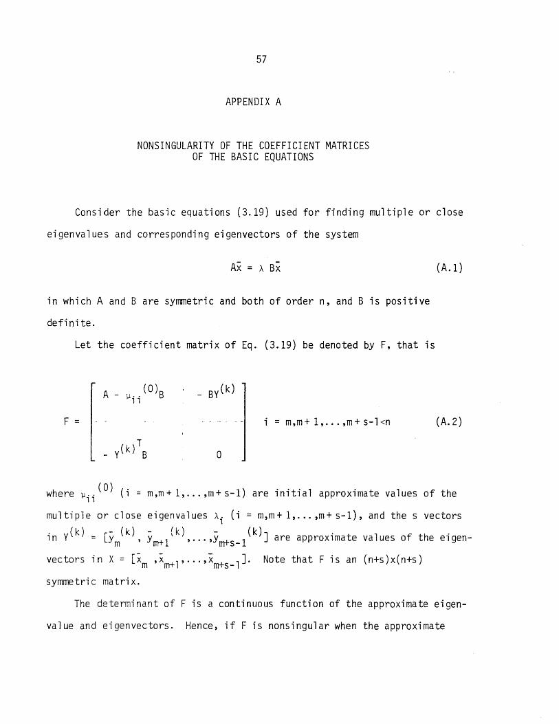
57
APPENDIX A
NONSINGULARITY OF THE COEFFICIENT MATRICES OF THE BASIC EQUATIONS
Consider the basic equations (3.19) used for finding multiple or close
eigenvalues and corresponding eigenvectors of the system
Ax = A Bx (A.1 )
in which A and B are symmetric and both of order n, and B is positive
defi ni te.
Let the coefficient matrix of Eq. (3.19) be denoted by F, that is
A - ~ .. (0)8 By(k) 1 1
F = i = m, m + 1, ... ,m + s - 1 <n (A.2)
o
where fl.· (0) (i = m,m+ 1, ... ,m+ s-l) are initial approximate values of the 11
multiple or close eigenvalues Ai (i = m,m+ 1, ... ,m+ s-l), and the s vectors (k) _ - (k) - (k) - (k) .
in Y - [Ym ' Ym+l , ... 'Ym+s-1 J are approxlmate values of the eigen-
vectors in X = [x ,x l' ... 'x lJ. Note that F is an (n+s)x(n+s) m m+ m+s-symmetric matrix.
The determinant of F ;s a continuous function of the approximate eigen
value and eigenvectors. Hence, if F is nonsingular when the approximate

58
values in F become the exact ones, then it will be also nonsingular for
close enough approximations. It is therefore sufficient for our purpose to
use the exact eigenvalue and eigenvectors in Eq. (A.2) to prove non
singularity. Let us take m = 1 for the convenience of the following presen
tation, then the resulting matrix G will be
A - A.B - BX 1
G = _. - - _. -- - -. .- .- -- - (i = 1,2, ... ,s) (A.3)
- X TB o
where X = [x1,x2, .. ·,xs J.
To find the determinant of G, we follow the idea that Robinson and
Harris [44J used for showing the nonsingularity of the coefficient matrix
of Eq. (2.10), that is, we consider the eigenvalues y'S and corresponding
eigenvectors u's of the system
Gu *- (A.4) = yBu
or collectively
GU = * BUD (A. 5)
where
B a
* B =
0 I s
U = CUI ,U2'··· ,us

59
Is = unit matrix of order s
I t may be veri fi ed by d i rec t subs ti tu ti on tha t the (n + s) eigenvectors
u·s and their corresponding eigenvalues y·s of Eq. (A.4) are:
x. J
u
e. J
y
x. J
* -e. J
j = 1,2, ... ,s
k = s+ 1,s+ 2, ... ,n
o
(A.6)
where A. and x. are the eigenvalues and eigenvectors of the system Ax = ABx. 1 1
- -* * The vectors e. and e. form the diagonal matrices E and E such that J J
E = [e 1 ' e 2' ... , e s J = diag ( e 11 ' e 22' ... , e s s )
E* -* -* -* -1 -1 -=-L ) = eel ,e2,··· ,esJ = diag (-. -,--, ... , ell e22 e ss
e .. JJ
L .. +-JL~. + 4 = J 1 J 1
2 j = 1,2, ... ,s
L .. = A. A. J 1 J 1
i,j = 1,2, ... ,s (A. 7)
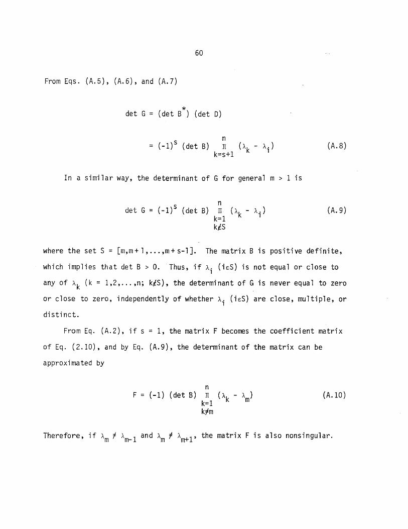
60
From Eqs. (A.5), (A.6), and (A.7)
* det G = (det B ) (det D)
= (_I)s (det B) (A.B)
In a similar way, the determinant of G for general m > 1 is
det G = (_l)s (det B) (A.9)
where the set S = [m,m+ 1 , ••• ,m+ s-lJ. The matrix B is positive definite,
which implies that det B > O. 'Thus, if Ai (isS) is not equal or close to
any of Ak (k = 1,2, ... ,n; kiS), the determinant of G is never equal to zero
or close to zero, independently of whether A. (isS) are close, multiple, or 1
distinct.
From Eq. (A.2), if s = 1, the matrix F becomes the coefficient matrix
of Eq. (2.10), and by Eq. (A.9), the determinant of the matrix can be
approxi rna ted by
n F = (-1) (det B) IT (Ak - Am)
k=1 (A.I0)
k#m
Therefore, if Am ~ Am-I and Am 1 Am+l' the matrix F is also nonsingular.

61
APPENDIX B
CONVERGENCE ANALYSIS
The convergence analysis of the methods introduced in Chapters 2 and 3
will be presented. The eigenvalue problem we deal with here is
Ax. = A. B X . (i = 1, 2 , . . . , n ) 1 1 1
(B. 1)
in which A and B are symmetric matrices of order n, and B is positive
definite. The eigenvectors x. (i ~ 1,2, ... ,n) are assumed to be ortho-1
normalized with respect to B.
B.1 Case of a Distinct Root
Let us rewrite Eq. (2.7) used for improving approximate values of a
distinct eigenvalue Aj and the corresponding eigenvector xjOf the system
represented by Eq. (B.1):
(B.2)
T - (k) B - (k) = 0 x. /),x.
J J (B.3)
where ).. (k) and 'X.(k) are approximate values of ).. and X. after k iterations, J J J J
and /),)..(k) and ~x.(k) are unknown incremental values of A.(k) and x.(k). J J J J
L~t the approximate eigenvector xj(k) and the incremental vector ~Xj(k) be expanded in a series of the true eigenvectors, i.e.,

- (k) x· J
=
n ,--,
\
L
i=l
i=l
62
(k) -c. . X. lJ 1
(k)-b.c. . x·
lJ 1
in which cij(k) and 6Cij (k) are scalar coefficients.
the vicinity of x~, - J
c .. (k)
max ~' = E: « 1 i c ..
i#j JJ
(B.4)
Since the x.(k) is in J
(B.5)
The errors in A. (k) J
and X. (k) , J
( k) and e.(k), may be defined by y. J J
A. - A.(k) J J
A. J
« 1
« 1 (B.6)
where the values of y.(k) and e.(k) are very small compared with unity. If J J
the vectors c.(k) and c~(k) are defined by J J

The e. (k) J
-*( k) and c. J
_ (k) T c. =
J
_ *( k) T c. =
J
63
(k) (k) (k) ( c 1 . ,c2 . , ... ,c. ) J J nJ
(0,0, c .. (k), 0, ... ,0) JJ
(B.7)
then represents very closely the angle between the vectors cj(k)
(s'ee Fig. 1). The task here is to estimate y. (k+l) and e. (k+l),
the e r ro r sin ~. (k - 1) and X. (k - 1 ) . J J
1 1
Let us substitute Eq. (B.4) into Eqs. (B.2) and premultiply by x. T to 1
obtain
= -
(i = 1, 2, ... ,n)
c .. lJ
(k)
(B.8)
Substitution of Eq. (B.4) into Eq. (B.3) and use of the orthonormality
of the eigenvectors with respect to B results in
n
\' c .. (k) b.c •• (k) = ° L lJ lJ
(B.9) i=l
The unknown quantities, b.A.(k) and b.C • • (k) will be found from Eqs. (B.8) J 1 J
and (B.9).
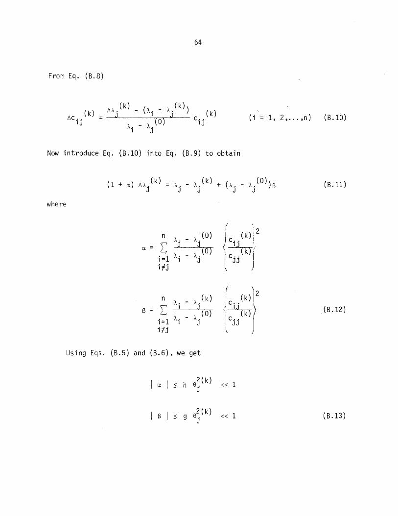
64
Frorl Eq. (B.8)
(i = 1, 2, ... ,n)
Now introduce Eq. (B .10) into Eq. (B.9) to obtain
where
n . (0) A. - A.
a = L J J A. - A.(O)
i =1 1 J i tj
Using Eqs. (B.5) and (B.6), we get
I a I
I s I
(k)!2 c. . ; lJ
( k) / c.. I JJ [
)
« 1
« 1
(B.10)
(B.11)
. (B.12)
(B.13)

where
h = max i
i~j
§ = max i
i~j
65
A. - A. (0) J J « 1
A. - A. (0) 1 J
:::: 1 (i = 1, 2, ... ,n) A. - A.(k)
1 J A. - A.(O)
1 J
Therefore, from Eq. (B. 11), the I1A. (k) J
may be approximated by
I1A.(k) = A. - A.(k) + (A. A.(O))S J J J J J
or
A . (k+ 1) = A. (k) + I1A. (k) J J J
Substitute Eq. (B.15) into Eq. (B.I0) to obtain
A. - A.(O) c .. (k) + J J (1 + S) c .. (k) lJ A. _ A.(O) lJ
1 J
(i = 1, 2, ... ,n)
(B.14)
(B.15)
(B.16)
(B.17)

66
or
(k+1) c. . = lJ
A. - A'(O) = J J (1 + S) c .. (k)
A' - A.(O) lJ 1 J
(i = 1, 2, ... ,n)
from which, it follows that
c . . ( k+ 1) = (1 + S) c.. ( k ) JJ lJ
The measure of the error in x.(k+1), e.(k+1), can now be found: J J
8. (k+ 1) J
n = \
L
i=l i]ij
n
= [ i=l i]ij
\
c .. (k+1) 2l1/2
( 1 J (k+ 1)) (
Cjj )
( ) '\ 1/2
(
Aj - A. 0 )2 (c .. (k) \ 2 ---=A .:...----A~-r-::( O~) ~ )
1 J JJ
< h 8.(k) 1
(B.18)
(B.19)
(B.20)
where h is given in Eq. (B.14) and is very small compared with unity. To
find y.(k+1), the measure of the error of A.(k+1), we use Eqs. (B.6) and J J
(B.16), giving

by which
(k+ 1) = Yj
=
<
(k+2) < Yj
67
A. - A. (k+ 1) J J
A. J
A. - A • ( 0) J J S A.
J
A· A. ( 0) e~(k) J J
9 (B.21) A. J J
A. - A.(O) J J
A. (B.22) J
Substitution of Eq. (B.20) into Eq. (B.22) and use of Eq. (B.21) results in
(k+2) y.
J = h2 y. (k+1)
J (B.23)
Hence, it can be seen from Eqs. (B.20) and (B.23) that the jth eigenvector
and eigenvalue converge linearly with errors multiplied by h (h «1) and
h2 respectively in each iteration.
B.2 Case of a Multiple Root
The convergence analysis of the method for finding a multiple eigen
value and the corresponding eigenvectors of the system given in Eq. (B.1)
will now be presented.

68
For convenience, but without loss of generality, the s low~st eigen
values are assumed to be equal, and the eigenvalue of multiplicity s is
denoted by A*, i.e., A* = Al = A2 = ... = AS' Let us rewrite Eqs. (3.21)
and (3.17), which are the basic equations for improving approximate values
of the multiple eigenvalue and corresponding eigenvectors, i.e.,
and
(~ 1 I) ,...\ \ J _. .l, '-,..., ;:, J
(j = 1, 2, ... ,s)
where Is is the unit matrix of order s, and
Y(k) = [y- (k) y- (k) y- (k)] 1 ' 2 , ... , s
-d.(k)T = (k) (k) (k) J (111j' fl2j , ... 'flsj )
(B.25)
(B.26)
(B.27)
The 11 .. (k) (j = 1, 2, ... ,s) are approximations to the multiple eigenvalue JJ
A* = Al = A2 = ••• = "s' and the Yj(k) (j = 1,2, ••• ,5) are approximations

69
- ( - (k) - (k) to the true eigenvectors x. j = 1, 2, ... ,s). The ~y. and ~d. are J J J
unknown incremental vectors for y.(k) and a.(k). J J
. Let the approximate eigenvectors y.(k) and the incremental vectors J
AYj(k) be expanded in a series of the true eigenvectors xi (i = 1, 2, ... ,n),
as in Eq. (B. 4), i. e. ,
- (k) y.
J =
n
L i=l
n
(k) -c .. X. lJ 1
- (k) ~y . = \"' ~c .. (k) X.
G lJ 1 (j = 1, 2, ... ,s)
J
Denoting the errors in
where
i=l
lJ •. JJ
(k) an d y. (k) by y. (k) J J
and
A. - lJ·· (k)
(k) = J JJ y. J A.
J
s (k) e . (k) =
j « 1
J ( k) a.
J
( s 11/2 a.(k) =! L c~.(k)~
J 1 1 J i l i =1 J
r n s/k) =) L
11/2 c~.(k) \.
1 J I
( i=s+l J
e (k) we . , J
(8.28)
have
(8.29)
(8.30)

70
The task here is to estimate the values of y.(k+1) and e.(k+1). Now J J .
let the vectors c.(k) and 6c.(k), and the matrix C(k) be J J
-c (k)T = (c (k) c (k) j 1j' 2j , ... ,
T II-c.(k) = (II (k) II (k) II (k)) U J uC1 . , uc2 · , ... , uC .
J J nJ
C(k) - [- (k) - (k) - (k)] - c1
,c2 , ... , Cs (B.31)
Then, defining the matrix X = [xl' x2' ... , X ], we may write Eq. (B.28) as n
- (k) = X c.(k) y. J J
(j = 1, 2, ... ,s) (B.32)
or
y(k) = X C(k) (B.33)
and - (k) = X 6C. (k) 6y.
J J (j = 1, 2, ... ,s) (B.34)
Substitution of Eqs. (B.32) - (B.34) into Eqs. (B.24) - (B.26), and pre
multiplication of Eq. (B.24) by XT results in
(B.35)
(B.36)
(B.37)

71
where
In = unit matrix of order n.
Let us find lICj
(k) and lId j (k) using Eqs. (B.35) - (B.37). From Eq. (B.35)
Substitution of Eq. (8.38) into Eq. (8.36) leads to
(8.39)
where
T F(k) = C(k) (A _ ~ .. (0) I )-1 C(k)
JJ n
(8.40)
Note that F(k) is a symmetric matrix of order s. Using Eq. (8.33), we can
show that
(8.41)
where
(B.42)

72
and the (l, m)th element of the symmetric matrix E(k) elm(k), is
n (0) )...* - (Co (k);
(k) ~ .. (m= 1, 2, ... ,s) e \"' JJ 1m ) = (0) \ ( k) mm L-.
).... - ~ .. i=s+1 1 JJ \ am
n )...* - ).... Ci,t(k)) c. (k) \
(k) 1 1m \
eC = (0) al( k) ! (k) ) ,m ).... i=s+1 - ~ .. am 1 JJ
(l, m = 1, 2, ... , S; l ~ m) (B.43)
The a.(k) (i = 1, 2, ... ,s) of Eq. (B.42) are defined in Eq. (B.30). By 1
Eq. (B. 29), the absol ute val ues of elm (k) (l, m = 1, 2, ... ,s) are very small
compared with unity, thus
1 (;.* _ (0)
. 2(k) 2(k) 2(k) d1 ag (a1 ' a2 ' ... ,as ) (8.44)
Similarly, the values of the s components of the vector g.(k) can be found J
fro m E q . ( 8 . 40), i. e. ,
(k) g .. JJ
( k) g .. 1J
(k) (k) a. a·
=' J * ( 0) )... - lJ·· JJ
(0) lJ .. JJ
(k) (i = llij 1, 2, ... ,s, i ~ j) (8.45)

73
where
n . (k) 2
(k) A (C . m l~ n· . = /., (0) JJ
m=s+1 Am - 11·· \ a· JJ J
n (c .(k)\(c .(k)' (k)
= - L A - A* n· . m m1 I~. (8.46) 1J . ( 0) ( k)} k i
m=s+1 Am - 11jj a. /Ia. i 1 \ J J
T Since a/ k+1) = (lll/k+l), 112/ k+1), ... , lls/k+l) by definition (see
Eq. (8.2 )), Eqs. (8.39), (8.4 ), and (8.45) result in
(k+1) ~ A* + (A* _ 11 •• (0)) (k) 11jj t-<JJ lljj (j = 1, 2, ... ,s)
(i,j =1, 2, ... ,s; i f j) (8.47)
Substitution of Eq. (8.43) into Eq. (8.38) resul ts in
s A. ( k) 1 .--. (k) (k+1 ) 1 (k) f::.C •. = (0) c..~-J C. 11 . (0) c ..
1J 1m rTlJ 1J A. - 11 .. m=1 A· - li·· 1 JJ 1 JJ
A* - Ai (k) = ---(--0-'-) C i . + ( 0 )
Ai - 11jj J Ai - lijj
(i = 1, 2, ... ,n) (8.48)

or
c .. (k+ 1) ~ 1J
A * _ (0) 11jj (k)
(0) Cij A. - 11
1 "'jj
74
(i = 1, 2, ... ,n)
from which, since A* = Al = A2 = = A ' it follows that n
Thus,
c .. (k+1) ~ c .. (k) 1J 1J
e . (k+ 1) = J
n
[ (c. \ k+ 1 ) i 2 . 1 1 J l=S+ s ~ (c. ~ k + 1 ))2 '- 1J
i=l
:5 h e.(k) J
1/2
where Y. (k) 1· S def1· ned 1· n Eq (8 30) and J . . ,
h = max i
A * (0) - lljj
A. _ (0) 1 lljj
(i = 1, 2, ... ,s)
(i = s+ 1, s+2, ... , n )
(8.49)
(8.50)
(8.51)
(8.52)
To find y.(k+1), the measure of the error of 11 .. (k+1), Eqs. (8.29) J JJ
and (8.47) are used, which results in

where n .. JJ
y. J
(k+l)
( k) i s gi ven in Eq.
In .. ( k) 12 max JJ .
1
Therefore, from Eq. (8.53)
where
z.: = max i
A. 1
Ai - fljj
From Eqs. (B.55) and (8.51),
A* -=
A* -~
(8.46).
( 0) .
75
fl .. (k+l)
JJ * A
fl .. (0)
JJ ( k) n· .
A* JJ (8.53)
Its absolute value is
2(k) z.: 8.
J
(i = s+l, s+2, ... ,n) (8.54)
(8.55)
(i = s+l, s+2, ... ,n) (8.56)
y.(k+2) = z.: 8~(k+l) J J
= h2 y. (k+ 1) J
(j = 1, 2, ... ,s) (8.57)

76
Hence, it can be seen from Eqs. (B.5n) and (8.51) that the multiple eigen-
value and the corresponding eigenvectors converge linearly with errors multi-2
plied by h (h« 1) and h respectively in each iteration.
From Eqs. (B.47) and (B.49),
lim ll .. (k) * for i j = A =
k-+oo lJ (i,j = 1, 2, ... ,s) (B. 58)
= 0 for i "1 j
and
1 i m c .. (k) = 0 k-+oo lJ
(i = S+ 1, s+2, ... , n ;
j = 1, 2, ... ,s) (8.59)
which shows that as k-+oo, the vectors x.(k) (j = 1, 2, ... ,s) span the subspace J
of Xj (j = 1, 2, ... , s) whose corresponding eigenvalue is multiple. Thus, - (k) ._ the x. (J - 1, 2, ... ,s) themselves are a set of true eigenvectors, ortho-
J
normalized with respect to 8.

77
APPENDIX C
THE BASIC THEOREMS ON THE CONSTRAINED STATIONARY-VALUE PROBLEM
Three theorems used for the development of the method for finding
multiple or close eigenvalues and the corresponding eigenvectors will be
presented. For convenience, two definitions will be given first.
Definition 1
Let S be a set of positive integers p. (i = 1,2, ... ,s) which are 1
smaller than or equal to n, the order of the matrices A and B of the
system Ax = ABx, i.e., S = (PI' P2"" ,ps). Then, R is defined as the
subspace spanned by the s eigenvectors x. (isS). 1
Definition 2
If no vector in the subspace R is orthogonal to all vectors -Yi (i = 1,2, ... ,s) (with respect to B), then the set of the vectors
Yi (i = 1,2, ... ,s) is said to be an admissible frame with respect tb the
subspace R.
Theorem 1
With the above definitions, if none of the eigenvalues A. (isS) is 1
equal to any A. (jiS), then among all admissible frames of vectors J
y. (i = 1,2, ... ,s) a frame which renders w extremum in the following con-1
strained stationary-value problem spans the subspace R, and its stationary
value is the sum of the eigenvalues A. (isS): 1

Find the stationary value of
w
subject to
-T -y .By. = 8 .. 1 J 1 J
where 8 .. is the Kronecker delta. lJ
=
78
5
L -T -y.Ay. 1 1
i=l
(i,j = 1,2, ... ,5)
Proof: For convenience, but without loss of generality, the set
S = (1,2, ... ,5 n) is taken, that ;5, R is the subspace spanned by
(C.1)
(C.2)
x. (i = 1,2, ... ,5). Let the vectors y. (i = 1,2, ... ,5) be expanded in a 1 1
series of the eigenvectors Xk (k = 1,2, ... ,n):
n
y. = L 1
(k = 1,2, ... ,n) (C.3)
k=l
It will be shown that a solution of Eqs. (C.1) and (C.2) yields
for k = 5+ 1, 5+2, •.. , n (C.5)
Sub s tit uti 0 n 0 f E q . ( C . 3 ) into Eq 5 • ( C . 1) and (C. 2) re 5 u 1 ts ; n
5 n .-- \' 2
w = L L Ak cki (C.6)
;=1 ;=1
and

n
L. cki ckj k=l
= cS •• lJ
79
(i,j = 1,2, ... ,s) (C.7)
Let us use the method of Lagrange multipliers to solve the stationary-value
problem of Eqs. (C.6) and (C.7). Introducing the undetermined multipliers
11·· (i ,j = 1,2, ... ,s) and letting 11.· = 11.·, we have the Lagrangian lJ lJ Jl
s n s s n L ~ \' 2 \ (L 8 .. ) = L L AkCki - L L 11· . Cki Ckj -
lJ lJ (C.8)
i=l k=l i=l j=l k=l
Since the first derivatives of L with respect to the unknowns ck· and 11 •. 1 1 J
should vanish,
s aL
2 ( Akc ki \"'
11 •• ck·) = a --= - L aC ki lJ J j=l
(C.9)
n aL \"' ckickj a .. = a --= -all· . L lJ lJ k=l
(C.10)
We may write Eqs. (C.9) and (C.10) in matrix form as
AC = CD (C.11)
(C.12)
where
Is = unit matrix of order s

80
and the (k,i)th element of the nxs matrix C is ck. (k = 1,2, ... ,n; 1 -
i = 1,2, ... ,s), and the (i ,j)th element of the sxs matrix D is
]1 •• (i,j = 1,2, ... ,s). Let the matrix C be partitioned into·the two lJ
submatrices C and C I where C is the sxs matrix having the elements s n-s s of the first s rows of C, and C s is the remaining (n-s)xs matrix. n-Then, Eqs. (C.11) and (C.12) may be written as
AS C = CsO s
An-s C = C 0 n-s n-s
CTC + cT C = Is s s n-s n-s
where
Since ]1 •• = ]1 •• was taken lJ Jl
by which from Eq. (C.13)
Postmul tipl ication of Eq. (C.14) by C and use of Eq. (C.17) leads to
A C CT = C OCT n-s n-s s n-s s
(C.13)
(C.14)
(C.15)
(C.16)
(C.17)
(C.18)

81
Let
u = C CT n-s s (C. 19)
Then, Eq. (C.18) yields
(i = 1,2, ... ,n-s;
j = 1,2, ... ,s) (C.20)
Since
u = C CT = 0 n-s s (C.21)
But the set of vectors y (i = 1,2, ... ,s) is an admissible frame with
respect to B, from which it is not difficult to show that
T det Cs 1- 0 (C.22)
From Eqs. (C.21) and (C.22), we obtain
C = 0 n-s (C.23)
or
(i = 1,2, ... ,s; k = s+l,s+2, ... ,n) (C.24)
This shows that the subspace spanned by the vectors Yi (i = 1,2, ... ,s) is
the subspace of the eigenvectors xi (i = 1,2, ... ,s), which is to be proved
here. Furthermore, from Eq. (C.6) we obtain
... Yetz Reference Room C1Y~1 Engineering Department
BI06 C.E. BUilding University of Illinois Urbana, Illinois 61801

82
s s ~
.---. 2 w = AkC ki L .:.._, ~.
i=l k=l
s s .-- \' 2 = L L- cki k=l ki=l
s
= L Ak k=l
which implies that the stationary value is the sum of the eigenvalues
Ak (k = 1,2, ... ,s).
Theorem 2
(C.25)
If a frame of s vectors Yi (i = 1,2, ... ,s) which are mutually ortho
normal with respect to B spans the subspace R, then Eqs. (C.13), (C.14),
and (C. 15) are satisfied, i.e., w is stationary.
Proof: Since the vectors Yi (i = 1,2, ... ,s) are in the subspace R,
and are orthonormal with respect to B,
and
or (C.26)
Hence, Eqs. (C.14) and (C.15) are satisfied. Furthermore, we have
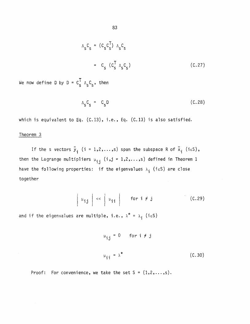
83
A C = (C CT) A C s s s s s s
= Cs
(C T A C ) s s s (C.27)
T We now define D by D = Cs AsCs ' then
A C = C 0 s s s (C.28)
which is equivalent to Eq. (C.13), i.e., Eq. (C.13) is also satisfied.
Theorem 3
-If the s vectors Yi (i = 1,2, ... ,s) span the subspace R of xi (isS),
then the Lagrange multipliers ~ .. (i,j = 1,2, ... ,s) defined in Theorem 1 lJ
have the following properties: if the eigenvalues Ai (isS) are close
together
I ~i j I « I ~i i I for i ~ j
and if the eigenvalues are multiple, i.e., A* = A' (isS) 1
~ .. = 0 1J
~ .. 11
= A*
for i f j
Proof: For convenience, we take the set S = (1,2, ... ,s).
(C.29)
(C.30)

84
Then, from Eq. (C.13)
o = CT II. C s 5 5
or
5
11· . = L AkCkiCkj lJ k=l
s s
= A L Cki
Ckj + [ ( A k - Ai) C k i C kj i k=l k=l
From Eq. (C.7)
5 r-"'"'
Ck
.C I • = o .. L, , KJ IJ
(i,j = 1,2, ... ,s)
k=l
Thus
5
11· • = [ (A - A. ) Cki Ckj lJ k 1 for i :f j
k=l
5
A. + L (A - A. ) 2 11 •• = Cki 1 1 1 k 1
k=l
If the eigenvalues A. (i = 1,2, ... ,5) are close together, i.e., 1
I Ak - A; I «Ai (k:f i), then Eq. (C.33) implies that
I 11; j I « I 11i i I for i :f j
(C.31)
(C.32)
(C.33)
(C.34)

85
Furthermore, if all the eigenvalues A. (i = 1,2, ... ,5) are multiple, i.e., 1
* A = A = A I 2 = , ... , = AS' then from Eq. (C.33)
ll· . = 0 1J
ll· . = A. = A* (i = 1,2, ... ,5) 11 1
(C.35)

86
TABLE 1. NUMBER OF OPERATIONS FOR EIGENSOLUTIONS
Method Operation
Proposed Multipl ication Method of Chapter 2
Factorization
Iterati on
Multiplication
Factorization
Solve Eq. (2.7)
Tota 1 Np
Where
Calculation Number of Operations
A-A.(O)B J
n (mb + 1)
A . (0) B t nm (m + 3) LOU = A -J a a
Ax. (k) J
n (2m + a 1)
Bx . (k) n (2mb + 1) J
r . ( k ) = Ax. ( k) _ II A . (k) B x . (k) J J J J
n
LOU = F( k) n (ma + 1)
for llX.(k) and llA.(k) J J
2n (rna + 1)
1 pn 2 (m2 + 3m + 2mb + 2) + T n a a p
(5ma
+ 2mb + 6)
[
A-L(O)B : _Bx.(k) 1 J I J
r . - ------
.f I
_x.(k) B' 0 J i .
Total number of iterations by the proposed method· Tp > Tr .
Total number of operations by the proposed method.
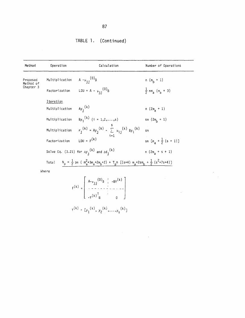
Method
Proposed Method of Chapter 3
Operation
Multiplication
Factorization
Iterati on
Multiplication
Multiplication
Multiplication
Factorization
87
TABLE 1. (Continued)
Calculation
A -fl .. (O)B JJ
LOU = A - fl .. ( 0) B JJ
Ay. (k) J
BYi(k) (i = 1,2, ..• ,s)
s r.(k) = Ay.(k) _ \' (k) B (k)
J J L flij Y i i=1
LOU = F( k)
Solve Eq. (3.21) for t:,y. (k) and ~d. (k) J J
\.Jhere
y(k) [(k) (k) (k) y 1 ,y 2 ' ... ,y s J
Number of Operations
n (mb
+ 1)
n (2ma + 1)
sn (2mb
+ 1)
sn
sn [rna + t (s + I)J
n (2m + s + 1) a

Method
Robi nson-Ha rri s Method
88
TABLE 1. (Continued)
Operati on Calculation
Multiplication A-L(k)B J
r. (k) = Multiplication J
(A - >..(k)B) x.(k) J J
Multiplication Bx. (k) J
Factorization LOU = G(k)
Solve Eq. (2.6) for lIx.(k) and lI>..(k) J J
Total
Hhere
A-.\ . (k) B J
G(k)
(k) T -x· B
J
: I
I
N r
-Bx . (k) J
0
Number of Operations
n (m + a 1 )
n (m + a 1)
n (mb + 1 )
i nm (m + 5) a a
2n (m + 1) a
+ n
Tr = Total number of iterations by the Robinson-Harris method. Tr < Tp.
Nr = Total number of operations by the Robinson-Harris method.

89
TABLE 1. (Conti nued)
Method Opera ti on Calculation Number of Operations
Subspace Factorization LOU = A nma (m + 3)/2 a Iteration Method
Iteration
Multiplication BX(k-1)
Solve for y(k) Ay(k) = BX(k-1)
Multiplication A*(k) = y(k)TBX (k-1)
Mu 1t i p 1 i cat ion By(k)
Multiplication B*(k) = y(k)TBy(k)
Sol ve for Z(k) A*(k)Z(k) = B*(k)Z(k)O(k)
and O(k)
Multiplication
Subtota 1
qn (2mb + 1)
qn (2ma + 1)
qn (q + 1)/2
qn (2mb + 1)
qn (q + 1)/2
3 a (q ) neglected
2 nq
qn (2ma + 4mb + 2q + 4)
Sturm Seguence Check
Multiplication
Factorization
Total
A- A (k) B p
LOU = A- /.. (k) B p
n (mb
+ 1)
T qn (2m) + 4 b + 2q + 4) + n (m2 + 3ma + mb + 1) sam a
Note: q max (2p. p+8)
Ts Total number of iterations by subspace iteration method.
NS Total number of ooerations by subspace iteration method.
It is assumed that ma : mb.

90
TABLE 2. EIGENVALUES OF THE PLANE FRAME PROBLEM (DISTINCT ROOTS)
Method of
Analysis
Proposed Method
Robinson Harris Method
*
Iteration Eigenvalues
Number (1) (2) (3)
0 0.474744xlOO 0.443880xl01 0.132953xl02
(0.36xlO-2)* -1 (0.28xlO ) (0. 77xlO-1)
0.474744xlOO 0.443876xl01 0.132921xI02
-5 (0.44xlO ) -3 (0.45xlO ) -2 (0.38xlO )
2 0.474744xlOO 0.443876xlQl 0.132921xl02
(O.82xlO- 13) -9 (O.27xlO ) -6 (O.17xlO )
3
4
0 O.474744x100 0.443880xlO 1 0.132953xl02 -2 (0.36xlO ) (O.28xlO- 1) (0.77xlO- 1)
1 O.474744xlOO 0.443876xl01 0.13292lxl02 -5 (0.44xlO ) -3 (0.45xlO ) -2 (0.38xlO )
2 0.474744xlOO 0.443876xl01 O.132921xl02
(0.82xlO- 13 ) -9 (0.27xlO ) -6 (0.17x10 )
3
Numbers in parentheses indicate errors in the approximate eigenvectors x.(k).
J
(4)
0.284745xl02
0 (0.22xlO )
0.284091xl02
-1 (0.27x10 )
0.284091xlO2
-3 (0 .18x 10 )
0.284091xl02
-5 (0.19xlO )
O. 284091x 102 -7 (0.23xlO )
O.284745xl02
(0.22xlO a
0.284091xl02
-1 (0.27xlO )
0.284091xl02
-3 (0.18xlO )
0.284091xl02
( -8 0.13xlO )
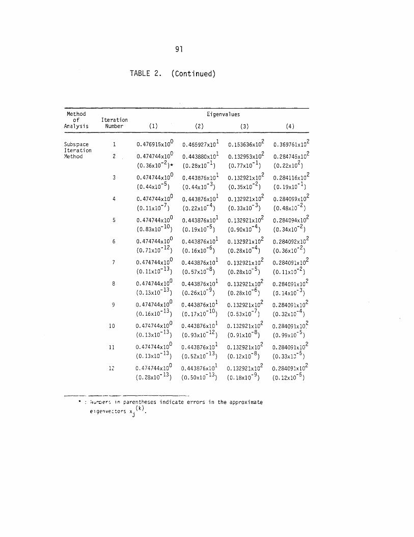
91
TABLE 2. (Continued)
Method Eigenvalues of Iteration
Analysis Number (1) (2 ) (3) (4 )
Subspace 1 0.476915x100 0.465927x101 0.153636x10² 0.369761x10² Iteration
0.474744x100 0.443880x101 0.132953x10² 0.284745x10² Method 2
(0.36xlO-2)* -1 (0.28x10 ) -1 (0.77x10 ) 2 (0.22xlO )
3 0.474744x100 O.443876x101 0.132921x10² 0.284116x10²
-5 (O.44x10 ) -3 (0.44x10 ) -2 (0.35xlO ) -1 (0.19xlO )
4 0.474744x100 0.443876x101 0.132921x10² 0.284099x10²
-7 (0.llx10 ) -4 (0.22x10 ) -3 (O.33x10 ) -2 (0.48xlO )
5 0.474744x100 0.443876x101 0.132921x10² 0.284094xl02
(0.83x10- 1O ) -5 (0.19x10 ) -4 (0.90xlO ) -2 (0.34xlO )
6 0.474744xlOO 0.443876xlOl 0.132921xlO2 0.284092x10²
(0.71xlO- 12 ) -6 (0.16xlO ) -4 (0.28xlO ) -2 (0.36xlO )
7 0.474744xlOO 0.443876x101 0.132921xl02 0.284091xl02
(O.llxlO- 13 ) -8 (O.57xlO ) -5 (0.28xlO ) -2 (O.llxlO )
8 O.474744xlOO 0.443876x101 0.132921xl02 0.284091xl02
(O.13xlO- 13 ) -9 (0.26xlO ) -6 (0.28xlO ) -3 (0.14xlO )
9 0.474744xlOO 0.443876xlO l 0.132921x10² 0.284091x10²
(0.16XlO- 13 ) (0.17x10- 10 ) -7 (0.53xlO ) -4 (0.32xlO )
10 0.474744xlOO 0.443876xlO l 0.132921xl02 0.284091xl0 2
(0. 13xlO- 13 ) (0.93xIO- 12 ) -8 (0.91xlO ) -5 (0.99xlO )
11 0.474744xlOO 0.443876xlO l 0.132921xl02 0.284091xl02
(0.13x10- 13 ) (0.52xl0- 13 ) -8 (0.12xlO ) -5 (0.33xlO )
12 0.474744xlOO O.443876xlOl O.132921xlO2 O.284091xlO2
(O.28xlO- 13 ) (O.50xl0- 13 ) -9 (O.18xlO ) -5 (0.12xlO )
-----* :wnDers 1 n parentheses i nd i ca te errors in the approximate
floenvectors x.(k). - J

92
TABLE 3. EIGENVALUES OF THE CIRCULAR ARCH PROBLEM (DISTINCT ROOTS)
Method Eigenvalues/AO* of Iteration
Analysis Number (1) (2 ) (3)
Proposed 0 O.102714xlO-2 0.9l95l6xlO- 2 O.363073xlO- l
Method 0.102640xlO- 2 0.909467xlO-2 O.34l422xlO- l 1 (O.59xlO- 3)** -2 (O.53xlO ) -1 (O.35xlO )
2 O.102640xlO- 2 0.909467xlO-2 O.34l448xlO- l -8 (0.26xlO ) -5 (O.lOxlO ) -3 (O.2lxlO )
3 0.909467xlO- 2 O.34l448xlO- l
(O:lOxlO-8) -5 (O.17xlO )
4 O.34l448xlO- l -7 (O.33xlO )
Robinson- 0 O.102714xlO-2 0.9l95l6xlO-2 O.363073xlO- l
Harris O.102640xlO-2 O.909467xlO- 2 O.34l422xlO- l Method 1
-3 (O.59xlO ) -2 (0.53xlO ) -1 (0.35xlO )
2 0.102640xlO-2 0.909467xlO-2 O.34l448xlO- l
-8 (0.26xlO ) -5 (O.lOxlO ) -3 (O.2lx10 ).
3 0.909467x10⁻² O.341448x10 -1
(0. 45xlO- 12 ) -8 (0.20x10 )
2 2 * . AO = E/pa (1-\1 ).
** Numbers in parentheses indicate errors in the approximate eigenvectors x.(k).
J

93
TABLE 3. (Continued)
Method Ei genva 1 ues/ AO * of Itera ti on
Ana lysi s Number ( 1) (2) (3)
Subspace 0.102714x10- 2 0.919516x10- 2 0.363073x10- 1
Iterat; on 0.102640x10- 2 0.909468x10- 2 0.341476x10- 1 Method 2 (0.59x10- 3)** -2 (0.52x10 ) -1 (0.32x10 )
3 0.102640x10- 2 0.909467x10- 2 0.341448x10- 1
-6 (0.41x10 ) -4 (0.62x10 ) -2 (0.26x10 )
4 0.102640x10⁻² 0.909467x10⁻² 0.341448x10- 1
(0. 58xlO- 9) -5 (0.12x10 ) -3 (0.23x10 )
5 O.102640X10- 2 0.909467x10⁻² 0.341448x10- 1
(0.12xlO- ll ) -7 (O.28xlO ) -4 (0.21x10 )
6 0.102640xlO-2 0.909467x1O- 2 0.341448x10- 1
(0.23x10- 13 ) -9 (0.79xlO ) -5 (0.19xlO )
7 0.102640x10⁻² 0.909467x10- 2 0.341448x10- 1
(0. 12x10- 13 ) (0.25xlO- 10 ) -6 (O.17xlO )
2 2 * . AO = E/pa (I-v).
** Numbers in parentheses indicate errors in the approximate
eigenvectors xj(k).

94
TABLE 4. EIGENVALUES OF THE SQUARE PLATE PROBLEM (DOUBLE ROOTS)
Method Eigenvalues/a* of Iteration
Analysis Number (I) (2 ) (3)
Proposed 0 O.375840x1O I O.2302I2x102 O.2302I2x102 Method
O.375838xlO l O.230I2lx102 O.230I2lxlO2
(O.80xlO- 3)** (O.lOXlO- l ) -1 (O.lOxlO )
2 O.375838xlOl O.230I2lxlO2 O.230l2lxlO2
( O. 44 xl 0 -11 ) (O.46xIO- 7) (O.46xlO- 7)
Subspace O.375840xlO l O.2302l2xlO2 O.2302l2xlO2 Iteration
O.375838xlOl O.230I2lxlO2 O.230l2lxlO2 Method 2 (O.80XIO- 3) (O.lOxIO- l ) (O.IOXIO- I )
3 O.375838xlO l O.230l21xlO2 O.230l2lx102 -6 (O.65xlO ) (O.l1XIO- 3) (O.llxlO- 3)
4 O.375838xlOl O.230l2lxlO2 O.230l21xlO2
(O.53xlO- 9) -5 (O.13xIO ) -5 (O.13xIO )
5 O.375838xlO l O.230I2lxlO2 O.230l21xlO2
(O.44xIO- 12 ) -7 (O.15xlO ) -7 (O.15xlO )
.. :l = n40 /(a4
p). where 0 = Eh 3/12(1 - }). e e
~umbers in parentheses indicate errors in the approximate e1genvectors Yj(k).
(4)
O.530627xlO2
O.529932xlO2 -1 (O.2lxlO )
O.529932xlO2 -6 (O.59xlO )
O.530627xlO2
O.529932xlO2
-1 (O.2IxlO )
O.529932x102
-3 (O.43xlO )
O.529932xlO2 -5 (O.90xlO )
O.529932xlO2 -6 (O.19xlO )

95
TABLE 5. EIGENVALUES OF THE RECTANGULAR PLATE PROBLEM (CLOSE ROOTS)
Method Eigenvalues/o.* of Iteration
Analysis Number (1) (2 ) (3)
Proposed 0 0.368470x101 O.222957xl02 0.228454xl02
Method 0.268468x101 O.222868xl02 0.228264x10²
-3 (0.80xlO ) -1 (O.lOxlO ) (O.IOxlO- I )
2 0.368468x10 1 0.222868x10² 0.228364xl02
(0.44xlO- ll ) -7 (0.47xlO ) -7 (O.45xlO )
Subspace 0.368470x1Ol O.222957xl02 0.228454x10²
Iteration 0.368468x1O l 0.222868xl02 O.228364x102 Method 2
-3 (0.80xlO ) -1 (O.lOxlO ) -1 (O.lOxIO )
3 0.368468xlO I 0.222868x10² 0.228364xl02
-6 (0.65xI0 ) -3 (O.llxlO ) -3 (O.llxIO )
4 0.368468x1O l 0.222868xl02 0.228364xl02
-9 (0.53xlO ) -5 (O.13xIO ) -5 (O.13xlO )
5 O.368468x1Ol 0.222868xlO2 O.228364x102
(0.46xlO- 12 ) -7 (0.15xlO ) -7 (0.14xlO )
':r ii 4 ) 0 - h3/ 2( 2) - - e ,a " ,w~ere e - Ell - \! •
r,urtJers In parentheses indicate errors in the approximate
elqenvectors y.(k). - J
(4)
O.520215x102
O.519522x102
-1 (0.2lxlO )
O.5l9533x102
-6 (0.59xlO )
0.5202l5x102
O.5l9533xlO2
-1 (0.2lxlO )
O.5l9533xl02
-3 (0.43xlO )
0.519533x10²
(O.90xlO -5)
O.5l9533xlO2
-6 (O.19xI0 )

96
TABLE 6. COMPARISON OF THE TOTAL NUMBER OF OPERATIONS
Input Data NLmber of Number of Operations Ratio Problem I terati ons
Type n rna mb p q T T T N N Ns Nr/Np N/Np p r s p r
Frame 330 35 35 4 10 10 9 12 3.50xl06 4.57xl06 9.72xl06 1. 31 2.78
Arch 22 4 o 3 5 9 8 7 8.87xl03 9.77xl03 1. 76xl04 1.10 1. 98
Plate 39 16 16 4 9 8 5 1. 27xl05 2.20xl05 1. 73
Note
n Order of stiffness and mass matrices
rna Average half bandwidth of stiffness matrix
mb Average half bandwidth of mass matrix
p Number of eigenvalues and eigenvectors sought
q Number of iteration vectors, q = max (2p, p+8)
Tp Number of iterations by the proposed method
Tr Number of iterations by the Robinson-Harris method
Ts Number of iterations by the subspace iteration method
N Total number of operations by the proposed method p
N Total number of operations by the Robinson-Harris method r
Ns Total number of operations by the subspace iteration method

97
TABLE 7. COMPARISON BETWEEN THE THEORETICAL CONVERGENCE RATES FOR EIGENVECTORS AND THE NUMERICAL RESULTS - FRAME PROBLEM
(DISTINCT ROOTS)
Method Eigenvalue Number of I tera ti on
Analysis Number 2 3 4
Proposed 1 1. 9x10 -8 6.0x10 -7 4.4x10 -5 6.7xlO -3
Method 2 1.1xlO -2
3 1.2x10⁻²
Theory 1. 3xlO-8 1. Ox10 -5 3.6x10⁻⁴ 1. 2x10 -2
Subspace 2 1.2x10 -3 1. 6xlO -2 4.5xlO -2 8.6xlO -2
Iteration 3 2.5xlO- 3 5.0xlO- 2 -2 -1 Method 9.4xlO 2.5xlO
7.5xlO- 3 8.7xlO-2 -1 7.1xlO- 1 4 2.7xl0
5 8.6xl0- 3 8.4xlO -2 3.1xlO- 1 1. Ix 10 -0
6 1. 5xl0- 3 3.6xl0 -2 1. Oxl0- 1 3.1x10 -1
7 * 4.6xl0-2 1. Ox10- 1 1.3xl0 -1
6.5xlO- 2 1 -1 8 * 1.9xI0-.L 2.3xl0
9 * 5.5xl0- 2 1. 7xl0- 1 3.1xl0 -1
10 * 5.6xl0 -2 1.3xl0- 1 3.3xl0 -1
11 * * 1.5xlO- 1 3.6xlO -1
Theory 5.6xl0 -3 5.2xl0 -2 1.6xlO- 1 3.3xl0 -1
* Errors too small for comparison because of round-off error.

98
TABLE 8. COMPARISON BETWEEN THE THEORETICAL CONVERGENCE RATES FOR EIGENVECTORS AND THE NUMERICAL RESULTS - SQUARE PLATE PROBLEM
(DOUBLE ROOTS)
Method Eigenvalue Number of Iteration
Analysis Number 1 2 3 4
Proposed 1 5.5xlO -9 4.6xlO -6 4.6xlO -6 2.8x1O -5
Method Theory 1. Ox 10 -6 4.7x1O -4 4.7x1O-4 2.3x1O -3
Subspace 2 8.1x1O-4 1.lx1O -2 1.1x1O -2 2.0x1O -2 Iteration 3 -4 -2 1. 2x1O-2 -2 Method 8.2x1O 1. 2x1O 2.1x1O
-4 1. 2x1O-2 -2 -2 4 8.3x1O 1. 2x1O 2.1x1O Theory 1.1xlO -2 6.8xlO --2 . -2
6.8x1O 1. 6x1O -1

99
TABLE 9. NUMERICAL CONVERGENCE RATES FOR EIGENVECTORS -RECTANGULAR PLATE PROBLEM
(CLOSE ROOTS)
Method Eigenvalue Number of Itera ti on
Ana 1ys i s Number 2 3 4
Proposed 5.5x1O -9 4.7x1O -6 4.5x1O -6 2.8x1O Method
'Subspace 2 8.1x1O -4 1. 1xlO -2 1.lxlO -2 2.0x1O Iteration -4 -2 -2 Method 3 8.2x1O 1.2xlO 1. 2x1O 2.1x1O
-4 -2 -2 4 8.7x1O 1. 2x1O 1.lxlO 2.1x1O
Theory 1.1x1O -2 6.8x1O- 2 7.0x1O -2 1. 6x1O
-5
-2
-2
-2
-1

100
~=====-----------------------------~Xj
~~~~--------~+-----------------~Cj e ~ k+1) J
FIG. 1 ESTIMATION OF ERRORS IN APPROXIMATE EIGENVECTORS

101
/77T 7'''77 777r 77'?7 77 77.'17 "~ 7777- )'7."7
10 at 6.1 m = 61.0 m
For All Beams and Columns Area of Cross-Section
Moment of Inertia of Cross-Section Young's Modulus
Mass Density
A = 2.787xlO- l m2
I = 8.631xlO-3 m4
E = 2.068xl010 Pa
p = 1.602xl04 kg/m3
FIG. 2 TEN-STORY, TEN-BAY PLANE FRAME
77. ~ )7.~
E LO o r()
II
E LO Q r()


DISTRIBUTION LIST
for
UNCLASSIFIED TECHNICAL REPORTS
474:NP:7l6:lab 78u474-6l9
ONR Code 474 May 1980
The ONR Structural Mechanics Contract Research Program
Notes:
This list consists of:
Part 1 - Government Activities Part 2 - Contractors and Other
Technical Collaborators
Except as otherwise indicated, forward one CODY of all Unclassified Technical Reports to each of the addressees listed herein.
Where more than one attention addressee ~s
indicated, the individual copies of the report should be mailed separately.

Part 1 - Government Administrative and Liaison Activities
Office of Naval Research Department of the Navy Arlington, Virginia 22217 Attn: Code 474 (2)
Code 471 Code 200
Director Office of Naval Research
Eastern/Central Regional Office 666 Summer Street Boston, Massachusetts 02210
Director Office of Naval Research
Branch. Office 536 South Clark Street Chicago; Illinois 60605
Director Office of Naval Research New York Area Office 715 Broadway - 5th Floor New York, New York 10003
Director Office of Naval Research
Western Regional Office 1030 East Green Street Pasadena, California 91106
Naval Research Laboratory (6) Code 2627 Washington, D.C. 20375
Defense Technical Information Center (12) Cameron Stat ion Alexandria, Virginia 22314
Undersea Explosion Research Division Naval Ship Research and Development
Center Norfolk Naval Shipyard Portsmouth, Virginia 23709 Attn: Dr. E. Palmer, Code 177
Navy (Con't.)
474:NP:7l6:lab 78u474-6l9
Naval Research Laboratory Washington, D.C. 20375 Attn: Code 8400
8410 8430 8440 6300' 6390 6380
David W. Taylor Naval Ship Research and Development Center
Annapolis, Maryland 21402 Attn: Code 2740
28 281
Naval Weapons Center China Lake, California 93555 Attn: Code 4062
4520
Commanding Officer Naval Civil Engineering Laboratory Code L3l Port Hueneme, California 93041
Naval Surface Weapons Center White Oak Silver Spring, Maryland 20910 Attn: Code R-10
G-402 K-82
Technical Director Naval Ocean Systems Center San Diego, California 92152
Supervisor of Shipbuilding U.S. Navy Newport News, Virginia 23607
Navy Underwater Sound Reference Division
Naval Research Laboratory P.O. Box 8337 Orlando, Florida 32806
Chief of Naval Operations Department of the Navy Washington, D.C. 20350 Attn: Code OP-098
Navy (Con't.)
Strategic Systems Project Office Department of the Navy Washington, D.C. 20376 Attn: NSP-200
Naval Air Systems Command Department of the Navy Washington, D.C. 20361 Attn: Code 5302 (Aerospace and Structures)
604 (Technical Library) 320B (Structures)
Naval Air Development Center Warminster, Pennsylvania 18974 Attn: Aerospace Mechanics
Code 606
u.S. Naval Academy Engineering Department Annapolis, Maryland 21402
Naval Facilities Engineering Command 200 Stovall Street Alexandria, Virginia 22332 Attn: Code 03 (Research and Development)
04B 045
14114 (Technical Library)
Naval Sea Systems Command Department of the Navy Washington, D.C. 20362 Attn: Code 05H
312 322 323 05R 32R
474:NP:7l6:lab 78u474-6l9
Navy (Con' t.)
Commander and Director David W. Taylor Naval Ship
Research and Development Center Bethesda, Maryland 20084 At tn: Code 042
17 172 173 174
1800 1844
012.2 1900 1901 1945 1960 1962
Naval Underwater Systems Center Newport, Rhode Island 02840 Attn: Bruce Sandman, Code 3634
Naval Surface Weapons Center Dahlgren Laboratory Dahlgren, Virginia 22448 Attn: Code G04
G20
Technical Director Mare Island Naval Shipyard Vallejo, California 94592
U.S. Naval Postgraduate School Library Code 0384 Monterey, California 93940
Webb Institute of Naval Architecture Attn: Librarian Crescent Beach Road, Glen Cove Long Island, New York 11542
Commanding Officer (2) U.S. Army Research Office P • o. Bo x 12211 Research Triangle Park, NC 27709 Attn: Mr. J. J. Murray, CRD-AA-IP
Army (Con't.)
Watervliet Arsenal MAGGS Research Center Watervliet, New York 12189 Attn: Director of Research
u.s. Army Materials and Mechanics Research Center
Watertown, Massachusetts 02172 Attn: Dr. R. Shea, DRXMR-T
u.s. Army Missile Research and Development Center
Redstone Scientific Information Center
Chief, Document Section Redstone Arsenal, Alabama 35809
Army Research and Development Center
Fort Belvoir, Virginia 22060
NASA
National Aeronautics and Space Administration
Structures Research Division Langley Research Center Langley Station Hampton, Virginia 23365
National Aeronautics.and Space Administration
Associate Administrator for Advanced Research and Technology
Washington, D.C. 20546
Air Force
Wright-Patterson Air Force Base Dayton, Ohio 45433 Attn: AFFDL (FB)
( FBR) ( FBE) ( FBS)
AFML (HBM)
Chief Applied Mechanics Group U.S. Air Force Institute of Technology Wright-Patterson Air Force Base Dayton, Ohio 45433
474:NP:7l6:lab 78u474-6l9
Air Force (Con't.)
Chief, Civil Engineering Branch WLRC, Research Division Air Force Weapons Lab-oratory Kirtland Air Force Base Albuquerque, New Mexico 87117
Air Force Office of Scientific Research Bolling Air Force Base Washington, D.C. 20332 Attn: Mechanics Division
Department of the Air Force Air University Library Maxwell Air Force Base Montgomery, Alabama 36112
Other Government Activities
Commanda.nt Chief, Testing and Development Division U.S. Coast Guard 1300 E Street, NW. Washington, D.C. 20226
Technical Director Marine Corps Development
and Education Command Quantico, Virginia 22134
Director Defense Research and Engineering
Technical Library Room 3C128 The Pentagon Washington, D.C. 20301
Dr. M. Gaus National Science Foundation Environmental Research Division Washington, D.C. 20550
Library of Congress Science and Technology Division Washington, D.C. 20540
Director Defense Nuclear Agency Washington, D.C. 20305 Attn: SPSS

Other Government Activities (Con't)
Mr. Jerome Persh Staff Specialist for Materials
and Structures OUSDR&E, The Pentagon Room 3D1089 Washington, D.C. 20301
Chief, Airframe and Equipment Branch FS-120 Office of Flight Standards Federal Aviation Agency Washington, D.C. 20553
National Academy of Sciences National Research Council Ship Hull Research Committee 2101 Constitution Avenue Washington, D.C. 20418 Attn: Mr. A. R. Lytle
National Science Foundation Engineering Mechanics Section Division of Engineering Washington, D.C. 20550
Picatinny Arsenal Plastics Technical Evaluation Center Attn: Technical Information Section Dover, New Jersey 07801
Maritime Administration Office of Maritime Technology 14th and Constitution Avenue, NW. Washington, D.C. 20230
PART 2 - Contractors and Other Technical Collaborators
Universities
Dr. J. Tinsley Oden University of Texas at Austin 345 Engineering Science Building Austin, Texas 78712
Professor Julius Miklowitz California Institute of Technology Division of Engineering
and Applied Sciences Pasadena, California 91109
474:NP:7l6:lab 78u474-6l9
Universities (Con't)
Dr. Harold Liebowitz, Dean School of Engineering and
Applied Science George Washington University Washington, D.C. 20052
Professor Eli Sternberg California Institute of Technology Division of Engineering and
Applied Sciences Pasadena, California 91109
Professor Paul M. Naghdi University of California Department of Mechanical Engineering Berkeley, California 94720
Professor A. J. Dure11i Oakland University School of Engineering Rochester, Missouri 48063
Professor F. L. DL~aggio Columbia University Department of Civil Engineering New York, New York 10027
Professor Norman Jones The University of Liverpool Department of Mechanical Engineering P. O. Box 147 Brownlow Hill Liverpool L69 3BX England
Professor E. J. Skudrzyk Pennsylvania State University Applied Research Laboratory Department of Physics State College, Pennsylvania 16801
Professor J. Klosner Polytechnic Institute of New York Department of Mechanical and
Aerospace Engineering 333 Jay Street Brooklyn, New York 11201
Professor R. A. Schapery Texas A&M University Department of Civil Engineering College Station, Texas 77843

Universities (Con't.)
Professor Walter D. Pilkey University of Virginia Research Laboratories for the
Engineering Sciences and Applied Sciences
Charlottesville, Virginia 22901
Professor K. D. Willmert Clarkson College of Technology Department of Mechanical Engineering Potsdam, New York 13676
Dr. Walter E. Haisler Texas A&M University Aerospace Engineering Department College Station, Texas 77843
Dr. Hussein A. Kamel University of Arizona Department of Aerospace and
Mechanical Engineering Tucson, Arizona 85721
Dr. S. J. Fenves Carnegie-Mellon University Department of Civil Engineering Schenley Park Pittsburgh, Pennsylvania 15213
Dr. Ronald L. Huston Department of Engineering Analysis University of Cincinnati Cincinnati, Ohio 45221
Professor G. C. M. Sih Lehigh University Institute of Fracture and
Solid Mechanics Bethlehem, Pennsylvania 18015
Professor Albert S. Kobayashi University of Washington Department of Mechanical Engineering Seattle, Washington 98105
Professor Daniel Frederick Virginia Polytechnic Institute and
Department of Engineering Mechanics Blacksburg, Virginia 24061
474:NP:7l6:lab 78u474-6l9
Universities (Con't)
Professor A. C. Eringen Princeton University Department of Aerospace and
Mechanical Sciences Princeton, New Jersey 08540
Professor E. H. Lee Stanford University Division of Engineering Mechanics Stanford, California 94305
Professor Albert I. King Wayne State University Biomechanics Research Center Detroit, Michigan 48202
Dr. V. R. Hodgson Wayne State University School of Medicine Detroit, Michigan 48202
Dean B. A. Boley Northwestern University Department of Civil Engineering Evanston, Illinois 60201
Professor P. G. Hodge, Jr. University of Minnesota Department of Aerospace Engineering
and Mechanics Minneapolis, Minnesota 55455
Dr. D. C. Drucker University of Illinois Dean of Engineering Urbana, Illinois 61801
Professor N. M. Newmark University of Illinois Department of Civil Engineering Urbana, Illinois 61803
Professor E. Reissner University of California, San Diego Department of Applied Mechanics La Jolla, California 92037
Professor William A. Nash University of Massachusetts Department of Mechanics and
Aerospace Engineering Amherst, Massachusetts 01002

Universities (Con't)
Professor G. Herrmann Stanford University Department of Applied Mechanics Stanford, California 94305
Professor J. D. Achenbach Northwest University Department of Civil Engineering Evanston, Illinois 60201
Professor S. B. Dong University of California Department of Mechanics Los Angeles, California 90024
Professor Burt Paul University of Pennsylvania Towne School of Civil and
Mechanical Engineering Philadelphia, Pennsylvania 19104
Professor H. W. Liu Syracuse University Department of Chemical Engineering
and Metallurgy Syracuse, New York 13210
Professor S. Bodner Technion R&D Foundation Haifa, Israel
Professor Werner Goldsmith University of California Department of ~echanical Engineering Berkeley, California 94720
Professor R. S. Riv1in Lehigh University Center for the Application
of Mathematics Bethlehem, Pennsylvania 18015
Professor F, A. Cozzarelli State University of New York at
Buffalo Division of Interdisciplinary Studies Karr Parker Engineering Building Chemis~ry Road Buffalo, New York 14214
474:NP:7l6:lab 78u474-6l9
Universities (Con't)
Professor Joseph L. Rose Drexel University Department of Mechanical Engineering
and Mechanics Philadelphia, Pennsylvania 19104
Professor B. K. Donaldson University of Maryland Aerospace Engineering Department College Park, Maryland 20742
Professor Joseph A. Clark Catholic University of America Department of Mechanical Engineering Washington, D.C. 20064
Dr. Samuel B. Batdorf University of California School of Engineering
and Applied Science Los Angeles, California 90024
Professor Isaac Fried Boston University Department of Mathematics Boston, Massachusetts 02215
Professor E. Krempl Rensselaer Polytechnic Institute Division of Engineering Engineering Mechanics Troy, New York 12181
Dr. Jack R. Vinson University of Delaware Department of Mechanical and Aerospace
Engineering and the Center for Composite Materials
Newark, Delaware 19711
Dr. J. Duffy Brown University Division of Engineering Providence, Rhode Island 02912
Dr. J. L. Swedlow Carnegie-Mellon University Department of Mechanical Engineering Pittsburgh, Pennsylvania 15213

Universities (Con't)
Dr. V. K. Varadan Ohio State University Research Foundation Department of Engineering Mechanics Columbus, Ohio 43210
Dr. Z. Hashin University of Pennsylvania Department of Metallurgy and
Materials Science College of Engineering and
Applied Science Philadelphia, Pennsylvania 19104
Dr. Jackson C. S. Yang University of Maryland Department of Mechanical Engineering College Park, Maryland 20742
Professor T. Y. Chang University of Akron Department of Civil Engineering Akron, ohio 44325
Professor Charles W. Bert University of Oklahoma School of Aerospace, Mechanical,
and Nuclear Engineering Norman, Oklahoma 73019
Professor Satya N. Atluri Georgia Institute of Technology School of Engineering and
Mechanics Atlanta, Georgia 30332
Professor Graham F. Carey University of Texas at Austin Department of Aerospace Engineering
and Engineering Mechanics Austin, Texas 78712
Dr. S. S. Wang University of Illinois De?artment of Theoretical and
Applied Mechanics Urbana, Illinois 61801
Professor J. F. Abel Cornell University Department of Theoretical
and Applied Mechanics Ithaca, New York 14853
474:NP:7l6:1ab 78u474-6l9
Universities (Con't)
Professor V. H. ~eubert
Pennsylvania State University Department of Engineering Science
and Mechanics . University Park, Pennsylvania 16802
Professor A. W. Leissa Ohio State University Department of Engineering Mechanics Columbus, Ohio 43212
Professor C. A. Brebbia University of California, Irvine Department of Civil Engineering School of Engineering Irvine, California 92717
Dr. George T. ~ahn Vanderbilt University Mechanical Engineering and
Materials Science Nashville, Tennessee 37235
Dean Richard H. Gallagher University of Arizona College of Engineering Tucson, Arizona 85721
Professor E. F. Rybicki The University of Tulsa Department of Mechanical Engineering Tulsa, Oklahoma 74104
Dr. R. Haftka Illinois Institute of Technology Department of Mechanics and Mechanical
and Aerospace Engineering Chicago, Illinois 60616
Professor J. G. de Oliveira Massachusetts Institute of Technology Department of Ocean Engineering 77 Massachusetts Avenue Cambridge, Massachusetts 02139
Dr. Bernard W. Shaffer Polytechnic Institute of New York Route 110 Farmingdale, New York 11735
Industry and Research Institutes
Dr. Norman Hobbs Kaman AviDyne Division of Kaman
Sciences Corporation Burlington, Massachusetts 01803
Argonne National Laboratory Library Services Department 9700 South Cass Avenue Argonne, Illinois 60440
Dr. M. C. Junger Cambridge Acoustical Associates 54 Rindge Avenue Extension Cambridge, Massachusetts 02140
Mr. J. H. Torrance General Dynamics Corporation Electric Boat Division Groton, Connecticut 06340
Dr. J. E. Greenspon J. G. Engineering Research Associates 3831 Menlo Drive Baltimore, Maryland 21215
Newport News Shipbuilding and Dry Dock Company
Library Newport News, Virginia 23607
Dr. W. F. Bozich McDonnell Douglas Corporation 5301 Bolsa Avenue Huntington Beach, California
Dr. H. N. Abramson Southwest Research Institute 8500 Culebra Road San Antonio, Texas 78284
Dr. R. C. DeHart Southwest Research Institute 8500 Culebra Road San Antonio, Texas 78284
Dr. M. L. Baron Weidlinger Associates 110 East 59th Street New York, New York 10022
92647
474:NP:7l6:lab 78u474-6l9
Industry and Research Institutes (Con't)
Dr. T. L. Geers Lockheed Missiles and Space Company 3251 Hanover Street Palo Alto, California 94304
Mr. William Caywood Applied Physics Laboratory Johns Hopkins Road Laurel, Maryland 20810
Dr. Robert E. Dunham Pacifica Technology P.O. Box 148 Del Mar, California 92014
Dr. M. F. Kanninen Battelle Columbus Laboratories 505 King Avenue Columbus, Ohio 43201
Dr. A. A. Hochrein Daedalean Associates, Inc. Springlake Research Road 15110 Frederick Road Woodbine, Maryland 21797
Dr. James W. Jones Swanson Service Corporation P.O. Box 5415 Huntington Beach, California 92646
Dr. Robert E. Nickell Applied Science and Technology 3344 North Torrey Pines Court Suite 220 La Jolla, California 92037
Dr. Kevin Thomas Westinghouse Electric Corp. Advanced Reactors Division P. O. Box 158 Madison, Pennsylvania 15663
Dr. H. D. Hibbitt Hibbitt & Karlsson, Inc. 132 George M. Cohan Boulevard Providence, Rhode Island 02903
Dr. R. D. Mindlin 89 Deer Hill Drive Ridgefield, Connecticut 06877

Industry and Research Institutes (Conrt)
Dr. Richard E. Dame Mega Engineering 11961 Tech Road Silver Spring, Maryland 20904
Mr. G. M. Stanley Lockheed Palo Alto Research
Laboratory 3251 Hanover Street Palo Alto, California 94304
Mr. R. L. Cloud Robert L. Cloud Associates, Inc. 2972 Adeline Street Berkeley, California 94703
474:NP:7l6:lab 78u474-6l9