solution of poisson's equation by relaxation method—normal ......solution of poisson's...

$: Solution of Poisson's Equation by Relaxation Method—Normal ......SOLUTION OF POISSON'S EQUATION BY RELAXATION METHOD 67 the integral of l/\x + l/\y + l/\z, was approximated over$
SOLUTION OF POISSON'S EQUATION BY RELAXATION METHOD 67

the integral of l/\x + l/\y + l/\z, was approximated over the cube with

center (1/2, 1/2, 1/2) and edge 1. The 34-point formula here described was used

and the result was 6.04 compared to the exact value 6.

Conclusion. We have here summarized a few of the useful theorems for generat-

ing numerical integration formulas from given ones, and illustrated one particular

approach to obtaining formulas for symmetrical regions. In a sequel we will

present all the particular formulas we have calculated for symmetrical regions

including some for circle, square, sphere, cube, hypersphere, and hypercube. The

method of attack presented for symmetrical regions does not hold much promise

of effective extension to arbitrarily high-degree polynomials such as Peirce has

carried out for the circular annulus. However, variations and extensions of these

methods will be forthcoming.

Preston C. Hammer

A. Wayne Wymore

University of Wisconsin

Madison, Wisconsin

This work is supported by a grant of Wisconsin Alumni Research Foundation funds made bythe Graduate Research Committee, and by Office of Ordnance Research, U. S. Army contractno. DA-11-022-ORD-2301.

1. J. Clerk-Maxwell, "On approximate multiple integration between limits of summation,"Cambridge Phil. Soc, Proc, v. 3, 1877, p. 39-17.

2. G. W. Tyler, "Numerical integration of functions of several variables," Canadian Jn.Math., v. 5, 1953, p. 393^412.

3. P. C. Hammer, O. J. Marlowe & A. H. Stroud, "Numerical integration over simplexesand cones," MTAC, v. 10, 1956, 130-137.

4. P. C. Hammer, & A. H. Stroud, "Numerical integration over simplexes," MTAC, v. 10,1956, p. 137-139.

5. W. H. Peirce, "Numerical integration over planar regions," Ph.D. Thesis, University ofWisconsin, 1956, available on microfilm.

6. P. Davis & P. Rabinowitz, "Some Monte Carlo experiments in computing multipleintegrals," MTAC, v. 10, 1956, p. 1-8.

Solution of Poisson's Equation by Relaxation

Method—Normal Gradient Specifiedon Curved Boundaries

Introduction. In the application of the relaxation technique to the solution of

the Poisson's equation when the normal gradient of the wanted function, w, is

specified along a curved boundary, difficulty has been experienced in finding a

suitable finite difference approximation to the Poisson's equation at nodes that

lie adjacent to the curved boundary. It is proposed to present in this article

results which will be found adequate for tackling any type of curved boundary in

two dimensions.

This problem was treated by R. V. Southwell by means of the membrane

analogy developed by him [1]. It is, however, preferable to base the approximate

representation of differential equations on finite difference theory, which indicates

the order of the error involved in the approximation. This has been fully achieved

in the case of the Poisson's equation when the boundary condition consists in

License or copyright restrictions may apply to redistribution; see https://www.ams.org/journal-terms-of-use

68 solution of poisson's equation by relaxation method

(i) the wanted function, w, assuming a given value on a boundary of any

shape, or

(ii) the normal gradient of the wanted function assuming a given value on a

rectangular boundary or a boundary made up of straight lines parallel or per-

pendicular to the mesh lines.

The general problem of a curved boundary with the normal gradient of w

specified thereon, however, has exhibited great technical difficulties in the work

of L. Fox [2], for example. Nodes in the diagonal directions are introduced into

the approximate formulae by D. N. de G. Allen [3] in order to tackle this problem.

In the present treatment approximate formulae are derived by taking into ac-

count the rate of change of the normal gradient of w along the boundary.

The formulae developed here lead to simple relaxation patterns. The coeffi-

cients occurring in these formulae depend on the curvature of the boundary at

the successive nodes. Their computation at the outset necessarily involves heavy

arithmetic: The final result can be expected to be correspondingly nearer the

h_£

Fig. 1. Neighbouring nodes numbered with reference to Node '0'.

correct solution. Close adherence to the specified boundary condition is ensured

as both the curvature of the boundary and the rate of change of the normal

gradient of w along the boundary are taken into account by the formulae de-

veloped here.

Symbols and Notation

w the function which is to be evaluated in a given region

W a function given in the region of integration

k a function given on the boundary of the region of integration

V2 the Laplacian operator

0 the node at which a residual formula is required

Fo residual at 0

1,2, ■■■,% Neighbouring nodes that surround 0; these are to be identified

according to the scheme shown in Fig. 1

x, y Cartesian co-ordinates with respect to suitable axes of reference.

The position of the origin and the orientation of the axes are

different in different contexts, and are defined where required


SOLUTION OF POISSON'S EQUATION BY RELAXATION METHOD

P

S

a

m:

mesh size

radius of curvature with the proper sign, plus or minus

distance measured along the boundary

an angle defined as in Fig. 4 or Fig. 5

a ratio defined as in Fig. 4 or Fig. 5

tan a.

The Problem. Determine the value of a function w inside a region R given that

(1) V2w — W a given function, at points inside R,

(2) dw/dv = k on the boundary of R.

Here d/dv denotes the rate of change along the outward-drawn normal to the

boundary, and k is a function given along the boundary.

Corner Node

J

E¿¿e Noie rFig. 2 Fig. 3

Network and Types of Nodes. For solving the above problem, the region will

be covered by a network of square meshes of suitable mesh size as shown in

Fig. 2, and the value of w will be ascertained at the nodes of this network by the

method of relaxation. The diagram of the network is shown separately in Fig. 3,

as this diagram will engage our attention throughout the process of relaxation.

On examining this diagram, we find that there are three types of nodes in the

network.

(a) For most of the nodes (i.e., nodes not belonging to the two types discussed

below) there are four neighbouring nodes, which can be numbered 1, 2, 3, and 4

in accordance with the scheme set out in Fig. 1. These nodes will be called

"interior nodes."

(b) For nodes which occur on the edge of the network, one of the neighbouring

nodes 1, 2, 3, or 4 is missing; e.g., node E for which there is no neighbour which

can be marked with the number 4. Such nodes will be called "edge nodes."


70 SOLUTION OF POISSON'S EQUATION BY RELAXATION METHOD

(c) For nodes which occur at a corner of the network two of the neighbouring

nodes are missing; e.g., node C for which there are no neighbours which can be

marked 2 or 3. These nodes will be called "corner nodes."

In the case of an interior node it is easily derived [3] that the finite difference

approximation to the Poisson's equation is

(3) h2Wo = wx + w2 + wz + Wi — 4wo + Oih4),

where the suffixes denote the nodes at which the values of the concerned functions

are to be taken. This result is obtained on assuming that the wanted function

possesses a Taylor's series at the point 0, with a circle of convergence large enough

to enclose nodes 1, 2, 3, and 4.

The above approximation is of no avail at the edge and corner nodes, as at

these nodes one or two of the neighbouring nodes, 1, 2, 3, and 4, are missing. The

boundary condition which w has to satisfy, has to be utilized in order to eliminate

the values of w at the missing nodes from equation (3). This is achieved as follows.

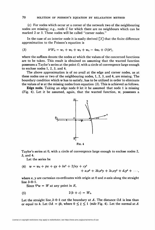
Edge node. Taking an edge node 0 let it be assumed that node 1 is missing

(Fig. 4). Let it be assumed, again, that the wanted function, w, possesses a

Taylor's series at 0, with a circle of convergence large enough to enclose nodes 2,

3, and 4.Let the series be

(4) w = Wo + px + qy + bx2 + 2fxy + cy2

+ aix3 + 3¿>ix2y + 3cixy2 + dxy3 + • • •,

where x, y are cartesian co-ordinates with origin at 0 and x-axis along the straight

line 3-0-1.Since V2«; = W at any point in R,

(5) 2ib + c) = Wo.

Let the straight line,3-0-1 cut the boundary at A. The distance OA is less than

or equal to h. Let OA = £h, where 0 < £ < 1 ivide Fig. 4). Let the normal at .4



to the boundary make an angle a with the x-axis (i.e., 3-0-1), in the anticlockwise

direction.

The given boundary condition states that

(6) idw/dv)A = kA.

Since dw/dv = k all along the boundary, it can be derived that

(7) id2w/dsdv)A = idk/ds)A,

on assuming that k possesses a derivative along the boundary at A. [d/ds denotes

the rate of change along the boundary.]

It is easy to express idw/dv)A and id2w/dsdv)A in terms of the coefficients in

the expansion (4) since along the curve,

(8) dw/dv = dw/dx cos (x, v) + dw/dy cos (y, v)

and

(9) dhv/dsdv = d2w/dxdy\cos2ix, v) — cos2(y, v)H

+ \_d*w/dy2 — d2w/dx2~\ cos (x, v) cos (y, v)

— \/p\_dw/dx cos (y, v) — dw/dy cos (x, j»)].

Here p is the radius of curvature given by ds/dip in the usual notation. The

symbols (x, v) and (y, v) indicate the angles between the x- and the v-directions,

and the y- and the v-directions, respectively.

By differentiating the series (4) successively and substituting x = £Ä, y = 0

in the results, the following approximate values are obtained at the point A.

(10) idw/dx)A = p + 2bfr + 0(Â2),

(11) idw/dy)A = q + 2f& + 0{h2),

(12) idhv/dx2)A = 2b + Oih),

(13) id2w/dxdy)A = 2f + Oih),

and

(14) id*w/dy2)A = 2c + Oih).

Combining (6), (8), (10), and (11) we obtain

[A] kA = p cos a + q sin a + 2£A(¿> cos a + / sin a) + 0(A5).

Similarly combining (7), (9), and (10) through (14) we obtain

[B] ( —) =-p^^+ q^-^ +2{f cos 2a +c - bsina cosa] + Oih).\ ds /A pA pA


72 SOLUTION OF POISSON S EQUATION BY RELAXATION METHOD

On multiplying [A] by sec a and [B] by £A tan a sec 2a and taking the

difference,

(15) kA sec a — £A tan a sec 2aidk/ds)A

= pil + %h sin a tan a sec 2a/ pA) + g (tan a — £A sin a sec 2a/pA)

+ 26£A - (c - i)£Ä tan a tan 2a + 0(F).

On substituting the co-ordinates (0, h), ( —A, 0) and (0, — A) respectively in

the series (4), the values of w2, w3, and w4 are obtained. From these it can be

deduced that

(16)

and

w2 + Wi - 2wo = 2cA2 + O (A4)

w2 - w4 = 2Aç + O (A8)

Wz - wo = - ph + bh2 + OQi3).

Fig. 5

Combining (5), (15), and (16) to eliminate the unknown coefficients, we obtain

an elegant result,

(17) Woh2 (l + 2* j-^ ) - UkJi + m2 + 2 ( | )a |A2m j-

/ 1 + m2 A mVl + m2 \= w2[\ -m + 2S-- +f-—- )

\ 1 — m2 pa 1 — m /

+ w2

0 A m2\l -(- m2+ 2wt\l+S-

PA 1 - m2 )

/ 1 + m2 h wVl + w2\+ W4(l+m + 2£--;-*- )

\ 1 — m2 pA l + m /

iw Ji+(i±^ + (Lv^l±^) + 0V).\ 1 — m2 _ pa 1 — »î2 /

where jm = tan a.



The first member of this equation can be calculated at every one of the edge

nodes, as soon as a suitable square net is fitted to the region of integration, since

this expression depends only on the given functions W and k, and the character-

istics of the boundary curve. Similarly all the coefficients of the w on the right

hand side can be determined at the outset.

Corner node. The method of obtaining a residual formula at a corner node

involves a few geometrical constructions, which are indicated in Fig. 5 for the

case in which nodes 1 and 2 are missing. Taking our stand for a moment at 0' in

Fig. 5, we can derive as we have done above, that

(18) tFo-^Tl + 2? 1 - V2AAaVi + m2 + (~) th2m\2 L 1 — m2 J \ ds/A

= wz ( 1 -

1 +m2

wr

*(+ 2Wl I 1 + £

1 + m2 h wVl + m2

1 - m2 V2pa 1 - »»

A m2<\ +m2\

V2pa ! - m

( 1 + m2 h f»Vl + m2\+ Wi[l + m + 2£--:-í-7=-7—-)

\ 1 — m2 V2pA 1 + » /

/ 1+w2 A Vl + m2 \-4w0.(l +i--2 + tH^-m-i-7) + Oih3).

\ \ — m2 V2PA I - m2 /

The positions of 0' and A are to be noted carefully. Again

0'-3 = 0'-7 = 0'-4 = A/V2.

Hence (18) is obtained from (17) by merely replacing.A by A/V2 and giving suffixes

to w in accordance with Fig. 5. It is to be noted that £ > 1 here.

Because of Poisson's equation,

A2(19) — Wo- = wo + Wa + Wi + Wi — 4w0' + 0(A4).

On eliminating Wo' between (18) and (19) we obtain

(20) Wo-^Ç- <2hkA Vl +m2 + ( js Ja %h2m ^1 + w2

m2

1 + m2 fA wVl + jw2'Wz \ — m + ? ;-r +

1 - m2 V2pa 1(-

/ y 1 + m2 , £Ä 9 Vl +m2\+ wAl - £- + -v=— -m2 —- )

\ 1 — m2 V2pa 1 — m2 /

(+ Wi \ m + £

1 + m2 ¿A mVl + m2 '

1 - w2 V2pa 1 nv

/ 1 + w2 £A w2Vl + m2 \- too ( 1 + £ :-; + -rp-:-— ) + Oih3).

\ 1 — m2 V2pA 1 — w2 /



v"3,

S


SOLUTION OF POISSON'S EQUATION BY RELAXATION METHOD

oo po

O OPO po

O ÖI I

in 10 »o oo,-h r- vo voes CS ^H es

oI

J a i

I I I

s JOO o

.1 sV£> o >o

m' O « U)

3CS VO

CM lO es POrt ■* OV

S s svo

(N

+ + + + + + + +

I+ + + + I + I +

o ») 6es O ■*.-< PO 00

•i ^h ^h es

S S Svo es oovo es vo

Tí

es ~h ~-

1e

I

^l^à

(N h lO\0 <N ^hlO O 00

g es

O 00

Ö OI I

po « e*ov ■■* -H<* <m Q^H O v-l

O O O

VO C3V riPO PO ~H•* PO •*t^ VO IO

Ö Ö Ö

■* oO lO00 vo

Ö ©

te;

I3

Ifl N Ul ^ CAt* 00 VO — O-to vo Ov -^ eses es es po -*fO Ö es O ÖI I I I I

oo esvo OOtO 00

Ö ÖI I

«o»o

1o «po on

ö ö

VO voW O

Ö o

•HtoÖ

H

n

'S

■Eo¿

U

•^ O O Ov r-»— ï^ ~H LO LO

«, po es Ov ro esO — es VO 00

O « O O Ö

S gpo o esoo *- vovo es voOv Ov 00

es o es

es «

"O vppo es

es es

vo

oo rc vo es-* .^ rH es

& vV V V V

>. bfi bo ojo bd u¿O -a ~a -o -a o^ W W W w u

T3 Ow u

■3U

o <# <; ^ ^ ^ te; te; te;



The important points about this formula are :

(i) The value of W to be taken is the value at 0' and not that at 0.

(ii) A change in the assumed value of w at node 7 will affect the residual at 0

but not vice versa.

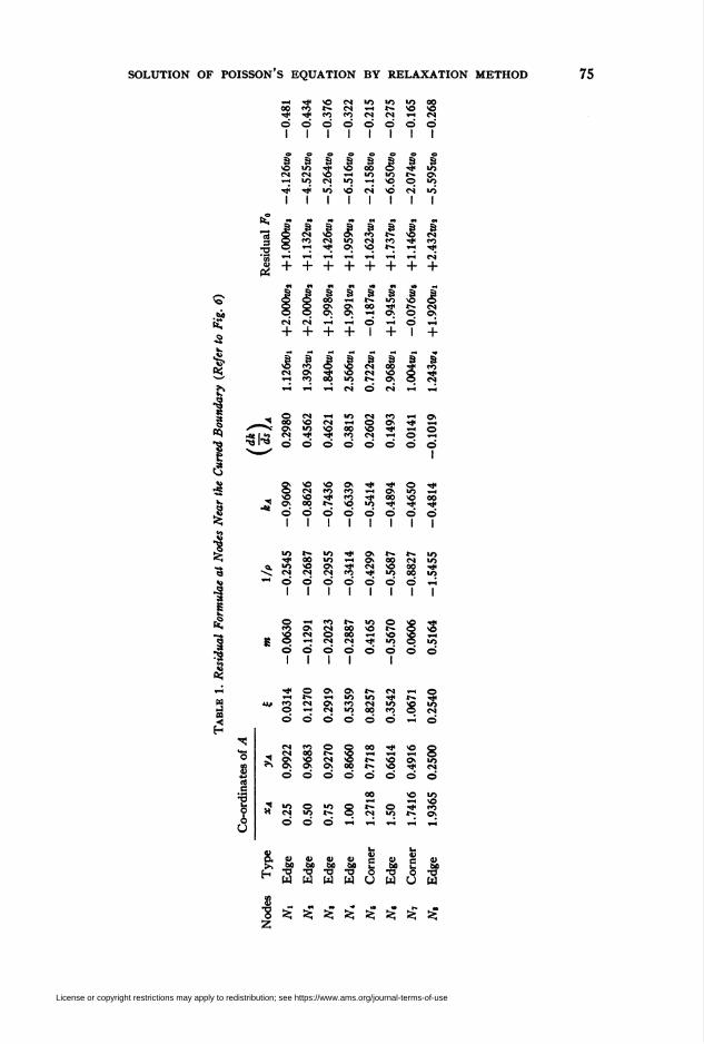
Illustrative Example. The above formulae were applied to calculate the values

of w — log r >■ i log (x2 + y2) within the region BCDEFB shown in Fig. 6,

assuming dw/dv to be given all along the boundary. It is well known that log r

satisfies Laplace's equation in any region of the plane, provided the origin is

outside the region. Hence W = 0 in equation (1).

The curved boundary FB is part of the ellipse

x2/4 + y2 = 1.

BC and EF lie along the x- and y-axes respectively, while CD lies along the line

x = 3, and DE along the line y = 2.

The network adopted is rather coarse with A = 0.25 only. There are eight

nodes besides F and B, which lie adjacent to the elliptic boundary. They are

numbered in order in Fig. 6. Of these nodes, N6 and iV7 are corner nodes and the

rest, edge nodes. Hence equations (17) and (20) are directly applied to these

nodes. Table 1 summarizes all the data required at these nodes for calculating

the coefficients in equations (17) or (20), and also gives the corresponding residual

formulae.Table 2

Nodes Residual

F Fo = wx + w2 - 0.250B Fo = wx + w2 - 0.125C Fo = w2 + wz + 0.083D Fo = wz + Wi + 0.096E F0 = Wi + wx + 0.125

At nodes F and B the missing nodes are eliminated from equation (3) by

making use of the values dw/dx and dw/dy which are both known there. The same

is the case at nodes C, D, and E. The residual formulae for these nodes are given

in Table 2.

At all intermediate nodes on BC, CD, DE, and EF, one of the surrounding

nodes is missing and this is eliminated from (3) as either dw/dy or dw/dx is known

at these nodes. (Alternatively the same result can be obtained from equation

(17) by setting £ = m = 1/p = 0.) The residual formula at a node on BC, for

example, will take the form

Fo = wx + 2w2 + Wz — iwo + 2hko = OQi3).

It may be noted that the problem as set up so far is indeterminate in the sense

that any constant value can be added to a solution that satisfies the conditions

of the problem. For

if V2w = W inside a region R,

and dw/dv = k on the boundary of R,



it is clear that

v^(w + c) = W inside R,

and

d/dviw + c) = k on the boundary,

where c has the same value at all points. This property is reproduced in the set

of residual formulae derived above. Every one of these formulae has the feature

iif J.U zzf un ¿o" ,to iho ifa. as no_18 »í 9b

Fig. 6A. The Start : w assumed zero at all nodes. The non-zero residualsmultiplied by 103 are shown here

68*. 6l7-* -7/1, -ISS* gola. g.55. 1'3, 974, IQ3¿/ '°?8 J. "60. iao , ia71 h

Fig. 7. The End: Values of w multiplied by 103 are shown. Final residuals are given



that the sum of the coefficients of the unknown w is zero. Hence if a set of values

of w give rise to a certain set of residuals, then the set of values (w + c) where c

is the same for all nodes, will also give rise to the same set of residuals. It is,

therefore, necessary to give the value of w at some point in order to make the

solution unique. We make use of the fact that log r = 0 at F for this purpose.

Starting with the initial guess w = 0 at all nodes, the solution exhibited in

Fig. 7 was obtained by the method of relaxation. The initial residuals are shown

in Fig. 6A. During the process of relaxation of the residuals, negative values were

obtained for w at nodes like F, NL, etc. ivide, Fig. 6). When all the residuals had

become negligible, a suitable value was added at all the nodes so as to bring the

value of w at F to zero.

The values of log r for select values of r as taken from Fig. 7 are compared in

Table 3 with the true values taken from a standard table of Mathematical

Table 3

Log r Log r

by re- true by re- truer laxation value Node r laxation value

1.00 0.000 0.000 Nx 1.0308 0.030 0.0301.25 0.221 0.223 N2 1.1180 0.110 0.111

1.50 0.402 0.405 Ns 1.2500 0.221 0.2231.75 0.556 0.560 N* 1.4142 0.345 0.3472.00 0.689 0.693 N6 1.4577 0.373 0.3772.25 0.806 0.811 7Y6 1.6771 0.513 0.5172.50 0.911 0.916 Ni 1.8200 0.594 0.5992.75 1.006 1.012 Ng 2.0156 0.696 0.7013.00 1.093 1.099 D V13.0000 1.279 1.282

Functions, see F. Castle [4]. The agreement is remarkable in spite of the network

being coarse.

The author is indebted to D. N. de G. Allen of the Imperial College of Science,

London, for the interest shown by him in the publication of this article, when he

visited the University of Roorkee, India.

Messrs. C. M. Ganesan and G. Natarajan have been of valuable help to the

author in the preparation of the typescript.

R. V. VlSWANATHAN

Central Water and Power Commission

Government of India

New Delhi, India

1. R. V. Southwell, Relaxation Methods in Theoretical Physics, Oxford, at the ClarendonPress, 1946.

2. L. Fox, "Numerical solution of elliptic differential equations when the boundary conditionsinvolve a derivative," Roy. Soc., Phil. Trans., London, v. 242, 1950, p. 345-378.

3. D. N. de G. Allen, Relaxation Methods, McGraw Hill Book Co., Inc., New York, 1954.4. F. Castle, Five-Figure Logarithmic and Other Tables, Macmillan and Co., London, 1910.


solution of poisson's equation by relaxation method—normal ......solution of poisson's...

Documents